Inferences on Mass Composition and Tests of Hadronic Interactions from 0.3 to 100 EeV using the water-Cherenkov Detectors of the Pierre Auger Observatory

Abstract

We present a new method for probing the hadronic interaction models at ultra-high energy and extracting details about mass composition. This is done using the time profiles of the signals recorded with the water-Cherenkov detectors of the Pierre Auger Observatory. The profiles arise from a mix of the muon and electromagnetic components of air-showers. Using the risetimes of the recorded signals we define a new parameter, which we use to compare our observations with predictions from simulations. We find, firstly, inconsistencies between our data and predictions over a greater energy range and with substantially more events than in previous studies. Secondly, by calibrating the new parameter with fluorescence measurements from observations made at the Auger Observatory, we can infer the depth of shower maximum X_max for a sample of over 81,000 events extending from 0.3 EeV to over 100 EeV. Above 30 EeV, the sample is nearly fourteen times larger than currently available from fluorescence measurements and extending the covered energy range by half a decade. The energy dependence of $\langle$X_max$\rangle$ is compared to simulations and interpreted in terms of the mean of the logarithmic mass. We find good agreement with previous work and extend the measurement of the mean depth of shower maximum to greater energies than before, reducing significantly the statistical uncertainty associated with the inferences about mass composition.

I Introduction

Our understanding of the properties of the highest-energy cosmic rays has grown enormously over the last 12 years with the advent of data from the Pierre Auger Observatory and the Telescope Array. These devices have been used to study the energy spectrum, the mass composition and the distribution of arrival directions of cosmic rays from 0.3 EeV to energies beyond 10 EeV. While the features of the energy spectrum and of the arrival directions have been well-characterised up to $\sim$100 EeV, the situation with regard to the mass spectrum is less satisfactory because of the reliance on models of the hadronic physics. This state of affairs arises for two reasons. Firstly, the method that provides the best resolution, and therefore is the most potent for measuring a mass-sensitive feature of extensive air-showers, is the fluorescence technique. It has been exploited on an event-by-event basis to determine the depth of shower maximum, i.e. the depth in the atmosphere at which the energy deposition in the shower is greatest, but, as observations are restricted to clear moonless-nights, the number of events is limited. For example, in the Auger data so far reported (up to 31 December 2012) there are 227 events above 16 EeV r1 . For the same energy range, the event number from the Telescope Array is smaller, 25 r2 . Secondly, to interpret the data sets from the water-Cherenkov detectors and the fluorescence telescopes, one must use the predictions of features of hadronic interactions, such as the cross-sections for proton and pion interactions, the multiplicity and the inelasticity, at centre-of-mass energies up to $\sim$300 TeV, well-beyond what is accessible at the LHC r3 .

To overcome the limitations imposed by the relatively small number of events accumulated with the fluorescence technique at the highest energies, use can be made of data recorded with the water-Cherenkov detectors of the Observatory which are operational nearly 100% of the time and thus yield substantially more events at a given energy. In this paper, we describe a new method for extracting information about the development of air showers from the time profiles of the signals from the water-Cherenkov detectors.

Our method allows a comparison of the data with predictions from models of parameters inferred directly from these detectors in which a signal from a mix of the muon and electromagnetic components of air-showers is available. This approach follows the line opened in four recent studies. From comparisons of Auger observations with hadronic models it is argued that the latter are inadequate to describe the various measurements r4 ; r5 ; r6 ; r7 . As in the earlier work, we find that there are inconsistencies between the models and the data: this is established over a greater energy range and with more events than before.

The method also enables us to infer the depth of shower maximum (a dominantly electromagnetic measurement) by calibrating the new parameter with measurements from the fluorescence telescopes. We have determined X_max for about three times more events than available from these telescopes alone over the range from $\sim$0.3 EeV to beyond 70 EeV: specifically for the two surface detector configurations, the 750 and 1500 m arrays r8 , there are 27553 and 54022 events recorded respectively for which estimates of X_max have been possible. Of those, 49 events are in the range beyond 70 EeV, and 1586 above 20 EeV.

The structure of the paper is as follows. In section II features of the Pierre Auger Observatory are briefly outlined. The measurement of the risetime of signals from the water-Cherenkov detectors is described in section III and the new parameter for studying the depth of shower maximum is introduced in section IV. A comparison of the new parameter with predictions from hadronic models is discussed in section V. Section VI presents the results on the measurement of average X_max from 0.3 EeV to beyond 70 EeV. A summary of the conclusions is given in section VII.

II The Pierre Auger Observatory

The Pierre Auger Observatory is located near the city of Malargüe in the Province of Mendoza, Argentina. It is a hybrid system, being a combination of a large array of surface detectors and a set of fluorescence detectors, used to study cosmic rays with energies above 0.1 EeV. Full details of the instrumentation and the methods used for event reconstruction are given in r8 .

The work presented here is based on data gathered from 1 Jan 2004 to 31 Dec 2014 from the surface-detector array (SD), which covers an area of over 3000 km². The array contains 1660 water-Cherenkov detectors, 1600 of which are deployed on a hexagonal grid with 1500 m spacing with the remainder on a lattice of 750 m covering 23.5 km². We refer to these configurations as the 1500 m and 750 m arrays. The water-Cherenkov detectors are used to sample the electromagnetic and muonic components of extensive air-showers. Each detector contains 12 tonnes of ultra-pure water in a cylindrical container, lined with Tyvec, 1.2 m deep and of 10 m² area. The water is viewed by three 9”-photomultiplier tubes (PMTs). Signals from the anode and an amplified signal from the last dynode of each PMT are digitised using 40 MHz 10-bit Flash Analog to Digital Converters (FADCs): these are called the ‘high-gain’ and ‘low-gain’ channels in what follows. The responses of the detectors are calibrated in units of the signal produced by a muon traversing the water vertically at the center of the station: this unit is termed the “Vertical Equivalent Muon” or VEM r9 . Air showers are identified using a 3-fold coincidence, satisfied when a triangle of neighbouring stations is triggered r10 . Using the six FADCs, 768 samples (over 19.2 $\mu$s) are recorded at each triggered station. For the present analysis events are used that are confined within the array so that an accurate reconstruction is ensured. This requires that all six stations of the hexagon surrounding the detector with the highest signal are operational and is known as the 6T5 condition. The arrival directions are found from the relative arrival times of the shower front at the triggered stations. The angular resolution is 0.8^o for energies above 3 EeV for the 1500 m array and 1^o for the 750 m-configuration r8 .

The estimator of the primary energy is the signal reconstructed at 1000 m (1500 m array) or 450 m (750 m array) from the shower core, denoted by S(1000) and S(450) respectively. These estimators are determined, together with the core position, through a fit of the recorded signals (converted to units of VEM after integration of the FADC traces) to a lateral distribution function that describes the average rate of fall-off of the signals as a function of the distance from the shower core. For S(1000) > 20 VEM (corresponding to an energy of $\sim$3 EeV) showers are recorded with full efficiency over the whole area of the array. For the 750 m array, the corresponding value of S(450) for full efficiency is $\sim$60 VEM ($\sim$0.5 EeV). The accuracy of the core location in lateral distance is $\sim$50 m (35 m) for the two configurations. The uncertainty of S(1000), which is insensitive to the lateral distribution function r11 , is 12% (3%) at 3 EeV (10 EeV) and for S(450) the corresponding figure is 30% at 0.5 EeV.

The conversions from S(450) and S(1000) to energy are derived using subsets of showers that trigger the fluorescence detector and the surface array independently (‘hybrid events’) using well-established methods r12 . The statistical uncertainty in the energy determination is about 16% (12%) for the two reference energies of the 1500 m array and 15% at 0.5 EeV for the 750 m array. The absolute energy scale, determined using the fluorescence detector, has a systematic uncertainty of 14% r13 .

Twenty-four telescopes (each with a field of view of 30^o$\times$30^o) form the Fluorescence Detector (FD). They are distributed in sets of six at four observation sites. The FD overlooks the SD array and collects the fluorescence light produced as the shower develops in the atmosphere. Its duty cycle amounts to $\sim$15% since it operates exclusively on clear moonless nights. The 750 m array is overlooked from one observation site by three high-elevation telescopes (HEAT) with a field of view covering elevations from 30^o to 60^o, thus allowing the study of lower energy showers. Those low energy showers are detected closer to the detector; therefore we need a higher elevation field of view to contain also this kind of events.

III The Risetime and its Measurement

III.1 Overview of the risetime concept

In the study described below, we use the risetime of the signals from the water-Cherenkov detectors to extract information about the development of showers. A single parameter, namely the time for the signal to increase from 10% to 50% of the final magnitude of the integrated signal, t_1/2, is used to characterize the signal at each station. This parameter was used for the first demonstration of the existence of ‘between-shower’ fluctuations in an early attempt to get information about the mass of the cosmic rays at $\sim$1 EeV r14 . That work was carried out using data from the Haverah Park array in England where the water-Cherenkov detectors were of 1.2 m deep (identical to those of the Auger Observatory) and of area 34 m².

The choice of this parameter is based on the experimental work by Linsley and Scarsi r15 . They showed that at distances of more than about 100 m from the shower core, the early part of the shower signal is dominated by muons. Direct measurements of muons using magnetic spectrographs established that the mean momentum of muons beyond 100 m was more than 1 GeV: this leads to the conclusion that the geometrical effects dominate the temporal spread of the muons at a detector. This is illustrated in Fig. 1 for a shower arriving in the vertical direction where it can be seen that the muons arriving from lower down in the shower arrive later at a detector than those that arise from higher up. Furthermore it is evident that at larger distances from the shower axis, the muons will be more dispersed in time than at smaller distances, leading to the dependence of the risetime on distance found experimentally (Fig. 2). Because the muons are relatively energetic, the effects of velocity difference, of deflections in the geomagnetic field and of Coulomb scattering is small although these factors were taken into account even in the earliest Monte Carlo studies of the phenomenon r16 . By contrast the electrons and photons of an air shower have mean energies of about 10 MeV so that the arrival of the electromagnetic component of the shower is delayed with respect to the muons because of the multiple scattering of the electrons. The delay of the electromagnetic component with respect to the muons also increases with distance.

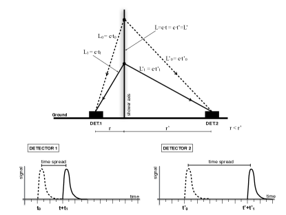
Figure 1: Qualitative sketch of how geometrical effects affect the temporal spread of the muons at a detector.

The risetime is found experimentally to be a function of distance, zenith angle and energy (Fig. 2). At 1000 m from the shower axis, for a vertical event of 10 EeV, t_1/2 $\sim$380 ns. This value increases slowly with energy and decreases with zenith angle. At large angles and/or small distances t_1/2 can be comparable to the 25 ns resolution of the FADCs and this fact restricts the data that are used below. The fastest risetime, measured in very inclined showers or with single muons, is 40 ns and is an indication of the limitations set by the measurement technique and hence guides our selection of distance and angular ranges.

Because of the size of the Auger Observatory and the large separation of the detectors, it is necessary to take account of the fact that a detector that is struck early in the passage of the shower across the array will have a slower risetime than one that is struck later, even if the two detectors are at the same axial distance from the shower core. This asymmetry arises from a complex combination of attenuation of the electromagnetic component as the shower develops and because of the different part of the angular distribution of muons (more strictly of the parent pions) that is sampled at different positions across the array. The attenuation of the electromagnetic component of a shower across an array was first discussed by Greisen r17 . A detailed description of the asymmetry that is observed, and of its power for testing hadronic interaction models, has been given recently r6 . For the present study, the asymmetry is taken into account by referencing each risetime to that which would be recorded at a hypothetical detector situated at 90^o with respect to the direction of the shower axis projected onto the ground, and at the same axial distance from the shower core, as the station at which a measurement is made. The amplitude of the asymmetry is a function of zenith angle, axial distance and energy: at 40^o, 750 m and 10 EeV it is $\sim$15%.

The magnitudes of the risetimes that are measured in a particular shower depend upon the development of the shower. As the energy increases, the mean position of the point of maximum development of the shower moves deeper into the atmosphere and thus the risetimes will, on average, be slower than for a lower energy event. Because muons dominate the shower to an increasing extent at large zenith angles, because the electromagnetic component suffers increased attenuation, the risetimes are expected to be faster at a detector that is at the same distance from the axis of the shower but in the vertical direction. The magnitude of the energy, distance and zenith angle effects that can be inferred qualitatively from Fig. 1 are evident in the data shown in Fig. 2.

From these considerations, it follows that studying the risetimes of showers provides a method of measuring the shower development and thus of deducing the mass composition. Details of the study are presented below where the risetime properties are also compared with predictions from Monte Carlo calculations using different hadronic models.

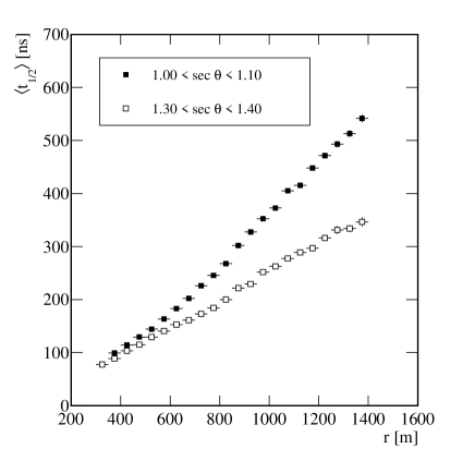
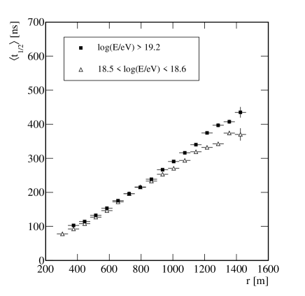
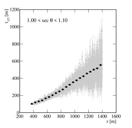
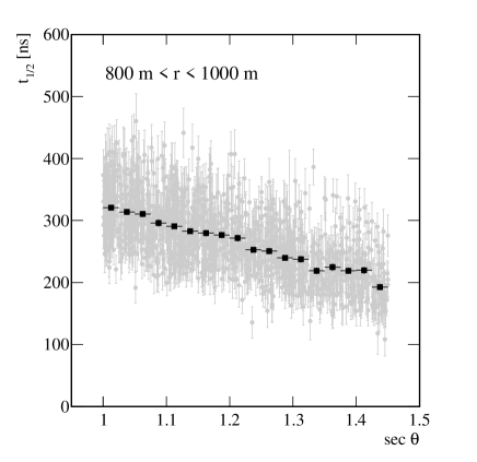
Figure 2: (Top left) The risetime as a function of distance to the shower core for two different intervals of sec $\theta$ in the energy range 19.0 < log (E/eV) < 19.2. (Top right) The risetime as a function of distance for two different energy bands in the angular range 1.20 < sec $\theta$ < 1.30. (Bottom left) Illustration of the spread in the risetimes as a function of distance for events in the energy range 19.1 < log (E/eV) < 19.2. (Bottom right) Illustration of the variation of risetime with zenith angle for events in the energy range 19.1 < log (E/eV) < 19.2. All plots are based on experimental data

III.2 Determination of the accuracy of measurements of t_1/2

The uncertainty in a measurement of t_1/2 is found empirically from the data and will be described in some detail as it plays an essential role in the determination of the new parameter, introduced in section IV, used to characterize shower development. The uncertainty can be obtained by using sets of detectors placed 11 m apart (known as ‘twins’) and also by using detectors that lie at similar distances from the shower core (‘pairs’). Measurements made using twins and pairs cover different distance ranges. With twins we can parameterize the uncertainty with a sufficient number of events only between 300 m and 1200 m from the shower core. With pairs we can cover distances from 600 m to 1800 m. It is then natural to combine both sets of measurements to avoid as much as possible relying on extrapolations when estimating the uncertainty in the measurement of t_1/2.

The twin detectors give two independent measurements of the risetime at what is effectively a single point in the shower plane. Differences in the values of t_1/2 at the twins arise from the limitations set by the sampling of the shower front by a detector of finite size (10 m²) and from the measurement uncertainties intrinsic to the FADC system. For the more-numerous pairs there are the additional complications that arise from the asymmetry effect and from the difference in distance of the pairs from the shower core.

III.2.1 Assessment of measurement uncertainty using twin detectors

In the surface-detector array there are 14 sets of twins and seven sets of triplets (three detectors on a triangular grid each separated by 11 m): the triplets are also referred to as ‘twins’. We parameterize the uncertainty by splitting the data in different bins of distance to the core, zenith angle and detector signal. This implies that a precise parameterization of the uncertainty demands a large amount of data. To cope with this requirement we must combine all twin measurements that belong to events reconstructed at either of the arrays. A total of $\sim$83 000 twin measurements are available from the two arrays for zenith angles below 60^o and above energies of 0.3 EeV and 1 EeV for events that trigger the two arrays. The cuts on energy and zenith angle are very loose to enhance the number of events available for analysis. Likewise the criteria applied at detector level and detailed in Table 1 are mild to keep the selection efficiency as high as possible. We discard detectors that recorded a small number of particles or located far from the core to avoid biases in the signal measurement. For very large signals, the risetime measurements approach the instrumental resolution and therefore are discarded. The cut on |S_i – S_mean| in Table 1 is made to deal with cases where one signal is typically around 5 VEM and the other, possibly because of an upward fluctuation, is relatively large. Such twins are rejected.

The average uncertainty in a risetime measurement, $\sigma$_1/2, is given by

$$\sigma_{1/2}=\frac{\sqrt{\pi}}{2}\left\langle\left|t_{1/2}^{1}-t_{1/2}^{2}\right|\right\rangle$$ (1)

where the superscripts define each member of the twin. As twin detectors are only 11 m apart no correction is necessary for the azimuthal asymmetry.

Table 1: Selection of twin detectors used to assess the risetime uncertainty.

	750 m array		1500 m array
Cuts	Number of twins	Efficiency	Number of twins	Efficiency
Pre-twin selection	41 100	1.00	41 934	1.00
5 < S/VEM < 800	34 461	0.84	35 704	0.85
r < 2000 m	34 459	0.83	35 620	0.84
|Si-Smean|< 0.25 Smean	28 466	0.69	29 832	0.71

The data have been divided into seven sec $\theta$ intervals (of width 0.1) and six distance ranges (see Fig. 3 left). The mean values of $\sigma$_1/2 as a function of signal size, S, are fitted with the function

$$\sigma_{1/2}\,=\sqrt{\left(\frac{J(r,\theta)}{\sqrt{S}}\right)^{2}+\left(\sqrt{2}\frac{25\,\text{ns}}{\sqrt{12}}\right)^{2}}$$ (2)

The first term in this function represents the differences seen between the two detectors while the second term arises from the digitisation of the signal in time intervals of 25 ns.

J is found from a linear function, J(r,$\theta$) = p_o($\theta$) + p₁($\theta$) r, and the fitted values of p_o and p₁ as functions of sec $\theta$ are

$$\begin{array}[]{l}p_{0}(\theta)=(-340\pm 30)+(186\pm 20)\,\sec\theta\\ p_{1}(\theta)=(0.94\pm 0.03)+(-0.44\pm 0.01)\,\sec\theta\end{array}$$ (3)

where p₀ units are (ns VEM^1/2) and p₁ units are (ns VEM^1/2 m^-1).

III.2.2 Assessment of measurement uncertainty using pairs of detectors

For the purposes of this study, a pair of detectors is defined as any two detectors in the same shower where the difference in distance from the shower core, (|r₂ – r₁|) is less than 100 m, irrespective of azimuth angle. After applying the cuts previously discussed, there are $\sim$50% more pair measurements than there are measurements from twins. This sample is large enough to allow us to limit this study to pairs of detectors from the 1500 m array only. However, corrections have to be made for the asymmetry and, because of the array spacing, there are no data below 600 m. Additionally a correction must be made because the risetimes are at different axial distances: for a 100 m separation this difference is $\sim$30 ns, assuming a linear dependence of risetime with distance (see Fig. 2). Before applying this correction the mean time difference for pairs was (14.750 $\pm$ 0.002) ns: after correction the average difference was (0.140 $\pm$ 0.002) ns.

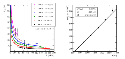
Figure 3: (Left) Uncertainty obtained with pair detectors as a function of the station signal for vertical events (1.00< sec $\theta$ <1.10). Each line is the result of the fits performed for different distance ranges. Each point represents the average measurements of at least 10 pair detectors. (Right) The parameter J(r, $\theta$) as a function of the distance to the core for the same zenith angle range.

From a similar analysis to that described for the twin detectors, the fits for p₀ and p₁ have the parameterisations

$$\begin{array}[]{l}p_{0}(\theta)=(-447\pm 30)+(224\pm 20)\,\sec\theta\\ p_{1}(\theta)=(1.12\pm 0.03)+(-0.51\pm 0.02)\,\sec\theta.\end{array}$$ (4)

The variation of J with distance is also shown in Fig. 3.

The differences in the values of p₀ and p₁ from the two analyses arise because they cover different distance ranges and different energy ranges. To optimize the determination of $\sigma$_1/2 for the risetimes measured at each station, we adopt the following parameterisations for p₀ and p₁ for different core ranges

$$\begin{array}[]{l}p_{0}(\theta)=\begin{cases}(-340\pm 30)+(186\pm 20)\,\sec\theta,\,\,r\leq\,650\,\text{m}\\ (-447\pm 30)+(224\pm 20)\,\sec\theta,\,\,r>\,650\,\text{m}\\ \end{cases}\\ p_{1}(\theta)=\begin{cases}(0.94\pm 0.03)+(-0.44\pm 0.01)\,\sec\theta,\,\,r\leq\,650\,\text{m}\\ (1.12\pm 0.03)+(-0.51\pm 0.02)\,\sec\theta,\,\,r>\,650\,\text{m}\\ \end{cases}\end{array}$$ (5)

We have set the break point at 650 m because at this distance the uncertainties given by the two parameterizations agree within their statistical uncertainties (2-3 ns).

IV The new parameter $\Delta_{s}$ and its determination for individual air-showers

IV.1 Introduction to the Delta method

When a large number of risetimes is recorded in an event, it is possible to characterize that event by a single time just as the size of an event is designated by S(1000), the signal size at 1000 m from the shower axis. This approach is only practical at high energies, as several measurements are needed to estimate the risetime at 1000 m by extrapolation r18 . Here, to obtain a large sample of data over a wide range of energies, an alternative method of using risetime measurements is introduced. We have determined for the two arrays independent relationships that describe the risetimes as a function of distance in a narrow range of energy (see section IV.3). We call these functions ‘benchmarks’, and risetimes at particular stations, after correction for the asymmetry effect, are compared with the relevant times from the benchmark, $t_{\text{1/2}}^{\text{bench}}$, in units of the accuracy with which they are determined. The approach is illustrated in Fig. 4: the benchmarks are, of course, zenith-angle dependent (see Fig. 2). We use the term ‘Delta method’ to refer to this approach in what follows.

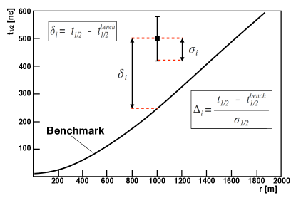
Figure 4: Schematic diagram to illustrate the Delta method.

Thus for each measurement of t_1/2 at a single detector, i, an estimate of $\Delta_{i}=\left(t_{\text{1/2}}-t_{\text{1/2}}^{\text{bench}}\right)/\sigma_{\text{1/2}}$ is made. Each shower is then characterised by $\Delta_{s}$, the average of these estimates for the N selected stations.

$$\Delta_{s}=\frac{1}{N}\sum\limits_{stations}\Delta_{i}$$ (6)

IV.2 Data selection

The data from the water-Cherenkov arrays were collected between 1 Jan 2004 (2008 for the 750 m spacing) and 31 Dec 2014. The first selection, of 6T5 events, has already been discussed. Other selections for the two arrays are shown in Table 2.

Table 2: Quality cuts applied to the events of the 750 m and the 1500 m arrays. $\epsilon$ stands for the overall efficiency. The explanation for the different cuts can be found in the text.

750 m array			1500 m array
Quality cuts	Events	$\epsilon$ (%)	Quality cuts	Events	$\epsilon$ (%   )
17.5 < log (E/eV) < 18.5	159 795	100.0	log (E/eV) > 18.5	217 469	100.0
sec $\theta$ < 1.30	72 907	45.6	sec $\theta$ < 1.45	97 981	45.0
6T5 trigger	29 848	18.7	6T5 trigger	67 764	31.0
Reject bad periods	28 773	18.0	Reject bad periods	63 856	29.0
$\geq$ 3 selected stations	27 553	17.2	$\geq$ 3 selected stations	54 022	24.8

The lower energy cuts are made to select events that trigger the arrays with 100% efficiency. The upper energy cut in the 750 m array is made to set aside events in overlapping energy regions that will be used later to cross-check the robustness of the method. As previously discussed, at large angles t_1/2 can be comparable to the 25 ns resolution of the FADCs and this fact restricts the usable angular range. The cut in zenith angle is lower for the 750 m array than for the 1500 m array because the stations tend to be closer to the core and the limitations set by the sampling speed of the FADCs become more important at larger angles and small distances. We rejected data taking periods where the performance of the array of surface detectors was not optimal. At least three selected stations are required for an event to be included in the data samples.

The stations used within each event must fulfil the following criteria. The stations cannot be saturated in the low-gain channel since risetimes cannot be obtained from such signals. The signals recorded by the stations must be bigger than 3 VEM and 5 VEM for the 750 m and the 1500 m arrays respectively. Those cuts guarantee that no bias towards primaries of a particular type is introduced: the difference in selection efficiency for protons and iron is less than 5% for all energy bins. The selected stations must lie within a given distance range from the position of the reconstructed core of the shower. The lower range of distance, 300 m, is selected to avoid the problems set by the inability of the recording system to record fast pulses (see section III.1), while the upper ranges (800 m (1400 m) for the 750 m (1500 m) array) are chosen to span what is consistent with unbiased selection. For the highest energies this has been extended to 2000 m as the signal sizes in such events are sufficiently large to give accurate measurements. For the 750 and 1500 m arrays the overall selection efficiencies at station level are 52% and 56% respectively. This translates into 113,661 and 210,709 detectors for the 750 m and the 1500 m arrays respectively.

Using simulations, we have searched for biases that might be introduced into inferences about mass composition as a result of these cuts. The difference between the overall selection efficiencies for protons and Fe-nuclei are smaller than 2%. The upper limit on the energy cut in the 750 m data eliminates only 2% of the events. This cut, and the lower energy limit for the 1500 m array, are relaxed later to study the overlap region in detail.

For the 750 and 1500 m arrays, the mean numbers of selected stations per event satisfying the selection criteria defined in Table 2 are 4.0 and 3.6 respectively. In the analysis discussed below, selected events are required to have 3 or more values of $\Delta_{i}$, but, for an arrival direction study, in which it is desirable to separate light from heavy primaries, one could envisage using two stations, or even one, to infer the state of development of the shower, albeit with more limited accuracy.

IV.3 Determination of the benchmarks for the 750 and 1500 m arrays

The determination of the benchmarks, which define the average behaviour of the risetimes as a function of distance and zenith angle, is fundamental to the success of the technique. Essentially the same procedures have been adopted for both arrays. For each detector two time traces are recorded on high-gain and low-gain channels. The risetime of a detector is computed according to the following procedure: in the case where no saturation occurs, the risetime is obtained from the trace corresponding to the high-gain channel. If this channel is saturated, we use the trace from the low-gain channel to compute the risetime. If the low-gain signal is saturated as well, which can occur for stations close to the core in high-energy events, that station is not selected for this analysis. Further details of the recording procedures are given in r8 .

In computing the benchmarks, account must be taken of the fact that the risetimes measured for a station in the two channels are not identical, as illustrated in Fig. 5. During the digitization process, a threshold is imposed that removes very small signals. The net effect of this threshold affects the low-gain traces much more, since their signals are smaller due to the lower signal-to-noise ratio when compared to the one associated to high-gain traces. The influence of tails in the determination of the integrated signal is therefore reduced for low-gain signals and as a consequence the risetime measurement is affected. This instrumental effect makes it necessary to obtain benchmarks for the high-gain and the low-gain traces independently.

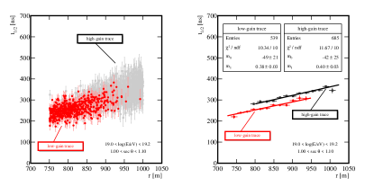
Figure 5: (Left) Risetimes as a function of core distance for events with and without saturation in the high-gain channel. We have selected events with energies 19.0 < log (E/eV) <19.2 and zenith angles 1.00 < sec $\theta$ <1.10. (Right) Same as left plot but this time we show average values to make more evident the difference between measurements when the saturation of the high-gain channel is present.

As shown in Table 2 the energy ranges covered by the two arrays are 17.5 < log (E/eV) < 18.5 (750 m spacing) and log (E/eV) >18.5 (1500 m spacing). The energy bins chosen for the benchmarks of the 750 and 1500 m arrays are 17.7 < log (E/eV) < 17.8 and 19.1 < log (E/eV) < 19.2 respectively. The choices for the benchmarks are most effective in dealing with the high-gain/low-gain problem just discussed. They guarantee that we reject a reduced number of detectors where the low and the high-gain channels are simultaneously saturated and therefore allow a definition of the benchmark over a broad distance range. In addition, this implies that the distance intervals used to fit the behaviour of the risetimes computed either with the low or the high-gain traces are sufficiently long to avoid compromising the quality of the fit.

A fit is first made to the data from the low-gain channels using the relation

$$t_{\text{1/2}}^{\text{low-gain trace}}=40\,\text{ns}+\sqrt{A(\theta)^{2}+B(\theta)r^{2}}-A(\theta)$$ (7)

where A and B are free parameters. The reason for adopting 40 ns as a limit was explained in section III.1. Other functions were tested: this one gave consistently lower values of reduced $\chi^{2}$ over the range of angles and energies used for the two arrays.

Having used low-gain traces to evaluate A and B, the signals from high-gain traces are now fitted with the function

$$t_{\text{1/2}}^{\text{high-gain trace}}=40\,\text{ns}+N(\theta)\left(\sqrt{A(\theta)^{2}+B(\theta)r^{2}}-A(\theta)\right)$$ (8)

in which there is one free parameter, $N(\theta)$, that describes the shift between the measurements in the two channels. Examples of the quality of the fits of these functions to the data are shown in Fig. LABEL:fi5 and Fig. 7 for two angular ranges for each of the two arrays.

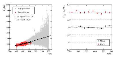
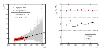
Figure 6: Examples of benchmark fit for the 750 m array. (Top panels) 1.00 < sec $\theta$ < 1.05. (Bottom panels) 1.15 < sec $\theta$ < 1.20. The solid (dashed) line corresponds to the fit done to the risetimes computed using the low-gain (high-gain) trace.

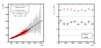
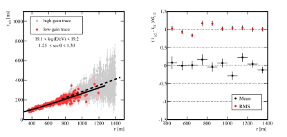
Figure 7: Examples of benchmark fit for the 1500 m array. (Top panels) 1.00 < sec $\theta$ < 1.05. (Bottom panels) 1.25 < sec $\theta$ < 1.30. The solid (dashed) line corresponds to the fit done to the risetimes computed using the low-gain (high-gain) trace.

In the right-hand plots of each pair, the mean and RMS deviations of the fits are seen to be consistent with 0 and 1, as expected for pull distributions r17 . The uncertainty in the axial distance has not been included in the fits as it is only around 2% for the distances in question.

Fits were made for A, B and $N(\theta)$ in six intervals of sec $\theta$ ranges 1.0 – 1.30 and 1.0 – 1.45 for the 750 m and 1500 m arrays respectively. In all six cases the $\chi^{2}$-values of the fits are between 1 and 1.2. To obtain the final parameterization of A, B and N as a function of $\theta$ fits have been made using the following functions

$$\begin{array}[]{l}A(\theta)=a_{0}+a_{1}(\sec\theta)^{-4}\\ B(\theta)=b_{0}+b_{1}(\sec\theta)^{-4}\\ N(\theta)=n_{0}+n_{1}(\sec\theta)^{2}+n_{2}e^{\sec\theta}\end{array}$$ (9)

where the seven coefficients, a_0, a₁ etc., are determined for the two arrays. This set of functions has been empirically chosen. It guarantees that, for the energy bins for which the benchmarks are defined, the mean value of $\Delta_{s}$ shows a flat behaviour as function of sec $\theta$. This naturally follows from the definition of $t_{\text{1/2}}^{\text{bench}}$. Since it embodies the dependence on sec $\theta$, the numerator in the definition of $\Delta_{i}$ has to be independent of the zenith angle.

We may thus define the benchmarks in terms of A, B and N as a function of sec $\theta$, enabling an appropriate benchmark to be defined for the zenith angle of the event under study. Thus $\Delta_{i}$ can be found for every station that satisfies the selection criterion and the corresponding value of $\Delta_{s}$ can be found for every selected event.

V Evolution of $\langle\Delta_{s}\rangle$ with energy and comparison with model predictions

We now describe the observed variation of $\langle$$\Delta_{s}$$\rangle$, the mean of $\Delta_{s}$ for a set of events, as a function of energy. The selection criteria for this analysis were presented in Table 2. The variation of $\langle$$\Delta_{s}$$\rangle$ with energy for the two arrays is shown in Fig. 8. Note that at the benchmark energies, indicated by the vertical bands, $\langle$$\Delta_{s}$$\rangle$ is zero, as expected by definition.

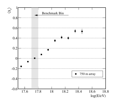
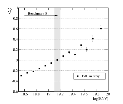
Figure 8: Evolution of $\langle$$\Delta_{s}$$\rangle$ as a function of energy for the two surface arrays: 750 m (left), 1500 m (right). The grey bands show the energy ranges where the benchmark functions were defined.

The results shown in Fig. 8 were obtained using the whole data set. We produce similar plots but this time splitting data in different bands of sec $\theta$. This exercise gives results that are consistent with the ones displayed in Fig. 8. Searches for anomalous behaviour of the largest, the second largest and the smallest signals separately have also been made: none was found.

To test the validity of hadronic models we can use $\langle$$\Delta_{s}$$\rangle$. In previous works r4 ; r5 ; r6 ; r7 strong evidence has been found that the models do not adequately describe the data and that the problem lies with the predictions of the muon content of showers. As the risetime is dominated by muons, $\langle$$\Delta_{s}$$\rangle$ is expected to provide a further investigation of this problem that will be useful because of the higher number of events and the extension to lower energies.

Libraries of simulations for the QGSJETII-04 r19 and EPOS-LHC r20 models and proton and iron primaries for zenith angles < 45^o and 17.5 < log (E/eV) < 20 have been created. In making comparisons with data it is necessary to choose which benchmarks to adopt. For consistency in what follows we use the benchmarks determined from data (section IV). Different choices of benchmarks would simply give shifts in the values of $\langle$$\Delta_{s}$$\rangle$, which would be the same for each data set.

For this study, the uncertainties in the risetimes have been found from simulations and adopting the ‘twins’ approach described in section III. The results are shown in Fig. 9 where it is seen that the uncertainties from the data are in good agreement with simulations using the QGSJETII-04 model at the benchmark energy.

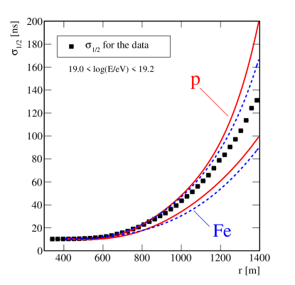
Figure 9: Risetime uncertainties estimated for protons (red lines), iron nuclei (blue dashed lines) and data as a function of core distance. For a clear view, the uncertainties corresponding to data are the average values. The uncertainties have been evaluated for events with energies in the range 19.0 < log (E/eV) < 19.2. The regions bracketed by the lines indicate the spread of the events simulated with QGSJETII-04 at a given distance.

A comparison of the evolution of $\langle$$\Delta_{s}$$\rangle$ with energy from the data with those from models is shown in Fig. 10.

The main sources that contribute to the systematic uncertainty are: a seasonal effect found when data are grouped according to the season of the year. It amounts to 0.03 for the 1500 m data and it is due to the variable conditions of pressure and temperature found in the atmosphere through the year. The UTC time at which the data were recorded also introduces a small uncertainty in our determination of $\langle$$\Delta_{s}$$\rangle$. Splitting data into periods corresponding to day and night, we obtain a value of this uncertainty of 0.01 for the 1500 m array data. Our observable also exhibits dependence with the ageing effects of surface detectors. We take as a systematic uncertainty the difference in $\langle$$\Delta_{s}$$\rangle$ found after grouping our data into two samples, one running from 2004 to 2010 and the other one from the years 2012 to 2014. For the 1500 m array, the difference amounts to 0.04. A small dependence of $\langle$$\Delta_{s}$$\rangle$ with sec $\theta$ is taken as source of systematics, its value being 0.02. Finally the systematic uncertainty associated to the energy scale ($\pm$14%) results in a systematic uncertainty on $\langle$$\Delta_{s}$$\rangle$ that amounts to 0.1. Adding all these contributions in quadrature, the overall systematic uncertainty in $\langle$$\Delta_{s}$$\rangle$ is 0.11 for the 1500 m array. A similar study for the 750 m array gives an overall systematic uncertainty in $\langle$$\Delta_{s}$$\rangle$ of 0.07. According to simulations, this is about 10% of the separation between proton and iron nuclei. It is evident, independent of which model is adopted, that the measurements suggest an increase of the mean mass with energy above $\sim$2.5 EeV if the hadronic models are correct.

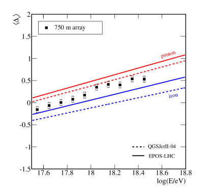
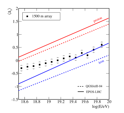
Figure 10: $\langle$$\Delta_{s}$$\rangle$ as a function of the energy for the two surface arrays. Brackets correspond to the systematic uncertainties. Data are compared to the predictions obtained from simulations.

Assuming the superposition model is valid and since $\langle$$\Delta_{s}$$\rangle$ is proportional to the logarithm of the energy (Fig. 8), the mean value of the natural logarithm of A (the atomic weight of an element) can be found from the following equation

$$\langle\ln A\rangle=\ln 56\frac{\langle\Delta_{s}\rangle_{\text{p}}-\langle\Delta_{s}\rangle_{\text{data}}}{\langle\Delta_{s}\rangle_{\text{p}}-\langle\Delta_{s}\rangle_{\text{Fe}}}$$ (10)

The results of this transformation for two models are shown in Fig. 11 and are compared with the Auger measurements of X_max made with the FD r21 . While the absolute values of $\langle$ln A$\rangle$ for the Delta method and the FD X_max differ from each other, the trend in $\langle$ln A$\rangle$ with energy is very similar. The observed difference arises because of the inadequate description of the muon component in the models used to get the $\langle$ln A$\rangle$ values. Notice that the electromagnetic cascade dominates the FD measurement whereas the Delta method is of a parameter that is a mixture of muons and the electromagnetic component. With substantially more events than in previous studies, we observe that the inconsistency between data and model predictions extends over a greater energy range than what was probed in past works.

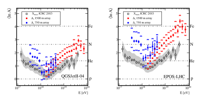
Figure 11: $\langle$ln A$\rangle$ as a function of energy for the Delta method and for X_max measurements done with the FD. QGSJetII-04 and EPOS-LHC have been used as the reference hadronic models. Statistical uncertainties are shown as bars. Brackets and shaded areas correspond to the systematic uncertainties associated to the measurements done with the SD and FD data, respectively.

In Fig. 12, the Delta results are also compared with the results of the analysis made using the asymmetry method r6 and with those from the study of the depth of muon production r4

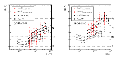
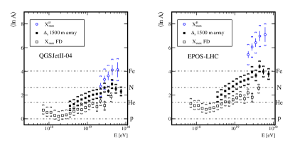
Figure 12: $\langle$ln A$\rangle$ as a function of the energy for analyses using FD data and SD data from the 1500 m array. QGSJetII-04 and EPOS-LHC have been used as the reference hadronic models. The results of the Delta method are compared with those arising from the asymmetry analysis r6 (top panels) and from the Muon Production Depth analysis r4 (bottom panels). Brackets correspond to the systematic uncertainties.

For EPOS-LHC the results from the asymmetry analysis, which is also based on risetimes and consequently on signals which are a mixture of the muon and the electromagnetic component, are in good agreement with the Delta results, albeit within the rather large statistical uncertainties. By contrast, the results from the MPD analysis, in which only muons are studied, give much larger (and astrophysically unexpected) values of $\langle$ln A$\rangle$. This once more indicates that the mechanisms of muon production in extensive air-showers are not properly described in current hadronic models.

VI Correlation of $\Delta_{s}$ with the Depth of Shower Maximum

We now address the correlation of $\Delta_{s}$ with the depth of shower maximum, X_max. As remarked earlier, we would not expect a 1:1 correlation between these parameters because the muon/electromagnetic mix incident on the water-Cherenkov detectors changes in a complex, but well-understood, manner with zenith angle, energy and distance. An idea of the correlation to be expected can be gained through Monte Carlo studies.

Values of $\Delta_{s}$ and X_max have been obtained from simulations of 1000 proton and 1000 iron nuclei showers made using the QGSJETII-04 model for the benchmark bin of the 1500 m array. The results are shown for three stations in Fig. 13. The fact that the Pearson’s correlation is less strong for Fe-nuclei than for protons, reflects the enhanced dominance of muons in showers initiated by Fe-primaries. The simulations give an indication of what is to be expected when the measurements of $\Delta_{s}$ are compared with the X_max values in the hybrid events for which the reconstruction of both observables is possible.

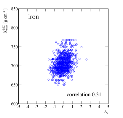
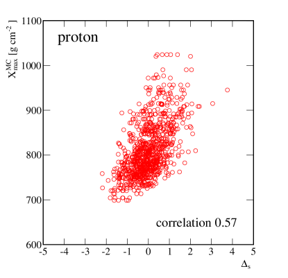
Figure 13: Pearson’s correlation of $\Delta_{s}$ and the true values of X_max for events simulated with QGSJETII-04 in the energy range 19.1 < log (E/eV) < 19.2. The left panel corresponds to iron nuclei; the right panel shows the correlation for protons. Values of $\Delta_{s}$ are computed for three stations.

To exploit the correlation using data, and hence extend the energy range and the statistical significance of the elongation rate determined with the FD, it is necessary to create empirical correlations using events in which both $\Delta_{s}$and X_max have been measured in the same events. For this study we used the data discussed in r1 for the 1500 m array for the events with energies > 3 EeV and a similar set of data from the 750 m array r21 for events of lower energy. The selection of events is shown in Table 3.

Table 3: Set of cuts used to select events simultaneously reconstructed by the fluorescence and surface detectors. These events are used for calibration purposes. $\epsilon$ stands for the overall efficiency. HEAT data are obtained with a set of three fluorescence detectors that point to the higher zenith angles appropriate to the lower energies.

750 m array			1500 m array
Quality cuts	Events	$\epsilon$ (%)	Quality cuts	Events	$\epsilon$ (%   )
HEAT data	12 003	100.0	FD data	19 759	100.0
FD & SD recon	2 461	20.5	FD & SD recon	12 825	65.0
sec $\theta$ < 1.30	2 007	16.7	sec $\theta$ < 1.45	9 625	49.0
6T5 trigger	714	5.9	6T5 trigger	7 361	37.0
$\geq$ 3 selected stations	660	5.5	$\geq$ 3 selected stations	4 025	20.0
log (E/eV) $\geq$ 17.5	252	2.1	log (E/eV) $\geq$ 18.5	885	4.5

The $\Delta_{s}$and X_max of the events selected for the purposes of calibration are shown for the two arrays in Fig. 14. There are 252 and 885 events for the 750 m and 1500 m arrays respectively available for calibration of which 161 have energies >10 EeV. The small number for the 750 m array reflects the shorter period of operation and the relatively small area (23.5 km²) of the array. We have checked that the sample of events selected is unbiased by comparing the elongation rate determined from the full data set (from HEAT and standard fluorescence telescopes) with that found from the 252 and 885 events alone.

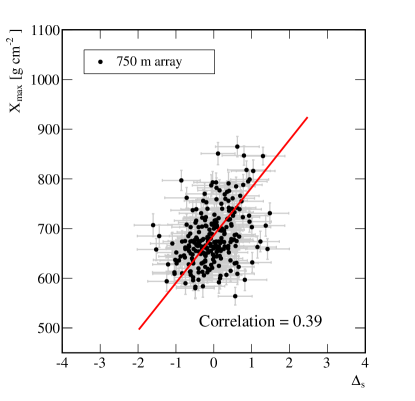
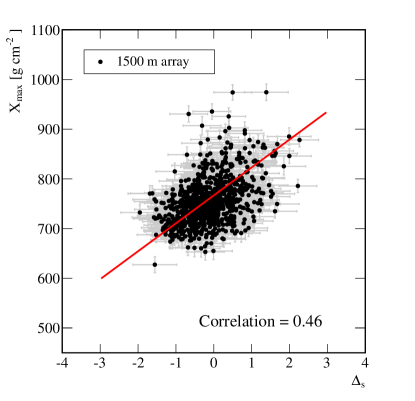
Figure 14: (Left) Correlation of X_max and $\Delta_{s}$ for the 252 events from the 750 m array. (Right) Correlation of X_max and $\Delta_{s}$for the 885 events of the 1500 m array.

Table 4: Coefficients obtained from the calibration of $\Delta_{s}$ and X_max.

	750 m array	1500 m array
Calibration parameters	Value (g cm-2)	Value (g cm -2)
a	636 $\pm$ 20	699 $\pm$ 12
b	96 $\pm$ 10	56 $\pm$ 3
c	2.9 $\pm$ 1.2	3.6 $\pm$ 0.7

For the calibration we fit functions of the form

$$X_{\text{max}}=a+b\Delta_{s}+c\log(E/\text{eV})$$ (11)

to the two data sets. The term ‘b’ is dominant in the fit. The term ‘c’ is included to accommodate the energy dependence of both variables. A fit including a quadratic term in log (E/eV) does not modify our results. The uncertainties in X_max are taken from r1 . We have used the maximum likelihood method to make the fits which give the coefficients listed in Table 4. The three coefficients are not independent. Their Pearson’s correlations are $\rho_{ab}$=-0.2, $\rho_{ac}$=-0.97 and $\rho_{bc}$=0.34. These correlations are taken into account when evaluating the systematic uncertainty associated with the calibration procedure.

We have also evaluated the systematic uncertainties associated with the measurements of X_max deduced from the surface detectors. These include the seasonal, diurnal, ageing and $\theta$ dependence already discussed for $\langle$$\Delta_{s}$$\rangle$ in section V that X_max propagate to our measurement. Now two further sources of systematic arise. One is related to the uncertainty in the calibration parameters. We have propagated this uncertainty taking into account the correlation of the parameters a, b and c. For the 1500 m array, the differences in X_max span from 3 g cm^-2 at the lowest energies to 5 g cm^-2 at the upper end of the energy spectrum. We quote conservatively as a systematic uncertainty the largest value found and consider it constant for the whole energy range. A similar procedure for the 750 m array data results on a systematic uncertainty of 10 g cm^-2. The systematic uncertainty obtained in the measurement of X_max with the FD detector propagates directly into the values obtained with the SD data. In r1 the systematic uncertainty is given as a function of the energy. In this analysis, the average of those values is quoted a systematic uncertainty that is constant with energy. The values are shown for each effect and for each array in Table 5.

The systematic uncertainties have been added in quadrature to give 14 and 11 g cm^-2 for the 750 and 1500 m arrays respectively.

The values of X_max found from this analysis are shown as a function of energy in Fig. 15. The resolution in the measurement of X_max with the surface detector data is 45 g cm^-2.

Table 5: Breakdown of the systematic uncertainties of X_max for the 750 m and 1500 m arrays. The systematic uncertainty obtained in the measurement of X_max with the FD and HEAT detectors propagates directly into the values obtained with the SD data. The rest of systematic uncertainties quoted in this table are intrinsic to the Delta method.

750 m array		1500 m array
Source	Systematic uncertainty (g cm-2)	Source	Systematic uncertainty (g cm-2)
Uncertainty on calibration	10.0	Uncertainty on calibration	5.0
Seasonal effect	2.0	Seasonal effect	2.0
Diurnal dependence	1.0	Diurnal dependence	1.0
Ageing	3.0	Ageing	3.0
HEAT systematic uncertainty	8.5	FD systematic uncertainty	8.5
Angular dependence	<1.0	Angular dependence	1.5
Total	14.0	Total	11.0

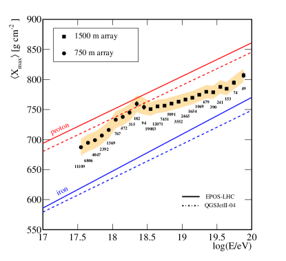
Figure 15: Mean values of the X_max distributions obtained with the data of the 750 m and 1500 m surface arrays as a function of the energy. The shaded area indicates the systematic uncertainties. Data are compared to the predictions from simulations of protons and iron nuclei for two different hadronic models. The number of selected events in each energy bin is indicated.

In Fig. 16 measurements in the region of overlap between the two arrays are shown. The agreement is satisfactory.

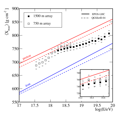
Figure 16: Same as Fig. 15 including additional X_max measurements from the surface detectors above and below 3 EeV. (Inset) Three energy bins have been included below 3 EeV using the data of the 1500 m array and two measurements added above 3 EeV use the data of the 750 m array. There is good agreement between measurements in the overlap region. The brackets correspond to systematic uncertainties.

In Fig. 17 the data of Fig. 15 are compared with measurements made with the fluorescence detectors [21].

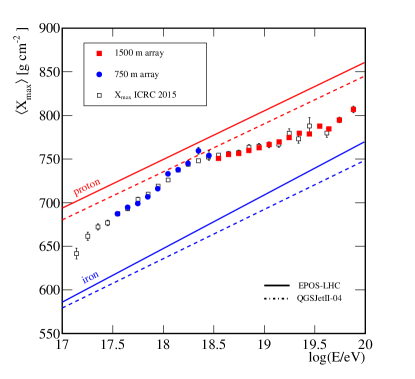
Figure 17: Evolution of $\langle$X_max$\rangle$ as a function of energy. The figure compares the mean values of the X_max distributions measured by the fluorescence and surface detectors of the Pierre Auger Observatory. In most cases the uncertainties are smaller than the size of the symbols.

The agreement is good: the results from the surface detector alone are statistically stronger and extend to higher energies.

VI.1 Interpretation of the measurements in terms of average mass

A comparison with hadronic models allows the expression of the average depth of shower maxima in terms of the natural logarithm of the atomic mass $\langle$ln A$\rangle$, following the procedure discussed in section V. The evolution of $\langle$ln A$\rangle$ as a function of energy is shown in Fig. 18. In the energy range where the FD and SD measurements coincide, the agreement is good. For both hadronic models the evolution of $\langle$ln A$\rangle$ with energy is similar. However the EPOS-LHC model suggests a heavier average composition. SD measurements have been used to confirm, with a larger data set, what has already been observed with FD measurements, namely that the primary flux of particles is predominantly composed of light particles at around 2 EeV and that the average mass increases up to $\sim$40 EeV. Above this energy, the SD measurements can be used to draw inferences about mass composition with good statistical power. The last two bins indicate a possible change in the dependence of X_max with energy above 50 EeV, with the final point lying $\sim$3 sigma above the elongation rate fitted to data above 3 EeV. It is, therefore, possible that the increase of the primary mass with energy is slowing at the highest energies but we need to reduce statistical and systematic uncertainties further before strong conclusions can be drawn. AugerPrime, the upgrade of the surface-detector array of the Pierre Auger Observatory r22 , will significantly improve our capability to elucidate mass composition on an event-by-event basis in the energy range of the flux suppression.

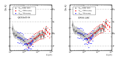
Figure 18: $\langle$ln A$\rangle$ as a function of the energy. QGSJetII-04 and EPOS-LHC have been used as the reference hadronic models. The results of the Delta method are compared with those based on X_max measurements done with the FD r21 . Brackets and shaded areas correspond to the systematic uncertainties; bars correspond to uncertainties of statistical nature.

VII Summary and Conclusions

We have described a new method for extracting relevant information from the time profiles of the signals from the water-Cherenkov detectors of the Pierre Auger Observatory. With it, we have been able to obtain information on the evolution of the mean depth of shower maximum with energy over a larger energy range than has been studied previously using over 81,000 events of which 123 are of energy >50 EeV. We have also been able to expand the discussions of the mismatch between data and predictions from models based on extrapolations of hadronic interactions from LHC energies. Specifically we have reported the following:

1. The comparison of the risetime data with fluorescence measurements reinforces the conclusions reported previously r4 ; r5 ; r6 ; r7 that the modelling of showers provides an inadequate description of air-shower data. The deductions are made over a larger energy range and with smaller statistical uncertainties than hitherto (Fig. 11 and Fig. 12).

2. The depth of shower maximum has been measured from 0.3 EeV to 100 EeV using data of the Surface Detector (Fig. 15).

3. Data from the 750 m array of the Observatory have been used to derive mass information for the first time.

4. The mean measurements of X_max have been compared with predictions from the EPOS-LHC and QGSJetII04 models and estimates of $\langle$ln A$\rangle$ extracted (Fig. 18). While the EPOS-LHC model leads to larger values of $\langle$ln A$\rangle$ than are found with the other model, both show the general trend of the mean mass becoming smaller as the energy increases up to $\sim$2 EeV, after which it rises slowly with energy up to about 50 EeV where this rise seems to stop.

Appendix A: Data Tables

Table A1: Values of $\langle$$\Delta_{s}$$\rangle$ for the 750 m array. The fourth column shows the statistical uncertainty. For all measurements the systematic uncertainty amounts to 0.07.

Log (E/eV) range	$\langle$Log (E/eV) $\rangle$	$\langle$$\Delta_{s}$$\rangle$	$\sigma$stat($\langle$$\Delta_{s}$$\rangle$)
[17.5,17.6)	17.55	-0.157	0.009
[17.6,17.7)	17.65	-0.064	0.009
[17.7,17.8)	17.75	0.004	0.008
[17.8,17.9)	17.85	0.077	0.011
[17.9,18.0)	17.95	0.170	0.014
[18.0,18.1)	18.05	0.35	0.02
[18.1,18.2)	18.15	0.41	0.03
[18.2,18.3)	18.25	0.40	0.03
[18.3,18.4)	18.35	0.54	0.03
[18.4,18.5)	18.45	0.53	0.05

Table A2: Values of $\langle$$\Delta_{s}$$\rangle$ for the 1500 m array. The fourth column shows the statistical uncertainty. For all measurements the systematic uncertainty amounts to 0.11.

Log (E/eV) range	$\langle$Log (E/eV) $\rangle$	$\langle$$\Delta_{s}$$\rangle$	$\sigma$stat($\langle$$\Delta_{s}$$\rangle$)
[18.5,18.6)	18.55	-0.297	0.005
[18.6,18.7)	18.65	-0.242	0.006
[18.7,18.8)	18.75	-0.218	0.007
[18.8,18.9)	18.85	-0.163	0.009
[18.9,19.0)	18.95	-0.108	0.011
[19.0,19.1)	19.05	-0.056	0.012
[19.1,19.2)	19.15	0.004	0.015
[19.2,19.3)	19.25	0.077	0.020
[19.3,19.4)	19.35	0.15	0.03
[19.4,19.5)	19.45	0.11	0.03
[19.5,19.6)	19.55	0.29	0.04
[19.6,19.7)	19.64	0.20	0.04
[19.7,19.8)	19.74	0.41	0.06
[19.8,$\infty$)	19.88	0.60	0.06

Table A3: Values of $\langle$X_max$\rangle$ for the 750 m array. The fourth column shows the statistical uncertainty. For all measurements the systematic uncertainty amounts to 14 g cm^-2.

Log (E/eV) range	$\langle$Log (E/eV) $\rangle$	$\langle$Xmax/ g cm-2$\rangle$	$\sigma$stat($\langle$Xmax$\rangle$)/g cm-2
[17.5,17.6)	17.55	687.2	0.5
[17.6,17.7)	17.65	695.6	0.6
[17.7,17.8)	17.75	699.9	0.8
[17.8,17.9)	17.85	707	1.0
[17.9,18.0)	17.95	716	1.0
[18.0,18.1)	18.05	733	2.0
[18.1,18.2)	18.15	738	3.0
[18.2,18.3)	18.25	745	3.0
[18.3,18.4)	18.35	759	4.0
[18.4,18.5)	18.45	754	5.0

Table A4: Values of $\langle$X_max$\rangle$ for the 1500 m array. The fourth column shows the statistical uncertainty. For all measurements the systematic uncertainty amounts to 11 g cm^-2.

Log (E/eV) range	$\langle$Log (E/eV) $\rangle$	$\langle$Xmax/ g cm-2$\rangle$	$\sigma$stat($\langle$Xmax$\rangle$) /g cm-2
[18.5,18.6)	18.55	750.7	0.3
[18.6,18.7)	18.65	755.2	0.3
[18.7,18.8)	18.75	756.4	0.4
[18.8,18.9)	18.85	759.8	0.6
[18.9,19.0)	18.95	763.0	0.6
[19.0,19.1)	19.05	766.5	0.7
[19.1,19.2)	19.15	769.6	0.9
[19.2,19.3)	19.25	775	1.0
[19.3,19.4)	19.35	780	2.0
[19.4,19.5)	19.45	779	2.0
[19.5,19.6)	19.55	788	2.0
[19.6,19.7)	19.64	785	2.0
[19.7,19.8)	19.74	795	3.0
[19.8,$\infty$)	19.88	807	3.0

References

- (1) A. Aab et al. [Pierre Auger Collaboration], Phys. Rev. D 90, 122005 (2014) [arXiv:1409.4809 [astro-ph.HE]].
- (2) R. U. Abbasi et al., Astropart. Phys. 64, 49 (2015) [arXiv:1408.1726 [astro-ph.HE]].
- (3) A. Aab et al. [Pierre Auger Collaboration], Phys. Rev. D 90, 122006 (2014) [arXiv:1409.5083 [astro-ph.HE]].
- (4) A. Aab et al. [Pierre Auger Collaboration], Phys. Rev. D 90, 012012 (2014) Addendum: [Phys. Rev. D 90, 039904 (2014)] Erratum: [Phys. Rev. D 92, 019903 (2015)] [arXiv:1407.5919 [hep-ex]].
- (5) A. Aab et al. [Pierre Auger Collaboration], Phys. Rev. D 91, 032003 (2015) Erratum: [Phys. Rev. D 91, 059901 (2015)] [arXiv:1408.1421 [astro-ph.HE]].
- (6) A. Aab et al. [Pierre Auger Collaboration], Phys. Rev. D 93, 072006 (2016) [arXiv:1604.00978 [astro-ph.HE]].
- (7) A. Aab et al. [Pierre Auger Collaboration], Phys. Rev. Lett. 117, 192001 (2016) [arXiv:1610.08509 [hep-ex]].
- (8) A. Aab et al. [Pierre Auger Collaboration], Nucl. Instrum. Meth. A 798, 172 (2015) [arXiv:1502.01323 [astro-ph.IM]].
- (9) X. Bertou et al. [Pierre Auger Collaboration], Nucl. Instrum. Meth. A 568, 839 (2006).
- (10) J. Abraham et al. [Pierre Auger Collaboration], Nucl. Instrum. Meth. A 613, 29 (2010) [arXiv:1111.6764 [astro-ph.IM]].
- (11) D. Newton, J. Knapp, A.A. Watson, Astropart.Phys. 26, 414 (2007).
- (12) J. Abraham et al. [Pierre Auger Collaboration], Phys. Rev. Lett. 101, 061101 (2008) [arXiv:0806.4302 [astro-ph]].
- (13) V. Verzi, PoS ICRC 2015, 015 (2016).
- (14) A. A. Watson and J. G. Wilson, J. Phys. A 7, 1199 (1974).
- (15) J. Linsley and L. Scarsi, Phys. Rev. 128, 2384 (1962).
- (16) A. J. Baxter, J. Phys. A 2, 50 (1969).
- (17) K. Greisen, Ann. Rev. Nucl. Part. Sci. 10, 63 (1960).
- (18) L. Demotier and L. Lyons, CDF/ANAL/PUBLIC/5776, 2002.
- (19) Pierre Auger Collaboration in preparation.
- (20) S. Ostapchenko, Phys. Rev. D 83, 014018 (2011) [arXiv:1010.1869 [hep-ph]].
- (21) T. Pierog, I. Karpenko, J. M. Katzy, E. Yatsenko and K. Werner, Phys. Rev. C 92, 034906 (2015) [arXiv:1306.0121 [hep-ph]].
- (22) A. Porcelli for the Pierre Auger Collaboration, PoS (ICRC2015) 420.
- (23) A. Aab et al. [Pierre Auger Collaboration], arXiv:1604.03637 [astro-ph.IM].