Conserved Charges in Extended Theories of Gravity

Abstract

We give a detailed review of construction of conserved quantities in extended theories of gravity for asymptotically maximally symmetric spacetimes and carry out explicit computations for various solutions. Our construction is based on the Killing charge method, and a proper discussion of the conserved charges of extended gravity theories with this method requires studying the corresponding charges in Einstein’s theory with or without a cosmological constant. Hence we study the ADM charges (in the asymptotically flat case but in generic viable coordinates), the AD charges (in generic Einstein spaces, including the anti-de Sitter spacetimes) and the ADT charges in anti-de Sitter spacetimes. We also discuss the conformal properties and the behavior of these charges under large gauge transformations as well as the linearization instability issue which explains the vanishing charge problem for some particular extended theories. We devote a long discussion to the quasi-local and off-shell generalization of conserved charges in the 2+1 dimensional Chern-Simons like theories and suggest their possible relevance to the entropy of black holes.

Contents

1. I Reading Guide and Conventions
2. I GLOBAL CONSERVED CHARGES
   1. II Introduction
   2. III ADT Energy
      1. III.1 AD and ADM Conserved Charges
      2. III.2 Large diffeomorphisms (gauge transformations)
      3. III.3 Schwarzschild-(A)dS Black Holes in $n$-dimensions
      4. III.4 Kerr-AdS Black Holes in $n$-dimensions
      5. III.5 Computation of the charges for the solitons
         1. III.5.1 The $AdS$ Soliton
         2. III.5.2 Eguchi-Hanson Solitons
      6. III.6 Energy of the Taub-NUT-Reissner-Nordstr$\ddot{\text{o}}$m metric
   3. IV Charges of Quadratic Curvature Gravity
   4. V Charges of $f\left(R_{\rho\sigma}^{\mu\nu}\right)$ Gravity
      1. V.1 Example 1: Charges of Born-Infeld Extension of New Massive Gravity (BINMG)
   5. VI Conserved Charges of Topologically Massive Gravity
      1. VI.0.1 Logarithmic solution of TMG at the chiral point
      2. VI.0.2 Null warped AdS₃
      3. VI.0.3 Spacelike stretched black holes
   6. VII Charges in Scalar-Tensor Gravities
   7. VIII Conserved Charges in the First Order Formulation
   8. IX Vanishing Conserved Charges and Linearization Instability
3. II CONSERVED CHARGES FOR EXTENDED 3D GRAVITIES: QUASI-LOCAL APPROACH
   1. X Introduction
   2. XI Chern-Simons-like theories of gravity
      1. XI.1 First order formalism of gravity theories
      2. XI.2 Lorentz-Lie derivative and total variation
      3. XI.3 Gravity in three dimensions
      4. XI.4 Chern-Simons-like theories of gravity as the general
   3. XII Some examples of Chern-Simons-like theories of gravity
      1. XII.1 Example.1: Einstein’s gravity with a negative cosmological constant
         1. XII.1.1 Banados-Teitelboim-Zanelli black hole
      2. XII.2 Example.2: Minimal Massive Gravity
      3. XII.3 Example.3: New Massive Gravity
         1. XII.3.1 Rotating Oliva-Tempo-Troncoso black hole as a solution of new massive gravity
      4. XII.4 Example.4: Generalized Massive Gravity
      5. XII.5 Example.5: Generalized Minimal Massive Gravity
         1. XII.5.1 Solutions of Einstein gravity with negative cosmological constant
         2. XII.5.2 Warped black holes
   4. XIII Extended off-shell ADT current
   5. XIV Off-shell extension of the covariant phase space method
   6. XV Quasi-local conserved charge
   7. XVI Black hole entropy in Chern-Simons-like theories of gravity
   8. XVII Asymptotically AdS₃ spacetimes
      1. XVII.1 Brown-Henneaux boundary conditions
      2. XVII.2 General massive gravity
   9. XVIII Asymptotically spacelike warped anti-de Sitter spacetimes in General Minimal Massive Gravity
      1. XVIII.1 Asymptotically spacelike warped AdS₃ spacetimes
      2. XVIII.2 Conserved charges of asymptotically spacelike warped AdS₃ spacetimes in General Minimal Massive Gravity
      3. XVIII.3 The algebra of conserved charges
      4. XVIII.4 Mass, angular momentum and entropy of warped black hole solution of general minimal massive Gravity
   10. XIX Conserved charges of the Rotating Oliva-Tempo-Troncoso black hole
   11. XX Explicit examples of the black hole entropy
       1. XX.1 Banados-Teitelboim-Zanelli black hole entropy
          1. XX.1.1 Minimal Massive Gravity
          2. XX.1.2 General Massive Gravity
          3. XX.1.3 General Minimal Massive Gravity
       2. XX.2 Warped black hole entropy from the gravity side
       3. XX.3 Entropy of the rotating Oliva-Tempo-Troncoso black hole
   12. XXI Near horizon symmetries of the non-extremal black hole solutions of the General Minimal Massive Gravity
       1. XXI.1 Near horizon symmetries of non-extremal black holes
       2. XXI.2 Near horizon conserved charges and their algebra for General Minimal Massive Gravity
   13. XXII Extended near horizon geometry
       1. XXII.1 Application to the general minimal massive gravity
       2. XXII.2 Soft hair and the soft hairy black hole entropy
   14. XXIII Horizon Fluffs In Generalized Minimal Massive Gravity
       1. XXIII.1 "Asymptotic" and "near horizon" conserved charges and their algebras
          1. XXIII.1.1 Asymptotic conserved charges
          2. XXIII.1.2 Near horizon conserved charges
       2. XXIII.2 Relation between the asymptotic and near horizon algebras
   15. XXIV Asymptotically flat spacetimes in General Minimal Massive Gravity
       1. XXIV.1 Asymptotically 2+1 Dimensional Flat Spacetimes
       2. XXIV.2 Conserved charges of asymptotically flat spacetimes in general minimal massive gravity
       3. XXIV.3 Thermodynamics
   16. XXV Conserved Charges of Minimal Massive Gravity Coupled to Scalar Field
       1. XXV.1 Minimal massive gravity coupled to a scalar field
       2. XXV.2 Field equations
       3. XXV.3 Quasi-local conserved charges
       4. XXV.4 General formula for entropy of black holes in minimal massive gravity coupled to a scalar field
       5. XXV.5 Application for the BTZ black hole with $\varphi=\varphi_{0}$
       6. XXV.6 Virasoro algebra and the central extension
   17. XXVI Conclusions
   18. XXVII Acknowledgments
   19. A EQCA and Linearization of the Field Equations
   20. B Procedure of obtaining equations (331)-(336)
   21. C Technical proof of equation (338)

I Reading Guide and Conventions

This review is naturally divided into two parts: In Part I, we discuss global conserved charges for generic modified or extended gravity theories. Global here refers to the fact that the integrals defining the charges are on a spacelike surface on the boundary of the space. In Part II, we discuss quasi-local and off-shell conserved charges; particularly, for 2+1 dimensional gravity theories with Chern-Simons like actions. In what follows, the meaning of these concepts will be elaborated. Here, let us briefly denote our conventions of the signature of the metric and the Riemann curvature: We use the mostly plus signature with $g=\text{diag}(-,+,...,+)$ and take the Riemann tensor to be defined as

$$\left[\nabla_{\mu},\nabla_{\nu}\right]V^{\rho}=R_{\mu\nu\phantom{\rho}\sigma}^{\phantom{\mu\nu}\rho}V^{\sigma},$$ (1)

and the Ricci tensor is defined as

$$R_{\mu\nu}=R_{\phantom{\rho}\mu\rho\nu}^{\rho},$$ (2)

while the scalar curvature is

$$R=R_{\phantom{\mu}\mu}^{\mu}.$$ (3)

Part I GLOBAL CONSERVED CHARGES

II Introduction

The first “casualty of gravity” is Noether’s theorem Noether , well at least for the case of rigid spacetime symmetries and their corresponding conserved charges. The “Equivalence Principle” in any form is both a blessing and a curse: it makes gravity locally trivial (essentially a coordinate effect in the extreme limit of going to a point-like lab) but then it also, for the same reason, makes it hard to find local observables in gravity. In fact all the observables must be global. To heuristically understand this, as an example, consider the energy momentum density of the gravitational field: Being a bosonic (spin-2) field, its kinetic energy density is expected to be of the form $K\sim\partial g\partial g$ which makes no covariant sense as it can be set to zero in a locally inertial frame (or in Riemann normal coordinates). This state of affairs of course affects both the classical gravity and the would-be quantum gravity. The first thing one wants to know and compute in any theory are the “observables” and it turns out generically, a spacetime has no observables and it would not make sense to construct classical and quantum theories for those spacetimes. For example, in a spacetime such as the de Sitter spacetime which does not have a global timelike Killing vector or an asymptotic spatial infinity, defining a global conserved positive energy is not possible Witten_dS .

In the absence of a tensorial quantity that can represent local gravitational energy-mass, momentum etc, one necessarily resorts to new ideas; two of which are quasilocal expressions that try to capture gravitational quantities contained in a finite region of space or the global expressions that are assigned to the totality of spacetime. Both of these involve integrations over some regions of space, and they are not tensorial. But, that does not mean that they are physically irrelevant. On the contrary, they are designed to answer physical questions such as what is the mass of a black hole or how much energy is radiated if two black holes merge as in the recent observations by the LIGO detectors, of course with the assumption that these systems can be isolated from the rest of the Universe? Especially, global expressions that we shall discuss, the Arnowitt-Deser-Misner (ADM) adm and the Abbott-Deser (AD) conserved charges Abbott , and their generalizations to higher derivative models the Abbott-Deser-Tekin (ADT) conserved charges Deser_Tekin-PRL ; Deser_Tekin-PRD are well-defined for asymptotically flat and anti-de Sitter spaces, given the proper decay conditions on the metric and the extrinsic curvature of the Cauchy surface.

The celebrated ADM mass assigned to an asymptotically flat manifold exactly coincides with our expectation of an isolated gravitational system’s mass, such as the mass of a black hole. It also turns out that the ADM mass is a geometric invariant of an asymptotically flat Riemannian manifold as long as the proper decay conditions are satisfied Bartnik . It is interesting to note that the ADM mass of an asymptotically flat manifold also became an important part of differential geometry and it took a long time by differential geometers to prove the positiveness of this quantity (under certain assumptions) as was expected to be positive from the physical arguments such as the stability of the Minkowski spacetime, or supergravity arguments which require the Hamiltonian to be positive definite. An account of these discussions as well as a review of the conserved charges in Einstein’s theory can be found in the relevant chapters of the book Ashtekar .

After the series of ADM papers, whose results were summarized in adm a great deal of effort was devoted to better understand the Hamiltonian structure of gravity theories. The literature is too great to do any justice here; but several works stand out which we now briefly note: Regge and Teitelboim Regge:1974zd realized that the Hamiltonian of general relativity on a space with a boundary does not have well-defined functional derivatives; therefore, Hamilton’s equations for the phase space fields are not equal to the Euler-Lagrange equations. Their detailed analysis shows that the remedy is to add a boundary term, and that boundary term is exactly the ADM mass of the asymptotically flat spacetime. This approach is rather revolutionary for two reasons: first naively, due to the constraints, the bulk Hamiltonian vanishes exactly in general relativity; and therefore, if one does not add a boundary term the spacetime is devoid of any energy. On the other hand, once a boundary term is added, the full Hamiltonian when evaluated on-shell reduces to the boundary term. Thus, the numerical value of the total Hamiltonian is the ADM energy. Secondly, the ADM energy, even though it looks linear in the metric (deviation) at infinity, captures all the nonlinear energy in the bulk. This is evident from the Regge-Teitelboim approach.

The next generalization was that of the AD Abbott mass for asymptotically de Sitter or anti-de Sitter spacetimes. In fact, Abbott and Deser were interested in the stability of the de Sitter spacetime; however, the AD expression is also well-defined for anti-de Sitter (AdS) spacetimes which have a spatial infinity at which the surface integrals can be defined in a coordinate invariant manner. Following the Regge-Teitelboim Regge:1974zd , the extension of the Hamiltonian approach to the anti-de Sitter spacetime was given bu Henneaux and Teitelboim in hen84 , and more recently in jamsin which also includes relevant references.

The next development, which is the main focus of this review, was the construction of conserved charges in generic higher curvature theories in various dimensions using the AD methods. These higher derivative theories picked up interest due to their potential to behave better at high and low energies where Einstein’s gravity suffer; hence, the construction of conserved quantities in these theories became important. The Hamiltonian treatment following Regge:1974zd ; hen84 in the extended gravity theories is highly complicated due to their higher derivative nature. On the other hand, the AD approach is relatively straightforward. Deser and Tekin Deser_Tekin-PRL ; Deser_Tekin-PRD extended the AD Killing charge construction for gravity theories that have quadratic or more powers in spacetimes which are asymptotically AdS. It is important to understand that the cosmological constant plays a crucial role in all these conserved quantities. For example, generically for a nonzero cosmological constant $\Lambda$, a term in the action of the form $\alpha\left({\rm Riem}\right)^{n}$ contributes to the conserved charges as much as $\alpha\Lambda^{n-1}$ times the Einstein’s theories contribution. Therefore, a given spacetime might have quite different conserved quantities in different theories.

We would like make one disclaimer before we lay out the computations leading to the conserved quantities in generic gravity theories: our basic tool is the Killing charge construction as employed most clearly in Abbott ; Deser_Tekin-PRD . As our main focus is generic higher derivative theories, the review basically evolves around the AD work and its extension the ADT work. Of course there are other approaches to the same problem which we have not followed here such as the works of Magnon ; HawkingHorowitz ; 97 ; Aros ; 40 ; elsewhere comparisons of various methods are discussed in detail; see for example Hollands by Hollands, Ishibashi and Marolf. For a recent review on conserved charge and related topics in general relativity, please see Tekin_et_al , Banados_rev , and Compere .

III ADT Energy

Let us consider a generic gravity theory defined by the field equations

$$\mathcal{E}_{\mu\nu}\left(g,R,\nabla R,R^{2},...\right)=\kappa\tau_{\mu\nu},$$ (4)

where $\mathcal{E}_{\mu\nu}$ is a divergence-free, symmetric two-tensor possibly coming from an action. Here, $R$ denotes the Riemann tensor or its contractions, $\kappa$ is the $n$-dimensional Newton’s constant and $\tau_{\mu\nu}$ represents the nongravitational matter source. It is clear that $\nabla_{\mu}\mathcal{E}^{\mu\nu}=0$ does not yield a globally conserved charge without further structure. A moment of reflection shows that given an exact Killing vector $\xi^{\mu}$, one can construct a covariantly-conserved current $J^{\mu}:=\xi_{\nu}\mathcal{E}^{\mu\nu}$ yielding a partially-conserved current density $\mathcal{J}^{\mu}:=\sqrt{-g}\xi_{\nu}\mathcal{E}^{\mu\nu}$ since $\partial_{\mu}\left(\sqrt{-g}\xi_{\nu}\mathcal{E}^{\mu\nu}\right)=\sqrt{-g}\nabla_{\mu}\left(\xi_{\nu}\mathcal{E}^{\mu\nu}\right)=0$. But, as this current identically vanishes outside the sources, it does not lead to a physically meaningful nontrivial conserved quantity. The compromise is to follow the ADM construction for asymptotically flat geometries, and AD and ADT constructions for asymptotically (anti-)de Sitter [(A)dS] geometries, and split the metric into a background $\bar{g}_{\mu\nu}$ and a fluctuation $h_{\mu\nu}$ as

$$g_{\mu\nu}=\bar{g}_{\mu\nu}+\kappa h_{\mu\nu}.$$ (5)

Here and in what follows, without worrying about the units of $\kappa$, we shall use it as a perturbation order counting parameter. Clearly, the decomposition of the metric $g$ as (5) is coordinate dependent, and hence a different set of coordinates would lead to different $\bar{g}_{\mu\nu}$ and $h_{\mu\nu}$ tensors. But, it is a simple exercise to show that infinitesimal change of coordinates on the manifold can be seen as a gauge transformation of the form $h_{\mu\nu}^{\prime}\left(x\right)=h_{\mu\nu}\left(x\right)+\bar{\nabla}_{\mu}\zeta_{\nu}\left(x\right)+\bar{\nabla}_{\nu}\zeta_{\mu}\left(x\right)$ where $\bar{\nabla}_{\mu}$ and all the barred quantities refer to the background metric $\bar{g}_{\mu\nu}$. Therefore, $h_{\mu\nu}$ in this setting is a background two-tensor. At this stage, even though $\bar{g}_{\mu\nu}$ is defined by the equation

$$\mathcal{E}_{\mu\nu}\left(\bar{g},\bar{R},\bar{\nabla}\bar{R},\bar{R}^{2},...\right)=0,$$ (6)

clearly there is a still a large and perhaps infinite degeneracy in the choice of the background metric. In principle any solution of the above equation can be taken as a background and we will consider any Einstein metric as a background in Einstein’s theory; however, in a generic gravity theory obtaining nontrivial solutions is itself an outstanding problem; therefore, in what follows we will choose the background to be a maximally symmetric spacetime for which the complicated field equations of a generic gravity theory highly simplify and yield a solution. Thus, we will make this choice, and often refer to $\bar{g}$ to be the (classical) vacuum with the following properties

$$\bar{R}_{\mu\alpha\nu\beta}=\frac{2}{\left(n-2\right)\left(n-1\right)}\Lambda\left(\bar{g}_{\mu\nu}\bar{g}_{\alpha\beta}-\bar{g}_{\mu\beta}\bar{g}_{\alpha\nu}\right),\qquad\bar{R}_{\mu\nu}=\frac{2}{n-2}\Lambda\bar{g}_{\mu\nu},\qquad\bar{R}=\frac{2n\Lambda}{n-2}.$$ (7)

Inserting these into (6), one arrives at an equation $f\left(\Lambda\right)\bar{g}_{\mu\nu}=0$ which determines the effective cosmological constant $\Lambda$. Of course, depending on the parameters of the theory, there could be no real-valued solution or many solutions. The case of no maximally symmetric solution is an interesting one which we shall not discuss here. If there are many real-valued solutions for $\Lambda$, at this stage there is no compelling reason to choose one over the other. Therefore, any such vacuum would be viable. Hence, as far as the charge construction is concerned, we shall simply consider a generic $\Lambda$ which is a real-valued solution to the vacuum equation (6). Once such a $\Lambda$ exists, there are $n\left(n+1\right)/2$ background Killing symmetries which we shall collectively denote as $\bar{\xi}_{a}^{\mu}$. But, not to clutter the notation we will simply omit the index $a$.

The splitting (5) as applied to the field equations (4) yields

$$\mathcal{E}_{\mu\nu}\left(\bar{g}\right)+\kappa\mathcal{E}_{\mu\nu}^{\left(1\right)}\left(h\right)+\kappa^{2}\mathcal{E}_{\mu\nu}^{\left(2\right)}\left(h\right)+O\left(\kappa^{3}\right)=\kappa\tau_{\mu\nu}.$$ (8)

We can move all the nonlinear terms to the right-hand side and recast the equation as a linear operator in $h$ with a nontrivial source term that includes not only the matter source, but also the gravitational energy and momentum, etc sourced by the gravitational self-interaction:

$$\mathcal{E}_{\mu\nu}^{\left(1\right)}\left(h\right):=T_{\mu\nu},$$ (9)

where $T_{\mu\nu}=\tau_{\mu\nu}+\kappa\mathcal{E}_{\mu\nu}^{\left(2\right)}\left(h\right)+O\left(\kappa^{2}\right)$. We must also split the Bianchi identity $\nabla_{\mu}\mathcal{E}^{\mu\nu}=0$ as

$$\nabla_{\mu}\mathcal{E}^{\mu\nu} =\bar{\nabla}_{\mu}\bar{\mathcal{E}}^{\mu\nu}+\kappa\bar{\nabla}_{\mu}\mathcal{E}^{\left(1\right)\mu\nu}+\kappa\left(\nabla_{\mu}\right)_{\left(1\right)}\bar{\mathcal{E}}^{\mu\nu}+O\left(\kappa^{2}\right)=0,$$ (10)

where $\left(\nabla_{\mu}\right)_{\left(1\right)}\bar{\mathcal{E}}^{\mu\nu}:=\left(\Gamma_{\mu\lambda}^{\mu}\right)_{\left(1\right)}\bar{\mathcal{E}}^{\lambda\nu}+\left(\Gamma_{\mu\lambda}^{\nu}\right)_{\left(1\right)}\bar{\mathcal{E}}^{\mu\lambda}$ and the linearized Christoffel connection is

$$\left(\Gamma_{\mu\nu}^{\rho}\right)_{\left(1\right)} =\frac{1}{2}\left(\bar{\nabla}_{\mu}h_{\nu}^{\rho}+\bar{\nabla}_{\nu}h_{\mu}^{\rho}-\bar{\nabla}^{\rho}h_{\mu\nu}\right).$$ (11)

From (10) and making use of the vacuum field equation, one arrives at the linearized Bianchi identity

$$\bar{\nabla}_{\mu}\mathcal{E}^{\left(1\right)\mu\nu}=0.$$ (12)

Now, we can define a nontrivial partially-conserved current as

$$\mathcal{J}^{\mu}:=\sqrt{-\bar{g}}\bar{\xi}_{\nu}\mathcal{E}^{\left(1\right)\mu\nu},$$ (13)

satisfying desired equation

$$\partial_{\mu}\left(\sqrt{-\bar{g}}\bar{\xi}_{\nu}\mathcal{E}^{\left(1\right)\mu\nu}\right)=\sqrt{-\bar{g}}\bar{\nabla}_{\mu}\left(\bar{\xi}_{\nu}\mathcal{E}^{\left(1\right)\mu\nu}\right)=0.$$ (14)

Observe that outside the matter source, one has

$$T_{\mu\nu}\rightarrow\sum_{i=1}^{\infty}\kappa^{i}\mathcal{E}_{\mu\nu}^{\left(i+1\right)}\left(h\right),$$ (15)

and therefore,

$$\mathcal{J}^{\mu}\rightarrow\sqrt{-\bar{g}}\bar{\xi}_{\nu}\sum_{i=1}^{\infty}\kappa^{i}\mathcal{E}^{\left(i+1\right)\mu\nu}\left(h\right),$$ (16)

is generically nonzero. Now, we can use the Stokes’ theorem

$$0=\int_{\bar{\mathcal{M}}}d^{n}x\,\partial_{\mu}\mathcal{J}^{\mu}=\int_{\mathcal{\partial\bar{M}}}d^{n-1}y\,\bar{n}_{\mu}\mathcal{J}^{\mu}=\int_{\mathcal{\partial\bar{M}}}d^{n-1}y\,\sqrt{\left|\bar{\gamma}\right|}\,\bar{n}_{\mu}\,\bar{\xi}_{\nu}\,\mathcal{E}^{\left(1\right)\mu\nu},$$ (17)

where $\mathcal{\partial\bar{M}}$ represents the $\left(n-1\right)$-dimensional boundary of the background manifold $\bar{\mathcal{M}}$, $\bar{n}^{\mu}$ is the unit normal vector to the boundary which we assume to be non-null, and $\bar{\gamma}$ is the induced metric on $\mathcal{\partial\bar{M}}$. Given a spacelike hypersurface $\bar{\Sigma}$, one can define global charges up to an overall normalization as

$$Q\left(\bar{\xi}\right):=\int_{\bar{\Sigma}}d^{n-1}y\,\sqrt{\bar{\gamma}}\bar{n}_{\mu}\bar{\xi}_{\nu}\mathcal{E}^{\left(1\right)\mu\nu},$$ (18)

under the assumption of $\mathcal{J}^{\mu}$ vanishing at spacelike infinity.

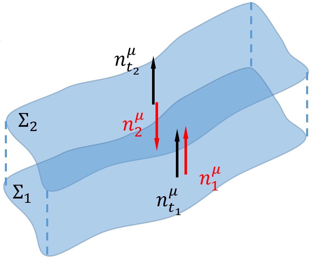
Figure 1: Disjoint hypersurfaces $\Sigma_{1}$ and $\Sigma_{2}$ over which the integration is taken. Considering these hypersurfaces are obtained by timelike slicing, then they are spacelike and their normal vectors $n_{t_{1}}^{\mu}$ and $n_{t_{2}}^{\mu}$, respectively, are timelike. For spacelike hypersurfaces, as a convention the surface normals are taken into the bulk of spacetime in the application of the Stokes’ theorem, and these surface normals are represented as $n_{1}^{\mu}$ and $n_{2}^{\mu}$ in the Figure.

A crucial point here is, as can be seen in Figure 1, $\bar{\Sigma}$ is generically not equal to $\partial\mathcal{\bar{M}}$; therefore, it can have a boundary of its own. In fact, with this definition, (17) becomes

$$Q_{\bar{\Sigma}_{2}}\left(\bar{\xi}\right)=Q_{\bar{\Sigma}_{1}}\left(\bar{\xi}\right),$$ (19)

which is a statement of charge conservation. In that case, as $\bar{\xi}_{\nu}\mathcal{E}^{\left(1\right)\mu\nu}\equiv\bar{\nabla}_{\nu}{\cal F}^{\mu\nu}\left(\bar{\xi}\right)$, where ${\cal F}^{\mu\nu}$ is an antisymmetric two-tensor, one can use the Stokes’ theorem one more time to arrive at

$$Q\left(\bar{\xi}\right)=\int_{\partial\bar{\Sigma}}d^{n-2}z\,\sqrt{\bar{\gamma}^{\left(\partial\bar{\Sigma}\right)}}\,\bar{n}_{\mu}\,\bar{\sigma}_{\nu}\,{\cal F}^{\mu\nu}\left(\bar{\xi}\right),$$ (20)

where $\bar{\sigma}_{\nu}$ is the outward unit vector on the $\left(n-2\right)$-dimensional spacelike surface $\partial\bar{\Sigma}$. Of course, the explicit form of $\mathcal{F}^{\mu\nu}\left(\bar{\xi}\right)$ can only be found from the field equations once the theory is given. For a more compact notation, one can define an anti-symmetric binormal vector

$$\bar{\epsilon}_{\mu\nu}:=\frac{1}{2}\left(\bar{n}_{\mu}\bar{\sigma}_{\nu}-\bar{n}_{\nu}\bar{\sigma}_{\mu}\right),$$ (21)

and write the charge as

$$Q\left(\bar{\xi}\right)=\int_{\partial\bar{\Sigma}}d^{n-2}z\,\sqrt{\bar{\gamma}^{\left(\partial\bar{\Sigma}\right)}}\bar{\epsilon}_{\mu\nu}{\cal F}^{\mu\nu}\left(\bar{\xi}\right).$$ (22)

It is apt now to give the explicit expressions of ${\cal F}^{\mu\nu}\left(\bar{\xi}\right)$ in the cosmological Einstein’s gravity, and in the vanishing cosmological constant case, obtain the usual expressions for the asymptotically flat spacetimes.

III.1 AD and ADM Conserved Charges

Cosmological Einstein’s gravity is defined with the action

$$I=\frac{1}{4\Omega_{n-2}G_{n}}\int d^{n}x\,\sqrt{-g}\left(R-2\Lambda\right),$$ (23)

where $G_{n}$ is $n$-dimensional Newton’s constant and $\Omega_{n-2}$ is the solid angle. The matter coupled field equations following from this action are

$$G_{\mu\nu}:=R_{\mu\nu}-\frac{1}{2}g_{\mu\nu}R+\Lambda g_{\mu\nu}=2\Omega_{n-2}G_{n}\tau_{\mu\nu}.$$ (24)

The linearization of $G_{\mu\nu}$ about its unique maximally symmetric vacuum (7) gives

$${\cal G}_{\mu\nu}^{\left(1\right)}:=R_{\mu\nu}^{\left(1\right)}-\frac{1}{2}\bar{g}_{\mu\nu}R^{\left(1\right)}-\frac{2}{n-2}\Lambda h_{\mu\nu},$$ (25)

where the linearized Ricci tensor and the scalar curvature are

$$R_{\mu\nu}^{\left(1\right)} =\frac{1}{2}\left(\bar{\nabla}_{\rho}\bar{\nabla}_{\mu}h_{\nu}^{\rho}+\bar{\nabla}_{\rho}\bar{\nabla}_{\nu}h_{\mu}^{\rho}-\bar{\Box}h_{\mu\nu}-\bar{\nabla}_{\nu}\bar{\nabla}_{\mu}h\right),$$ (26)

$$R^{\left(1\right)} =\bar{g}^{\mu\nu}R_{\mu\nu}^{\left(1\right)}-h^{\mu\nu}\bar{R}_{\mu\nu}=\bar{g}^{\mu\nu}R_{\mu\nu}^{\left(1\right)}-\frac{2}{n-2}\Lambda h.$$ (27)

In Abbott , the conserved current $\bar{\xi}_{\nu}\mathcal{G}^{\left(1\right)\mu\nu}$ was written as

$$\bar{\xi}_{\nu}{\cal G}^{\left(1\right)\mu\nu}=\bar{\nabla}_{\alpha}\left(\bar{\xi}_{\nu}\bar{\nabla}_{\beta}K^{\mu\alpha\nu\beta}-K^{\mu\beta\nu\alpha}\bar{\nabla}_{\beta}\bar{\xi}_{\nu}\right),$$ (28)

where the superpotential $K^{\mu\alpha\nu\beta}$, having the symmetries of the Riemann tensor, is

$$K^{\mu\alpha\nu\beta}:=\frac{1}{2}\left(\bar{g}^{\alpha\nu}\tilde{h}^{\mu\beta}+\bar{g}^{\mu\beta}\tilde{h}^{\alpha\nu}-\bar{g}^{\alpha\beta}\tilde{h}^{\mu\nu}-\bar{g}^{\mu\nu}\tilde{h}^{\alpha\beta}\right),\qquad\tilde{h}^{\mu\nu}:=h^{\mu\nu}-\frac{1}{2}\bar{g}^{\mu\nu}h.$$ (29)

Note that the superpotential can be compactly written by use of the Kulkarni-Nomizu product Besse of $\bar{g}$ and $\tilde{h}$ as

$$K_{\mu\alpha\nu\beta}=-\left(\bar{g}\owedge\tilde{h}\right)_{\mu\alpha\nu\beta}.$$ (30)

Therefore, one arrives at the conserved charges in cosmological Einstein’s gravity in the following compact form

$$\boxed{\phantom{\frac{\frac{\xi}{\xi}}{\frac{\xi}{\xi}}}Q\left(\bar{\xi}\right)=\frac{1}{2\Omega_{n-2}G_{n}}\int_{\partial\bar{\Sigma}}d^{n-2}z\,\sqrt{\bar{\gamma}^{\left(\partial\bar{\Sigma}\right)}}\bar{\epsilon}_{\mu\nu}\left(\bar{\xi}_{\alpha}\bar{\nabla}_{\beta}K^{\mu\nu\alpha\beta}-K^{\mu\beta\alpha\nu}\bar{\nabla}_{\beta}\bar{\xi}_{\alpha}\right),\phantom{\frac{\frac{\xi}{\xi}}{\frac{\xi}{\xi}}}}$$ (31)

which is called the Abbott-Deser charge. Here, $\bar{\epsilon}_{\mu\nu}$ is defined in (21) and other aspects of the integration are defined around equation (21). In Deser_Tekin-PRL ; Deser_Tekin-PRD , another commonly used form of (31) which suits for an extension to generic $f\left({\rm Riemann}\right)$ type theories was given as

$$Q\left(\bar{\xi}\right)=\frac{1}{4\Omega_{n-2}G_{n}}\int_{\partial\bar{\Sigma}}dS_{i}\biggl{(} \bar{\xi}_{\nu}\bar{\nabla}^{0}h^{i\nu}-\bar{\xi}_{\nu}\bar{\nabla}^{i}h^{0\nu}+\bar{\xi}^{0}\bar{\nabla}^{i}h-\bar{\xi}^{i}\bar{\nabla}^{0}h+h^{0\nu}\bar{\nabla}^{i}\bar{\xi}_{\nu}$$

$$-h^{i\nu}\bar{\nabla}^{0}\bar{\xi}_{\nu}+\bar{\xi}^{i}\bar{\nabla}_{\nu}h^{0\nu}-\bar{\xi}^{0}\bar{\nabla}_{\nu}h^{i\nu}+h\bar{\nabla}^{0}\bar{\xi}^{i}\biggr{)}.$$ (32)

Let us note a few observations before we compute the charges of some interesting spacetimes:

• There are $n\left(n+1\right)/2$ independent nontrivial conserved charges corresponding to each Killing vector of a maximally symmetric spacetime: $n$ of these result from spacetime “translations” and the $\left(n-1\right)\left(n-2\right)/2$ of these are from “rotations” summing up to $\left(n^{2}-n+2\right)/2$ conserved charges; the rest are $\left(n-1\right)$ “boosts” whose details were studied in Henneaux85 .

• The maximally symmetric spacetime which we denoted as $\bar{g}$ is assigned to have zero charges.

• $Q\left(\bar{\xi}\right)$ is invariant under the infinitesimal gauge transformations $\delta_{\zeta}h_{\mu\nu}\left(x\right)=\bar{\nabla}_{\mu}\zeta_{\nu}\left(x\right)+\bar{\nabla}_{\nu}\zeta_{\mu}\left(x\right)$ by construction since $\delta_{\zeta}\mathcal{G}_{\mu\nu}^{\left(1\right)}=0$ even though $K^{\mu\alpha\nu\beta}$ is not gauge invariant.

• We have derived (31) for $\Lambda\neq 0$, but the expression is valid for the $\Lambda=0$ case. Therefore, $Q\left(\bar{\xi}\right)$ represents the ADM charges for asymptotically flat spacetimes in generic coordinates. If one chooses the Cartesian coordinates and takes the timelike Killing vector $\xi^{\mu}=\left(-1,0,\dots,0\right)$, then (31) reduces to the celebrated ADM mass

  $$M_{{\rm ADM}}=\frac{1}{2\Omega_{n-2}G_{n}}\int_{S^{n-2}} dS_{i} \left(\partial_{j}h^{ij}-\partial^{i}h_{jj}\right),$$ (33)

  where the integral is to be evaluated on a sphere at spatial infinity. Similarly, angular momentum (or momenta) has a similar expression

  $$J=\frac{1}{2\Omega_{n-2}G_{n}}\int_{S^{n-2}} dS_{i} \left(\bar{\xi}^{i}\partial_{j}h^{0j}-\bar{\xi}_{j}\partial^{i}h^{0j}\right),$$ (34)

  where $\bar{\xi}^{i}$ is the corresponding Killing vector. In practice, to compute the conserved charges of a given solution, using the coordinate independent expression (31) is much more efficient, especially if the metric is complicated.

• Even if one takes the background spacetime to be nonmaximally symmetric, but with at least one Killing vector field, one arrives at the same charge expression (31). This is a highly nontrivial point and not immediately clear, but one can run the same computation as above without the assumption of maximal symmetry and observe that one has additional parts

  $$\bar{\xi}_{\nu}{\cal G}_{L}^{\mu\nu}= \bar{\nabla}_{\alpha}\left(\bar{\xi}_{\nu}\bar{\nabla}_{\beta}K^{\mu\alpha\nu\beta}-K^{\mu\beta\nu\alpha}\bar{\nabla}_{\beta}\bar{\xi}_{\nu}\right)$$

  $$+\bar{\xi}_{\nu}h^{\mu\alpha}\bar{G}_{\alpha}^{\phantom{\alpha}\nu}+\frac{1}{2}\bar{\xi}^{\mu}h^{\rho\sigma}\bar{G}_{\rho\sigma}-\frac{1}{2}\bar{\xi}_{\rho}\bar{G}^{\mu\rho}h,$$ (35)

  but once the background field equations are used, the additional parts drop out. Hence, the earlier result derived for the maximally symmetric vacuum is valid for all Einstein spaces with a Killing vector field Bouchareb ; Nazaroglu ; Devecioglu . To see this result explicitly, let us lay out the details of the computation since it will be relevant for theories that extend Einstein’s theory and have nonmaximally symmetric vacua (for example, in three dimensions topologically massive gravity is an example). For a nonmaximally symmetric background $\bar{g}_{\mu\nu}$, the linearized Einstein tensor have the form

  $${\cal G}_{\mu\nu}^{\left(1\right)}=R_{\mu\nu}^{\left(1\right)}-\frac{1}{2}\bar{g}_{\mu\nu}R_{\left(1\right)}+\Lambda h_{\mu\nu}-\frac{1}{2}h_{\mu\nu}\bar{R},$$ (36)

  with the help of (26) and the first equality of (27), ${\cal G}_{\mu\nu}^{\left(1\right)}$ reduces to

  $${\cal G}_{\mu\nu}^{\left(1\right)}= \frac{1}{2}\left(\bar{\nabla}_{\rho}\bar{\nabla}_{\mu}h_{\nu}^{\rho}+\bar{\nabla}_{\rho}\bar{\nabla}_{\nu}h_{\mu}^{\rho}-\bar{\Box}h_{\mu\nu}-\bar{\nabla}_{\nu}\bar{\nabla}_{\mu}h\right)$$

  $$-\frac{1}{2}\bar{g}_{\mu\nu}\left(\bar{\nabla}_{\rho}\bar{\nabla}_{\sigma}h^{\rho\sigma}-\bar{\Box}h-h^{\rho\sigma}\bar{R}_{\rho\sigma}\right)+\Lambda h_{\mu\nu}-\frac{1}{2}h_{\mu\nu}\bar{R}.$$ (37)

  We assume that the background has at least one Killing vector field. In trying to find a form as $\bar{\xi}_{\nu}{\cal G}^{\left(1\right)\mu\nu}=\bar{\nabla}_{\nu}\mathcal{F}^{\mu\nu}$ where $\mathcal{F}^{\mu\nu}$ is antisymmetric, following Abbott it is better to write $\bar{\xi}_{\nu}{\cal G}^{\left(1\right)\mu\nu}$ as $\bar{\xi}_{\nu}{\cal G}^{\left(1\right)\mu\nu}\sim\bar{\nabla}_{\alpha}\bar{\nabla}_{\beta}K^{\alpha\beta\mu\nu}+X^{\mu\nu}$ since one just needs to handle an interchange of order in derivatives for the term $\bar{\xi}_{\nu}{\cal G}^{\left(1\right)\mu\nu}\sim\bar{\xi}_{\nu}\bar{\nabla}_{\alpha}\bar{\nabla}_{\beta}K^{\alpha\beta\mu\nu}+\bar{\xi}_{\nu}X^{\mu\nu}$ as

  $$\bar{\xi}_{\nu}{\cal G}^{\left(1\right)\mu\nu}\sim\bar{\xi}_{\nu}\bar{\nabla}_{\alpha}\bar{\nabla}_{\beta}K^{\alpha\beta\mu\nu}+\bar{\xi}_{\nu}X^{\mu\nu}=\bar{\nabla}_{\alpha}\left(\bar{\xi}_{\nu}\bar{\nabla}_{\beta}K^{\alpha\beta\mu\nu}\right)-\left(\bar{\nabla}_{\alpha}\bar{\xi}_{\nu}\right)\bar{\nabla}_{\beta}K^{\alpha\beta\mu\nu}+\bar{\xi}_{\nu}X^{\mu\nu}.$$ (38)

  To work out what $K^{\alpha\beta\mu\nu}$ and $X^{\mu\nu}$ are for the Einstein’s theory, ${\cal G}_{L}^{\mu\nu}$ can be rewritten as the derivative terms plus nonderivative terms:

  $${\cal G}_{L}^{\mu\nu}= \frac{1}{2}\bar{\nabla}_{\alpha}\bar{\nabla}_{\beta}\left(\bar{g}^{\nu\beta}h^{\mu\alpha}+\bar{g}^{\mu\beta}h^{\alpha\nu}-\bar{g}^{\alpha\beta}h^{\mu\nu}-\bar{g}^{\mu\nu}h^{\alpha\beta}+\bar{g}^{\mu\nu}\bar{g}^{\alpha\beta}h-\bar{g}^{\mu\alpha}\bar{g}^{\nu\beta}h\right)$$

  $$+\frac{1}{2}\bar{g}^{\mu\nu}h^{\rho\sigma}\bar{R}_{\rho\sigma}+\Lambda h_{\mu\nu}-\frac{1}{2}h_{\mu\nu}\bar{R}.$$ (39)

  From the first line, we want to define the $K$ tensor such that it has the same symmetries as the Riemann tensor. Comparing with the maximally symmetric Riemann tensor $\bar{R}_{\mu\alpha\nu\beta}\sim\Lambda\left(\bar{g}_{\mu\nu}\bar{g}_{\alpha\beta}-\bar{g}_{\mu\beta}\bar{g}_{\alpha\nu}\right),$ one can see that except the first and the last terms, the others combine to define the desired $K^{\mu\alpha\nu\beta}$. Order change for the last term is automatic, and once we have the order change in the first term, ${\cal G}_{L}^{\mu\nu}$ becomes

  $${\cal G}_{L}^{\mu\nu}=\bar{\nabla}_{\alpha}\bar{\nabla}_{\beta}K^{\mu\alpha\nu\beta}+X^{\mu\nu},$$

  where

  $$K^{\mu\alpha\nu\beta}\equiv\frac{1}{2}\left(\bar{g}^{\alpha\nu}\tilde{h}^{\mu\beta}+\bar{g}^{\mu\beta}\tilde{h}^{\alpha\nu}-\bar{g}^{\alpha\beta}\tilde{h}^{\mu\nu}-\bar{g}^{\mu\nu}\tilde{h}^{\alpha\beta}\right),\qquad\tilde{h}^{\mu\nu}\equiv h^{\mu\nu}-\frac{1}{2}\bar{g}^{\mu\nu}h,$$ (40)

  and the “fudge” tensor reads

  $$X^{\mu\nu} \equiv\frac{1}{2}\bar{g}^{\nu\beta}\left[\bar{\nabla}_{\alpha},\bar{\nabla}_{\beta}\right]h^{\mu\alpha}+\frac{1}{2}\bar{g}^{\mu\nu}h^{\rho\sigma}\bar{R}_{\rho\sigma}+\Lambda h_{\mu\nu}-\frac{1}{2}h_{\mu\nu}\bar{R}$$

  $$=\frac{1}{2}\left(h^{\mu\alpha}\bar{R}_{\alpha}^{\phantom{\alpha}\nu}-\bar{R}^{\mu\alpha\nu\beta}h_{\alpha\beta}\right)+\frac{1}{2}\bar{g}^{\mu\nu}h^{\rho\sigma}\bar{R}_{\rho\sigma}+\Lambda h^{\mu\nu}-\frac{1}{2}h^{\mu\nu}\bar{R}.$$

  Note that both $\bar{\nabla}_{\alpha}\bar{\nabla}_{\beta}K^{\mu\alpha\nu\beta}$ and $X^{\mu\nu}$ are not symmetric in $\mu$ and $\nu$. Now, let us find the antisymmetric tensor $\mathcal{F}^{\mu\nu}$ by rearranging $\bar{\xi}_{\nu}{\cal G}_{L}^{\mu\nu}$ with the help of the identity $\bar{\nabla}_{\beta}\bar{\nabla}_{\alpha}\bar{\xi}_{\nu}=\bar{R}_{\phantom{\rho}\beta\alpha\nu}^{\rho}\bar{\xi}_{\rho}$ as

  $$\bar{\xi}_{\nu}{\cal G}_{L}^{\mu\nu}=\bar{\nabla}_{\alpha}\left(\bar{\xi}_{\nu}\bar{\nabla}_{\beta}K^{\mu\alpha\nu\beta}-K^{\mu\beta\nu\alpha}\bar{\nabla}_{\beta}\bar{\xi}_{\nu}\right)+K^{\mu\alpha\nu\beta}\bar{R}_{\phantom{\rho}\beta\alpha\nu}^{\rho}\bar{\xi}_{\rho}+X^{\mu\nu}\bar{\xi}_{\nu},$$ (41)

  where the first term is in the desired form. Note that $K^{\mu\alpha\nu\beta}\bar{R}_{\phantom{\rho}\beta\alpha\nu}^{\rho}$ can also be written as $K^{\mu\alpha\nu\beta}\bar{R}_{\phantom{\rho}\alpha\beta\nu}^{\rho}/2$. Using the background cosmological Einstein tensor

  $$\bar{G}_{\mu\nu}=\bar{R}_{\mu\nu}-\frac{1}{2}\bar{g}_{\mu\nu}\bar{R}+\Lambda\bar{g}_{\mu\nu},$$ (42)

  we can recast $\bar{\xi}_{\nu}{\cal G}_{L}^{\mu\nu}$ to (35). As a summary, all of this says that the AD conserved charges (31) or (32) are valid for all Einstein spaces with at least one Killing vector field.

III.2 Large diffeomorphisms (gauge transformations)

In the above construction of the conserved charges, we noted that the results are invariant under small diffeomorphisms that act on $h_{\mu\nu}$ as $\delta_{\zeta}h_{\mu\nu}\left(x\right)=\bar{\nabla}_{\mu}\zeta_{\nu}\left(x\right)+\bar{\nabla}_{\nu}\zeta_{\mu}\left(x\right)$ which is valid as long as $\left|\bar{\nabla}_{\mu}\zeta_{\nu}\left(x\right)\right|\ll\left|h_{\mu\nu}\left(x\right)\right|$ is satisfied in the given coordinate system for the given chart. Here, we briefly address the case of large diffeomorphisms and show how they split the charges assigned to a given geometry into various sectors. For the sake of simplicity, we discuss the Minkowski spacetime and follow the arguments in ST which was based on DenisovSolovev ; BrayChrusciel . In spherical coordinates, the four-dimensional flat Minkowski spacetime has the metric

$${\rm d}s^{2}=-{\rm d}t^{2}+{\rm d}r^{2}+r^{2}{\rm d}\Omega,\qquad{\rm d}\Omega:={\rm d}\theta^{2}+\sin^{2}\theta{\rm d}\phi^{2}$$ (43)

Needless to say, any coordinate change will keep the Riemann tensor of this spacetime to be zero. Consider the following specific coordinate transformations

$$t=f\left(\tau,\rho\right),\qquad r=k\left(\tau,\rho\right),$$

and $\theta$, $\phi$ are kept intact. Then, the metric in these new coordinates $\left(\tau,\rho,\theta,\phi\right)$ reads

$${\rm d}s^{2}=\left(\dot{k}^{2}-\dot{f}^{2}\right)\,{\rm d}\tau^{2}+2\left(\dot{k}k^{\prime}-\dot{f}f^{\prime}\right)\,{\rm d}\tau{\rm d}\rho+\left(k^{\prime}{}^{2}-f^{\prime}{}^{2}\right)\,{\rm d}\rho^{2}+k^{2}{\rm d}\Omega,$$ (44)

where we have suppressed the arguments of the functions, and defined $\dot{f}:=\partial f/\partial\tau$ and $f^{\prime}:=\partial f/\partial\rho$. Taking (43) as the background geometry with zero mass, we can calculate the mass of (44) with respect to the background. More properly, we can identify the background metric from (44) as $f=\tau$ and $k=\rho$. Then, the deviation from the background reads

$$h_{\mu\nu}dx^{\mu}dx^{\nu}=\left(1+\dot{k}^{2}-\dot{f}^{2}\right)\,{\rm d}\tau^{2}+2\left(\dot{k}k^{\prime}-\dot{f}f^{\prime}\right)\,{\rm d}\tau{\rm d}\rho+\left(-1+k^{\prime}{}^{2}-f^{\prime}{}^{2}\right)\,{\rm d}\rho^{2}+\left(-\rho^{2}+k^{2}\right){\rm d}\Omega.$$ (45)

Using (33) and taking the background Killing vector as $\bar{\xi}^{\mu}=\left(-1,0,0,0\right)$, the ADM mass-energy of (44) becomes

$$E=\left.\frac{1}{2G\rho}\left(-\rho^{2}\left(f^{\prime}\right)^{2}+\left(k-\rho k^{\prime}\right)^{2}\right)\right|_{\rho\rightarrow\infty}.$$ (46)

It is clear that $M$ can take any value depending on the choices of the functions $f$ and $k$. Let us consider a specific example with

$$f\left(\tau,\rho\right)=\tau,\qquad\qquad k\left(\tau,\rho\right)=\rho y\left(\tau\right)+2\sqrt{2Gm\rho},$$ (47)

where $y$ is an arbitrary function of $\tau$ and $m$ is a positive constant. For this choice $M=m$. More generally, for

$$k\left(\tau,\rho\right)=\rho y\left(\tau\right)+\left(Gm\rho\right)^{1-s},$$ (48)

$E$ diverges for $s<1/2$ and vanishes for $s>1/2$. Even negative values for the total mass is possible. For example, choosing

$$k\left(\tau,\rho\right)=\rho,\qquad\qquad f\left(\tau,\rho\right)=y\left(\tau\right)+2\sqrt{2Gm\rho},$$ (49)

yields a negative mass of $E=-m$.

Without much ado, let us give a similar example for the case of angular momentum: Let us consider the following coordinate transformations

$$r=k\left(t,\rho\right)=\rho\sqrt{mt}+\sqrt{Gm\rho},\qquad\phi=p\left(\rho,\psi\right)=\psi+Gm^{3}a\left(m\rho\right)^{s},$$ (50)

where $a$ is a parameter with dimension of length. Note that we kept $t$, $\theta$ intact. Then, the metric in these new coordinates read

$${\rm d}s^{2}= -\left(1-\frac{m\rho^{2}}{4t}\right)\text{d$t$}^{2}+\left(1+\frac{1}{2}\sqrt{\frac{G}{t\rho}}\right)m\rho\text{d$\rho$}\text{d$t$}$$

$$+\left(m^{2}a^{2}s^{2}\sin^{2}\theta\left(1+\sqrt{\frac{G}{t\rho}}\right)^{2}\left(m\rho\right)^{2s}+\left(1+\frac{1}{2}\sqrt{\frac{G}{t\rho}}\right)^{2}\right)m\,t\text{d$\rho$}^{2}$$

$$+2m\,a\,s\sin^{2}\theta\left(1+\sqrt{\frac{G}{t\rho}}\right)^{2}\left(m\rho\right)^{s+1}t\text{d$\rho$}\text{d$\psi$}+\left(1+\sqrt{\frac{G}{t\rho}}\right)^{2}m\rho^{2}t{\rm d}\Omega,$$ (51)

which is diffeomorphic to the Minkowski spacetime and of course it is Riemann flat. Using the conserved charge expression (31), for the Killing vector fields $\bar{\xi}^{\mu}=\left(-1,0,0,0\right)$ and $\bar{\xi}^{\mu}=\left(0,0,0,1\right)$, one finds

$$E=\frac{m}{4}+\frac{2}{3}a^{2}m^{6}s^{2}\left(m\rho\right)^{2s+1}t,\qquad J=-\frac{m\,a\,s\left(m\rho\right)^{s+3}}{3},$$ (52)

which must be evaluated in the limit $\rho\rightarrow\infty$. Both of the terms become finite for $s=-3$ which yields

$$E=\frac{m}{4},\qquad J=m\,a.$$ (53)

All these arguments show that the flat Minkowski spacetime has infinitely many diffeomorphic copies that all have vanishing Riemann tensor but with different ADM energies and angular momenta. In the light of this discussion, the conventional positive energy theorem that assigns zero energy, and linear and angular momenta to the flat Minkowski spacetime Schoen ; Witten ; Deser ; Grisaru ; Parker ; Nester also assumes that the metric components in the example discussed above decay sufficiently fast at infinity, that is the $s>1/2$ case with vanishing energy.

III.3 Schwarzschild-(A)dS Black Holes in $n$-dimensions

Let us apply the AD construction to the immediate natural setting of the static spherically symmetric black hole in (A)dS. The metric in static coordinates reads

$${\rm d}s^{2}=-\left(1-\left(\frac{r_{0}}{r}\right)^{n-3}+\frac{r^{2}}{\ell^{2}}\right){\rm d}t^{2}+\left(1-\left(\frac{r_{0}}{r}\right)^{n-3}+\frac{r^{2}}{\ell^{2}}\right)^{-1}{\rm d}r^{2}+r^{2}{\rm d}\Omega_{n-2}^{2},$$ (54)

where $\ell^{2}:=-\frac{(n-2)(n-1)}{2\Lambda}$ and $n>3$. The background metric corresponds to $r_{0}=0$ with the timelike Killing vector $\xi^{\mu}=\left(-1,\vec{0}\right)$ satisfying $\bar{g}_{\mu\nu}\bar{\xi}^{\mu}\bar{\xi}^{\nu}=-\left(1+\frac{r^{2}}{\ell^{2}}\right)$. [Formally, we can carry out the same construction for the de Sitter case with $\ell\rightarrow i\ell$, but clearly due to the cosmological horizon at a finite $r$ coordinate, $\bar{\xi}^{\mu}$ fails to be timelike everywhere, and hence a global time does not exist. Therefore, for black holes in dS only small black hole limit can be approximately considered, for more on this see Deser_Tekin-PRD .] For the case of AdS background, the result of the energy computation based on (31) turns out to be as expected

$$E=\frac{n-2}{4G_{n}}r_{0}^{n-3},$$ (55)

and in four dimensions $r_{0}=2Gm$, and $E=M$ as expected.

III.4 Kerr-AdS Black Holes in $n$-dimensions

Let us now consider a more complicated example by adding rotations to the $n$-dimensional black hole. The metric was given in Gibbons in the Kerr-Schild form KerrSchild ; GursesGursey as

$${\rm d}s^{2}={\rm d}\bar{s}^{2}+\frac{2mG_{n}}{U}\left(k_{\mu}{\rm d}x^{\mu}\right)^{2},$$ (56)

where $m$ is a real parameter, $k_{\mu}{\rm d}x^{\mu}$ is a one-form defined below, $U$ is a function of the coordinate $r$ and the direction cosines $\mu_{i}$s as

$$U:=r^{\epsilon}\sum_{i=1}^{N+\epsilon}\frac{\mu_{i}^{2}}{r^{2}+a_{i}^{2}}\prod_{j=1}^{N}\left(r^{2}+a_{j}^{2}\right),\qquad\sum_{i=1}^{N+\epsilon}\mu_{i}^{2}=1,$$ (57)

with $\epsilon=0/1$ for odd/even dimensions and $n=2N+1+\epsilon$. Here, $N$ refers to the number of rotation parameters $a_{i}$ associated to the azimuthal angles $\phi_{i}$s. For even $n$, one should note that $a_{N+1}=0$ since $\phi_{N+1}$ does not exist. The background metric reads

$${\rm d}\bar{s}^{2}= -W\left(1+\frac{r^{2}}{\ell^{2}}\right){\rm d}t^{2}+F{\rm d}r^{2}+\sum_{i=1}^{N+\epsilon}\frac{r^{2}+a_{i}^{2}}{1-\frac{a_{i}^{2}}{\ell^{2}}}{\rm d}\mu_{i}^{2}+\sum_{i=1}^{N}\frac{r^{2}+a_{i}^{2}}{1-\frac{a_{i}^{2}}{\ell^{2}}}\mu_{i}^{2}{\rm d}\phi_{i}^{2}$$

$$-\frac{1}{W\ell^{2}\left(1+\frac{r^{2}}{\ell^{2}}\right)}\left(\sum_{i=1}^{N+\epsilon}\frac{\left(r^{2}+a_{i}^{2}\right)\mu_{i}{\rm d}\mu_{i}}{1-\frac{a_{i}^{2}}{\ell^{2}}}\right)^{2},$$ (58)

where again $W$ and $F$ are functions of the coordinates $r$ and $\mu_{i}$s as

$$W:=\sum_{i=1}^{N+\epsilon}\frac{\mu_{i}^{2}}{1-\frac{a_{i}^{2}}{\ell^{2}}},\qquad\qquad\qquad F:=\frac{1}{1+\frac{r^{2}}{\ell^{2}}}\sum_{i=1}^{N+\epsilon}\frac{r^{2}\mu_{i}^{2}}{r^{2}+a_{i}^{2}}.$$ (59)

The one-form $k_{\mu}{\rm d}x^{\mu}$ is given as

$$k_{\mu}{\rm d}x^{\mu}=F{\rm d}r+W{\rm d}t-\sum_{i=1}^{N}\frac{a_{i}\mu_{i}^{2}}{1-\frac{a_{i}^{2}}{\ell^{2}}}{\rm d}\phi_{i},$$ (60)

which is null and geodesic for both the background and the full metrics which conveys the spirit of the Kerr-Schild construction. The $\ell\rightarrow\infty$ limit of (56) yields the Myers-Perry black hole MyersPerry and $a_{i}\rightarrow 0$ yields the Schwarzschild-Tangherlini black holes. Defining the perturbation as

$$h_{\mu\nu}=\frac{2mG_{n}}{U}k_{\mu}k_{\nu},$$ (61)

which yields $h=0$. Note that the Kerr-Schild form is quite convenient for perturbative calculations as the perturbation $h_{\mu\nu}$ is exact.

We can now run the machinery and calculate the energy and angular momenta of these solutions (56). For the energy, we shall take $\bar{\xi}^{\mu}=(-1,\vec{0})$, and then the energy integral becomes

$$E=\frac{1}{4\Omega_{n-2}G_{n}}\int_{\partial\bar{\Sigma}}dS_{r}\left(\bar{g}_{00}\bar{\nabla}^{0}h^{r0}+\bar{g}_{00}\bar{\nabla}^{r}h^{00}+h^{0\nu}\bar{\nabla}^{r}\bar{\xi}_{\nu}-h^{r\nu}\bar{\nabla}^{0}\bar{\xi}_{\nu}+\bar{\nabla}_{\nu}h^{r\nu}\right),$$

and expanding the covariant derivatives, one arrives at

$$E=\frac{1}{4\Omega_{n-2}G_{n}}\int_{\partial\bar{\Sigma}}d\Omega_{n-2}\sqrt{\left|\bar{g}\right|}\Biggl{(} \bar{g}_{00}\bar{g}^{rr}\partial_{r}h^{00}+\frac{1}{2}h^{00}\bar{g}^{rr}\partial_{r}\bar{g}_{00}-\frac{m}{U}\bar{g}^{00}\partial_{r}\bar{g}_{00}+2m\partial_{r}U^{-1}$$

$$+\frac{2m}{U}\bar{g}^{rr}\partial_{r}\bar{g}_{rr}-\frac{m}{U}g^{rr}k^{i}k^{j}\partial_{r}\bar{g}_{ij}+\frac{m}{U}\bar{g}^{ij}\partial_{r}\bar{g}_{ij}\Biggr{)}.$$ (62)

The integral is to be computed on the boundary $\partial\bar{\Sigma}$ which is located at $r\rightarrow\infty$. The integration, whose details can be found in Kanik ; Tekin_et_al , yields the energy of the $n$-dimensional rotating black hole as

$$E_{n}=\frac{m}{\Xi}\sum_{i=1}^{N}\left(\frac{1}{\Xi_{i}}-\frac{1}{2}\left(1-\epsilon\right)\right).$$ (63)

where we have defined

$$\Xi\equiv\prod_{i=1}^{N}\left(1-\frac{a_{i}^{2}}{\ell^{2}}\right),\qquad\Xi_{i}\equiv 1-\frac{a_{i}^{2}}{\ell^{2}}.$$ (64)

In four dimensions, one gets a modified energy expression due to the rotation

$$E=\frac{m}{\left(1-\frac{a^{2}}{\ell^{2}}\right)^{2}}.$$ (65)

which in the $\ell\rightarrow\infty$ limit or $a\rightarrow 0$ limit yields the expected result. Note that $a\neq\ell$ for the metric to be nonsingular. In addition, this result agrees (up to a constant factor) with those of Pope ; Deruelle .

Similarly, taking the Killing vector $\xi_{(i)}^{\mu}=\left(0,...,0,1_{i},0,..\right)$ corresponding to the $i^{\mbox{th}}$ azimuthal angle $\phi_{i}$ out of $N$ possibilities, one finds the corresponding Killing charge to be

$$Q_{i}= \frac{1}{4\Omega_{n-2}G_{n}}\int_{\partial\bar{\Sigma}}dS_{r}\left(\bar{g}_{\phi_{i}\phi_{i}}\bar{\nabla}^{0}h^{r\phi_{i}}-\bar{g}_{\phi_{i}\phi_{i}}\bar{\nabla}^{r}h^{0\phi_{i}}+h^{0\nu}\bar{\nabla}^{r}\bar{\xi}_{\nu}-h^{r\nu}\bar{\nabla}^{0}\bar{\xi}_{\nu}\right)$$

$$= \frac{1}{4\Omega_{n-2}G_{n}}\int_{\partial\bar{\Sigma}}d\Omega_{n-2}\sqrt{\left|\bar{g}\right|}\left(-\bar{g}_{\phi_{i}\phi_{i}}\bar{g}^{rr}\bar{g}^{00}\partial_{r}h_{0}^{\;\phi_{i}}\right).$$ (66)

which yields Kanik ; Tekin_et_al

$$J_{i}=\frac{ma_{i}}{\Xi\Xi_{i}},$$ (67)

in agreement with Pope ; Deruelle . We can relate the total energy and angular momenta as

$$E=\sum_{i=1}^{N}\frac{J_{i}}{a_{i}},$$ (68)

for even dimensions and for the odd case, one has

$$E=\sum_{i=1}^{N}\frac{J_{i}}{a_{i}}-\frac{Nm}{2\Xi},$$ (69)

where there is an additional piece independent of the angular momenta, but for any $J_{i}\rightarrow 0$, one must take the limit $J_{i}/a_{i}\rightarrow m$.

III.5 Computation of the charges for the solitons

We can use the AD formalism to compute the conserved charges of solitonic (nonsingular) solutions of gravity theories. These are quite interesting objects for various reasons; one of them being their possible negative but bounded mass. Here, we follow Cebeci .

III.5.1 The $AdS$ Soliton

Horowitz and Myers Horowitz analytically continued the near extremal $p$-brane solutions to obtain the following metric the so-called “AdS Soliton";

$$ds^{2}=\frac{r^{2}}{\ell^{2}}\left[\left(1-\frac{r_{0}^{p+1}}{r^{p+1}}\right){\rm d}\tau^{2}+\sum_{i=1}^{p-1}\left({\rm d}x^{i}\right)^{2}-{\rm d}t^{2}\right]+\left(1-\frac{r_{0}^{p+1}}{r^{p+1}}\right)^{-1}\,\frac{\ell^{2}}{r^{2}}\,{\rm d}r^{2}, \left(r\geq r_{0}\right)$$ (70)

The coordinates on the $p$-brane are $t$ and $x^{i}$ ($i=1,...,p-1$). The conical singularity at $r=r_{0}$ is removed if $\tau$ has a period $\beta=4\pi\ell^{2}/(r_{0}(p+1))$. Using the Killing vector $\bar{\xi}^{\mu}=(-1,0,...,0)$ in (31) and taking the background to be $r_{0}=0$, one arrives at the energy density of the solitonic brane $E/V_{n-3}$ as

$$\frac{E}{V_{n-3}}=-\frac{\pi}{(n-1)\,\Omega_{n-2}\,G_{n}}\,\frac{r_{0}^{n-2}}{\ell^{n-2}}\,,$$ (71)

which matches the result of Horowitz computed with the energy definition of Hawking-Horowitz HawkingHorowitz up to trivial normalization factors.

III.5.2 Eguchi-Hanson Solitons

In odd dimensional cosmological spacetimes, Clarkson and Mann clarkson found solitonic solutions that are called Eguchi-Hanson solitons since they are analogs to the even dimensional Eguchi-Hanson metrics eguchi which approach asymptotically to $AdS/Z_{p}$, where $p\geq 3$, instead of the global AdS spacetime. These solitons have lower energy than the global AdS spacetime as was demonstrated by Clarkson and Mann with the boundary counter-term method of henningson ; 97 for the case of five dimensions. This method requires each dimension to be worked out separately as the counter-terms vary when the dimension changes. But, the AD method can be applied for a generic dimensional solution. The Eguchi-Hanson soliton metric is

$$ds^{2} = -g\,{\rm d}t^{2}+\left(\frac{2r}{n-1}\right)^{2}\,f\,\left[{\rm d}\psi+\sum_{i=1}^{(n-3)/2}\cos\theta_{i}\,{\rm d}\phi_{i}\right]^{2}$$ (72)

$$+\frac{dr^{2}}{g\,f}+\frac{r^{2}}{n-1}\,\sum_{i=1}^{(n-3)/2}\,\left({\rm d}\theta_{i}^{2}+\sin^{2}\theta_{i}\,{\rm d}\phi_{i}^{2}\right)\,,$$

where

$$g(r)=1\mp\frac{r^{2}}{\ell^{2}}\;\;,\quad f(r)=1-\left(\frac{r_{0}}{r}\right)^{n-1}\,.$$ (73)

The solution exists both in dS and AdS; but, let us concentrate in the AdS case and to remove the string-like singularity at $r=r_{0}$, $\psi$ must have a period $4\pi/p$ and the constant $r_{0}$ is given as

$$r_{0}^{2}=\ell^{2}\,(\frac{p^{2}}{4}-1)\,.$$ (74)

Taking the background to be $r_{0}=0$, the energy for $\bar{\xi}^{\mu}=(-1,0,...,0)$ is

$$E=-\frac{(4\pi)^{(n-1)/2}\,r_{0}^{n-1}}{p\,\ell^{2}\,(n-1)^{(n-1)/2}\,\Omega_{n-2}\,G_{n}}\,,$$ (75)

which reduces to

$$E=-\frac{r_{0}^{4}}{4\,p\,\ell^{2}\,G_{5}}\,,$$ (76)

for $n=5$. In the counter-term method, the global AdS has a finite energy whereas in our method it has zero energy by definition. Once that is taken into account, both methods give the same result up to a trivial normalization factor.

III.6 Energy of the Taub-NUT-Reissner-Nordstr$\ddot{\text{o}}$m metric

As some other nontrivial applications of the AD formalism for spacetimes with nontrivial topology, let us consider the four and six dimensional Taub-NUT-Reissner-Nordstr$\ddot{\text{o}}$m solutions stelea1 . For $n=4$, the metric is

$$ds^{2}=-f\,\Bigl{(}{\rm d}t-2\,N\,\cos\theta\,{\rm d}\phi\Bigr{)}^{2}+\frac{{\rm d}r^{2}}{f}+\left(r^{2}+N^{2}\right)\,\left({\rm d}\theta^{2}+\sin^{2}\theta\,{\rm d}\phi^{2}\right)\,,$$ (77)

where $N$ is the nut charge and

$$f(r)=\frac{r^{4}+(\ell^{2}+6N^{2})\,r^{2}-2\,m\,\ell^{2}\,r-3N^{4}+\ell^{2}\,(q^{2}-N^{2})}{\ell^{2}\,(r^{2}+N^{2})}\,.$$ (78)

The naive identification of the background as $m=q=N=0$ yields a divergent energy for any nonzero $N$ and $m$ configuration. This is because $N=0$ and $N\neq 0$ spacetimes are not in the same topological class; hence, for a meaningful use of the formalism one should work within a fixed $N$ sector and choose the background to be $m=q=0$; but, keep $N$ finite. This yields for (77)

$$E=\frac{m}{G_{4}}\,,$$ (79)

again for the timelike Killing vector $\bar{\xi}=(-1,0,0,0)$. In $n=6$, the metric reads

$$ds^{2} = -f\,\Bigl{(}{\rm d}t-2\,N\,\cos\theta_{1}\,{\rm d}\phi_{1}-2\,N\,\cos\theta_{2}\,{\rm d}\phi_{2}\Bigr{)}^{2}+\frac{{\rm d}r^{2}}{f}$$ (80)

$$+\left(r^{2}+N^{2}\right)\,\left(d\theta_{1}^{2}+\sin^{2}\theta_{1}\,{\rm d}\phi_{1}^{2}+{\rm d}\theta_{2}^{2}+\sin^{2}\theta_{2}\,{\rm d}\phi_{2}^{2}\right)\,,$$

where the metric function $f$ is

$$f(r) = \frac{q^{2}\,\left(3r^{2}+N^{2}\right)}{\left(r^{2}+N^{2}\right)^{4}}$$

$$+\frac{1}{3\ell^{2}\left(r^{2}+N^{2}\right)^{2}}\left(\ell^{2}\left(-3N^{4}-6mr+6N^{2}r^{2}+r^{4}\right)-15N^{6}+45N^{4}r^{2}+15N^{2}r^{4}+3r^{6}\right).$$

Similarly, choosing the background to be $m=q=0$ but $N\neq 0$, and the energy can be computed as

$$E=12\,\frac{m}{G_{6}}\,.$$ (81)

Next we turn our attention to generic gravity theories with more powers of curvature.

IV Charges of Quadratic Curvature Gravity

We will work out the construction of conserved charges for generic gravity theories with an action of the form

$$I=\int d^{D}x\,\sqrt{-\left|g\right|}\,f\left(R_{\rho\sigma}^{\mu\nu}\right),$$ (82)

where $F$ is a smooth function of the Riemann tensor and its contractions given in the form $R_{\rho\sigma}^{\mu\nu}:=R_{\phantom{\mu\nu}\rho\sigma}^{\mu\nu}$, and hence contractions do not require the metric. For example, $R_{\phantom{\nu}\sigma}^{\nu}=R_{\mu\sigma}^{\mu\nu}$ and $R=R_{\mu\nu}^{\mu\nu}$. Here, we start with the quadratic theory

$$I=\int d^{n}x\sqrt{-g}\left(\frac{1}{\kappa}\left(R-2\Lambda_{0}\right)+\alpha R^{2}+\beta R_{\mu\nu}R^{\mu\nu}+\gamma\left(R_{\mu\nu\rho\sigma}R^{\mu\nu\rho\sigma}-4R_{\mu\nu}R^{\mu\nu}+R^{2}\right)\right),$$ (83)

whose results can be easily extended to the above more general action as we shall lay out in more detail. We have organized the last part into the Gauss-Bonnet combination which does not contribute to the field equations for $n\leq 4$ (in fact, it vanishes identically in $n\leq 3$ and becomes a surface term for $n=4$). Arguments from string theory require $\alpha$ and $\beta$ to vanish Zwiebach , or in general using field redefinitions in a generic theory which is not truncated at the quadratic order as (83), one can get rid off the $\alpha$ and $\beta$ terms. But, here our goal is to consider (83) to be exact (with all its deficiencies such as having a ghost for nonzero $\beta$) and construct the conserved charges. For this purpose, we need the field equations which read

$$\frac{1}{\kappa}\left(R_{\mu\nu}-\frac{1}{2}g_{\mu\nu}R+g_{\mu\nu}\Lambda_{0}\right)+2\alpha R\left(R_{\mu\nu}-\frac{1}{4}g_{\mu\nu}R\right)+\left(2\alpha+\beta\right)\left(g_{\mu\nu}\Box-\nabla_{\mu}\nabla_{\nu}\right)R$$

$$+2\gamma\left(RR_{\mu\nu}-2R_{\mu\sigma\nu\rho}R^{\sigma\rho}+R_{\mu\sigma\rho\tau}R_{\nu}^{\phantom{\nu}\sigma\rho\tau}-2R_{\mu\sigma}R_{\phantom{\sigma}\nu}^{\sigma}-\frac{1}{4}g_{\mu\nu}\left(R_{\alpha\beta\rho\sigma}R^{\alpha\beta\rho\sigma}-4R_{\alpha\beta}R^{\alpha\beta}+R^{2}\right)\right)$$

$$+\beta\Box\left(R_{\mu\nu}-\frac{1}{2}g_{\mu\nu}R\right)+2\beta\left(R_{\mu\sigma\nu\rho}-\frac{1}{4}g_{\mu\nu}R_{\sigma\rho}\right)R^{\sigma\rho} =\tau_{\mu\nu}.$$ (84)

In general, there are two maximally symmetric vacua whose effective cosmological constant $\Lambda$ is determined by the quadratic equation

$$\frac{\Lambda-\Lambda_{0}}{2\kappa}+k\Lambda^{2}=0,\qquad k:=\left(n\alpha+\beta\right)\frac{\left(n-4\right)}{\left(n-2\right)^{2}}+\gamma\frac{\left(n-3\right)\left(n-4\right)}{\left(n-1\right)\left(n-2\right)}.$$ (85)

Linearizing (84) about one of these vacua and collecting all the higher order terms to the right, one arrives at

$$c\,\mathcal{G}_{\mu\nu}^{\left(1\right)}+\left(2\alpha+\beta\right)\left(\bar{g}_{\mu\nu}\bar{\square}-\bar{\nabla}_{\mu}\bar{\nabla}_{\nu}+\frac{2\Lambda}{n-2}\bar{g}_{\mu\nu}\right)R_{\left(1\right)}+\beta\left(\bar{\square}\mathcal{G}_{\mu\nu}^{\left(1\right)}-\frac{2\Lambda}{n-1}\bar{g}_{\mu\nu}R_{\left(1\right)}\right)=:T_{\mu\nu},$$ (86)

where the constant $c$ in-front of the linearized Einstein tensor reads

$$c:=\frac{1}{\kappa}+\frac{4\Lambda n}{n-2}\alpha+\frac{4\Lambda}{n-1}\beta+\frac{4\Lambda\left(n-3\right)\left(n-4\right)}{\left(n-1\right)\left(n-2\right)}\gamma.$$ (87)

Observe that one has $\bar{\nabla}^{\mu}T_{\mu\nu}=0$ which follows from the linearized Bianchi identity that we worked out before in the previous part

$$\bar{\nabla}_{\mu}{\cal G}^{\left(1\right)\mu\nu}=0,$$

and the following identities which can be easily derived by commuting the derivatives with the help of the Ricci identity

$$\bar{\nabla}^{\mu}\left(\bar{g}_{\mu\nu}\bar{\Box}-\bar{\nabla}_{\mu}\bar{\nabla}_{\nu}+\frac{2\Lambda}{n-2}\bar{g}_{\mu\nu}\right)R_{\left(1\right)} =0$$

$$\bar{\nabla}^{\mu}\left(\bar{\Box}{\cal G}_{\mu\nu}^{\left(1\right)}-\frac{2\Lambda}{n-1}\bar{g}_{\mu\nu}\right)R_{\left(1\right)} =0,$$

where of course $\bar{g}^{\mu\nu}{\cal G}_{\mu\nu}^{\left(1\right)}=\frac{2-n}{2}R_{\left(1\right)}$. To be able to write $\bar{\xi}_{\mu}T^{\mu\nu}$ as a boundary term, one needs the following identities

$$\bar{\xi}_{\nu}\bar{\Box}{\cal G}^{\left(1\right)\mu\nu}= \bar{\nabla}_{\alpha}\left(\bar{\xi}_{\nu}\bar{\nabla}^{\alpha}{\cal G}_{\left(1\right)}^{\mu\nu}-\bar{\xi}_{\nu}\bar{\nabla}^{\mu}{\cal G}_{\left(1\right)}^{\alpha\nu}-{\cal G}_{\left(1\right)}^{\mu\nu}\bar{\nabla}^{\alpha}\bar{\xi}_{\nu}+{\cal G}_{\left(1\right)}^{\alpha\nu}\bar{\nabla}^{\mu}\bar{\xi}_{\nu}\right)$$

$$+{\cal G}_{\left(1\right)}^{\mu\nu}\Box\bar{\xi}_{\nu}+\bar{\xi}_{\nu}\bar{\nabla}_{\alpha}\bar{\nabla}^{\mu}{\cal G}_{\left(1\right)}^{\alpha\nu}-{\cal G}_{\left(1\right)}^{\alpha\nu}\bar{\nabla}_{\alpha}\bar{\nabla}^{\mu}\bar{\xi}_{\nu},$$ (88)

$$\bar{\nabla}_{\alpha}\bar{\nabla}_{\beta}\bar{\xi}_{\nu}=\bar{R}_{\phantom{\mu}\nu\beta\alpha}^{\mu}\bar{\xi}_{\mu}=\frac{2\Lambda}{\left(n-2\right)\left(n-1\right)}\left(\bar{g}_{\nu\alpha}\bar{\xi}_{\beta}-\bar{g}_{\alpha\beta}\bar{\xi}_{\nu}\right),\qquad\qquad\bar{\Box}\bar{\xi}_{\mu}=-\frac{2\Lambda}{n-2}\bar{\xi}_{\mu},$$ (89)

$$\bar{\xi}_{\nu}\bar{\nabla}_{\alpha}\bar{\nabla}^{\mu}{\cal G}_{\left(1\right)}^{\alpha\nu}=\frac{2\Lambda n}{\left(n-2\right)\left(n-1\right)}\bar{\xi}_{\nu}{\cal G}_{\left(1\right)}^{\mu\nu}+\frac{\Lambda}{n-1}\bar{\xi}^{\mu}R_{\left(1\right)}.$$ (90)

Collecting all the pieces together, the conserved charges of quadratic gravity for asymptotically (A)dS spacetimes read

$$Q_{{\rm QG}}\left(\bar{\xi}\right)= \left(c+\frac{4\Lambda\beta}{\left(n-1\right)\left(n-2\right)}\right)\int d^{n-1}x\sqrt{-\bar{g}}\bar{\xi}_{\nu}{\cal G}_{\left(1\right)}^{0\nu}$$

$$+\left(2\alpha+\beta\right)\int_{\partial\bar{\Sigma}}dS_{i}\left(\bar{\xi}^{0}\bar{\nabla}^{i}R_{\left(1\right)}+R_{\left(1\right)}\bar{\nabla}^{0}\bar{\xi}^{i}-\bar{\xi}^{i}\bar{\nabla}^{0}R_{\left(1\right)}\right)$$

$$+\beta\int_{\partial\bar{\Sigma}}dS_{i}\left(\bar{\xi}_{\nu}\bar{\nabla}^{i}{\cal G}_{\left(1\right)}^{0\nu}-\bar{\xi}_{\nu}\bar{\nabla}^{0}{\cal G}_{\left(1\right)}^{i\nu}-{\cal G}_{\left(1\right)}^{0\nu}\bar{\nabla}^{i}\bar{\xi}_{\nu}+{\cal G}_{\left(1\right)}^{i\nu}\bar{\nabla}^{0}\bar{\xi}_{\nu}\right),$$ (91)

where the first line was given before in (32); hence, we have not depicted it as a surface integral here. For asymptotically (A)dS spacetimes, the last two lines in (91) vanish due to the fact that ${\cal G}_{\mu\nu}^{\left(1\right)}\rightarrow O\left(r^{-n+1}\right)$. Therefore, the final result is quite nice: defining an effective Newton’s constant as

$$\frac{1}{\kappa_{\text{eff}}}:=\frac{1}{\kappa}+\frac{4\Lambda\left(n\alpha+\beta\right)}{n-2}+\frac{4\Lambda\left(n-3\right)\left(n-4\right)}{\left(n-1\right)\left(n-2\right)}\gamma=c+\frac{4\Lambda\beta}{\left(n-1\right)\left(n-2\right)},$$ (92)

in quadratic gravity, the effect of quadratic terms is encoded in the $\kappa_{\text{eff}}$ and the final result can be succinctly written as

$$\boxed{\phantom{\frac{\frac{\xi}{\xi}}{\frac{\xi}{\xi}}}Q_{{\rm QG}}\left(\bar{\xi}\right)=\frac{\kappa}{\kappa_{{\rm eff}}}Q_{\text{Einstein}}\left(\bar{\xi}\right).\phantom{\frac{\frac{\xi}{\xi}}{\frac{\xi}{\xi}}}}$$ (93)

For asymptotically flat backgrounds, $\kappa_{{\rm eff}}=\kappa$ and the higher order terms do not contribute to the charges. Let us apply this construction to the Boulware-Deser black hole solution BoulwareDeser of the Einstein–Gauss-Bonnet theory for which we take $\alpha=\beta=\Lambda_{0}=0$ and the solution reads

$${\rm d}s^{2}=g_{00}{\rm d}t^{2}+g_{rr}{\rm d}r^{2}+r^{2}{\rm d}\Omega_{n-2},$$ (94)

with

$$-g_{00}=g_{rr}^{-1}=1+\frac{r^{2}}{4\kappa\gamma\left(n-3\right)\left(n-4\right)}\left(1\pm\left(1+8\gamma\left(n-3\right)\left(n-4\right)\frac{r_{0}^{n-3}}{r^{n-1}}\right)^{\frac{1}{2}}\right).$$ (95)

Note that the $\pm$ branches are quite different: the minus branch referring to the asymptotically flat Schwarzschild black hole and the plus branch referring to the asymptotically Schwarzschild-AdS black hole, more explicitly, asymptotically one has

$$-g_{00}\rightarrow 1-\left(\frac{r_{0}}{r}\right)^{n-3},\qquad\qquad-g_{00}\rightarrow 1+\left(\frac{r_{0}}{r}\right)^{n-3}+\frac{r^{2}}{\kappa\gamma\left(n-3\right)\left(n-4\right)},$$ (96)

where we have set $\Lambda=-\frac{\left(n-1\right)\left(n-2\right)}{2\kappa\gamma\left(n-3\right)\left(n-4\right)}$ coming from the vacuum equation. For the asymptotically flat Schwarzschild black hole, we have computed the mass before (55). For the (A)dS case, naively one gets a negative energy, but we should use (93) with $\kappa_{{\rm eff}}=-\kappa$; therefore,

$$E=\frac{\left(n-2\right)}{4G_{n}}r_{0}^{n-3},$$ (97)

and energy is positive for both branches.

The above charge construction for the quadratic curvature gravity is widely used in the literature; for example, see Bouchareb ; 17 ; Dias ; Critical4D ; Critical ; Ghodsi1 ; Ghodsi2 ; Lu ; Ghodsi3 ; Kim ; Goya ; Ghodsi4 ; Gim ; GiribetVasquez ; Ayon-Beato ; Bravo-Gaete ; Vasquez ; Guajardo ; Cisterna ; Ghodsi5 . Now, let us generalize the charge construction for the quadratic curvature gravity to the higher curvature gravity with the Lagrangian density constructed from the Riemann tensor and its contractions.

V Charges of $f\left(R_{\rho\sigma}^{\mu\nu}\right)$ Gravity

In principle, using the above construction for quadratic gravity, we can find the conserved charges for asymptotically (A)dS spacetimes of the more generic theory defined by the action

$$I=\int d^{n}x\,\sqrt{-g}\,f\left(R_{\rho\sigma}^{\mu\nu}\right),$$ (98)

whose field equation can be found from the following variation

$$\delta_{g}I=\int d^{n}x\,\left(\delta\sqrt{-g}f\left(R_{\alpha\beta}^{\mu\nu}\right)+\sqrt{-g}\frac{\partial f}{\partial R_{\rho\sigma}^{\mu\nu}}\delta R_{\rho\sigma}^{\mu\nu}\right).$$ (99)

For generic variations of the metric, the variation of the Riemann tensor reads

$$\delta R_{\rho\sigma}^{\mu\nu}= \frac{1}{2}\left(g_{\alpha\rho}\nabla_{\sigma}\nabla^{\nu}-g_{\alpha\sigma}\nabla_{\rho}\nabla^{\nu}\right)\delta g^{\mu\alpha}-\frac{1}{2}\left(g_{\alpha\rho}\nabla_{\sigma}\nabla^{\mu}-g_{\alpha\sigma}\nabla_{\rho}\nabla^{\mu}\right)\delta g^{\alpha\nu}$$

$$-\frac{1}{2}R_{\rho\sigma\phantom{\nu}\alpha}^{\phantom{\rho\sigma}\nu}\delta g^{\mu\alpha}+\frac{1}{2}R_{\rho\sigma\phantom{\mu}\alpha}^{\phantom{\rho\sigma}\mu}\delta g^{\alpha\nu},$$ (100)

which follows from usual easy to obtain-expression (but beware of the location of the indices!)

$$\delta R_{\phantom{\mu}\nu\rho\sigma}^{\mu}=\nabla_{\rho}\delta\Gamma_{\nu\sigma}^{\mu}-\nabla_{\sigma}\delta\Gamma_{\nu\rho}^{\mu}.$$ (101)

After inserting (100) into (99) and making repeated use of integration by parts, one arrives at the full non-linear equations

$$\mathcal{E}_{\mu\nu}:=\frac{1}{2}\left(g_{\nu\rho}\nabla^{\lambda}\nabla_{\sigma}-g_{\nu\sigma}\nabla^{\lambda}\nabla_{\rho}\right)\frac{\partial f}{\partial R_{\rho\sigma}^{\mu\lambda}}-\frac{1}{2}\left(g_{\mu\rho}\nabla^{\lambda}\nabla_{\sigma}-g_{\mu\sigma}\nabla^{\lambda}\nabla_{\rho}\right)\frac{\partial f}{\partial R_{\rho\sigma}^{\lambda\nu}}$$

$$-\frac{1}{2}\left(\frac{\partial f}{\partial R_{\rho\sigma}^{\mu\lambda}}R_{\rho\sigma\phantom{\lambda}\nu}^{\phantom{\rho\sigma}\lambda}-\frac{\partial f}{\partial R_{\rho\sigma}^{\lambda\nu}}R_{\rho\sigma\phantom{\lambda}\mu}^{\phantom{\rho\sigma}\lambda}\right)-\frac{1}{2}g_{\mu\nu}f\left(R_{\rho\sigma}^{\alpha\beta}\right) =\tau_{\mu\nu},$$ (102)

where we have also added a source term. For the construction of the conserved charges, we need the following information: $\mathcal{E}_{\mu\nu}\left(\bar{g}\right)=0$ and $\mathcal{E}_{\mu\nu}^{\left(1\right)}\left(h\right)=:T_{\mu\nu}\left(\tau,h\right)$ where $T_{\mu\nu}$ starts at $O\left(h^{2}\right)$. To find the effective cosmological constant of the maximally symmetric solution, we set $\mathcal{E}_{\mu\nu}\left(\bar{g}\right)=0$ and note that the first line of (102) vanishes and the equation reduces to

$$\left[\frac{\partial f}{\partial R_{\rho\sigma}^{\mu\lambda}}\right]_{\bar{g}}\bar{R}_{\rho\sigma\phantom{\lambda}\nu}^{\phantom{\rho\sigma}\lambda}-\left[\frac{\partial f}{\partial R_{\rho\sigma}^{\lambda\nu}}\right]_{\bar{g}}\bar{R}_{\rho\sigma\phantom{\lambda}\mu}^{\phantom{\rho\sigma}\lambda}+\bar{g}_{\mu\nu}f\left(\bar{R}_{\rho\sigma}^{\alpha\beta}\right)=0,$$ (103)

where the barred quantities refer to the maximally symmetric metric $\bar{g}_{\mu\nu}$ with the Riemann tensor

$$\bar{R}_{\rho\sigma}^{\mu\nu}=\frac{2\Lambda}{\left(n-1\right)\left(n-2\right)}\left(\delta_{\rho}^{\mu}\delta_{\sigma}^{\nu}-\delta_{\sigma}^{\mu}\delta_{\rho}^{\nu}\right).$$ (104)

Contemplating on the vacuum equation (103), one realizes that the information regarding the theory enters through only the following two background evaluated quantities

$$\bar{f}:=f\left(\bar{R}_{\rho\sigma}^{\alpha\beta}\right),\qquad\qquad\left[\frac{\partial f}{\partial R_{\rho\sigma}^{\mu\nu}}\right]_{\bar{g}},$$ (105)

which are the zeroth order and the first order terms in the Taylor series expansion of $f$ in the particular form of the Riemann tensor $R_{\rho\sigma}^{\alpha\beta}$ around the maximally symmetric background (104). This simple observation is quite useful since it tells us that if these quantities are the same for two given theories then they have the same maximally symmetric vacua. Therefore, to obtain the vacuum of the theory, one can simply consider the following “Einstein-Hilbert” action with a specific Newton’s constant and a bare cosmological constant as

$$I=\int d^{n}x\,\sqrt{-g}\left(\bar{f}+\left[\frac{\partial f}{\partial R_{\rho\sigma}^{\mu\nu}}\right]_{\bar{g}}\left(R_{\rho\sigma}^{\mu\nu}-\bar{R}_{\rho\sigma}^{\mu\nu}\right)\right).$$ (106)

This can be seen as follows: Here, the term $\left[\partial f/\partial R_{\rho\sigma}^{\mu\nu}\right]_{\bar{g}}$ is proportional to the Kronecker-deltas such as $\delta_{\mu}^{\rho}\delta_{\nu}^{\sigma}$, and considering the symmetries of the Riemann tensor, one should antisymmetrize accordingly as $\delta_{\mu}^{[\rho}\delta_{\nu}^{\sigma]}$ and set

$$\left[\frac{\partial f}{\partial R_{\rho\sigma}^{\mu\nu}}\right]_{\bar{g}}=:\frac{1}{\kappa_{l}}\delta_{\mu}^{[\rho}\delta_{\nu}^{\sigma]},$$ (107)

which defines $\kappa_{l}$. Observe that one then has

$$\left[\frac{\partial f}{\partial R_{\rho\sigma}^{\mu\nu}}\right]_{\bar{g}}R_{\rho\sigma}^{\mu\nu}=\frac{1}{\kappa_{l}}R,$$ (108)

and so (106) can be recast as

$$I=\frac{1}{\kappa_{l}}\int d^{n}x\,\sqrt{-g}\left(R-\bar{R}+\kappa_{l}\bar{f}\right),$$ (109)

from which one can find the effective cosmological constant as $\Lambda=\frac{1}{2}\left(\bar{R}-\kappa_{l}\bar{f}\right)$ yielding

$$\boxed{\phantom{\frac{\frac{\xi}{\xi}}{\frac{\xi}{\xi}}}\Lambda=\frac{n-2}{4}\bar{f}\kappa_{l}\phantom{\frac{\frac{\xi}{\xi}}{\frac{\xi}{\xi}}}},$$ (110)

which is naturally the solution of (103) when (107) used. Note that (110) is generically a polynomial equation in $\Lambda$ if the action is a higher curvature theory in powers of the Riemann tensor. To summarize, given a Lagrangian density $f\left(R_{\rho\sigma}^{\mu\nu}\right)$, the effective Newton’s constant (as it appears in the Einstein-Hilbert action) in any of its maximally symmetric vacua can be computed from the following formula

$$\boxed{\phantom{\frac{\bar{R}_{\rho}^{\mu}}{\bar{R}_{\rho}^{\mu}}}\frac{1}{\kappa_{l}}=\frac{\bar{R}_{\rho\sigma}^{\mu\nu}}{\bar{R}}\left[\frac{\partial f}{\partial R_{\rho\sigma}^{\mu\nu}}\right]_{\bar{g}}\phantom{\frac{\bar{R}_{\rho}^{\mu}}{\bar{R}_{\rho}^{\mu}}}},$$ (111)

and then, the vacua of the theory can be calculated from (110). While we have carried out the above construction for theories whose action do not depend on the derivatives of the Riemann tensor and its contractions, the results are valid even for the more generic case when such terms are present in the action, as they do not contribute to two parameter $\Lambda$ and $\kappa_{l}$ for maximally symmetric backgrounds. (Of course, higher derivative terms in the curvature will contribute to the spectrum of the theory as well as its fully non-linear solutions besides the vacua.)

Now, let us move on to the linearization of the field equations, that is $\mathcal{E}_{\mu\nu}^{\left(1\right)}\left(h\right)=T_{\mu\nu}\left(\tau,h\right)$, for the construction of conserved charges. Although this would be a straightforward calculation, it is rather cumbersome which motivates us to follow a shortcut. The shortcut boils down to finding the equivalent quadratic curvature action (EQCA) for the given higher curvature theory Hindawi ; Gullu-UniBI ; Gullu-AllUni3D ; Sisman-AllUni ; Senturk ; UniBI4D ; UniBIanyD . The EQCA by construction has the same vacua and the same linearized field equations as the given $f\left(R_{\rho\sigma}^{\mu\nu}\right)$ theory. Then, using the conserved charge expressions for the quadratic curvature theory, one can immediately obtain the conserved charges of the $f\left(R_{\rho\sigma}^{\mu\nu}\right)$ theory from its EQCA. Now, let us show how the EQCA captures the linearized field equations, $\mathcal{E}_{\mu\nu}^{\left(1\right)}\left(h\right)=T_{\mu\nu}\left(\tau,h\right)$. In linearizing the field equations, one needs the following somewhat complicated linearized terms

$$\left[g_{\mu\nu}f\left(R_{\alpha\beta}^{\mu\nu}\right)\right]^{\left(1\right)}= h_{\mu\nu}\bar{f}+\bar{g}_{\mu\nu}\left[\frac{\partial f}{\partial R_{\rho\sigma}^{\alpha\beta}}\right]_{\bar{g}}\left(R_{\rho\sigma}^{\alpha\beta}\right)^{\left(1\right)},$$ (112)

and

$$\left(\frac{\partial f}{\partial R_{\rho\sigma}^{\mu\lambda}}R_{\rho\sigma\phantom{\lambda}\nu}^{\phantom{\rho\sigma}\lambda}\right)^{\left(1\right)}= \left[\frac{\partial^{2}f}{\partial R_{\alpha\tau}^{\eta\theta}\partial R_{\rho\sigma}^{\mu\lambda}}\right]_{\bar{g}}\left(R_{\alpha\tau}^{\eta\theta}\right)^{\left(1\right)}\bar{R}_{\rho\sigma\phantom{\lambda}\nu}^{\phantom{\rho\sigma}\lambda}+\left[\frac{\partial f}{\partial R_{\rho\sigma}^{\mu\lambda}}\right]_{\bar{g}}\left(R_{\rho\sigma\phantom{\lambda}\nu}^{\phantom{\rho\sigma}\lambda}\right)^{\left(1\right)},$$ (113)

and

$$\left(g_{\nu\rho}\nabla^{\lambda}\nabla_{\sigma}\frac{\partial f}{\partial R_{\rho\sigma}^{\mu\lambda}}\right)^{\left(1\right)}= \bar{g}_{\nu\rho}\left[\frac{\partial^{2}f}{\partial R_{\alpha\tau}^{\eta\theta}\partial R_{\rho\sigma}^{\mu\lambda}}\right]_{\bar{g}}\bar{\nabla}^{\lambda}\bar{\nabla}_{\sigma}\left(R_{\alpha\tau}^{\eta\theta}\right)^{\left(1\right)}+\bar{g}_{\nu\rho}\left[\frac{\partial f}{\partial R_{\rho\alpha}^{\mu\lambda}}\right]_{\bar{g}}\bar{\nabla}^{\lambda}\left(\Gamma_{\sigma\alpha}^{\sigma}\right)^{\left(1\right)}$$

$$-\bar{g}_{\nu\rho}\left[\frac{\partial f}{\partial R_{\rho\sigma}^{\alpha\lambda}}\right]_{\bar{g}}\bar{\nabla}^{\lambda}\left(\Gamma_{\sigma\mu}^{\alpha}\right)^{\left(1\right)}-\bar{g}_{\nu\rho}\left[\frac{\partial f}{\partial R_{\rho\sigma}^{\mu\alpha}}\right]_{\bar{g}}\bar{\nabla}^{\lambda}\left(\Gamma_{\sigma\lambda}^{\alpha}\right)^{\left(1\right)},$$ (114)

where the superscript $\left(1\right)$ represents the linearization up to and including $O\left(h_{\mu\nu}\right)$ as before. Just like in the case of the equivalent linear action (ELA) construction, the crucial observation here is that linearization process of a given theory can be carried out if the following quantities

$$\bar{f},\qquad\left[\frac{\partial f}{\partial R_{\rho\sigma}^{\mu\lambda}}\right]_{\bar{g}},\qquad\left[\frac{\partial^{2}f}{\partial R_{\alpha\tau}^{\eta\theta}\partial R_{\rho\sigma}^{\mu\lambda}}\right]_{\bar{g}},$$ (115)

can be computed. Hence, the shortcut logic that we expounded upon above applies here verbatim: if these three quantities are the same for any two gravity theories, then those two theories have the same linearized field equation around the same vacua, and any quantity such as conserved charges and spectra computed from the linearized field equations. [For the spectrum calculation and the masses of all the perturbative excitations in the theory see Tekin_rap .] Therefore, one resorts to the following second order Taylor series expansion of $f\left(R_{\alpha\beta}^{\mu\nu}\right)$ around its maximally symmetric background as

$$I=\int d^{n}x\,\sqrt{-g} \left(\bar{f}+\left[\frac{\partial f}{\partial R_{\rho\sigma}^{\lambda\nu}}\right]_{\bar{g}}\left(R_{\rho\sigma}^{\lambda\nu}-\bar{R}_{\rho\sigma}^{\lambda\nu}\right)\right.$$

$$\left.+\frac{1}{2}\left[\frac{\partial^{2}f}{\partial R_{\alpha\tau}^{\eta\theta}\partial R_{\rho\sigma}^{\mu\lambda}}\right]_{\bar{g}}\left(R_{\alpha\tau}^{\eta\theta}-\bar{R}_{\alpha\tau}^{\eta\theta}\right)\left(R_{\rho\sigma}^{\mu\lambda}-\bar{R}_{\rho\sigma}^{\mu\lambda}\right)\right),$$ (116)

which is the equivalent quadratic curvature action (EQCA). Let us look at the individual terms in the second line of (116) to reduce it to the usual quadratic gravity theory following the similar lines we used above: First, $\alpha$, $\beta$, and $\gamma$ parameters of the quadratic gravity can be defined as

$$\frac{1}{2}\left[\frac{\partial^{2}f}{\partial R_{\alpha\tau}^{\eta\theta}\partial R_{\rho\sigma}^{\mu\lambda}}\right]_{\bar{g}}R_{\alpha\tau}^{\eta\theta}R_{\rho\sigma}^{\mu\lambda}=:\alpha R^{2}+\beta R_{\sigma}^{\lambda}R_{\lambda}^{\sigma}+\gamma\left(R_{\rho\sigma}^{\eta\lambda}R_{\eta\lambda}^{\rho\sigma}-4R_{\sigma}^{\lambda}R_{\lambda}^{\sigma}+R^{2}\right).$$ (117)

Similar to (107), the second order derivative of $f\left(R_{\alpha\beta}^{\mu\nu}\right)$ evaluated in the background becomes

$$\left[\frac{\partial^{2}f}{\partial R_{\alpha\tau}^{\eta\theta}\partial R_{\rho\sigma}^{\mu\lambda}}\right]_{\bar{g}}=2\alpha\delta_{\eta}^{[\alpha}\delta_{\theta}^{\tau]}\delta_{\mu}^{[\rho}\delta_{\lambda}^{\sigma]}+\beta\left(\delta_{[\eta}^{\alpha}\delta_{\theta]}^{[\rho}\delta_{[\mu}^{\left|\tau\right|}\delta_{\lambda]}^{\sigma]}-\delta_{[\eta}^{\tau}\delta_{\theta]}^{[\rho}\delta_{[\mu}^{\left|\alpha\right|}\delta_{\lambda]}^{\sigma]}\right)+12\gamma\delta_{\eta}^{[\alpha}\delta_{\theta}^{\tau}\delta_{\mu}^{\rho}\delta_{\lambda}^{\sigma]},$$ (118)

where in writing the last term we have made use of the fact that $\delta_{\nu_{1}\nu_{2}\nu_{3}\nu_{4}}^{\mu_{1}\mu_{2}\mu_{3}\mu_{4}}R_{\mu_{1}\mu_{2}}^{\nu_{1}\nu_{2}}R_{\mu_{3}\mu_{4}}^{\nu_{3}\nu_{4}}=4\chi_{\text{GB}}$ where $\chi_{\text{GB}}$ is the Gauss-Bonnet combination. The generalized Kronecker-delta satisfies

$$\delta_{\nu_{1}\nu_{2}\nu_{3}\nu_{4}}^{\mu_{1}\mu_{2}\mu_{3}\mu_{4}}=\epsilon_{abcd}\delta_{\nu_{a}}^{\mu_{1}}\delta_{\nu_{b}}^{\mu_{2}}\delta_{\nu_{c}}^{\mu_{3}}\delta_{\nu_{d}}^{\mu_{4}}=4!\delta_{\nu_{[a}}^{\mu_{1}}\delta_{\nu_{b}}^{\mu_{2}}\delta_{\nu_{c}}^{\mu_{3}}\delta_{\nu_{d]}}^{\mu_{4}}.$$ (119)

Using (107) and (117), one arrives at Senturk ; UniBI4D

$$I_{\text{EQCA}}=\int d^{n}x\,\sqrt{-g}\left(\frac{1}{\tilde{\kappa}}\left(R-2\tilde{\Lambda}_{0}\right)+\alpha R^{2}+\beta R_{\sigma}^{\lambda}R_{\lambda}^{\sigma}+\gamma\chi_{\text{GB}}\right),$$ (120)

where the parameters of the quadratic theory are

$$\frac{1}{\tilde{\kappa}}:=\frac{1}{\kappa_{l}}-\frac{4\Lambda}{n-2}\left(n\alpha+\beta+\gamma\frac{\left(n-2\right)\left(n-3\right)}{\left(n-1\right)}\right),$$ (121)

and

$$\frac{\tilde{\Lambda}_{0}}{\tilde{\kappa}}:=-\frac{1}{2}\bar{f}+\left(\frac{n\Lambda}{n-2}\right)\frac{1}{\kappa_{l}}-\frac{2\Lambda^{2}n}{\left(n-2\right)^{2}}\left(n\alpha+\beta+\gamma\frac{\left(n-2\right)\left(n-3\right)}{\left(n-1\right)}\right).$$ (122)

The vacua of (120) satisfies Deser_Tekin-PRL ; Deser_Tekin-PRD

$$\frac{\Lambda-\tilde{\Lambda}_{0}}{2\tilde{\kappa}}+\left(\left(n\alpha+\beta\right)\frac{\left(n-4\right)}{\left(n-2\right)^{2}}+\gamma\frac{\left(n-3\right)\left(n-4\right)}{\left(n-1\right)\left(n-2\right)}\right)\Lambda^{2}=0,$$ (123)

which is the same vacuum equation as that of the $f\left(R_{\alpha\beta}^{\mu\nu}\right)$ theory and its equivalent linearized version (109). Note that this is a highly nontrivial result: One should replace (121) and (122) in (123) to get (110). In the Appendix, we give a direct demonstration of the equivalence between the linearized field equations of the $f\left(R_{\alpha\beta}^{\mu\nu}\right)$ theory and the EQCA.

In summary, to find the conserved charges of the $f\left(R_{\alpha\beta}^{\mu\nu}\right)$ theory around any one of its maximally symmetric vacua given by (110), one can find the equivalent quadratic curvature action (120) whose parameters follow from the expressions (107), (117), (121), and (122), then find the effective Newton’s constant of the theory using (92) to plug in to the final conserved charge expression (93). A generalization involving the derivatives of the Riemann tensor in the action was given in Azeyanagi . It would be interesting to rederive the results of Azeyanagi using the methods of this section.

V.1 Example 1: Charges of Born-Infeld Extension of New Massive Gravity (BINMG)

The following theory was introduced in Gullu-BINMG as an extension of the new massive gravity (NMG) NMG ;

$$I_{\text{BINMG}}:=\int d^{3}x\,\sqrt{-g}f\left(R_{\nu}^{\mu}\right)=-4m^{2}\int d^{3}x\,\left[\sqrt{-\det\left(g_{\mu\nu}+\frac{\sigma}{m^{2}}G_{\mu\nu}\right)}-\left(1-\frac{\lambda_{0}}{2}\right)\sqrt{-g}\right],$$ (124)

where $G_{\mu\nu}:=R_{\mu\nu}-\frac{1}{2}g_{\mu\nu}R$, $\lambda_{0}:=\Lambda_{0}/m^{2}$, and $\sigma=\pm 1$. Just like NMG which is a quadratic theory, this Born-Infeld type gravity describes a massive spin-2 graviton in the vacuum of the theory. Surprisingly, unlike NMG which has generically two vacua, this theory has a single vacuum which we shall show below using the preceding construction. The theory also has all the rotating and non-rotating types of the BTZ black hole BTZ . Let us apply our prescription that we laid above to construct the conserved mass and angular momentum of the BTZ black hole. Since in three dimensions the Riemann and Ricci tensors are double duals of each other $\left(\frac{1}{4}\epsilon_{\rho\mu\nu}\epsilon_{\sigma\alpha\beta}R^{\mu\nu\alpha\beta}=G_{\rho\sigma}\right)$ they carry the same curvature information; so it is better to use the Ricci tensor and hence, the relevant quantities for the construction of charges and the vacuum are the following

$$\bar{f} =4m^{2}\left[\left(1-\frac{\lambda_{0}}{2}\right)-\left(1-\sigma\lambda\right)^{3/2}\right],$$ (125)

$$\left[\frac{\partial f}{\partial R_{\beta}^{\alpha}}\right]_{\bar{g}}R_{\beta}^{\alpha} =\sigma\sqrt{1-\sigma\lambda}R,$$ (126)

$$\frac{1}{2}\left[\frac{\partial^{2}f}{\partial R_{\sigma}^{\rho}\partial R_{\beta}^{\alpha}}\right]_{\bar{g}}R_{\sigma}^{\rho}R_{\beta}^{\alpha} =\frac{1}{m^{2}\sqrt{1-\sigma\lambda}}\left(R_{\nu}^{\mu}R_{\mu}^{\nu}-\frac{3}{8}R^{2}\right),$$ (127)

where $\lambda:=\Lambda/m^{2}$ and $\sigma\lambda>1$ should be satisfied. Then, the parameters of the equivalent quadratic curvature action read as

$$\frac{1}{\tilde{\kappa}} =\frac{\sigma-\frac{\lambda}{2}}{\sqrt{1-\sigma\lambda}},$$ (128)

$$\frac{\tilde{\Lambda}_{0}}{\kappa} =m^{2}\left[\lambda_{0}-2+\frac{1}{\sqrt{1-\sigma\lambda}}\left(2-\sigma\lambda-\frac{\lambda^{2}}{4}\right)\right],$$ (129)

$$\beta=-\frac{8}{3}\alpha =\frac{1}{m^{2}\sqrt{1-\sigma\lambda}},$$ (130)

where $\lambda$ is uniquely fixed asNam-Extended ; Gullu-cfunc

$$\lambda=\sigma\lambda_{0}\left(1-\frac{\lambda_{0}}{4}\right),\qquad\lambda_{0}<2,$$ (131)

which was obtained after using (125) and (126) in (110). Under the condition (131) and $m^{2}\lambda=-1/\ell^{2}<0$, the rotating BTZ black hole is given with the metric

$${\rm d}s^{2}=-N^{2}{\rm d}t^{2}+N^{-2}{\rm d}r^{2}+r^{2}\left(N^{\phi}{\rm d}t+{\rm d}\phi\right)^{2},$$ (132)

where

$$N^{2}\left(r\right)=-M+\frac{r^{2}}{\ell^{2}}+\frac{j^{2}}{4r^{2}},\qquad N^{\phi}\left(r\right)=-\frac{j}{2r^{2}}.$$ (133)

In cosmological Einstein’s theory, the $M=0$ and $j=0$ solution corresponds to the vacuum, and the $M=-1$ and $j=0$ solution corresponds to the global AdS which is a bound state. For BINMG, as we argued above these Einsteinian charges will be rescaled by the $\kappa_{{\rm eff}}$ (92) which reads

$$\frac{1}{\kappa_{\text{eff}}}=\sigma\sqrt{1-\sigma\lambda}.$$ (134)

Then, from (93), the mass and the angular momentum of the BTZ black hole in BINMG can be found as

$$E=\sigma\sqrt{1-\sigma\lambda}M,\qquad J=\sigma\sqrt{1-\sigma\lambda}j.$$ (135)

Note that this result matches with the ones computed via the first law of black hole thermodynamics in Nam-Extended and note also that $Ej=MJ$ as in Einstein’s theory in 3D.

The above formalism also gives us the central charge as defined by Wald Wald

$$c=\frac{\ell}{2G_{3}}\delta_{\nu}^{\mu}\left[\frac{\partial f}{\partial R_{\nu}^{\mu}}\right]_{\bar{g}}=\frac{3\ell}{2G_{3}\kappa_{l}},$$ (136)

where we will set $G_{3}=1$ as above. For Einstein’s theory $c=3\ell/2$ and for BINMG with $1/\kappa_{l}=\sigma\left(1-\sigma\lambda\right)^{1/2}$, one has

$$c=\frac{3\ell}{2}\sigma\left(1-\sigma\lambda\right)^{1/2},$$ (137)

and using (131), $c$ further reduces to

$$c=\frac{3\sigma}{4\ell}\left(2-\lambda\right).$$ (138)

VI Conserved Charges of Topologically Massive Gravity

In the above examples, we studied explicitly diffeomorphism invariant theories, in this section we will study the celebrated topologically massive gravity (TMG) DJT-PRL ; DJT in three dimensions whose action is diffeomorphism invariant only up to a boundary term. The conserved charges of this theory for flat backgrounds was constructed in DJT and its extension for AdS backgrounds was given in DT-TMG following the AD construction laid out above. The theory also admits non-Einsteinian nonsingular solutions and the conserved charges for those cases was given in Bouchareb by the same construction and in Nazaroglu using the covariant canonical formalism which uses the symplectic structure. Here, for the sake of diversity, we will follow Nazaroglu and construct the symplectic two form (which has potential applications in the quantization of the theory) to find the conserved charges. At the end, we calculate the conserved charges of some solutions of the theory which are not asymptotically AdS. The approach we followed here was used in Alkac for the NMG case.

It is well-known that with the help of a symplectic two-form on the phase space, one can give a covariant description of the phase space without defining the canonical coordinates. Here, we follow Witten-Symp .

The action for TMG is given by DJT-PRL

$$I=\int_{\mathcal{M}}d^{3}x\left(\sqrt{-g}\left(R-2\Lambda\right)+\frac{1}{2\mu}\epsilon^{\alpha\beta\gamma}\Gamma_{\alpha\nu}^{\mu}\left(\partial_{\beta}\Gamma_{\gamma\mu}^{\nu}+\frac{2}{3}\Gamma_{\beta\rho}^{\nu}\Gamma_{\gamma\mu}^{\rho}\right)\right),$$ (139)

where $\epsilon^{\alpha\beta\gamma}$ is the totally antisymmetric tensor density of weight as $\sqrt{-g}$. Variation of the action with respect to an arbitrary deformation of the metric yields

$$\delta I_{\mathcal{M}}=\int_{\mathcal{M}}d^{3}x\sqrt{-g}\delta g^{\mu\nu}\left(G_{\mu\nu}+\frac{1}{\mu}C_{\mu\nu}\right),$$ (140)

where the cosmological Einstein tensor, the Cotton tensor, and the Schouten tensor, respectively, are

$$G_{\mu\nu} =R_{\mu\nu}-\frac{1}{2}g_{\mu\nu}R+\Lambda g_{\mu\nu},$$ (141)

$$C^{\mu\nu} :=\frac{\epsilon^{\mu\beta\gamma}}{\sqrt{-g}}\nabla_{\beta}S_{\ \gamma}^{\nu},\qquad\qquad S_{\mu\nu}:=R_{\mu\nu}-\frac{1}{4}g_{\mu\nu}R.$$ (142)

The variation of the action produces the following boundary term:

$$\delta I_{\partial\mathcal{M}}=\int_{\mathcal{M}}d^{3}x\partial_{\alpha}\left(\sqrt{-g}\left(g^{\mu\nu}\delta\Gamma_{\phantom{\alpha}\mu\nu}^{\alpha}-g^{\alpha\mu}\delta\Gamma_{\phantom{\nu}\mu\nu}^{\nu}\right)-\frac{1}{\mu}\epsilon^{\alpha\nu\sigma}\left(S_{\phantom{\rho}\sigma}^{\rho}\delta g_{\nu\rho}+\frac{1}{2}\Gamma_{\nu\beta}^{\rho}\delta\Gamma_{\phantom{\beta}\sigma\rho}^{\beta}\right)\right).$$ (143)

Therefore, the source-free field equations are

$$G_{\mu\nu}+\frac{1}{\mu}C_{\mu\nu}=0,$$ (144)

which necessarily yield $R=6\Lambda$. It pays to define the two boundary terms (as one-form densities on the phase space) coming from the Einstein and the Chern-Simons parts as

$$\Lambda_{{\rm EH}}^{\alpha} := \sqrt{-g}\left(g^{\mu\nu}\delta\Gamma_{\phantom{\alpha}\mu\nu}^{\alpha}-g^{\alpha\mu}\delta\Gamma_{\phantom{\nu}\mu\nu}^{\nu}\right),$$ (145)

$$\Lambda_{{\rm CS}}^{\alpha} := -\frac{1}{\mu}\epsilon^{\alpha\nu\sigma}\left(S_{\phantom{\rho}\sigma}^{\rho}\delta g_{\nu\rho}+\frac{1}{2}\Gamma_{\nu\beta}^{\rho}\delta\Gamma_{\phantom{\beta}\sigma\rho}^{\beta}\right).$$ (146)

From these two pieces, the symplectic current follows as

$$J^{\alpha}:=-\frac{1}{\sqrt{-g}}\delta\left(\Lambda_{EH}^{\alpha}+\Lambda_{CS}^{\alpha}\right),$$ (147)

separately, one has the following local symplectic parts

$$J_{{\rm EH}}^{\alpha}=-\frac{\delta\Lambda_{EH}^{\alpha}}{\sqrt{-g}}=\delta\Gamma_{\phantom{\alpha}\mu\nu}^{\alpha}\wedge\left(\delta g^{\mu\nu}+\frac{1}{2}g^{\mu\nu}\delta\ln g\right)-\delta\Gamma_{\phantom{\nu}\mu\nu}^{\nu}\wedge\left(\delta g^{\alpha\mu}+\frac{1}{2}g^{\alpha\mu}\delta\ln g\right)$$ (148)

and

$$J_{{\rm CS}}^{\alpha}=-\frac{\delta\Lambda_{CS}^{\alpha}}{\sqrt{g}}=\frac{1}{\mu}\frac{\epsilon^{\alpha\nu\sigma}}{\sqrt{-g}}\left(\delta S_{\phantom{\rho}\sigma}^{\rho}\wedge\delta g_{\nu\rho}+\frac{1}{2}\delta\Gamma_{\phantom{\rho}\nu\beta}^{\rho}\wedge\delta\Gamma_{\phantom{\beta}\sigma\rho}^{\beta}\right).$$ (149)

Finally, the sought-after symplectic two-form on the phase space of TMG is given as an integral over a two-dimensional hypersurface $\Sigma$ as $\omega:=\int_{\Sigma}d\Sigma_{\alpha}J^{\alpha}$ which explicitly reads

$$\omega=\int_{\Sigma}d\Sigma_{\alpha}\Bigg{[} \delta\Gamma_{\phantom{\alpha}\mu\nu}^{\alpha}\wedge\left(\delta g^{\mu\nu}+\frac{1}{2}g^{\mu\nu}\delta\ln g\right)-\delta\Gamma_{\phantom{\nu}\mu\nu}^{\nu}\wedge\left(\delta g^{\alpha\mu}+\frac{1}{2}g^{\alpha\mu}\delta\ln g\right)$$ (150)

$$+\frac{1}{\mu}\frac{\epsilon^{\alpha\nu\sigma}}{\sqrt{-g}}\left(\delta S_{\phantom{\rho}\sigma}^{\rho}\wedge\delta g_{\nu\rho}+\frac{1}{2}\delta\Gamma_{\phantom{\rho}\nu\beta}^{\rho}\wedge\delta\Gamma_{\phantom{\beta}\sigma\rho}^{\beta}\right)\Bigg{]}.$$

Of course, this “formal” symplectic two-form has to satisfy the following requirements for it to be a viable symplectic structure

1. It must be a closed two-form, that is, $\delta\omega=0$, without the use of field equations or their variations thereof.

2. $J^{\alpha}$ must be covariantly conserved, that is, $\nabla_{\alpha}J^{\alpha}=0$, modulo field equations and their variations, $\delta G_{\mu\nu}+\frac{1}{\mu}\delta C_{\mu\nu}=0$.

3. $\omega$ must be diffeomorphism invariant both in the full solution space and in the more relevant quotient space of solutions modulo the diffeomorphism group.

Some of these requirements are easily seen to be satisfied by $\omega$ given in (150), but some require rather lengthy computations. Let us go over them briefly. It is easy to see that the $\delta\omega=0$ for any smooth metric and its deformation. Hence, item 1 is clearly satisfied. Let us now compute the onshell conservation of $J^{\alpha}$ as follows: Let us define the covariant divergence of the current as

$$\nabla_{\alpha}J^{\alpha}:=I_{1}+I_{2}+\frac{1}{\mu}I_{3},$$ (151)

where

$$I_{1} :=\frac{1}{2}\nabla_{\alpha}\left(g^{\mu\nu}\delta\Gamma_{\phantom{\alpha}\mu\nu}^{\alpha}\wedge\delta\ln g-g^{\alpha\mu}\delta\Gamma_{\phantom{\alpha}\mu\nu}^{\nu}\wedge\delta\ln g\right),$$ (152)

$$I_{2} :=\nabla_{\alpha}\left(\delta\Gamma_{\phantom{\alpha}\mu\nu}^{\alpha}\wedge\delta g^{\mu\nu}-\delta\Gamma_{\phantom{\nu}\mu\nu}^{\nu}\wedge\delta g^{\alpha\mu}\right),$$ (153)

$$I_{3} :=\nabla_{\alpha}\left(\frac{\epsilon^{\alpha\nu\sigma}}{\sqrt{-g}}\left(\delta S_{\phantom{\rho}\sigma}^{\rho}\wedge\delta g_{\nu\rho}+\frac{1}{2}\delta\Gamma_{\phantom{\rho}\nu\beta}^{\rho}\wedge\delta\Gamma_{\phantom{\beta}\sigma\rho}^{\beta}\right)\right).$$ (154)

To be able to use the variation of the field equations, we can recast $I_{1}$ and $I_{2}$ as follows

$$I_{1} = \frac{1}{2}g^{\mu\nu}\delta R_{\mu\nu}\wedge\delta\ln g+g^{\mu\nu}\delta\Gamma_{\phantom{\alpha}\mu\nu}^{\alpha}\wedge\delta\Gamma_{\phantom{\lambda}\alpha\lambda}^{\lambda},$$ (155)

$$I_{2} = \delta R_{\mu\nu}\wedge\delta g^{\mu\nu}-g^{\mu\nu}\delta\Gamma_{\phantom{\alpha}\mu\nu}^{\alpha}\wedge\delta\Gamma_{\phantom{\lambda}\alpha\lambda}^{\lambda},$$ (156)

where we made use of the Palatini identity, $\delta R_{\mu\nu}=\nabla_{\alpha}\delta\Gamma_{\phantom{\alpha}\mu\nu}^{\alpha}-\nabla_{\mu}\delta\Gamma_{\phantom{\alpha}\nu\alpha}^{\alpha}$ and the explicit form of $\delta\Gamma_{\phantom{\alpha}\mu\nu}^{\alpha}$. Furthermore, using the variation of the field equation, $I_{1}$ and $I_{2}$ combine to yield

$$I_{1}+I_{2}=\frac{\epsilon^{\mu\beta\gamma}}{\mu\sqrt{-g}}\left(S_{\phantom{\sigma}\gamma}^{\sigma}\delta\Gamma_{\phantom{\nu}\beta\sigma}^{\nu}+\nabla_{\beta}\delta S_{\phantom{\nu}\gamma}^{\nu}\right)\wedge\delta g_{\mu\nu},$$ (157)

where we used the variation of the Cotton tensor;

$$\delta C^{\mu\nu}=\frac{\epsilon^{\mu\beta\gamma}}{\sqrt{-g}}\left(-\frac{1}{2}\nabla_{\beta}S_{\phantom{\nu}\gamma}^{\nu}\delta\ln g+\nabla_{\beta}\delta S_{\phantom{\nu}\gamma}^{\nu}+S_{\phantom{\sigma}\gamma}^{\sigma}\delta\Gamma_{\phantom{\nu}\beta\sigma}^{\nu}\right).$$ (158)

Working on $I_{3}$, one has

$$I_{3}=-\frac{\epsilon^{\mu\beta\gamma}}{\sqrt{-g}}\left(\nabla_{\beta}\delta S_{\phantom{\nu}\gamma}^{\nu}\wedge\delta g_{\mu\nu}+g_{\lambda\mu}\delta S_{\phantom{\nu}\gamma}^{\nu}\wedge\delta\Gamma_{\phantom{\lambda}\beta\nu}^{\lambda}+\delta\Gamma_{\phantom{\nu}\mu\sigma}^{\nu}\wedge\nabla_{\beta}\delta\Gamma_{\phantom{\sigma}\gamma\nu}^{\sigma}\right).$$ (159)

Finally, combining all these, one arrives at

$$\nabla_{\alpha}J^{\alpha}=\frac{\epsilon^{\mu\beta\gamma}}{\mu\sqrt{-g}}\delta\Gamma_{\phantom{\nu}\beta\sigma}^{\nu}\wedge\left(\delta\left(g_{\mu\nu}S_{\phantom{\sigma}\gamma}^{\sigma}\right)+\nabla_{\mu}\delta\Gamma_{\phantom{\sigma}\gamma\nu}^{\sigma}\right).$$ (160)

To show that the right-hand side vanishes as desired, we still need to use further three-dimensional identity on the Riemann tensor and its variation as

$$\epsilon^{\mu\beta\gamma}R_{\phantom{\sigma}\mu\gamma\nu}^{\sigma} = \epsilon^{\mu\beta\gamma}\left(\delta_{\gamma}^{\sigma}S_{\mu\nu}+S_{\phantom{\sigma}\gamma}^{\sigma}g_{\mu\nu}\right),$$ (161)

$$\epsilon^{\mu\beta\gamma}\delta R_{\phantom{\sigma}\mu\gamma\nu}^{\sigma} = \epsilon^{\mu\beta\gamma}\delta_{\gamma}^{\sigma}\delta S_{\mu\nu}+\epsilon^{\mu\beta\gamma}\delta\left(S_{\phantom{\sigma}\gamma}^{\sigma}g_{\mu\nu}\right).$$ (162)

With the help of these, one finally arrives at $\nabla_{\alpha}J^{\alpha}=0$ on shell, fulfilling the second requirement.

The first part of the third item is already satisfied because $\omega$ is constructed from tensors. But, for the second part, namely showing that $\omega$ is diffeomorphism invariant in the quotient space of the solutions modulo diffeomorphisms, we need to do further work. The crux of the computation is to show that for pure gauge directions $\omega$ vanishes. For this purpose, let us decompose the variation of the metric into nongauge and pure gauge parts as

$$\delta g_{\mu\nu}^{\prime}:=\delta g_{\mu\nu}+\nabla_{\mu}\xi_{\nu}+\nabla_{\nu}\xi_{\mu}$$ (163)

where $\xi$ is a one-form on the cotangent space of the phase space. This decomposition acts as the Lie derivative on the associated tensors as $\mathcal{L}_{\xi}T$ with respect to the vector $\xi$, and hence one has

$$\delta\Gamma_{\phantom{\prime\lambda}\mu\nu}^{\prime\lambda}=\delta\Gamma_{\phantom{\lambda}\mu\nu}^{\lambda}+\nabla_{\mu}\nabla_{\nu}\xi^{\lambda}+R_{\nu\phantom{\lambda}\mu\beta}^{\phantom{\nu}\lambda}\xi^{\beta},$$ (164)

$$\delta S_{\phantom{\prime\mu}\nu}^{\prime\mu}=\delta S_{\phantom{\mu}\nu}^{\mu}+\xi^{\beta}\nabla_{\beta}S_{\phantom{\mu}\nu}^{\mu}+S_{\phantom{\mu}\beta}^{\mu}\nabla_{\nu}\xi^{\beta}-S_{\nu\beta}\nabla^{\beta}\xi^{\mu}.$$ (165)

The change in the symplectic current of the Einstein-Hilbert part, that is $\Delta J_{{\rm EH}}^{\alpha}:=J_{{\rm EH}}^{\prime\alpha}-J_{{\rm EH}}^{\alpha}$, can be computed as Witten-Symp

$$\Delta J_{{\rm EH}}^{\alpha}=\nabla_{\mu}\mathcal{F}_{{\rm EH}}^{\mu\alpha}+G^{\mu\alpha}\left(\xi_{\mu}\wedge\delta\ln g+2\xi^{\nu}\wedge\delta g_{\mu\nu}\right)-G^{\mu\nu}\xi^{\alpha}\wedge\delta g_{\mu\nu}+2\xi_{\mu}\wedge\delta G^{\alpha\mu},$$ (166)

where the $\mathcal{F}_{{\rm EH}}^{\mu\alpha}$ is an antisymmetric tensor defined as:

$$\mathcal{F}_{{\rm EH}}^{\mu\alpha}:=\nabla^{\mu}\delta g^{\nu\alpha}\wedge\xi_{\nu}+\delta g^{\nu\alpha}\wedge\nabla_{\nu}\xi^{\mu}+\frac{1}{2}\delta\ln g\wedge\nabla^{\alpha}\xi^{\mu}+\nabla_{\nu}\delta g^{\mu\nu}\wedge\xi^{\alpha}+\nabla^{\mu}\delta\ln g\wedge\xi^{\alpha}-\left(\alpha\leftrightarrow\mu\right).$$ (167)

At this stage, if we consider the pure Einstein-Hilbert theory alone, then the last four terms of (166) vanish on shell $G_{\mu\nu}=0$ and $\delta G_{\mu\nu}=0$. On the other hand, $\nabla_{\mu}\mathcal{F}_{{\rm EH}}^{\mu\alpha}$ is a boundary term and vanishes for sufficiently decaying metric variations yielding $\Delta J_{{\rm EH}}^{\alpha}=0$ and corresponding symplectic two-form $\omega_{{\rm EH}}$ is diffeomorphism invariant on the quotient space of classical solutions (Einstein spaces) to the diffeomorphism group.

For the full Chern-Simons theory, the computation is slightly longer: One finds the change in the Chern-Simons part of the symplectic current under the splitting (163) as

$$\mu\Delta J_{{\rm CS}}^{\alpha}=\frac{\epsilon^{\alpha\nu\sigma}}{\sqrt{-g}}\Bigg{[} \left(-S_{\beta\sigma}\nabla^{\beta}\xi^{\rho}+S_{\phantom{\beta}\beta}^{\rho}\nabla_{\sigma}\xi^{\beta}+\nabla_{\beta}S_{\phantom{\rho}\sigma}^{\rho}\xi^{\beta}\right)\wedge\delta g_{\nu\rho}$$ (168)

$$+\delta S_{\phantom{\rho}\sigma}^{\rho}\wedge\left(\nabla_{\rho}\xi_{\nu}+\nabla_{\nu}\xi_{\rho}\right)+\left(\nabla_{\nu}\nabla_{\beta}\xi^{\rho}+R_{\beta\phantom{\rho\ }\nu\gamma}^{\phantom{\beta}\rho}\xi^{\gamma}\right)\wedge\delta\Gamma_{\phantom{\beta}\sigma\rho}^{\beta}\Bigg{]}.$$

Using

$$\nabla_{\beta}\delta S_{\phantom{\beta}\sigma}^{\beta}=\frac{1}{4}\nabla_{\sigma}\delta R+\delta\Gamma_{\phantom{\lambda}\beta\sigma}^{\lambda}S_{\phantom{\beta}\lambda}^{\beta}-\delta\Gamma_{\phantom{\lambda}\beta\lambda}^{\lambda}S_{\phantom{\beta}\sigma}^{\beta},$$ (169)

and the three-dimensional relation

$$\epsilon^{\mu\alpha\beta}\xi^{\nu}=g^{\mu\nu}\epsilon^{\rho\alpha\beta}\xi_{\rho}+g^{\alpha\nu}\epsilon^{\mu\rho\beta}\xi_{\rho}+g^{\beta\nu}\epsilon^{\mu\alpha\rho}\xi_{\rho},$$ (170)

one can recast $\Delta J_{{\rm CS}}^{\alpha}$ as

$$\mu\Delta J_{CS}^{\alpha}=\nabla_{\mu}\mathcal{F}_{{\rm CS}}^{\mu\alpha}+C^{\mu\alpha}\left(\xi_{\mu}\wedge\delta\ln g+2\xi^{\nu}\wedge\delta g_{\mu\nu}\right)-C^{\mu\nu}\xi^{\alpha}\wedge\delta g_{\mu\nu}+2\xi_{\mu}\wedge\delta C^{\alpha\mu},$$ (171)

where the antisymmetric tensor $\mathcal{F}_{CS}^{\mu\alpha}$ is defined as

$$\mathcal{F}_{CS}^{\mu\alpha}:=\frac{\epsilon^{\alpha\mu\sigma}}{\sqrt{-g}}\left(-\delta\Gamma_{\phantom{\beta}\sigma\rho}^{\beta}\wedge\nabla_{\beta}\xi^{\rho}+2\delta S_{\phantom{\nu}\sigma}^{\nu}\wedge\xi_{\nu}+S_{\phantom{\rho}\gamma}^{\rho}\delta g_{\sigma\rho}\wedge\xi^{\gamma}+S_{\phantom{\beta}\sigma}^{\beta}\delta g_{\beta\rho}\wedge\xi^{\rho}\right).$$ (172)

It is now clear that combining the Chern-Simons part with the Einstein’s part and using the field equations of TMG and their variations, one arrives at the result that $\Delta J^{\alpha}=0$ for sufficiently fast decaying metric variations. This says that $\omega$ has no components in the pure gauge directions for sufficiently fast decaying metric variations.

Let us now use the above construction to find the conserved charges of the theory corresponding to the Killing symmetries of a given background. For this purpose, we choose the following diffeomorphisms which corresponds to the isometries of the background

$$\nabla_{\mu}\xi_{\nu}+\nabla_{\nu}\xi_{\mu}=0.$$ (173)

In the language we used so far, we are setting the nongauge invariant part of the $\delta g_{\mu\nu}=0$, and hence, by definition $\Delta J^{\alpha}=0$ yielding

$$\nabla_{\mu}\left(\mathcal{F}_{{\rm EH}}^{\mu\alpha}+\frac{1}{\mu}\mathcal{F}_{{\rm CS}}^{\mu\alpha}\right)=0,$$ (174)

on shell yielding the local conservation

$$\partial_{\mu}\left[\sqrt{-g}\left(\mathcal{F}_{{\rm EH}}^{\mu\alpha}+\frac{1}{\mu}\mathcal{F}_{{\rm CS}}^{\mu\alpha}\right)\right]=0,$$ (175)

from which we can define a globally conserved total charge for each $\xi^{\mu}$. Identifying $\delta g_{\mu\nu}\rightarrow h_{\mu\nu}$, where $h_{\mu\nu}$ is a perturbation around a given background $\bar{g}$ with Killing symmetries, and keeping the $\xi^{\mu}$ terms on the same side of the wedge products before dropping them yields the final result as

$$Q\left(\bar{\xi}\right)=\frac{1}{2\pi G_{3}}\int_{\partial\Sigma}dS_{\alpha}\left(\mathcal{F}_{{\rm EH}}^{\alpha 0}+\frac{1}{\mu}\mathcal{F}_{{\rm CS}}^{\alpha 0}\right),$$ (176)

which more explicitly reads

$$Q\left(\bar{\xi}\right)= \frac{1}{2\pi G_{3}}\int_{\Sigma}d^{2}x\sqrt{-\bar{g}}\bar{\xi}_{\nu}{\cal G}_{\left(1\right)}^{0\nu}$$ (177)

$$+\frac{1}{2\pi G_{3}\mu}\int_{\partial\Sigma}dS_{\alpha}\epsilon^{0\alpha\sigma}\left(-\delta\Gamma_{\phantom{\beta}\sigma\rho}^{\beta}\bar{\nabla}_{\beta}\bar{\xi}^{\rho}+2\delta S_{\phantom{\nu}\sigma}^{\nu}\bar{\xi}_{\nu}+S_{\phantom{\rho}\gamma}^{\rho}h_{\sigma\rho}\bar{\xi}^{\gamma}+S_{\phantom{\beta}\sigma}^{\beta}h_{\beta\rho}\bar{\xi}^{\rho}\right)\Bigg{]},$$

where we have left the first line as an integral over the hypersurface $\Sigma$, but as we discussed in Sec. III.1 , it can be written as a surface term as (31) or (32). It is important to note that for a generic background, the Einsteinian part and the Chern-Simons part are not separately gauge-invariant as we have seen above. But, for AdS backgrounds, since the linearized cosmological Einstein tensor ${\cal G}_{\mu\nu}^{\left(1\right)}$ and the linearized Cotton tensor are separately gauge-invariant, we can recast (177) in an explicitly gauge-invariant form as

$$\begin{aligned} Q\left(\bar{\xi}\right)=Q_{\text{Einstein}}\left(\bar{\Xi}\right)&+\frac{1}{\mu}\int_{\partial\Sigma}dS_{i}\left(\epsilon^{0i\beta}\mathcal{G}_{\nu\beta}^{\left(1\right)}\bar{\xi}^{\nu}+\epsilon^{\nu i\beta}\mathcal{G}_{\phantom{\left(1\right)0}\beta}^{\left(1\right)0}\bar{\xi}_{\nu}+\epsilon^{0\nu\beta}\mathcal{G}_{\phantom{\left(1\right)i}\beta}^{\left(1\right)i}\bar{\xi}_{\nu}\right)\end{aligned},$$ (178)

where $\bar{\Xi}^{\mu}:=\bar{\xi}^{\mu}+\frac{1}{\mu}\frac{\epsilon^{\mu\alpha\beta}}{\sqrt{-\bar{g}}}\bar{\nabla}_{\alpha}\bar{\xi}_{\beta}$ is also a Killing vector field. Note that for asymptotically AdS spaces, the second term on the right-hand side vanishes; therefore, the effect of the Chern-Simons part is represented solely in the twist part of the $\bar{\Xi}^{\mu}$ vector as far as conserved charges are concerned. For generic spacetimes which are not asymptotically AdS, $\bar{\Xi}^{\mu}$ fails to be a Killing vector field.

An immediate application of the above construction is to the BTZ black hole which is a solution to TMG for any value of $\mu$ since it is a locally AdS₃ spacetime. Recall that the rotating BTZ black hole metric is given as

$$ds^{2}=-\left(-G_{3}M+\frac{r^{2}}{\ell^{2}}+\frac{j^{2}G_{3}^{2}}{4r^{2}}\right){\rm d}t^{2}+\left(-G_{3}M+\frac{r^{2}}{\ell^{2}}+\frac{j^{2}G_{3}^{2}}{4r^{2}}\right)^{-1}{\rm d}r^{2}+r^{2}\left(-\frac{jG_{3}}{2r^{2}}{\rm d}t+{\rm d}\phi\right)^{2}.$$ (179)

Taking the background to be as before with $M=0$ and $j=0$, one finds by using (177) or equivalently (178) that the BTZ metric (179) receives nontrivial corrections to its conserved energy and angular momentum from the Cotton part Kanik ; Olmez :

$$E=M-\frac{j}{\mu\ell^{2}},\qquad\qquad J=j-\frac{M}{\mu}.$$ (180)

For $M=j\mu$ and $\mu\ell=1$, $E=0$ and $J=0$, namely the black hole is degenerate with the vacuum. This particular limit was studied in ChiralGrav where it was shown that there is a single boundary conformal field theory with a right moving Virasoro algebra with the central charge $c_{R}=3\ell/G_{3}$ and the energy of all bulk excitations vanish. This theory is called the chiral gravity.

Let us give some further examples which are solutions to full TMG equations but do not solve the cosmological Einstein theory.

VI.0.1 Logarithmic solution of TMG at the chiral point

At the chiral point $\mu\ell=1$, the metric

$$ds^{2}=-N{\rm d}t^{2}+\frac{{\rm d}r^{2}}{N}+r^{2}\left(N_{\theta}{\rm d}t-{\rm d}\theta\right)^{2}+N_{k}\left({\rm d}t-\ell{\rm d}\theta\right)^{2},$$ (181)

with

$$N=-G_{3}m+\frac{r^{2}}{\ell^{2}}+\frac{m^{2}\ell^{2}G_{3}^{2}}{4r^{2}},\qquad N_{\theta}=\frac{m\ell G_{3}}{2r^{2}},\qquad N_{k}=kG_{3}\ln\left(\frac{2r^{2}-m\ell^{2}G_{3}}{2r_{0}^{2}}\right),$$ (182)

was shown to solve TMG Giribet . $m=k=0$ defines the background metric. For the Killing vector $\xi^{\mu}=\left(-1,0,0\right)$, one obtains the energy

$$E=4k,$$ (183)

and for the Killing vector $\xi^{\mu}=\left(0,0,1\right)$, the angular momentum becomes

$$J=4k\ell.$$ (184)

These charges are found in Giribet with the counter-term approach, in MiskovicOlea with the first order formalism, and in Cvetkovic with Nester’s definition of conserved charges Nester-Charge .

VI.0.2 Null warped AdS₃

At the tuned value of $\mu\ell=-3$, the metric (called the null warped AdS₃)

$$\frac{ds^{2}}{\ell^{2}}=-2r{\rm d}t{\rm d}\theta+\frac{d{\rm r^{2}}}{4r^{2}}+\left(r^{2}+r+k\right){\rm d}\theta^{2},$$ (185)

solves TMG whose detailed description can be found in Anninos . We can compute its conserved charges by taking $k=0$ as the background metric. The result yields

$$E=0,\qquad J=-\frac{8k\ell}{3},$$ (186)

which are the same as the ones given in Bouchareb ; Anninos .

VI.0.3 Spacelike stretched black holes

By the works of Nutku Nutku and Gurses Gurses , we know that for arbitrary $\mu$ the following metric solves TMG

$$ds^{2}=-N{\rm d}t^{2}+\ell^{2}R\left({\rm d}\theta+N^{\theta}{\rm d}t\right)^{2}+\frac{\ell^{4}{\rm d}r^{2}}{4RN},$$ (187)

where the functions are

$$R := \frac{r}{4}\left(3\left(\nu^{2}-1\right)r+\left(\nu^{2}+3\right)\left(r_{+}+r_{-}\right)-4\nu\sqrt{r_{+}r_{-}\left(\nu^{2}+3\right)}\right),$$ (188)

$$N := \frac{\ell^{2}\left(\nu^{2}+3\right)\left(r-r_{+}\right)\left(r-r_{-}\right)}{4R},\qquad N^{\theta}:=\frac{2\nu r-\sqrt{r_{+}r_{-}\left(\nu^{2}+3\right)}}{2R},$$ (189)

with $\nu=-\frac{\mu\ell}{3}$. The solution describes a spacelike stretched black hole for $\nu^{2}>1$ with $r_{\pm}$ as outer and inner horizons. The details of this metric such as conserved charges were studied in Bouchareb ; MiskovicOlea ; Cvetkovic ; Anninos . Defining the background with $r_{\pm}=0$ and using (177), for the Killing vector $\xi^{\mu}=\left(-1,0,0\right)$, the energy can be calculated as

$$E=\frac{\left(3+\nu^{2}\right)\ell}{3\nu}\left(\nu\left(r_{+}+r_{-}\right)-\sqrt{\left(3+\nu^{2}\right)r_{+}r_{-}}\right),$$ (190)

which is the same as the result given in Bouchareb ; Cvetkovic ; Anninos . For the Killing vector $\xi^{\mu}=\left(0,0,1\right)$, the angular momentum can be computed to be

$$J=\frac{\ell}{24\nu}\Biggl{(}2\left(10\nu^{4}-15\nu^{2}+9\right)\left(r_{+}^{2}+r_{-}^{2}\right)+18\left(\nu^{2}-1\right)\left(\nu^{2}-2\right)r_{+}r_{-}\\ +\nu\left(5\nu^{2}-9\right)\left(r_{+}+r_{-}\right)\sqrt{\left(3+\nu^{2}\right)r_{+}r_{-}}\Biggr{)},$$ (191)

which differs from the one, $\mathcal{J}$, given in Bouchareb ; Cvetkovic ; Anninos , but they are related as $\mathcal{J}=c_{1}\left(\nu\right)J+c_{2}\left(\nu\right)E$ where $c_{1}$ and $c_{2}$ were given in Nazaroglu . The crucial point here is that both $J$ and $E$ are finite in full TMG even though they are divergent separately in Einstein’s theory and pure Cotton theory.

VII Charges in Scalar-Tensor Gravities

Let us consider a generic scalar-tensor modification of Einstein’s theory given by the action

$$I=\frac{1}{2\kappa}\int d^{n}x\sqrt{-g}\,U\left(\phi\right)\left(R\left(g\right)-2\Lambda_{0}-W\left(\phi\right)\partial_{\mu}\phi\partial^{\mu}\phi-V\left(\phi\right)+H\left(\phi\right){\cal L}_{\mbox{matter}}\left(\psi\right)\right),$$ (192)

where ${\cal L}_{\mbox{matter}}\left(\psi\right)$ represents all the matter besides the scalar. One can add higher order curvature terms, but for the sake of simplicity we will consider the above theory and study the conformal properties of the charges we defined above. With the following conformal transformation to the so-called Einstein frame

$$g_{\mu\nu}^{E}:=U\left(\phi\right)^{\frac{2}{n}}g_{\mu\nu},$$ (193)

the action can be recast as

$$I=\frac{1}{2\kappa}\int d^{n}x\sqrt{-g^{E}}\left(R\left(g^{E}\right)-2\Lambda_{0}\right)+I_{M},$$ (194)

where $I_{M}$ now has the form

$$I_{M}=\frac{1}{2\kappa}\int d^{n}x\sqrt{-g^{E}}\left(A\left(\phi\right)\partial_{\mu}\phi\partial^{\mu}\phi+X\left(\phi\right)+Z\left(\phi\right){\cal L}_{\mbox{matter}}\left(\psi\right)\right).$$ (195)

Now, the conserved charge of (194) is represented by (31) or equivalently (32). Under the conformal transformation (193), the antisymmetric tensor $\mathcal{F}^{\nu\mu}$ defining the conserved charge (32) transforms as

$$\sqrt{-\bar{g}}\mathcal{F}^{\nu\mu}\left(\bar{\xi}\right)=U^{-\frac{2}{n}}\sqrt{-\bar{g}^{E}}\Biggl{(} \mathcal{F}^{\nu\mu}\left(\bar{\xi}^{E}\right)-\frac{3}{n}\bar{\xi}_{\alpha}^{E}h_{E}^{\nu\alpha}\partial^{\mu}\log U+\frac{3}{n}\xi_{\alpha}^{E}h_{E}^{\mu\alpha}\partial^{\nu}\log U$$

$$-\frac{n-1}{n}\xi_{E}^{\nu}h_{E}^{\mu\alpha}\partial_{\alpha}\log U+\frac{n-1}{n}\xi_{E}^{\mu}h_{E}^{\nu\alpha}\partial_{\alpha}\log U\Biggr{)},$$ (196)

where we have assumed that the conformal transformation did not eliminate the Killing vectors. Therefore, the conserved charges are conformally invariant if $U\left(\infty\right)=1$; namely, $g_{\mu\nu}$ and $g_{\mu\nu}^{E}$ have the same charges. If on the other hand $U\left(\infty\right)$ is some arbitrary constant, then the charges of these two metrics differ by a multiplicative constant which in any case can be attributed to the normalization of the Killing vector. More details can be found in DeserTekin-Conformal where $F\left(R\right)$ type theories and quadratic theories were also discussed. Note that the effect of conformal transformations on the surface gravity and the temperature of stationary black holes were discussed before in JacobsonKang with a similar conclusion that they are invariant given that the conformal transformation approaches to unity at infinity. For more generic matter fields, see an extended discussion of conserved charges in Murata .

VIII Conserved Charges in the First Order Formulation

It is well-known that when fermions are introduced to gravity, the metric formulation is not sufficient and one has to introduce the vierbein and spin connection. As this is the case in the supergravity theories, we will introduce the construction of conserved charges in the first order formalism in this section. This will also be a useful background material for the rest of this review where we shall define the three-dimensional Chern-Simons like theories in this formalism. The following discussion was given in Cebeci which we closely follow.

What we shall describe can be generalized to any geometric theory of gravity (such as the higher order ones) but for the sake of simplicity let us consider the cosmological Einstein’s theory and reproduce the first order form of the Abbott-Deser charges in the form given by Deser and Tekin. Of course, the major difference between the first order and the send order (metric formulation) of gravity theories arises for generic theories while they yield the same result in Einstein’s gravity. Nevertheless it pays to study the most relevant case here. We shall introduce the notation as we go along. The $n$-dimensional field equations read

$$G_{a}+\Lambda\,\star\,e_{a}=\kappa\,T_{a}\,,$$ (197)

where $G_{a}$ is $\left(n-1\right)$-form Einstein tensor, and $\star$ is the Hodge star operator, $e_{a}$ is a 1-form. It is clear that equation (197) comes from the variation of an action $I=\int\mathcal{L}$ where $\mathcal{L}$ is an $n$-form as expected. The metric tensor can be written as

$$g=\eta_{ab}\,e^{a}\otimes e^{b},$$

where the 1-forms $e^{a}$ are the orthonormal coframe fields and in general they do not exist globally. Let $\bar{e}^{a}$ the background orthonormal coframe which satisfies (197) for $T_{a}=0$. Then, the full coframe 1-form can be expanded as

$$e^{a}:=\bar{e}^{a}+\varphi^{a}\,_{b}\,\bar{e}^{b}\,=\left(\delta_{b}^{a}+\varphi^{a}\,_{b}\right)\,\bar{e}^{b},$$ (198)

where $\varphi^{a}\,_{b}$ are the 0-forms with proper decay condition. It is clear that we can always write (198) as it is; but, let us show that this is possible. We have in local coordinates

$$e^{a}=\bar{e}^{a}+\psi^{a}\,_{\mu}\,dx^{\mu},$$

but since $dx^{\mu}=\bar{E}^{\mu}\,_{b}\,\bar{e}^{b}$, we have $\varphi^{a}\,_{b}=\psi^{a}\,_{\mu}\,\bar{E}^{\mu}\,_{b}$. The splitting (198) when inserted in (197) leads to

$$G_{a}^{\left(1\right)}(\varphi^{b}\,_{c})=\kappa\,\tau_{a}\,,$$

where again $G_{a}^{\left(1\right)}(\varphi^{b}\,_{c})$ is a $(n-1)$-form differential operator which is linear in the deviation parts $\varphi^{b}\,_{c}$ and $\tau_{a}$ includes all the higher order terms in $\varphi^{b}\,_{c}$ as well as the compactly supported matter part $T_{a}$. To get a conserved charge expression we need extra structure such as symmetries and local conserved currents. Let $\bar{D}$ denote the covariant derivative with respect to the Levi-Civita 1-forms $\bar{\omega}^{a}\,_{b}$ which satisfy the Cartan structure equation

$$\bar{D}\,\bar{e}^{a}=0=d\bar{e}^{a}+\bar{\omega}^{a}\,_{b}\wedge\bar{e}^{b}.$$

Following the same reasoning as before, we assume that the background spacetime has some symmetries denoted by the Killing vectors $\bar{\xi}_{a}$ ant the Killing equation in this language reads

$$\bar{D}_{a}\,\bar{\xi}_{b}\,^{(I)}+\bar{D}_{b}\,\bar{\xi}_{a}\,^{(I)}=0\,,$$ (199)

where we used the definition $\bar{D}_{a}:=\bar{\iota}_{a}\,\bar{D}$ and $\bar{\iota}_{a}$ is the interior-product with respect to the background frame vector: For example, $\bar{\iota}_{b}\,\bar{e}^{a}=\delta_{b}\,^{a}$. From the full Bianchi identity one obtains

$$\bar{D}G_{\left(1\right)}^{a}=0,$$

and to convert it to a partial current conservation we employ the Killing vectors to get

$$\bar{D}\,(\bar{\xi}_{a}\,G_{\left(1\right)}^{a})=d(\bar{\xi}_{a}\,G_{\left(1\right)}^{a})=0.$$

Furthermore, we can define $G_{\left(1\right)}^{a}:=G^{ab}\,\bar{\star}\,\bar{e}_{b}$ where $G^{ab}$ are 0-forms. Leaving the details to Cebeci , let us write the final expression for the conserved charges in terms of $\varphi^{a}\,_{b}$ for the cosmological Einstein’s theory

$$Q(\bar{\xi}) = \frac{1}{4\,\Omega_{n-2}\,G_{n}}\,\int_{\partial\bar{\Sigma}}\,dS_{i}\,\left(-\bar{\xi}^{0}\,\bar{D}^{b}\,\varphi^{i}\,_{b}+\varphi^{bi}\,\bar{D}_{b}\,\bar{\xi}^{0}-\varphi^{b}\,_{b}\,\bar{D}^{i}\,\bar{\xi}^{0}+\bar{\xi}^{0}\,\bar{D}^{i}\,\varphi^{b}\,_{b}\right.$$ (200)

$$\left.\qquad\qquad\qquad-\bar{\xi}^{i}\,\bar{D}^{0}\,\varphi^{b}\,_{b}+\bar{\xi}^{i}\,\bar{D}^{b}\,\varphi^{0}\,_{b}-\bar{\xi}_{b}\,\bar{D}^{i}\,\varphi^{0b}+\varphi^{0b}\,\bar{D}^{i}\,\bar{\xi}_{b}+\bar{\xi}_{b}\,\bar{D}^{0}\,\varphi^{ib}\right)\,.$$

This is of the same form as the Abbott-Deser or Deser-Tekin expression for cosmological Einstein’s gravity given in the metric formulation. But, one should bear in mind that the equality of the first order and the second order (metric) formulation is valid only for a small class of theories, such as the Einstein’s gravity. For generic gravity theories, first and second order formulations yield completely different theories. If fermions are to be coupled to gravity, it is clear that the first order formulation must be used. In that case, the above procedure is more apt for the construction of charges.

It is also known that in the first order formulation, if the vierbein is allowed to be non-invertible, some gravity theories can be mapped to gauge theories and quantized exactly. As two examples see Witten-3DCS where the 3 dimensional Einstein’s gravity (with or without a cosmological constant) was mapped to a non-compact Chern-Simons theory and Horne-Witten where 3 dimensional conformal gravity was mapped to a non-compact Chern-Simons theory.

IX Vanishing Conserved Charges and Linearization Instability

The astute reader might have realized that in the above construction of global conserved charges for Einstein’s theory or for generic gravity theories, two crucial ingredients are the Stokes’ theorem and the existence of asymptotic rigid symmetries (or Killing vectors). Once Stokes’ theorem is invoked, one necessarily resorts to perturbative methods: namely, a background spacetime $\left(\mathcal{M},\bar{g}\right)$ is assigned zero charges and subsequently the conserved charges of a perturbed spacetime $\left(\mathcal{M},g\right)$ that has the same topology as the background and with the metric $g=\bar{g}+h$ are measured with respect to the background charges. Clearly, if $\mathcal{M}$ does not have a spatial boundary; namely, if its topology is of the form $\mathbb{R}\times\Sigma$ where $\Sigma$ is a closed Riemannian manifold, one is forced to conclude that it must have zero charges for all metrics (solutions of the theory). This is simple to understand as there is no boundary to integrate over the charge densities. This leads to an interesting conundrum: bulk and “boundary” expressions of the charges may fail to give the same results. But, of course, this is not possible and the resolution of the paradox comes from an apparently unexpected analysis which was worked out in 1970s Brill_Deser ; Marsden_Fischer ; Moncrief ; Marsden_Arms ; Marsden ; Marsden_lectures and came to be well-understood by the beginning of 1980s for Einstein’s gravity with compact Cauchy surfaces without a boundary. Here we shall explain this issue without going into too much detail as the subject requires another review of its own.

The idea is the following: in certain nonlinear theories, such as Einstein’s gravity, perturbation theory can fail for certain backgrounds. More concretely, if the background spacetime has a compact Cauchy surface with at least one Killing vector field, then the linearized equations of the nonlinear theory have more (spurious) solutions than the ones that can actually be obtained from the linearization of exact solutions. Namely, $h$, the perturbed metric obtained as a solution to linearized Einstein equations cannot be obtained from the linearization of an exact metric $g$. Such a phenomenon is called linearization instability and it is completely different from a dynamical instability in the sense that the former refers to the failure of the perturbative techniques about a special exact solution while the latter refers to an actual instability of a given solution. Linearization instability issue is a rather long and beautiful subject which deserves a separate discussion. See the recent work by Altas and Tekin Altas for references and the situation for generic gravity theories in which novel forms of this phenomenon arise even for non-compact initial data surface.

Here, we would just like to allude to the subject and briefly explain the important issue of nonvacuum solutions of a theory having exactly vanishing charges. Apparently, something like that would mean that the vacuum is infinitely degenerate but this is a red-herring. Let us give a simple example: Consider the Maxwell electrodynamics with charges and currents in not $\mathbb{R}^{1,3}$ but on $\mathbb{R}\times S^{3}$ where we have compactified the space. Since there is no spatial boundary all fluxes vanish and the total electric charge must be zero: but there can be dipoles etc. This is the global picture, on the other hand, locally Maxwell equations admit solutions with apparently $E\simeq q/r^{2}$ type electric fields which have non-zero charges. So, clearly such local solutions do not satisfy the global integral constraint on the vanishing of the total electric charge. A similar, but due to the nonlinearities of the theory, more complicated example was found in Einstein’s gravity by Brill and Deser Brill_Deser who showed that on $\mathbb{R}\times T^{3}$, there are quadratic constraints on the perturbations $h$ that solve the linearized Einstein equation. The meaning of the constraints when carefully studied is that $\mathbb{R}\times T^{3}$ is an isolated solution of Einstein’s equations which does not admit any perturbation whatsoever. A perhaps better understanding of the linearization instability issue was achieved with the help of the following vantage point mainly put forward by Fischer, Marsden, Moncrief, Arms Marsden_Fischer ; Moncrief ; Marsden_Arms ; Marsden ; Marsden_lectures and some others.

Let $\mathcal{E}$ be the set of solutions of Einstein’s equations, when does this set form a manifold? It turns out this set has some conical structure, but in general, save these conical singularities, it is an infinite dimensional manifold. The conical singularity arises exactly at metrics $g$ that have compact Cauchy surfaces and Killing fields. This is a necessary and sufficient condition. Since the set of metrics that have symmetries on a given manifold is set of measure zero, linearization stability is a generic property of Einstein’s equations SaraykarRai .

To understand this issue more rigorously from a well-defined mathematical point of view, one can split Einstein’s equations into the 3+1 form and study the constraints on a Cauchy surface $\Sigma$ and evolution equations off the surface. Such a splitting reduces the problem into an analysis of the solution set of the constraints (as opposed to the full Einstein equations). The problem then reduces to a problem in elliptic operator theory and can be stated as follows: given a solution $\bar{\gamma}$ and $\bar{K}$ to the constraints (where $\bar{\gamma}$ is the induced metric of the Cauchy surface and $\bar{K}$ is the extrinsic curvature), is this solution isolated or is there an open subset of solutions around this solution? Then, the question reduces further to the linearization of the constraint equations around $\bar{\gamma}$ and $\bar{K}$, and eventually boils down to checking the surjectivity of the linearized constraint operators. Surjectivity is required to show that the tangent space around the given solution point has the correct dimensionality which means the solution set being a manifold around that point. The problem is somewhat complicated due to the gauge issues, but we now have a complete understanding of how and if perturbation theory can fail in Einstein’s gravity. For the case of Einstein’s gravity without matter, we refer the reader to Choquet-Bruhat and with matter to Girbau .

The origin of the linearization instability in Einstein’s gravity is compactness of the Cauchy surface and the Killing symmetries of it as noted above. For example, Minkowski spacetime with its noncompact Cauchy surface is linearization stable Deser_Choquet-Bruhat . On the other hand, for generic gravity theories linearization instability can take place even for spacetimes that have noncompact Cauchy surfaces. This is due to the fact that, as we have seen in the charge construction each rank two tensor added to the Einstein tensor in the field equations bring a contribution to the conserved charges in an additive manner; and hence, at certain parameter values of the theory, all the charges at the boundary of the spatial hypersurface vanish while their bulk version do not for nonvacuum solutions. This is a subtle point and requires a little bit of computation which we reproduce here following Altas . Let $\mathcal{E}_{\mu\nu}\left[g\right]=0$ is a our generic covariant field equations which has the property $\nabla^{\mu}\mathcal{E}_{\mu\nu}=0$. Let $\bar{g}$ solve this equation and constitute the background about which we shall carry out perturbation theory. Defining

$$g_{\mu\nu}=\bar{g}_{\mu\nu}+\lambda h_{\mu\nu}+\frac{\lambda^{2}}{2}k_{\mu\nu},$$ (201)

where $\lambda$ is a small dimensionless parameter. Expanding the field equation to second order in $\lambda$, one arrives at

$$\bar{\mathcal{E}}_{\mu\nu}\left[\bar{g}\right]+\lambda\mathcal{E}_{\mu\nu}^{\left(1\right)}\left[h\right]+\lambda^{2}\left(\mathcal{E}_{\mu\nu}^{\left(2\right)}\left[h\right]+\mathcal{E}_{\mu\nu}^{\left(1\right)}\left[k\right]\right)+O\left(\lambda^{3}\right)=0.$$ (202)

By definition, the first term is zero while the second one is set to zero to determine $h$. At order $O\left(\lambda^{2}\right)$, given $h$, if one can find a $k$, then the expansion is consistent. On the other hand, if such a $k$ does not exist, then one has an inconsistency. In this formulation, it is difficult to show that there is or there is no $k$ for every solution of the linearized field equations. Therefore, we can find a global constraint on $h$ without referring to $k$ as follows. Given a Killing vector field $\bar{\xi}^{\mu}$ of the background $\bar{g}$, we can contract $O\left(\lambda^{2}\right)$ of (202) to get

$$\bar{\xi}^{\nu}\mathcal{E}_{\mu\nu}^{\left(2\right)}\left[h\right]+\bar{\xi}^{\nu}\mathcal{E}_{\mu\nu}^{\left(1\right)}\left[k\right]=0,$$ (203)

and integrate over $\bar{\Sigma}$ to obtain

$$\int_{\bar{\Sigma}}d^{n-1}y\,\sqrt{\bar{\gamma}^{\bar{\Sigma}}}\bar{n}_{\mu}\bar{\xi}_{\nu}\left(\mathcal{E}_{\left(2\right)}^{\mu\nu}\left[h\right]+\mathcal{E}_{\left(1\right)}^{\mu\nu}\left[k\right]\right)=0.$$ (204)

The first term of this equation represents the so called Taub charge defined as

$$Q_{{\rm Taub}}\left[\bar{\text{$\xi$}},h\right]:=\int_{\bar{\Sigma}}d^{n-1}y\,\sqrt{\bar{\gamma}^{\bar{\Sigma}}}\bar{n}_{\mu}\bar{\xi}_{\nu}\mathcal{E}_{\left(2\right)}^{\mu\nu}\left[h\right].$$ (205)

The second term $\bar{\xi}^{\nu}\mathcal{E}_{\mu\nu}^{\left(1\right)}\left[k\right]$ can be written as

$$\bar{\text{$\xi$}}^{\mu}\mathcal{E}_{\mu\nu}^{\left(1\right)}\left[k\right]=c\left(\alpha_{i},\Lambda\right)\bar{\nabla}^{\mu}\mathcal{F}_{\mu\nu}^{E}\left[\bar{\text{$\xi$}},k\right]+\bar{\nabla}^{\mu}\mathcal{F}_{\mu\nu}^{{\rm Mod}}\left[\bar{\text{$\xi$}},k\right],$$ (206)

where $c\left(\alpha_{i},\Lambda\right)$ is a constant that is function of the theory parameters $\alpha_{i}$ and the effective cosmological constant $\Lambda$, the $\mathcal{F}_{\mu\nu}^{E}$ tensor is an antisymmetric tensor having the Einsteinian form

$$\mathcal{F}_{\mu\nu}^{E}\left[\bar{\text{$\xi$}},k\right]:=\bar{\xi}_{\nu}\bar{\nabla}_{\beta}K^{\mu\alpha\nu\beta}-K^{\mu\beta\nu\alpha}\bar{\nabla}_{\beta}\bar{\xi}_{\nu},$$ (207)

and $\mathcal{F}_{\mu\nu}^{{\rm Mod}}$ is also an antisymmetric tensor determined by the higher derivative terms. For asymptotically AdS spacetimes, $\mathcal{F}_{\mu\nu}^{{\rm Mod}}$ vanishes identically at the boundary, so $\mathcal{F}_{\mu\nu}^{E}$ is the only surviving piece for the second term in (204) for not so fast decaying $k$. Then, (204) takes the form

$$Q_{{\rm Taub}}\left[\bar{\text{$\xi$}},h\right]+c\left(\alpha_{i},\Lambda\right)\int_{\partial\bar{\Sigma}}d^{n-2}z\,\sqrt{\bar{\gamma}^{\left(\partial\bar{\Sigma}\right)}}\bar{\epsilon}_{\mu\nu}\left(\bar{\xi}_{\alpha}\bar{\nabla}_{\beta}K^{\mu\nu\alpha\beta}-K^{\mu\beta\alpha\nu}\bar{\nabla}_{\beta}\bar{\xi}_{\alpha}\right)=0.$$ (208)

In general, this equation determines the second order perturbation $k$ from the predetermined first order perturbation $h$ which is supposed to be found from the first order equation $\mathcal{E}_{\mu\nu}^{\left(1\right)}\left[h\right]=0$. However, there are cosmological higher derivative theories for which the prefactor $c\left(\alpha_{i},\Lambda\right)$ vanishes identically for certain choices of the parameters. This means that these theories have vanishing conserved charges for all of their solutions. For these theories, which are commonly dubbed as critical theories, (208) reduces to

$$Q_{{\rm Taub}}\left[\bar{\text{$\xi$}},h\right]=0,$$ (209)

which is nothing but a second order constraint on the already determined $h$. For the generic case, it is very hard to satisfy this second order constraint for all $h$, and this would be an indication of the failure of the perturbative scheme about the given AdS background, that is the theory has linearization instability about its AdS solution. It is important to emphasize that we have not assumed the compactness of the Cauchy surfaces; hence, for the case of critical theories, the linearization instability may arise even for noncompact Cauchy surfaces.

Two explicit examples of this type of linearization instability for quadratic gravity in generic dimensions and chiral gravity in three dimensions are given in Altas .

Part II CONSERVED CHARGES FOR EXTENDED 3D GRAVITIES: QUASI-LOCAL APPROACH

X Introduction

As we have noted already in Part I, to get fully gauge covariant or coordinate independent expressions for conserved quantities, one has to carry out integrations over the boundary of spacetime. Even this was a subtle task, as we have shown that large gauge transformations can change the value of the integrals. Given this fact, one still would like to find some meaningful integrals that are not taken at infinity but at a finite distance from, say, a black hole. Such an approach would be aptly called quasi-local and it produced very interesting results. For example, Wald showed that diffeomorphism invariance of the theory leads to the entropy of bifurcate horizons Wald , and this result matches with that of the Bekenstein-Hawking area formula 99 for Einstein’s gravity and some other theories. Therefore, even though at the moment, no satisfactory quasilocal formulation of mass of a spacetime exists, one should not underestimate the usefulness of the quasi-local approach especially in the context of black hole thermodynamics. We can also mention solution phase space method introduced in Hajian , as a method which relaxes Wald integrations from the asymptotic or horizon, in parallel with the quasi-local method in the ADT context. In what follows, we shall review the quasi-local and off-shell extension of the ADT method and mostly apply these to the 2+1 dimensional gravity theories that have received a great deal of interest in the recent literature.

A nice detailed account of quasi-local approaches were given in the review 95 . For example, one such approach is that of Brown and York 96 and this formalism is extended by introducing counter terms for the case of asymptotically AdS spacetimes 97 . Also, higher derivative gravity examples of such a method can be found in Nojiri ; Cvetic . An earlier quasi-local approach is that of Komar 101a . Covariant quasi-local energy as Noether charge associated with some time-like Killing vector in diffeomorphism-invariant actions has been developed by Iyer and Wald 9 . The key idea is that one can always construct a Noether current which is conserved when the field equations hold. Based on Barnich-Brandt-Henneaux uniqueness Barnich:1995ap , one can deduce that this mass is unique and can be defined on any codimension 2 surface that encloses the sources Barnich:2003xg . In the covariant phase space method which is based on the symplectic structure of the underlying gravity theory, the conserved charges are calculated using the Noether potential 9 ; 33 ; 34 ; Wald . As noted above, via Wald’s formulation, black hole entropy is a conserved charge of diffeomorphism invariance given that the Lagrangian is diffeomorphism invariant exactly not up to a boundary term.

When the Chern-Simons term is present in the action, the theory becomes diffeomorphism invariant only up to a boundary term, and hence, Wald’s formulation needs to be modified. This was done by Tachikawa 14 and the result is that the black hole entropy is still a conserved charge with modifications coming from the Chern-Simons term. There is an interesting connection between the on-shell ADT density and the linearized Noether potential. Indeed, it is observed that, at the asymptotic boundary, when the linearized potential around the background (which is a solution for the equations of motion) is combined with the surface term, the result is the ADT charge density 40 ; Barnich:2003xg ; 102 ; 103 . Although this connection is very interesting, it has been indirect and has been shown to exist only in Einstein’s gravity. Recently, a non-trivial generalization of the mentioned relation was presented in covariant and non-covariant theories of gravity Kim ; 32 ; 36 . This generalization was achieved by promoting the on-shell ADT charge density to the off-shell level. By expressing the linearized Noether potential and combining it with the surface term, the relation can be directly understood. By integrating from the ADT charge density along a single-parameter path in the solution space, one obtains an expression for the quasi-local conserved charge which is identical with the result coming from the covariant phase space method. This result confirms that the extended off-shell ADT formalism is equivalent to the covariant phase space method at the on-shell level.

As our applications will be mostly in the 2+1 dimensional gravity theories with the Chern-Simons term, it turns out the first order formulation in terms of the dreibein and the spin connection instead of the metric is more convenient. Therefore, we first start introducing the basic elements of this formalism which can also be found in many gravity textbooks.

XI Chern-Simons-like theories of gravity

There is a class of gravitational theories in (2+1)-dimensions that are naturally expressed in terms of first order formalism. Some examples of such theories are topological massive gravity (TMG) DJT , new massive gravity (NMG) 2 , minimal massive gravity (MMG) 3 , zwei-dreibein gravity (ZDG) 4 , generalized minimal massive gravity (GMMG) 5 , etc. We shall refer to all such theories as Chern-Simons-like theories of gravity 11 .

XI.1 First order formalism of gravity theories

Given a manifold $\mathcal{M}$ with a metric $g$. One can work with the coordinate adapted basis for the tangent space 6 ; 7 . $\left\{\partial/\partial x^{\mu}\right\}$ and the cotangent space $\left\{dx^{\mu}\right\}$ for which one has

$$g_{\mu\nu}:=g\left(\frac{\partial}{\partial x^{\mu}},\frac{\partial}{\partial x^{\nu}}\right).$$ (210)

But, instead of that, one can also work in a non-coordinate basis $e_{a}$ for the tangent space and $e^{a}$ for the cotangent space in which the metric components are constant and one has

$$\eta_{ab}=g\left(e_{a},e_{b}\right).$$ (211)

The relation between these two basis vectors at each point of spacetime reads

$$e_{a}=e_{a}^{\phantom{a}\mu}\frac{\partial}{\partial x^{\mu}},$$ (212)

where $e_{a}^{\phantom{a}\mu}$ is an $n\times n$ matrix which is called the inverse vielbein. The inverse of (212) defines the vielbein

$$\frac{\partial}{\partial x^{\mu}}=e_{\phantom{a}\mu}^{a}e_{a}.$$ (213)

Then, one can write in a local patch

$$g_{\mu\nu}=e_{\phantom{a}\mu}^{a}e_{\phantom{b}\nu}^{b}\eta_{ab}.$$ (214)

In this formulation, it is clear that besides the usual coordinate transformations, one has the local Lorentz rotations which act on the so-called flat indices which we denoted by the Latin letters. Determinant of metric $g=\det(g_{\mu\nu})$ is related to vielbein as

$$\sqrt{-g}\varepsilon_{\mu_{1}\cdots\mu_{n}}=\varepsilon_{a_{1}\cdots a_{n}}e_{\hskip 5.69054pt\mu_{1}}^{a_{1}}\cdots e_{\hskip 5.69054pt\mu_{n}}^{a_{n}}$$ (215)

where $\varepsilon_{\mu_{1}\cdots\mu_{n}}$ and $\varepsilon_{a_{1}\cdots a_{n}}$ denote Levi-Civita symbols. We can consider vielbein $e_{\hskip 4.2679pt\mu}^{a}$ as an $n\times n$ matrix. One can deduce from (215) that $\det\left(e_{\hskip 4.2679pt\mu}^{a}\right)=\sqrt{-g}$ therefore $e_{\hskip 4.2679pt\mu}^{a}$ is invertible when spacetime metric is non-singular. By assuming spacetime metric is non-singular then we can find invert of vielbein $e_{\hskip 4.2679pta}^{\mu}$ so that

$$e_{\hskip 4.2679pt\mu}^{a}e_{\hskip 4.2679ptb}^{\mu}=\delta_{\hskip 4.2679ptb}^{a}\hskip 14.22636pt\text{and}\hskip 14.22636pte_{\hskip 4.2679pta}^{\mu}e_{\hskip 4.2679pt\nu}^{a}=\delta_{\hskip 4.2679pt\nu}^{\mu}$$ (216)

where $\delta_{\hskip 4.2679ptb}^{a}$ and $\delta_{\hskip 4.2679pt\nu}^{\mu}$ denote Kronecker delta. Now consider the following transformation from one vielbein to another

$$\tilde{e}_{\hskip 4.2679pt\mu}^{a}=\Lambda_{\hskip 4.2679ptb}^{a}e_{\hskip 4.2679pt\mu}^{b},$$ (217)

which is of course a local transformation. The requirement that the components of the spacetime metric remain intact under such a transformation imposes the usual orthogonality condition

$$\Lambda_{\hskip 4.2679pta}^{c}\eta_{cd}\Lambda_{\hskip 4.2679ptb}^{d}=\eta_{ab},$$ (218)

which just says that $\Lambda_{\hskip 4.2679ptb}^{a}$ is an element of Lorentz group, i.e. $\Lambda\in SO(n-1,1)$. Therefore, clearly as an "internal transformation" among the dynamical fields of the theory, we can see this a gauge transformation. Let us now move on to defining the proper derivative operations in this setting. Let $\nabla_{\mu}$ denote covariant derivative. If this derivative acts on a mixed tensor that has Lorentz indices, the resulting object will not transform properly under the Lorentz transformations which can be remedied by introducing a spin-connection $\omega_{\hskip 4.2679ptb\mu}^{a}$ which plays the role of connection for Lorentz indices. Therefore one can define the following (total) linear covariant derivative $\mathcal{T}_{\nu b}^{\mu a}$ as

$${\nabla_{\lambda}^{(T)}\mathcal{T}_{\nu b}^{\mu a}=\nabla_{\lambda}\mathcal{T}_{\nu b}^{\mu a}+\omega_{\hskip 4.2679ptc\mu}^{a}\mathcal{T}_{\nu b}^{\mu c}-\omega_{\hskip 4.2679ptb\mu}^{c}\mathcal{T}_{\nu c}^{\mu a},}$$ (219)

The spin-connection is an invariant quantity under coordinate transformations so (219) is covariant under the Lorentz gauge transformations provided that the spin-connection obeys the following transformation for (217)

$$\tilde{\omega}_{\hskip 4.2679ptb\mu}^{a}=\Lambda_{\hskip 4.2679ptc}^{a}\omega_{\hskip 4.2679ptd\mu}^{c}\Lambda_{b}^{\hskip 4.2679ptd}+\Lambda_{\hskip 4.2679ptc}^{a}\partial_{\mu}\Lambda_{b}^{\hskip 4.2679ptc},$$ (220)

where $\Lambda_{b}^{\hskip 4.2679pta}=\left(\Lambda^{-1}\right)_{\hskip 4.2679ptb}^{a}$. The metric-connection compatibility condition, $\nabla_{\lambda}^{(T)}g_{\mu\nu}=0$, ensures that one can use $g_{\mu\nu}$ and its inverse $g^{\mu\nu}$ to lower and raise coordinate indices. Similarly, in order to use $\eta_{ab}$ and its inverse $\eta^{ab}$ to lower and raise the Lorentz indices we must impose $\nabla_{\lambda}^{(T)}\eta_{ab}=0$ which is satisfied for

$$\omega_{ab\mu}=-\omega_{ba\mu}.$$ (221)

The connection $\Gamma_{\mu\nu}^{\alpha}$ can be decomposed into two parts as

$$\Gamma_{\hskip 4.2679pt\mu\nu}^{\alpha}=\hat{\Gamma}_{\hskip 4.2679pt\mu\nu}^{\alpha}+C_{\hskip 4.2679pt\mu\nu}^{\alpha}$$ (222)

where $\hat{\Gamma}_{\hskip 4.2679pt\mu\nu}^{\alpha}$ is the Levi-Civita connection and $C_{\hskip 4.2679pt\mu\nu}^{\alpha}$ is the so called contorsion tensor defined as

$$C_{\hskip 4.2679pt\mu\nu}^{\alpha}=T_{\hskip 4.2679pt\mu\nu}^{\alpha}+T_{\mu\hskip 5.69054pt\nu}^{\hskip 4.2679pt\alpha}+T_{\nu\hskip 5.69054pt\mu}^{\hskip 4.2679pt\alpha}.$$ (223)

Here $T_{\hskip 4.2679pt\mu\nu}^{\alpha}=\Gamma_{\hskip 4.2679pt[\mu\nu]}^{\alpha}$ is Cartan’s torsion tensor. It immediately follows that

$$C_{\hskip 4.2679pt[\mu\nu]}^{\alpha}=T_{\hskip 4.2679pt\mu\nu}^{\alpha}.$$ (224)

which we shall use. The vielbein spin-connection compatibility condition reads

$$\nabla_{\mu}^{(T)}e_{\hskip 4.2679pt\nu}^{a}=\partial_{\mu}e_{\hskip 4.2679pt\nu}^{a}-\Gamma_{\hskip 4.2679pt\mu\nu}^{\alpha}e_{\hskip 4.2679pt\alpha}^{a}+\omega_{\hskip 4.2679ptb\mu}^{a}e_{\hskip 4.2679pt\nu}^{b}=0,$$ (225)

which guarantees the orthogonality relation when the vielbein is transported along a world line by parallel transport. The condition (225)determines the spin-connection as

$$\omega_{\hskip 4.2679ptb\mu}^{a}=e_{\hskip 4.2679pt\nu}^{a}\nabla_{\mu}e_{\hskip 4.2679ptb}^{\nu}.$$ (226)

One can use (222) to recast (226):

$$\omega_{\hskip 4.2679ptb\mu}^{a}=\Omega_{\hskip 4.2679ptb\mu}^{a}+C_{\hskip 4.2679pt\mu b}^{a}$$ (227)

with

$$\Omega_{\hskip 4.2679ptb\mu}^{a}=e_{\hskip 4.2679pt\nu}^{a}\hat{\nabla}_{\mu}e_{\hskip 4.2679ptb}^{\nu}$$ (228)

where $\hat{\nabla}$ denotes the covariant derivative with respect to the torsion-free connection $\hat{\Gamma}$. Therefore, $\Omega_{\hskip 4.2679ptb\mu}^{a}$ is the torsion-free spin-connection. One can formulate Einstein’s gravity using (226) which would amount to the second order formalism. Instead, if the vielbein and spin-connection are taken as two independent dynamical fields, then the obtained formalism is called the first order formulation.

Now let us define the following 1-forms: $e^{a}=e_{\hskip 4.2679pt\mu}^{a}dx^{\mu}$, $\omega_{\hskip 4.2679ptb}^{a}=\omega_{\hskip 4.2679ptb\mu}^{a}dx^{\mu}$, $\Omega_{\hskip 4.2679ptb}^{a}=\Omega_{\hskip 4.2679ptb\mu}^{a}dx^{\mu}$ and $C_{\hskip 4.2679ptb}^{a}=C_{\hskip 4.2679pt\mu b}^{a}dx^{\mu}$, so that we have $\omega_{\hskip 4.2679ptb}^{a}=\Omega_{\hskip 4.2679ptb}^{a}+C_{\hskip 4.2679ptb}^{a}$. One can define an exterior Lorentz covariant derivative (ELCD). Let $\mathcal{A}_{b}^{a}$ be a Lorentz-tensor-valued $p$-form, then one has

$${D(\omega)\mathcal{A}_{b}^{a}=d\mathcal{A}_{b}^{a}+\omega_{\hskip 4.2679ptc}^{a}\wedge\mathcal{A}_{b}^{c}-\omega_{\hskip 4.2679ptb}^{c}\wedge\mathcal{A}_{c}^{a}}$$ (229)

where $d$ denotes the exterior derivative. Since the spin-connection 1-form transforms as (220) under gauge transformations, the ELCD is indeed Lorentz covariant. Curvature 2-form can be defined as

$$R_{\hskip 4.2679ptb}^{a}(\omega)=d\omega_{\hskip 4.2679ptb}^{a}+\omega_{\hskip 4.2679ptc}^{a}\wedge\omega_{\hskip 4.2679ptb}^{c}$$ (230)

and the torsion 2-form can be defined as

$$T^{a}=D(\omega)e^{a}$$ (231)

which are both Lorentz and coordinate invariant quantities. One can use (225) to show that (231) can be written as $T^{a}=e_{\hskip 4.2679pt\alpha}^{a}\Gamma_{\hskip 4.2679pt\mu\nu}^{\alpha}dx^{\mu}\wedge dx^{\nu}$. The Bianchi identities follow as

$$D(\omega)R_{\hskip 4.2679ptb}^{a}(\omega)=0,\hskip 19.91684ptD(\omega)T^{a}(\omega)=R_{\hskip 4.2679ptb}^{a}(\omega)\wedge e^{b}.$$ (232)

which will be play the role of the constraints in the theory.

Finally we can write the action of general relativity with a cosmological constant in $n$-dimensions as a functional of the vielbein and the spin-connection

$$S[e,\omega]=\int L[e,\omega]$$ (233)

where $L[e,\omega]$ is the Lagrangian $n$-form which reads

$$\begin{split}L_{\text{EC-}\Lambda}[e,\omega]=\frac{1}{16\pi G}\biggl{(}&-\varepsilon_{a_{1}\cdots a_{n}}e^{a_{1}}\wedge\cdots\wedge e^{a_{n-2}}\wedge R^{a_{n-1}a_{n}}\\ &+\frac{\Lambda_{0}}{n!}\varepsilon_{a_{1}\cdots a_{n}}e^{a_{1}}\wedge\cdots\wedge e^{a_{n}}\biggr{)}.\end{split}$$ (234)

As usual, $G$ and $\Lambda_{0}$ are the Newton’s constant and the cosmological constant. This action is explicitly invariant under the Lorentz gauge transformations and the diffeomorphisms as desired. The relation between the curvature two form $R^{ab}(\Omega)$ and the Riemann curvature tensor $\mathcal{R}_{\alpha\beta\mu\nu}$ is also useful to note

$$R^{ab}(\Omega)=\frac{1}{2}e_{\hskip 4.2679pt\alpha}^{a}e_{\hskip 4.2679pt\beta}^{b}\mathcal{R}_{\hskip 8.53581pt\mu\nu}^{\alpha\beta}dx^{\mu}\wedge dx^{\nu}$$ (235)

which can be obtained by substituting (228) into (230) with $\omega=\Omega$.

XI.2 Lorentz-Lie derivative and total variation

Let $\pounds_{\xi}$ denote the Lie derivative along a vector field $\xi$. Lie derivative of a differential form, say $V$, is given by $\pounds_{\xi}V=di_{\xi}V+i_{\xi}dV$, where $i_{\xi}$ denotes interior product with $\xi$. This Lie derivative of a Lorentz tensor-valued $p$-form is not covariant under the discussed Lorentz gauge transformations. Therefore we need to modify it.

Let $\lambda_{\hskip 4.2679ptb}^{a}$ be the generator of Lorentz gauge transformations $\Lambda_{\hskip 4.2679ptb}^{a}$, i.e. $\Lambda=\exp(\lambda)$. Then we define the Lorentz-Lie derivative (LL-derivative) of a Lorentz tensor-valued $p$-form $\mathcal{A}_{b}^{a}$ as 8

$${\mathfrak{L}_{\xi}\mathcal{A}_{b}^{a}=\pounds_{\xi}\mathcal{A}_{b}^{a}+\lambda_{\xi\hskip 2.84526ptc}^{\hskip 2.84526pta}\mathcal{A}_{b}^{c}-\lambda_{\xi\hskip 2.84526ptb}^{\hskip 2.84526ptc}\mathcal{A}_{c}^{a}}.$$ (236)

This derivative is under the Lorentz gauge transformations when $\lambda_{\xi\hskip 2.84526ptb}^{\hskip 2.84526pta}$ transforms like a connection:

$$\tilde{\lambda}_{\xi}=\Lambda\lambda_{\xi}\Lambda^{-1}+\Lambda\pounds_{\xi}\Lambda^{-1}.$$ (237)

The generator of the Lorentz gauge transformation $\lambda$ is an arbitrary function of coordinates. One can see from (237) that the change of $\lambda$, under infinitesimal Lorentz gauge transformations, is given by $\delta\lambda=-\pounds_{\xi}\lambda$. Therefore, $\lambda$ is expected to be a function of $\xi$, i.e. $\lambda=\lambda_{\xi}(x)$. Now, we impose a compatibility condition so that the LL-derivative of the Minkowski metric $\eta_{ab}$ vanishes. This condition implies that $\lambda_{\xi}$ must be anti-symmetric, that is $\lambda_{\xi}^{ab}=-\lambda_{\xi}^{ba}$.

Consider two variations $\delta_{\text{D}}$ and $\delta_{\text{L}}$ as variations due to the diffeomorphisms and the infinitesimal Lorentz gauge transformations, respectively. $\delta_{\text{D}}$ is generated by a vector field $\xi$ and it is equal to the Lie derivative along $\xi$, i.e. for a Lorentz tensor-valued $p$-form $\mathcal{A}_{b}^{a}$ we have $\delta_{\text{D}}\mathcal{A}_{b}^{a}=\pounds_{\xi}\mathcal{A}_{b}^{a}$ 9 ; 10 . Since $\mathcal{A}_{b}^{a}$ transforms as

$$\tilde{\mathcal{A}}_{b}^{a}=\Lambda_{\hskip 4.2679ptc}^{a}(\Lambda^{-1})_{\hskip 4.2679ptb}^{d}\mathcal{A}_{d}^{c},$$ (238)

under the Lorentz gauge transformations, the variation of a Lorentz tensor-valued $p$-form induced by this generator is

$${\delta_{\text{L}}\mathcal{A}_{b}^{a}=\lambda_{\xi\hskip 2.84526ptc}^{\hskip 2.84526pta}\mathcal{A}_{b}^{c}-\lambda_{\xi\hskip 2.84526ptb}^{\hskip 2.84526ptc}\mathcal{A}_{c}^{a}}.$$ (239)

We can introduce the total variation induced by a vector field $\xi$ as $\delta_{\xi}=\delta_{\text{D}}+\delta_{\text{L}}$. Clearly, the total variation of a Lorentz tensor-valued $p$-form is equal to its LL-derivative :

$${\delta_{\xi}\mathcal{A}_{b}^{a}=\mathfrak{L}_{\xi}\mathcal{A}_{b}^{a}.}$$ (240)

The spin-connection is invariant under the diffeomorphisms, hence one has $\delta_{\text{D}}\omega_{\hskip 4.2679ptb}^{a}=\mathfrak{L}_{\xi}\omega_{\hskip 4.2679ptb}^{a}$. But since the spin-connection transforms like (220) under the Lorentz gauge transformations, therefore

$$\delta_{\text{L}}\omega_{\hskip 4.2679ptb}^{a}=\lambda_{\xi\hskip 2.84526ptc}^{\hskip 2.84526pta}\omega_{\hskip 4.2679ptb}^{c}-\lambda_{\xi\hskip 2.84526ptb}^{\hskip 2.84526ptc}\omega_{\hskip 4.2679ptc}^{a}-d\lambda_{\xi\hskip 2.84526ptb}^{\hskip 2.84526pta}.$$ (241)

Therefore its total variation is

$$\delta_{\xi}\omega_{\hskip 4.2679ptb}^{a}=\mathfrak{L}_{\xi}\omega_{\hskip 4.2679ptb}^{a}-d\lambda_{\xi\hskip 2.84526ptb}^{\hskip 2.84526pta}.$$ (242)

The extra term in (242) comes from the transformation of the spin-connection under the Lorentz gauge transformations. The total variation of $e^{a}$ and $\omega_{\hskip 4.2679ptb}^{a}$ are covariant under the Lorentz gauge transformations as well as the diffeomorphisms.

XI.3 Gravity in three dimensions

It is convenient to use a 3 dimensional vector algebra notation for the Lorentz vectors in which contractions with $\eta_{ab}$ and $\varepsilon_{abc}$ are denoted by dots and crosses, respectively. From now on, we drop the wedge product for simplicity. One can work with the dual spin-connection and the dual curvature 2-form which are defined as

$$\omega^{a}=\frac{1}{2}\varepsilon_{\hskip 4.2679ptbc}^{a}\omega^{bc},\hskip 19.91684ptR^{a}=\frac{1}{2}\varepsilon_{\hskip 4.2679ptbc}^{a}R^{bc}.$$ (243)

In this way, (227) becomes

$$\omega^{a}=\Omega^{a}+k^{a}$$ (244)

where

$$\Omega^{a}=\frac{1}{2}\varepsilon_{\hskip 4.2679ptbc}^{a}\Omega^{bc}=\frac{1}{2}e_{\hskip 4.2679pt\alpha}^{a}\epsilon_{\hskip 4.2679pt\nu\beta}^{\alpha}e_{\hskip 4.2679ptc}^{\beta}\hat{\nabla}_{\mu}e^{c\nu}dx^{\mu}$$ (245)

and

$$k^{a}=\frac{1}{2}\varepsilon_{\hskip 4.2679ptbc}^{a}C^{bc}=\frac{1}{2}e_{\hskip 4.2679pt\sigma}^{a}\epsilon^{\sigma\alpha\beta}C_{\alpha\mu\beta}dx^{\mu}$$ (246)

are the dual torsion-free spin-connection and the dual contorsion 1-forms, respectively. The dual curvature 2-form and torsion 2-form can be written in terms of the dreibein and dual spin-connection as

$$R(\omega)=d\omega+\frac{1}{2}\omega\times\omega,$$ (247)

$$T(\omega)=D(\omega)e=de+\omega\times e.$$ (248)

One can use (244) to relate the torsion 2-form with the dual contorsion 1-form in 3 dimensions:

$$T(\omega)=k\times e.$$ (249)

where we used the fact that $\Omega$ is the torsion-free dual spin-connection, for which we have $T(\Omega)=0$. Then, as before, the Lagrangian 3-form of cosmological Einstein’s gravity reads

$$L_{\text{EC-}\Lambda}=-e\cdot R(\omega)+\frac{\Lambda_{0}}{6}e\cdot e\times e,$$ (250)

Bianchi identities (232) for 3 dimensions become

$$D(\omega)R(\omega)=0,\hskip 28.45274ptD(\omega)T(\omega)=R(\omega)\times e.$$ (251)

Up to a boundary term, the GR action can be written as a CS theory both with no dynamical degrees of freedom in the bulk relativity 12 ; Witten-3DCS . The CS action is defined as

$$S_{\text{CS}}[\textbf{A}]=\frac{k}{4\pi}\int\textbf{tr}\left(\textbf{A}d\textbf{A}+\frac{2}{3}\textbf{A}\textbf{A}\textbf{A}\right)$$ (252)

where $k=\frac{1}{4G}$ is the CS-level and $\textbf{A}=e^{a}\textbf{P}_{a}+\omega^{a}\textbf{J}_{a}$ is a Lie algebra valued connection 1-form. $\textbf{P}_{a}$ and $\textbf{J}_{a}$ satisfy the algebra

$$\left[\textbf{P}_{a},\textbf{P}_{b}\right]=-\Lambda_{0}\varepsilon_{abc}\textbf{J}^{c},\hskip 19.91684pt\left[\textbf{P}_{a},\textbf{J}_{b}\right]=\varepsilon_{abc}\textbf{P}^{c},\hskip 19.91684pt\left[\textbf{J}_{a},\textbf{J}_{b}\right]=\varepsilon_{abc}\textbf{J}^{c},$$ (253)

which corresponds to the Lie algebras $so(2,2)$, $so(3,1)$ and $iso(2,1)$ for $\Lambda_{0}<0$, $\Lambda_{0}>0$ and $\Lambda_{0}=0$, respectively. The trace denotes a non-degenerate bilinear form on the algebra normalized as

$$\textbf{tr}(\textbf{P}_{a}\textbf{J}_{b})=\eta_{ab},\hskip 19.91684pt\textbf{tr}(\textbf{P}_{a}\textbf{P}_{b})=\textbf{tr}(\textbf{J}_{a}\textbf{J}_{b})=0.$$ (254)

Now we consider the negative cosmological constant case for which we write $\Lambda_{0}=-\frac{1}{l^{2}}$, where $l$is the radius of AdS₃. $so(2,2)$ is isomorphic to $sl(2,\mathbb{R})\times sl(2,\mathbb{R})$. Therefore, the generators of two $sl(2,\mathbb{R})$ algebras are related to $\textbf{P}_{a}$ and $\textbf{J}_{a}$ as

$$\textbf{J}_{a}^{\pm}=\frac{1}{2}\left(\textbf{J}_{a}\pm l\textbf{P}_{a}\right).$$ (255)

This identification diagonalizes the algebra as

$$\left[\textbf{J}_{a}^{\pm},\textbf{J}_{b}^{\pm}\right]=\varepsilon_{abc}\textbf{J}^{\pm c},\hskip 19.91684pt\left[\textbf{J}_{a}^{+},\textbf{J}_{b}^{-}\right]=0,$$ (256)

and the traces become

$$\textbf{tr}(\textbf{J}_{a}^{\pm}\textbf{J}_{b}^{\pm})=\pm\frac{1}{2}\eta_{ab},\hskip 19.91684pt\textbf{tr}(\textbf{J}_{a}^{+}\textbf{J}_{b}^{-})=0.$$ (257)

One has (up to a boundary term)

$$S_{\text{EC-}\Lambda}[e,\omega]=S_{\text{CS}}[\textbf{A}^{+}]-S_{\text{CS}}[\textbf{A}^{-}]$$ (258)

where the gauge fields are given as

$$\textbf{A}^{\pm}=A^{\pm a}\textbf{J}_{a}$$ (259)

with the components

$$A^{\pm a}=\omega^{a}\pm\frac{1}{l}e^{a}.$$ (260)

Note that, in (259), $\textbf{J}_{a}$ is in fact $\textbf{J}_{a}^{+}$ and we dropped the superscript plus for simplicity. Moreover in (258), the CS-level is $k=\frac{l}{4G}$, which is a dimensionless quantity. Hence the to dimensionful parameters in Einstein’s gravity $(G,l)$ combine to make a dimensionless parameter in the Chern-Simons formulations.

XI.4 Chern-Simons-like theories of gravity as the general

As alluded before, one can formulate a class of gravity theories in terms of $e^{a}$, $\omega^{a}$ and some Lorentz vector valued 1-form auxiliary fields (for instance, $h^{a}$, $f^{a}$ and so on). The Lagrangian 3-form of such theories is defined as

$$L=\frac{1}{2}\tilde{g}_{rs}a^{r}\cdot da^{s}+\frac{1}{6}\tilde{f}_{rst}a^{r}\cdot a^{s}\times a^{t},$$ (261)

where $a^{ra}=a_{\hskip 8.53581pt\mu}^{ra}dx^{\mu}$ are Lorentz vector-valued one-forms, where $r=1,...,N$ refers to the flavor index. $\tilde{g}_{rs}$ is a symmetric constant metric in flavor space and $\tilde{f}_{rst}$ is the totally symmetric "flavor tensor". Note that in this notation $a^{ra}$ denotes a collection of dreibein, dual spin-connection and the auxiliary fields. The Lagrangian contains terms like $f\cdot R=f\cdot d\omega+\frac{1}{2}f\cdot\omega\times\omega$, $f\cdot D(\omega)h=f\cdot dh+\omega\cdot f\times h$, $\omega\cdot d\omega+\frac{1}{2}\omega\cdot\omega\times\omega$. It can be seen that all of these combinations obey the equation $\tilde{f}_{\omega rs}=\tilde{g}_{rs}$. From (240) and (242) one can work out the total variation of $a^{ra}$ which yields

$$\delta_{\xi}a^{ra}=\mathfrak{L}_{\xi}a^{ra}-\delta_{\omega}^{r}d\chi_{\xi}^{a},$$ (262)

where $\delta_{s}^{r}$ is the Kronecker delta and we introduced

$$\chi_{\xi}^{a}=\frac{1}{2}\varepsilon_{\hskip 4.2679ptbc}^{a}\lambda_{\xi}^{ab}$$ (263)

Total variations of the dreibein $e^{a}$, the dual spin connection $\omega^{a}$ and a generic Lorentz vector-valued 1-form $h^{a}$ follow along the similar lines:

$$\delta_{\xi}e=D(\omega)i_{\xi}e+i_{\xi}T(\omega)+(\chi_{\xi}-i_{\xi}\omega)\times e,$$ (264)

$$\delta_{\xi}\omega=i_{\xi}R(\omega)+D(\omega)(i_{\xi}\omega-\chi_{\xi}),$$ (265)

$$\delta_{\xi}h=D(\omega)i_{\xi}h+i_{\xi}D(\omega)h+(\chi_{\xi}-i_{\xi}\omega)\times h,$$ (266)

where we have made use of (262) and (236). Plugging (244) and (249) into (264)-(266), one arrives at somewhat reduced forms of the these total variations

$$\delta_{\xi}e=D(\Omega)i_{\xi}e+(\chi_{\xi}-i_{\xi}\Omega)\times e,$$ (267)

$$\delta_{\xi}\Omega=i_{\xi}R(\Omega)+D(\Omega)(i_{\xi}\Omega-\chi_{\xi}),$$ (268)

$$\delta_{\xi}h=D(\Omega)i_{\xi}h+i_{\xi}D(\Omega)h+(\chi_{\xi}-i_{\xi}\Omega)\times h,$$ (269)

On the other hand, the total variation of $a^{ra}$ is covariant under the Lorentz gauge transformations and diffeomorphisms. Finally, the Lagrangian 3-form (260) varies as a total derivative part and field equation part:

$$\delta L=\delta a^{r}\cdot E_{r}+d\Theta(a,\delta a),$$ (270)

where the field equation part reads

$$E_{r}^{\hskip 4.2679pta}=\tilde{g}_{rs}da^{sa}+\frac{1}{2}\tilde{f}_{rst}(a^{s}\times a^{t})^{a},$$ (271)

and the surface part reads

$$\Theta(a,\delta a)=\frac{1}{2}\tilde{g}_{rs}\delta a^{r}\cdot a^{s}.$$ (272)

Setting $\delta$ in (270) to be the total variation $\delta_{\xi}$, one arrives at

$$\delta_{\xi}L=\mathfrak{L}_{\xi}a^{r}\cdot E_{r}+d\Theta(a,\mathfrak{L}_{\xi}a)-d\chi_{\xi}\cdot E_{\omega}-d\left(\frac{1}{2}\tilde{g}_{\omega r}d\chi_{\xi}\cdot a^{r}\right),$$ (273)

where we made use of (262). On the other hand, the LL-derivative of the Lagrangian 3-form can be computed to be

$$\mathfrak{L}_{\xi}L=\mathfrak{L}_{\xi}a^{r}\cdot E_{r}+d\Theta(a,\mathfrak{L}_{\xi}a)+\frac{1}{2}\tilde{g}_{rs}a^{r}\cdot\left[\mathfrak{L}_{\xi},d\right]a^{s},$$ (274)

where $\left[\mathfrak{L}_{\xi},d\right]=\mathfrak{L}_{\xi}d-d\mathfrak{L}_{\xi}$. The exterior derivative and the LL-derivative do not commute, in fact the commutator yields

$$\left[\mathfrak{L}_{\xi},d\right]a^{r}=-d\chi_{\xi}\times a^{r}.$$ (275)

Using (273),(274) and (275), one finds

$$\delta_{\xi}L-\mathfrak{L}_{\xi}L=d\left(\frac{1}{2}\tilde{g}_{\omega r}d\chi_{\xi}\cdot a^{r}\right)+\frac{1}{2}\left(\tilde{g}_{rs}-\tilde{f}_{\omega rs}\right)d\chi_{\xi}\cdot a^{r}\times a^{s}.$$ (276)

All the interesting theories of this type has $\tilde{g}_{rs}=\tilde{f}_{\omega rs}$. Using this, the total variation of the Lagrangian induced by the diffeomorphism generator $\xi$ can be written as a total derivative term

$$\delta_{\xi}L=\mathfrak{L}_{\xi}L+d\psi_{\xi}=d\left(i_{\xi}L+\psi_{\xi}\right),$$ (277)

where

$$\psi_{\xi}(a)=\frac{1}{2}\tilde{g}_{\omega r}d\chi_{\xi}\cdot a^{r}.$$ (278)

The Lagrangian is not invariant under general coordinates transformations and/or general Lorentz gauge transformations, but since the total variation is written as a surface term (277), $\xi$ is an infinitesimal symmetry of the theory: as the field equations that follow from these variations are generally covariant. This was a general discussion, it turns out for some models $\psi_{\xi}$ vanishes and we refer to them as the Lorentz-diffeomorphism covariant theories because they are globally covariant under the Lorenz gauge transformations as well as diffeomorphisms.

XII Some examples of Chern-Simons-like theories of gravity

Here, we will discuss briefly some examples of the above construction. Further examples can be found in 15 .

XII.1 Example.1: Einstein’s gravity with a negative cosmological constant

In this case (248) one has $\Lambda_{0}=-l^{-2}$, $a^{r}=\{e,\omega\}$ and the nontrivial components of flavor metric and the tensor are

$$\tilde{g}_{e\omega}=-1,\hskip 19.91684pt\tilde{f}_{eee}=-\frac{1}{l^{2}}.$$ (279)

The field equations (270) reduce to

$$R(\omega)+\frac{1}{2l^{2}}e\times e=0,$$ (280)

$$T(\omega)=0.$$ (281)

The last equation is the torsion-free condition and hence $\omega=\Omega$ and (280) becomes

$$R(\Omega)+\frac{1}{2l^{2}}e\times e=0.$$ (282)

Therefore solutions of Einstein gravity with negative cosmological constant must satisfy (282).

XII.1.1 Banados-Teitelboim-Zanelli black hole

We discussed the BTZ black hole before, but here we rewrite the metric in a slightly different form as

$$\begin{split}ds^{2}=&-\frac{\left(r^{2}-r_{+}^{2}\right)\left(r^{2}-r_{-}^{2}\right)}{l^{2}r^{2}}dt^{2}+\frac{l^{2}r^{2}}{\left(r^{2}-r_{+}^{2}\right)\left(r^{2}-r_{-}^{2}\right)}dr^{2}\\ &+r^{2}\left(d\phi-\frac{r_{+}r_{-}}{l^{2}r^{2}}\right)^{2},\end{split}$$ (283)

where $r_{\pm}$ are outer/inner horizon radii, respectively. The dreibeins can be chosen as

$$\begin{split}&e^{0}=\left(\frac{(r^{2}-r_{+}^{2})(r^{2}-r_{-}^{2})}{l^{2}r^{2}}\right)^{\frac{1}{2}}dt\\ &e^{1}=r\left(d\phi-\frac{r_{+}r_{-}}{lr^{2}}dt\right)\\ &e^{2}=\left(\frac{l^{2}r^{2}}{(r^{2}-r_{+}^{2})(r^{2}-r_{-}^{2})}\right)^{\frac{1}{2}}dr.\end{split}$$ (284)

By substituting (284) into (282), one can check that the dreibeins (284) solve the field equations.

XII.2 Example.2: Minimal Massive Gravity

For minimal massive gravity (MMG) 3 , we need three flavors of one-forms $a^{r}=\{e,\omega,h\}$, where $h$ is an auxiliary 1-form field. Also, the non-zero components of the flavor metric and the flavor tensor are

$$\begin{split}&\tilde{g}_{e\omega}=-\sigma,\hskip 28.45274pt\tilde{g}_{eh}=1,\hskip 28.45274pt\tilde{g}_{\omega\omega}=\frac{1}{\mu},\hskip 28.45274pt\tilde{f}_{eee}=\Lambda_{0}\\ &\tilde{f}_{e\omega\omega}=-\sigma,\hskip 28.45274pt\tilde{f}_{eh\omega}=1,\hskip 28.45274pt\tilde{f}_{\omega\omega\omega}=\frac{1}{\mu},\hskip 28.45274pt\tilde{f}_{ehh}=\alpha,\end{split}$$ (285)

where $\sigma$, is $\pm$ and $\Lambda_{0}$, $\mu$ and $\alpha$ denote the cosmological parameter with dimension of mass squared, the mass parameter of the Lorentz Chern-Simons term and a dimensionless parameter, respectively. The field equations (270) become

$$-\sigma R(\omega)+\frac{\Lambda_{0}}{2}e\times e+D(\omega)h+\frac{\alpha}{2}h\times h=0,$$ (286)

$$-\sigma T(\omega)+\frac{1}{\mu}R(\omega)+e\times h=0,$$ (287)

$$T(\omega)+\alpha e\times h=0.$$ (288)

The last equation says that this is not a torsion-free theory but we can introduce the following connection

$$\omega=\Omega-\alpha h,$$ (289)

to obtain $T(\Omega)=0$ hence $\Omega$ is the torsion-free spin-connection. It is easy to show that (286) and (287) are equivalent to the following equations

$$R(\Omega)+\frac{\alpha\Lambda_{0}}{2}e\times e+\mu(1+\sigma\alpha)^{2}e\times h=0,$$ (290)

$$D(\Omega)h-\frac{\alpha}{2}h\times h+\sigma\mu(1+\sigma\alpha)e\times h+\frac{\Lambda_{0}}{2}e\times e=0,$$ (291)

Assuming that $(1+\sigma\alpha)\neq 0$, (290) and (291) can be solved (see 3 ). In components, (290) yields

$$h_{\hskip 4.2679pt\mu}^{a}=-\frac{1}{\mu(1+\sigma\alpha)^{2}}\left[S_{\hskip 4.2679pt\mu}^{a}+\frac{\alpha\Lambda_{0}}{2}e_{\hskip 4.2679pt\mu}^{a}\right],$$ (292)

where $S_{\mu\nu}$ is 3D Schouten tensor

$$S_{\mu\nu}=\mathcal{R}_{\mu\nu}-\frac{1}{4}g_{\mu\nu}\mathcal{R}.$$ (293)

By plugging (293) into (291), one recovers the field equations of MMG in terms of the metric tensor $g_{\mu\nu}$. The BTZ black hole, as a locally AdS₃ metric, is a solution of MMG. Note that MMG reduces to TMG for $\alpha=0$.

XII.3 Example.3: New Massive Gravity

New massive gravity (NMG) was introduced in 2 and it needs four flavors of one-forms $a^{r}=\{e,\omega,h,f\}$ to be described in the first-order formalism. Here, the nonzero components of the flavor metric and the flavor tensor can be found as

$$\begin{split}&\tilde{g}_{e\omega}=-\sigma,\hskip 28.45274pt\tilde{g}_{\omega f}=-\frac{1}{m^{2}},\hskip 28.45274pt\tilde{g}_{eh}=1,\\ &\tilde{f}_{e\omega\omega}=-\sigma,\hskip 28.45274pt\tilde{f}_{f\omega\omega}=-\frac{1}{m^{2}},\hskip 28.45274pt\tilde{f}_{eh\omega}=1,\\ &\tilde{f}_{eee}=\Lambda_{0},\hskip 28.45274pt\tilde{f}_{eff}=-\frac{1}{m^{2}},\end{split}$$ (294)

Plugging these into (270), one arrives at the field equations

$$-\sigma R(\omega)+\frac{\Lambda_{0}}{2}e\times e+D(\omega)h-\frac{1}{2m^{2}}f\times f=0,$$ (295)

$$-\sigma T(\omega)-\frac{1}{m^{2}}D(\omega)f+e\times h=0,$$ (296)

$$-\frac{1}{m^{2}}\left(R(\omega)+e\times f\right)=0,$$ (297)

$$T(\omega)=0,$$ (298)

where the last equation (298) yields $\omega=\Omega$, and hence the connection is torsion-free. The auxiliary fields $f$ and $h$ can be found from (297) and (296) as

$$f^{a}=-S^{a},\hskip 28.45274pth^{a}=-\frac{1}{m^{2}}C^{a}.$$ (299)

Here, $C_{\mu\nu}$ is the Cotton tensor.

XII.3.1 Rotating Oliva-Tempo-Troncoso black hole as a solution of new massive gravity

The NMG admits two maximally symmetric spacetimes which degenerates into one if the following tuning is made 2

$$\sigma=1,\hskip 19.91684ptm^{2}=\frac{1}{2l^{2}},\hskip 19.91684pt\Lambda_{0}=-\frac{1}{2l^{2}}.$$ (300)

In this limit, there arises a new black hole solution the so called rotating Oliva-Tempo-Troncoso (OTT) spacetime 17 ; 18 ; 19 with the metric

$$ds^{2}=-N(r)^{2}F(r)^{2}dt^{2}+F(r)^{-2}dr^{2}+r^{2}\left(d\phi+N^{\phi}(r)dt\right)^{2},$$ (301)

where the metric functions are given as

$$\begin{split}&F(r)=\frac{H(r)}{r}\sqrt{\frac{H(r)^{2}}{l^{2}}+\frac{b}{2}H(r)(1+\eta)+\frac{b^{2}l^{2}}{16}(1-\eta)^{2}-\mu\eta},\\ &N(r)=1+\frac{bl^{2}}{4H(r)}(1-\eta),\\ &N^{\phi}(r)=\frac{l}{2r^{2}}\sqrt{1-\eta^{2}}\left(\mu-bH(r)\right),\\ &H(r)=\sqrt{r^{2}-\frac{\mu l^{2}}{2}(1-\eta)-\frac{b^{2}l^{4}}{16}(1-\eta)^{2}}.\end{split}$$ (302)

Here, $\mu$, $b$, and $\eta$ are free parameters, and for the particular case of $\eta=1$, the solution is static. For the case of $b=0$, the solution reduces to the rotating BTZ black hole BTZ . The dreibeins can be chosen as

$$e^{0}=N(r)F(r)dt,\hskip 19.91684pte^{1}=F(r)^{-1}dr,\hskip 19.91684pte^{2}=r\left(d\phi+N^{\phi}(r)dt\right).$$ (303)

Note that this is a locally conformally flat solution; and hence, the Cotton tensor vanishes identically.

XII.4 Example.4: Generalized Massive Gravity

Generalized massive gravity was introduced in NMG , and elaborated more in 21 . It also needs four flavor of one-forms, $a^{r}=\{e,\omega,h,f\}$, and the nonvanishing components of the flavor metric and the flavor tensor are

$$\begin{split}&\tilde{g}_{e\omega}=-\sigma,\hskip 14.22636pt\tilde{g}_{eh}=1,\hskip 14.22636pt\tilde{g}_{f\omega}=-\frac{1}{m^{2}},\hskip 14.22636pt\tilde{g}_{\omega\omega}=\frac{1}{\mu},\\ &\tilde{f}_{e\omega\omega}=-\sigma,\hskip 14.22636pt\tilde{f}_{eh\omega}=1,\hskip 14.22636pt\tilde{f}_{f\omega\omega}=-\frac{1}{m^{2}},\hskip 14.22636pt\tilde{f}_{\omega\omega\omega}=\frac{1}{\mu},\\ &\tilde{f}_{eee}=\Lambda_{0},\hskip 14.22636pt\tilde{f}_{eff}=-\frac{1}{m^{2}}.\end{split}$$ (304)

Again, the theory is torsion-free and the auxiliary fields $h$ and $f$ can be solved as

$$h^{a}=-\frac{1}{\mu}S^{a}-\frac{1}{m^{2}}C^{a},\hskip 28.45274ptf^{a}=-S^{a}.$$ (305)

XII.5 Example.5: Generalized Minimal Massive Gravity

Generalized minimal massive gravity was introduced in 5 as a model which is free of the negative-energy bulk modes, and the Hamiltonian analysis showed that it does not have a Boulware-Deser ghost at the nonlinear level; hence, the theory propagates two healthy physical degrees of freedom. Just like the above two cases, it is described by four flavor of one-forms, and the nonzero components of the flavor metric and the flavor tensor are

$$\begin{split}&\tilde{g}_{e\omega}=-\sigma,\hskip 14.22636pt\tilde{g}_{eh}=1,\hskip 14.22636pt\tilde{g}_{f\omega}=-\frac{1}{m^{2}},\hskip 14.22636pt\tilde{g}_{\omega\omega}=\frac{1}{\mu},\\ &\tilde{f}_{e\omega\omega}=-\sigma,\hskip 14.22636pt\tilde{f}_{eh\omega}=1,\hskip 14.22636pt\tilde{f}_{f\omega\omega}=-\frac{1}{m^{2}},\hskip 14.22636pt\tilde{f}_{\omega\omega\omega}=\frac{1}{\mu},\\ &\tilde{f}_{eee}=\Lambda_{0},\hskip 14.22636pt\tilde{f}_{ehh}=\alpha,\hskip 14.22636pt\tilde{f}_{eff}=-\frac{1}{m^{2}}.\end{split}$$ (306)

For $\alpha=0$, the theory reduces to the general massive gravity case. Plugging (306) into (261), one arrives at the Lagrangian of the theory

$$\begin{split}L=&-\sigma e\cdot R(\omega)+\frac{\Lambda_{0}}{6}e\cdot e\times e+\frac{1}{2\mu}\left(\omega\cdot d\omega+\frac{1}{3}\omega\cdot\omega\times\omega\right)\\ &-\frac{1}{m^{2}}\left(f\cdot R+\frac{1}{2}e\cdot f\times f\right)+h\cdot T(\omega)+\frac{\alpha}{2}e\cdot h\times h,\end{split}$$ (307)

up to a total derivative. The field equations becomes

$$E_{e}=-\sigma R(\omega)+\frac{\Lambda_{0}}{2}e\times e+D(\omega)h-\frac{1}{2m^{2}}f\times f+\frac{\alpha}{2}h\times h=0,$$ (308)

$$E_{\omega}=-\sigma T(\omega)+\frac{1}{\mu}R(\omega)-\frac{1}{m^{2}}D(\omega)f+e\times h=0,$$ (309)

$$E_{f}=-\frac{1}{m^{2}}\left(R(\omega)+e\times f\right)=0,$$ (310)

$$E_{h}=T(\omega)+\alpha e\times h=0.$$ (311)

The last equation is similar to (288); therefore, we can use a torsion-free spin connection to recast the field equations as

$$-\sigma R(\Omega)+(1+\sigma\alpha)D(\Omega)h-\frac{1}{2}\alpha(1+\sigma\alpha)h\times h+\frac{\Lambda_{0}}{2}e\times e-\frac{1}{2m^{2}}f\times f=0,$$ (312)

$$-e\times f+\mu(1+\sigma\alpha)e\times h-\frac{\mu}{m^{2}}D(\Omega)f+\frac{\mu\alpha}{m^{2}}h\times f=0,$$ (313)

$$R(\Omega)-\alpha D(\Omega)h+\frac{1}{2}\alpha^{2}h\times h+e\times f=0,$$ (314)

General solution for the auxiliary fields is nontrivial to find; therefore, in the next section we shall consider certain specific solutions.

XII.5.1 Solutions of Einstein gravity with negative cosmological constant

Here, we will show that all Einstein metrics solve the field equations of generalized minimal massive gravity. For this purpose, we consider the following ansatz for auxiliary fields

$$f^{a}=Fe^{a},\hskip 28.45274pth^{a}=He^{a},$$ (315)

which reduce the equations (312)-(314) to

$$\frac{\sigma}{l^{2}}-\alpha(1+\sigma\alpha)H^{2}+\Lambda_{0}-\frac{F^{2}}{m^{2}}=0,$$ (316)

$$-\frac{1}{\mu l^{2}}+2(1+\sigma\alpha)H+\frac{2\alpha}{m^{2}}FH+\frac{\alpha^{2}}{\mu}H^{2}=0,$$ (317)

$$-F+\mu(1+\sigma\alpha)H+\frac{\mu\alpha}{m^{2}}FH=0.$$ (318)

This set of equations can be solved to arrive at

$$l_{\pm}^{2}=\left[\alpha^{2}H^{2}+2\sigma m^{2}\pm 2\sqrt{m^{2}\left(\sigma^{2}m^{2}-\alpha H^{2}+\Lambda_{0}\right)}\right]^{-1},$$ (319)

$$F_{\pm}=\sigma m^{2}\pm\sqrt{m^{2}\left(\sigma^{2}m^{2}-\alpha H^{2}+\Lambda_{0}\right)},$$ (320)

where $H$ satisfies an algebraic equation as

$$\begin{split}&-\Lambda_{0}m^{4}+2\mu m^{2}\left[\alpha\Lambda_{0}-\sigma m^{2}(1+\alpha\sigma)\right]H\\ &+\left[\mu^{2}m^{2}(1+\alpha\sigma)(1+3\alpha\sigma)+\alpha\left(m^{4}-\alpha\mu^{2}\Lambda_{0}\right)\right]H^{2}\\ &-2\mu\alpha^{2}m^{2}H^{3}+\mu\alpha^{3}H^{4}=0.\end{split}$$ (321)

with the following conditions on the roots

$$\begin{split}&H^{2}\leq\alpha^{-1}\left(\sigma^{2}m^{2}+\Lambda_{0}\right)\hskip 14.22636pt\text{for}\hskip 14.22636pt\alpha>0,\\ &H^{2}\geq\alpha^{-1}\left(\sigma^{2}m^{2}+\Lambda_{0}\right)\hskip 14.22636pt\text{for}\hskip 14.22636pt\alpha<0,\end{split}$$ (322)

Here, $l^{2}$, $H$ and $F$ are real since they appear in physical quantities.

XII.5.2 Warped black holes

The spacelike warped AdS₃ black hole is described by the metric 22

$$\frac{ds^{2}}{l^{2}}=-N(r)^{2}dt^{2}+\frac{dr^{2}}{4N(r)^{2}R(r)^{2}}+R(r)^{2}\left(d\phi+N^{\phi}(r)dt\right)^{2},$$ (323)

with the metric functions

$$\begin{split}R(r)^{2}=&\frac{1}{4}\zeta^{2}r\left[\left(1-\nu^{2}\right)r+\nu^{2}\left(r_{+}+r_{-}\right)+2\nu\sqrt{r_{+}r_{-}}\right],\\ N(r)^{2}=&\zeta^{2}\nu^{2}\frac{\left(r-r_{+}\right)\left(r-r_{-}\right)}{4R(r)^{2}},\qquad\qquad N^{\phi}(r)=\left|\zeta\right|\frac{r+\nu\sqrt{r_{+}r_{-}}}{2R(r)^{2}},\end{split}$$ (324)

where $r_{\pm}$ are outer/inner horizon radii, respectively. To keep the same convention as 23 ; Bouchareb ; 25 ; 26 , we used the parameters $\zeta$ and $\nu$. The isometry group of this metric is $SL(2,\mathbb{R})\times U(1)$. One can introduce a symmetric-two tensor $\mathcal{T}_{\mu\nu}$ as 27

$$\mathcal{T}_{\mu\nu}=a_{1}g_{\mu\nu}+a_{2}J_{\mu}J_{\nu},$$ (325)

with $J=J^{\mu}\partial_{\mu}=\partial_{t}$ and $J_{\mu}J^{\mu}=l^{2}$. One also has

$$\hat{\nabla}_{\mu}J_{\nu}=\frac{\left|\zeta\right|}{2l}\epsilon_{\mu\nu\lambda}J^{\lambda}.$$ (326)

One can compute the Ricci tensor and scalar curvature as

$$\mathcal{R}_{\mu\nu}=\frac{\zeta^{2}}{2l^{2}}\left(1-2\nu^{2}\right)g_{\mu\nu}-\frac{\zeta^{2}}{l^{4}}\left(1-\nu^{2}\right)J_{\mu}J_{\nu},$$ (327)

$$\mathcal{R}=\frac{\zeta^{2}}{2l^{2}}\left(1-4\nu^{2}\right).$$ (328)

The dreibeins can be chosen as

$$\begin{split}e^{0}=&lN(r)dt,\\ e^{1}=&\frac{l}{2R(r)N(r)}dr,\\ e^{2}=&lR(r)\left(d\phi+N^{\phi}dt\right).\end{split}$$ (329)

Now, one can consider the following ansatz for auxiliary fields

$$\begin{split}h_{\hskip 4.2679pt}^{a}=&H_{1}e_{\hskip 4.2679pt}^{a}+H_{2}J^{a}J_{\mu},\\ f_{\hskip 4.2679pt}^{a}=&F_{1}e_{\hskip 4.2679pt}^{a}+F_{2}J^{a}J_{\mu},\end{split}$$ (330)

where $H_{1}$, $H_{2}$, $F_{1}$, $F_{2}$ are constants, and $J^{a}=e_{\hskip 4.2679pt}^{a}J^{\mu}$. Using the equations (326)-(330), the field equations of the generalized minimal massive gravity reduce to

$$\frac{\zeta^{2}}{4l^{2}}-\frac{1}{2}\alpha l\left|\zeta\right|H_{2}-\alpha^{2}H_{1}\left(H_{1}+l^{2}H_{2}\right)-\left(2F_{1}+l^{2}F_{2}\right)=0,$$ (331)

$$-\frac{\zeta^{2}}{l^{4}}\left(1-\nu^{2}\right)+\frac{3\alpha}{2l}\left|\zeta\right|H_{2}+\alpha^{2}H_{1}H_{2}+F_{2}=0,$$ (332)

$$\begin{split}&\frac{1}{\mu}\left(2F_{1}+l^{2}F_{2}\right)-\left(1+\alpha\sigma\right)\left(2H_{1}+l^{2}H_{2}\right)-\frac{l}{2m^{2}}\left|\zeta\right|F_{2}\\ &-\frac{\alpha}{m^{2}}\left[2H_{1}F_{1}+l^{2}\left(H_{1}F_{2}+H_{2}F_{1}\right)\right]=0,\end{split}$$ (333)

$$-\frac{1}{\mu}F_{2}+\left(1+\alpha\sigma\right)H_{2}+\frac{3}{2lm^{2}}\left|\zeta\right|F_{2}+\frac{\alpha}{m^{2}}\left(H_{1}F_{2}+H_{2}F_{1}\right)=0,$$ (334)

$$\begin{split}&-\frac{\zeta^{2}}{4l^{2}}\sigma+\frac{1}{2}\left(1+\alpha\sigma\right)l\left|\zeta\right|H_{2}+\alpha\left(1+\alpha\sigma\right)H_{1}\left(H_{1}+l^{2}H_{2}\right)\\ &-\Lambda_{0}+\frac{1}{m^{2}}F_{1}\left(F_{1}+l^{2}F_{2}\right)=0,\end{split}$$ (335)

$$\frac{\zeta^{2}}{l^{4}}\left(1-\nu^{2}\right)\sigma-\frac{3}{2l}\left(1+\alpha\sigma\right)\left|\zeta\right|H_{2}-\alpha\left(1+\alpha\sigma\right)H_{1}H_{2}-\frac{1}{m^{2}}F_{1}F_{2}=0.$$ (336)

As a result, the metric (323) provides a solution to generalized minimal massive gravity when the parameters satisfy equations (331)-(336). More details are given in Appendix B.

XIII Extended off-shell ADT current

Historically, Regge and Teitelboim were the pioneers who showed that it is possible to write the charges as boundary terms in gravity theories Regge:1974zd ; Regge:1974otg . Arnowitt, Deser, and Misner (ADM)adm then introduced a way to associate a conserved mass for an asymptotically flat spacetime in general relativity. Their construction was generalized to the asymptotically AdS spacetimes for the cosmological Einstein’s gravity Abbott ; 28 . In a further development Deser and Tekin generalized the ADM’s construction to all extended theories of gravity with many powers of curvature and we have discussed these developments in the first part of this work Deser_Tekin-PRD ; Deser_Tekin-PRL ; Senturk . It is worth to mention that Iyer and Wald 9 , before the work by Deser and Tekin, found an expression for the conserved quantities in any generally covariant theory of gravity based on 33 . The original ADM mass is not explicitly covariant in the sense that the expression is written in Cartesian coordinates, but it is known to be covariant (coordinate independent, modulo the proper decay conditions discussed before). The ADT formalism is explicitly covariant and in this sense, extends the ADM mass to any viable coordinate system and more over it also incorporates the conserved angular momenta. The authors of Kim extended ADT formalism to the off-shell level, in any diffeomorphism-invariant theory of gravity. They have extended this work to a theory of gravity containing a gravitational Chern-Simons term in 32 in the metric formulation. In what follows the off-shell ADT method will be constructed in the first order formalism.

The variation of the Lagrangian (270) can be generated by a vector field $\xi$ as

$$\delta_{\xi}L=\delta_{\xi}a^{r}\cdot E_{r}+d\Theta(a,\delta_{\xi}a).$$ (337)

We assume that $\xi$ is a function of the dynamical fields $a$ and $x$, that is $\xi=\xi(a,x)$. Using (262) and (277) in (337), after a somewhat lengthy computation whose details are given in C, one arrives

$$\begin{split}dJ_{\xi}=&\left(i_{\xi}\omega-\chi_{\xi}\right)\cdot\left(D(\omega)E_{\omega}+e\times E_{e}+a^{r^{\prime}}\times E_{r^{\prime}}\right)\\ &+i_{\xi}a^{r^{\prime}}\cdot D(\omega)E_{r^{\prime}}-i_{\xi}D(\omega)a^{r^{\prime}}\cdot E_{r^{\prime}}\\ &+i_{\xi}e\cdot D(\omega)E_{e}-i_{\xi}T(\omega)\cdot E_{e}-i_{\xi}R(\omega)\cdot E_{\omega},\end{split}$$ (338)

with

$$J_{\xi}=\Theta(a,\delta_{\xi}a)-i_{\xi}L-\psi_{\xi}+i_{\xi}a^{r}\cdot E_{r}-\chi_{\xi}\cdot E_{\omega}.$$ (339)

Here, $r^{\prime}$ does not run over the flavors $e$ and $\omega$. Note that $dJ_{\xi}$ becomes zero since it is simply the linear combination of Bianchi identities given in (251) 33 .

Let us elaborate on this point. Consider a generic action for a Chern-Simons like gravity theory $S=\int_{\mathcal{M}}L$ having the variation

$$\delta_{\xi}S=\int_{\mathcal{M}}\delta_{\xi}L=\int_{\mathcal{M}}\left[\delta_{\xi}a^{r}\cdot E_{r}+d\Theta(a,\delta_{\xi}a)\right],$$ (340)

which can be put in the form

$$\begin{split}\int_{\partial\mathcal{M}}J_{\xi}=\int_{\mathcal{M}}\bigl{[}&\left(i_{\xi}\omega-\chi_{\xi}\right)\cdot(D(\omega)E_{\omega}+e\times E_{e}+a^{r^{\prime}}\times E_{r^{\prime}})\\ &+i_{\xi}a^{r^{\prime}}\cdot D(\omega)E_{r^{\prime}}-i_{\xi}D(\omega)a^{r^{\prime}}\cdot E_{r^{\prime}}\\ &+i_{\xi}e\cdot D(\omega)E_{e}-i_{\xi}T(\omega)\cdot E_{e}-i_{\xi}R(\omega)\cdot E_{\omega}\bigr{]}.\end{split}$$ (341)

Assuming vanishing fields on the boundary $\partial\mathcal{M}$, one has

$$\begin{split}0=\int_{\mathcal{M}}\bigl{[}&\left(i_{\xi}\omega-\chi_{\xi}\right)\cdot(D(\omega)E_{\omega}+e\times E_{e}+a^{r^{\prime}}\times E_{r^{\prime}})\\ &+i_{\xi}a^{r^{\prime}}\cdot D(\omega)E_{r^{\prime}}-i_{\xi}D(\omega)a^{r^{\prime}}\cdot E_{r^{\prime}}\\ &+i_{\xi}e\cdot D(\omega)E_{e}-i_{\xi}T(\omega)\cdot E_{e}-i_{\xi}R(\omega)\cdot E_{\omega}\bigr{]}.\end{split}$$ (342)

To have a vanishing integral for arbitrary diffeomorphism generator $\xi$, the integrand which is proportional to $\xi$ must vanish as a result of Bianchi identities; and hence, this yields

$$dJ_{\xi}=0.$$ (343)

$J_{\xi}$ is an off-shell Noether conserved current that can be written in an exact form as

$$J_{\xi}=dK_{\xi},$$ (344)

where $K_{\xi}$ is the off-shell Noether potential given as

$$K_{\xi}=\frac{1}{2}\tilde{g}_{rs}i_{\xi}a^{r}\cdot a^{s}-\tilde{g}_{\omega s}\chi_{\xi}\cdot a^{s}.$$ (345)

As we discussed in Sec. XI.4, Chern-Simons like gravity theories are not Lorentz covariant, so the surface term (272) is not a Lorentz covariant quantity, and one has

$$\delta_{\xi}\Theta(a,\delta a)=\mathfrak{L}_{\xi}\Theta(a,\delta a)+\Pi_{\xi}(a,\delta a),$$ (346)

with

$$\Pi_{\xi}(a,\delta a)=\frac{1}{2}\tilde{g}_{\omega r}d\chi_{\xi}\cdot\delta a^{r},$$ (347)

using the fact that the difference of two dual spin-connections is a Lorentz vector-valued 1-form, that is $\delta_{\xi}\delta\omega^{a}=\mathfrak{L}_{\xi}\delta\omega^{a}$. To find the linearized off-shell conserved current, one needs the variation of (339) as

$$\begin{split}d\delta K_{\xi}=&\delta\Theta(a,\delta_{\xi}a)-i_{\xi}\delta L-\delta\psi_{\xi}+i_{\xi}\delta a^{r}\cdot E_{r}+i_{\xi}a^{r}\cdot\delta E_{r}-\chi_{\xi}\cdot\delta E_{\omega}\\ &-i_{\delta\xi}L+i_{\delta\xi}a^{r}\cdot E_{r}-\chi_{\delta\xi}\cdot E_{\omega},\end{split}$$ (348)

where we used $\delta\chi_{\xi}=\chi_{\delta\xi}$ as $\chi_{\xi}$ is linear in $\xi$. Then, having $\xi\rightarrow\delta\xi$ in (339) yields

$$-i_{\delta\xi}L+i_{\delta\xi}a^{r}\cdot E_{r}-\chi_{\delta\xi}\cdot E_{\omega}=dK_{\delta\xi}-\Theta(a,\delta_{\delta\xi}a)+\psi_{\delta\xi}.$$ (349)

In addition, taking the interior product of (270) in $\xi$ yields

$$i_{\xi}\delta L=i_{\xi}\delta a^{r}\cdot E_{r}-\delta a^{r}\cdot i_{\xi}E_{r}+i_{\xi}d\Theta(a,\delta a).$$ (350)

Furthermore, the LL-derivative of $\Theta(a,\delta a)$ is equal to its ordinary Lie derivative as it has no free Lorentz index, and one has

$$i_{\xi}d\Theta(a,\delta a)=\delta_{\xi}\Theta(a,\delta a)-di_{\xi}\Theta(a,\delta a)-\Pi_{\xi}(a,\delta a),$$ (351)

from (346). Using (350) and (351), (348) takes the form

$$\begin{split}d\left[\delta K_{\xi}-K_{\delta\xi}-i_{\xi}\Theta(a,\delta a)\right]=&\delta\Theta(a,\delta_{\xi}a)-\delta_{\xi}\Theta(a,\delta a)-\Theta(a,\delta_{\delta\xi}a)\\ &+\delta a^{r}\cdot i_{\xi}E_{r}+i_{\xi}a^{r}\cdot\delta E_{r}-\chi_{\xi}\cdot\delta E_{\omega},\end{split}$$ (352)

where we also used the explicit forms of $\psi_{\xi}$ and $\Pi_{\xi}$ given in (278) and (347), respectively. Now, one can define the extended off-shell ADT current as 76

$$\begin{split}\mathcal{J}_{ADT}(a,\delta a,\delta_{\xi}a)=&\delta a^{r}\cdot i_{\xi}E_{r}+i_{\xi}a^{r}\cdot\delta E_{r}-\chi_{\xi}\cdot\delta E_{\omega}\\ &+\delta\Theta(a,\delta_{\xi}a)-\delta_{\xi}\Theta(a,\delta a)-\Theta(a,\delta_{\delta\xi}a).\end{split}$$ (353)

Here, note that from the explicit form of $\Theta(a,\delta_{\xi}a)$ given in (272), the last line of $\mathcal{J}_{ADT}$ becomes

$$\delta\Theta(a,\delta_{\xi}a)-\delta_{\xi}\Theta(a,\delta a)-\Theta(a,\delta_{\delta\xi}a)=\tilde{g}_{rs}\delta_{\xi}a^{r}\cdot\delta a^{s}.$$ (354)

Then, assuming that $\xi$ is a Killing vector field for which $\delta_{\xi}a^{r}=0$, and if the field equations are satisfied, that is $E_{r}=0$, the extended off-shell ADT current reduces to $\mathcal{J}_{\text{ADT}}=i_{\xi}a^{r}\cdot\delta E_{r}$ which is the on-shell ADT current given in Abbott ; Deser_Tekin-PRL ; 28 ; Deser_Tekin-PRD ; Senturk .

Now, let us study some special cases which shed light on $\mathcal{J}_{ADT}$ definition. Consider the case where the $\xi$ is a Killing vector field, then one can define the off-shell ADT current

$$\tilde{\mathcal{J}}_{ADT}(a,\delta a,\delta_{\xi}a)=\delta a^{r}\cdot i_{\xi}E_{r}+i_{\xi}a^{r}\cdot\delta E_{r}-\chi_{\xi}\cdot\delta E_{\omega},$$ (355)

whose analog in metric formalism was given in Kim ; 32 . Taking the exterior derivative of $\tilde{\mathcal{J}}_{ADT}$ yields

$$d\tilde{\mathcal{J}}_{ADT}=\delta_{\xi}a^{r}\cdot\delta E_{r}-\delta a^{r}\cdot\delta_{\xi}E_{r},$$ (356)

which implies $\tilde{\mathcal{J}}_{ADT}$ is conserved, and one can have the exact from

$$\delta_{\xi}a^{r}\cdot\delta E_{r}-\delta a^{r}\cdot\delta_{\xi}E_{r}=-d\left(\tilde{g}_{rs}\delta_{\xi}a^{r}\cdot\delta a^{s}\right)=-d\mathcal{J}_{\Delta}.$$ (357)

With this result, one can write $\mathcal{J}_{ADT}$ as

$$\mathcal{J}_{ADT}=\tilde{\mathcal{J}}_{ADT}+\mathcal{J}_{\Delta}.$$ (358)

For another special case, if the field equations and their linearizations are assumed to be satisfied, then $\mathcal{J}_{ADT}$ becomes the symplectic current 9 ; 33 ; 34 ; Wald ; 37

$$\Omega_{\text{LW}}(a,\delta a,\delta_{\xi}a)=\delta\Theta(a,\delta_{\xi}a)-\delta_{\xi}\Theta(a,\delta a)-\Theta(a,\delta_{\delta\xi}a).$$ (359)

implying that $\mathcal{J}_{ADT}$ is the appropriate off-shell extension of the on-shell ADT current so that $\xi$ is an asymptotic symmetry. In the metric formalism, the analog of $\mathcal{J}_{ADT}$ was given in (353).

It is also possible to define an associated extended off-shell ADT charge as

$$\mathcal{Q}_{\text{ADT}}(a,\delta a,\delta_{\xi}a)=\delta K_{\xi}-K_{\delta\xi}-i_{\xi}\Theta(a,\delta a),$$ (360)

which defines quasi-local conserved charge for the (asymptotic) Killing vector field $\xi$. Note that (352) can be written as

$$\mathcal{J}_{\text{ADT}}(a,\delta a;\xi)=d\mathcal{Q}_{\text{ADT}}(a,\delta a;\xi),$$ (361)

in terms of $\mathcal{Q}_{\text{ADT}}$ definition.

Lastly, let us clarify that the variations $\delta$ and $\delta_{\xi}$ do not commute in general by considering the action of $(\delta\delta_{\xi}-\delta_{\xi}\delta)$ on $a^{r}$ as

$$\begin{split}(\delta\delta_{\xi}-\delta_{\xi}\delta)a^{r}&=(\mathfrak{L}_{\xi}\delta a^{r}+\mathfrak{L}_{\delta\xi}a^{r}-\delta_{\omega}^{r}d\chi_{\delta\xi})-(\mathfrak{L}_{\xi}\delta a^{r})\\ &=\delta_{\delta_{\xi}}a^{r},\end{split}$$ (362)

where again we used $\delta_{\xi}\delta\omega^{a}=\mathfrak{L}_{\xi}\delta\omega^{a}$. Note that the commutator of the two variations vanishes when $\xi$ does not depend on the dynamical fields.

XIV Off-shell extension of the covariant phase space method

In this section, we define the Lee-Wald symplectic current 9 ; 14 ; 33 ; 34 ; Wald ; 37 in the first order formalism. For diffeomorphism covariant theories, the symplectic current was introduced in 33 while the generalization to noncovariant theories was carried out in 14 . As we discussed above, since the total variation is covariant, the covariant phase space method can be used to obtain conserved charges for the gravity theories formulated in the first order formalism.

To derive Lee-Wald symplectic current, let us consider the commutator $\delta_{[1,2]}$ of two arbitrary variations $\delta_{1}$ and $\delta_{2}$ acting on the Lagrangian. The second variations of the Lagrangian simply become

$$\delta_{1}\delta_{2}L =\delta_{1}\delta_{2}a^{r}\cdot E_{r}+\delta_{2}a^{r}\cdot\delta_{1}E_{r}+d\delta_{1}\Theta(a,\delta_{2}a),$$ (363)

$$\delta_{2}\delta_{1}L =\delta_{2}\delta_{1}a^{r}\cdot E_{r}+\delta_{1}a^{r}\cdot\delta_{2}E_{r}+d\delta_{2}\Theta(a,\delta_{1}a),$$ (364)

by using (270), that is $\delta L=\delta a^{r}\cdot E_{r}+d\Theta(a,\delta a)$; and then, the commutator of $\delta_{1}$ and $\delta_{2}$ takes the form

$$\begin{split}\delta_{[1,2]}L=&\delta_{[1,2]}a^{r}\cdot E_{r}+\delta_{2}a^{r}\cdot\delta_{1}E_{r}-\delta_{1}a^{r}\cdot\delta_{2}E_{r}\\ &+d\left[\delta_{1}\Theta(a,\delta_{2}a)-\delta_{2}\Theta(a,\delta_{1}a)\right].\end{split}$$ (365)

In addition, using (270), one can also have

$$\delta_{[1,2]}L=\delta_{[1,2]}a^{r}\cdot E_{r}+d\Theta(a,\delta_{[1,2]}a).$$ (366)

Using the two forms of $\delta_{[1,2]}L$, one can have

$$d\Omega_{\text{LW}}(a;\delta_{1}a,\delta_{2}a)=\delta_{1}a^{r}\cdot\delta_{2}E_{r}-\delta_{2}a^{r}\cdot\delta_{1}E_{r},$$ (367)

where the Lee-Wald symplectic current $\Omega_{\text{LW}}(a;\delta_{1}a,\delta_{2}a)$ is defined as

$$\Omega_{\text{LW}}(a;\delta_{1}a,\delta_{2}a)=\delta_{1}\Theta(a,\delta_{2}a)-\delta_{2}\Theta(a,\delta_{1}a)-\Theta(a,\delta_{[1,2]}a).$$ (368)

Note that the symplectic current is conserved when $a^{r}$ and $\delta a^{r}$ satisfy the field equations and the linearized field equations, respectively. For Chern-Simons like theories of gravity, the symplectic current can be written in the form

$$\Omega_{\text{LW}}(a;\delta_{1}a,\delta_{2}a)=\tilde{g}_{rs}\delta_{2}a^{r}\cdot\delta_{1}a^{s},$$ (369)

which is closed, skew-symmetric, and nondegenerate.

Now, let us set $\delta_{1}=\delta$ and $\delta_{2}=\delta_{\xi}$, so the commutator becomes $\delta_{[1,2]}=\delta_{\delta\xi}$ and it vanishes when $\xi$ does not depend on the dynamical fields. For this case, (368) and (369) becomes equal to (359) and (354), respectively. With this identification of the two variations, $d\Omega_{\text{LW}}$ is

$$d\Omega_{\text{LW}}(a;\delta a,\delta_{\xi}a)=\delta a^{r}\cdot\delta_{\xi}E_{r}-\delta_{\xi}a^{r}\cdot\delta E_{r},$$ (370)

so one has $d\Omega_{\text{LW}}=d\mathcal{J}_{\Delta}$ which yields

$$\mathcal{J}_{\Delta}=\Omega_{\text{LW}}(a;\delta a,\delta_{\xi}a)+dZ_{\xi}(a,\delta a),$$ (371)

where $Z_{\xi}(a,\delta a)$ is an arbitrary 1-form. One can use this result in $\mathcal{J}_{ADT}=\tilde{\mathcal{J}}_{ADT}+\mathcal{J}_{\Delta}$ and compare the final form with the extended off-shell ADT current $\mathcal{J}_{ADT}$ given in (371) to find that $Z_{\xi}(a,\delta a)$ is simply zero. Then, $\mathcal{J}_{ADT}$ has the final form in terms of the Lee-Wald symplectic current as

$$\mathcal{J}_{ADT}=\tilde{\mathcal{J}}_{ADT}+\Omega_{\text{LW}}(a;\delta a,\delta_{\xi}a).$$ (372)

Note that $\mathcal{J}_{ADT}$ reduces to the off-shell ADT current when $\xi$ is a Killing vector field. Furthermore, if the field equations and the linearized field equations are satisfied, then $\mathcal{J}_{ADT}$ reduces to $\Omega_{\text{LW}}$ as expected.

XV Quasi-local conserved charge

In this section, we define quasi-local conserved charges with the basic assumption that the spacetime is globally hyperbolic. The quasi-local charge perturbation for a diffeomorphism generator $\xi$ can be defined as

$$\delta Q(\xi)=-\frac{1}{8\pi G}\int_{\mathcal{V}}\mathcal{J}_{ADT}(a,\delta a;\xi),$$ (373)

where $\mathcal{V}\subseteq\mathcal{C}$ for a Cauchy surface $\mathcal{C}$. Using (361) and Stokes’ theorem, one can have

$$\delta Q(\xi)=-\frac{1}{8\pi G}\int_{\Sigma}\mathcal{Q}_{ADT}(a,\delta a;\xi),$$ (374)

or, using the definition of $\mathcal{Q}_{ADT}$, one explicitly has

$$\delta Q(\xi)=-\frac{1}{8\pi G}\int_{\Sigma}\left[\delta K_{\xi}-K_{\delta\xi}-i_{\xi}\Theta(a,\delta a)\right],$$ (375)

where $\Sigma$ is the boundary of $\mathcal{V}$. Note that the first term is the charge perturbation given by Komar 101a . On the other hand, the second term is due to the fact that $\xi$ depends on the dynamical fields, and the third term is the contribution of surface term.

To find quasi-local conserved charges, (374) should be integrated over a one-parameter path in the solution space. Assume that $a^{r}(s\mathcal{N})$ are the collection of fields solving the field equations of the Chern-Simons like theory. Here, $\mathcal{N}$ is a free parameter in the solution space of field equations, and the parameter $s$ is in the domain $0\leq s\leq 1$. Expanding $a^{r}(s\mathcal{N})$ in $s$ yields $a^{r}(s\mathcal{N})=a^{r}(0)+\frac{\partial}{\partial s}a^{r}(0)s+\cdots$. Then, using $a^{r}=a^{r}(s\mathcal{N})$ and $\delta a^{r}=\frac{\partial}{\partial s}a^{r}(0)$ in (375), the quasi-local conserved charge can be defined for the Killing vector field $\xi$ as

$$Q(\xi)=-\frac{1}{8\pi G}\int_{0}^{1}ds\int_{\Sigma}\mathcal{Q}_{ADT}(a|s;\xi).$$ (376)

As suggested by (353), the quasi-local conserved charge is conserved for both the Killing vectors and the asymptotic Killing vectors. The quasi-local conserved charge for a given solution (represented by $s=1$) is finite as the contribution due to background (represented by $s=0$) is subtracted. Note that $Q$ is independent of the $\mathcal{C}$ choice since $\mathcal{J}_{ADT}$ is conserved off-shell for any diffeomorphism generator $\xi$. In addition, it is independent of the $\mathcal{V}$ choice due to the integration over one-parameter path on the solution space.

Using the Noether potential (345) and the surface term (272), the quasi-local conserved charge perturbation for a Chern-Simons like theory becomes

$$\delta Q(\xi)=-\frac{1}{8\pi G}\int_{\Sigma}\left(\tilde{g}_{rs}i_{\xi}a^{r}-\tilde{g}_{\omega s}\chi_{\xi}\right)\cdot\delta a^{s}.$$ (377)

The algebra of conserved charges is 39 ; 40

$$\left\{Q(\xi_{1}),Q(\xi_{2})\right\}_{\text{D.B.}}=Q\left(\left[\xi_{1},\xi_{2}\right]\right)+\mathcal{C}\left(\xi_{1},\xi_{2}\right),$$ (378)

where $\mathcal{C}\left(\xi_{1},\xi_{2}\right)$ is central extension term, and the Dirac bracket is defined as

$$\left\{Q(\xi_{1}),Q(\xi_{2})\right\}_{\text{D.B.}}=\frac{1}{2}\left(\delta_{\xi_{2}}Q(\xi_{1})-\delta_{\xi_{1}}Q(\xi_{2})\right).$$ (379)

Then, the central extension term becomes

$$\mathcal{C}\left(\xi_{1},\xi_{2}\right)=\frac{1}{2}\left(\delta_{\xi_{2}}Q(\xi_{1})-\delta_{\xi_{1}}Q(\xi_{2})\right)-Q\left(\left[\xi_{1},\xi_{2}\right]\right).$$ (380)

Note that in (378), $\left[\xi_{1},\xi_{2}\right]$ is a modified version of the Lie brackets defined as 41

$$\left[\xi_{1},\xi_{2}\right]=\pounds_{\xi_{1}}\xi_{2}-\delta_{\xi_{1}}^{(g)}\xi_{2}+\delta_{\xi_{2}}^{(g)}\xi_{1},$$ (381)

where $\delta_{\xi_{1}}^{(g)}\xi_{2}$ denotes the change induced in $\xi_{2}$ due to the variation of metric $\delta_{{}_{\xi_{1}}}g_{\mu\nu}=\pounds_{\xi_{1}}g_{\mu\nu}$. In addition, (378) reduces to the ordinary Lie brackets $\left[\xi_{1},\xi_{2}\right]_{\text{Lie}}=\pounds_{\xi_{1}}\xi_{2}$ when $\xi$ does not depend on dynamical fields, that is $\delta_{\xi_{1}}^{(g)}\xi_{2}=\delta_{\xi_{2}}^{(g)}\xi_{1}=0$.

XVI Black hole entropy in Chern-Simons-like theories of gravity

Wald prescription will be utilized to find an expression for black hole entropy in the Chern-Simons like theories. Wald’s suggestion is to identify the black hole entropy as the conserved charge associated with the horizon-generating Killing vector field $\zeta$ which vanishes on the bifurcation surface $\mathcal{B}$. Now, take $\Sigma$ in (377) to be the bifurcation surface $\mathcal{B}$ then one has

$$Q(\zeta)=\frac{1}{8\pi G}\tilde{g}_{\omega r}\int_{\mathcal{B}}\chi_{\zeta}\cdot a^{r}.$$ (382)

Up to now, $\lambda_{\xi}^{ab}$ and so $\chi_{\xi}^{a}$ have been considered to arbitrary functions of the spacetime coordinates and of the diffeomorphism generator $\xi$. To further obtain an explicit expression for $\lambda_{\xi}^{ab}$, in 8 it was suggested that the LL-derivative of $e^{a}$ vanishes when $\xi$ is a Killing vector field. We follow 8 to find an expression for $\chi_{\xi}^{a}$. The LL-derivative of $e^{a}$ is given as

$$\mathfrak{L}_{\xi}e_{\hskip 4.2679pt\mu}^{a}=\pounds_{\xi}e_{\hskip 4.2679pt\mu}^{a}+\lambda_{\xi\hskip 2.84526ptb}^{\hskip 2.84526pta}e_{\hskip 4.2679pt\mu}^{b}.$$ (383)

Now, consider following contraction

$$e_{a\mu}\mathfrak{L}_{\xi}e_{\hskip 4.2679pt\nu}^{a}=e_{a(\mu}\mathfrak{L}_{\xi}e_{\hskip 4.2679pt\nu)}^{a}+e_{a[\mu}\mathfrak{L}_{\xi}e_{\hskip 4.2679pt\nu]}^{a}.$$ (384)

The symmetric part of $e_{a\mu}\mathfrak{L}_{\xi}e_{\hskip 4.2679pt\nu}^{a}$ can be written as

$$e_{a(\mu}\mathfrak{L}_{\xi}e_{\hskip 4.2679pt\nu)}^{a}=e_{a(\mu}\pounds_{\xi}e_{\hskip 4.2679pt\nu)}^{a}+\lambda_{\xi\hskip 1.42262ptab}e_{\hskip 4.2679pt(\mu}^{a}e_{\hskip 4.2679pt\nu)}^{b}=e_{a(\mu}\pounds_{\xi}e_{\hskip 4.2679pt\nu)}^{a}$$ (385)

where anti-symmetric property of $\lambda_{\xi}^{ab}$ in the Latin indices was used. From the Lie derivative of the metric, it follows that

$$\pounds_{\xi}g_{\mu\nu}=\pounds_{\xi}\left(e_{a\mu}e_{\hskip 4.2679pt\nu}^{a}\right)=e_{a\mu}\pounds_{\xi}e_{\hskip 4.2679pt\nu}^{a}+e_{a\nu}\pounds_{\xi}e_{\hskip 4.2679pt\mu}^{a}=2e_{a(\mu}\pounds_{\xi}e_{\hskip 4.2679pt\nu)}^{a}$$ (386)

By substituting the last expression in the previous one, one finds that the symmetric part of $e_{a\mu}\mathfrak{L}_{\xi}e_{\hskip 4.2679pt\nu}^{a}$ reduces to

$$e_{a(\mu}\mathfrak{L}_{\xi}e_{\hskip 4.2679pt\nu)}^{a}=\frac{1}{2}\pounds_{\xi}g_{\mu\nu}.$$ (387)

The anti-symmetric part of $e_{a\mu}\mathfrak{L}_{\xi}e_{\hskip 4.2679pt\nu}^{a}$ becomes

$$\begin{split}e_{a[\mu}\mathfrak{L}_{\xi}e_{\hskip 4.2679pt\nu]}^{a}=&e_{a[\mu}\pounds_{\xi}e_{\hskip 4.2679pt\nu]}^{a}+\lambda_{\xi\hskip 1.42262ptab}e_{\hskip 4.2679pt[\mu}^{a}e_{\hskip 4.2679pt\nu]}^{b}\\ =&e_{a[\mu}\pounds_{\xi}e_{\hskip 4.2679pt\nu]}^{a}+\lambda_{\xi\hskip 1.42262ptab}e_{\hskip 4.2679pt\mu}^{a}e_{\hskip 4.2679pt\nu}^{b}.\end{split}$$ (388)

Using the last two equations in (384) yields

$$e_{a\mu}\mathfrak{L}_{\xi}e_{\hskip 4.2679pt\nu}^{a}=\frac{1}{2}\pounds_{\xi}g_{\mu\nu}+e_{a[\mu}\pounds_{\xi}e_{\hskip 4.2679pt\nu]}^{a}+\lambda_{\xi\hskip 1.42262ptab}e_{\hskip 4.2679pt\mu}^{a}e_{\hskip 4.2679pt\nu}^{b}.$$ (389)

Assuming $\pounds_{\xi}g_{\mu\nu}=0$ and demanding that the LL-derivative vanishes for a Killing vector field, i.e. $\mathfrak{L}_{\xi}e_{\hskip 4.2679pt\mu}^{a}=0$, we find from the last equation an expression for $\lambda_{\xi}^{ab}$:

$$\lambda_{\xi}^{ab}=e^{\sigma[a}\pounds_{\xi}e_{\hskip 4.2679pt\sigma}^{b]}.$$ (390)

By substituting this into (383), one gets

$$\mathfrak{L}_{\xi}e_{\hskip 4.2679pt\mu}^{a}=\frac{1}{2}e^{a\nu}\pounds_{\xi}g_{\mu\nu}.$$ (391)

It is clear that that the LL-derivative of the dreibein will vanish when $\xi$ is a Killing vector field. Consider the usual Lie derivative of the dreibein

$$\begin{split}\pounds_{\xi}e_{\hskip 4.2679pt\mu}^{a}=&\xi^{\sigma}\partial_{\sigma}e_{\hskip 4.2679pt\mu}^{a}+e_{\hskip 4.2679pt\sigma}^{a}\partial_{\mu}\xi^{\sigma}\\ =&\xi^{\sigma}\nabla_{\sigma}e_{\hskip 4.2679pt\mu}^{a}+e_{\hskip 4.2679pt\sigma}^{a}\nabla_{\mu}\xi^{\sigma}+e_{\hskip 4.2679pt\alpha}^{a}\xi^{\sigma}\left(\Gamma_{\sigma\mu}^{\alpha}-\Gamma_{\mu\sigma}^{\alpha}\right)\\ =&\xi^{\sigma}\nabla_{\sigma}e_{\hskip 4.2679pt\mu}^{a}+e_{\hskip 4.2679pt\sigma}^{a}\nabla_{\mu}\xi^{\sigma}+\left(i_{\xi}T^{a}\right)_{\mu}\end{split}$$ (392)

where we used $T^{a}=e_{\hskip 4.2679pt\alpha}^{a}\Gamma_{\mu\nu}^{\alpha}dx^{\mu}\wedge dx^{\nu}$. Contracting with $e^{b\mu}$ and using (226), one arrives at

$$\lambda_{\xi}^{ab}=e^{\sigma[a}\pounds_{\xi}e_{\hskip 4.2679pt\sigma}^{b]}=i_{\xi}\omega^{ab}+e_{\hskip 4.2679pt\mu}^{[a}e_{\hskip 4.2679pt\nu}^{b]}\nabla^{\mu}\xi^{\nu}+e^{\sigma[a}\left(i_{\xi}T^{b]}\right)_{\sigma}$$ (393)

Since $\chi_{\xi}^{a}$ is related to $\lambda_{\xi}^{ab}$ as in (263), one has

$$\chi_{\xi}^{a}=i_{\xi}\omega^{a}+\frac{1}{2}\varepsilon_{\hskip 4.2679ptbc}^{a}e^{\nu b}(i_{\xi}T^{c})_{\nu}+\frac{1}{2}\varepsilon_{\hskip 4.2679ptbc}^{a}e^{b\mu}e^{c\nu}\nabla_{\mu}\xi_{\nu}.$$ (394)

where (243) was used. One can write (249) as

$$T(\omega)=\kappa_{\hskip 4.2679ptb}^{a}\wedge e^{b}$$ (395)

where an antisymmetric tensor is introduced:

$$\kappa_{\hskip 4.2679ptb}^{a}=-\varepsilon_{\hskip 4.2679ptbc}^{a}k^{c}.$$ (396)

Equivalently, one has $\kappa_{\mu\nu\lambda}=e_{\hskip 4.2679pt\mu}^{a}e_{\hskip 4.2679pt\nu}^{b}\kappa_{ab\lambda}$ which is anti-symmetric in $\mu$ and $\nu$. One can write the Cartan torsion tensor in terms of $\kappa_{\mu\nu\lambda}$,

$$T_{\hskip 4.2679pt\mu\nu}^{\alpha}=-\frac{1}{2}\left(\kappa_{\hskip 4.2679pt\mu\nu}^{\alpha}-\kappa_{\hskip 4.2679pt\nu\mu}^{\alpha}\right).$$ (397)

By substituting (397) into (223) and using anti-symmetric property of $\kappa_{\mu\nu\lambda}$, one can show that

$$C_{\hskip 4.2679pt\mu\nu}^{\alpha}=2T_{\hskip 4.2679pt\mu\nu}^{\alpha}+\kappa_{\hskip 4.2679pt\mu\nu}^{\alpha}.$$ (398)

Now, we consider the covariant derivative of a vector field $\xi$

$$\nabla_{\mu}\xi^{\nu}=\partial_{\mu}\xi^{\nu}+\Gamma_{\mu\sigma}^{\nu}\xi^{\sigma}=\hat{\nabla}_{\mu}\xi^{\nu}+C_{\hskip 4.2679pt\mu\sigma}^{\nu}\xi^{\sigma}=\hat{\nabla}_{\mu}\xi^{\nu}-2\left(i_{\xi}T^{\nu}\right)_{\mu}+\kappa_{\hskip 4.2679pt\mu\sigma}^{\nu}\xi^{\sigma}$$ (399)

where (222) and (398) were used in second and in third equalities. Playing with the last expression, one has

$$\begin{split}\frac{1}{2}\varepsilon_{\hskip 4.2679ptbc}^{a}e^{b\mu}e^{c\nu}\nabla_{\mu}\xi_{\nu}=&\frac{1}{2}\varepsilon_{\hskip 4.2679ptbc}^{a}e^{b\mu}e^{c\nu}\hat{\nabla}_{\mu}\xi_{\nu}-\frac{1}{2}\varepsilon_{\hskip 4.2679ptbc}^{a}e^{\nu b}(i_{\xi}T^{c})_{\nu}-\frac{1}{2}\varepsilon_{\hskip 4.2679ptbc}^{a}i_{\xi}\kappa^{bc}\\ =&\frac{1}{2}\varepsilon_{\hskip 4.2679ptbc}^{a}e^{b\mu}e^{c\nu}\hat{\nabla}_{\mu}\xi_{\nu}-\frac{1}{2}\varepsilon_{\hskip 4.2679ptbc}^{a}e^{\nu b}(i_{\xi}T^{c})_{\nu}-i_{\xi}k^{a}\end{split}$$ (400)

where we made use of (396). By substituting (244) and (400) into (394), one finds

$$\chi_{\xi}^{a}=i_{\xi}\Omega^{a}+\frac{1}{2}e_{\hskip 4.2679pt\sigma}^{a}\epsilon^{\sigma\mu\nu}\hat{\nabla}_{\mu}\xi_{\nu}.$$ (401)

This equation is valid for both torsion-free theories and theories with torsion. This choice for $\chi_{\xi}$ yields

$$\mathfrak{L}_{\xi}e_{\hskip 4.2679pt\mu}^{a}=\pounds_{\xi}e_{\hskip 4.2679pt\mu}^{a}+\lambda_{\xi\hskip 2.84526ptb}^{\hskip 2.84526pta}e_{\hskip 4.2679pt\mu}^{b}=\pounds_{\xi}e_{\hskip 4.2679pt\mu}^{a}+\left(\chi_{\xi}\times e_{\mu}\right)^{a}=\frac{1}{2}e^{a\nu}\pounds_{\xi}g_{\mu\nu}.$$ (402)

On the bifurcation surface, $\zeta|_{\mathcal{B}}=0$ and

$$\hat{\nabla}_{\mu}\zeta_{\nu}|_{\mathcal{B}}=\kappa_{H}n_{\mu\nu}$$ (403)

where $\kappa_{H}$ and $n_{\mu\nu}$ are the surface gravity of the black hole and the bi-normal vector to the bifurcation surface. Thus, from (401), one has

$$\chi_{\zeta}^{a}|_{\mathcal{B}}=\frac{1}{2}\kappa_{H}e_{\hskip 4.2679pt\sigma}^{a}\epsilon^{\sigma\mu\nu}n_{\mu\nu}$$ (404)

By defining the dual bi-normal to the bifurcation surface

$$N^{a}=\frac{1}{2}e_{\hskip 4.2679pt\sigma}^{a}\epsilon^{\sigma\mu\nu}n_{\mu\nu},$$ (405)

we can write (404) as

$$\chi_{\zeta}^{a}|_{\mathcal{B}}=\kappa_{H}N^{a}.$$ (406)

The bi-normal to the bifurcation surface is normalized to $-2$, and $N^{a}$ is normalized to $+1$. Finally, using (382) the black hole entropy in the Chern-Simons like theory can be defined as 75

$$S=\frac{2\pi}{\kappa_{H}}Q(\zeta)=-\frac{1}{4G}\tilde{g}_{\omega r}\int_{\mathcal{B}}N\cdot a^{r}$$ (407)

For a stationary black hole solution, the horizon is a circle of radius $r=r_{H}$, hence the non-zero components of bi-normal to that horizon are $n_{tr}=-n_{rt}$. The only non-zero component of $N^{a}$ is $N^{\phi}=(g_{\phi\phi})^{-1/2}$. Thus, (407) reduces to

$$S=-\frac{1}{4G}\tilde{g}_{\omega r}\int_{r=r_{h}}(g_{\phi\phi})^{-1/2}a_{\hskip 4.2679pt\phi\phi}^{r}d\phi,$$ (408)

which is a generic expression for the entropy of black holes of the Chern-Simons like theories.

XVII Asymptotically AdS₃ spacetimes

The Brown-Henneaux boundary conditions 39 are appropriate for both cosmological Einstein’s gravity and general massive gravity models.

XVII.1 Brown-Henneaux boundary conditions

Now, we summarize the Brown-Henneaux (BH) boundary conditions 39 . Let $r$ and $x^{\pm}=\frac{t}{l}\pm\phi$ be the radial and the null coordinates. The BH boundary conditions for asymptotically AdS₃ spacetimes are defined as

$$\begin{split}g_{\pm\pm}=&f_{\pm\pm}+\mathcal{O}\left(\frac{1}{r}\right),\\ g_{+-}=&-\frac{r^{2}}{2}+f_{+-}+\mathcal{O}\left(\frac{1}{r}\right),\\ g_{rr}=&\frac{l^{2}}{r^{2}}+\frac{f_{rr}}{r^{4}}+\mathcal{O}\left(\frac{1}{r^{5}}\right),\\ g_{r\pm}=&\mathcal{O}\left(\frac{1}{r^{3}}\right),\end{split}$$ (409)

where $f_{\pm\pm}$, $f_{+-}$, $f_{rr}$ are arbitrary functions of the null coordinates $x^{\pm}$. As usual, under transformation generated by a vector field $\xi$, one has

$$\delta_{\chi}g_{\mu\nu}=\pounds_{\xi}g_{\mu\nu}.$$ (410)

The boundary conditions are preserved by the following Killing vector field $\xi$ (a.k.a as asymptotic symmetries)

$$\begin{split}\xi^{\pm}=&T^{\pm}+\frac{l^{2}}{2r^{2}}\partial_{\mp}^{2}T^{\mp}+\mathcal{O}\left(\frac{1}{r^{4}}\right),\\ \xi^{r}=&-\frac{r}{2}\left(\partial_{+}T^{+}+\partial_{-}T^{-}\right)+\mathcal{O}\left(\frac{1}{r}\right),\end{split}$$ (411)

where $T^{\pm}=T^{\pm}(x^{\pm})$ are arbitrary functions. Under the action of an asymptotic symmetry generator $\xi$, the dynamical fields transform as

$$\begin{split}\delta_{\xi}f_{rr}=&\partial_{+}(T^{+}f_{rr})+\partial_{-}(T^{-}f_{rr}),\\ \delta_{\xi}f_{+-}=&\partial_{+}(T^{+}f_{+-})+\partial_{-}(T^{-}f_{+-}),\\ \delta_{\xi}f_{\pm\pm}=&2f_{\pm\pm}\partial_{\pm}T^{\pm}+T^{\pm}\partial_{\pm}f_{\pm\pm}-\frac{l^{2}}{2}\left(\partial_{\pm}T^{\pm}+\partial_{\pm}^{3}T^{\pm}\right).\end{split}$$ (412)

One can consider the Fourier modes, $T^{\pm}(x^{\pm})=e^{imx^{\pm}}$, then the asymptotic Killing vectors are

$$\xi_{m}^{\pm}=\frac{1}{2}e^{imx^{\pm}}\left[l\left(1-\frac{l^{2}m^{2}}{2r^{2}}\right)\partial_{t}-imr\partial_{r}\pm\left(1+\frac{l^{2}m^{2}}{2r^{2}}\right)\partial_{\phi}\right],$$ (413)

and they satisfy the Witt algebra

$$i[\xi_{m}^{\pm},\xi_{n}^{\pm}]=(m-n)\xi_{m+n}^{\pm},$$ (414)

which can be obtained by substituting (413) into (381). The dreibeins of the global AdS₃ spacetime are

$$\bar{e}^{0}=\frac{r}{l}dt,\hskip 14.22636pt\bar{e}^{1}=\frac{l}{r}dr,\hskip 14.22636pt\bar{e}^{2}=rd\phi,$$ (415)

Using (401), the interior product of the spin-connection yields

$$i_{\xi_{n}^{\pm}}\Omega^{a}-\chi_{\xi_{n}^{\pm}}^{a}=\pm\frac{1}{l}(\xi_{n}^{\pm})^{a}.$$ (416)

Since the AdS₃ spacetime solves (280) and (281), one finds

$$\begin{split}&\delta_{\xi_{n}^{\pm}}\Omega_{\hskip 4.2679pt\phi}^{0}\pm\frac{1}{l}\delta_{\xi_{n}^{\pm}}e_{\hskip 4.2679pt\phi}^{0}=-\frac{iln^{3}}{2r}e^{inx^{\pm}},\\ &\delta_{\xi_{n}^{\pm}}\Omega_{\hskip 4.2679pt\phi}^{1}\pm\frac{1}{l}\delta_{\xi_{n}^{\pm}}e_{\hskip 4.2679pt\phi}^{1}=0,\\ &\delta_{\xi_{n}^{\pm}}\Omega_{\hskip 4.2679pt\phi}^{2}\pm\frac{1}{l}\delta_{\xi_{n}^{\pm}}e_{\hskip 4.2679pt\phi}^{2}=\pm\frac{iln^{3}}{2r}e^{inx^{\pm}}.\end{split}$$ (417)

where equations (267) and (268) were used.

The Lagrangian of Einstein’s gravity with a negative cosmological constant (EGN) is given by (250) and the non-zero components of the flavor metric are $\tilde{g}_{e\omega}=\tilde{g}_{\omega e}=-1$. Then, the conserved charge (376) for this case becomes

$$Q_{E}(\xi_{m}^{\pm})=\frac{1}{8\pi G}\lim_{r\rightarrow\infty}\int_{0}^{2\pi}(\xi_{m}^{\pm})\cdot\left(\Delta\Omega_{\phi}\pm\frac{1}{l}\Delta e_{\phi}\right)d\phi,$$ (418)

where (416) was used. Also, $\Delta a^{r}=a_{(s=1)}^{r}-a_{(s=0)}^{r}$. The connections corresponding to the two $SO(2,1)$ gauge groups are defined as (260), then (418) can be written as

$$Q_{E}(\xi_{m}^{\pm})=\frac{1}{8\pi G}\lim_{r\rightarrow\infty}\int_{0}^{2\pi}(\xi_{m}^{\pm})\cdot\Delta A_{\phi}^{\pm}d\phi.$$ (419)

For BTZ black hole spacetime (284) at spatial infinity

$$\Delta e_{\hskip 4.2679pt\phi}^{a}=0,\hskip 19.91684pt\Delta\Omega_{\hskip 4.2679pt\phi}^{0}=-\frac{r_{+}^{2}+r_{-}^{2}}{2lr},\hskip 19.91684pt\Delta\Omega_{\hskip 4.2679pt\phi}^{1}=0,\hskip 19.91684pt\Delta\Omega_{\hskip 4.2679pt\phi}^{2}=-\frac{r_{+}r_{-}}{lr},$$ (420)

and all these yield

$$Q_{E}(\xi_{m}^{\pm})=\frac{l}{16G}\left(\frac{r_{+}\mp r_{-}}{l}\right)^{2}\delta_{m,0}.$$ (421)

Similarly(375) reduces to

$$\delta_{\xi_{n}^{\pm}}Q_{E}(\xi_{m}^{\pm})=\frac{1}{8\pi G}\lim_{r\rightarrow\infty}\int_{0}^{2\pi}(\xi_{m}^{\pm})\cdot\delta_{\xi_{n}^{\pm}}A_{\hskip 4.2679pt\phi}^{\pm}d\phi.$$ (422)

where we set $\delta=\delta_{\xi}$. By using (417) and (260), one can show that (422) yields

$$\delta_{\xi_{n}^{\pm}}Q_{E}(\xi_{m}^{\pm})=\frac{iln^{3}}{8G}\delta_{m+n,0}.$$ (423)

Plugging (421) and (423) into (380) one finds the central extension

$$C_{E}(\xi_{m}^{\pm},\xi_{n}^{\pm})=i\frac{l}{8G}\left[n^{3}-\left(\frac{r_{+}\mp r_{-}}{l}\right)^{2}n\right]\delta_{m+n,0}.$$ (424)

This result agrees with the previous results (for instance, see 42 ) but to obtain the usual $m$ dependence, one should make a constant shift on $Q$ 43 . Now, we set $Q(\xi_{n}^{\pm})\equiv\hat{L}_{n}^{\pm}$ and replace the brackets with commutators, namely $\{Q(\xi_{m}^{\pm}),Q(\xi_{n}^{\pm})\}_{\text{D.B.}}\equiv i[\hat{L}_{m}^{\pm},\hat{L}_{n}^{\pm}]$, then (379) becomes the usual Virasoro algebra

$$[\hat{L}_{m}^{\pm},\hat{L}_{n}^{\pm}]=(m-n)\hat{L}_{m+n}^{\pm}+\frac{c_{\pm}}{12}m(m^{2}-1)\delta_{m+n,0},$$ (425)

where $c_{\pm}=\frac{3l}{2G}$ are the central charges, and $\hat{L}_{n}^{\pm}$ are generators. S The conclusion is that the classical algebra of the conserved charges is isomorphic to two copies of the Virasoro algebra.

XVII.2 General massive gravity

We introduced the general massive gravity (GMG) in the subsection XII.4. For the global AdS₃ the background curvature 2-form is given by (282). Therefore, the Schouten tensor and the Cotton tensor are

$$S^{a}=-\frac{1}{2l^{2}}e^{a},\hskip 28.45274ptC^{a}=0,$$ (426)

and so the auxiliary fields (305) become

$$h^{a}=\frac{1}{2\mu l^{2}}e^{a},\hskip 42.67912ptf^{a}=\frac{1}{2l^{2}}e^{a}.$$ (427)

A similar construction along the lines of the previous section yields 77

$$\begin{split}Q_{GMG}(\xi_{n}^{\pm})=&\left(\sigma\mp\frac{1}{\mu l}+\frac{1}{2m^{2}l^{2}}\right)Q_{E}(\xi_{n}^{\pm})\\ &-\frac{1}{8\pi G}\lim_{r\rightarrow\infty}\int_{0}^{2\pi}d\phi(\Delta h_{\hskip 4.2679pt\phi}^{\mu}\pm\frac{1}{m^{2}l}\Delta f_{\hskip 4.2679pt\phi}^{\mu})(\xi_{n}^{\pm})_{\mu},\end{split}$$ (428)

where we used (304). The relevant variations are

$$\delta S_{\mu\nu}=\delta\mathcal{R}_{\mu\nu}-\frac{1}{4}g_{\mu\nu}\delta\mathcal{R}+\frac{3}{2l^{2}}\delta g_{\mu\nu},$$ (429)

where

$$\begin{split}&\delta\mathcal{R}_{\mu\nu}=\frac{1}{2}\left(-\Box\delta g_{\mu\nu}-\nabla_{\mu}\nabla_{\nu}(g^{\alpha\beta}\delta g_{\alpha\beta})+\nabla^{\lambda}\nabla_{\mu}\delta g_{\lambda\nu}+\nabla^{\lambda}\nabla_{\nu}\delta g_{\lambda\mu}\right),\\ &\delta\mathcal{R}=-\Box(g^{\alpha\beta}\delta g_{\alpha\beta})+\nabla^{\mu}\nabla^{\nu}\delta g_{\mu\nu}+\frac{2}{l^{2}}(g^{\alpha\beta}\delta g_{\alpha\beta}).\end{split}$$ (430)

The variation of the Cotton tensor is $\delta C_{\hskip 4.2679pt\nu}^{\mu}=\epsilon_{\nu}^{\hskip 4.2679pt\alpha\beta}\nabla_{\alpha}\delta S_{\hskip 4.2679pt\beta}^{\mu}$. For the BTZ black hole solution at spatial infinity we have

$$\Delta g_{tt}=\frac{r_{+}^{2}+r_{-}^{2}}{l^{2}},\hskip 28.45274pt\Delta g_{t\phi}=-\frac{r_{+}r_{-}}{l},\hskip 28.45274pt\Delta g_{rr}=\frac{l^{2}(r_{+}^{2}+r_{-}^{2})}{r^{4}},$$ (431)

then, $\Delta C_{\hskip 4.2679pt\phi}^{\mu}=\Delta S_{\hskip 4.2679pt\phi}^{\mu}=0$. Therefore, (429) reduces to

$$Q_{GMG}(\xi_{n}^{\pm})=\left(\sigma\mp\frac{1}{\mu l}+\frac{1}{2m^{2}l^{2}}\right)Q_{E}(\xi_{n}^{\pm})$$ (432)

which shows that the conserved charges of the BTZ black hole in generalized massive gravity are equal to the conserved charge of the same solution in Einstein’s gravity multiplied by a constant. In a similar way, one can show that (377) can be simplified as

$$\begin{split}\delta_{\xi_{m}^{\pm}}Q_{GMG}(\xi_{n}^{\pm})=&\left(\sigma\mp\frac{1}{\mu l}+\frac{1}{2m^{2}l^{2}}\right)\delta_{\xi_{m}^{\pm}}Q_{E}(\xi_{n}^{\pm})\\ &-\frac{1}{8\pi G}\lim_{r\rightarrow\infty}\int_{0}^{2\pi}d\phi(\delta_{\xi_{m}^{\pm}}h_{\hskip 4.2679pt\phi}^{\mu}\pm\frac{1}{m^{2}l}\delta_{\xi_{m}^{\pm}}f_{\hskip 4.2679pt\phi}^{\mu})(\xi_{n}^{\pm})_{\mu}.\end{split}$$ (433)

It can be shown that $\delta_{\xi_{m}^{\pm}}h_{\hskip 4.2679pt\phi}^{\mu}=\delta_{\xi_{m}^{\pm}}f_{\hskip 4.2679pt\phi}^{\mu}=0$, then one has

$$\delta_{\xi_{m}^{\pm}}Q_{GMG}(\xi_{n}^{\pm})=\left(\sigma\mp\frac{1}{\mu l}+\frac{1}{2m^{2}l^{2}}\right)\delta_{\xi_{m}^{\pm}}Q_{E}(\xi_{n}^{\pm}).$$ (434)

Using (431) and (434) in (380), one finds

$$C_{GMG}(\xi_{m}^{\pm},\xi_{n}^{\pm})=\left(\sigma\mp\frac{1}{\mu l}+\frac{1}{2m^{2}l^{2}}\right)C_{E}(\xi_{m}^{\pm},\xi_{n}^{\pm}),$$ (435)

from which one can read off the central charges of the general massive gravity as

$$c_{\pm}=\frac{3l}{2G}\left(\sigma\mp\frac{1}{\mu l}+\frac{1}{2m^{2}l^{2}}\right),$$ (436)

which agrees with 44 . The eigenvalues of the Virasoro generators $\hat{L}_{n}^{\pm}$ can also be found as

$$l_{n}^{\pm}=\frac{l}{16G}\left(\sigma\mp\frac{1}{\mu l}+\frac{1}{2m^{2}l^{2}}\right)\left(\frac{r_{+}\mp r_{-}}{l}\right)^{2}\delta_{n,0},$$ (437)

The eigenvalues of the Virasoro generators $\hat{L}_{n}^{\pm}$ are related to the energy $E$ and the angular momentum $J$ via

$$E=l^{-1}(l_{0}^{+}+l_{0}^{-})=\frac{1}{8G}\left[\left(\sigma+\frac{1}{2m^{2}l^{2}}\right)\frac{r_{+}^{2}+r_{-}^{2}}{l^{2}}+\frac{2r_{+}r_{-}}{\mu l^{3}}\right],$$ (438)

$$J=l^{-1}(l_{0}^{+}-l_{0}^{-})=\frac{1}{8G}\left[\left(\sigma+\frac{1}{2m^{2}l^{2}}\right)\frac{2r_{+}r_{-}}{l}+\frac{r_{+}^{2}+r_{-}^{2}}{\mu l^{2}}\right].$$ (439)

and using the Cardy’s formula 45 ; 46 (see also 47 ), one can find the entropy of the black hole as

$$S=2\pi\sqrt{\frac{c_{+}l_{0}^{+}}{6}}+2\pi\sqrt{\frac{c_{-}l_{0}^{-}}{6}},$$ (440)

or more explicitly

$$S=\frac{\pi}{2G}\left[\left(\sigma+\frac{1}{2m^{2}l^{2}}\right)r_{+}+\frac{r_{-}}{\mu l}\right].$$ (441)

One can find the energy, the angular momentum and the entropy of a given black hole from (376) by the corresponding vector fields. Thus, for the GMG (304) becomes

$$\delta Q(\xi)=\frac{1}{8\pi G}\int_{0}^{2\pi}d\phi\left[\left(\sigma+\frac{1}{2m^{2}l^{2}}\right)\xi_{a}+\frac{1}{\mu}\Xi_{a}\right]\cdot\delta\omega_{\hskip 4.2679pt\phi}^{a},$$ (442)

where the integration runs over a circle of arbitrary radius. Here (442), $\xi^{a}$ and $\Xi^{a}$ are given as

$$\xi^{a}=e_{\hskip 4.2679pt\mu}^{a}\xi^{\mu},\hskip 42.67912pt\Xi^{a}=-\frac{1}{2}e_{\hskip 4.2679pt\lambda}^{a}\epsilon^{\lambda\mu\nu}\nabla_{\mu}\xi_{\nu}.$$ (443)

The energy, angular momentum and the entropy of the BTZ black hole correspond to the following Killing vectors, respectively

$$\xi_{(E)}=\partial_{t},\hskip 28.45274pt\xi_{(J)}=-\partial_{\phi},\hskip 28.45274pt\xi_{(S)}=\frac{4\pi}{\kappa}(\partial_{t}+\Omega_{H}\partial_{\phi}).$$ (444)

Here $\Omega_{H}=\frac{r_{-}}{lr_{+}}$ is the angular velocity of the black hole horizon and $\kappa=\frac{r_{+}^{2}-r_{-}^{2}}{l^{2}r_{+}}$ is the surface gravity. By substituting these Killing vectors in (442) and carrying the integration over a one-parameter path on the solution space, we find (438), (439) and (441) exactly. It is easy to show that these results satisfy the first law of black hole mechanics.

XVIII Asymptotically spacelike warped anti-de Sitter spacetimes in General Minimal Massive Gravity

In this section, we consider asymptotically spacelike warped anti-de Sitter spacetimes in the context of GMMG model. We find conserved charges and algebra among them in the given model.

XVIII.1 Asymptotically spacelike warped AdS₃ spacetimes

Boundary conditions for asymptotically warped AdS₃ spacetimes in TMG were first introduced in Compere:2009zj . A few years later, in order to switch on the local degree of freedom (the massive graviton), a set of asymptotic conditions was presented 48 . Here we follow 48 to introduce the appropriate boundary conditions 81 :

$$\begin{split}&g_{tt}=l^{2}+\mathcal{O}(r^{-3}),\hskip 19.91684ptg_{tr}=\mathcal{O}(r^{-3}),\hskip 19.91684ptg_{r\phi}=\mathcal{O}(r^{-2}),\\ &g_{t\phi}=\frac{1}{2}l^{2}\left|\zeta\right|\left[r+A_{t\phi}(\phi)+\frac{1}{r}B_{t\phi}(\phi)\right]+\mathcal{O}(r^{-2}),\\ &g_{rr}=\frac{l^{2}}{\zeta^{2}\nu^{2}}\left[\frac{1}{r^{2}}+\frac{1}{r^{3}}A_{rr}(\phi)+\frac{1}{r^{4}}B_{rr}(\phi)\right]+\mathcal{O}(r^{-5}),\\ &g_{\phi\phi}=\frac{1}{4}l^{2}\zeta^{2}\left[\left(1-\nu^{2}\right)r^{2}+rA_{\phi\phi}(\phi)+B_{\phi\phi}(\phi)\right]+\mathcal{O}(r^{-1}),\end{split}$$ (445)

which are consistent with the metric (323). The corresponding components of the dreibeins are

$$\begin{split}e_{\hskip 4.2679ptt}^{0}=&\frac{l\nu}{\sqrt{1-\nu^{2}}}-\frac{l\left[2\left(\nu^{2}-1\right)A_{t\phi}+A_{\phi\phi}\right]}{2r\nu\left(1-\nu^{2}\right)^{\frac{3}{2}}}\\ &+\frac{l}{8r^{2}\nu^{3}\left(1-\nu^{2}\right)^{\frac{5}{2}}}\biggl{[}4A_{t\phi}^{2}\left(\nu^{2}-1\right)^{3}+A_{\phi\phi}^{2}\left(4\nu^{2}-1\right)\\ &+4A_{t\phi}A_{\phi\phi}\left(\nu^{2}-1\right)\left(2\nu^{2}-1\right)+8B_{t\phi}\nu^{2}\left(\nu^{2}-1\right)^{2}\\ &+4B_{\phi\phi}\nu^{2}\left(\nu^{2}-1\right)\biggr{]}+\mathcal{O}(r^{-3})\end{split}$$ (446)

$$e_{\hskip 4.2679ptr}^{1}=\frac{l}{\zeta\nu r}+\frac{lA_{rr}}{2\zeta\nu r^{2}}-\frac{l}{8\zeta\nu r^{3}}\left[A_{rr}^{2}-4B_{rr}\right]+\mathcal{O}(r^{-4})$$ (447)

$$\begin{split}e_{\hskip 4.2679ptt}^{2}=&\frac{l}{\sqrt{1-\nu^{2}}}-\frac{l\left[2\left(\nu^{2}-1\right)A_{t\phi}+A_{\phi\phi}\right]}{2r\left(1-\nu^{2}\right)^{\frac{3}{2}}}\\ &+\frac{l}{8r^{2}\left(1-\nu^{2}\right)^{\frac{5}{2}}}\biggl{[}8B_{t\phi}\left(\nu^{2}-1\right)^{2}+4A_{t\phi}A_{\phi\phi}\left(\nu^{2}-1\right)\\ &+4B_{\phi\phi}\left(\nu^{2}-1\right)+3A_{\phi\phi}^{2}\biggr{]}+\mathcal{O}(r^{-3})\end{split}$$ (448)

$$\begin{split}e_{\hskip 4.2679pt\phi}^{2}=&\frac{1}{2}rl\left|\zeta\right|\sqrt{1-\nu^{2}}+\frac{l\left|\zeta\right|A_{\phi\phi}}{4\sqrt{1-\nu^{2}}}\\ &-\frac{l\left|\zeta\right|}{16r\left(1-\nu^{2}\right)^{\frac{3}{2}}}\left[4B_{\phi\phi}\left(\nu^{2}-1\right)+A_{\phi\phi}^{2}\right]+\mathcal{O}(r^{-2}),\end{split}$$ (449)

and the rest of them are $\mathcal{O}(r^{-4})$.The metric, under transformation generated by vector field $\xi$, transforms as $\delta_{\xi}g_{\mu\nu}=\pounds_{\xi}g_{\mu\nu}$. The variation generated by the following Killing vector field preserves the boundary conditions (445)

$$\begin{split}\xi^{t}(T,Y)=&T(\phi)-\frac{2\partial_{\phi}^{2}Y(\phi)}{\left|\zeta\right|^{3}\nu^{4}r}+\mathcal{O}(r^{-2}),\\ \xi^{r}(T,Y)=&-r\partial_{\phi}Y(\phi)+\mathcal{O}(r^{-2}),\\ \xi^{\phi}(T,Y)=&Y(\phi)+\frac{2\partial_{\phi}^{2}Y(\phi)}{\zeta^{4}\nu^{4}r^{2}}+\mathcal{O}(r^{-3}),\end{split}$$ (450)

where $T(\phi)$ and $Y(\phi)$ are two arbitrary periodic functions. The asymptotic Killing vectors (450) are closed under the Lie bracket

$$\left[\xi(T_{1},Y_{1}),\xi(T_{2},Y_{2})\right]=\xi(T_{12},Y_{12}),$$ (451)

where

$$\begin{split}T_{12}(\phi)=&Y_{1}(\phi)\partial_{\phi}T_{2}(\phi)-Y_{2}(\phi)\partial_{\phi}T_{1}(\phi),\\ Y_{12}(\phi)=&Y_{1}(\phi)\partial_{\phi}Y_{2}(\phi)-Y_{2}(\phi)\partial_{\phi}Y_{1}(\phi).\end{split}$$ (452)

Again, introducing Fourier modes $u_{m}=\xi(e^{im\phi},0)$ and $v_{m}=\xi(0,e^{im\phi})$, one finds that

$$\begin{split}&\left[u_{m},u_{n}\right]=0,\\ &\left[v_{m},u_{n}\right]=-nu_{m+n},\\ &\left[v_{m},v_{n}\right]=(m-n)v_{m+n},\end{split}$$ (453)

which is a semi direct product of the Witt algebra with the $U(1)$ current algebra. Under the action of a generic asymptotic symmetry generator $\xi$ (450), the dynamical fields transform as

$$\begin{split}\delta_{\xi}A_{t\phi}=&\partial_{\phi}\left[Y(\phi)A_{t\phi}(\phi)\right]+\frac{2}{\left|\zeta\right|}\partial_{\phi}T(\phi),\\ \delta_{\xi}A_{rr}=&\partial_{\phi}\left[Y(\phi)A_{rr}(\phi)\right],\\ \delta_{\xi}A_{\phi\phi}=&\partial_{\phi}\left[Y(\phi)A_{\phi\phi}(\phi)\right]+\frac{4}{\left|\zeta\right|}\partial_{\phi}T(\phi),\end{split}$$ (454)

$$\begin{split}\delta_{\xi}B_{t\phi}=&Y(\phi)\partial_{\phi}B_{t\phi}(\phi)+2B_{t\phi}(\phi)\partial_{\phi}Y(\phi)-\frac{2}{\zeta^{4}\nu^{4}}\partial_{\phi}^{3}Y(\phi),\\ \delta_{\xi}B_{rr}=&Y(\phi)\partial_{\phi}B_{rr}(\phi)+2B_{rr}(\phi)\partial_{\phi}Y(\phi),\\ \delta_{\xi}B_{\phi\phi}=&Y(\phi)\partial_{\phi}B_{\phi\phi}(\phi)+2B_{\phi\phi}(\phi)\partial_{\phi}Y(\phi)+\frac{4}{\left|\zeta\right|}A_{t\phi}(\phi)\partial_{\phi}T(\phi)\\ &-\frac{4\left(1+\nu^{2}\right)}{\zeta^{4}\nu^{4}}\partial_{\phi}^{3}Y(\phi).\end{split}$$ (455)

We are interested in solutions which are asymptotically spacelike warped AdS₃. Thus, we demand that equations (326) and (327) hold asymptotically:

$$\nabla_{\mu}J_{\nu}-\frac{\left|\zeta\right|}{2l}\epsilon_{\mu\nu\lambda}J^{\lambda}=\mathcal{O}(r^{-1}),$$ (456)

and the Ricci tensor reads

$$\mathcal{R}_{\mu\nu}-\frac{\zeta^{2}}{2l^{2}}\left(1-2\nu^{2}\right)g_{\mu\nu}+\frac{\zeta^{2}}{l^{4}}\left(1-\nu^{2}\right)J_{\mu}J_{\nu}=\mathcal{O}(r^{-1}).$$ (457)

By substituting (445) into the last two equations (456) one gets

$$\begin{split}&A_{\phi\phi}(\phi)=\nu^{2}A_{rr}(\phi)+2A_{t\phi}(\phi),\\ &B_{\phi\phi}(\phi)=\nu^{2}\left[B_{rr}(\phi)+2B_{t\phi}(\phi)-A_{rr}(\phi)^{2}\right]+A_{t\phi}(\phi)^{2}+2B_{t\phi}(\phi).\end{split}$$ (458)

Hence, the metric (445) solves equations of motion of general minimal massive gravity asymptotically when equations (331)-(336) and (458) are satisfied. It is important to note that, in the light of the preceding discussion, (326), (327) and (330) hold only asymptotically.

XVIII.2 Conserved charges of asymptotically spacelike warped AdS₃ spacetimes in General Minimal Massive Gravity

We first want to simplify the expression for conserved charge perturbation (377) for asymptotically spacelike warped AdS₃ spacetimes (445) in the context of general minimal massive gravity. So, we use (330)-(336), (306), (289) and (326). After some calculations we find the following expression for the variation of the charges

$$\begin{split}\delta Q(\xi)=-\frac{1}{8\pi G}\int_{\Sigma}\biggl{\{}&-\left(\sigma+\frac{\alpha H_{1}}{\mu}+\frac{F_{1}}{m^{2}}\right)\left[i_{\xi}e\cdot\delta\Omega+\left(i_{\xi}\Omega-\chi_{\xi}\right)\cdot\delta e\right]\\ &+\frac{1}{\mu}\left(i_{\xi}\Omega-\chi_{\xi}\right)\cdot\delta\Omega+\alpha H_{2}\left(\frac{\alpha H_{2}}{\mu}+\frac{2F_{2}}{m^{2}}\right)i_{\xi}\mathfrak{J}\cdot\delta\mathfrak{J}\\ &+\left[-\frac{\zeta^{2}}{\mu l^{2}}\left(\frac{3}{4}-\nu^{2}\right)+l\left|\zeta\right|\left(\frac{\alpha H_{2}}{\mu}+\frac{F_{2}}{m^{2}}\right)\right]i_{\xi}e\cdot\delta e\\ &-\left(\frac{\alpha H_{2}}{\mu}+\frac{F_{2}}{m^{2}}\right)\left[i_{\xi}\mathfrak{J}\cdot\delta\Omega+\left(i_{\xi}\Omega-\chi_{\xi}\right)\cdot\delta\mathfrak{J}\right]\\ &+\left[\frac{\zeta^{2}}{\mu l^{4}}\left(1-\nu^{2}\right)-\frac{3\left|\zeta\right|}{2l}\left(\frac{\alpha H_{2}}{\mu}+\frac{F_{2}}{m^{2}}\right)\right]\left(i_{\xi}\mathfrak{J}\cdot\delta e+i_{\xi}e\cdot\delta\mathfrak{J}\right)\biggr{\}}.\end{split}$$ (459)

where $\mathfrak{J}_{\hskip 4.2679pt\mu}^{a}=J^{a}J_{\mu}$.

Now we take the spacelike warped AdS₃ spacetime as the background which can be described by the following dreibeins

$$\begin{split}\bar{e}^{0}=&\frac{l\nu}{\sqrt{1-\nu^{2}}}dt,\\ \bar{e}^{1}=&\frac{l}{\zeta\nu r}dr,\\ \bar{e}^{2}=&\frac{l}{\sqrt{1-\nu^{2}}}dt+\frac{1}{2}rl\left|\zeta\right|\sqrt{1-\nu^{2}}d\phi.\end{split}$$ (460)

As we mentioned in the section XV, one can take an integration of (459) over a one-parameter path on the space of solutions to find the conserved charge corresponds to the Killing vector field $\xi$:

$$\begin{split}Q(\xi)=-\frac{1}{8\pi G}\int_{\Sigma}\biggl{\{}&-\left(\sigma+\frac{\alpha H_{1}}{\mu}+\frac{F_{1}}{m^{2}}\right)\left[i_{\xi}\bar{e}\cdot\Delta\Omega+\left(i_{\xi}\bar{\Omega}-\bar{\chi}_{\xi}\right)\cdot\Delta e\right]\\ &+\frac{1}{\mu}\left(i_{\xi}\bar{\Omega}-\bar{\chi}_{\xi}\right)\cdot\Delta\Omega+\alpha H_{2}\left(\frac{\alpha H_{2}}{\mu}+\frac{2F_{2}}{m^{2}}\right)i_{\xi}\bar{\mathfrak{J}}\cdot\Delta\mathfrak{J}\\ &+\left[-\frac{\zeta^{2}}{\mu l^{2}}\left(\frac{3}{4}-\nu^{2}\right)+l\left|\zeta\right|\left(\frac{\alpha H_{2}}{\mu}+\frac{F_{2}}{m^{2}}\right)\right]i_{\xi}\bar{e}\cdot\Delta e\\ &-\left(\frac{\alpha H_{2}}{\mu}+\frac{F_{2}}{m^{2}}\right)\left[i_{\xi}\bar{\mathfrak{J}}\cdot\Delta\Omega+\left(i_{\xi}\bar{\Omega}-\bar{\chi}_{\xi}\right)\cdot\Delta\mathfrak{J}\right]\\ &+\left[\frac{\zeta^{2}}{\mu l^{4}}\left(1-\nu^{2}\right)-\frac{3\left|\zeta\right|}{2l}\left(\frac{\alpha H_{2}}{\mu}+\frac{F_{2}}{m^{2}}\right)\right]\left(i_{\xi}\bar{\mathfrak{J}}\cdot\Delta e+i_{\xi}\bar{e}\cdot\Delta\mathfrak{J}\right)\biggr{\}},\end{split}$$ (461)

with $\Delta\Phi=\Phi_{(s=1)}-\Phi_{(s=0)}$, where $\Phi_{(s=1)}$ and $\Phi_{(s=0)}$ are calculated on the spacetime solution and on the background spacetime, respectively.

XVIII.3 The algebra of conserved charges

As we laid out in XVIII.1, the asymptotic Killing vector field is given by (450). Now we shall find the conserved charge corresponding to the asymptotic Killing vector field given in (450). We need to use $J=J^{\mu}\partial_{\mu}=\partial_{t}$, (331)-(336), (446)-(450), (458), (459) and (460). After some cumbersome calculations one eventually arrives at

$$Q(T,Y)=P(T)+L(Y),$$ (462)

with

$$P(T)=\frac{\left|\zeta\right|}{96\pi}c_{U}\int_{0}^{2\pi}T(\phi)\left[A_{rr}(\phi)+2A_{t\phi}(\phi)\right]d\phi,$$ (463)

$$L(Y)=-\frac{\zeta^{4}\nu^{4}}{768\pi}c_{V}\int_{0}^{2\pi}Y(\phi)\left[-3A_{rr}(\phi)^{2}+4B_{rr}(\phi)+16B_{t\phi}(\phi)\right]d\phi,$$ (464)

where

$$c_{U}=\frac{3l\left|\zeta\right|\nu^{2}}{G}\left\{\sigma+\frac{\alpha}{\mu}\left(H_{1}+l^{2}H_{2}\right)+\frac{1}{m^{2}}\left(F_{1}+l^{2}F_{2}\right)-\frac{\left|\zeta\right|}{2\mu l}\right\},$$ (465)

$$c_{V}=\frac{3l}{\left|\zeta\right|\nu^{2}G}\left\{\sigma+\frac{\alpha}{\mu}\left(H_{1}+l^{2}H_{2}\right)+\frac{1}{m^{2}}\left(F_{1}+l^{2}F_{2}\right)-\frac{\left|\zeta\right|}{2\mu l}\left(1-2\nu^{2}\right)\right\}.$$ (466)

Note that $c_{U}$ and $c_{V}$ are related via

$$\zeta^{2}\nu^{4}c_{V}-c_{U}=\frac{3\zeta^{2}\nu^{4}}{\mu G}.$$ (467)

Plugging (462) in (378) and making use of (454), (379) and (455), we find

$$\begin{split}\left\{Q(T_{1},Y_{1}),Q(T_{2},Y_{2})\right\}_{\text{D.B}}=&Q(T_{12},Y_{12})\\ &-\frac{\left|\zeta\right|}{192\pi}c_{U}\int_{0}^{2\pi}T_{12}(\phi)\left[A_{rr}(\phi)+2A_{t\phi}(\phi)\right]d\phi\\ &+\frac{1}{48\pi}c_{U}\int_{0}^{2\pi}\left(T_{1}\partial_{\phi}T_{2}-T_{2}\partial_{\phi}T_{1}\right)d\phi\\ &+\frac{1}{48\pi}c_{V}\int_{0}^{2\pi}\left(Y_{1}\partial_{\phi}^{3}Y_{2}-Y_{2}\partial_{\phi}^{3}Y_{1}\right)d\phi.\end{split}$$ (468)

Introducing the Fourier modes as

$$\begin{split}P_{m}=&Q(e^{im\phi},0)=P(e^{im\phi}),\\ L_{m}=&Q(0,e^{im\phi})=L(e^{im\phi}),\end{split}$$ (469)

one can read off the algebra of conserved charges as follows:

$$\begin{split}i\left\{P_{m},P_{n}\right\}_{\text{D.B.}}=&-\frac{c_{U}}{12}n\delta_{m+n,0}\\ i\left\{L_{m},P_{n}\right\}_{\text{D.B.}}=&-nP_{m+n}+\frac{\left|\zeta\right|c_{U}}{192\pi}n\int_{0}^{2\pi}e^{i(m+n)\phi}\left[A_{rr}(\phi)+2A_{t\phi}(\phi)\right]d\phi\\ i\left\{L_{m},L_{n}\right\}_{\text{D.B.}}=&(m-n)L_{m+n}+\frac{c_{V}}{12}n^{3}\delta_{m+n,0}.\end{split}$$ (470)

Now we consider the warped black hole solution as an example. For this case (323) with(324), one has

$$\begin{split}&A_{rr}=r_{+}+r_{-},\hskip 19.91684ptA_{t\phi}=\nu\sqrt{r_{+}r_{-}},\\ &B_{rr}=r_{+}^{2}+r_{-}^{2}+r_{+}r_{-},\hskip 19.91684ptB_{t\phi}=0\end{split}$$ (471)

and (470) reduce to

$$\begin{split}i\left\{P_{m},P_{n}\right\}_{\text{D.B.}}=&-\frac{c_{U}}{12}n\delta_{m+n,0}\\ i\left\{L_{m},P_{n}\right\}_{\text{D.B.}}=&-nP_{m+n}+\frac{\left|\zeta\right|c_{U}}{96}n\left(r_{+}+r_{-}+2\nu\sqrt{r_{+}r_{-}}\right)\delta_{m+n,0}\\ i\left\{L_{m},L_{n}\right\}_{\text{D.B.}}=&(m-n)L_{m+n}+\frac{c_{V}}{12}n^{3}\delta_{m+n,0}.\end{split}$$ (472)

Setting $\hat{P}_{m}\equiv P_{m}$ and $\hat{L}_{m}\equiv L_{m}$, and replacing the brackets with commutators $i\{,\}\rightarrow[,]$, Eq. (472) become

$$\begin{split}\left[\hat{P}_{m},\hat{P}_{n}\right]=&-\frac{c_{U}}{12}n\delta_{m+n,0}\\ \left[\hat{L}_{m},\hat{P}_{n}\right]=&-n\hat{P}_{m+n}+\frac{n}{2}p_{0}\delta_{m+n,0}\\ \left[\hat{L}_{m},\hat{L}_{n}\right]=&(m-n)\hat{L}_{m+n}+\frac{c_{V}}{12}n^{3}\delta_{m+n,0}.\end{split}$$ (473)

Here $p_{0}$ is the zero mode eigenvalue of $\hat{P}_{m}$. From (469) and using (463), (464) and (471), one can read off the eigenvalues of $\hat{P}_{m}$ and $\hat{L}_{m}$ as

$$p_{m}=\frac{\left|\zeta\right|c_{U}}{48}\left(r_{+}+r_{-}+2\nu\sqrt{r_{+}r_{-}}\right)\delta_{m,0},$$ (474)

$$l_{m}=-\frac{\zeta^{4}\nu^{4}c_{V}}{384}\left(r_{+}-r_{-}\right)^{2}\delta_{m,0},$$ (475)

respectively. So, it is apparent that the algebra of asymptotic conserved charges is given as the semi direct product of the Virasoro algebra with $U(1)$ current algebra, with central charges $c_{V}$ and $c_{U}$.

XVIII.4 Mass, angular momentum and entropy of warped black hole solution of general minimal massive Gravity

Even though the algebra of conserved charges (473) does not describe the conformal symmetry Anninos , one can use a particular Sugawara construction 50 to construct the conformal algebra as was done in the case of topologically massive gravity 51 and on the spacelike warped AdS₃ black hole solutions of NMG 52 . For this purpose, two new operators can be introduced as

$$\hat{L}_{m}^{+}=\frac{im}{\left|\zeta\right|\nu^{2}}\hat{P}_{-m}-\frac{6}{c_{U}}\hat{K}_{-m},$$ (476)

$$\hat{L}_{m}^{-}=\hat{L}_{m}+\frac{6p_{0}}{c_{U}}\hat{P}_{m}-\frac{6}{c_{U}}\hat{K}_{m},$$ (477)

where

$$\hat{K}_{m}=\sum_{q\in\mathbb{Z}}\hat{P}_{m+q}\hat{P}_{-q}.$$ (478)

These operators satisfy the following algebra

$$\begin{split}\left[\hat{L}_{m}^{+},\hat{L}_{n}^{+}\right]=&(m-n)\hat{L}_{m+n}^{+}+\frac{c_{+}}{12}n^{3}\delta_{m+n,0}\\ \left[\hat{L}_{m}^{-},\hat{L}_{n}^{-}\right]=&(m-n)\hat{L}_{m+n}^{-}+\frac{c_{-}}{12}n^{3}\delta_{m+n,0}+\frac{3p_{0}^{2}}{c_{U}}n\delta_{m+n,0}\\ \left[\hat{L}_{m}^{+},\hat{L}_{n}^{-}\right]=&0\end{split}$$ (479)

where

$$c_{+}=\frac{c_{U}}{\zeta^{2}\nu^{4}},\hskip 19.91684ptc_{-}=c_{V},$$ (480)

In this way, (467) can be rewritten as

$$c_{-}-c_{+}=\frac{3}{\mu G}.$$ (481)

From (476) and (477), one can read the eigenvalues of $\hat{L}_{0}^{\pm}$ as

$$l_{0}^{+}=-\frac{6p_{0}^{2}}{c_{U}},\hskip 19.91684ptl_{0}^{-}=l_{0}.$$ (482)

Finally, Cardy’s formula (440) leads to the following expression for the CFT entropy

$$\begin{split}S_{\text{CFT}}=&\frac{\pi l\left|\zeta\right|}{4G}\biggl{\{}\left[\sigma+\frac{\alpha}{\mu}\left(H_{1}+l^{2}H_{2}\right)+\frac{1}{m^{2}}\left(F_{1}+l^{2}F_{2}\right)-\frac{\left|\zeta\right|}{2\mu l}\right]\left(r_{+}+\nu\sqrt{r_{+}r_{-}}\right)\\ &+\frac{\left|\zeta\right|\nu^{2}}{2\mu l}\left(r_{+}-r_{-}\right)\biggr{\}}.\end{split}$$ (483)

where CFT stands for emphasizing that the entropy (483) comes from Conformal field theory considerations. Mass and angular momentum can also be obtained by $M=p_{0}$ and $J=\left(l_{0}^{+}-l_{0}^{-}\right)$, respectively 51 yielding

$$M=\frac{\left|\zeta\right|c_{U}}{48}\left(r_{+}+r_{-}+2\nu\sqrt{r_{+}r_{-}}\right),$$ (484)

$$J=-\frac{\zeta^{2}}{384}\left\{c_{U}\left(r_{+}+r_{-}+2\nu\sqrt{r_{+}r_{-}}\right)^{2}+\zeta^{2}\nu^{4}c_{V}\left(r_{+}-r_{-}\right)^{2}\right\}.$$ (485)

The angular velocity of the black hole is

$$\Omega_{H}=-N^{\phi}(r_{+})=-\frac{2}{\left|\zeta\right|\left(r_{+}+\nu\sqrt{r_{+}r_{-}}\right)},$$ (486)

and the surface gravity of the event horizon is

$$\kappa_{H}=\left[-\frac{1}{2}\nabla^{\mu}\zeta^{\nu}\nabla_{\mu}\zeta_{\nu}\right]_{r=r_{+}}^{\frac{1}{2}}=\frac{\left|\zeta\right|\nu^{2}\left(r_{+}-r_{-}\right)}{2\left(r_{+}+\nu\sqrt{r_{+}r_{-}}\right)},$$ (487)

where $\zeta=\partial_{t}+\Omega_{H}\partial_{\phi}$ is the horizon-generating Killing vector field. One can readily show that these conserved quantities for the black hole satisfy the first law of black hole mechanics,

$$\delta M=T_{H}\delta S+\Omega_{H}\delta J,$$ (488)

where $T_{H}=\kappa_{H}/2\pi$ is the Hawking temperature.

We now end this section with a discussion of the symmetries. The $SL(2,\mathbb{R})\times SL(2,\mathbb{R})$ isometry group of AdS₃ space reduces to the $SL(2,\mathbb{R})\times U(1)$ for the warped AdS₃ .Therefore, the asymptotic symmetry of the warped AdS₃ also differs from the full conformal symmetry. So the dual theory of the warped AdS₃ is not a 2-dimensional CFT, but a, so called, warped CFT (WCFT), which should exhibit partial conformal symmetry. Let us define $\tilde{P}_{m}=\left|\zeta\right|^{-1}\nu^{-2}\hat{P}_{m}$ after which the algebra (473) becomes

$$\begin{split}\left[\tilde{P}_{m},\tilde{P}_{n}\right]=&-\frac{\tilde{c}_{U}}{12}n\delta_{m+n,0}\\ \left[\hat{L}_{m},\tilde{P}_{n}\right]=&-n\tilde{P}_{m+n}+\frac{n}{2}\tilde{p}_{0}\delta_{m+n,0}\\ \left[\hat{L}_{m},\hat{L}_{n}\right]=&(m-n)\hat{L}_{m+n}+\frac{c_{V}}{12}n^{3}\delta_{m+n,0}\end{split}$$ (489)

where $\tilde{c}_{U}=\zeta^{-2}\nu^{-4}c_{U}$ and $\tilde{p}_{m}=\left|\zeta\right|^{-1}\nu^{-2}p_{m}$. This is the semi direct product of the Virasoro algebra with the $U(1)$ algebra, with central charges $c_{V}$ and $\tilde{c}_{U}$ which is the symmetry of warped CFT. Therefore, the dual theory of the warped black hole solution of GMMG is a WCFT. A warped version of the Cardy formula was introduced by Detournay et al. 53 which leads to

$$S_{\text{WCFT}}=\frac{24\pi}{\tilde{c}_{U}}\tilde{p}_{0}^{(vac)}\tilde{p}_{0}+4\pi\sqrt{-l_{0}^{(vac)}l_{0}},$$ (490)

where $\tilde{p}_{0}^{(vac)}$ and $l_{0}^{(vac)}$ correspond to the minimum values of $\tilde{p}_{0}$ and $l_{0}$, i.e. the value of the vacuum geometry. Since the vacuum corresponds to $r_{\pm}=0$, from (489), one finds

$$\tilde{p}_{0}^{(vac)}=-\frac{\tilde{c}_{U}}{24},\hskip 19.91684ptl_{0}^{(vac)}=-\frac{c_{V}}{24}.$$ (491)

With all these one arrives at $S_{\text{WCFT}}=S_{\text{CFT}}$.

XIX Conserved charges of the Rotating Oliva-Tempo-Troncoso black hole

The rotating OTT black hole spacetime (301), is a solution of the NMG in the special choice of the parameters that leads to a unique vacuum as discussed. To find the conserved charges of this black hole, we take the AdS₃ spacetime (415) as the background, i.e. the AdS₃ spacetime corresponds to $s=0$ 82 . The non-zero components of the flavor metric are given in (294), with (300), one can show that the extended off-shell ADT charge (360)

$$\mathcal{Q}_{\text{ADT}}(\xi)=\left(\tilde{g}_{rs}i_{\xi}a^{r}-\tilde{g}_{\omega s}\chi_{\xi}\right)\cdot\delta a^{s},$$ (492)

reduces to

$$\mathcal{Q}_{\text{ADT}}(\xi)=\left\{-2i_{\xi}\bar{e}\cdot\delta\Omega_{\phi}+2l^{2}(i_{\xi}\bar{\Omega}-\bar{\chi}_{\xi})\cdot\delta S_{\phi}\right\}d\phi,$$ (493)

on $\Sigma$. The energy of the metric corresponds to the Killing vector $\xi_{E}=\partial_{t}$. For this Killing vector on the background, (401) becomes

$$i_{\xi_{(E)}}\bar{\Omega}^{a}-\bar{\chi}_{\xi_{(E)}}^{a}=\frac{1}{l^{2}}e_{\hskip 4.2679pt\phi}^{a}.$$ (494)

Making use of (415) and (494) in(493), one finds

$$\mathcal{Q}_{\text{ADT}}(\xi_{(E)})=2r\{\frac{1}{l}\delta\Omega_{\hskip 4.2679pt\phi}^{0}+\delta S_{\hskip 4.2679pt\phi}^{2}\}d\phi$$ (495)

and again, integrating over a path on the solution space, yields

$$\begin{split}\int_{0}^{1}Q_{\text{ADT}}(\xi_{(E)})ds=&2r\{\frac{1}{l}\left[\Omega_{\hskip 4.2679pt\phi(s=1)}^{0}-\Omega_{\hskip 4.2679pt\phi(s=0)}^{0}\right]\\ &+\left[S_{\hskip 4.2679pt\phi(s=1)}^{2}-S_{\hskip 4.2679pt\phi(s=0)}^{2}\right]\}d\phi\end{split}$$ (496)

where again $s=1$ for the rotating black hole. Expansion of $\Omega_{\hskip 4.2679pt\phi(s=1)}^{0}$ and $S_{\hskip 4.2679pt\phi(s=1)}^{2}$ at infinity yield

$$\begin{split}&\Omega_{\hskip 4.2679pt\phi(s=1)}^{0}=\Omega_{\hskip 4.2679pt\phi(s=0)}^{0}+\frac{bl}{4}(1+\eta)-\frac{l}{16r}\left[b^{2}l^{2}(1+\eta^{2})+8\mu\right]+\mathcal{O}(r^{-2}),\\ &S_{\hskip 4.2679pt\phi(s=1)}^{2}=S_{\hskip 4.2679pt\phi(s=0)}^{2}-\frac{b}{4}(1+\eta)-\frac{b^{2}l^{2}}{16r}(1-\eta^{2})+\mathcal{O}(r^{-2}),\end{split}$$ (497)

which reduces (496) to

$$\int_{0}^{1}Q_{\text{ADT}}(\xi_{(E)})ds=\left\{\mu+\frac{1}{4}b^{2}l^{2}+\mathcal{O}(r^{-1})\right\}d\phi.$$ (498)

Plugging (498) into (376) and by taking the limit $r\rightarrow\infty$, one arrives at

$$E=\frac{1}{4}\left(\mu+\frac{1}{4}b^{2}l^{2}\right).$$ (499)

For the rotation Killing vector $\xi_{(J)}=\partial_{\phi}$,

$$i_{\xi_{(J)}}\bar{\Omega}^{a}-\bar{\chi}_{\xi_{(J)}}^{a}=e_{\hskip 4.2679ptt}^{a},$$ (500)

which reduces (493) to

$$\mathcal{Q}_{\text{ADT}}(\xi_{(J)})=-2r\left\{\delta\omega_{\hskip 4.2679pt\phi}^{2}+l\delta S_{\hskip 4.2679pt\phi}^{0}\right\}d\phi,$$ (501)

A similar expansion as above yield

$$\begin{split}&\omega_{\hskip 4.2679pt\phi(s=1)}^{2}=\omega_{\hskip 4.2679pt\phi(s=0)}^{2}-\frac{bl}{4}\sqrt{1-\eta^{2}}+\frac{l}{16r}\left[b^{2}l^{2}(1-\eta)+8\mu\right]\sqrt{1-\eta^{2}}+\mathcal{O}(r^{-2}),\\ &S_{\hskip 4.2679pt\phi(s=1)}^{0}=S_{\hskip 4.2679pt\phi(s=0)}^{0}+\frac{b}{4}\sqrt{1-\eta^{2}}+\frac{b^{2}l^{2}}{16r}(1+\eta)\sqrt{1-\eta^{2}}+\mathcal{O}(r^{-2}),\end{split}$$ (502)

which then leads to the angular momentum of the black hole

$$J=l\sqrt{1-\eta^{2}}E.$$ (503)

XX Explicit examples of the black hole entropy

In this section we shall use the black hole entropy formula (408) to compute entropy of some black holes for various models. In fact, based on papers 75 ; 81 ; 82 ; 104 , we simplify entropy formula in the context of MMG, GMG, GMMG and NMG.

XX.1 Banados-Teitelboim-Zanelli black hole entropy

In this subsection, we calculate the entropy of BTZ black hole, as a solution of the EGN, in the context of some models.

XX.1.1 Minimal Massive Gravity

For MMG, the non-zero components of the flavor metric are are given by (285). The MMG is not a torsion-free theory so that the spin-connection $\omega$ is given by (289), where $\Omega$ is the torsion-free dual spin-connection given by (245). Also, there is one auxiliary field which is given by (292). For this model (408) can be simply rewritten as

$$S=-\frac{1}{4G}\int_{r=r_{h}}\frac{d\phi}{\sqrt{g_{\phi\phi}}}\left(-\sigma g_{\phi\phi}+\frac{1}{\mu}\Omega_{\phi\phi}-\frac{\alpha}{\mu}h_{\phi\phi}\right).$$ (504)

For the BTZ black hole solution (284), the relevant quantities are

$$g_{\phi\phi}=r^{2},\hskip 19.91684pt\Omega_{\phi\phi}=-\frac{r_{+}r_{-}}{l},\hskip 19.91684ptS_{\phi\phi}=-\frac{r^{2}}{2l^{2}},\hskip 19.91684ptC_{\phi\phi}=0,$$ (505)

$$h_{\phi\phi}=\frac{(1-\alpha\Lambda_{0}l^{2})r^{2}}{2\mu l^{2}(1+\alpha\sigma)^{2}}.$$ (506)

Making use of these in (504), one arrives at the entropy of the BTZ black hole in MMG:

$$S=\frac{\pi}{2G}\left[\left(\sigma+\frac{\alpha(1-\alpha\Lambda_{0}l^{2})}{2\mu^{2}l^{2}(1+\alpha\sigma)^{2}}\right)r_{+}+\frac{r_{-}}{\mu l}\right].$$ (507)

XX.1.2 General Massive Gravity

Let us study the generalized massive gravity as another example. In this model, there are four flavors of one-form, $a^{s}=\{e,\omega,h,f\}$ and the non-zero components of the flavor metric are given by (304). The model is torsion-free. The auxiliary fields $f$ and $h$ are given by (305), then one has

$$S=-\frac{1}{4G}\int_{r=r_{h}}\frac{d\phi}{\sqrt{g_{\phi\phi}}}\left(-\sigma g_{\phi\phi}+\frac{1}{\mu}\Omega_{\phi\phi}+\frac{1}{m^{2}}S_{\phi\phi}\right).$$ (508)

Substituting (505) into (508), one finds the entropy of BTZ black hole in GMG:

$$S=\frac{\pi}{2G}\left[\left(\sigma+\frac{1}{2m^{2}l^{2}}\right)r_{+}+\frac{r_{-}}{\mu l}\right].$$ (509)

XX.1.3 General Minimal Massive Gravity

We discussed that the BTZ black hole is a solution of GMMG provided that the equations (315)-(318) are satisfied. Using equations (306), (315)-(318) and (289), one can show that (408) for this theory becomes

$$S=\frac{1}{4G}\int_{r=r_{h}}\frac{d\phi}{\sqrt{g_{\phi\phi}}}\left[\left(\sigma+\frac{\alpha H}{\mu}+\frac{F}{m^{2}}\right)g_{\phi\phi}-\frac{1}{\mu}\Omega_{\phi\phi}\right].$$ (510)

Again, making use of (505) in (510), we find that the entropy of the BTZ black hole in this theory becomes

$$S=\frac{\pi}{2G}\left[\left(\sigma+\frac{\alpha H}{\mu}+\frac{F}{m^{2}}\right)r_{+}+\frac{r_{-}}{\mu l}\right],$$ (511)

where $F$ and $H$ must satisfy the equations (316)-(318). The entropy of the BTZ black hole in MMG, GMG and GMMG were first obtained in 104 ; Setare:2011jt ; Setare:2015vea respectively and here we reproduced them by using new entropy formula.

XX.2 Warped black hole entropy from the gravity side

We would like to simplify (408) for GMMG. Along the way, we would like to compute the entropy of the Warped black hole (WBH) (323), with (324), as a solution of GMMG model. One can use (306), (289) and (330) to show that, for this particular case, the gravitational black hole entropy reduces to

$$\begin{split}S_{\text{WBH}}=-\frac{1}{4G}\int_{\text{Horizon}}\frac{d\phi}{\sqrt{g_{\phi\phi}}}\biggl{\{}&-\left(\sigma+\frac{\alpha H_{1}}{\mu}+\frac{F_{1}}{m^{2}}\right)g_{\phi\phi}+\frac{1}{\mu}\Omega_{\phi\phi}\\ &-\left(\frac{\alpha H_{2}}{\mu}+\frac{F_{2}}{m^{2}}\right)J_{\phi}J_{\phi}\biggr{\}}.\end{split}$$ (512)

For warped black hole solution (323) with (324), we have

$$\begin{split}g_{\phi\phi}\mid_{r=r_{+}}=&\frac{1}{4}l^{2}\zeta^{2}\left(r_{+}+\nu\sqrt{r_{+}r_{-}}\right)^{2},\\ \Omega_{\phi\phi}\mid_{r=r_{+}}=&-\frac{1}{4}\zeta^{2}\nu^{2}\sqrt{g_{\phi\phi}}\mid_{r=r_{+}}\left(r_{+}-r_{-}\right)+\frac{\left|\zeta\right|}{2l}g_{\phi\phi}\mid_{r=r_{+}},\\ \left(J_{\phi}J_{\phi}\right)\mid_{r=r_{+}}=&l^{2}g_{\phi\phi}\mid_{r=r_{+}}.\end{split}$$ (513)

By substituting (513) into (512), we find the gravitational entropy of the warped black hole as

$$\begin{split}S_{\text{WBH}}=&\frac{\pi l\left|\zeta\right|}{4G}\biggl{\{}\left[\sigma+\frac{\alpha}{\mu}\left(H_{1}+l^{2}H_{2}\right)+\frac{1}{m^{2}}\left(F_{1}+l^{2}F_{2}\right)-\frac{\left|\zeta\right|}{2\mu l}\right]\left(r_{+}+\nu\sqrt{r_{+}r_{-}}\right)\\ &+\frac{\left|\zeta\right|\nu^{2}}{2\mu l}\left(r_{+}-r_{-}\right)\biggr{\}}.\end{split}$$ (514)

This result matches the one obtained in the subsection XVIII.4, namely (483), via the Cardy’s formula.

XX.3 Entropy of the rotating Oliva-Tempo-Troncoso black hole

Now, we will compute the entropy of the rotating OTT black hole in the context of the NMG (See subsection XII.3). In the NMG model the non-zero components of the flavor metric are given in the (294), with (300), with these one has

$$S=\frac{1}{4G}\int_{0(r=r_{h})}^{2\pi}\frac{d\phi}{\sqrt{g_{\phi\phi}}}\left(g_{\phi\phi}-\frac{1}{m^{2}}S_{\phi\phi}\right),$$ (515)

where $r_{h}$ is the radius of the Killing horizon located at $r_{h}=r_{+}$ and $r_{+}$ is given 54 by

$$r_{+}=l\sqrt{\frac{1+\eta}{2}}\left(-\frac{bl}{2}\sqrt{\eta}+\sqrt{\mu+\frac{1}{4}b^{2}l^{2}}\right).$$ (516)

Following the similar lines as the previous calculations, one arrives at

$$S_{\phi\phi}=-\frac{1}{2}\left(\frac{H(r)^{2}}{l^{2}}+\frac{b}{2}H(r)(1+\eta)+\frac{\mu}{2}(1-\eta)-\frac{b^{2}l^{2}}{16}(1+\eta)^{2}+\frac{b^{2}l^{2}}{4}\right).$$ (517)

and

$$S=\frac{2\pi l}{G}\sqrt{\frac{(1+\eta)E}{2}},$$ (518)

which matches with the results of 54 .

XXI Near horizon symmetries of the non-extremal black hole solutions of the General Minimal Massive Gravity

An arbitrary variation of the Lagrangian the GMMG (307) is given by

$$\delta L_{\text{GMMG}}=\delta e\cdot E_{e}+\delta\omega\cdot E_{\omega}+\delta f\cdot E_{f}+\delta h\cdot E_{h}+d\tilde{\Theta}(a,\delta a),$$ (519)

where $E_{e}=E_{\omega}=E_{f}=E_{h}=0$ are the field equations (308)-(311) and $\tilde{\Theta}(a,\delta a)$ is a surface term which reads explicitly as

$$\tilde{\Theta}(a,\delta a)=-\sigma\delta\omega\cdot e+\frac{1}{2\mu}\delta\omega\cdot\omega-\frac{1}{m^{2}}\delta\omega\cdot f+\delta e\cdot h.$$ (520)

Now, assume that the variation is due to a diffeomorphism which is generated by the vector field $\xi$, then the variation of the Lagrangian (307) is

$$\delta_{\xi}L=\delta_{\xi}e\cdot E_{e}+\delta_{\xi}\omega\cdot E_{\omega}+\delta_{\xi}f\cdot E_{f}+\delta_{\xi}h\cdot E_{h}+d\tilde{\Theta}(a,\delta_{\xi}a).$$ (521)

The Lorentz Chern-Simons term in the Lagrangian (307) makes the theory to be a non-covariant under the Lorentz gauge transformations. So, the total variation due to diffeomorphism generator $\xi$ can be written as

$$\delta_{\xi}L=\mathfrak{L}_{\xi}L+d\psi_{\xi},$$ (522)

with the surface part

$$\psi_{\xi}=\frac{1}{2\mu}d\chi_{\xi}\cdot\omega.$$ (523)

Using equations (264)-(266) and (522), one can write (521) as

$$\begin{split}dJ_{\text{N}}(\xi)=&(i_{\xi}\omega-\chi_{\xi})\cdot\left[D(\omega)E_{\omega}+e\times E_{e}+f\times E_{f}+h\times E_{h}\right]\\ &+i_{\xi}e\cdot D(\omega)E_{e}+i_{\xi}f\cdot D(\omega)E_{f}+i_{\xi}h\cdot D(\omega)E_{h}\\ &-i_{\xi}T(\omega)\cdot E_{e}-i_{\xi}R(\omega)\cdot E_{\omega}-i_{\xi}D(\omega)f\cdot E_{f}-i_{\xi}D(\omega)h\cdot E_{h},\end{split}$$ (524)

where

$$\begin{split}J_{\text{N}}(\xi)=&\tilde{\Theta}(a,\delta_{\xi}a)-i_{\xi}L_{\text{GMMG}}-\psi_{\xi}+(i_{\xi}\omega-\chi_{\xi})\cdot E_{\omega}\\ &+i_{\xi}e\cdot E_{e}+i_{\xi}f\cdot E_{f}+i_{\xi}h\cdot E_{h}.\end{split}$$ (525)

By substituting the explicit forms of $E_{e}$, $E_{\omega}$, $E_{f}$ and $E_{h}$ (i.e. the equations (308)-(311) without imposing that they vanish, one arrives at

$$\begin{split}dJ_{\text{N}}(\xi)=&(i_{\xi}\omega-\chi_{\xi})\cdot\left[-\sigma\left(D(\omega)T(\omega)-R(\omega)\times e\right)+\frac{1}{\mu}D(\omega)R(\omega)\right]\\ &-\sigma i_{\xi}e\cdot D(\omega)R(\omega)-\frac{1}{m^{2}}i_{\xi}f\cdot D(\omega)R\\ &+i_{\xi}h\cdot\left[D(\omega)T(\omega)-R(\omega)\times e\right].\end{split}$$ (526)

The right hand side of the (526) vanishes due to the Bianchi identities (251). Thus, $J_{\text{N}}(\xi)$ is the off-shell conserved Noether current associated to $\xi$.Locally, by the virtue of the Poincare lemma,

$$J_{\text{N}}(\xi)=dK_{\text{N}}(\xi),$$ (527)

where $K_{\text{N}}(\xi)$ is a potential given as

$$K_{\text{N}}(\xi)=(i_{\xi}\omega-\chi_{\xi})\cdot\left(-\sigma e+\frac{1}{2\mu}\omega-\frac{1}{m^{2}}f\right)+i_{\xi}e\cdot h.$$ (528)

We can define the off-shell charge as 83

$$Q_{\text{N}}(\xi)=-\frac{1}{8\pi G}\int_{\Sigma}K_{\text{N}}(\xi),$$ (529)

where $G$ denotes Newton’s gravitational constant and $\Sigma$ is a space-like codimension two surface. Now, we consider all of the solutions of cosmological Einstein’s gravity that solve GMMG provided that the equations (315)-(318) hold. For this class of solutions $K_{\text{N}}(\xi)$ becomes

$$\begin{split}K_{\text{N}}(\xi)=&-\left(\sigma+\frac{\alpha H}{2\mu}+\frac{F}{m^{2}}\right)(i_{\xi}\Omega-\chi_{\xi})\cdot e+\frac{1}{2\mu}(i_{\xi}\Omega-\chi_{\xi})\cdot\Omega\\ &-\frac{\alpha H}{2\mu}i_{\xi}e\cdot\Omega+\frac{1}{2\mu l^{2}}i_{\xi}e\cdot e,\end{split}$$ (530)

where (289) was used. This last formula expresses potential in terms of the ordinary torsion-free spin-connection.

XXI.1 Near horizon symmetries of non-extremal black holes

Here we summarize some results of of 55 . The near horizon geometry of a 3 dimensional black hole in the Gaussian null coordinates (in the dreiben form) can be given as

$$\begin{split}e^{0}=&\sqrt{-A+\frac{C^{2}}{R^{2}}}dv-\frac{B}{\sqrt{-A+\frac{C^{2}}{R^{2}}}}d\rho\\ e^{1}=&\frac{B}{\sqrt{-A+\frac{C^{2}}{R^{2}}}}d\rho\\ e^{2}=&\frac{C}{R}dv+Rd\phi\end{split}$$ (531)

where $v$, $\rho$ and $\phi$ are the retarded time, the radial distance to the horizon and the angular coordinate, respectively. The horizon of black hole is located at $\rho=0$. The metric reads

$$ds^{2}=Adv^{2}+2Bdvd\rho+2Cdvd\phi+R^{2}d\phi^{2}.$$ (532)

We consider the case in which $A$, $B$, $C$ and $R$ obey the following fall-off conditions near the horizon 55

$$\begin{split}&A=-2\kappa_{H}\rho+\mathcal{O}(\rho^{2}),\hskip 19.91684ptB=1+\mathcal{O}(\rho^{2})\\ &C=\theta(\phi)\rho+\mathcal{O}(\rho^{2}),\hskip 19.91684ptR^{2}=\gamma(\phi)^{2}+\beta(\phi)\rho+\mathcal{O}(\rho^{2}),\end{split}$$ (533)

where $\kappa_{H}$ is the surface gravity. The near horizon geometry of a non-extremal black hole is invariant under the following scaling

$$v\rightarrow v/a,\hskip 19.91684pt\rho\rightarrow a\rho,\hskip 19.91684pt\kappa_{H}\rightarrow a\kappa_{H},$$ (534)

where $a$ is a scale factor. The fall-off conditions (533) obey the scaling property. These fall-off conditions yield finite charges. We also demand that $g_{\rho\rho}=\mathcal{O}(\rho^{2})$ and $g_{\rho\phi}=\mathcal{O}(\rho^{2})$. We should mention that the boundary conditions (533) break the Poincare symmetry. The near horizon Killing vectors preserving the fall-off conditions are 55

$$\begin{split}\xi^{v}=&T(\phi)+\mathcal{O}(\rho^{3})\\ \xi^{\rho}=&\frac{\theta(\phi)T^{\prime}(\phi)}{2\gamma(\phi)^{2}}\rho^{2}+\mathcal{O}(\rho^{3})\\ \xi^{\phi}=&Y(\phi)-\frac{T^{\prime}(\phi)}{\gamma(\phi)^{2}}\rho+\frac{\beta(\phi)T^{\prime}(\phi)}{2\gamma(\phi)^{4}}\rho^{2}+\mathcal{O}(\rho^{3}),\end{split}$$ (535)

where $T(\phi)$ and $Y(\phi)$ are arbitrary functions of their arguments, and the prime denotes differentiation with respect to $\phi$. Under a transformation generated by the Killing vector fields (535), the arbitrary functions $\theta(\phi)$, $\gamma(\phi)$ and $\beta(\phi)$, that appear in the metric transform as

$$\begin{split}&\delta_{\xi}\theta=\left(\theta Y\right)^{\prime}-2\kappa_{H}T^{\prime},\hskip 19.91684pt\delta_{\xi}\gamma=\left(\gamma Y\right)^{\prime},\\ &\delta_{\xi}\beta=2Y^{\prime}\beta+2T^{\prime}\theta+Y\beta^{\prime}-2T^{\prime\prime}+\frac{2\gamma^{\prime}T^{\prime}}{\gamma}.\end{split}$$ (536)

Using the modified version of the Lie brackets (381), we have

$$\left[\xi(T_{1},Y_{1}),\xi(T_{2},Y_{2})\right]=\xi(T_{12},Y_{12}),$$ (537)

where

$$T_{12}=Y_{1}T_{2}^{\prime}-Y_{2}T_{1}^{\prime},\hskip 19.91684ptY_{12}=Y_{1}Y_{2}^{\prime}-Y_{2}Y_{1}^{\prime}.$$ (538)

Again introducing the Fourier modes $T_{n}=\xi\left(e^{in\phi},0\right)$ and $Y_{n}=\xi\left(0,e^{in\phi}\right)$, one can find that $T_{n}$ and $Y_{n}$ satisfy the algebra

$$\begin{split}i\left[T_{m},T_{n}\right]=&0,\\ i\left[Y_{m},Y_{n}\right]=&(m-n)Y_{m+n},\\ i\left[Y_{m},T_{n}\right]=&-nT_{m+n},\end{split}$$ (539)

where $T_{n}$ and $Y_{n}$ are generators of the supertranslations and superrotations respectively.

XXI.2 Near horizon conserved charges and their algebra for General Minimal Massive Gravity

Let us take the space-like codimension two surface $\Sigma$ to be a circle with radius $\rho\rightarrow 0$. Then (529) can be written as

$$Q_{\text{N}}(\xi)=-\frac{1}{8\pi G}\lim_{\rho\rightarrow 0}\int_{0}^{2\pi}K_{\text{N}\phi}d\phi,$$ (540)

where $K_{\text{N}}(\xi)$ is given by (530). Plugging (530), (531) and (535) in (540) the conserved charge for the Killing vector (535) reads

$$\begin{split}Q_{\text{N}}(\xi)=\frac{1}{16\pi G}\int_{0}^{2\pi}d\phi\biggl{\{}&\left(\sigma+\frac{\alpha H}{2\mu}+\frac{F}{m^{2}}\right)\gamma(\phi)\left[2\kappa_{H}T(\phi)-\theta(\phi)Y(\phi)\right]\\ &+\frac{1}{4\mu}\theta(\phi)\left[2\kappa_{H}T(\phi)-\theta(\phi)Y(\phi)\right]\\ &-\frac{\alpha H}{2\mu}\gamma(\phi)\theta(\phi)Y(\phi)-\frac{1}{\mu l^{2}}\gamma(\phi)^{2}Y(\phi)\biggr{\}}\end{split}$$ (541)

where we also used(401). In the limit $\mu\rightarrow\infty$ and $m\rightarrow\infty$ and choosing $\sigma=1$, at which the GMMG model reduces to the the Einstein’s theory, the last expression reduces to the result of 55 .

The algebra of the charges is given by (378), then for (541) one finds

$$\left\{Q(\xi_{1}),Q(\xi_{2})\right\}=Q\left(\left[\xi_{1},\xi_{2}\right]\right)\\ -\frac{\kappa_{H}}{64\pi\mu G}\int_{0}^{2\pi}d\phi\left\{2\kappa_{H}\left(T_{1}T_{2}^{\prime}-T_{2}T_{1}^{\prime}\right)-\left(\theta(\phi)+2\alpha H\gamma(\phi)\right)T_{12}\right\}.$$ (542)

For the Fourier modes $\mathcal{T}_{n}=Q(e^{in\phi},0)$ and $\mathcal{Y}_{n}=Q(0,e^{in\phi})$, we have

$$\begin{split}i\left[\mathcal{T}_{m},\mathcal{T}_{n}\right]=&\frac{\kappa_{H}^{2}n}{8\mu G}\delta_{m+n,0},\\ i\left[\mathcal{Y}_{m},\mathcal{Y}_{n}\right]=&(m-n)\mathcal{Y}_{m+n},\\ i\left[\mathcal{Y}_{m},\mathcal{T}_{n}\right]=&-n\mathcal{T}_{m+n}-\frac{\kappa_{H}n}{64\pi\mu G}\int_{0}^{2\pi}e^{i(m+n)\phi}\left\{\theta(\phi)+2\alpha H\gamma(\phi)\right\}d\phi.\end{split}$$ (543)

In the limit $\mu\rightarrow\infty$, this algebra reduces to the result given in 55 . In other words, the central extension term comes from just the Lorentz Chern-Simons term. In the framework of the cosmological Einstein’s gravity, the algebra spanned by $\mathcal{T}_{m}$ and $\mathcal{Y}_{n}$ is isomorphic to (539), with no central extension 55 . By looking at the expression of conserved charge (541) and the algebra (543), one can find the algebra of 55 by turning-off the topological term, i.e $\mu\rightarrow\infty$. The presence of the term proportional to $\frac{1}{m^{2}}$ (the term of the NMG), does not lead to a centrally extended algebra. If one introduces the generator

$$\mathcal{P}_{n}=\sum_{k\in Z}\mathcal{T}_{k}\mathcal{T}_{n-k},$$ (544)

one can show that the algebra spanned by $\mathcal{P}_{n}$ and $\mathcal{Y}_{n}$ is $BMS_{3}$ 55 ; 56 . So according to the above discussion we conclude that that the near horizon geometry of a non-extremal black hole solution of NMG, has a $BMS_{3}$ symmetry which can be recovered by means of the mentioned Sugawara construction.

One can easily read off the eigenvalues of $\mathcal{T}_{n}$ and $\mathcal{Y}_{n}$ from (541)

$$\mathcal{T}_{n}=\frac{\kappa_{H}}{8\pi G}\int_{0}^{2\pi}e^{in\phi}\left\{\left(\sigma+\frac{\alpha H}{2\mu}+\frac{F}{m^{2}}\right)\gamma(\phi)+\frac{1}{4\mu}\theta(\phi)\right\}d\phi,$$ (545)

$$\mathcal{Y}_{n}=-\frac{1}{16\pi G}\int_{0}^{2\pi}e^{in\phi}\left\{\left(\sigma+\frac{\alpha H}{\mu}+\frac{F}{m^{2}}\right)\gamma(\phi)\theta(\phi)+\frac{\theta(\phi)^{2}}{4\mu}+\frac{\gamma(\phi)^{2}}{\mu l^{2}}\right\}d\phi.$$ (546)

For the BTZ black hole, we have 55

$$\gamma=r_{+},\hskip 19.91684pt\theta=\frac{2r_{-}}{l},\hskip 19.91684pt\kappa_{H}=\frac{r_{+}^{2}-r_{-}^{2}}{l^{2}r_{+}},$$ (547)

Thus, the algebra spanned by $\mathcal{T}_{n}$ and $\mathcal{Y}_{n}$ reduce to

$$\begin{split}i\left[\mathcal{T}_{m},\mathcal{T}_{n}\right]=&\frac{\kappa_{H}^{2}n}{8\mu G}\delta_{m+n,0},\\ i\left[\mathcal{Y}_{m},\mathcal{Y}_{n}\right]=&(m-n)\mathcal{Y}_{m+n},\\ i\left[\mathcal{Y}_{m},\mathcal{T}_{n}\right]=&-n\mathcal{T}_{m+n}-\frac{\kappa_{H}n}{8\mu G}\left(\frac{r_{-}}{l}+\alpha Hr_{+}\right)\delta_{m+n,0}.\end{split}$$ (548)

where we made a shift on spectrum of $\mathcal{T}_{n}$ by a constant $+\frac{\kappa_{H}}{8\mu G}\left(\frac{r_{-}}{l}+\alpha Hr_{+}\right)$ which is suitable for the following discussion. In this case, (545) and (546) reduce to

$$\mathcal{T}_{n}=+\frac{\kappa_{H}}{4G}\left\{\left(\sigma+\frac{\alpha H}{\mu}+\frac{F}{m^{2}}\right)r_{+}+\frac{r_{-}}{\mu l}\right\}\delta_{n,0},$$ (549)

$$\mathcal{Y}_{n}=-\frac{1}{8G}\left\{\left(\sigma+\frac{\alpha H}{\mu}+\frac{F}{m^{2}}\right)\frac{2r_{+}r_{-}}{l}+\frac{(r_{+}^{2}+r_{-}^{2})}{\mu l^{2}}\right\}\delta_{n,0}.$$ (550)

Using the results 104 , we find that the zero mode charge $\mathcal{T}_{0}$ is proportional to the entropy of the BTZ black hole solution of GMMG, i.e. $\mathcal{T}_{0}=\frac{\kappa_{H}}{2\pi}S$, where $S$ is the entropy of the BTZ black hole which is given by (511). Also, $\mathcal{Y}_{0}$ gives the angular momentum, i.e. $J=-\mathcal{Y}_{0}$

XXII Extended near horizon geometry

In 57 , the authors proposed the following metric with new fall-off conditions for the near horizon of a non-extremal black hole

$$\begin{split}ds^{2}=&\left[l\rho\left(f_{+}\zeta^{+}+f_{-}\zeta^{-}\right)+\frac{l^{2}}{4}\left(\zeta^{+}-\zeta^{-}\right)^{2}\right]dv^{2}+2ldvd\rho\\ &+l\left(\frac{\mathcal{J}^{+}}{\zeta^{+}}-\frac{\mathcal{J}^{-}}{\zeta^{-}}\right)d\rho d\phi+l\rho\left(\frac{\mathcal{J}^{+}}{\zeta^{+}}-\frac{\mathcal{J}^{-}}{\zeta^{-}}\right)\left(f_{+}\zeta^{+}+f_{-}\zeta^{-}\right)dvd\phi\\ &+\left[\frac{l^{2}}{4}\left(\mathcal{J}^{+}+\mathcal{J}^{-}\right)^{2}-\frac{l\rho}{\zeta^{+}\zeta^{-}}\left(f_{+}\zeta^{+}+f_{-}\zeta^{-}\right)\mathcal{J}^{+}\mathcal{J}^{-}\right]d\phi^{2},\end{split}$$ (551)

where $\zeta^{\pm}$ are constant parameters, $\mathcal{J}^{\pm}=\mathcal{J}^{\pm}(\phi)$ are arbitrary functions of $\phi$ and $f_{\pm}=f_{\pm}(\rho)$ are given as

$$f_{\pm}(\rho)=1-\frac{\rho}{2l\zeta^{\pm}}.$$ (552)

This metric is written in the ingoing Eddington-Finkelstein coordinates: $v$, $\rho$ and $\phi$ are the advanced time, the radial coordinate and the angular coordinate, respectively. In the particular case of $\zeta^{\pm}=-a$, where the constant $a$ is the Rindler acceleration, the metric reduces to

$$\begin{split}ds^{2}=&-2al\rho f(\rho)dv^{2}+2ldvd\rho-2a^{-1}\theta(\phi)d\phi d\rho+4\rho\theta(\phi)f(\rho)dvd\phi\\ &+\left[\gamma(\phi)^{2}+\frac{2\rho}{al}f(\rho)\left(\gamma(\phi)^{2}-\theta(\phi)^{2}\right)\right]d\phi^{2},\end{split}$$ (553)

where $l\mathcal{J}^{\pm}=\gamma\pm\theta$ and $f(\rho)=1+\frac{\rho}{2la}$. It describes a spacetime which possesses an event horizon located at $\rho=0$ and solves the cosmological Einstein’s gravity (282).
The following Killing vector

$$\begin{split}&\xi^{v}=\frac{1}{2}\left\{-\left(\frac{1}{\zeta^{+}}-\frac{1}{\zeta^{-}}\right)\left(\frac{\mathcal{J}^{+}}{\zeta^{+}}-\frac{\mathcal{J}^{-}}{\zeta^{-}}\right)\left(\frac{\mathcal{J}^{+}}{\zeta^{+}}+\frac{\mathcal{J}^{-}}{\zeta^{-}}\right)^{-1}+\left(\frac{1}{\zeta^{+}}+\frac{1}{\zeta^{-}}\right)\right\}\Xi(\phi)\\ &\xi^{\rho}=0\\ &\xi^{\phi}=\left(\frac{1}{\zeta^{+}}-\frac{1}{\zeta^{-}}\right)\left(\frac{\mathcal{J}^{+}}{\zeta^{+}}+\frac{\mathcal{J}^{-}}{\zeta^{-}}\right)^{-1}\Xi(\phi)\end{split}$$ (554)

preserves the fall-off conditions (551), up to terms that involve powers of $\delta\mathcal{J}$, i.e. we ignore the terms of order $\mathcal{O}(\delta\mathcal{J}^{2})$. $\Xi(\phi)$ is an arbitrary function of $\phi$. Under the transformations generated by the Killing vector field, the arbitrary functions $\mathcal{J}^{\pm}(\phi)$ transform as

$$\delta_{\xi}\mathcal{J}^{\pm}=\pm\Xi^{\prime},$$ (555)

We can use the modified version of the Lie brackets (381) to show that

$$\left[\xi_{1},\xi_{2}\right]=0.$$ (556)

Therefore, the Killing vectors $\xi_{1}=\xi(\Xi_{1})$ and $\xi_{2}=\xi(\Xi_{2})$ commute. The dreibeins for (551) are

$$\begin{split}e^{0}=&-\frac{1}{2}\left[2-\frac{l\rho}{2}\left(f_{+}\zeta^{+}+f_{-}\zeta^{-}\right)\right]dv+\frac{l}{2}d\rho\\ &+\frac{1}{2}\left[-\left(\frac{\mathcal{J}^{+}}{\zeta^{+}}-\frac{\mathcal{J}^{-}}{\zeta^{-}}\right)+\frac{l\rho}{2}\left(f_{+}\mathcal{J}^{+}-f_{-}\mathcal{J}^{-}\right)\right]d\phi\\ e^{1}=&\frac{l}{2}\left(\zeta^{+}-\zeta^{-}\right)dv+\frac{l}{2}\left[\left(\mathcal{J}^{+}+\mathcal{J}^{-}\right)-\frac{\rho}{l}\left(\frac{\mathcal{J}^{+}}{\zeta^{+}}+\frac{\mathcal{J}^{-}}{\zeta^{-}}\right)\right]d\phi\\ e^{2}=&-\frac{1}{2}\left[2+\frac{l\rho}{2}\left(f_{+}\zeta^{+}+f_{-}\zeta^{-}\right)\right]dv-\frac{l}{2}d\rho\\ &-\frac{1}{2}\left[\left(\frac{\mathcal{J}^{+}}{\zeta^{+}}-\frac{\mathcal{J}^{-}}{\zeta^{-}}\right)+\frac{l\rho}{2}\left(f_{+}\mathcal{J}^{+}-f_{-}\mathcal{J}^{-}\right)\right]d\phi.\end{split}$$ (557)

XXII.1 Application to the general minimal massive gravity

Now we want to simplify (377) in the GMMG model for for Einstein spaces, for which we have (282). To this end, we use the equations (315)-(318) and (289), then we find

$$\begin{split}\delta Q(\xi)=-\frac{1}{8\pi G}\int_{\Sigma}\biggl{\{}&-\left(\sigma+\frac{\alpha H}{\mu}+\frac{F}{m^{2}}\right)\left[(i_{\xi}\Omega-\chi_{\xi})\cdot\delta e+i_{\xi}e\cdot\delta\Omega\right]\\ &+\frac{1}{\mu}\left[(i_{\xi}\Omega-\chi_{\xi})\cdot\delta\Omega+\frac{1}{l^{2}}i_{\xi}e\cdot\delta e\right]\biggr{\}}.\end{split}$$ (558)

The torsion free spin-connection is given by (245), then by substituting (557) into (245) one gets

$$\begin{split}\Omega^{0}=&-\frac{1}{4}\left(\zeta^{+}-\zeta^{-}\right)\rho dv+\frac{1}{2l}\left[\left(\frac{\mathcal{J}^{+}}{\zeta^{+}}+\frac{\mathcal{J}^{-}}{\zeta^{-}}\right)-\frac{l\rho}{2}\left(f_{+}\mathcal{J}^{+}+f_{-}\mathcal{J}^{-}\right)\right]d\phi\\ \Omega^{1}=&-\frac{1}{2}\left[\left(\zeta^{+}+\zeta^{-}\right)-\frac{2\rho}{l}\right]dv-\frac{1}{2}\left[\left(1-\frac{\rho}{l\zeta^{+}}\right)\mathcal{J}^{+}-\left(1-\frac{\rho}{l\zeta^{-}}\right)\mathcal{J}^{-}\right]d\phi\\ \Omega^{2}=&\frac{1}{4}\left(\zeta^{+}-\zeta^{-}\right)\rho dv+\frac{1}{2l}\left[\left(\frac{\mathcal{J}^{+}}{\zeta^{+}}+\frac{\mathcal{J}^{-}}{\zeta^{-}}\right)+\frac{l\rho}{2}\left(f_{+}\mathcal{J}^{+}+f_{-}\mathcal{J}^{-}\right)\right]d\phi.\end{split}$$ (559)

On the other hand, $\chi_{\xi}^{a}$ is given by (401). Therefore, using equations (554), (557), (559), one obtains

$$\begin{split}(i_{\xi}\Omega-\chi_{\xi})\cdot\delta e+i_{\xi}e\cdot\delta\Omega=&-\frac{l}{2}\left(\Xi\delta\mathcal{J}^{+}+\Xi\delta\mathcal{J}^{-}\right)d\phi+\mathcal{O}(\delta\mathcal{J}^{2}),\\ (i_{\xi}\Omega-\chi_{\xi})\cdot\delta\Omega+\frac{1}{l^{2}}i_{\xi}e\cdot\delta e=&\frac{1}{2}\left(\Xi\delta\mathcal{J}^{+}-\Xi\delta\mathcal{J}^{-}\right)d\phi+\mathcal{O}(\hat{\delta}\mathcal{J}^{2}).\end{split}$$ (560)

By substituting (560) into (558) and carrying an integration over the one-parameter path on the solution space, one arrives at

$$Q(\xi)=Q(\tau^{+})+Q(\tau^{-})$$ (561)

where $\tau^{\pm}=\pm\Xi(\phi)$ and $Q(\tau^{\pm})$ reads

$$Q(\tau^{\pm})=\mp\frac{k}{4\pi}\left(\sigma\mp\frac{1}{\mu l}+\frac{\alpha H}{\mu}+\frac{F}{m^{2}}\right)\int_{0}^{2\pi}\tau^{\pm}(\phi)\mathcal{J}^{\pm}(\phi)d\phi.$$ (562)

In the equation (562), we set $k=\frac{l}{4G}$. The algebra of conserved charges is (378). Due to (380) and (556), one can deduce that $\delta_{\xi_{2}}Q(\xi_{1})=\mathcal{C}\left(\xi_{1},\xi_{2}\right)$. By varying (561) with respect to the dynamical fields so that the variation is generated by a Killing vector, one has

$$\begin{split}\delta_{\tau_{2}^{\pm}}Q(\tau_{1}^{\pm})=&\mp\frac{k}{8\pi}\left(\sigma\mp\frac{1}{\mu l}+\frac{\alpha H}{\mu}+\frac{F}{m^{2}}\right)\int_{0}^{2\pi}\Xi_{12}(\phi)d\phi,\\ \hat{\delta}_{\tau_{2}^{\pm}}Q(\tau_{1}^{\mp})=&0,\end{split}$$ (563)

where

$$\Xi_{12}=\Xi_{1}\Xi_{2}^{\prime}-\Xi_{2}\Xi_{1}^{\prime}.$$ (564)

By setting $\tau^{\pm}=\pm\Xi(\phi)=\pm e^{in\phi}$, one can expand $Q(\tau^{\pm})$ in the Fourier modes

$$J_{n}^{\pm}=-\frac{k}{4\pi}\left(\sigma\mp\frac{1}{\mu l}+\frac{\alpha H}{\mu}+\frac{F}{m^{2}}\right)\int_{0}^{2\pi}e^{in\phi}\mathcal{J}^{\pm}(\phi)d\phi.$$ (565)

Also, by substituting $\Xi_{1}=e^{in\phi}$, $\Xi_{2}=e^{im\phi}$ into (563) and replacing the Dirac brackets with commutators, we get

$$\begin{split}\left[\hat{J}_{n}^{\pm},\hat{J}_{m}^{\pm}\right]=&\pm\frac{k}{2}\left(\sigma\mp\frac{1}{\mu l}+\frac{\alpha H}{\mu}+\frac{F}{m^{2}}\right)n\delta_{m+n,0},\\ \left[\hat{J}_{n}^{\pm},\hat{J}_{m}^{\mp}\right]=&0.\end{split}$$ (566)

Similar to the near horizon symmetry algebra of the black flower solutions of the Einstein’s gravity, the above algebra consists of two $U(1)$ algebras, but with levels $\pm\frac{k}{2}$. The level of the algebra is given by $\pm\frac{k}{2}\left(\sigma\mp\frac{1}{\mu l}+\frac{\alpha H}{\mu}+\frac{F}{m^{2}}\right)$.

One can change the basis as

$$\begin{split}\hat{X}_{n}=&\frac{1}{\sqrt{2u_{+}}}\hat{J}_{n}^{+}-\frac{i}{\sqrt{2u_{-}}}\hat{J}_{n}^{-}\hskip 14.22636pt\text{for}\hskip 8.5359ptn\in\mathbb{Z}\\ \hat{P}_{n}=&\frac{i}{n\sqrt{2u_{+}}}\hat{J}_{-n}^{+}-\frac{1}{n\sqrt{2u_{-}}}\hat{J}_{-n}^{-}\hskip 14.22636pt\text{for}\hskip 8.5359ptn\neq 0\\ \hat{P}_{0}=&\hat{J}_{0}^{+}+\hat{J}_{0}^{-}\hskip 14.22636pt\text{for}\hskip 8.5359ptn=0,\end{split}$$ (567)

where

$$u_{\pm}=\pm\frac{k}{2}\left(\sigma\mp\frac{1}{\mu l}+\frac{\alpha H}{\mu}+\frac{F}{m^{2}}\right).$$ (568)

Then the algebra (566), takes the following form

$$\left[\hat{X}_{n},\hat{X}_{m}\right]=\left[\hat{P}_{n},\hat{P}_{m}\right]=\left[\hat{X}_{0},\hat{P}_{n}\right]=\left[\hat{P}_{0},\hat{X}_{n}\right]=0$$ (569)

$$\left[\hat{X}_{n},\hat{P}_{m}\right]=i\delta_{nm}\hskip 14.22636pt\text{for}\hskip 8.5359ptn,m\neq 0,$$ (570)

which is the Heisenberg algebra and $\hat{X}_{0}$ and $\hat{P}_{0}$ are the two Casimirs. It is interesting that, for the GMMG, the Heisenberg algebra appears as the near horizon symmetry algebra of the black flower solutions. Comparing the definition of $\hat{P}_{0}$ and (561), one notes that $\hat{P}_{0}$ is just the Hamiltonian, i.e. $\hat{H}\equiv\hat{P}_{0}$.

Setting $\sigma=1$, $\mu\rightarrow\infty$ and $m^{2}\rightarrow\infty$, the above results (562), (565) and (566), which we obtained for the Chern-Simons-like theories of gravity, reduce to the Cosmological Einstein’s theory obtained in 57 with different methods.

XXII.2 Soft hair and the soft hairy black hole entropy

We know that the Hamiltonian $H=P_{0}$ gives the dynamics of the system near the horizon. Let us consider all the descendants of the vacuum 57

$$|\psi(q)\rangle=N(q)\prod_{i=1}^{N^{+}}\left(J_{-n_{i}^{+}}^{+}\right)^{m_{i}^{+}}\prod_{i=1}^{N^{-}}\left(J_{-n_{i}^{-}}^{-}\right)^{m_{i}^{-}}|0\rangle$$ (571)

where $q$ is a set of arbitrary non-negative integer quantum numbers $N^{\pm}$, $n_{i}^{\pm}$ and $m_{i}^{\pm}$. Also, $N(q)$ is a normalization constant such that $\langle\psi(q)|\psi(q)\rangle=1$. The Hamiltonian $\hat{H}=\hat{J}_{0}^{+}+\hat{J}_{0}^{-}$ commutes with all the generators $\hat{J}_{n}^{\pm}$, so the energy of all states are the same. The energy of the vacuum state is given by

$$H|0\rangle=E_{\text{vac}}|0\rangle.$$ (572)

Also, for all descendants, we have

$$E_{\psi}=\langle\psi(q)|H|\psi(q)\rangle.$$ (573)

Due to the mentioned property of the Hamiltonian, we find that all descendants of the vacuum have the same energy as the vacuum,

$$E_{\psi}=E_{\text{vac}},$$ (574)

in other words, they are soft hairs in the sense of having zero-energy 57 ; HPS .

For the case of the BTZ black hole, we have

$$\mathcal{J}^{\pm}=-\frac{1}{l}\left(r_{+}\mp r_{-}\right),\hskip 19.91684pt\zeta^{\pm}=-\kappa_{H}=-\frac{r_{+}^{2}-r_{-}^{2}}{l^{2}r_{+}},$$ (575)

By substituting (575) into (565), we find the eigenvalues of $\hat{J}_{n}^{\pm}$ as

$$j_{n}^{\pm}=\frac{1}{8G}\left(\sigma\mp\frac{1}{\mu l}+\frac{\alpha H}{\mu}+\frac{F}{m^{2}}\right)\left(r_{+}\mp r_{-}\right)\delta_{n,0}.$$ (576)

The entropy of a soft hairy black hole is related to the zero mode charges $j_{0}^{\pm}$ by the following formula 57 ; HPS ; 59 ; 60 ; 61

$$S=2\pi\left(j_{0}^{+}+j_{0}^{-}\right).$$ (577)

Let us discuss about relation between this result and Iyer-Wald one which states that the entropy is a Noether charge (See XVI). To do this, we restrict ourselves to the case in which $\zeta^{\pm}=-a$. In this case, asymptotic Killing vector (554) reduces to $\xi=-a^{-1}\Xi(\phi)\partial_{v}$ which means that $\Xi(\phi)$ generator is a supertranslation associated with the symmetry

$$v\rightarrow v-a^{-1}\Xi(\phi).$$ (578)

Therefore, the charge $P_{0}$ conjugate to time translations $\xi_{0}=-a^{-1}\partial_{v}$ is proportional to the black hole entropy. Such a discussion makes it clear that Eq. (577) is consistent with the Iyer-Wald statement but Eq. (577) naturally motivates performing a microstate counting in the spirit of Carlip:1994gy ; Strominger:1997eq . Hence, by substituting (576) into (577), we find the entropy of the BTZ black hole solution of GMMG as

$$S=\frac{\pi}{2G}\left\{\left(\sigma+\frac{\alpha H}{\mu}+\frac{F}{m^{2}}\right)r_{+}+\frac{r_{-}}{\mu l}\right\}$$ (579)

which is equivalent to (511). Since, $\hat{J}_{0}^{+}+\hat{J}_{0}^{-}=\hat{P}_{0}$ is one of two Casimirs of algebra, i.e. $\hat{P}_{0}$ is a constant of motion, we expect that the zero mode eigenvalue of $\hat{P}_{0}$ is a conserved charge. We have shown that the entropy is intended conserved charge in the general minimal massive gravity and cosmological Einstein’s gravity.

XXIII Horizon Fluffs In Generalized Minimal Massive Gravity

Banados geometries have the metric 62

$$ds^{2}=l^{2}\frac{dr^{2}}{r^{2}}-\left(rdx^{+}-\frac{l^{2}\mathcal{L}_{-}}{r}dx^{-}\right)\left(rdx^{-}-\frac{l^{2}\mathcal{L}_{+}}{r}dx^{+}\right),$$ (580)

where $x^{\pm}=t/l\pm\phi$. $r$, $t$ and $\phi\sim\phi+2\pi$ are respectively radial, time and angular coordinates and $\mathcal{L}_{\pm}=\mathcal{L}_{\pm}(x^{\pm})$ are two arbitrary periodic functions. This metric solves cosmological Einstein’s gravity, then we can use the expression (558). The metric under transformations generated by $\xi$ transforms as $\delta_{{}_{\xi}}g_{\mu\nu}=\pounds_{\xi}g_{\mu\nu}$. The variation generated by the following Killing vector field preserves the form of the metric 63

$$\begin{split}\xi^{r}=&-\frac{r}{2}\left(\partial_{+}T^{+}+\partial_{-}T^{-}\right),\\ \xi^{\pm}=&T^{\pm}+\frac{l^{2}r^{2}\partial_{\mp}^{2}T^{\mp}+l^{4}\mathcal{L}_{\mp}\partial_{\pm}^{2}T^{\pm}}{2\left(r^{4}-l^{4}\mathcal{L}_{+}\mathcal{L}_{-}\right)},\end{split}$$ (581)

where $T^{\pm}=T^{\pm}(x^{\pm})$ are two arbitrary periodic functions. In other words, under transformation generated by the Killing vector field (581), the metric (580) transforms as 63

$$g_{\mu\nu}[\mathcal{L}_{+},\mathcal{L}_{-}]\rightarrow g_{\mu\nu}[\mathcal{L}_{+}+\delta_{\xi}\mathcal{L}_{+},\mathcal{L}_{-}+\delta_{\xi}\mathcal{L}_{-}],$$ (582)

with

$$\delta_{\xi}\mathcal{L}_{\pm}=2\mathcal{L}_{\pm}\partial_{\pm}T^{\pm}+T^{\pm}\partial_{\pm}\mathcal{L}_{\pm}-\frac{1}{2}\partial_{\pm}^{3}T^{\pm},$$ (583)

Banados geometries obey the standard Brown-Henneaux boundary conditions at spatial infinity (see (409)). So, by expanding the Killing vector field (581) at spatial infinity we will find the asymptotic Killing vectors (411). If we set $\delta_{\xi}\mathcal{L}_{\pm}=0$, we can get the exact symmetries of the Banados geometries. In this case $T^{\pm}$ are not arbitrary functions and this was considered in 64 ; 65 . Here, we consider the general case in which $\delta_{\xi}\mathcal{L}_{\pm}\neq 0$. Since $\xi$ depends on the dynamical fields, we need to use the modified version of the Lie brackets (381). By substituting (581) into (381), we find a closed algebra

$$\left[\xi(T_{1}^{+},T_{1}^{-}),\xi(T_{2}^{+},T_{2}^{-})\right]=\xi(T_{12}^{+},T_{12}^{-}),$$ (584)

where $T_{12}^{\pm}=T_{1}^{\pm}\partial_{\pm}T_{2}^{\pm}-T_{2}^{\pm}\partial_{\pm}T_{1}^{\pm}$.

XXIII.1 "Asymptotic" and "near horizon" conserved charges and their algebras

XXIII.1.1 Asymptotic conserved charges

Now, we are going to obtain the conserved charges that correspond to the asymptotic symmetries of generic black holes in the class of Banados geometries for GMMG 79 . Then we will obtain the algebra satisfied by these charges. The dreibein that correspond to the line-element (580) are

$$\begin{split}e^{0}=&\frac{1}{2}\left(r-\frac{l^{2}\mathcal{L}_{+}}{r}\right)dx^{+}+\frac{1}{2}\left(r-\frac{l^{2}\mathcal{L}_{-}}{r}\right)dx^{-},\\ e^{1}=&\frac{1}{2}\left(r+\frac{l^{2}\mathcal{L}_{+}}{r}\right)dx^{+}-\frac{1}{2}\left(r+\frac{l^{2}\mathcal{L}_{-}}{r}\right)dx^{-},\\ e^{2}=&\frac{l}{r}dr.\end{split}$$ (585)

The torsion-free spin-connection is

$$\begin{split}\Omega^{0}=&\frac{1}{2l}\left(r-\frac{l^{2}\mathcal{L}_{+}}{r}\right)dx^{+}-\frac{1}{2l}\left(r-\frac{l^{2}\mathcal{L}_{-}}{r}\right)dx^{-},\\ \Omega^{1}=&\frac{1}{2l}\left(r+\frac{l^{2}\mathcal{L}_{+}}{r}\right)dx^{+}+\frac{1}{2l}\left(r+\frac{l^{2}\mathcal{L}_{-}}{r}\right)dx^{-},\\ \Omega^{2}=&0,\end{split}$$ (586)

where (245) was used. One can use (401), (581), (585) and (586) to find

$$\begin{split}(i_{\xi}\Omega-\chi_{\xi})\cdot\hat{\delta}e+i_{\xi}e\cdot\hat{\delta}\Omega=&l\left(T^{+}\hat{\delta}\mathcal{L}_{+}dx^{+}-T^{-}\hat{\delta}\mathcal{L}_{-}dx^{-}\right),\\ (i_{\xi}\Omega-\chi_{\xi})\cdot\hat{\delta}\Omega+\frac{1}{l^{2}}i_{\xi}e\cdot\hat{\delta}e=&T^{+}\hat{\delta}\mathcal{L}_{+}dx^{+}+T^{-}\hat{\delta}\mathcal{L}_{-}dx^{-}.\end{split}$$ (587)

By substituting (587) into (558) and taking an integration over a one-parameter path on the solution space, we obtain the conserved charge corresponding to the Killing vector field (581) as

$$Q(\xi)=Q^{+}(T^{+})+Q^{-}(T^{-}),$$ (588)

where

$$Q^{\pm}(T^{\pm})=\pm\frac{l}{8\pi G}\left(\sigma+\frac{\alpha H}{\mu}+\frac{F}{m^{2}}\mp\frac{1}{\mu l}\right)\int_{\Sigma}T^{\pm}\mathcal{L}_{\pm}dx^{\pm}.$$ (589)

The algebra of the conserved charges can be obtained by (378). Hence, by substituting (583), (584) and (588) into (378), we find

$$\begin{split}\left\{Q^{\pm}(T_{1}^{\pm}),Q^{\pm}(T_{2}^{\pm})\right\}_{\text{D.B.}}=&Q^{\pm}(T_{12}^{\pm})\\ -\frac{l}{4\pi G}\left(\sigma+\frac{\alpha H}{\mu}+\frac{F}{m^{2}}\mp\frac{1}{\mu l}\right)\biggl{\{}&\int_{\Sigma}T_{12}^{\pm}\mathcal{L}_{\pm}dx^{\pm}\\ &-\frac{1}{8}\int_{\Sigma}\left(T_{1}^{\pm}\partial_{\pm}^{3}T_{2}^{\pm}-T_{2}^{\pm}\partial_{\pm}^{3}T_{1}^{\pm}\right)dx^{\pm}\biggr{\}},\end{split}$$ (590)

$$\left\{Q^{\pm}(T_{1}^{\pm}),Q^{\mp}(T_{2}^{\mp})\right\}_{\text{D.B.}}=0.$$ (591)

By introducing the Fourier modes $Q_{m}^{\pm}=Q^{\pm}(e^{imx^{\pm}})$, one arrives at

$$\begin{split}i\left\{Q_{m}^{\pm},Q_{n}^{\pm}\right\}_{\text{D.B.}}=&(m-n)Q_{m+n}^{\pm}\\ -\frac{l}{8G}&\left(\sigma+\frac{\alpha H}{\mu}+\frac{F}{m^{2}}\mp\frac{1}{\mu l}\right)\left\{n^{3}\delta_{m+n,0}+\frac{2}{\pi}(m-n)\tilde{\mathcal{L}}_{\pm(m+n)}\right\},\end{split}$$ (592)

$$i\left\{Q_{m}^{\pm},Q_{n}^{\mp}\right\}_{\text{D.B.}}=0,$$ (593)

where

$$\tilde{\mathcal{L}}_{\pm m}=\int_{\Sigma}e^{imx^{\pm}}\mathcal{L}_{\pm}dx^{\pm}.$$ (594)

Now we set $\hat{L}_{m}^{\pm}\equiv Q_{m}^{\pm}$ and replace the Dirac brackets by commutators and after making a constant shift on the spectrum of $\hat{L}_{m}^{\pm}$, we have

$$\left[\hat{L}_{m}^{\pm},\hat{L}_{n}^{\pm}\right]=(m-n)\hat{L}_{m+n}^{\pm}+\frac{c_{\pm}}{12}m^{2}(m-1)\delta_{m+n,0},$$ (595)

$$\left[\hat{L}_{m}^{+},\hat{L}_{n}^{-}\right]=0,$$ (596)

where $c_{\pm}$ are the central charges given by

$$c_{\pm}=\frac{3l}{2G}\left(\sigma+\frac{\alpha H}{\mu}+\frac{F}{m^{2}}\mp\frac{1}{\mu l}\right).$$ (597)

It is clear that $\hat{L}_{m}^{\pm}$ are the generators of the Virasoro algebra and the algebra of the asymptotic conserved charges is isomorphic to two copies of the Virasoro algebra.

XXIII.1.2 Near horizon conserved charges

In the section XXII, we found the near horizon conserved charges of non-extremal black holes in the GMMG. Also, we showed that the obtained near horizon conserved charges obey the following algebra (see (566) and compare with (597))

$$\left[\hat{J}_{m}^{\pm},\hat{J}_{n}^{\pm}\right]=\pm\frac{c_{\pm}}{12}m\delta_{m+n,0}\hskip 5.69054pt,$$ (598)

$$\left[\hat{J}_{m}^{+},\hat{J}_{n}^{-}\right]=0.$$ (599)

Similar to the near horizon symmetry algebra in the Einstein’s gravity, the algebra (598) and (599) consists of two $U(1)$ current algebras, but with levels $\pm\frac{l}{8G}$, here the level of algebra is given as $\pm\frac{c_{\pm}}{12}$.

XXIII.2 Relation between the asymptotic and near horizon algebras

To relate the asymptotic Virasoro algebra (595) and the near horizon algebra (598), one needs a twisted Sugawara construction 66 :

$$\hat{\mathfrak{L}}_{m}^{\pm}=\frac{im}{\sqrt{\pm 2}}\hat{J}_{m}^{\pm}\pm\frac{6}{c_{\pm}}\sum_{p\in\mathbb{Z}}\hat{J}_{m-p}^{\pm}\hat{J}_{p}^{\pm}.$$ (600)

It is straightforward to show that they satisfy

$$\left[\hat{\mathfrak{L}}_{m}^{\pm},\hat{\mathfrak{L}}_{n}^{\pm}\right]=(m-n)\hat{\mathfrak{L}}_{m+n}^{\pm}+\frac{c_{\pm}}{12}m^{3}\delta_{m+n,0},$$ (601)

Now, we can get to the asymptotic Virasoro algebra by making a shift on the spectrum of $\hat{\mathfrak{L}}_{m}^{\pm}$ by a constant,

$$\hat{L}_{m}^{\pm}=\hat{\mathfrak{L}}_{m}^{\pm}+\frac{c_{\pm}}{24}\delta_{m+n,0}\hskip 5.69054pt.$$ (602)

In this way, we can relate the near horizon symmetry algebra to the asymptotic one in the context of GMMG. This relation shows that the main part of the horizon fluffs proposed by Afshar:2016uax ; 64 appear for generic black holes in the class of Banados geometries in GMMG model.

XXIV Asymptotically flat spacetimes in General Minimal Massive Gravity

We apply the fall of conditions presented in 67 for the asymptotically flat spacetime solutions of GMMG model.

XXIV.1 Asymptotically 2+1 Dimensional Flat Spacetimes

In this subsection, we consider the following fall of conditions for asymptotically flat spacetimes

$$\begin{split}g_{uu}=&\mathcal{M}(\phi)+\mathcal{O}(r^{-2})\\ g_{ur}=&-e^{\mathcal{A}(\phi)}+\mathcal{O}(r^{-2})\\ g_{u\phi}=&\mathcal{N}(u,\phi)+\mathcal{O}(r^{-1})\\ g_{rr}=&\mathcal{O}(r^{-2})\\ g_{r\phi}=&-e^{\mathcal{A}(\phi)}\mathcal{E}(u,\phi)+\mathcal{O}(r^{-1})\\ g_{\phi\phi}=&e^{2\mathcal{A}(\phi)}r^{2}+\mathcal{E}(u,\phi)\left[2\mathcal{N}(u,\phi)-\mathcal{M}(\phi)\mathcal{E}(u,\phi)\right]+\mathcal{O}(r^{-1})\end{split}$$ (603)

with

$$\mathcal{N}(u,\phi)=\mathcal{L}(\phi)+\frac{1}{2}u\partial_{\phi}\mathcal{M}(\phi),\hskip 19.91684pt\mathcal{E}(u,\phi)=\mathcal{B}(\phi)+u\partial_{\phi}\mathcal{A}(\phi)$$ (604)

as given in 67 . In the this metric $\mathcal{M}(\phi)$, $\mathcal{A}(\phi)$, $\mathcal{B}(\phi)$ and $\mathcal{L}(\phi)$ are arbitrary functions. The variation generated by the following Killing vector field preserves the boundary conditions

$$\begin{split}\xi^{u}=&\alpha(u,\phi)-\frac{1}{r}e^{-\mathcal{A}(\phi)}\mathcal{E}(u,\phi)\beta(u,\phi)+\mathcal{O}(r^{-2}),\\ \xi^{r}=&rX(\phi)+e^{-\mathcal{A}(\phi)}\left[\mathcal{E}(u,\phi)\partial_{\phi}X(\phi)-\partial_{\phi}\beta(u,\phi)\right],\\ &+\frac{1}{r}e^{-2\mathcal{A}(\phi)}\beta(u,\phi)\left[\mathcal{N}(u,\phi)-\mathcal{M}(\phi)\mathcal{E}(u,\phi)\right]+\mathcal{O}(r^{-2}),\\ \xi^{\phi}=&Y(\phi)+\frac{1}{r}e^{-\mathcal{A}(\phi)}\beta(u,\phi)+\mathcal{O}(r^{-2}),\end{split}$$ (605)

with

$$\alpha(u,\phi)=T(\phi)+u\partial_{\phi}Y(\phi),\hskip 19.91684pt\beta(u,\phi)=Z(\phi)+u\partial_{\phi}X(\phi),$$ (606)

where $T(\phi)$, $X(\phi)$, $Y(\phi)$ and $Z(\phi)$ are arbitrary functions of $\phi$. Since $\xi$ depends on the dynamical fields, we have to use the modified version of the Lie brackets (381). By substituting (605) into (381), one finds

$$\left[\xi_{1},\xi_{2}\right]=\xi_{12},$$ (607)

where $\xi_{12}=\xi(T_{12},X_{12},Y_{12},Z_{12})$, with

$$\begin{split}T_{12}=&Y_{1}\partial_{\phi}T_{2}-Y_{2}\partial_{\phi}T_{1}+T_{1}\partial_{\phi}Y_{2}-T_{2}\partial_{\phi}Y_{1},\\ X_{12}=&Y_{1}\partial_{\phi}X_{2}-Y_{2}\partial_{\phi}X_{1},\\ Y_{12}=&Y_{1}\partial_{\phi}Y_{2}-Y_{2}\partial_{\phi}Y_{1},\\ Z_{12}=&Y_{1}\partial_{\phi}Z_{2}-Y_{2}\partial_{\phi}Z_{1}+T_{1}\partial_{\phi}X_{2}-T_{2}\partial_{\phi}X_{1}.\end{split}$$ (608)

Under a transformation generated by the Killing vector fields (605), the arbitrary functions $\mathcal{M}(\phi)$, $\mathcal{A}(\phi)$, $\mathcal{B}(\phi)$ and $\mathcal{L}(\phi)$ transform as

$$\begin{split}\delta_{\xi}\mathcal{M}(\phi)=&-2\partial_{\phi}X(\phi)\partial_{\phi}\mathcal{A}(\phi)+2\partial_{\phi}Y(\phi)\mathcal{M}(\phi)+Y(\phi)\partial_{\phi}\mathcal{M}(\phi)\\ &+2\partial_{\phi}^{2}X(\phi),\end{split}$$ (609)

$$\delta_{\xi}\mathcal{A}(\phi)=Y(\phi)\partial_{\phi}\mathcal{A}(\phi)+\partial_{\phi}Y(\phi)+X(\phi),$$ (610)

$$\delta_{\xi}\mathcal{B}(\phi)=T(\phi)\partial_{\phi}\mathcal{A}(\phi)+Y(\phi)\partial_{\phi}\mathcal{B}(\phi)+Z(\phi)+\partial_{\phi}T(\phi),$$ (611)

$$\begin{split}\delta_{\xi}\mathcal{L}(\phi)=&\partial_{\phi}T(\phi)\mathcal{M}(\phi)+Y(\phi)\partial_{\phi}\mathcal{L}(\phi)+2\partial_{\phi}Y(\phi)\mathcal{L}(\phi)+\frac{1}{2}T(\phi)\partial_{\phi}\mathcal{M}(\phi)\\ &-\partial_{\phi}Z(\phi)\partial_{\phi}\mathcal{A}(\phi)-\partial_{\phi}X(\phi)\partial_{\phi}\mathcal{B}(\phi)+\partial_{\phi}^{2}Z(\phi).\end{split}$$ (612)

By introducing the Fourier modes

$$\begin{split}\xi_{m}^{(T)}=&\xi(e^{im\phi},0,0,0),\\ \xi_{m}^{(X)}=&\xi(0,e^{im\phi},0,0),\\ \xi_{m}^{(Y)}=&\xi(0,0,e^{im\phi},0),\\ \xi_{m}^{(Z)}=&\xi(0,0,0,e^{im\phi}),\end{split}$$ (613)

one has

$$\begin{split}&i\left[\xi_{m}^{(T)},\xi_{n}^{(T)}\right]=0,\hskip 14.22636pti\left[\xi_{m}^{(T)},\xi_{n}^{(Z)}\right]=0,\hskip 14.22636pti\left[\xi_{m}^{(X)},\xi_{n}^{(X)}\right]=0,\\ &i\left[\xi_{m}^{(X)},\xi_{n}^{(Z)}\right]=0,\hskip 14.22636pti\left[\xi_{m}^{(Z)},\xi_{n}^{(Z)}\right]=0,\hskip 14.22636pti\left[\xi_{m}^{(T)},\xi_{n}^{(X)}\right]=-n\xi_{m+n}^{(Z)},\\ &i\left[\xi_{m}^{(X)},\xi_{n}^{(Y)}\right]=m\xi_{m+n}^{(X)},\hskip 14.22636pti\left[\xi_{m}^{(Y)},\xi_{n}^{(Z)}\right]=-n\xi_{m+n}^{(Z)},\\ &i\left[\xi_{m}^{(T)},\xi_{n}^{(Y)}\right]=(m-n)\xi_{m+n}^{(T)},\hskip 14.22636pti\left[\xi_{m}^{(Y)},\xi_{n}^{(Y)}\right]=(m-n)\xi_{m+n}^{(Y)}.\end{split}$$ (614)

Now we introduce the following dreibeins

$$\begin{split}&e_{\hskip 4.2679ptu}^{0}=r-\frac{1}{4r}\mathcal{M}(\phi)+\mathcal{O}(r^{-2}),\hskip 14.22636pte_{\hskip 4.2679ptr}^{0}=\frac{1}{2r}e^{\mathcal{A}(\phi)}+\mathcal{O}(r^{-2}),\\ &e_{\hskip 4.2679pt\phi}^{0}=r\mathcal{E}(u,\phi)-\frac{1}{4r}\left[2\mathcal{N}(u,\phi)-\mathcal{M}(\phi)\mathcal{E}(u,\phi)\right]+\mathcal{O}(r^{-2}),\\ &e_{\hskip 4.2679ptu}^{1}=\mathcal{O}(r^{-2}),\hskip 14.22636pte_{\hskip 4.2679ptr}^{1}=\mathcal{O}(r^{-2}),\hskip 14.22636pte_{\hskip 4.2679pt\phi}^{1}=re^{\mathcal{A}(\phi)}+\mathcal{O}(r^{-2}),\\ &e_{\hskip 4.2679ptu}^{2}=-r-\frac{1}{4r}\mathcal{M}(\phi)+\mathcal{O}(r^{-2}),\hskip 14.22636pte_{\hskip 4.2679ptr}^{2}=\frac{1}{2r}e^{\mathcal{A}(\phi)}+\mathcal{O}(r^{-2}),\\ &e_{\hskip 4.2679pt\phi}^{2}=-r\mathcal{E}(u,\phi)-\frac{1}{4r}\left[2\mathcal{N}(u,\phi)-\mathcal{M}(\phi)\mathcal{E}(u,\phi)\right]+\mathcal{O}(r^{-2}).\end{split}$$ (615)

The torsion-free dual curvature 2-form is

$$R^{a}(\Omega)=\frac{1}{2}e_{\hskip 4.2679pt\lambda}^{a}\epsilon^{\lambda\alpha\beta}\mathcal{R}_{\alpha\beta\mu\nu}dx^{\mu}\wedge dx^{\nu},$$ (616)

therefore, for this spacetime, we have

$$R(\Omega)=\mathcal{O}(r^{-2}).$$ (617)

Now, in the context of GMMG, we consider the following ansatz

$$f=Fe,\hskip 19.91684pth=He,$$ (618)

where $F$ and $H$ are just two constant parameters. By substituting (617) and (618) into the field equations of GMMG (312)- (314), we find

$$\begin{split}&\Lambda_{0}=\alpha\left(1+\alpha\sigma\right)H^{2}+\frac{F^{2}}{m^{2}},\\ &F=\mu\left(1+\alpha\sigma\right)H+\frac{\mu\alpha}{m^{2}}HF,\\ &F+\frac{1}{2}\alpha^{2}H^{2}=0.\end{split}$$ (619)

Thus, the metric (603) solves equations of motion of GMMG asymptotically provided that $\Lambda_{0}$, $F$ and $H$ satisfy equations (619) which admit the following trivial solution

$$\Lambda_{0}=F=H=0.$$ (620)

Now, we consider the case in which $\alpha\neq 0$. In that case we have two non-trivial solution

$$\begin{split}H_{\pm}=&\frac{m^{2}}{2\mu\alpha}\pm\left[\frac{m^{4}}{4\mu^{2}\alpha^{2}}+\frac{m^{2}}{\alpha^{3}}\left(1+\alpha\sigma\right)\right]^{\frac{1}{2}},\\ F_{\pm}=&-\frac{1}{2}\alpha^{2}H_{\pm}^{2},\\ \Lambda_{0\pm}=&\alpha H_{\pm}^{2}\left[\left(1+\alpha\sigma\right)+\frac{\alpha^{3}}{4m^{2}}H_{\pm}^{2}\right].\end{split}$$ (621)

If one considers the case in which $\alpha=0$ then one again gets the trivial solution (620). Thus, for asymptotically flat spacetimes in GMMG, in contrast to Einstein gravity, cosmological parameter could be non-zero.

XXIV.2 Conserved charges of asymptotically flat spacetimes in general minimal massive gravity

One can use equations (306), (289), (620) and (621) to simplify the expression (377) So for asymptotically flat spacetimes 80

$$\begin{split}\delta Q(\xi)=\frac{1}{8\pi G}\lim_{r\rightarrow\infty}\int_{0}^{2\pi}\biggl{\{}&\left(\sigma+\frac{\alpha H}{\mu}+\frac{F}{m^{2}}\right)\left[i_{\xi}e\cdot\delta\Omega_{\phi}+\left(i_{\xi}\Omega-\chi_{\xi}\right)\cdot\delta e_{\phi}\right]\\ &-\frac{1}{\mu}\left(i_{\xi}\Omega-\chi_{\xi}\right)\cdot\delta\Omega_{\phi}\biggr{\}}d\phi.\end{split}$$ (622)

By substituting (615) into (622), using (245) and (401), and taking an integration over the one-parameter path on the solution space to find the conserved charge corresponding to the Killing vector field (605), we obtain

$$Q(T,X,Y,Z)=M(T)+J(X)+L(Y)+P(Z),$$ (623)

with

$$M(T)=\frac{1}{16\pi G}\left(\sigma+\frac{\alpha H}{\mu}+\frac{F}{m^{2}}\right)\int_{0}^{2\pi}T(\phi)\mathcal{M}(\phi)d\phi,$$ (624)

$$J(X)=-\frac{1}{8\pi G}\int_{0}^{2\pi}X(\phi)\left[\left(\sigma+\frac{\alpha H}{\mu}+\frac{F}{m^{2}}\right)\partial_{\phi}\mathcal{B}(\phi)-\frac{1}{2\mu}\partial_{\phi}\mathcal{A}(\phi)\right]d\phi,$$ (625)

$$\begin{split}L(Y)=\frac{1}{8\pi G}\int_{0}^{2\pi}Y(\phi)\biggl{\{}&\left(\sigma+\frac{\alpha H}{\mu}+\frac{F}{m^{2}}\right)\mathcal{L}(\phi)\\ &-\frac{1}{4\mu}\left[2\mathcal{M}(\phi)+\left(\partial_{\phi}\mathcal{A}(\phi)\right)^{2}-2\partial_{\phi}^{2}\mathcal{A}(\phi)\right]\biggr{\}}d\phi,\end{split}$$ (626)

$$P(Z)=-\frac{1}{8\pi G}\left(\sigma+\frac{\alpha H}{\mu}+\frac{F}{m^{2}}\right)\int_{0}^{2\pi}Z(\phi)\partial_{\phi}\mathcal{A}(\phi)d\phi.$$ (627)

The algebra of conserved charges is given by (378). The left hand side of the equation (378) is defined by (379). Therefore one can find the central extension by using (380). By substituting (623) and the equations (607)-(612) into (380), we obtain the central extension

$$\begin{split}\mathcal{C}\left(\xi_{1},\xi_{2}\right)=&\frac{1}{8\pi G}\left(\sigma+\frac{\alpha H}{\mu}+\frac{F}{m^{2}}\right)\int_{0}^{2\pi}\biggl{\{}\left(T_{1}\partial_{\phi}^{2}X_{2}-T_{2}\partial_{\phi}^{2}X_{1}\right)\\ &\hskip 56.9055pt+\left(Y_{1}\partial_{\phi}^{2}Z_{2}-Y_{2}\partial_{\phi}^{2}Z_{1}\right)-\left(X_{1}\partial_{\phi}Z_{2}-X_{2}\partial_{\phi}Z_{1}\right)\biggr{\}}d\phi\\ &-\frac{1}{16\pi G\mu}\int_{0}^{2\pi}\left\{\left(Y_{1}\partial_{\phi}^{2}X_{2}-Y_{2}\partial_{\phi}^{2}X_{1}\right)-X_{1}\partial_{\phi}X_{2}-Y_{1}\partial_{\phi}^{3}Y_{2}\right\}d\phi.\end{split}$$ (628)

By introducing the Fourier modes

$$\begin{split}M_{m}=&Q(e^{im\phi},0,0,0)=M(e^{im\phi}),\\ J_{m}=&Q(0,e^{im\phi},0,0)=J(e^{im\phi}),\\ L_{m}=&Q(0,0,e^{im\phi},0)=L(e^{im\phi}),\\ P_{m}=&Q(0,0,0,e^{im\phi})=P(e^{im\phi}),\end{split}$$ (629)

we find

$$\begin{split}&i\{M_{m},M_{n}\}=0,\hskip 19.91684pti\{M_{m},P_{n}\}=0,\hskip 19.91684pti\{P_{m},P_{n}\}=0,\\ &i\{J_{m},J_{n}\}=k_{J}n\delta_{m+n,0},\hskip 19.91684pti\{J_{m},P_{n}\}=k_{P}n\delta_{m+n,0},\\ &i\{M_{m},J_{n}\}=-nP_{m+n}-ik_{P}n^{2}\delta_{m+n,0},\\ &i\{J_{m},L_{n}\}=mJ_{m+n}+ik_{J}m^{2}\delta_{m+n,0},\\ &i\{L_{m},P_{n}\}=-nP_{m+n}-ik_{P}n^{2}\delta_{m+n,0},\\ &i\{M_{m},L_{n}\}=(m-n)M_{m+n},\\ &i\{L_{m},L_{n}\}=(m-n)L_{m+n}+k_{J}m^{3}\delta_{m+n,0},\end{split}$$ (630)

where $k_{P}$ and $k_{J}$ are given as

$$k_{P}=\frac{1}{4G}\left(\sigma+\frac{\alpha H}{\mu}+\frac{F}{m^{2}}\right),\hskip 19.91684ptk_{J}=-\frac{1}{8G\mu}.$$ (631)

Now we set $\hat{M}_{m}\equiv M_{m}$, $\hat{J}_{m}\equiv J_{m}$, $\hat{L}_{m}\equiv L_{m}$ and $\hat{P}_{m}\equiv P_{m}$, also we replace Dirac brackets by commutators $i\{,\}_{\text{D.B.}}\rightarrow[,]$, therefore we can rewrite equations (630) as

$$\begin{split}&[\tilde{L}_{m},\tilde{L}_{n}]=(m-n)\tilde{L}_{m+n}+\frac{c_{L}}{12}m^{3}\delta_{m+n,0}\\ &[\tilde{M}_{m},\tilde{L}_{n}]=(m-n)\tilde{M}_{m+n}+\frac{c_{M}}{12}m^{3}\delta_{m+n,0},\hskip 19.91684pt[\tilde{M}_{m},\tilde{M}_{n}]=0,\end{split}$$ (632)

$$\begin{split}&[\tilde{M}_{m},\hat{J}_{n}]=-n\hat{P}_{m+n},\hskip 19.91684pt[\tilde{M}_{m},\hat{P}_{n}]=0,\\ &[\tilde{L}_{m},\hat{J}_{n}]=-n\hat{J}_{m+n},\hskip 19.91684pt[\tilde{L}_{m},\hat{P}_{n}]=-n\hat{P}_{m+n},\\ &[\hat{P}_{m},\hat{P}_{n}]=0,\hskip 14.22636pt[\hat{J}_{m},\hat{J}_{n}]=k_{J}n\delta_{m+n,0},\hskip 14.22636pt[\hat{J}_{m},\hat{P}_{n}]=k_{p}n\delta_{m+n,0},\end{split}$$ (633)

with

$$c_{L}=24k_{J}=-\frac{3}{G\mu},\hskip 19.91684ptc_{M}=12k_{P}=\frac{3}{G}\left(\sigma+\frac{\alpha H}{\mu}+\frac{F}{m^{2}}\right),$$ (634)

where we have performed the shift:

$$\tilde{M}_{m}=\hat{M}_{m}+im\hat{P}_{m},\hskip 19.91684pt\tilde{L}_{m}=\hat{L}_{m}+im\hat{J}_{m}.$$ (635)

The resulting asymptotic symmetry algebra (632) and (633) is a semidirect product of a $\mathfrak{bms}_{3}$ algebra, with central charges $c_{L}$ and $c_{M}$, and two $\mathfrak{u}(1)$ current algebras 67 . If we set $\sigma=+1$, $\alpha=0$ and $m^{2}\rightarrow\infty$ the algebra (632) and (633) reduce to the one presented in 67 for topologically massive gravity.

The the algebra of the asymptotic conserved charges of asymptotically AdS₃ spacetimes in GMMG is isomorphic to two copies of the Virasoro algebra (see (595)-(597)). The BMS algebra (632) can be obtained by a contraction of the AdS₃ asymptotic symmetry algebra

$$\tilde{L}_{m}=\hat{L}_{m}^{+}-\hat{L}_{-m}^{-},\hskip 19.91684pt\tilde{M}_{m}=\frac{1}{l}\left(\hat{L}_{m}^{+}+\hat{L}_{-m}^{-}\right),$$ (636)

when the AdS₃ radius tends to infinity in the flat-space limit 68 ; 69 . Then the corresponding BMS central charges in the algebra (632) become

$$c_{M}=\lim_{l\rightarrow\infty}\frac{1}{l}\left(c_{+}+c_{-}\right),\hskip 19.91684ptc_{L}=\lim_{l\rightarrow\infty}\left(c_{+}-c_{-}\right).$$ (637)

XXIV.3 Thermodynamics

We know that the energy and the angular momentum are conserved charges corresponding to two asymptotic Killing vector fields $\partial_{u}$ and $-\partial_{\phi}$, respectively. It can be seen that $\partial_{u}$ and $-\partial_{\phi}$ are asymptotic Killing vector fields admitted by spacetimes which behave asymptotically as (603) when we have $\mathcal{M}(\phi)=\mathcal{M}$, $\mathcal{A}(\phi)=\mathcal{A}$, $\mathcal{L}(\phi)=\mathcal{L}$ and $\mathcal{B}(\phi)=\mathcal{B}$, where $\mathcal{M}$, $\mathcal{A}$, $\mathcal{L}$ and $\mathcal{B}$ are constants. Hence, with this assumption, one can use (622) to find the energy and the angular momentum:

$$E=Q(\partial_{u})=\frac{1}{8G}\left(\sigma+\frac{\alpha H}{\mu}+\frac{F}{m^{2}}\right)\mathcal{M},$$ (638)

$$J=Q(-\partial_{\phi})=-\frac{1}{4G}\left[\left(\sigma+\frac{\alpha H}{\mu}+\frac{F}{m^{2}}\right)\mathcal{L}-\frac{1}{2\mu}\mathcal{M}\right],$$ (639)

respectively.The cosmological horizon is located at the solution to the following equation

$$g_{uu}g_{\phi\phi}-\left(g_{u\phi}\right)^{2}=0,$$ (640)

which is

$$r_{H}=\frac{e^{-\mathcal{A}}}{\sqrt{\mathcal{M}}}\left|\mathcal{L}-\mathcal{M}\mathcal{B}\right|.$$ (641)

One can associate an angular velocity to the cosmological horizon as

$$\Omega_{H}=-\frac{g_{u\phi}}{g_{\phi\phi}}\biggr{|}_{r=r_{H}}=-\frac{\mathcal{M}}{\mathcal{L}}.$$ (642)

Since the norm of Killing vector $\zeta=\partial_{u}+\Omega_{H}\partial_{\phi}$ vanishes on the cosmological horizon, one can associate a temperature to the cosmological horizon as

$$T_{H}=\frac{\kappa_{H}}{2\pi}$$ (643)

where

$$\kappa_{H}=\left[-\frac{1}{2}\nabla_{\mu}\zeta_{\nu}\nabla^{\mu}\zeta^{\nu}\right]_{r=r_{H}}^{\frac{1}{2}},$$ (644)

therefore we have

$$T_{H}=\frac{\mathcal{M}^{\frac{3}{2}}}{2\pi\mathcal{L}}.$$ (645)

One can obtain entropy in the context of GMMG using (510). On the cosmological horizon we have

$$g_{\phi\phi}\bigr{|}_{r=r_{H}}=\frac{\mathcal{L}^{2}}{\mathcal{M}},\hskip 19.91684pt\Omega_{\phi\phi}\bigr{|}_{r=r_{H}}=\mathcal{L},$$ (646)

then (510) becomes

$$S=\frac{\pi}{2G}\left[\left(\sigma+\frac{\alpha H}{\mu}+\frac{F}{m^{2}}\right)\frac{\mathcal{L}}{\sqrt{\mathcal{M}}}-\frac{1}{\mu}\sqrt{\mathcal{M}}\right].$$ (647)

One can easily check that (638), (639), (642), (645) and (647) satisfy the first law of flat space cosmologies 19 which is given as

$$\delta E=-T_{H}\delta S+\Omega_{H}\delta J.$$ (648)

It is easy to see that the obtained results (638), (639) and (647) will reduce to the corresponding results in topologically massive gravity 67 for $\sigma=+1$, $\alpha=0$ and $m^{2}\rightarrow\infty$.

XXV Conserved Charges of Minimal Massive Gravity Coupled to Scalar Field

XXV.1 Minimal massive gravity coupled to a scalar field

In 70 , it was demonstrated that from the Lorentz-Chern-Simons action, a topologically massive gravity (TMG) non-minimally coupled to a scalar field can be constructed. Given

$$L_{\text{CS}}(\omega)=\omega_{\hskip 4.2679ptb}^{a}\wedge d\omega_{\hskip 4.2679pta}^{b}+\frac{2}{3}\omega_{\hskip 4.2679ptb}^{a}\wedge\omega_{\hskip 4.2679ptc}^{b}\wedge\omega_{\hskip 4.2679pta}^{c},$$ (649)

where $\omega^{ab}$ are the components of spin-connection 1-form, we can decompose the spin-connection in two independent parts (227), where $\Omega^{ab}$ is the torsion-free part which is known as Riemannian spin-connection and $C^{ab}$ is contorsion 1-form. As discussed before, we denote contorsion 1-form by $\kappa^{ab}$ (see (395)). The field equations for the Lorentz-Chern-Simons Lagrangian are

$$R^{ab}(\omega)=d\omega^{ab}+\omega_{\hskip 4.2679ptc}^{a}\wedge\omega^{cb}=0,$$ (650)

where $R^{ab}(\omega)$ is curvature 2-form. Using the Bianchi identities (232), we find that $D(\omega)T^{a}(\omega)=0$. This equation has the following solution in three dimensions

$$T^{a}(\omega)=\varphi_{0}\varepsilon_{\hskip 4.2679ptbc}^{a}e^{b}\wedge e^{c},$$ (651)

where $\varphi_{0}$ is a constant. By comparing (395) and (651), we find

$$\kappa^{ab}=-\varphi_{0}\varepsilon_{\hskip 7.11317ptc}^{ab}e^{c}.$$ (652)

In 70 , the authors upgrade $\varphi_{0}$ to be a local dynamical field $\varphi=\varphi(x)$. By substituting $\omega^{ab}=\Omega^{ab}+\kappa^{ab}$ with $\kappa^{ab}=-\varphi\varepsilon_{\hskip 7.11317ptc}^{ab}e^{c}$ into the Lagrangian (649), we have

$$\begin{split}L_{CS}(\omega)=&\frac{1}{2}L_{CS}(\Omega)+\varphi\varepsilon_{abc}e^{a}\wedge R^{bc}(\Omega)+\frac{1}{3}\varphi^{3}\varepsilon_{abc}e^{a}\wedge e^{b}\wedge e^{c}\\ &+\varphi^{2}e_{a}\wedge T^{a}(\Omega)+\frac{1}{2}d\left(\varphi\varepsilon_{abc}\Omega^{ab}\wedge e^{c}\right).\end{split}$$ (653)

Eventually, in 70 the following Lagrangian is arrived at

$$\begin{split}L_{[\lambda,m]}=&\varphi\varepsilon_{abc}e^{a}\wedge R^{bc}(\Omega)+\frac{1}{3!}\lambda\varphi^{3}\varepsilon_{abc}e^{a}\wedge e^{b}\wedge e^{c}+\frac{1}{2m}L_{CS}(\Omega)\\ &+\varphi^{2}e_{a}\wedge T^{a}(\Omega)+\frac{1}{2}d\left(\varphi\varepsilon_{abc}\Omega^{ab}\wedge e^{c}\right)+\frac{1}{2m}\zeta_{a}\wedge T^{a}(\Omega),\end{split}$$ (654)

where $\lambda$ and $m$ are two parameters and they are introduced to denote the cosmological constant and the mass parameter of the TMG, respectively. The last term in the Lagrangian (654) makes this theory to be torsion free. This theory describes the topologically massive gravity coupled non-minimally to a scalar field.

We discussed before that, in thee dimensions, it is convenient to define the dual spin connection 1-form and the dual curvature 2-form as (243). By using a 3D-vector algebra notation for Lorentz vectors, the dual curvature and torsion 2-forms can be written as (247) and (248) in terms of the dual spin-connection, respectively. So far we have reviewed the main idea of the paper 70 . Now, we are going to generalize the Lagrangian (654) such that it describes the minimal massive gravity non-minimally coupled to a scalar field 78 . In order to generalize the Lagrangian (654), we consider the spin connection $\Omega^{ab}$ and the dreibein $e^{a}$ as two independent dynamical fields on equal footing. First of all, we consider the following redefinitions in the Lagrangian (654)

$$\begin{split}&\lambda\rightarrow 2\lambda,\hskip 28.45274ptm\rightarrow\mu,\hskip 28.45274ptL_{[\lambda,m]}\rightarrow 2L,\\ &\hskip 28.45274pt\frac{1}{4m}\zeta\rightarrow h,\hskip 28.45274pt\Omega\rightarrow\omega,\end{split}$$ (655)

and then, we add the following term to it

$$\frac{1}{2}\alpha e\cdot h\times h,$$ (656)

where $\alpha$ is just a parameter with dimension length. Thus, we have

$$\begin{split}L=&\varphi e\cdot R(\omega)+\frac{1}{3!}\lambda\varphi^{3}e\cdot e\times e+\frac{1}{2\mu}(\omega\cdot d\omega+\frac{1}{3}\omega\cdot\omega\times\omega)\\ &+\frac{1}{2}\varphi^{2}e\cdot T(\omega)+h\cdot T(\omega)+\frac{1}{2}d\left(\varphi\omega\cdot e\right)+\frac{1}{2}\alpha e\cdot h\times h.\end{split}$$ (657)

It is easy to see that the theory described by the above Lagrangian is not a torsion free one (for 3D gravities with torsion see 71 ; 72 ; 73 ). If one eliminates the last two terms in the Lagrangian (657), one may interpret the obtained Lagrangian as a Lagrangian of the Mielke-Baekler model 74 non-minimally coupled to a scalar field. But we should note that the Mielke-Baekler Lagrangian is given by 74

$$\begin{split}L_{MB}=&\theta_{C}e\cdot R(\omega)+\theta_{\Lambda}e\cdot e\times e+\theta_{L}(\omega\cdot d\omega+\frac{1}{3}\omega\cdot\omega\times\omega)\\ &+\theta_{T}e\cdot T(\omega)+h\cdot T(\omega).\end{split}$$ (658)

where $\theta_{C}$, $\theta_{\Lambda}$, $\theta_{L}$ and $\theta_{T}$ are constants. By comparing (657) and (658), one may guess that, by changing the frame as $e\rightarrow\varphi e$, the Mielke-Baekler Lagrangian (658) turns to the Lagrangian (657) without the last two terms. But this is not correct, because the torsion 2-form will change as $T(\omega)\rightarrow T(\omega)+d\varphi e$ under the change of frame. Thus, it seems that the considered model, which is described by the Lagrangian (657), cannot be simply seen as a change of frame in the Mielke-Baekler theory.

XXV.2 Field equations

To find the field equations, consider the variation of (657)

$$\delta L=\delta\varphi E_{\varphi}+\delta e\cdot E_{e}+\delta\omega\cdot E_{\omega}+\delta h\cdot E_{h}+d\Theta(\Phi,\delta\Phi)$$ (659)

where $\Phi$ is a collection of all the fields, i.e. $\Phi=\{\varphi,e,\omega,h\}$. In the above equation, we have the following definitions

$$E_{\varphi}=e\cdot R(\omega)+\frac{\lambda}{2}\varphi^{2}e\cdot e\times e+\varphi e\cdot T(\omega),$$ (660)

$$E_{e}=\varphi R(\omega)+\frac{\lambda}{2}\varphi^{3}e\times e+\frac{1}{2}\varphi^{2}T(\omega)+\frac{1}{2}\alpha h\times h+\frac{1}{2}D(\omega)\left(\varphi^{2}e\right)+D(\omega)h,$$ (661)

$$E_{\omega}=\frac{1}{\mu}R(\omega)+\frac{1}{2}\varphi^{2}e\times e+e\times h+D(\omega)\left(\varphi e\right),$$ (662)

$$E_{h}=T(\omega)+\alpha e\times h,$$ (663)

$$\Theta(\Phi,\delta\Phi)=\varphi\delta\omega\cdot e+\frac{1}{2\mu}\delta\omega\cdot\omega+\frac{1}{2}\varphi^{2}\delta e\cdot e+\delta e\cdot h+\frac{1}{2}\delta(\varphi\omega\cdot e).$$ (664)

So the field equations are

$$E_{\varphi}=E_{e}=E_{\omega}=E_{h}=0,$$ (665)

and $\Theta(\Phi,\delta\Phi)$ is a surface term. We can write (663), namely $E_{h}=0$, as

$$T(\omega)=de+(\omega+\alpha h)\times e=0,$$ (666)

It is clear that one can use (289) to rewrite the field equations of in terms of the torsion free dual spin-connection as

$$e\cdot R(\Omega)+\frac{\lambda}{2}\varphi^{2}e\cdot e\times e-\alpha\varphi e\cdot e\times h+\frac{1}{2}\alpha^{2}e\cdot h\times h-\alpha e\cdot D(\Omega)h=0,$$ (667)

$$\varphi R(\Omega)+\frac{\lambda}{2}\varphi^{3}e\times e-\alpha\varphi^{2}e\times h-\frac{1}{2}\alpha(1-\alpha\varphi)h\times h+(1-\alpha\varphi)D(\Omega)h+\varphi d\varphi\hskip 1.42262pte=0,$$ (668)

$$R(\Omega)+\frac{1}{2}\mu\varphi^{2}e\times e+\mu(1-\alpha\varphi)e\times h-\alpha D(\Omega)h+\frac{1}{2}\alpha^{2}h\times h+\mu d\varphi\hskip 1.42262pte=0,$$ (669)

$$T(\Omega)=0.$$ (670)

To obtain the above equations we have used

$$D(\omega)f=D(\Omega)f-\alpha h\times f,$$ (671)

where $f$ is an arbitrary Lorentz vector valued 1-form. By combining the equations (668) and (669), we have

$$\begin{split}&R(\Omega)+\frac{1}{2}\left[\alpha\lambda\varphi+\mu(1-\alpha\varphi)\right]\varphi^{2}e\times e+\left[\mu(1-\alpha\varphi)^{2}-\alpha^{2}\varphi^{2}\right]e\times h\\ &+\left[\alpha\varphi+\mu(1-\alpha\varphi)\right]d\varphi\hskip 1.42262pte=0.\end{split}$$ (672)

We can solve this equation to find

$$\begin{split}h_{\hskip 4.2679pt\mu}^{a}=-\frac{1}{\left[\mu(1-\alpha\varphi)^{2}-\alpha^{2}\varphi^{2}\right]}&\{S_{\hskip 4.2679pt\mu}^{a}+\frac{1}{2}\left[\alpha\lambda\varphi+\mu(1-\alpha\varphi)\right]\varphi^{2}e_{\hskip 4.2679pt\mu}^{a}\\ &+\left[\alpha\varphi+\mu(1-\alpha\varphi)\right]\varepsilon_{\hskip 8.53581ptc}^{ab}e_{b}^{\hskip 4.2679pt\nu}e_{\hskip 4.2679pt\mu}^{c}\partial_{\nu}\varphi\}.\end{split}$$ (673)

In contrast to ordinary MMG, $h_{\mu\nu}$ is not a symmetric tensor, i.e. in the given model, the condition $e\cdot h=0$ no longer holds. In the equation (673), $S_{\mu\nu}$ is 3D Schouten tensor (293).

For the BTZ black hole spacetime (284), we have

$$R(\Omega)=-\frac{1}{2l^{2}}e\times e,\hskip 28.45274ptS^{a}=-\frac{1}{2l^{2}}e^{a}.$$ (674)

Assuming that $\varphi$ is a constant, say $\varphi=\varphi_{0}$, the BTZ black hole spacetime solves the field equations (667)-(670). So, by taking $\varphi=\varphi_{0}$, for BTZ black hole spacetime the equation (673) reduces to

$$h^{a}=\beta e^{a},$$ (675)

where

$$\beta=\frac{1-\alpha\lambda l^{2}\varphi_{0}^{3}-\mu l^{2}(1-\alpha\varphi_{0})\varphi_{0}^{2}}{2l^{2}\left[\mu(1-\alpha\varphi_{0})^{2}-\alpha^{2}\varphi_{0}^{2}\right]}.$$ (676)

By substituting (674) and (675) into the equations (667)-(670), we have

$$-\frac{1}{2l^{2}}+\frac{1}{2}\lambda\varphi_{0}^{2}-\alpha\beta\varphi_{0}+\frac{1}{2}\alpha^{2}\beta^{2}=0,$$ (677)

$$-\frac{\varphi_{0}}{2l^{2}}+\frac{1}{2}\lambda\varphi_{0}^{3}-\alpha\beta\varphi_{0}^{2}-\frac{1}{2}\alpha\beta^{2}(1-\alpha\varphi_{0})=0,$$ (678)

$$-\frac{1}{2l^{2}}+\frac{1}{2}\mu\varphi_{0}^{2}+\mu\beta(1-\alpha\varphi_{0})+\frac{1}{2}\alpha^{2}\beta^{2}=0.$$ (679)

It is obvious that by combining (678) and (679), the equation (676) can be obtained. Thus, the BTZ black hole spacetime together with $\varphi=\varphi_{0}$ is be a solution of the considered model when the equation (677) is satisfied, where $\beta$ is given by (676). When we combine equations (677) and (678) we find

$$\alpha\beta=0,\hskip 28.45274pt\varphi_{0}=\pm\frac{1}{l\sqrt{\lambda}}.$$ (680)

By substituting (680) into (679) we obtain

$$\beta=\frac{1}{2l^{2}}\left(\frac{1}{\mu}-\frac{1}{\lambda}\right).$$ (681)

Now we have two types of solutions, one of those is

$$\alpha=0,\hskip 19.91684pt\varphi_{0}=\pm\frac{1}{l\sqrt{\lambda}},\hskip 19.91684pt\beta=\frac{1}{2l^{2}}\left(\frac{1}{\mu}-\frac{1}{\lambda}\right),$$ (682)

and the other is given by

$$\alpha\neq 0,\hskip 19.91684pt\varphi_{0}=\pm\frac{1}{l\sqrt{\lambda}},\hskip 19.91684pt\beta=0,\hskip 19.91684pt\mu=\lambda$$ (683)

In both cases we have $T(\omega)=0$, i.e. the BTZ black hole spacetime together with $\varphi=\varphi_{0}$ will be a torsion-free solution of the given model when one of set of equations (682) and (683) are satisfied.

XXV.3 Quasi-local conserved charges

In this subsection, we will find an expression to conserved charges of the above theory, associated with the asymptotic Killing vector field $\xi$ based on the quasi-local formalism for conserved charges.
Now, suppose that the variation of the Lagrangian (657), i.e. (659), is due to a diffeomorphism which is generated by the vector field $\xi$, then

$$\delta_{\xi}L=\delta_{\xi}\varphi E_{\varphi}+\delta_{\xi}e\cdot E_{e}+\delta_{\xi}\omega\cdot E_{\omega}+\delta_{\xi}h\cdot E_{h}+d\Theta(\Phi,\delta_{\xi}\Phi).$$ (684)

On the one hand, presence of topological Chern-Simons term in the Lagrangian (657) makes this model to be Lorentz non-covariant. So, the total variation of the Lagrangian (657) due to diffeomorphism generator $\xi$ can be written as

$$\delta_{\xi}L=\mathfrak{L}_{\xi}L+d\psi_{\xi},$$ (685)

Although the Lagrangian (657) is not invariant under general Lorentz gauge transformation, it is invariant under the infinitesimal Lorentz gauge transformation (see (685) and (697)), and also general coordinate transformation. By substituting (685), Eqs.(267)-(269) and

$$\delta_{\xi}\varphi=i_{\xi}D(\omega)\varphi,$$ (686)

into (684), we have

$$\begin{split}&d\left[\Theta(\Phi,\delta_{\xi}\Phi)-i_{\xi}L-\psi_{\xi}+i_{\xi}e\cdot E_{e}+(i_{\xi}\omega-\chi_{\xi})\cdot E_{\omega}+i_{\xi}h\cdot E_{h}\right]=\\ &(i_{\xi}\omega-\chi_{\xi})\cdot\left[D(\omega)E_{\omega}+e\times E_{e}+h\times E_{h}\right]+i_{\xi}e\cdot D(\omega)E_{e}+i_{\xi}h\cdot D(\omega)E_{h}\\ &-i_{\xi}T(\omega)\cdot E_{e}-i_{\xi}R(\omega)\cdot E_{\omega}-i_{\xi}D(\omega)h\cdot E_{h}-E_{\varphi}i_{\xi}D(\omega)\varphi.\end{split}$$ (687)

The right hand side of above equation becomes zero by virtue of the Bianchi identities (251). Therefore, we find that

$$dJ_{\xi}=0,$$ (688)

where

$$J_{\xi}=\Theta(\Phi,\delta_{\xi}\Phi)-i_{\xi}L-\psi_{\xi}+i_{\xi}e\cdot E_{e}+(i_{\xi}\omega-\chi_{\xi})\cdot E_{\omega}+i_{\xi}h\cdot E_{h}.$$ (689)

Thus, the quantity $J_{\xi}$ defined above is conserved off-shell. Again locally, $J_{\xi}=dK_{\xi}$. Since this model is not Lorentz covariant we expect that the total variation of surface term differs from its LL-derivative

$$\delta_{\xi}\Theta(\Phi,\delta\Phi)=\mathfrak{L}_{\xi}\Theta(\Phi,\delta\Phi)+\Pi_{\xi}.$$ (690)

Now, we take an arbitrary variation from (689) and we find

$$\mathfrak{J}_{ADT}(\Phi,\delta\Phi;\xi)=d\left[\delta K_{\xi}-i_{\xi}\Theta(\Phi,\delta\Phi)\right]+\delta\psi_{\xi}-\Pi_{\xi},$$ (691)

where $\mathfrak{J}_{ADT}(\Phi,\delta\Phi;\xi)$ is defined as

$$\begin{split}\mathfrak{J}_{ADT}(\Phi,\delta\Phi;\xi)=&\delta e\cdot i_{\xi}E_{e}+\delta\omega\cdot i_{\xi}E_{\omega}+\delta h\cdot i_{\xi}E_{h}-\delta\varphi i_{\xi}E_{\varphi}\\ &+i_{\xi}e\cdot\delta E_{e}+(i_{\xi}\omega-\chi_{\xi})\cdot\delta E_{\omega}+i_{\xi}h\cdot\delta E_{h}\\ &+\delta\Theta(\Phi,\delta_{\xi}\Phi)-\delta_{\xi}\Theta(\Phi,\delta\Phi),\end{split}$$ (692)

and we will refer to that as "extended off-shell ADT current" in the given model. In this subsection, we consider just the cases in which $\xi$ is independent of dynamical fields. It seems that we can write

$$\delta\psi_{\xi}-\Pi_{\xi}=dZ_{\xi},$$ (693)

so the equation (692) can be rewritten as

$$\mathfrak{J}_{ADT}(\Phi,\delta\Phi;\xi)=d\mathfrak{Q}_{ADT}(\Phi,\delta\Phi;\xi),$$ (694)

where $\mathfrak{Q}_{ADT}(\Phi,\delta\Phi;\xi)$ is the extended off-shell ADT conserved charge associated to asymptotically Killing vector field $\xi$ which is given as

$$\mathfrak{Q}_{ADT}(\Phi,\delta\Phi;\xi)=\delta K_{\xi}-i_{\xi}\Theta(\Phi,\delta\Phi)+Z_{\xi}.$$ (695)

The quasi-local conserved charge associated to the Killing vector field can be define as $\xi$ as

$$Q(\xi)=-\frac{1}{8\pi G}\int_{0}^{1}ds\int_{\Sigma}\mathfrak{Q}_{ADT}(\Phi|s),$$ (696)

The integration over $s$ is just integration over a one-parameter path in the solution space and $s=0$ and $s=1$ correspond to the background solution and the solution of interest, respectively.

It is straightforward to calculate $\psi_{\xi}$ in (685) using the fact that exterior derivative and LL-derivative do not commute (see (275)). Thus, we have

$$\psi_{\xi}=d\chi_{\xi}\cdot\left[-\frac{1}{2}\varphi e+\frac{1}{2\mu}\omega\right].$$ (697)

In a similar way, we can obtain $\Pi_{\xi}$ in the equation (690) as

$$\Pi_{\xi}=d\chi_{\xi}\cdot\left[-\frac{1}{2}\delta\varphi e-\frac{1}{2}\varphi\delta e+\frac{1}{2\mu}\delta\omega\right].$$ (698)

It is easy to see form equations (693), (697) and (698) that $dZ_{\xi}=0$ then we can choose $Z_{\xi}$ to be zero. As mentioned earlier we can write $J_{\xi}=dK_{\xi}$ by Poincare lemma, so from (689), we can find $K_{\xi}$ as follows:

$$\begin{split}K_{\xi}=&\varphi(i_{\xi}\omega-\chi_{\xi})\cdot e+\frac{1}{2\mu}i_{\xi}\omega\cdot\omega-\frac{1}{\mu}\chi_{\xi}\cdot\omega+\frac{1}{2}\varphi^{2}i_{\xi}e\cdot e\\ &+i_{\xi}e\cdot h+\frac{1}{2}\varphi i_{\xi}\omega\cdot e-\frac{1}{2}\varphi i_{\xi}e\cdot\omega.\end{split}$$ (699)

Considering the above results, namely equations (697)-(699), and by taking into account (289), one can calculate the extended ADT conserved charge (695) as

$$\begin{split}\mathfrak{Q}_{ADT}(\Phi,\delta\Phi;\xi)=&\left[(i_{\xi}\Omega-\chi_{\xi})\cdot e-\alpha i_{\xi}h\cdot e+\varphi i_{\xi}e\cdot e\right]\delta\varphi\\ &+\left[\varphi(i_{\xi}\Omega-\chi_{\xi})+\varphi^{2}i_{\xi}e+(1-\alpha\varphi)i_{\xi}h\right]\cdot\delta e\\ &+\left[\varphi i_{\xi}e+\frac{1}{\mu}(i_{\xi}\Omega-\chi_{\xi})-\frac{\alpha}{\mu}i_{\xi}h\right]\cdot\delta\Omega\\ &+\left[(1-\alpha\varphi)i_{\xi}e-\frac{\alpha}{\mu}(i_{\xi}\Omega-\chi_{\xi})+\frac{\alpha^{2}}{\mu}i_{\xi}h\right]\cdot\delta h.\end{split}$$ (700)

To calculate the conserved charges of the considered solutions by using (700), we can employ the expression (401) for $\chi_{\xi}$. In the above procedure to find conserved charges, we assumed that $\varphi$, like $e$ and $\omega$, is a dynamical field. So it is clear that one can use (696), (700) and (401) to obtain the charges associated to the solutions of our model, that may have non-constant scalar field.

XXV.4 General formula for entropy of black holes in minimal massive gravity coupled to a scalar field

Let us consider a stationary black hole solution of the minimal massive gravity coupled to a scalar field. We know that the entropy of a black hole is the conserved charge associated to the Killing horizon generated by the Killing field $\zeta$. We take the codimension two surface $\Sigma$ to be the bifurcate surface $\mathcal{B}$. Assuming that $\zeta$ is the Killing vector field which generates the Killing horizon, we must set $\zeta=0$ on $\mathcal{B}$. Thus, the equation (700) reduces to

$$\mathfrak{Q}_{ADT}(\Phi,\delta\Phi;\zeta)=-\delta\left[\chi_{\zeta}\cdot\left(\varphi e+\frac{1}{\mu}\Omega-\frac{\alpha}{\mu}h\right)\right]$$ (701)

on the bifurcate surface. $s=0$ and $s=1$ correspond to the considered black hole spacetime and the perturbed one, respectively. Therefore, by integrating over a one-parameter path in the solution space, we have

$$\int_{0}^{1}ds\mathfrak{Q}_{ADT}(\Phi,\delta\Phi;\zeta)=-\chi_{\zeta}\cdot\left[\varphi e+\frac{1}{\mu}\Omega-\frac{\alpha}{\mu}h\right].$$ (702)

On the bifurcate surface of a stationary black hole, we have (406) with $N^{\mu}=\left(0,0,1/\sqrt{g_{\phi\phi}}\right)$. By substituting (406) and (702) in (696), one finds

$$Q(\zeta)=\frac{\kappa}{8\pi G}\int_{0}^{2\pi}\frac{d\phi}{\sqrt{g_{\phi\phi}}}\left[\varphi g_{\phi\phi}+\frac{1}{\mu}\Omega_{\phi\phi}-\frac{\alpha}{\mu}h_{\phi\phi}\right].$$ (703)

which should be calculated on the horizon. Now, we can define entropy of a stationary black hole as

$$S=-\frac{2\pi}{\kappa}Q(\zeta),$$ (704)

therefore

$$S=-\frac{1}{4G}\int_{\mathcal{B}}\frac{d\phi}{\sqrt{g_{\phi\phi}}}\left[\varphi g_{\phi\phi}+\frac{1}{\mu}\Omega_{\phi\phi}-\frac{\alpha}{\mu}h_{\phi\phi}\right].$$ (705)

In the above formula, $h_{\phi\phi}$ is given by

$$h_{\phi\phi}=-\frac{1}{\left[\mu(1-\alpha\varphi)^{2}-\alpha^{2}\varphi^{2}\right]}\left\{S_{\phi\phi}+\frac{1}{2}\left[\alpha\lambda\varphi+\mu(1-\alpha\varphi)\right]\varphi^{2}g_{\phi\phi}\right\}.$$ (706)

The formula (705) will be similar to the that of minimal massive gravity for $\varphi=\varphi_{0}$.

XXV.5 Application for the BTZ black hole with $\varphi=\varphi_{0}$

We now calculate the conserved charges and entropy of the BTZ black hole solution (284) with $\varphi=\varphi_{0}$ in the context of the above model. We take the integration surface $\Sigma$ to be a circle with a radius of infinity. Therefore, we can consider the AdS₃ spacetime (415) to be background. Thus, (700) reduces to

$$\begin{split}\mathfrak{Q}_{ADT}(\Phi,\delta\Phi;\xi)=&\left[\left(\varphi_{0}-\frac{\alpha\beta}{\mu}\right)(i_{\xi}\bar{\Omega}-\bar{\chi}_{\xi})+\frac{1}{\mu l^{2}}i_{\xi}\bar{e}\right]\cdot\delta e\\ &+\left[\left(\varphi_{0}-\frac{\alpha\beta}{\mu}\right)i_{\xi}\bar{e}+\frac{1}{\mu}(i_{\xi}\bar{\Omega}-\bar{\chi}_{\xi})\right]\cdot\delta\Omega\end{split}$$ (707)

where (680) was used. Then integration yields

$$\begin{split}\int_{0}^{1}ds\mathfrak{Q}_{ADT}(\Phi,\delta\Phi;\xi)=&\left[\left(\varphi_{0}-\frac{\alpha\beta}{\mu}\right)(i_{\xi}\bar{\Omega}-\bar{\chi}_{\xi})+\frac{1}{\mu l^{2}}i_{\xi}\bar{e}\right]\cdot\Delta e\\ &+\left[\left(\varphi_{0}-\frac{\alpha\beta}{\mu}\right)i_{\xi}\bar{e}+\frac{1}{\mu}(i_{\xi}\bar{\Omega}-\bar{\chi}_{\xi})\right]\cdot\Delta\Omega,\end{split}$$ (708)

where $\Delta\Phi=\Phi_{(s=1)}-\Phi_{(s=0)}$. By substituting (708) into (696), we find

$$\begin{split}Q(\xi)=-\frac{1}{8\pi G}\lim_{r\rightarrow\infty}\int_{0}^{2\pi}&\biggl{\{}\left[\left(\varphi_{0}-\frac{\alpha\beta}{\mu}\right)(i_{\xi}\bar{\Omega}-\bar{\chi}_{\xi})+\frac{1}{\mu l^{2}}i_{\xi}\bar{e}\right]\cdot\Delta e_{\phi}\\ &+\left[\left(\varphi_{0}-\frac{\alpha\beta}{\mu}\right)i_{\xi}\bar{e}+\frac{1}{\mu}(i_{\xi}\bar{\Omega}-\bar{\chi}_{\xi})\right]\cdot\Delta\Omega_{\phi}\biggr{\}}d\phi.\end{split}$$ (709)

For the BTZ black hole spacetime at spatial infinity, we have (420). Energy corresponds to the Killing vector $\xi_{(E)}=\partial_{t}$:

$$E=\frac{1}{8G}\left[\left(-\varphi_{0}+\frac{\alpha\beta}{\mu}\right)\left(\frac{r_{+}^{2}+r_{-}^{2}}{l^{2}}\right)+\frac{2r_{+}r_{-}}{\mu l^{3}}\right],$$ (710)

For BTZ, we have $\alpha\beta=0$ (see (680)), thus the contribution from MMG vanishes and the expression for energy (710) becomes

$$E=\frac{1}{8G}\left[-\varphi_{0}\left(\frac{r_{+}^{2}+r_{-}^{2}}{l^{2}}\right)+\frac{2r_{+}r_{-}}{\mu l^{3}}\right],$$ (711)

Similarly, the angular momentum ( for the Killing vector $\xi_{(J)}=-\partial_{\phi}$) reads

$$J=\frac{1}{8G}\left[-\varphi_{0}\left(\frac{2r_{+}r_{-}}{l}\right)+\frac{r_{+}^{2}+r_{-}^{2}}{\mu l^{2}}\right].$$ (712)

Since on the horizon of the BTZ black hole we have (505). Hence, by substituting (505) into (705), we find the entropy of the BTZ black hole solution to be

$$S=\frac{\pi}{2G}\left[-\varphi_{0}r_{+}+\frac{r_{-}}{\mu l}\right].$$ (713)

It is straightforward to check that these results satisfy the first law of black hole mechanics.

XXV.6 Virasoro algebra and the central extension

Now, we want to find the central extension term for the our model and subsequently we can read off the central charges. In this subsection, we take AdS₃ spacetime with $\varphi=\varphi_{0}$ as background and the integration surface $\Sigma$ to be a circle with a radius of infinity. Two copies of the Witt algebra, are given by (414), where $\xi_{m}^{\pm}$ ($m\in\mathbb{Z}$) are the asymptotic Killing vector fields (413). Also, the square brackets in (414) denote the Lie bracket.

It is clear from (696) that we can write at spatial infinity

$$\delta Q(\xi)=-\frac{1}{8\pi G}\int_{\infty}\mathfrak{Q}_{ADT}(\bar{\Phi},\delta\Phi;\xi).$$ (714)

Therefore, integration yields

$$Q(\xi)=-\frac{1}{8\pi G}\int_{\infty}\mathfrak{Q}_{ADT}(\bar{\Phi},\Delta\Phi;\xi).$$ (715)

From (714), we can easily deduce that

$$\delta_{\xi_{n}^{\pm}}Q(\xi_{m}^{\pm})=-\frac{1}{8\pi G}\int_{\infty}\mathfrak{Q}_{ADT}(\bar{\Phi},\delta_{\xi_{n}^{\pm}}\Phi;\xi_{m}^{\pm}).$$ (716)

Thus, by substituting (715) and (716) into (380), we find an expression for the central extension term and consequently we can read off the central charges of the considered model. Since we take the AdS₃ spacetime with $\varphi=\varphi_{0}$, the equation (716) can be rewritten as

$$\delta_{\xi_{n}^{\pm}}Q(\xi_{m}^{\pm})=\frac{1}{8\pi G}\left(-\varphi_{0}+\frac{\alpha\beta}{\mu}\mp\frac{1}{\mu l}\right)\lim_{r\rightarrow\infty}\int_{0}^{2\pi}i_{\xi_{m}^{\pm}}\bar{e}\cdot\delta_{\xi_{n}^{\pm}}A_{\phi}^{\pm}d\phi,$$ (717)

where $A^{\pm}$ are connections that correspond to the two $so(2,1)$ algebras and (416) was used. By substituting equations (417) into (717), we find

$$\delta_{\xi_{n}^{\pm}}Q(\xi_{m}^{\pm})=\frac{iln^{3}}{8G}\left(-\varphi_{0}+\frac{\alpha\beta}{\mu}\mp\frac{1}{\mu l}\right)\delta_{m+n,0}.$$ (718)

Suppose that $\varphi=\varphi_{0}$ and $h=\beta e$, as they are meaningful for the BTZ black hole, then (715) for $\xi=\xi_{m}^{\pm}$ becomes

$$Q(\xi_{m}^{\pm})=\frac{1}{8\pi G}\left(-\varphi_{0}+\frac{\alpha\beta}{\mu}\mp\frac{1}{\mu l}\right)\lim_{r\rightarrow\infty}\int_{0}^{2\pi}i_{\xi_{m}^{\pm}}\bar{e}\cdot\Delta A_{\phi}^{\pm}d\phi.$$ (719)

By substituting equations (420) into (719), we find

$$Q(\xi_{m}^{\pm})=\frac{l}{16G}\left(-\varphi_{0}+\frac{\alpha\beta}{\mu}\mp\frac{1}{\mu l}\right)\left(\frac{r_{+}\mp r_{-}}{l}\right)^{2}\delta_{m,0}.$$ (720)

Now, to find the central extension term we substitute (718) and (720) into (380) and arrive at

$$C(\xi_{m}^{\pm},\xi_{n}^{\pm})=\frac{il}{8G}\left(-\varphi_{0}+\frac{\alpha\beta}{\mu}\mp\frac{1}{\mu l}\right)\left[n^{3}-\left(\frac{r_{+}\mp r_{-}}{l}\right)^{2}n\right]\delta_{m+n,0}.$$ (721)

To obtain the usual $n$ dependence, that is $n(n^{2}-1)$, in the the above expression, it is sufficient one make a shift on $Q(\xi_{m}^{\pm})$ by a constant. Thus, by the following substitution

$$Q(\xi_{n}^{\pm})\equiv\hat{L}_{n}^{\pm},\hskip 28.45274pt\{Q(\xi_{m}^{\pm}),Q(\xi_{n}^{\pm})\}_{\text{D.B.}}\equiv i[\hat{L}_{m}^{\pm},\hat{L}_{n}^{\pm}],$$ (722)

the algebra among conserved charges becomes

$$[\hat{L}_{m}^{\pm},\hat{L}_{n}^{\pm}]=(m-n)\hat{L}_{m+n}^{\pm}+\frac{c_{\pm}}{12}m(m^{2}-1)\delta_{m+n,0},$$ (723)

where

$$c_{\pm}=\frac{3l}{2G}\left(-\varphi_{0}+\frac{\alpha\beta}{\mu}\mp\frac{1}{\mu l}\right),$$ (724)

are central charges and $\hat{L}_{n}^{\pm}$ are the generators of the Virasoro algebra. We can read off the eigenvalues of the Virasoro generators $\hat{L}_{n}^{\pm}$ from (720) as

$$l_{n}^{\pm}=\frac{l}{16G}\left(-\varphi_{0}+\frac{\alpha\beta}{\mu}\mp\frac{1}{\mu l}\right)\left(\frac{r_{+}\mp r_{-}}{l}\right)^{2}\delta_{m,0}.$$ (725)

By virtue of (680), the contribution from MMG for the central charges and eigenvalues of the Virasoro generators vanish, thus we have

$$c_{\pm}=\frac{3l}{2G}\left(-\varphi_{0}\mp\frac{1}{\mu l}\right),$$ (726)

$$l_{n}^{\pm}=\frac{l}{16G}\left(-\varphi_{0}\mp\frac{1}{\mu l}\right)\left(\frac{r_{+}\mp r_{-}}{l}\right)^{2}\delta_{m,0}.$$ (727)

for the central charges and the eigenvalues of the Virasoro generators, respectively. The eigenvalues of the Virasoro generators $\hat{L}_{n}^{\pm}$ are related to the energy $E$ and the angular momentum $J$ of the BTZ black hole by the following equations respectively

$$E=l^{-1}(l_{0}^{+}+l_{0}^{-})=\frac{1}{8G}\left[-\varphi_{0}\left(\frac{r_{+}^{2}+r_{-}^{2}}{l^{2}}\right)+\frac{2r_{+}r_{-}}{\mu l^{3}}\right],$$ (728)

$$J=l^{-1}(l_{0}^{+}-l_{0}^{-})=\frac{1}{8G}\left[-\varphi_{0}\left(\frac{2r_{+}r_{-}}{l}\right)+\frac{r_{+}^{2}+r_{-}^{2}}{\mu l^{2}}\right].$$ (729)

Also, to calculate the entropy of the considered black hole one can use the Cardy’s formula

$$S=2\pi\sqrt{\frac{c_{+}l_{0}^{+}}{6}}+2\pi\sqrt{\frac{c_{-}l_{0}^{-}}{6}}=\frac{\pi}{2G}\left[-\varphi_{0}r_{+}+\frac{r_{-}}{\mu l}\right].$$ (730)

By comparing above results, equations (728)-(730), with equations (711), (712) and (713) we can see that they they indeed match.

XXVI Conclusions

In the first part of this review, we gave detailed account of Killing charge construction of global conserved quantities in generic gravity theories following the works of Deser-Tekin which also relied on the work of Abbott-Deser that was carried out for cosmological Einstein’s theory. All of these constructions of course extend the well-known ADM mass for asymptotically flat spacetimes. We have discussed subtle issues about the decay conditions, large gauge transformations, and linearization instability and the apparent infinite degeneracy of the vacuum solution in some critical extended gravity theories. We applied the formalism to many explicitly known spacetimes and computed their charges. We studied some known extended gravity theories, such as Born-Infeld gravity in 2+1 dimensions. Using both the covariant symplectic structure construction and the usual linearization construction, we have also shown that the AD charges are valid not only for asymptotically flat and anti-de Sitter spacetimes (which are maximally symmetric) but they are also valid for any Einstein space with at least one Killing vector field. We also studied the conformal properties of these charges under the conformal transformation of the metric, a subject which is quite relevant for the Jordan-String frame formulation versus the Einstein frame formulation of scalar tensor theories.

In the second part of the review, we give a very exhaustive study of the conserved charges for a large number of 2+1 dimensional gravity theories that can be considered as a Chern-Simons-like theory of gravity. Such theories play the role of theoretical laboratories for ideas in quantum gravity. Our approach has been in the context of spin-connection and dreibein formulation both for global construction and quasi-local charge constructions. We also give the extended off-shell formulation of the ADT charges. We also discussed the notions of entropy and thermodynamics of black holes, computed the near horizon geometries and studied the relevant Virasoro algebras for various asymptotic conditions.

XXVII Acknowledgments

Bayram Tekin would like to thank Stanley Deser for many useful discussions since 2001 to this day on conserved charges of gravity theories, particularly generic gravity theories. The work of Mohammad Reza Setare and Hamed Adami has been financially supported by Research Institute for Astronomy Astrophysics of Maragha (RIAAM).

Appendix A EQCA and Linearization of the Field Equations

In this Appendix, we linearize the field equations of $f\left(R_{\alpha\beta}^{\mu\nu}\right)$ theory and show that they are equal to the linearized field equations of a quadratic curvature theory with specific parameters given in (117), (121), and (122). To lay out the setting for linearization, first recall that the field equations of a $f\left(R_{\alpha\beta}^{\mu\nu}\right)$ theory is

$$\frac{1}{2}\left(g_{\nu\rho}\nabla^{\lambda}\nabla_{\sigma}-g_{\nu\sigma}\nabla^{\lambda}\nabla_{\rho}\right)\frac{\partial f}{\partial R_{\rho\sigma}^{\mu\lambda}}-\frac{1}{2}\left(g_{\mu\rho}\nabla^{\lambda}\nabla_{\sigma}-g_{\mu\sigma}\nabla^{\lambda}\nabla_{\rho}\right)\frac{\partial f}{\partial R_{\rho\sigma}^{\lambda\nu}}$$

$$-\frac{1}{2}\left(\frac{\partial f}{\partial R_{\rho\sigma}^{\mu\lambda}}R_{\rho\sigma\phantom{\lambda}\nu}^{\phantom{\rho\sigma}\lambda}-\frac{\partial f}{\partial R_{\rho\sigma}^{\lambda\nu}}R_{\rho\sigma\phantom{\lambda}\mu}^{\phantom{\rho\sigma}\lambda}\right)-\frac{1}{2}g_{\mu\nu}f\left(R_{\alpha\beta}^{\mu\nu}\right) =0.$$ (731)

Then, for maximally symmetric spacetimes, (731) reduces to (103), that is

$$-\frac{2}{\kappa_{l}}\bar{R}_{\mu\nu}+\bar{g}_{\mu\nu}\bar{f}=0,$$ (732)

where $\kappa_{l}$ and $\bar{f}$ have the definitions

$$\left[\frac{\partial f}{\partial R_{\rho\sigma}^{\mu\nu}}\right]_{\bar{g}}=:\frac{1}{\kappa_{l}}\delta_{\mu}^{[\rho}\delta_{\nu}^{\sigma]},\qquad\qquad\bar{f}:=f\left(\bar{R}_{\rho\sigma}^{\alpha\beta}\right),$$ (733)

respectively.

With this setting, we aim to linearize (731) in the metric perturbation $h_{\mu\nu}:=g_{\mu\nu}-\bar{g}_{\mu\nu}$ where $\bar{g}_{\mu\nu}$ represents the (A)dS background that solves (732). The linearization of the last term in (731) is relatively simple and one has

$$\left[g_{\mu\nu}f\left(R_{\alpha\beta}^{\mu\nu}\right)\right]_{\left(1\right)}=h_{\mu\nu}\bar{f}+\bar{g}_{\mu\nu}\left[\frac{\partial f}{\partial R_{\rho\sigma}^{\alpha\beta}}\right]_{\bar{g}}\left(R_{\rho\sigma}^{\alpha\beta}\right)_{\left(1\right)}=h_{\mu\nu}\bar{f}+\frac{1}{\kappa_{l}}\bar{g}_{\mu\nu}R_{\left(1\right)}.$$ (734)

Now, let us move to the first term in the second line of (731) which can be linearized as

$$\left(\frac{\partial f}{\partial R_{\rho\sigma}^{\mu\lambda}}R_{\rho\sigma\phantom{\lambda}\nu}^{\phantom{\rho\sigma}\lambda}\right)_{\left(1\right)}=\left[\frac{\partial^{2}f}{\partial R_{\alpha\tau}^{\eta\theta}\partial R_{\rho\sigma}^{\mu\lambda}}\right]_{\bar{g}}\left(R_{\alpha\tau}^{\eta\theta}\right)_{\left(1\right)}\bar{R}_{\rho\sigma\phantom{\lambda}\nu}^{\phantom{\rho\sigma}\lambda}+\left[\frac{\partial f}{\partial R_{\rho\sigma}^{\mu\lambda}}\right]_{\bar{g}}\left(R_{\rho\sigma\phantom{\lambda}\nu}^{\phantom{\rho\sigma}\lambda}\right)_{\left(1\right)}.$$ (735)

Using (104) and (118), that are

$$\bar{R}_{\rho\sigma}^{\mu\nu}=\frac{2\Lambda}{\left(n-1\right)\left(n-2\right)}\left(\delta_{\rho}^{\mu}\delta_{\sigma}^{\nu}-\delta_{\sigma}^{\mu}\delta_{\rho}^{\nu}\right),$$ (736)

and

$$\left[\frac{\partial^{2}f}{\partial R_{\alpha\tau}^{\eta\theta}\partial R_{\rho\sigma}^{\mu\lambda}}\right]_{\bar{g}}=2\alpha\delta_{\eta}^{[\alpha}\delta_{\theta}^{\tau]}\delta_{\mu}^{[\rho}\delta_{\lambda}^{\sigma]}+\beta\left(\delta_{[\eta}^{\alpha}\delta_{\theta]}^{[\rho}\delta_{[\mu}^{\left|\tau\right|}\delta_{\lambda]}^{\sigma]}-\delta_{[\eta}^{\tau}\delta_{\theta]}^{[\rho}\delta_{[\mu}^{\left|\alpha\right|}\delta_{\lambda]}^{\sigma]}\right)+12\gamma\delta_{\eta}^{[\alpha}\delta_{\theta}^{\tau}\delta_{\mu}^{\rho}\delta_{\lambda}^{\sigma]},$$ (737)

respectively, (735) takes the final form

$$\left(\frac{\partial f}{\partial R_{\rho\sigma}^{\mu\lambda}}R_{\rho\sigma\phantom{\lambda}\nu}^{\phantom{\rho\sigma}\lambda}\right)_{\left(1\right)}= -\left(\alpha\frac{4\Lambda}{\left(n-2\right)}+\beta\frac{n\Lambda}{\left(n-1\right)\left(n-2\right)}\right)R_{\left(1\right)}\bar{g}_{\mu\nu}$$

$$+\left(\gamma\frac{8\Lambda\left(n-3\right)}{\left(n-1\right)\left(n-2\right)}-\beta\frac{2\Lambda}{n-1}\right)\left(R_{\mu\nu}^{\left(1\right)}-\frac{1}{2}\bar{g}_{\mu\nu}R_{\left(1\right)}-\frac{2\Lambda}{n-2}h_{\mu\nu}\right)$$

$$-\frac{1}{\kappa_{l}}R_{\mu\nu}^{\left(1\right)}.$$ (738)

Afterwards, let us turn to the first term in (731), that is $g_{\nu\rho}\nabla^{\lambda}\nabla_{\sigma}\frac{\partial f}{\partial R_{\rho\sigma}^{\mu\lambda}}$, and the first step in its linearization is

$$\left(g_{\nu\rho}\nabla^{\lambda}\nabla_{\sigma}\frac{\partial f}{\partial R_{\rho\sigma}^{\mu\lambda}}\right)_{\left(1\right)}=\bar{g}_{\nu\rho}\bar{g}^{\lambda\beta}\left(\nabla_{\beta}\nabla_{\sigma}\frac{\partial f}{\partial R_{\rho\sigma}^{\mu\lambda}}\right)_{\left(1\right)}+\left(g_{\nu\rho}g^{\lambda\beta}\right)_{\left(1\right)}\left(\nabla_{\beta}\nabla_{\sigma}\frac{\partial f}{\partial R_{\rho\sigma}^{\mu\lambda}}\right)_{\bar{g}},$$ (739)

where the second term is zero since $\left(\partial f/\partial R_{\rho\sigma}^{\mu\lambda}\right)_{\bar{g}}$ is a four tensor that is composed of two background metrics as $\bar{g}\bar{g}$ for the AdS background, and then the metric compatibility reduce $\left(\nabla_{\beta}\nabla_{\sigma}\partial f/\partial R_{\rho\sigma}^{\mu\lambda}\right)_{\bar{g}}$ to zero. To linearize the term $\left(\nabla_{\beta}\nabla_{\sigma}\partial f/\partial R_{\rho\sigma}^{\mu\lambda}\right)_{\left(1\right)}$, remember the linearization of the covariant derivative of a vector as

$$\left(\nabla_{\mu}A^{\nu}\right)_{\left(1\right)}=\bar{\nabla}_{\mu}A_{\left(1\right)}^{\nu}+\left(\Gamma_{\mu\rho}^{\nu}\right)_{\left(1\right)}\bar{A}^{\nu},$$ (740)

where the barred quantities represent the background values as usual and $\left(\Gamma_{\mu\rho}^{\nu}\right)_{\left(1\right)}$ is the linearized Christoffel connection whose specific form is not important for our purposes as it would be clear with the below calculations. Using (740), the first step in the linearization of $\left(\nabla_{\beta}\nabla_{\sigma}\partial f/\partial R_{\rho\sigma}^{\mu\lambda}\right)_{\left(1\right)}$ is

$$\left(\nabla_{\beta}\nabla_{\sigma}\frac{\partial f}{\partial R_{\rho\sigma}^{\mu\lambda}}\right)_{\left(1\right)}= \bar{\nabla}_{\beta}\left(\nabla_{\sigma}\frac{\partial f}{\partial R_{\rho\sigma}^{\mu\lambda}}\right)_{\left(1\right)}+\left(\Gamma_{\beta\alpha}^{\rho}\right)_{\left(1\right)}\left(\nabla_{\sigma}\frac{\partial f}{\partial R_{\alpha\sigma}^{\mu\lambda}}\right)_{\bar{g}}$$

$$-\left(\Gamma_{\beta\mu}^{\alpha}\right)_{\left(1\right)}\left(\nabla_{\sigma}\frac{\partial f}{\partial R_{\rho\sigma}^{\alpha\lambda}}\right)_{\bar{g}}-\left(\Gamma_{\beta\lambda}^{\alpha}\right)_{\left(1\right)}\left(\nabla_{\sigma}\frac{\partial f}{\partial R_{\rho\sigma}^{\mu\alpha}}\right)_{\bar{g}},$$ (741)

where the last three terms are zero for AdS background due to metric compatibility, and the first term $\nabla_{\sigma}\partial f/\partial R_{\rho\sigma}^{\mu\lambda}$ can be linearized as

$$\left(\nabla_{\sigma}\frac{\partial f}{\partial R_{\rho\sigma}^{\mu\lambda}}\right)_{\left(1\right)}= \bar{\nabla}_{\sigma}\left(\frac{\partial f}{\partial R_{\rho\sigma}^{\mu\lambda}}\right)_{\left(1\right)}+\left(\Gamma_{\sigma\alpha}^{\rho}\right)_{\left(1\right)}\left(\frac{\partial f}{\partial R_{\alpha\sigma}^{\mu\lambda}}\right)_{\bar{g}}+\left(\Gamma_{\sigma\alpha}^{\sigma}\right)_{\left(1\right)}\left(\frac{\partial f}{\partial R_{\rho\alpha}^{\mu\lambda}}\right)_{\bar{g}}$$

$$-\left(\Gamma_{\sigma\mu}^{\alpha}\right)_{\left(1\right)}\left(\frac{\partial f}{\partial R_{\rho\sigma}^{\alpha\lambda}}\right)_{\bar{g}}-\left(\Gamma_{\sigma\lambda}^{\alpha}\right)_{\left(1\right)}\left(\frac{\partial f}{\partial R_{\rho\sigma}^{\mu\alpha}}\right)_{\bar{g}}.$$ (742)

Note that the second term drops out since a term symmetric in $\alpha$and $\sigma$ is multiplied a term antisymmetric in the same indices. The last three terms also reduce to zero altogether by using the definition of $\kappa_{l}$ in (733) as

$$\left(\Gamma_{\sigma\alpha}^{\sigma}\right)_{\left(1\right)}\left(\frac{\partial f}{\partial R_{\rho\alpha}^{\mu\lambda}}\right)_{\bar{g}}-\left(\Gamma_{\sigma\mu}^{\alpha}\right)_{\left(1\right)}\left(\frac{\partial f}{\partial R_{\rho\sigma}^{\alpha\lambda}}\right)_{\bar{g}}-\left(\Gamma_{\sigma\lambda}^{\alpha}\right)_{\left(1\right)}\left(\frac{\partial f}{\partial R_{\rho\sigma}^{\mu\alpha}}\right)_{\bar{g}}$$

$$= \frac{1}{\kappa_{l}}\left[\left(\Gamma_{\sigma\alpha}^{\sigma}\right)_{\left(1\right)}\delta_{\mu}^{[\rho}\delta_{\lambda}^{\alpha]}-\left(\Gamma_{\sigma\mu}^{\alpha}\right)_{\left(1\right)}\delta_{\alpha}^{[\rho}\delta_{\lambda}^{\sigma]}-\left(\Gamma_{\sigma\lambda}^{\alpha}\right)_{\left(1\right)}\delta_{\mu}^{[\rho}\delta_{\alpha}^{\sigma]}\right]$$

$$= \frac{1}{\kappa_{l}}\left(\Gamma_{\sigma\beta}^{\alpha}\right)_{\left(1\right)}\left(\delta_{[\mu}^{\rho}\delta_{\lambda]}^{\sigma}\delta_{\alpha}^{\beta}+\delta_{[\lambda}^{\rho}\delta_{\alpha]}^{\sigma}\delta_{\mu}^{\beta}+\delta_{[\alpha}^{\rho}\delta_{\mu]}^{\sigma}\delta_{\lambda}^{\beta}\right)=\frac{1}{\kappa_{l}}\left(\Gamma_{\sigma\beta}^{\alpha}\right)_{\left(1\right)}\left(\delta_{\mu}^{[\rho}\delta_{\lambda}^{\sigma}\delta_{\alpha}^{\beta]}\right)$$

$$= 0.$$ (743)

Lastly, $\partial f/\partial R_{\rho\sigma}^{\mu\lambda}$ appearing in (742) can be linearized by using (737) as

$$\left(\frac{\partial f}{\partial R_{\rho\sigma}^{\mu\lambda}}\right)_{\left(1\right)}= \left[\frac{\partial^{2}f}{\partial R_{\alpha\tau}^{\eta\theta}\partial R_{\rho\sigma}^{\mu\lambda}}\right]_{\bar{g}}\left(R_{\alpha\tau}^{\eta\theta}\right)_{\left(1\right)}$$

$$= 2\alpha\delta_{\mu}^{[\rho}\delta_{\lambda}^{\sigma]}R_{\left(1\right)}+2\beta\delta_{\theta}^{[\rho}\delta_{[\mu}^{\left|\tau\right|}\delta_{\lambda]}^{\sigma]}\left(R_{\tau}^{\theta}\right)_{\left(1\right)}$$

$$+2\gamma\delta_{\mu}^{[\rho}\delta_{\lambda}^{\sigma]}R_{\left(1\right)}-8\gamma\delta_{\theta}^{[\rho}\delta_{[\mu}^{\left|\tau\right|}\delta_{\lambda]}^{\sigma]}\left(R_{\tau}^{\theta}\right)_{\left(1\right)}+2\gamma\delta_{\eta}^{[\rho}\delta_{\theta}^{\sigma]}\left(R_{\mu\lambda}^{\eta\theta}\right)_{\left(1\right)}.$$ (744)

Putting all these results step by step back into (739) yields

$$\left(g_{\nu\rho}\nabla^{\lambda}\nabla_{\sigma}\frac{\partial f}{\partial R_{\rho\sigma}^{\mu\lambda}}\right)_{L}= \bar{g}_{\nu\rho}\bar{g}^{\lambda\beta}\bar{\nabla}_{\beta}\bar{\nabla}_{\sigma}\left[2\alpha\delta_{\mu}^{[\rho}\delta_{\lambda}^{\sigma]}R_{\left(1\right)}+2\beta\delta_{\theta}^{[\rho}\delta_{[\mu}^{\left|\tau\right|}\delta_{\lambda]}^{\sigma]}\left(R_{\tau}^{\theta}\right)_{\left(1\right)}\right]$$

$$+\bar{g}_{\nu\rho}\bar{g}^{\lambda\beta}\bar{\nabla}_{\beta}\bar{\nabla}_{\sigma}\left[2\gamma\delta_{\mu}^{[\rho}\delta_{\lambda}^{\sigma]}R_{\left(1\right)}-8\gamma\delta_{\theta}^{[\rho}\delta_{[\mu}^{\left|\tau\right|}\delta_{\lambda]}^{\sigma]}\left(R_{\tau}^{\theta}\right)_{\left(1\right)}+2\gamma\delta_{\eta}^{[\rho}\delta_{\theta}^{\sigma]}\left(R_{\mu\lambda}^{\eta\theta}\right)_{\left(1\right)}\right],$$ (745)

which reduces to

$$\left(g_{\nu\rho}\nabla^{\lambda}\nabla_{\sigma}\frac{\partial f}{\partial R_{\rho\sigma}^{\mu\lambda}}\right)_{\left(1\right)}= \alpha\left(\bar{g}_{\mu\nu}\bar{\nabla}^{\lambda}\bar{\nabla}_{\lambda}R_{\left(1\right)}-\bar{\nabla}_{\nu}\bar{\nabla}_{\mu}R_{\left(1\right)}\right)$$

$$+\frac{\beta}{2}\Biggl{[}\bar{g}_{\nu\rho}\bar{\nabla}^{\lambda}\bar{\nabla}_{\lambda}\left(R_{\mu}^{\rho}\right)_{\left(1\right)}-\bar{g}_{\nu\rho}\bar{\nabla}^{\lambda}\bar{\nabla}_{\mu}\left(R_{\lambda}^{\rho}\right)_{\left(1\right)}$$

$$\phantom{+\frac{\beta}{2}\Biggl{[}}-\bar{\nabla}_{\nu}\bar{\nabla}_{\sigma}\left(R_{\mu}^{\sigma}\right)_{\left(1\right)}+\bar{g}_{\mu\nu}\bar{\nabla}^{\lambda}\bar{\nabla}_{\sigma}\left(R_{\lambda}^{\sigma}\right)_{\left(1\right)}\Biggr{]}$$

$$+\gamma\Biggl{[}\bar{g}_{\mu\nu}\bar{\nabla}^{\lambda}\bar{\nabla}_{\lambda}R_{\left(1\right)}-2\bar{g}_{\nu\rho}\bar{\nabla}^{\sigma}\bar{\nabla}_{\sigma}\left(R_{\mu}^{\rho}\right)_{\left(1\right)}$$

$$\phantom{+\gamma\Biggl{[}}+2\bar{g}_{\nu\rho}\bar{\nabla}^{\lambda}\bar{\nabla}_{\mu}\left(R_{\lambda}^{\rho}\right)_{\left(1\right)}+2\bar{g}_{\nu\rho}\bar{\nabla}^{\lambda}\bar{\nabla}_{\sigma}\left(R_{\mu\lambda}^{\rho\sigma}\right)_{\left(1\right)}\Biggr{]}$$

$$-\gamma\left[\bar{\nabla}_{\nu}\bar{\nabla}_{\mu}R_{\left(1\right)}-2\bar{\nabla}_{\nu}\bar{\nabla}_{\sigma}\left(R_{\mu}^{\sigma}\right)_{\left(1\right)}+2\bar{g}_{\mu\nu}\bar{\nabla}^{\lambda}\bar{\nabla}_{\sigma}\left(R_{\lambda}^{\sigma}\right)_{\left(1\right)}\right].$$ (746)

With this result, the linearization of $g_{\nu\rho}\nabla^{\lambda}\nabla_{\sigma}\partial f/\partial R_{\rho\sigma}^{\mu\lambda}$ is achieved.

However, this result cannot be readily used since several terms in the result are not in a form that comply with the forms appearing in the linearized field equation of the quadratic curvature gravity in (86), that is

$$\left(\frac{1}{\kappa}+\frac{4\Lambda n}{n-2}\alpha+\frac{4\Lambda}{n-1}\beta+\frac{4\Lambda\left(n-3\right)\left(n-4\right)}{\left(n-1\right)\left(n-2\right)}\gamma\right)\mathcal{G}_{\mu\nu}^{\left(1\right)}$$

$$+\left(2\alpha+\beta\right)\left(\bar{g}_{\mu\nu}\bar{\square}-\bar{\nabla}_{\mu}\bar{\nabla}_{\nu}+\frac{2\Lambda}{n-2}\bar{g}_{\mu\nu}\right)R_{\left(1\right)}+\beta\left(\bar{\square}\mathcal{G}_{\mu\nu}^{\left(1\right)}-\frac{2\Lambda}{n-1}\bar{g}_{\mu\nu}R_{\left(1\right)}\right) =T_{\mu\nu}.$$ (747)

To put the terms appearing in (746) into the desired forms, first note that $\left(R_{\mu}^{\rho}\right)_{\left(1\right)}$ can be written in terms of $R_{\mu\alpha}^{\left(1\right)}$ as

$$\left(R_{\mu}^{\rho}\right)_{\left(1\right)}=\left(g^{\rho\alpha}R_{\mu\alpha}\right)_{\left(1\right)}=\bar{g}^{\rho\alpha}R_{\mu\alpha}^{\left(1\right)}-\frac{2\Lambda}{n-2}h_{\mu}^{\rho},$$ (748)

and from the linearized Bianchi identity $\bar{\nabla}^{\mu}\mathcal{G}_{\mu\nu}^{L}=0$, the term $\bar{\nabla}_{\mu}\left(R_{\nu}^{\mu}\right)_{\left(1\right)}$ becomes simply

$$\bar{\nabla}_{\mu}\left(R_{\nu}^{\mu}\right)_{\left(1\right)}=\frac{1}{2}\bar{\nabla}_{\nu}R_{\left(1\right)}.$$ (749)

Using these in (746) yields

$$\left(g_{\nu\rho}\nabla^{\lambda}\nabla_{\sigma}\frac{\partial f}{\partial R_{\rho\sigma}^{\mu\lambda}}\right)_{\left(1\right)}= \alpha\left(\bar{g}_{\mu\nu}\bar{\square}R_{\left(1\right)}-\bar{\nabla}_{\mu}\bar{\nabla}_{\nu}R_{\left(1\right)}\right)$$

$$+\frac{\beta}{2}\left[\bar{\square}\mathcal{G}_{\mu\nu}^{\left(1\right)}-\bar{g}_{\nu\rho}\bar{\nabla}^{\lambda}\bar{\nabla}_{\mu}\left(R_{\lambda}^{\rho}\right)_{\left(1\right)}-\frac{1}{2}\bar{\nabla}_{\nu}\bar{\nabla}_{\mu}R_{\left(1\right)}+\bar{g}_{\mu\nu}\bar{\square}R_{\left(1\right)}\right]$$

$$+\gamma\left[-2\bar{g}_{\nu\rho}\bar{\square}\left(R_{\mu}^{\rho}\right)_{\left(1\right)}+2\bar{g}_{\nu\rho}\bar{\nabla}^{\lambda}\bar{\nabla}_{\mu}\left(R_{\lambda}^{\rho}\right)_{\left(1\right)}+2\bar{g}_{\nu\rho}\bar{\nabla}^{\lambda}\bar{\nabla}_{\sigma}\left(R_{\mu\lambda}^{\rho\sigma}\right)_{\left(1\right)}\right],$$ (750)

where $\bar{g}_{\nu\rho}\bar{\nabla}^{\lambda}\bar{\nabla}_{\mu}\left(R_{\lambda}^{\rho}\right)_{\left(1\right)}$ and $\bar{g}_{\nu\rho}\bar{\nabla}^{\lambda}\bar{\nabla}_{\sigma}\left(R_{\mu\lambda}^{\rho\sigma}\right)_{\left(1\right)}$ are the remaining terms which must be rewritten in terms of $R_{\left(1\right)}$, $\mathcal{G}_{\mu\nu}^{\left(1\right)}$, and their derivatives. Note that the first two terms in the $\gamma$ parenthesis are kept in the up-down indexed Ricci tensor form since in this form the last term $\bar{g}_{\nu\rho}\bar{\nabla}^{\lambda}\bar{\nabla}_{\sigma}\left(R_{\mu\lambda}^{\rho\sigma}\right)_{\left(1\right)}$ will yield an immediate cancellation as shown below. For the term $\bar{g}_{\nu\rho}\bar{\nabla}^{\lambda}\bar{\nabla}_{\mu}\left(R_{\lambda}^{\rho}\right)_{\left(1\right)}$ , changing the order of derivatives, using the linearized Bianchi identity, and rearranging the terms yield

$$\bar{g}_{\nu\rho}\bar{\nabla}^{\lambda}\bar{\nabla}_{\mu}\left(R_{\lambda}^{\rho}\right)_{\left(1\right)}=\frac{1}{2}\bar{\nabla}_{\mu}\bar{\nabla}_{\nu}R_{\left(1\right)}+\frac{2n\Lambda}{\left(n-1\right)\left(n-2\right)}\mathcal{G}_{\mu\nu}^{\left(1\right)}+\frac{\Lambda}{n-1}\bar{g}_{\mu\nu}R_{\left(1\right)}.$$ (751)

To rewrite the term $\bar{g}_{\nu\rho}\bar{\nabla}^{\lambda}\bar{\nabla}_{\sigma}\left(R_{\mu\lambda}^{\rho\sigma}\right)_{\left(1\right)}$, note that $\nabla^{\lambda}\nabla_{\sigma}R_{\mu\lambda}^{\rho\sigma}$ can be written in terms of the derivatives of the Ricci tensor by taking the covariant derivative of the once-contracted Bianchi identity

$$\nabla^{\nu}R_{\mu\alpha\nu\beta}=\nabla_{\mu}R_{\alpha\beta}-\nabla_{\alpha}R_{\mu\beta},$$ (752)

as

$$\nabla^{\mu}\nabla_{\nu}R_{\mu\alpha}^{\nu\beta}=\square R_{\alpha}^{\beta}-\nabla^{\mu}\nabla_{\alpha}R_{\mu}^{\beta}.$$ (753)

Then, linearization of this equation yields

$$\bar{\nabla}^{\mu}\bar{\nabla}_{\nu}\left(R_{\mu\alpha}^{\nu\beta}\right)_{\left(1\right)}=\bar{\square}\left(R_{\alpha}^{\beta}\right)_{\left(1\right)}-\bar{\nabla}^{\mu}\bar{\nabla}_{\alpha}\left(R_{\mu}^{\beta}\right)_{\left(1\right)},$$ (754)

where the right-hand-side terms matches with the first two terms of the $\gamma$ parenthesis in (750). Now, we can write the final form of the linearization of $g_{\nu\rho}\nabla^{\lambda}\nabla_{\sigma}\partial f/\partial R_{\rho\sigma}^{\mu\lambda}$ which becomes

$$\left(g_{\nu\rho}\nabla^{\lambda}\nabla_{\sigma}\frac{\partial f}{\partial R_{\rho\sigma}^{\mu\lambda}}\right)_{\left(1\right)}= \frac{\left(2\alpha+\beta\right)}{2}\left(\bar{g}_{\mu\nu}\bar{\square}R_{\left(1\right)}-\bar{\nabla}_{\mu}\bar{\nabla}_{\nu}R_{\left(1\right)}\right)+\frac{\beta}{2}\bar{\square}\mathcal{G}_{\mu\nu}^{\left(1\right)}$$

$$-\frac{\beta}{2}\left(\frac{2n\Lambda}{\left(n-1\right)\left(n-2\right)}\mathcal{G}_{\mu\nu}^{\left(1\right)}+\frac{\Lambda}{n-1}\bar{g}_{\mu\nu}R_{\left(1\right)}\right),$$ (755)

where all the terms on the right-hand side matches with the ones appearing in (747) and notice that $\gamma$ term drops out in the final form.

We finished the linearization of every key component appearing in the field equations of the $f\left(R_{\alpha\beta}^{\mu\nu}\right)$ theory given in (731) and we can write the linearized form of this field equation. To do this, observe that the first line of (731) can be written as

$$\frac{1}{2}\left(g_{\nu\rho}\nabla^{\lambda}\nabla_{\sigma}-g_{\nu\sigma}\nabla^{\lambda}\nabla_{\rho}\right)\frac{\partial f}{\partial R_{\rho\sigma}^{\mu\lambda}}-\frac{1}{2}\left(g_{\mu\rho}\nabla^{\lambda}\nabla_{\sigma}-g_{\mu\sigma}\nabla^{\lambda}\nabla_{\rho}\right)\frac{\partial f}{\partial R_{\rho\sigma}^{\lambda\nu}}$$

$$= g_{\nu\rho}\nabla^{\lambda}\nabla_{\sigma}\frac{\partial f}{\partial R_{\rho\sigma}^{\mu\lambda}}+g_{\mu\sigma}\nabla^{\lambda}\nabla_{\rho}\frac{\partial f}{\partial R_{\rho\sigma}^{\lambda\nu}},$$ (756)

where on the left-hand side, only the antisymmetry of $\partial f/\partial R_{\rho\sigma}^{\lambda\nu}$ in $\rho$ and $\sigma$ is made explicit. In addition, the right-hand side only represents the symmetry in $\mu$ and $\nu$, and note that (755) is already symmetric in $\mu$ and $\nu$. Thus, $\left(g_{\nu\rho}\nabla^{\lambda}\nabla_{\sigma}\partial f/\partial R_{\rho\sigma}^{\mu\lambda}\right)_{\left(1\right)}$ represents the contribution coming from the first two terms in the first line of (731), and the last two terms in the first line of (731) also yield the same $\left(\mu,\nu\right)$-symmetric contribution as $\left(g_{\nu\rho}\nabla^{\lambda}\nabla_{\sigma}\partial f/\partial R_{\rho\sigma}^{\mu\lambda}\right)_{\left(1\right)}$. Furthermore, observe that the first two terms in the second line of (731) is only a representation of $\mu$ and $\nu$ symmetry, and (738) is already symmetric in $\mu$ and $\nu$. Thus, the first two terms in the second line of (731) have the same linearized form given in (738). With these observations, the linearized field equation of the $f\left(R_{\alpha\beta}^{\mu\nu}\right)$ theory can be found as

$$\left(\frac{1}{\kappa_{l}}-\beta\frac{2\Lambda}{\left(n-1\right)\left(n-2\right)}-\gamma\frac{4\Lambda\left(n-3\right)}{\left(n-1\right)\left(n-2\right)}\right)\mathcal{G}_{\mu\nu}^{\left(1\right)}$$

$$+\left(2\alpha+\beta\right)\left(\bar{g}_{\mu\nu}\bar{\square}-\bar{\nabla}_{\mu}\bar{\nabla}_{\nu}+\frac{2\Lambda}{n-2}\bar{g}_{\mu\nu}\right)R_{\left(1\right)}+\beta\left(\bar{\square}\mathcal{G}_{\mu\nu}^{\left(1\right)}-\frac{2\Lambda}{n-1}\bar{g}_{\mu\nu}R_{\left(1\right)}\right) =0,$$ (757)

where we also used the background field equation (732) to remove a term involving $h_{\mu\nu}$ as the tensor structure.

Notice that (757) matches with the linearized field equation of the quadratic curvature theory restated in (747) except the coefficient of $\mathcal{G}_{\mu\nu}^{\left(1\right)}$. Thus, the linearized field equation of the $f\left(R_{\alpha\beta}^{\mu\nu}\right)$ theory is the same as the linearized field equation of the quadratic curvature gravity defined with the Lagrangian density

$$\mathcal{L}=\frac{1}{\tilde{\kappa}}\left(R-2\tilde{\Lambda}_{0}\right)+\alpha R^{2}+\beta R_{\sigma}^{\lambda}R_{\lambda}^{\sigma}+\gamma\chi_{\text{GB}},$$ (758)

where $\tilde{\kappa}$ must satisfy (121), that is

$$\frac{1}{\tilde{\kappa}}=\frac{1}{\kappa_{l}}-\frac{4\Lambda}{n-2}\left(n\alpha+\beta+\gamma\frac{\left(n-2\right)\left(n-3\right)}{\left(n-1\right)}\right),$$ (759)

to yield the same coefficient appearing in (757).

Finally, let us discuss the fine point related to the equivalence of the linearized field equations of the $f\left(R_{\alpha\beta}^{\mu\nu}\right)$ theory and the quadratic curvature gravity (758): the effective cosmological constant $\Lambda$ appearing in both linearized field equations must satisfy the same field equation, that is both theories must have the same vacua. To achieve this, $\tilde{\Lambda}_{0}$ needs to be defined as (122), that is

$$\frac{\tilde{\Lambda}_{0}}{\tilde{\kappa}}=-\frac{1}{2}\bar{f}+\left(\frac{n\Lambda}{n-2}\right)\frac{1}{\kappa_{l}}-\frac{2\Lambda^{2}n}{\left(n-2\right)^{2}}\left(n\alpha+\beta+\gamma\frac{\left(n-2\right)\left(n-3\right)}{\left(n-1\right)}\right),$$ (760)

for which the vacuum field equation of (758) given as

$$\frac{\Lambda-\tilde{\Lambda}_{0}}{2\tilde{\kappa}}+\Lambda^{2}\left(\left(n\alpha+\beta\right)\frac{\left(n-4\right)}{\left(n-2\right)^{2}}+\gamma\frac{\left(n-3\right)\left(n-4\right)}{\left(n-1\right)\left(n-2\right)}\right)=0,$$ (761)

reduces to (732).

Appendix B Procedure of obtaining equations (331)-(336)

Here we present the procedure of arriving at equations (331)-(336). Let’s start by introducing the following identity

$$R(\Omega)=e\times S,$$ (762)

where $S_{\mu\nu}$ is the 3D Schouten tensor (293). By taking the Hodge star (762), one can easily check the identity (762). By substituting (327) and (328) into (762), one can write the dual curvature 2-form as

$$R^{a}(\Omega)=\frac{\zeta^{2}}{2l^{2}}\left(\frac{3}{4}-\nu^{2}\right)\varepsilon_{\hskip 4.2679ptbc}^{a}e^{b}\wedge e^{c}-\frac{\zeta^{2}}{l^{4}}\left(1-\nu^{2}\right)\varepsilon_{\hskip 4.2679ptbc}^{a}e_{\hskip 4.2679pt\nu}^{b}J^{c}J_{\nu}dx^{\mu}\wedge dx^{\nu}.$$ (763)

The action of the Hodge star $\star$ on a 2-form $C=C_{\mu\nu}dx^{\mu}\wedge dx^{\nu}$ is given by $\star C=\epsilon_{\lambda\mu\nu}C^{\mu\nu}dx^{\lambda}$, therefore

$$\star R^{a}(\Omega)=\frac{\zeta^{2}}{4l^{2}}e^{a}-\frac{\zeta^{2}}{l^{4}}\left(1-\nu^{2}\right)J^{a}J_{\mu}dx^{\mu}.$$ (764)

Consider the following two Lorentz vector valued 1-forms

$$\begin{split}A_{\hskip 4.2679pt}^{a}=&a_{1}e_{\hskip 4.2679pt}^{a}+a_{2}J^{a}J_{\mu},\\ B_{\hskip 4.2679pt}^{a}=&b_{1}e_{\hskip 4.2679pt}^{a}+b_{2}J^{a}J_{\mu}.\end{split}$$ (765)

The Hodge dual of $(A\times B)^{a}$ becomes

$$\star(A\times B)^{a}=-\left[2a_{1}b_{1}+l^{2}\left(a_{1}b_{2}+a_{2}b_{1}\right)\right]e^{a}+\left(a_{1}b_{2}+a_{2}b_{1}\right)J^{a}J_{\mu}dx^{\mu}.$$ (766)

One can use (228) to show

$$D(\Omega)A^{a}=e^{a\lambda}\hat{\nabla}_{\mu}A_{\nu\lambda}dx^{\mu}\wedge dx^{\nu},$$ (767)

then one has

$$D(\Omega)A^{a}=\frac{1}{l}\left|\zeta\right|a_{2}e^{a\lambda}J^{\alpha}\epsilon_{\alpha\mu(\nu}J_{\lambda)}dx^{\mu}\wedge dx^{\nu}$$ (768)

where we have used (326). The Hodge dual of (768) is

$$\star D(\Omega)A^{a}=\frac{l}{2}\left|\zeta\right|a_{2}e^{a}-\frac{3}{2l}\left|\zeta\right|a_{2}J^{a}J_{\mu}dx^{\mu}.$$ (769)

By taking the Hodge dual field equations of GMMG (312)-(314) and using equations (764),(766) and (769), one can show that equations (312)-(314) become three equations of the form of

$$(\cdots)e^{a}+(\cdots)J^{a}J_{\mu}dx^{\mu}=0.$$ (770)

By setting the coefficients of $e^{a}$ and $J^{a}J_{\mu}dx^{\mu}$ to zero, we will arrive at the equations (331)-(336).

Appendix C Technical proof of equation (338)

By substituting (262) and (277) into (337), one has

$$dJ_{\xi}=i_{\xi}a^{r}\cdot dE_{r}-i_{\xi}da^{r}\cdot E_{r}-\chi_{\xi}\cdot\left(dE_{\omega}+a^{r}\times E_{r}\right).$$ (771)

where $J_{\xi}$ is given by (339). Since the exterior covariant derivative of a Lorentz vector valued 1-form $A^{a}$ in terms of the dual spin-connection can be written as

$$D(\omega)A=dA+\omega\times A,$$ (772)

then

$$D(\omega)a^{r}=da^{r}+\omega\times a^{r},$$ (773)

$$D(\omega)E_{r}=dE_{r}+\omega\times E_{r}.$$ (774)

By substituting (773) and (774) into (771), we have

$$\begin{split}dJ_{\xi}=&i_{\xi}a^{r}\cdot D(\omega)E_{r}-i_{\xi}D(\omega)a^{r}\cdot E_{r}+i_{\xi}\omega\cdot a^{r}\times E_{r}\\ &-\chi_{\xi}\cdot\left(D(\omega)E_{\omega}+a^{r}\times E_{r}-\omega\times E_{\omega}\right)\end{split}$$ (775)

This equation can be rewritten as

$$\begin{split}dJ_{\xi}=&i_{\xi}e\cdot D(\omega)E_{e}+i_{\xi}\omega\cdot D(\omega)E_{\omega}+i_{\xi}a^{r^{\prime}}\cdot D(\omega)E_{r^{\prime}}\\ &-i_{\xi}D(\omega)e\cdot E_{e}-i_{\xi}D(\omega)\omega\cdot E_{\omega}-i_{\xi}D(\omega)a^{r^{\prime}}\cdot E_{r^{\prime}}\\ &+i_{\xi}\omega\cdot e\times E_{e}+i_{\xi}\omega\cdot\omega\times E_{\omega}+i_{\xi}\omega\cdot a^{r^{\prime}}\times E_{r^{\prime}}\\ &-\chi_{\xi}\cdot\left(D(\omega)E_{\omega}+a^{r^{\prime}}\times E_{r^{\prime}}\right)-\chi_{\xi}\cdot e\times E_{e}\end{split}$$ (776)

where $r^{\prime}$ runs over all the flavor indices except $e$ and $\omega$. Equations (247) and (250) imply the following

$$T(\omega)=D(\omega)e,\hskip 28.45274ptR(\omega)=D(\omega)\omega-\frac{1}{2}\omega\times\omega.$$ (777)

Using (777), one can rearrange (776) as (338).

References

• (1) E. Noether, “Invariante Variationsprobleme,”Nachr. d. König. Gesellsch. d. Wiss. zu Göttingen, Math-phys. Klasse, 235–257 (1918).
• (2) E. Witten, “Quantum gravity in de Sitter space,” hep-th/0106109.
• (3) R. Arnowitt, S. Deser and C. Misner, “The Dynamics of General Relativity,” Phys.  Rev. 116, 1322 (1959); 117, 1595 (1960); in Gravitation: An Introduction to Current Research, ed L. Witten (Wiley, New York, 1962).
• (4) L. F. Abbott and S. Deser, “Stability Of Gravity With A Cosmological Constant,” Nucl. Phys. B 195, 76 (1982).
• (5) S. Deser and B. Tekin, “Gravitational Energy in Quadratic Curvature Gravities,” Phys. Rev. Lett. 89, 101101 (2002).
• (6) S. Deser and B. Tekin, “Energy in generic higher curvature gravity theories,” Phys. Rev. D 67, 084009 (2003).
• (7) R. Bartnik “The mass of an asymptotically flat manifold,” Comm. Pure Appl. Math. 39: 661-693 (1986).
• (8) A. Ashtekar and V. Petkov, Springer Handbook of Spacetime (Springer, Berlin, Germany, 2014).
• (9) T. Regge and C. Teitelboim, “Role of Surface Integrals in the Hamiltonian Formulation of General Relativity,” Annals Phys. 88 286 (1974).
• (10) M. Henneaux and C. Teitelboim, “Hamiltonian Treatment Of Asymptotically Anti-de Sitter Spaces,” Phys. Lett. 142B, 355 (1984).
• (11) E. Jamsin, “A Note on conserved charges of asymptotically flat and anti-de Sitter spaces in arbitrary dimensions,” Gen. Rel. Grav. 40, 2569 (2008).
• (12) A. Ashtekar and A. Magnon, “Asymptotically anti-de Sitter space-times,” Class. Quant. Grav. 1, L39 (1984).
• (13) S. W. Hawking and G. T. Horowitz, “The Gravitational Hamiltonian, action, entropy and surface terms,” Class. Quant. Grav. 13, 1487 (1996).
• (14) V. Balasubramanian and P. Kraus, “A stress tensor for anti-de Sitter gravity,” Commun. Math. Phys. 208, 413 (1999).
• (15) R. Aros, M. Contreras, R. Olea, R. Troncoso and J. Zanelli, “Conserved charges for gravity with locally AdS asymptotics,” Phys. Rev. Lett. 84, 1647 (2000).
• (16) G. Barnich and F. Brandt, “Covariant theory of asymptotic symmetries, conservation laws and central charges,” Nucl. Phys. B 633, 3 (2002).
• (17) S. Hollands, A. Ishibashi and D. Marolf, “Comparison between various notions of conserved charges in asymptotically AdS-spacetimes,” Class. Quant. Grav. 22, 2881 (2005).
• (18) A. Petrov, S. Kopeikin, R. Lompay, and B. Tekin, Metric Theories of Gravity. Perturbations and Conservation Laws. Berlin, Boston: De Gruyter, (2017).
• (19) M. Banados and I. A. Reyes, “A short review on Noether’s theorems, gauge symmetries and boundary terms,” Int. J. Mod. Phys. D 25, no. 10, 1630021 (2016).
• (20) G. Compère and A. Fiorucci, “Advanced Lectures on General Relativity,” Lect. Notes Phys. 952, (2019).
• (21) A. L. Besse, Einstein manifolds, (Springer-Verlag, Berlin, Germany, 1987).
• (22) M. Henneaux and C. Teitelboim, “Asymptotically anti-De Sitter Spaces,” Commun. Math. Phys. 98, 391 (1985).
• (23) A. Bouchareb and G. Clement, “Black hole mass and angular momentum in topologically massive gravity,” Class. Quant. Grav. 24, 5581 (2007).
• (24) C. Nazaroglu, Y. Nutku and B. Tekin, “Covariant Symplectic Structure and Conserved Charges of Topologically Massive Gravity,” Phys. Rev. D 83, 124039 (2011).
• (25) D. O. Devecioglu and O. Sarioglu, “Conserved Killing charges of quadratic curvature gravity theories in arbitrary backgrounds,” Phys. Rev. D 83, 021503 (2011).
• (26) J. D. Brown and M. Henneaux, “Central charges in the canonical realization of asymptotic symmetries: an example from three-dimensional gravity,” Commun. Math. Phys. 104, 207 (1986).
• (27) O. Sarioglu and B. Tekin, “Another proof of the positive energy theorem in gravity,” arXiv:0709.0407 [gr-qc].
• (28) V.I. Denisov and V.O. Solovev, “The energy determined in general relativity on the basis of the traditional Hamiltonian approach does not have physical meaning,” Theor. and Math. Phys. 56, 832 (1983), English translation.
• (29) H. L. Bray and P. T. Chrusciel, “The Penrose inequality,” The Einstein equations and the large scale behavior of gravitational fields, Birkh$\ddot{\text{a}}$user, Basel, 2004. 39-70.
• (30) R. Schoen and S. T. Yau, “On the Proof of the positive mass conjecture in general relativity,” Commun. Math. Phys. 65, 45 (1979); “Proof Of The Positive Mass Theorem. 2,” Commun. Math. Phys. 79, 231 (1981).
• (31) E. Witten, “A Simple Proof Of The Positive Energy Theorem,” Commun. Math. Phys. 80, 381 (1981).
• (32) S. Deser and C. Teitelboim, “Supergravity Has Positive Energy,” Phys. Rev. Lett. 39, 249 (1977).
• (33) M. T. Grisaru, “Positivity Of The Energy In Einstein Theory,” Phys. Lett. B 73, 207 (1978).
• (34) T. Parker and C. H. Taubes, “On Witten’s Proof Of The Positive Energy Theorem,” Commun. Math. Phys. 84, 223 (1982).
• (35) J. A. Nester, “A New Gravitational Energy Expression With A Simple Positivity Proof,” Phys. Lett. A 83, 241 (1981).
• (36) G. W. Gibbons, H. Lu, D. N. Page and C. N. Pope, “The general Kerr-de Sitter metrics in all dimensions,” J. Geom. Phys. 53, 49 (2005).
• (37) R. P. Kerr and A. Schild, “Some algebraically degenerate solutions of Einstein’s gravitattional field equations," Proc. Symp. Appl. Math. 17, 199 (1965).
• (38) M. Gurses and F. Gursey, “Lorentz invariant treatment of Kerr-Schild geometry," J. Math. Phys. 16, 2385 (1975).
• (39) R. C. Myers and M. J. Perry, “Black Holes in Higher Dimensional Space-Times,” Annals Phys 172, 304 (1986).
• (40) S. Deser, I. Kanik and B. Tekin, “Conserved charges of higher D Kerr-AdS spacetimes,” Class. Quant. Grav. 22, 3383 (2005).
• (41) G. W. Gibbons, M. J. Perry and C. N. Pope, “The first law of thermodynamics for Kerr–anti-de Sitter black holes,” arXiv:hep-th/0408217. A relevant discussion of first law in $D=4$ is given in M. M. Caldarelli, G. Cognola and D. Klemm, “Thermodynamics of Kerr-Newman-AdS black holes and conformal field theories,” Class. Quant. Grav. 17, 399 (2000).
• (42) N. Deruelle and J. Katz, “On the mass of a Kerr–anti-de Sitter spacetime in D dimensions,” Class. Quant. Grav. 22, 421 (2005).
• (43) H. Cebeci, O. Sarioglu and B. Tekin, “Negative mass solitons in gravity,” Phys. Rev. D 73, 064020 (2006).
• (44) G. T. Horowitz and R. C. Myers, “The AdS/CFT correspondence and a new positive energy conjecture for general relativity,” Phys. Rev. D 59, 026005 (1999).
• (45) R. Clarkson and R. B. Mann, “Soliton solutions to the Einstein equations in five dimensions,” Phys. Rev. Lett. 96 , 051104 (2006); “Eguchi-Hanson solitons in odd dimensions,” Class. Quant. Grav. 23, 1507 (2006).
• (46) T. Eguchi and A. J. Hanson, “Asymptotically Flat Selfdual Solutions To Euclidean Gravity,” Phys. Lett. B 74, 249 (1978).
• (47) M. Henningson and K. Skenderis, “The holographic Weyl anomaly,” JHEP 9807, 023 (1998).
• (48) R. B. Mann and C. Stelea, “New Taub-NUT-Reissner-Nordstr$\ddot{\text{o}}$m spaces in higher dimensions,” Phys. Lett. B 632, 537 (2006).
• (49) B. Zwiebach, “Curvature Squared Terms and String Theories,” Phys. Lett. 156B, 315 (1985).
• (50) D. G. Boulware and S. Deser, “String Generated Gravity Models,” Phys. Rev. Lett. 55, 2656 (1985).
• (51) J. Oliva, D. Tempo and R. Troncoso, “Three-dimensional black holes, gravitational solitons, kinks and wormholes for BHT massive gravity,” JHEP 0907, 011 (2009).
• (52) O. J. C. Dias, H. S. Reall and J. E. Santos, “Kerr-CFT and gravitational perturbations,” JHEP 0908, 101 (2009).
• (53) H. Lu and C. N. Pope, “Critical Gravity in Four Dimensions,” Phys. Rev. Lett. 106, 181302 (2011).
• (54) S. Deser, H. Liu, H. Lu, C. N. Pope, T. C. Sisman and B. Tekin, “Critical Points of D-Dimensional Extended Gravities,” Phys. Rev. D 83, 061502 (2011).
• (55) A. Ghodsi and M. Moghadassi, “Charged Black Holes in New Massive Gravity,” Phys. Lett. B 695, 359 (2011).
• (56) A. Ghodsi and D. M. Yekta, “Black Holes in Born-Infeld Extended New Massive Gravity,” Phys. Rev. D 83, 104004 (2011).
• (57) H. Lu, Y. Pang, C. N. Pope and J. F. Vazquez-Poritz, “AdS and Lifshitz Black Holes in Conformal and Einstein-Weyl Gravities,” Phys. Rev. D 86, 044011 (2012).
• (58) A. Ghodsi and D. M. Yekta, “On Asymptotically AdS-Like Solutions of Three Dimensional Massive Gravity,” JHEP 1206, 131 (2012).
• (59) W. Kim, S. Kulkarni and S. H. Yi, “Quasilocal Conserved Charges in a Covariant Theory of Gravity,” Phys. Rev. Lett. 111, no. 8, 081101 (2013) Erratum: [Phys. Rev. Lett. 112, no. 7, 079902 (2014)].
• (60) G. Giribet and A. Goya, “The Brown-York mass of black holes in Warped Anti-de Sitter space,” JHEP 1303, 130 (2013).
• (61) A. Ghodsi and D. M. Yekta, “Stability of vacua in New Massive Gravity in different gauges,” JHEP 1308, 095 (2013).
• (62) Y. Gim, W. Kim and S. H. Yi, “The first law of thermodynamics in Lifshitz black holes revisited,” JHEP 1407, 002 (2014).
• (63) G. Giribet and Y. Vasquez, “Minimal Log Gravity,” Phys. Rev. D 91, no. 2, 024026 (2015).
• (64) E. Ayon-Beato, M. Bravo-Gaete, F. Correa, M. Hassaine, M. M. Juarez-Aubry and J. Oliva, “First law and anisotropic Cardy formula for three-dimensional Lifshitz black holes,” Phys. Rev. D 91, no. 6, 064006 (2015) Addendum: [Phys. Rev. D 96, no. 4, 049903 (2017)].
• (65) M. Bravo-Gaete and M. Hassaine, “Thermodynamics of charged Lifshitz black holes with quadratic corrections,” Phys. Rev. D 91, no. 6, 064038 (2015).
• (66) G. Giribet and Y. Vasquez, “Evanescent gravitons in warped anti–de Sitter space,” Phys. Rev. D 93, no. 2, 024001 (2016).
• (67) M. Bravo Gaete, L. Guajardo and M. Hassaine, “A Cardy-like formula for rotating black holes with planar horizon,” JHEP 1704, 092 (2017).
• (68) A. Cisterna, L. Guajardo, M. Hassaine and J. Oliva, “Quintic quasi-topological gravity,” JHEP 1704, 066 (2017).
• (69) A. Ghodsi and F. Najafi, “Ricci cubic gravity in d dimensions, gravitons and SAdS/Lifshitz black holes,” Eur. Phys. J. C 77, no. 8, 559 (2017).
• (70) A. Hindawi, B. A. Ovrut and D. Waldram, “Nontrivial vacua in higher derivative gravitation,” Phys. Rev. D 53, 5597 (1996).
• (71) I. Gullu, T. C. Sisman and B. Tekin, “Unitarity analysis of general Born-Infeld gravity theories,” Phys. Rev. D 82, 124023
• (72) I. Gullu, T. C. Sisman and B. Tekin, “All Bulk and Boundary Unitary Cubic Curvature Theories in Three Dimensions,” Phys. Rev. D 83, 024033 (2011).
• (73) T. C. Sisman, I. Gullu and B. Tekin, “All unitary cubic curvature gravities in D dimensions,” Class. Quant. Grav. 28, 195004 (2011).
• (74) C. Senturk, T. C. Sisman and B. Tekin, “Energy and Angular Momentum in Generic F(Riemann) Theories,” Phys. Rev. D 86, 124030 (2012).
• (75) I. Gullu, T. C. Sisman and B. Tekin, “Born-Infeld Gravity with a Massless Graviton in Four Dimensions,” Phys. Rev. D 91, no. 4, 044007 (2015).
• (76) I. Gullu, T. C. Sisman and B. Tekin, “Born-Infeld Gravity with a Unique Vacuum and a Massless Graviton,” Phys. Rev. D 92, no. 10, 104014 (2015).
• (77) P. Bueno and P. A. Cano, “Einsteinian cubic gravity,” Phys. Rev. D 94, no. 10, 104005 (2016).
• (78) P. Bueno, P. A. Cano, V. S. Min and M. R. Visser, “Aspects of general higher-order gravities,” Phys. Rev. D 95, no. 4, 044010 (2017).
• (79) B. Tekin, “Particle Content of Quadratic and $f(R_{\mu\nu\sigma\rho})$ Theories in $(A)dS$,” Phys. Rev. D 93, no. 10, 101502 (2016).
• (80) T. Azeyanagi, G. Compere, N. Ogawa, Y. Tachikawa and S. Terashima, “Higher-Derivative Corrections to the Asymptotic Virasoro Symmetry of 4d Extremal Black Holes,” Prog. Theor. Phys. 122, 355 (2009).
• (81) I. Gullu, T. C. Sisman and B. Tekin, “Born-Infeld extension of new massive gravity,” Class. Quant. Grav. 27, 162001 (2010).
• (82) E. A. Bergshoeff, O. Hohm and P. K. Townsend, “Massive Gravity in Three Dimensions,” Phys. Rev. Lett. 102, 201301 (2009).
• (83) M. Banados, C. Teitelboim and J. Zanelli, “The Black hole in three-dimensional space-time,” Phys. Rev. Lett. 69, 1849 (1992).
• (84) S. Nam, J. -D. Park and S. -H. Yi, “AdS Black Hole Solutions in the Extended New Massive Gravity,” JHEP 1007, 058 (2010).
• (85) I. Gullu, T. C. Sisman and B. Tekin, “c-functions in the Born-Infeld extended New Massive Gravity,” Phys. Rev. D 82, 024032 (2010).
• (86) R. M. Wald, “Black hole entropy is the Noether charge,” Phys. Rev. D 48, no. 8, R3427 (1993).
• (87) S. Deser, R. Jackiw and S. Templeton, “Three-Dimensional Massive Gauge Theories,” Phys. Rev. Lett. 48, 975 (1982).
• (88) S. Deser, R. Jackiw and S. Templeton, “Topologically Massive Gauge Theories,” Annals Phys. 140, 372 (1982).
• (89) S. Deser and B. Tekin, “Energy in topologically massive gravity,” Class. Quant. Grav. 20, L259 (2003).
• (90) G. Alkac and D. O. Devecioglu, “Covariant Symplectic Structure and Conserved Charges of New Massive Gravity,” Phys. Rev. D 85, 064048 (2012).
• (91) E. Witten Nuc. Phys. B 276 291 (1986); C. Crnkovic and E. Witten in Three hundred years of gravitation S. W. Hawking and W. Israel, eds. Cambridge University Press (1987).
• (92) S. Olmez, O. Sarioglu and B. Tekin, “Mass and angular momentum of asymptotically ads or flat solutions in the topologically massive gravity,” Class. Quant. Grav. 22, 4355 (2005).
• (93) W. Li, W. Song and A. Strominger, “Chiral Gravity in Three Dimensions,” JHEP 0804, 082 (2008).
• (94) A. Garbarz, G. Giribet, Y. Vasquez, “Asymptotically AdS_3 Solutions to Topologically Massive Gravity at Special Values of the Coupling Constants,” Phys. Rev. D79, 044036 (2009).
• (95) O. Miskovic and R. Olea, “Background-independent charges in Topologically Massive Gravity,” JHEP 0912, 046 (2009).
• (96) M. Blagojevic and B. Cvetkovic, “Conserved charges in 3D gravity,” Phys. Rev. D 81, 124024 (2010).
• (97) J.M. Nester, “A covariant Hamiltonian for gravity theories,” Mod. Phys. Lett. A 6, 2655 (1991).
• (98) D. Anninos, W. Li, M. Padi, W. Song, A. Strominger, “Warped AdS(3) Black Holes,” JHEP 0903, 130 (2009).
• (99) Y. Nutku, “Exact solutions of topologically massive gravity with a cosmological constant,” Class. Quant. Grav. 10 2657 (1993).
• (100) M. Gurses, “Perfect Fluid Sources in 2+1 Dimensions,” Class. Quant. Grav. 11, no. 10 2585 (1994).
• (101) S. Deser and B. Tekin, “Conformal Properties of Charges in Scalar-Tensor Gravities,” Class. Quant. Grav. 23, 7479 (2006).
• (102) T. Jacobson and G. Kang, “Conformal invariance of black hole temperature,” Class. Quant. Grav. 10, L201 (1993).
• (103) G. Compere, K. Murata and T. Nishioka, “Central Charges in Extreme Black Hole/CFT Correspondence,” JHEP 0905, 077 (2009).
• (104) E. Witten, “(2+1)-Dimensional Gravity as an Exactly Soluble System,” Nucl. Phys. B 311, 46 (1988).
• (105) J. H. Horne and E. Witten, “Conformal Gravity in Three-dimensions as a Gauge Theory,” Phys. Rev. Lett. 62, 501 (1989).
• (106) D. R. Brill and S. Deser, “Instability of Closed Spaces in General Relativity,” Commun. Math. Phys. 32, 291 (1973).
• (107) A. E. Fischer and J. E. Marsden, “Linearization stability of the Einstein equations,” Bull. Amer. Math. Soc., 79, 997-1003 (1973).
• (108) V. Moncrief, “Spacetime symmetries and linearization stability of the Einstein equations. I,” J. Math. Phys. 16 , 493-498 (1975).
• (109) J. M. Arms and J. E. Marsden “The absence of Killing fields is necessary for linearization stability of Einstein’s equations,” Indiana University Math. J., 28, 119-125 (1979).
• (110) A. E. Fischer, J. E. Marsden and V. Moncrief, “The structure of the space of solutions of Einstein’s equations. I. One Killing field,” Annales de l’I.H.P. Physique theorique 33.2, 147-194 (1980).
• (111) J. E. Marsden, “Lectures on Geometric Methods in Mathematical Physics,” CBMS- NSF Regional Conf. Ser. in Appl. Math., 37, SIAM, Philadelphia, Pa. (1981).
• (112) R. V. Saraykar and J. H. Rai, “Linearization Stability of Einstein Field Equations is a Generic Property,” Electron. J. Theor. Phys. 13, no. 36, 229 (2016).
• (113) E. Altas and B. Tekin, “Linearization Instability for Generic Gravity in AdS,” arXiv:1705.10234 [hep-th].
• (114) Y. Choquet-Bruhat, “General Relativity and the Einstein Equations,” Oxford Science Publications, (2009).
• (115) J. Girbau and L. Bruna, “Stability by linearization of Einstein’s field equation," Springer, (2010).
• (116) S. Deser and Y. Choquet-Bruhat, “On the Stability of Flat Space,” Annals Phys. 81, 165 (1973).
• (117) J. D. Bekenstein, “Black holes and entropy,” Phys. Rev. D 7, 2333 (1973).
• (118) K. Hajian, M. M. Sheikh-Jabbari, “Solution Phase Space and Conserved Charges: A General Formulation for Charges Associated with Exact Symmetries,” Phys. Rev. D 93, 044074 (2016).
• (119) L. B. Szabados, “Quasi-local Energy-Momentum and Angular Momentum in GR: A Review Article,” Living Rev. Rel. 7, 4 (2004).
• (120) J. D. Brown and J. W. York, “Quasilocal energy and conserved charges derived from the gravitational action,” Phys.Rev. D 47, 1407 (1993).
• (121) S. Nojiri, S. D. Odintsov, S. Ogushi, “Cosmological and black hole brane-world Universes in higher derivative gravity,” Phys. Rev. D 65, 023521 (2002).
• (122) M. Cvetic, S. Nojiri, S.D. Odintsov, “Black Hole Thermodynamics and Negative Entropy in deSitter and Anti-deSitter Einstein-Gauss-Bonnet gravity,” Nucl. Phys. B 628 295 (2002).
• (123) A. Komar, “Covariant conservation laws in general relativity,” Phys. Rev. 113 934 (1959).
• (124) V. Iyer and R. M. Wald, “Some properties of the Noether charge and a proposal for dynamical black hole entropy,” Phys. Rev. D 50, 846 (1994).
• (125) G. Barnich, F. Brandt and M. Henneaux, “Local BRST cohomology in Einstein Yang-Mills theory,” Nucl. Phys. B 455 (1995) 357.
• (126) G. Barnich, “Boundary charges in gauge theories: Using Stokes theorem in the bulk,” Class. Quant. Grav. 20 (2003) 3685.
• (127) J. Lee and R. M. Wald, “Local symmetries and constraints,” J. Math. Phys. 31, 725 (1990).
• (128) R. M. Wald and A. Zoupas, “General definition of conserved quantities in general relativity and other theories of gravity,” Phys. Rev. D 61, 084027 (2000).
• (129) Y. Tachikawa, “Black Hole Entropy in the presence of Chern-Simons Terms,” Class. Quant. Grav. 24, 737 (2007).
• (130) G. Barnich and G. Compere, “Surface charge algebra in gauge theories and thermodynamic integrability,” J. Math. Phys. 49, 042901 (2008).
• (131) G. Barnich and G. Compere, “Generalized Smarr relation for Kerr AdS black holes from improved surface integrals,” Phys. Rev. D 71, 044016 (2005).
• (132) W. Kim, S. Kulkarni, S. H. Yi, “Quasilocal conserved charges in the presence of a gravitational Chern-Simons term,” Phys. Rev. D 88, 124004 (2013).
• (133) S. Hyun, J. Jeong, S. A. Park, S. H. Yi, “Quasilocal conserved charges and holography,” Phys. Rev. D 90, 104016 (2014).
• (134) E. A. Bergshoeff, O. Hohm and P. K. Townsend, “More on massive 3D gravity,” Phys. Rev. D 79, 124042 (2009).
• (135) E. Bergshoeff, O. Hohm, W. Merbis, A. J. Routh and P. K. Townsend, “Minimal Massive 3D Gravity,” Class. Quantum Gravity 31, 145008 (2014).
• (136) E. A. Bergshoeff, S. de Haan, O. Hohm, W. Merbis and P. K. Townsend, “Zwei-dreibein gravity: a two-frame-field model of 3D massive gravity,” Phys. Rev. Lett. 111, 111102 (2013).
• (137) M. R. Setare, “On the Generalized Minimal Massive Gravity,” Nucl. Phys. B 898, 259 (2015).
• (138) O. Hohm, A. Routh, P. K. Townsend and B. Zhang, “On the Hamiltonian form of 3D massive gravity,” Phys. Rev. D 86, 084035 (2012);
E. A. Bergshoeff, O. Hohm, W. Merbis, A. J. Routh and P. K. Townsend, “Chern-Simons-Like Gravity Theories,” Lect. Notes Phys. 892, 181 (2015).
• (139) M. Nakahara, “Geometry, topology, and physics,” Taylor and Francis (2003).
• (140) N. J. Poplawski, “Spacetime and fields,” arXiv:0911.0334 [gr-qc].
• (141) T. Jacobson and A. Mohd, “Black hole entropy and Lorentz-diffeomorphism Noether charge,” Phys. Rev. D 92, 124010 (2015).
• (142) R. M. Wald, “General Relativity,” University of Chicago Press, Chicago (1980).
• (143) A. Achucarro and P. K. Townsend, “A Chern-Simons action for three-dimensional anti-de Sitter supergravity theories,” Phys. Lett. B 180, 89 (1986).
• (144) W. Merbis, “Chern-Simons-like Theories of Gravity,” arXiv: 1411.6888 [gr-qc].
• (145) D. Mahdavian Yekta, “Hamiltonian formalism of Minimal Massive Gravity,” Phys. Rev. D 92, no. 6, 064044 (2015).
• (146) D. Mahdavian Yekta, “Canonical structure of BHT massive gravity in warped AdS3 sector,” Phys. Lett. B 759, 115 (2016).
• (147) G. Giribet, J. Oliva, D. Tempo and R. Troncoso, “Microscopic entropy of the three-dimensional rotating black hole of Bergshoeff-Hohm-Townsend massive gravity,” Phys. Rev. D 80, 124046 (2009).
• (148) G. Giribet and M. Leston, “Boundary stress tensor and counterterms for weakened AdS3 asymptotic in New Massive Gravity,” JHEP 09, 070 (2010).
• (149) L. Bonora, M. Cvitan, P. D. Prester, S. Pallua, I. Smolic, “Gravitational Chern-Simons Lagrangians and black hole entropy,” JHEP 1107, 085 (2011).
• (150) E. Tonni, “Warped black holes in 3D general massive gravity,” JHEP 1008, 070 (2010).
• (151) K. A. Moussa, G. Clement and C. Leygnac, “The black holes of topologically massive gravity,” Class. Quant. Grav. 20, L277 (2003).
• (152) K. A. Moussa, G. Clement, H. Guennoune and C. Leygnac, “Three-dimensional Chern-Simons black holes,” Phys. Rev. D 78, 064065 (2008).
• (153) G. Clement, “Warped AdS(3) black holes in new massive gravity,” Class. Quant. Grav. 26, 105015 (2009).
• (154) S. Detournay, L. A. Douxchamps, G. S. Ng and C. Zwikel, “Warped AdS3 black holes in higher derivative gravity theories,” JHEP 1006, 014 (2016).
• (155) T. Regge and C. Teitelboim, “Improved Hamiltonian for general relativity,” Phys. Lett. 53B (1974) 101.
• (156) L. F. Abbott, S. Deser, “Charge Definition in Nonabelian Gauge Theories,” Phys. Lett. B 116, 259 (1982).
• (157) M. R. Setare and H. Adami, “The Heisenberg algebra as near horizon symmetry of the black flower solutions of Chern-Simons-like theories of gravity,” Nucl. Phys. B 914, 220 (2017).
• (158) K. Prabhu, “The First Law of Black Hole Mechanics for Fields with Internal Gauge Freedom,” Class. Quant. Grav. 34, 3, 035011 (2017).
• (159) G. Barnich, C. Troessaert, “Aspects of the BMS/CFT correspondence,” J.High Energy Phys. 1005, 062 (2010).
• (160) H. W. J. Blote, J. A. Cardy and M. P. Nightingale, “Conformal invariance, the central charge, and universal finite-size amplitudes at criticality,” Phys. Rev. Lett. 56, 742 (1986).
• (161) M. R. Setare and H. Adami, “Black hole entropy in the Chern-Simons-like theories of gravity and Lorentz-diffeomorphism Noether charge,” Nucl. Phys. B 902, 115 (2016).
• (162) S. Silva, “Black hole entropy and thermodynamics from symmetries,” Class. Quant. Grav. 19, 3947 (2002).
• (163) S. Carlip, “Black Hole Entropy from Conformal Field Theory in Any Dimension,” Phys. Rev. Lett. 82, 2828 (1999).
• (164) M. R. Setare and H. Adami, “Lorentz-diffeomorphism quasi-local conserved charges and Virasoro algebra in Chern-Simons-like theories of gravity,” Nucl. Phys. B 909, 345 (2016).
• (165) Y. Liu and Y. W. Sun, “Generalized massive gravity in AdS3 spacetime,” Phys. Rev. D 79 126001 (2009).
• (166) J. A. Cardy, “Operator content of two-dimensional conformally invariant theories,” Nucl. Phys. B 270 186 (1986).
• (167) K. Hotta, Y. Hyakutake, T. Kubota and H. Tanida, “Brown-Henneaux’s Canonical Approach to Topologically Massive Gravity,” JHEP 0807, 066 (2008).
• (168) G. Compere and S. Detournay, “Boundary conditions for spacelike and timelike warped AdS3 spaces in topologically massive gravity,” JHEP 0908 (2009) 092.
• (169) M. Henneaux, C. Martinez, and R. Troncoso, “Asymptotically warped anti-de Sitter spacetimes in topologically massive gravity,” Phys. Rev. D 84, 124016 (2011).
• (170) M. R. Setare and H. Adami, “Asymptotically spacelike warped anti-de Sitter spacetimes in generalized minimal massive gravity,” Class. Quant. Grav. 34, no.12, 125008 (2017).
• (171) G. Compere and S. Detournay, “Semi-classical central charge in topologically massive gravity,” Class. Quant. Grav. 26 (2009) 012001 Erratum: [Class. Quant. Grav. 26 (2009) 139801].
• (172) H. Sugawara, “A Field Theory of Currents,” Phys. Rev. 170, 1659 (1968).
• (173) M. Blagojevic, B. Cvetkovic, “Asymptotic structure of topologically massive gravity in spacelike stretched AdS sector,” JHEP 0909, 006 (2009).
• (174) L. Donnay and G. Giribet, “Holographic entropy of Warped-AdS3 black holes,” JHEP 1506, 099 (2015).
• (175) S. Detournay, T. Hartman and D. M. Hofman, “Warped conformal field theory,” Phys. Rev. D 86, 124018 (2012).
• (176) M. R. Setare and H. Adami, “Quasi-local conserved charges in Lorenz-diffeomorphism covariant theory of gravity,” Eur. Phys. J. C 76, 187 (2016).
• (177) M. R. Setare and H. Adami, “The entropy formula of black holes in Minimal Massive Gravity and its application for BTZ black holes,” Phys. Rev. D 91, 104039 (2015).
• (178) M. R. Setare and V. Kamali, “Generalized Massive Gravity and Galilean Conformal Algebra in two dimensions,” EPL 98 (2012) no.3, 31001.
• (179) M. R. Setare and H. Adami, “Black hole conserved charges in Generalized Minimal Massive Gravity,” Phys. Lett. B 744 (2015) 280.
• (180) M. Blagojevic and B. Cvetkovic, “Conformally flat black holes in Poincare gauge theory,” Phys. Rev. D 93, 044018 (2016).
• (181) M. R. Setare and H. Adami, “Near Horizon Symmetries of the Non-Extremal Black Hole Solutions of Generalized Minimal Massive Gravity,” Phys. Lett. B 760, 411 (2016).
• (182) L. Donnay, G. Giribet, H. A. Gonzalez, M. Pino, “Supertranslations and Superrotations at the Black Hole Horizon,” Phys. Rev. Lett. 116, 091101 (2016).
• (183) G. Barnich and G. Compere, “Classical central extension for asymptotic symmetries at null infinity in three spacetime dimensions,” Class. Quant. Grav. 24, F15 (2007).
• (184) H. Afshar, S. Detournay, D. Grumiller, W. Merbis, A. Perez, D. Tempo and R. Troncoso, “Soft Heisenberg hair on black holes in three dimensions,” Phys. Rev. D 93 (2016) 101503.
• (185) S. W. Hawking, M. J. Perry and A. Strominger, “Soft Hair on Black Holes,” Phys. Rev. Lett. 116, no. 23, 231301 (2016).
• (186) J. de Boer, J. I. Jottar, “Thermodynamics of Higher Spin Black Holes in AdS3,” JHEP 1401, 023 (2014).
• (187) C. Bunster, M. Henneaux, A. Perez, D. Tempo and R. Troncoso, “Generalized Black Holes in Three-dimensional Spacetime,” JHEP 1405, 031 (2014).
• (188) A. Perez, D. Tempo and R. Troncoso, “Higher spin gravity in 3D: black holes, global charges and thermodynamics,” Phys. Lett. B 726, 444 (2013).
• (189) S. Carlip, “The Statistical mechanics of the (2+1)-dimensional black hole,” Phys. Rev. D 51 (1995) 632.
• (190) A. Strominger, “Black hole entropy from near horizon microstates,” JHEP 9802 (1998) 009.
• (191) M. Banados, “Three-dimensional quantum geometry and black holes,” AIP Conf. Proc. 484, 147 (1999), arXiv:hep-th/9901148v3 [hep-th].
• (192) G. Compere, P. -J.  Mao, A. Seraj and M. M. Sheikh-Jabbari, “Symplectic and Killing symmetries of AdS3 gravity: holographic vs boundary gravitons,” JHEP 01, 080 (2016).
• (193) M. M. Sheikh-Jabbari and H. Yavartanoo, “On Quantization of AdS3 Gravity I: Semi-Classical Analysis,” JHEP 1407, 104 (2014).
• (194) M. M. Sheikh-Jabbari and H. Yavartanoo, “Horizon Fluffs: Near Horizon Soft Hairs as Microstates of Generic AdS3 Black Holes,” Phys. Rev. D 95, 044007 (2017).
• (195) M. R. Setare and H. Adami, “Horizon Fluffs: In the Context of Generalized Minimal Massive Gravity,” arXiv: 1611.04259 [hep-th].
• (196) P. Di Francesco, P. Mathieu and D. Senechal, “Conformal Field Theory” (Springer, 1997).
• (197) H. Afshar, D. Grumiller and M. M. Sheikh-Jabbari, “Near horizon soft hair as microstates of three dimensional black holes,” Phys. Rev. D 96 (2017) no.8, 084032.
• (198) S. Detournay and M. Riegler, “Enhanced Asymptotic Symmetry Algebra of 2+1 Dimensional Flat Space,” Phys. Rev. D 95, 046008 (2017).
• (199) M. R. Setare and H. Adami, “Enhanced asymptotic BMS3 algebra of the flat spacetime solutions of generalized minimal massive gravity,” arXiv:1703.00936v1 [hep-th].
• (200) G. Barnich, “Entropy of three-dimensional asymptotically flat cosmological solutions,” JHEP 10, 095 (2012).
• (201) A. Bagchi, S. Detournay and D. Grumiller, “Flat-Space Chiral Gravity,” Phys. Rev. Lett. 109, 151301 (2012).
• (202) S. del Pino, G. Giribet, A. Toloza and J. Zanelli, “From Lorentz-Chern-Simons to Massive Gravity in 2+1 Dimensions,” JHEP 06, 113 (2015).
• (203) M. R. Setare and H. Adami, “Conserved Charges of Minimal Massive Gravity Coupled to Scalar Field,” arXiv:1604.07837v1 [hep-th].
• (204) M. Blagojevic and B. Cvetkovic, “Black hole entropy in 3D gravity with torsion,” Class. Quant .Grav. 23, 4781 (2006).
• (205) M. Blagojevic and B. Cvetkovic, “Black hole entropy from the boundary conformal structure in 3D gravity with torsion,” JHEP 0610, 005 (2006).
• (206) M. Blagojevic and B. Cvetkovic, “Electric field in 3D gravity with torsion,” Phys. Rev. D 78, 044036 (2008).
• (207) E. W. Mielke and P. Baekler, “Topological gauge model of gravity with torsion,” Phys. Lett. A 156, 399 (1991).