Domain wall and isocurvature perturbation problems
in a supersymmetric axion model

Abstract

The axion causes two serious cosmological problems, domain wall and isocurvature perturbation problems. Linde pointed that the isocurvature perturbations are suppressed when the Peccei-Quinn (PQ) scalar field takes a large value $\sim M_{\text{pl}}$ (Planck scale) during inflation. In this case, however, the PQ field with large amplitude starts to oscillate after inflation and large fluctuations of the PQ field are produced through parametric resonance, which leads to the formation of domain walls. We consider a supersymmetric axion model and examine whether domain walls are formed by using lattice simulation. It is found that the domain wall problem does not appear in the SUSY axion model when the initial value of the PQ field is less than $10^{3}\times v$ where $v$ is the PQ symmetry breaking scale.

I Introduction

The axion Weinberg (1978); Wilczek (1978) is a scalar particle which results from the Peccei-Quinn (PQ) mechanism Peccei and Quinn (1977a, b), the most attractive solution to the strong CP problem ’t Hooft (1976). In the PQ mechanism we impose new $U(1)$ symmetry on the standard model, called $U(1)_{\text{PQ}}$ symmetry. The axion is a Nambu-Goldstone boson generated by the spontanous symmetry breaking of the $U(1)_{{\rm PQ}}$ symmetry. The axion is also an attractive candidate for the cold dark matter (CDM) Preskill et al. (1983); Abbott and Sikivie (1983); Dine and Fischler (1983) because its coherent oscillation behaves like nonrelativistic matter. Thus, the axion is very fascinating in that it solves two important problems in particle physics and cosmology simultaneously.

However, the axion causes two serious cosmological problems, depending on the epoch of the PQ symmetry breaking. If the symmetry breaking occurs after inflation, the domain wall problem arises Sikivie (1982). When the univerese cools down to the QCD scale, the axion potential is lifted up by the QCD instanton effect and the axion acquires mass, typically $m_{a}\sim 10^{-4}$ eV. After the axion potential is formed, the axion field starts to roll down the potential toward its minima. At that time, domain walls are formed because the axion potential has $N$ discrete minima ($N\in Z$ is the QCD anomaly factor depending on the axion model) and the initial values of the axion field are spatially random. For the axion model with $N=1$, the formed domain walls are disk-like objects whose boundaries are axionic strings produced by the $U(1)_{{\rm PQ}}$ symmetry breaking, and they soon collapse because of their surface tension Vilenkin and Everett (1982). This leads to the axion overproduction unless $F_{a}\lesssim 10^{10}$ GeV Hiramatsu et al. (2012). For $N\geq 2$, stable domain walls are formed and their energy density soon dominates the universe Ryden et al. (1989).

On the other hand, if the PQ symmetry breaking occurs before or during inflation, the isocurvature perturbation problem arises Axenides et al. (1983); Seckel and Turner (1985); Linde (1985); Linde and Lyth (1990); Turner and Wilczek (1991); Lyth (1992). Because a tiny region where the axion field is uniform expands into the region larger than the present Hubble horizon by inflation, the axion field takes almost the same value in the whole observable universe. Thus, no domain walls are produced. However, during inflation the axion field $a$ acquires quantum fluctuations represented by $\delta a=H_{{\rm inf}}/(2\pi)$ with $H_{{\rm inf}}$ being the Hubble parameter during inflation. Here we introduce the phase of the PQ field $\theta$ and misalignment angle $\theta_{a}$. They are defined as $\theta\equiv a/v$ and $\theta_{a}\equiv\theta\,N=a/F_{a}$ where $v$ is the PQ breaking scale and $F_{a}(=v/N)$ is the axion decay constant. Then the misalignment angle fluctuation is written as

$$\frac{\delta\theta_{a}}{\theta_{a}}=\frac{\delta a}{F_{a}\theta_{a}}=\frac{H_{{\rm inf}}}{2\pi F_{a}\theta_{a}}.$$ (1)

In high scale inflation like chaotic inflation, $H_{{\rm inf}}\gtrsim 10^{13}$ GeV, so $\delta\theta_{a}/\theta_{a}\sim O(1)$ for $F_{a}\sim 10^{12}$ GeV. After the axion obtains mass, the axion fluctuations lead to the isocurvature density perturbations with the amplitude $\sim\delta\theta_{a}/\theta_{a}$. Because the isocurvature perturbations are stringently constrained by the cosmic microwave background (CMB) observations Ade et al. (2016), the axion causes a serious cosmological problem unless the Hubble parameter during inflation is small.

Linde pointed out that these two problems are solved simultaneously when the PQ field $\Phi$ takes a large expectation value $|\Phi_{i}|\sim M_{\text{pl}}$ during inflation Linde (1991). In this case the axion misalignment fluctuations are suppressed as

$$\delta\theta_{a}=\frac{\delta a}{|\Phi_{i}|/N}=\frac{H_{\text{inf}}}{2\pi|\Phi_{i}|/N}\sim\frac{H_{\text{inf}}}{2\pi M_{\text{pl}}},$$ (2)

which is small even for high scale inflation. Therefore, the isocurvature perturbation problem does not appear.

However, after inflation the PQ field starts to oscillate and the fluctuations of the PQ field grow through parametric resonance Kofman et al. (1996, 1997); Shtanov et al. (1995). If these fluctuations are sufficiently large, $U(1)_{\text{PQ}}$ symmetry is non-thermally restored Tkachev et al. (1998); Kasuya and Kawasaki (1998, 2000); Kawasaki et al. (2013) and the domain walls are produced after QCD phase transition. Most recently, Ref. Kawasaki et al. (2013) examined whether the PQ symmetry is restored and domain walls are formed by using lattice simulation. It was found that the initial value of the PQ field $\Phi$ should satisfy

$$|\Phi|_{i}\lesssim F_{a}\times 10^{4}.$$ (3)

to avoid the domain wall formation.

Linde’s idea also works in the supersymmetric (SUSY) axion model where the flat direction of the PQ scalar potential plays the role of the PQ field. In Ref. Kasuya et al. (1997) it was shown that the scalar field corresponding to the flat direction starts to oscillate by SUSY breaking mass terms and it causes parametric resonance after inflation, which may lead to the domain wall formation. However, the resonance effect was only studied in linear analysis and it is uncertain whether domain walls are actually formed. Therefore, in this paper we examine the formation of domain walls in the SUSY axion model by using lattice simulation. We perform the lattice simulations for the case that the initial value of the PQ field is larger than $v$ at most by a factor $10^{3}$ and find that the axion fluctuations generated by parametric resonance are not large enough to produce domain walls.

Sec. II introduces the SUSY axion model that we use in the lattice simulations. Sec. III derives equations of motion and some other equations that are necessary for the simulations and explain the lattice condition. Sec. IV describes the result of the numerical simulations. Finally Sec. V summarizes our result.

II Supersymmetric axion model

We adopt a SUSY axion model with superpotential represented by

$$W=h(\Psi_{+}\Psi_{-}-v^{2})\Psi_{0}.$$ (4)

where $\Psi_{+},$ $\Psi_{-},$ $\Psi_{0}$ are chiral superfields with PQ charge $+1,$ $-1,$ $0$, respectively, and the coupling constant $h$ is assumed to be $O(1)$. Then the scalar potential is

$$V_{{\rm SUSY}} =\left|\frac{\delta W}{\delta\Psi_{i}}\right|_{\Psi_{i}\rightarrow\Phi_{i}}^{2},$$

$$=h^{2}|\Phi_{+}\Phi_{-}-v^{2}|^{2}+h^{2}(|\Phi_{+}|^{2}+|\Phi_{-}|^{2})|\Phi_{0}|^{2}.$$ (5)

where $\Phi_{+},$ $\Phi_{-},$ $\Phi_{0}$ are scalar components of $\Psi_{+},$ $\Psi_{-},$ $\Psi_{0}$, respectively. In this potential, the field satisfying

$$\Phi_{+}\Phi_{-}=v^{2},~{}~{}~{}~{}\Phi_{0}=0,$$ (6)

is called flat direction. We also introduce soft SUSY breaking mass terms to the potential

$$V=V_{{\rm SUSY}}+m_{+}^{2}|\Phi_{+}|^{2}+m_{-}^{2}|\Phi_{-}|^{2}+m_{0}^{2}|\Phi_{0}|^{2}.$$ (7)

where $m_{\pm},\ m_{0}$ are soft masses of $O(1)$ TeV. The flat direction is lifted by the SUSY breaking mass terms and has a minimum at

$$|\Phi_{+}| =\sqrt{\frac{m_{-}}{m_{+}}}v,$$ (8)

$$|\Phi_{-}| =\sqrt{\frac{m_{+}}{m_{-}}}v.$$ (9)

Generally we should also consider Hubble induced mass terms in the scalar potential $V$ Dine et al. (1995), but in this paper we assume such terms are suppressed by some symmetry  Gaillard et al. (1995).

To solve the strong CP problem, the PQ fields must have the interaction with the quark sector. Here, we consider two models.

The first one is the SUSY version of KSVZ axion model Kim (1979); Shifman et al. (1980). In this model, the PQ field $\Psi_{+}$ interacts with heavy quark as

$$W_{\rm KSVZ}=k\Psi_{+}\bar{Q}Q,$$ (10)

where $Q$ and $\bar{Q}$ are the chiral superfields transformed as fundamental and anti-fundamental representations of SU(3)_C with PQ charge $-1/2$. The domain wall number of this model depends on the kinds of heavy quarks and the minimum one is $N=1$.

The second is the SUSY version of DFSZ axion model Dine et al. (1981); Zhitnitsky (1980). In this model, the PQ field $\Psi_{+}$ interacts with Higgs fields as

$$W_{\rm DFSZ}=\lambda\frac{\Psi_{+}^{2}}{M_{\rm pl}}H_{u}H_{d},$$ (11)

where $H_{u}$ and $H_{d}$ are the up- and down-type Higgs doublets. After the PQ field takes the expectation value $v$, the coefficient of the $\mu$ term becomes

$$\mu\sim\lambda\frac{v^{2}}{M_{\rm pl}}\sim\mathcal{O}(1)\ {\rm TeV},$$ (12)

for $\lambda\sim\mathcal{O}(1)$ and $v\sim 10^{11}$ GeV. Thus, in this model, the PQ scale is closely related to the solution to the $\mu$ problem in MSSM Kim and Nilles (1984). The domain wall number of this model is $N=6$.

II.1 Axion in SUSY axion model

In the SUSY axion model, the axion field is a combination of the phases of $\Phi_{+}$ and $\Phi_{-}$. To write the axion field explicitly, we decompose $\Phi_{\pm}$ as

$$\Phi_{\pm}\equiv\varphi_{\pm}\exp\left(i\frac{a_{\pm}}{\varphi_{\pm}}\right).$$ (13)

and define fields $a$ and $b$ as

$$a =\frac{1}{(\varphi_{+}^{2}+\varphi_{-}^{2})^{1/2}}(\varphi_{+}a_{+}-\varphi_{-}a_{-}),$$ (14)

$$b =\frac{1}{(\varphi_{+}^{2}+\varphi_{-}^{2})^{1/2}}(\varphi_{-}a_{+}+\varphi_{+}a_{-}).$$ (15)

Then for $\Phi_{0}=0$ the potential is rewritten as

$$V_{{\rm SUSY}} =\left|\varphi_{+}\varphi_{-}\exp\left[i\left(\frac{a_{+}}{\varphi_{+}}+\frac{a_{-}}{\varphi_{-}}\right)\right]-v^{2}\right|^{2},$$

$$=\left|\left[\varphi_{+}\varphi_{-}\cos\frac{(\varphi_{+}^{2}+\varphi_{-}^{2})^{1/2}}{\varphi_{+}\varphi_{-}}b-v^{2}\right]+i\varphi_{+}\varphi_{-}\sin\left(\frac{a_{+}}{\varphi_{+}}+\frac{a_{-}}{\varphi_{-}}\right)\right|^{2},$$

$$=v^{4}+(\varphi_{+}\varphi_{-})^{2}-2v^{2}\varphi_{+}\varphi_{-}\cos\frac{(\varphi_{+}^{2}+\varphi_{-}^{2})^{1/2}}{\varphi_{+}\varphi_{-}}b,$$ (16)

which shows that $a$ is massless and $b$ has mass $O(v)$ at the potential minimum. Thus $a$ is identified as the axion field.

II.2 Cosmological evolution of axion

During inflation the scalar fields $\Phi_{+},\Phi_{-}$ and $\Phi_{0}$ roll down to the flat direction represented by Eq. (6), and the field value along the flat direction can be as large as the Planck mass $M_{\text{pl}}$. Assuming $\Phi_{+}>\Phi_{-}$, $\Phi_{\pm}$ are

$$|\Phi_{+}|=\varphi_{+} \simeq M_{\text{pl}},$$ (17)

$$|\Phi_{-}|=\varphi_{-} \simeq\frac{v^{2}}{M_{\text{pl}}},$$ (18)

which leads to solve the isocurvature perturbation problem as seen later. Soft mass terms are negligible in this epoch because they are much smaller than the Hubble parameter. After inflation, the soft SUSY breaking masses become comparable to the Hubble parameter and $\Phi_{+}$ and $\Phi_{-}$ start to oscillate along the flat direction. Hereafter, we call the scalar degree of freedom corresponding to the flat direction as PQ field which is the combination of $\Phi_{+}$ and $\Phi_{-}$. For $|\Phi_{+}|\gg|\Phi_{-}|$ the PQ field is $\simeq\Phi_{+}$. During oscillation of the PQ field, the axion fluctuations grow through parametric resonance. However, unlike in the non-SUSY axion model, in the SUSY axion model the PQ symmetry is not restored non-thermally through parametric resonance. To restore the $U(1)_{PQ}$ symmetry in this model, the fluctuations of the sclar fields orthogonal to the flat direction, which we call the orthogonal direction, must be $O(v)$. Yet, because the mass of the orthogonal direction ($\sim v$) is much larger than the oscillation scale ($\sim m_{\pm}$), its fluctuations do not grow through parametric resonance. Thus, the $U(1)_{\text{PQ}}$ symmetry is not restored in this SUSY axion model.

On the other hand, fluctuations along the flat direction, i.e., PQ field including axion, can be large through parametric resonance as pointed out in Ref. Kasuya et al. (1997). If the axion fluctuations become as large as $\delta\theta_{a}\sim O(1)$, domain walls may be formed at the QCD epoch and we may confront the domain wall problem. Because the $U(1)_{\text{PQ}}$ is not restored, the formed domain walls have no boundaries, so they are stable even for $N=1$.

II.3 Suppression of isocurvature perturbations

Let us estimate the isocurvature perturbations in the SUSY axion model. During inflation $\Phi_{+}$ and $\Phi_{-}$ have field values represented by Eqs. (17) and (18). For $|\Phi_{+}|\gg|\Phi_{-}|$, the axion field is almost identical to the phase $\theta_{+}$ of $\Phi_{+}$ [see Eq. (14)],

$$a\simeq a_{+}\equiv\theta_{+}\varphi_{+}.$$ (19)

The axion field $a_{+}$ obtains fluctuations of $H_{\text{inf}}/(2\pi)$ during inflation and it leads to the fluctuations of the phase angle $\delta\theta_{+}$ given by

$$\delta\theta_{+}(\simeq-\delta\theta_{-})=\frac{H_{\text{inf}}}{2\pi\varphi_{+,i}},$$ (20)

where $\varphi_{+,i}$ is the value of $\varphi_{+}$ during inflation. Taking into account that the phase angle is preserved until the start of the axion oscillation, after the scalar fields $\varphi_{+}$ and $\varphi_{-}$ settle at the minimum of the potential, the fluctuation of the axion misalignment angle is obtained as

$$\delta\theta_{a}=\frac{N}{\varphi_{+}^{2}+\varphi_{-}^{2}}(\varphi_{+}^{2}\delta\theta_{+}-\varphi_{-}^{2}\delta\theta_{-})\simeq N\delta\theta_{+}.$$ (21)

The CDM isocurvature perturbations $S_{a}$ due to the axion field is written as

$$S_{a}=\frac{\Omega_{a}}{\Omega_{{\rm CDM}}}\frac{2\theta_{a}\delta\theta_{a}+\delta\theta_{a}^{2}-\langle\delta a^{2}\rangle}{\theta_{a}^{2}+\langle\delta\theta_{a}^{2}\rangle}.$$ (22)

Here, we assume that $\delta\theta_{a}$ obeys Gaussian distribution, and $\Omega_{a}$ and $\Omega_{{\rm CDM}}$ are the density parameters of the axion and cold dark matter. They are

$$\Omega_{a}h^{2} =0.18\times\left(\theta_{a}^{2}+\langle\delta\theta_{a}^{2}\rangle\right)\left(\frac{F_{a}}{10^{12}\text{GeV}}\right)^{1.19},$$ (23)

$$\Omega_{{\rm CDM}}h^{2} =0.12.$$ (24)

From the CMB observations Ade et al. (2016) the power spectrum of the isocurvature perturbations is stringently constrained as

$$\beta_{{\rm iso}}\equiv\frac{\mathcal{P}_{{\rm iso}}(k_{0})}{\mathcal{P}_{{\rm iso}}(k_{0})+\mathcal{P}_{{\rm ad}}(k_{0})}<0.038$$ (25)

where $\mathcal{P}_{{\rm iso}}(k)$ and $\mathcal{P}_{{\rm ad}}(k)$ are amplitudes of isocurvature and adiabatic fluctuations, and $k_{0}=0.05\ {\rm Mpc}^{-1}$ is the pivot scale. Using $\mathcal{P}_{{\rm ad}}(k_{0})=2.20\times 10^{-9}$ Ade et al. (2016), $\mathcal{P}_{{\rm iso}}$ must satisfy

$$\mathcal{P}{}_{\text{iso}}\equiv\langle|S_{a}|^{2}\rangle=\left(\frac{\Omega_{a}}{\Omega_{{\rm CDM}}}\right)^{2}\frac{2\langle\delta\theta_{a}^{2}\rangle(2\theta_{a}^{2}+\langle\delta\theta_{a}^{2}\rangle)}{(\theta_{a}^{2}+\langle\delta\theta_{a}^{2}\rangle)^{2}}<8.7\times 10^{-11}.$$ (26)

Then the Hubble parameter during inflation should satisfy

$$\left[2\theta_{a}^{2}+\left(\frac{NH_{{\rm inf}}}{2\pi\varphi_{+,i}}\right)^{2}\right]\left(\frac{NH_{{\rm inf}}}{2\pi\varphi_{+,i}}\right)^{2}\left(\frac{F_{a}}{10^{12}\ {\rm GeV}}\right)^{2.38}\lesssim 1.9\times 10^{-11}.$$ (27)

For the case of $\varphi_{+,i}\simeq v=F_{a}N$ (which represents the standard case without suppression of the axion fluctuation),

$$\left[2\theta_{a}^{2}+\left(\frac{H_{{\rm inf}}}{2\pi F_{a}}\right)^{2}\right]\left(\frac{H_{{\rm inf}}}{2\pi F_{a}}\right)^{2}\left(\frac{F_{a}}{10^{12}\ {\rm GeV}}\right)^{2.38}\lesssim 1.9\times 10^{-11}.$$ (28)

In this case the constraints on $H_{{\rm inf}}$ and $\theta_{a}$ for $F_{a}=10^{12}$ GeV are shown in Fig. 1. From the figure it is found the constraint from the isocurvature perturbations is very stringent and Hubble parameter during inflation should be smaller than $10^{10}$ GeV. Moreover, if the axion is dark matter, $H_{\text{inf}}\lesssim 10^{7}$ GeV.

However, if the flat direction has a large field value ($\gg F_{a}$) the isocurvature perturbations are suppressed. In fact, if we take $\varphi_{+,i}=M_{\text{pl}}\simeq 2.43\times 10^{18}$ GeV, the constraint on $H_{\text{int}}$ is relaxed as shown in Fig. 2. Yet the domain wall formation by large fluctuations of the misalignment angle due to parametric resonance might exclude some of the allowed region in Fig. 2.

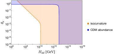
Figure 1: Constraints on $H_{{\rm inf}}$ and $\theta_{a}$ when we assume $F_{a}=10^{12}$ GeV. The orange and blue regions are excluded by the observation of the isocurvature perturbations and cold dark matter abundance respectively.

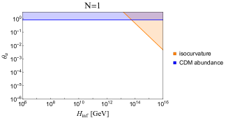
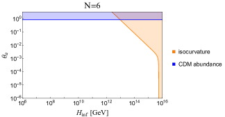
Figure 2: The same constraints as Fig. 1 but with the large value $M_{{\rm pl}}$ of the PQ field during inflation. The left figure shows the $N=1$ case and the right figure shows the $N=6$ case, e.g. the DFSZ model.

III Simulation setup

As seen in the previous section, in the SUSY axion model the isocurvature perturbations are suppressed if the PQ field has a large field value during inflation. However, in this case the PQ field starts to oscillate after inflation and the axion fluctuations grow through parametric resonance. If the fluctuations become sufficiently large, the axion field takes random values in space, which results in the domain wall formation. To examine whether domain walls are formed we perform numerical lattice simulations.

For simplicity, we make the following assumptions through the simulations.

$$\Phi_{0}=0,~{}~{}~{}~{}m\equiv m_{+}=m_{-},~{}~{}~{}~{}~{}h=1.$$ (29)

Then the scalar potential $V$ is written as

$$V=|\Phi_{+}\Phi_{-}-v^{2}|^{2}+m^{2}(|\Phi_{+}|^{2}+|\Phi_{-}|^{2}).$$ (30)

III.1 Equations of motion

We decompose complex scalar fields into their real parts and complex parts,

$$\Phi_{+} =\frac{1}{\sqrt{2}}(\phi_{0}+i\phi_{1}),$$ (31)

$$\Phi_{-} =\frac{1}{\sqrt{2}}(\phi_{2}+i\phi_{3}).$$ (32)

We solve the evolution of the scalar fields taking the cosmic expansion into account. Using the FRW metric $g_{\mu\nu}={\rm diag}(1,\ -R,\ -R,\ -R)$ where $R$ is the scale factor, equations of motion are written as

$$\ddot{\phi}_{i}+3H\dot{\phi}_{i}-\frac{1}{R^{2}}\Delta\phi_{i}+\frac{\partial V(\phi)}{\partial\phi_{i}}=0.\ \ (i=0,1,2,3).$$ (33)

Furthermore, let us rescale the variables as

$$d\tau =m\frac{dt}{R},$$ (34)

$$d\tilde{x} =mdx,$$ (35)

$$\phi_{i} =\frac{m}{R}\varphi_{i}.$$ (36)

Then equations of motion are rewritten as

$$\varphi_{i}^{\prime\prime}-\tilde{\Delta}\varphi_{i}-\frac{R^{\prime\prime}}{R}\varphi_{i}+\frac{\partial V(\varphi)}{\partial\varphi_{i}}=0.$$ (37)

where

$$\frac{\partial V(\varphi)}{\partial\varphi_{0}} =\frac{1}{2}\left[\left(\varphi_{0}\varphi_{2}-\varphi_{1}\varphi_{3}-2\left(\frac{v}{m}R\right)^{2}\right)\varphi_{2}+(\varphi_{0}\varphi_{3}+\varphi_{1}\varphi_{2})\varphi_{3}\right]+a^{2}\varphi_{0},$$ (38)

$$\frac{\partial V(\varphi)}{\partial\varphi_{1}} =\frac{1}{2}\left[-\left(\varphi_{0}\varphi_{2}-\varphi_{1}\varphi_{3}-2\left(\frac{v}{m}R\right)^{2}\right)\varphi_{3}+(\varphi_{0}\varphi_{3}+\varphi_{1}\varphi_{2})\varphi_{2}\right]+a^{2}\varphi_{1},$$ (39)

$$\frac{\partial V(\varphi)}{\partial\varphi_{2}} =\frac{1}{2}\left[\left(\varphi_{0}\varphi_{2}-\varphi_{1}\varphi_{3}-2\left(\frac{v}{m}R\right)^{2}\right)\varphi_{0}+(\varphi_{0}\varphi_{3}+\varphi_{1}\varphi_{2})\varphi_{1}\right]+a^{2}\varphi_{2},$$ (40)

$$\frac{\partial V(\varphi)}{\partial\varphi_{3}} =\frac{1}{2}\left[-\left(\varphi_{0}\varphi_{2}-\varphi_{1}\varphi_{3}-2\left(\frac{v}{m}R\right)^{2}\right)\varphi_{1}+(\varphi_{0}\varphi_{3}+\varphi_{1}\varphi_{2})\varphi_{0}\right]+a^{2}\varphi_{3}.$$ (41)

The prime denotes the derivative with respect to $\tau$. We solve these equations numerically in the lattice simulation.

III.2 Relations between PQ fields and axion

Next, we describe the relations between $\varphi_{0},\ \varphi_{1},\ \varphi_{2},\ \varphi_{3}$ and $\varphi_{\pm},\ a_{\pm}$. They are written as

$$\varphi_{+}^{2} =\left(\frac{1}{\sqrt{2}}\frac{m}{R}\right)^{2}(\varphi_{0}^{2}+\varphi_{1}^{2}),$$ (42)

$$\varphi_{-}^{2} =\left(\frac{1}{\sqrt{2}}\frac{m}{R}\right)^{2}(\varphi_{2}^{2}+\varphi_{3}^{2}).$$ (43)

from Eqs. (13), (31), and (32). Then from Eq. (14),

$$a=\varphi_{\pm}{\rm tan^{-1}\frac{\varphi_{1}}{\varphi_{0}}=\varphi_{\pm}{\rm tan^{-1}\frac{\varphi_{3}}{\varphi_{2}}}}.$$ (44)

Thus the phase angle of the axion field is

$$\theta_{a} =\frac{a}{(\varphi_{+}^{2}+\varphi_{-}^{2})^{1/2}},$$ (45)

$$=\left(\frac{1}{\sqrt{2}}\frac{m}{R}\right)^{-1}\frac{1}{\varphi_{0}^{2}+\varphi_{1}^{2}+\varphi_{2}^{2}+\varphi_{3}^{2}}\left[(\varphi_{0}^{2}+\varphi_{1}^{2})\tan^{-1}\frac{\varphi_{1}}{\varphi_{0}}-(\varphi_{2}^{2}+\varphi_{3}^{2})\tan^{-1}\frac{\varphi_{3}}{\varphi_{2}}\right].$$ (46)

III.3 Simulation condition

In reality, the typical mass scales of $m$ and $v$ are about $10^{3}$ GeV and $10^{12}$ GeV, respectively. However, in numerical simulation it is impossible to study the dynamical system with such hugely different mass scales at the same time. Therefore, we set $v/m$ being as small as to satisfy the condition that the scalar fields are confined in the flat direction. Suppose that $A$ is the initial amplitude of the homogeneous part of $\Phi_{+}$. Then, because the energy density of the orthgonal direction and the PQ field is about $v^{4}$ and $m^{2}(Av)^{2}$, $A$ should satisfy

$$A <\frac{v}{m}.$$ (47)

As for the initial conditions for the scalar fields we take

$$\langle{\rm Re}\Phi_{+}\rangle_{i} =A\times v,$$ (48)

$$\langle{\rm Re}\Phi_{-}\rangle_{i} =\frac{1}{A}\times v,$$ (49)

$$\langle{\rm Im}\Phi_{+}\rangle_{i} =\langle{\rm Im}\Phi_{-}\rangle_{i}=0.$$ (50)

where $i$ denotes the initial values and we changed $A$ in the lattice simulations. We initially assign tiny fluctuations, which are random numbers in $[-10^{-6}\ ,10^{6}]$, to the scalar fields at each lattice point. We assume that the universe is matter dominated and set the initial time $\tau_{i}=1$ and the initial scale factor $R(\tau_{i})=1$, which means $R(\tau)=\tau^{2}$. To study the precise evolution of the PQ field after inflation, we have performed the simulation in 2 dimensions with periodic boundary conditions. For the test of the code we calculate the total energy density of the system without cosmic expansion, which is conserved with accuracy less than 0.2% for $A=100$ and $v/m=500$.

IV Result of the lattice simulation

Table 1: Simulation parameters. $L$ and $N$ are the box size and the number of grid points. $\Delta\tau$ is the time step of the simulation. The box size $L$ is normalized by the oscillation mass scale $m$.

	$A$	$v/m$	$mL$	$N$	$\Delta\tau$
(i)	$100$	$50$	$10$	$512^{2}$	$2\times 10^{-4}$
(ii)	$200$	$100$	$10$	$1024^{2}$	$7\times 10^{-5}$
(iii)	$500$	$200$	$10$	$2200^{2}$	$1\times 10^{-5}$
(iv)	$1000$	$500$	10	$2048^{2}$	$2\times 10^{-6}$

We perform the simulations changing $A$ and the lattice parameters as shown in Table 1. We confirm that the behavior of the system does not change with the different simulation box size $mL$. In this paper, the maximum value of $A$ is $1000$ coming from the limit of the available machine power.

In numerical simulation, the time step must be smaller than any oscillation time scales of the equations of motion. For the equations of motion of $\varphi_{2}$ given by

$$\varphi_{2}^{\prime\prime}-\tilde{\Delta}\varphi_{2}-\frac{R^{\prime\prime}}{R}\varphi_{2}+\frac{\partial V(\varphi)}{\partial\varphi_{2}}=0,$$ (51)

the most important part in the initial configuration is the time derivative of $\varphi_{2}$ and its potential. Then the equation is effectively written as

$$\varphi_{2}^{\prime\prime} \simeq-\frac{\partial V(\varphi)}{\partial\varphi_{2}},$$ (52)

$$=-\frac{1}{2}\left[\left(\varphi_{0}\varphi_{2}-\varphi_{1}\varphi_{3}-2\left(\frac{v}{m}R\right)^{2}\right)\varphi_{0}+(\varphi_{0}\varphi_{3}+\varphi_{1}\varphi_{2})\varphi_{1}\right]-a^{2}\varphi_{2},$$ (53)

$$\simeq-\frac{1}{2}\left(\varphi_{0}^{2}\varphi_{2}-2\left(\frac{v}{m}R\right)^{2}\varphi_{0}\right)-a^{2}\varphi_{2}.$$ (54)

and the largest oscillation time scale of this equation is about $|\varphi_{0}|=A\times v/m$, the first term of Eq. (54). Thus if we perform the simulations with the larger value of $A$ , we have to take smaller value of $\Delta\tau\sim(A\times v/m)^{-1}$, which requires much longer CPU time and hence sets the maximum value of $A$.

Because the epoch of the PQ field oscillation is much earlier than the QCD phase transition, the axion is massless and the axion field tends to be homogeneous inside the horizon due to the gradient term of the equation of motion. Thus, for domain walls to be formed the field value of the axion must be different in each Hubble patch after parametric resonance. Because the box size $L$ of our simulations is smaller than the horizon size $H^{-1}\sim\tau^{3}$ at the end of the simulations, we cannot directly see that the axion field takes different values at different Hubble patches. Thus, to examine whether the domain wall problem arises, we investigate the spatial distribution of the field value of the axion after parametric resonance in the simulation box. If the axion field takes completely random value through parametric resonance, the axion angle $\theta_{a}$ has a flat distribution in $[-\pi,\pi]$ just after the resonance. In the subsequent evolution the gradient term aligns the angle, which leads to the angle distribution with a peak at some value. Once the angle becomes sufficiently random, the peak angle is also random. In other words, if the axion fluctuations do not grow enough, the angle distribution has a peak at the initial value, $\langle\theta_{a}\rangle_{i}=0$.

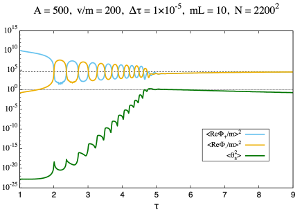
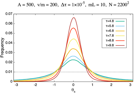
Figure 3: Left: the time evolution of the average of real parts of PQ fields, ${\rm\langle Re}\Phi_{\pm}\rangle$, and the variance of the axion field $\langle\theta_{a}^{2}\rangle$ for the case of (iii) in the Table 1. The broken line shows $v/m$ and the dotted line shows $10^{0}$. Right: the histogram of the spatial distribution of the axion angle $\theta_{a}$. The distribution $f$ is normalized as $\int_{-\pi}^{\pi}fd\theta_{a}=2\pi/100$. The dotted line shows the case where the values of $\theta_{a}$ are completely random.

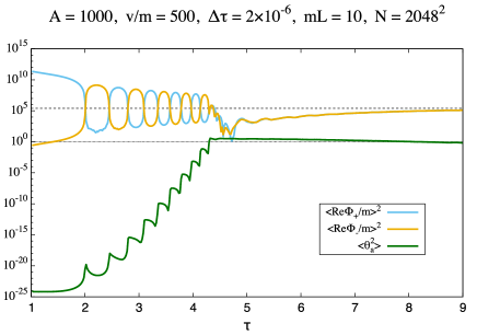
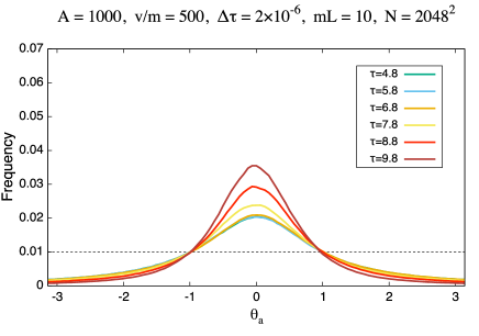
Figure 4: The same as Fig. 3 but for the case of (iv) in the Table 1.

The result of our simulations is shown in Figs. 3 and 4 for $A=500$ and $A=1000$. The left panels of the figures show the average of the $\Phi_{\pm}$ fields, $\langle{\rm Re}\Phi_{\pm}\rangle$, and the variance of the axion angle, $\langle\theta_{a}^{2}\rangle$. We find that the axion fluctuations become large through parametric resonance during the $\Phi_{\pm}$ oscillating. Then at $\tau\simeq 4.8$ the angle fluctuations reach $O(1)$, that means the angle is widely distributed between $-\pi$ and $\pi$. However, afterward the angle is aligned by the gradient term and its fluctuation gradually decrease. This situation is shown in the right panels of the figures where the time evolutions of the angle distributions are shown. In these figures, we divided $-\pi$ to $\pi$ equally into $100$ bins and plot the frequency of the value of $\theta_{a}$ from $\tau\simeq 4.8$ every $\Delta\tau=1$, which corresponds to the point of maximum fluctuations of the axion field. We find that the values of the axion angle come back to the initial one, $\langle\theta_{a}\rangle_{i}=0$. Therefore, domain wall problem does not arise at least for $A\leq 1000$.

In this case the isocurvature perturbation constraint on the Hubble parameter during inflation $H_{\text{inf}}$ is shown as Fig. 5 for $A=1000$ and $F_{a}=10^{12}\ {\rm GeV}$. From the figure we find that the Hubble parameter $H_{{\rm inf}}$ can be as large as $10^{13}$ GeV if the misalignment angle is smaller than about $10^{-3}$. Furthermore if we assume that the axion accounts for all the dark matter of the universe, the relation

$$0.18\times\left[\theta_{a}^{2}+\left(\frac{H_{{\rm inf}}}{2\pi AF_{a}}\right)^{2}\right]\left(\frac{F_{a}}{10^{12}\text{GeV}}\right)^{1.19} =0.12,$$ (55)

holds. Using this equation and Eq. (27), we obtain the constraint on $H_{{\rm inf}}$ and $\theta_{a}$ for $A=1000$ as shown in Fig. 6. In the figure we also show the constraint (gray region) from the requirement that the field value during inflation should be less than $M_{\text{pl}}$, i.e. $Av\lesssim M_{\text{pl}}$. We find that $H_{{\rm inf}}\lesssim 10^{12}\ {\rm GeV}$ for $A=1000$ in the SUSY axion model without the domain wall problem. Thus the axion can be the main component of the dark matter avoiding both domain wall and isocurvautre perturbation problems for $H_{{\rm inf}}\lesssim 10^{12}$ GeV in this model.

As mentioned before, with the present computer power it is difficult to examine whether domain walls are formed clearly for larger $A$. However, results of $A\leq 1000$ imply that the fluctuations of the misalignment angle are not enough to produce domain walls. This is because completely randam spatial distribution of the axion after parametric resonance is needed for the domain wall formation, but the situation is far from this even for $A=1000$ as we can see from Fig. 4. Therefore we expect that the allowed parameter region in Fig. 6 would be extended.

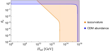
Figure 5: Constraints on $H_{{\rm inf}}$ and $\theta_{a}$ when we use $A=1000$ and $F_{a}=10^{12}$ GeV. The orange and blue regions are excluded by the observation of the isocurvature perturbations and cold dark matter abundance respectively.

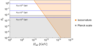
Figure 6: Constraints on $\theta_{a}$ and $H_{\text{inf}}$ for $A=1000$ under the assumption that the axion is the only component of cold dark matter. The gray region is excluded by the condition that $Av=N\times AF_{a}\lesssim M_{{\rm pl}}$ for $N=1$. The blue dotted lines show $F_{a}=10^{12}$ GeV, $F_{a}=10^{14}$ GeV, and $F_{a}=10^{16}$ GeV.

V Conclusion and discussion

In this paper, we have investigated the isocurvature and domain wall problems in the SUSY axion model. If the PQ field has a large field value during inflation the isocuravture perturbations are suppressed. However, after inflation the PQ field starts oscillation and produces large fluctuations of the axion field through parametric resonance, which may lead to the domain wall problem. We have performed the lattice simulations to examine whether the domain wall problem arises. From the result of the simulations, we have found that the domain walls are not formed if the ratio $A$ of the PQ field value $|\Phi_{+}|$ during inflation to the PQ breaking scale $v$ is less than $10^{3}$, i.e. $A=|\Phi_{+}|_{i}/v\leq 10^{3}$. This relaxes the stringent constraint on the Hubble parameter during inflation $H_{\text{inf}}$ as $10^{13}$ GeV for $F_{a}=10^{12}$ GeV. Moreover, if the axion is dark matter, we obtain the constraint on $H_{\text{inf}}$ as $H_{\text{inf}}\lesssim 10^{12}$ GeV.

We could not reach the definite conclusion on the domain wall problem for larger $A$ because more machine power is needed to perform the lattice simulations. However, for domain walls to be formed the spatial distribution of the axion fields must be completely random, which seems unlikely even for larger $A$ judging from the result of our simulations. Therefore, we expect that larger $H_{\text{inf}}$ would be allowed.

References

- Weinberg (1978) S. Weinberg, Phys. Rev. Lett. 40, 223 (1978).
- Wilczek (1978) F. Wilczek, Phys. Rev. Lett. 40, 279 (1978).
- Peccei and Quinn (1977a) R. D. Peccei and H. R. Quinn, Phys. Rev. D16, 1791 (1977a).
- Peccei and Quinn (1977b) R. D. Peccei and H. R. Quinn, Phys. Rev. Lett. 38, 1440 (1977b).
- ’t Hooft (1976) G. ’t Hooft, Phys. Rev. Lett. 37, 8 (1976).
- Preskill et al. (1983) J. Preskill, M. B. Wise, and F. Wilczek, Phys. Lett. 120B, 127 (1983).
- Abbott and Sikivie (1983) L. F. Abbott and P. Sikivie, Phys. Lett. 120B, 133 (1983).
- Dine and Fischler (1983) M. Dine and W. Fischler, Phys. Lett. 120B, 137 (1983).
- Sikivie (1982) P. Sikivie, Phys. Rev. Lett. 48, 1156 (1982).
- Vilenkin and Everett (1982) A. Vilenkin and A. E. Everett, Phys. Rev. Lett. 48, 1867 (1982).
- Hiramatsu et al. (2012) T. Hiramatsu, M. Kawasaki, K. Saikawa, and T. Sekiguchi, Phys. Rev. D85, 105020 (2012), [Erratum: Phys. Rev.D86,089902(2012)], arXiv:1202.5851 [hep-ph] .
- Ryden et al. (1989) B. S. Ryden, W. H. Press, and D. N. Spergel, Submitted to: Astrophys. J. (1989).
- Axenides et al. (1983) M. Axenides, R. H. Brandenberger, and M. S. Turner, Phys. Lett. 126B, 178 (1983).
- Seckel and Turner (1985) D. Seckel and M. S. Turner, Phys. Rev. D32, 3178 (1985).
- Linde (1985) A. D. Linde, Phys. Lett. 158B, 375 (1985).
- Linde and Lyth (1990) A. D. Linde and D. H. Lyth, Phys. Lett. B246, 353 (1990).
- Turner and Wilczek (1991) M. S. Turner and F. Wilczek, Phys. Rev. Lett. 66, 5 (1991).
- Lyth (1992) D. H. Lyth, Phys. Rev. D45, 3394 (1992).
- Ade et al. (2016) P. A. R. Ade et al. (Planck), Astron. Astrophys. 594, A20 (2016), arXiv:1502.02114 [astro-ph.CO] .
- Linde (1991) A. D. Linde, Phys. Lett. B259, 38 (1991).
- Kofman et al. (1996) L. Kofman, A. D. Linde, and A. A. Starobinsky, Phys. Rev. Lett. 76, 1011 (1996), arXiv:hep-th/9510119 [hep-th] .
- Kofman et al. (1997) L. Kofman, A. D. Linde, and A. A. Starobinsky, Phys. Rev. D56, 3258 (1997), arXiv:hep-ph/9704452 [hep-ph] .
- Shtanov et al. (1995) Y. Shtanov, J. H. Traschen, and R. H. Brandenberger, Phys. Rev. D51, 5438 (1995), arXiv:hep-ph/9407247 [hep-ph] .
- Tkachev et al. (1998) I. Tkachev, S. Khlebnikov, L. Kofman, and A. D. Linde, Phys. Lett. B440, 262 (1998), arXiv:hep-ph/9805209 [hep-ph] .
- Kasuya and Kawasaki (1998) S. Kasuya and M. Kawasaki, Phys. Rev. D58, 083516 (1998), arXiv:hep-ph/9804429 [hep-ph] .
- Kasuya and Kawasaki (2000) S. Kasuya and M. Kawasaki, Phys. Rev. D61, 083510 (2000), arXiv:hep-ph/9903324 [hep-ph] .
- Kawasaki et al. (2013) M. Kawasaki, T. T. Yanagida, and K. Yoshino, JCAP 1311, 030 (2013), arXiv:1305.5338 [hep-ph] .
- Kasuya et al. (1997) S. Kasuya, M. Kawasaki, and T. Yanagida, Phys. Lett. B409, 94 (1997), arXiv:hep-ph/9608405 [hep-ph] .
- Dine et al. (1995) M. Dine, L. Randall, and S. D. Thomas, Phys. Rev. Lett. 75, 398 (1995), arXiv:hep-ph/9503303 [hep-ph] .
- Gaillard et al. (1995) M. K. Gaillard, H. Murayama, and K. A. Olive, Phys. Lett. B355, 71 (1995), arXiv:hep-ph/9504307 [hep-ph] .
- Kim (1979) J. E. Kim, Phys. Rev. Lett. 43, 103 (1979).
- Shifman et al. (1980) M. A. Shifman, A. I. Vainshtein, and V. I. Zakharov, Nucl. Phys. B166, 493 (1980).
- Dine et al. (1981) M. Dine, W. Fischler, and M. Srednicki, Phys. Lett. 104B, 199 (1981).
- Zhitnitsky (1980) A. R. Zhitnitsky, Sov. J. Nucl. Phys. 31, 260 (1980), [Yad. Fiz.31,497(1980)].
- Kim and Nilles (1984) J. E. Kim and H. P. Nilles, Phys. Lett. 138B, 150 (1984).