Continuous groupoids on the symbolic space, quasi-invariant probabilities for Haar systems and the Haar-Ruelle operator

Abstract

We consider groupoids on $\{1,2,..,d\}^{\mathbb{N}}$, cocycles and the counting measure as transverse function. We generalize results relating quasi-invariant probabilities with eigenprobabilities for the dual of the Ruelle operator. We assume a mild compatibility of the groupoid with the symbolic structure. We present a generalization of the Ruelle operator - the Haar-Ruelle operator - taking into account the Haar structure. We consider continuous and also Hölder cocycles. IFS with weights appears in our reasoning in the Hölder case.

   

1 Introduction

The symbolic space $X=\{1,2,...,d\}^{\mathbb{N}}$ is a compact metric space for the usual metric $d$ described on [16]. The shift $\sigma$ acts on this space as a continuous transformation.

We introduce an equivalence relation $\sim$ in $X$, such that, the map $x\to[x]:=\{s\in X|s\sim x\}$ is hemicontinuous, as a multivalued function (see [1], Section 17.2, for details on hemicontinuity and nets).

Definition 1.1.

Given an equivalence relation $\sim$ we consider the associated groupoid

$$G=\{\,\,(x,y)\in X^{2}\,\,\text{such that}\,\,x\sim y\,\,\},$$

and, as usual we denote $G^{0}=\{\,\,(x,x)\in G\,\,\text{such that}\,\,x\in X\,\,\,\}\cong X$.

We identify $X$ with $G^{0}$.

We consider over $G$ the topology induced by the product topology on $X^{2}$. $\mathcal{B}$ denotes the Borel sigma-algebra on $G$.

In general groupoids are equipped with some algebraic structure (see [7] or [17]) but this will not be relevant for our purposes (see discussion on [3]).

Definition 1.2.

A measurable (continuous) groupoid $G$ is a groupoid, such that,

$P_{1}(x,y)=x$, $\,P_{2}(x,y)=y$, $\,h(x,y)=(y,x)$ and $Z(\,(x,s),(s,y)\,)=(x,y),$ are Borel measurable (continuous).

Definition 1.3.

A transverse function $\nu$ on the measurable groupoid $G$ is a map of $X$ in the space of measures over the sigma-algebra $\mathcal{B}$, such that,

1) $\forall y\in X$, the measure $\nu^{y}$ has support on $[y]$,

2) $\forall A\in\mathcal{B}$, we have that $\nu^{y}(A)$, as a function of $y$, is measurable.

3) for any $r,s\in[y]$ we have that $\nu^{s}=\nu^{r}.$

General references on groupoids and transverse functions for an Ergodic Theory audience are [12] and [3].

The only transverse function $\nu$ we will consider here is the counting measure.

Definition 1.4.

Given the transverse function $\nu$ described above over the measurable groupoid $G$ we consider the Haar system $(G,\nu)$, where $\mathop{\rm supp}\nolimits\nu^{x}=[x]$ and $\nu^{x}=\nu^{y}$, when $x\sim y$. We assume also that $\nu^{x}([x])\leq\infty$.

A modular function $\delta:G\to\mathbb{R}$ is a continuous function, such that, $\delta(x,z)=\delta(x,y)\,\delta(y,z),\forall x\sim y\sim z\in X$ (see section 3 in [7]).

Definition 1.5.

$c:G\to\mathbb{R}$ is a cocycle, if $c(x,z)=c(x,y)+c(y,z),\forall x\sim y\sim z\in X$. Therefore, $\delta(x,y)=e^{\beta c(y,x)}=e^{-\beta c(x,y)}$ is a modular function, for any $\beta\in\mathbb{R}$.

We define $\mathcal{C}_{\sim}=\{c:G\to\mathbb{R}\,\,|\,\,\text{ c is a cocycle for }\sim\}$.

We claim that $\mathcal{C}_{\sim}$ is a linear space. Indeed, given $c,b\in\mathcal{C}_{\sim}$ and $\alpha\in\mathbb{R}$ we have

$$(c+\alpha b)(x,z)=c(x,z)+\alpha b(x,z)=c(x,y)+c(y,z)+\alpha(b(x,y)+b(y,z))=$$

$$=c(x,y)+\alpha b(x,y)+c(y,z)+\alpha b(y,z)=(c+\alpha b)(x,y)+(c+\alpha b)(y,z),$$

and, $0\in\mathcal{C}_{\sim}$.

Definition 1.6.

We call coboundary a function of the form $V(y)-V(x)\in\mathcal{C}_{\sim}$, for some $V:G^{0}\to\mathbb{R}$. Given $c_{0}\in\mathcal{C}_{\sim}$, we say that $c$ is cohomologous to $c_{0}$, if $c(x,y)=c_{0}(x,y)+V(y)-V(x)$.

Definition 1.7.

We say that a cocycle $c$ is separable if it is cohomologous to $0$, that is,

$$c(x,y)=0+V(y)-V(x)=V(y)-V(x).$$

Motivated by examples in Statistical Mechanics and Quantum Field Theory, the authors Kubo, Martin and Schwinger introduce the concept of KMS state on a $C^{*}$-Algebra or on a Von Neumann Algebra. They describe on Quantum Statistical Physics the role of the Gibbs state (see [3] or [17]).

A large class of Von Neumann Algebras are defined from measurable groupoids and Haar systems. A cocycle - in some sense - plays in this setting the role of the external potential in Statistical Mechanics.

The quasi-invariant condition for a probability $M$ on $X$ (to be defined next) is related to the so called KMS-condition and to KMS states on von Neumann algebras or $C^{*}$ algebras (see [3], [8], [9] or [17]).

We will be interested here in quasi-invariant probabilities for a certain family of groupoids and a certain kind of cocycle (see Definition 2.3.8. in [17]). It will be not necessary to talk about KMS states.

Definition 1.8.

Given a cocycle $c$ we say that probability $M$ over the Borel sets of $X$ satisfies the $(c,\ \beta)-$quasi-invariant condition for the grupoid $(G,\ \nu)$, if for any integrable function $h:G\rightarrow\mathbb{R}$, we have

$$\int\int h(s,\ x)d\nu^{x}(s)dM(x)=\int\int h(x,\ s)e^{-\beta c(x,s)}d\nu^{x}(s)dM(x),$$ (1)

where $\beta\in\mathbb{R}$ and $c:G\rightarrow\mathbb{R}.$

A natural question is: given a cocycle $c$ is there a relation of the associated quasi-stationary probability $M$ (which is defined by (1)) with the Gibbs state (for some potential) of Statistical Mechanics? The answer is yes and this is the primary interest here. Our main results are Theorems 2.3, 3.5, 4.6 and Proposition 6.1.

One of our purposes here is to show the relation of quasi-invariant probabilities with eigenprobabilities of the dual of a general form of Ruelle operator (which takes into account the transverse function $\nu$). A particular case of this kind of result appears on section 4 in [3] which deals with the Classical Thermodynamic Formalism (see [16]). References for different forms of Ruelle operators (some of them for IFSw) are [2], [6], [10], [14] and [15].

Among other things we will consider here the Haar-Ruelle operator (see Definition 2.1) which is a natural concept to consider in the present setting.

We point out that the results about quasi-stationary probabilities of [11] and [17] (on the setting of $C^{*}$-Algebras) have a different nature of the ones we consider here (there, for instance, for just one value of $\beta$ you get a quasi-invariant probability - Theorem 3.5 in [11]). Moreover, in [11] for such value of $\beta$ the KMS (quasi-invariant) probability for the $C^{*}$ algebra is unique. Here the results are for any $\beta$ and quasi-invariant probabilities are not unique.

We will consider here a more general class of groupoids than [3]. We will present in Example 4.7 the expression of the quasi-invariant probability for a certain cocycle using an iteration method which follow from our reasoning. This is particularly important for results related to spectral triples (see [5])

In order to obtain a connection between the groupoid (the Haar system) and the symbolic structure on $X$ we will require a mild compatibility hypothesis on the equivalence relation $\sim$.

We recall that $X=\{1,2,...,d\}^{\mathbb{N}}$ and the operation $i*x=(i,x_{1},x_{2},...)$ is the concatenation of the symbol $i$ in the first position displacing all the symbols in $x=(x_{1},x_{2},...)$.

Definition 1.9.

We say that the equivalence relation $\sim$ is continuous with respect to the symbolic structure if, for all $x\in X$, the set given by

$$\{1*x,...,d*x\}\in X^{d}$$

has a continuous representation $\psi$ of its classes, $j*x\stackrel{{\scriptstyle\psi}}{{\to}}[j*x]$, in the following sense:

First note that $\psi(j*x)$ is an $k$-uple (where $k$ is the cardinality of $[j*x]$). We assume it is well defined an ordered string $\{\psi_{1}(j*x),...,\psi_{k}(j*x)\}$.

$\forall\varepsilon>0$, there exists $\delta>0$, such that, if $d(x,z)<\delta$ and

$$[j*x]=\{\psi_{1}(j*x),...,\psi_{k}(j*x)\}$$

$$[j*z]=\{\psi_{1}(j*z),...,\psi_{k}(j*z)\},$$

then, $\displaystyle\max_{i=1..k}d(\psi_{i}(j*x),\psi_{i}(j*z))<\varepsilon$, where $k=\sharp[j*x]=\sharp[j*z]$.

For a Lipschitz relation $\sim$ will be required that for $\psi$:

$$\max_{i=1,...,k}d(\psi_{i}(j*x),\psi_{i}(j*z))<rd(x,z),$$

in particular, $Lip(\psi_{i}(j*x))\leq r$, for all $i,j$.

Definition 1.10.

A groupoid $G$ associated to a continuous equivalence $\sim$ relation will be called a continuous groupoid. A Lipschitz groupoid is defined on a similar manner.

We assume from now on that $G$ is at least a continuous groupoid.

Proposition 1.11.

The representation $\psi$ has the absorbtion property

$$\psi_{a}(\psi_{b}(x))=\psi_{a}(x),$$

for all $x\in X$.

Proof. The proof is obvious from the definition because $[\psi_{b}(x)]=[x]$ and $\psi_{a}$ returns the $a$-nth element in this class which is $\psi_{a}(x)$. $\blacksquare$

Example 1.12.

The equivalence relation, $x\sim y\Leftrightarrow\sigma x=\sigma y$, is continuous with respect to the dynamic $\sigma$ because the correspondence

$$j*x\stackrel{{\scriptstyle\psi}}{{\to}}[j*x]=\{1*x,...,d*x\}$$

is constant, given by, $\psi_{i}(j*x):=i*x,$ for all $j$.

2 Non-separable cocycles and the Haar-Ruelle operator

Definition 2.1.

Let $\varphi(x,y)$ be a continuous function in $G$. We introduce the Haar-Ruelle operator, $L_{\varphi}$ as the operator

$$L_{\varphi}(f)(x)=\frac{1}{d}\sum_{j=1}^{d}\int_{[j*x]}f(s)\,e^{\varphi(j*x,s)}d\nu^{j*x}(s),$$

acting onfunctions $f:X\to\mathbb{R}$, integrable with respect to the transverse function $\nu$.

Example 3.2 will show the evidence that we are considering above a generalization of the classical Ruelle operator.

Let $c(x,y)$ be a general (continuous, Lipschitz, Hölder) cocycle (that is, we do not require that $c(x,y)=V(y)-V(x)$). We introduce the Haar-Ruelle operator, $L_{-\beta c}$ by choosing $\varphi=-\beta c$ in Definition 2.1, that is,

$$L_{-\beta c}(f)(x)=\frac{1}{d}\sum_{j=1}^{d}\int_{[j*x]}f(s)\,e^{-\beta c(j*x,s)}d\nu^{j*x}(s),$$

for any integrable $f:X\to\mathbb{R}$.

We recall that $[j*x]=\{\psi_{1}(j*x),...,\psi_{k}(j*x)\}$ and $\nu^{j*x}$ is the counting measure so the Haar-Ruelle operator takes the form:

$$L_{-\beta c}(f)(x)=\frac{1}{d}\sum_{j=1}^{d}\sum_{i=1}^{k}f(\psi_{i}(j*x))\,e^{-\beta c(j*x,\ \psi_{i}(j*x))}.$$

All of our results are true for any $\beta>0$.

As usual the dual $L^{*}$ of an operator $L$ acting on continuous function acts on measures (see [16]).

Theorem 2.2.

Consider the Haar-Ruelle operator, $L_{-\beta c}$. Then,
a) $L_{-\beta c}$ is positive and preserves $C^{0}$,
b) There exists $\lambda>0$ and a eigenmeasure $M$, such that, $L_{-\beta c}^{*}M=\lambda M$.

Proof. (a) It is easy to see that $L_{-\beta c}$ is positive and $L_{-\beta c}$ is just the sum of the composition of continuous functions.

(b) It is a direct application of the Tychonoff-Schauder theorem to the continuous operator $T$ given by

$$T(\mu)=\frac{1}{\int_{X}L_{-\beta c}(1)(x)d\mu(x)}L_{-\beta c}^{*}(\mu).$$

Therefore, there exists $\mu$ such that $T(\mu)=\mu$, in other words, $\mu$ satisfies

$$\frac{1}{\int_{X}L_{-\beta c}(1)(x)d\mu(x)}L_{-\beta c}^{*}(\mu)=\mu.$$

Finally, take

$$M=\mu\text{ and }\lambda=\int_{X}L_{-\beta c}(1)(x)d\mu(x)>0.$$

$\blacksquare$

Theorem 2.3.

Let $M$ be a measure such that $L_{-\beta c}^{*}M=\lambda M$, $\lambda>0$. Then, $M$ is quasi-invariant.

Proof.

The quasi-invariant equation, when $\nu^{x}$ is the counting measure is

$$\int\sum_{t=1}^{k}h(\psi_{t}(x),\ x)dM(x)=\int\sum_{t=1}^{k}h(x,\ \psi_{t}(x))e^{-\beta c(x,\ \psi_{t}(x))}dM(x),$$

which is equivalent to

$$\int f(x)dM(x)=\int g(x)dM(x)$$

$$\int f(x)\lambda dM(x)=\int g(x)\lambda dM(x)$$

$$\int f(x)dL_{-\beta c}^{*}M(x)=\int g(x)dL_{-\beta c}^{*}M(x)$$

$$\int L_{-\beta c}(f)(x)dM(x)=\int L_{-\beta c}(g)(x)dM(x),$$

where $f(x):=\sum_{t=1}^{k}h(\psi_{t}(x),\ x)$ and $g(x):=\sum_{t=1}^{k}h(x,\ \psi_{t}(x))e^{-\beta c(x,\ \psi_{t}(x))}$.

We will evaluate $A=L_{-\beta c}(f)(x)$ and $B=L_{-\beta c}(g)(x)$:

$$A=L_{-\beta c}(f)(x)=\frac{1}{d}\sum_{j=1}^{d}\sum_{i=1}^{k}f(\psi_{i}(j*x))\,e^{-\beta c(j*x,\ \psi_{i}(j*x))}=$$

$$=\frac{1}{d}\sum_{j=1}^{d}\sum_{i=1}^{k}\sum_{t=1}^{k}h(\psi_{t}(\psi_{i}(j*x)),\ \psi_{i}(j*x))\,e^{-\beta c(j*x,\ \psi_{i}(j*x))}=$$

$$=\frac{1}{d}\sum_{j=1}^{d}\sum_{i=1}^{k}\sum_{t=1}^{k}h(\psi_{t}(j*x)),\ \psi_{i}(j*x))\,e^{-\beta c(j*x,\ \psi_{i}(j*x))},$$

because we can take $\psi_{t}(\psi_{i}(j*x))=\psi_{t}(j*x)$ (from Proposition 1.11).

On the other hand

$$B=L_{-\beta c}(g)(x)=\frac{1}{d}\sum_{j=1}^{d}\sum_{i=1}^{k}g(\psi_{i}(j*x))\,e^{-\beta c(j*x,\ \psi_{i}(j*x))}=$$

$$=\frac{1}{d}\sum_{j=1}^{d}\sum_{i=1}^{k}\sum_{t=1}^{k}h(\psi_{i}(j*x),\ \psi_{t}(\psi_{i}(j*x)))e^{-\beta c(\psi_{i}(j*x),\ \psi_{t}(\psi_{i}(j*x)))}\,e^{-\beta c(j*x,\ \psi_{i}(j*x))}=$$

$$=\frac{1}{d}\sum_{j=1}^{d}\sum_{i=1}^{k}\sum_{t=1}^{k}h(\psi_{i}(j*x),\ \psi_{t}(\psi_{i}(j*x)))e^{-\beta c(j*x,\ \psi_{t}(\psi_{i}(j*x)))}=$$

$$=\frac{1}{d}\sum_{j=1}^{d}\sum_{i=1}^{k}\sum_{t=1}^{k}h(\psi_{i}(j*x),\ \psi_{t}(j*x))e^{-\beta c(j*x,\ \psi_{t}(j*x))},$$

because we can take $\psi_{t}(\psi_{i}(j*x))=\psi_{t}(j*x)$ (from Proposition 1.11).

We claim that, for each $1\leq j\leq d$ we have

$$\sum_{i=1}^{k}\sum_{t=1}^{k}h(\psi_{t}(j*x)),\ \psi_{i}(j*x))\,e^{-\beta c(j*x,\ \psi_{i}(j*x))}=$$

$$\sum_{i=1}^{k}\sum_{t=1}^{k}h(\psi_{i}(j*x),\ \psi_{t}(j*x))e^{-\beta c(j*x,\ \psi_{t}(j*x))},$$

so $A=B$. Indeed, for each $1\leq j\leq d$ we have the equality by changing the role of $t$ and $i$, and this proves our claim. $\blacksquare$

Corollary 2.4.

If $c$ is continuous, the measure $M$, given by Theorem 2.2 is $(c,\beta)-$quasi-invariant.

3 Separable cocycles

For separable cocycles we can find quasi-invariant measures by means of a more simple operator. To do that we rewrite the quasi-invariant condition

$$\int\int h(s,\ x)d\nu^{x}(s)dM(x)=\int\int h(x,\ s)e^{-\beta(V(s)-V(x))}d\nu^{x}(s)dM(x)$$

on the form

$$\int\int g(s,\ x)e^{-\beta V(s)}d\nu^{x}(s)dM(x)=\int\int g(x,\ s)e^{-\beta V(s)}d\nu^{x}(s)dM(x),$$

by taking $h(s,x):=g(s,\ x)e^{-\beta V(s)}$. Using the fact that the measure $\nu^{x}$ is the counting measure we obtain

$$\int\sum_{t=1}^{k}g(\psi_{t}(x),\ x)e^{-\beta V(\psi_{t}(x))}dM(x)=\int\sum_{t=1}^{k}g(x,\ \psi_{t}(x))e^{-\beta V(\psi_{t}(x))}dM(x).$$

By abuse of language if $M$ is quasi-invariant for $c(x,y)=V(y)-V(x)$ we may say that $M$ is quasi-invariant for $V$.

Definition 3.1.

Let $c(x,y)=V(y)-V(x)$ be a separable cocycle, for a continuous (or, Hölder) potential $V$. We introduce the separable Haar-Ruelle operator, $L_{-\beta V}$ by choosing $\varphi(x,y)=-\beta V(y)$ that is,

$$L_{-\beta V}(f)(x)=\frac{1}{d}\sum_{j=1}^{d}\int_{s\in[j*x]}f(s)\,e^{-\beta V(s)}d\nu^{j*x}(s),$$

for any integrable $f:X\to\mathbb{R}$.

Example 3.2.

In the case $x\sim y\Leftrightarrow\sigma x=\sigma y$, and $\nu^{j*x}$ being the counting measure, we get that the separable Haar-Ruelle operator is

$$L_{-\beta V}(f)(x)=\frac{1}{d}\sum_{j=1}^{d}\sum_{i=1}^{d}f(i*x)\,e^{-\beta V(i*x)}=\sum_{i=1}^{d}f(i*x)\,e^{-\beta V(i*x)},$$

which is the classical Ruelle operator associated to the potential $-\beta\,V$.

The same arguments used in Theorem 2.2 proves the next theorem in the separable case.

Theorem 3.3.

Assuming that $V$ is just continuous consider the separable Haar-Ruelle operator, $L_{-\beta V}$. Then,
a) $L_{-\beta V}$ is positive and preserves $C^{0}$,
b) There exists an eigenmeasure $M$, such that, $L_{-\beta V}^{*}M=\lambda M$, for some positive value $\lambda$.

We will present an specific example which will help the reader in understanding how the above theorem can be applied for getting quasi-stationary probabilities on our setting.

Example 3.4.

In this example, the equivalence relation $x\sim y\Leftrightarrow x_{i}=y_{i},i\neq 1\text{ and }3$, is continuous with respect to the symbolic structure because the correspondence $k*x\stackrel{{\scriptstyle\psi}}{{\to}}[k*x]$ is given by,

$$\psi_{ij}(k*x)=\psi_{ij}((k,x_{1},x_{2},x_{3},...))=(i,x_{1},j,x_{3},...)\,,\,1\leq i,j\leq d,$$

for all $1\leq k\leq d$. Notice that $\sharp[y]=d^{2}$ for all $y$ and $\sigma(i,x_{1},j,x_{3},...)=x$ only if $j=x_{2}$.

Figure 1: Description of $[k*x]=\{(i,x_{1},j,x_{3},...)|1\leq i,j\leq d\}$, for $d=3$.

In this case, $\nu^{k*x}$ being the counting measure, the Haar-Ruelle operator will be,

$$L_{-\beta V}(f)(x)=\frac{1}{d}\sum_{k=1}^{d}\int_{s\in[k*x]}f(s)\,e^{-\beta V(s)}d\nu^{k*x}(s)=$$

$$=\sum_{i,j=1}^{d}f((i,x_{1},j,x_{3},...))\,e^{-\beta V((i,x_{1},j,x_{3},...))}=$$

$$=\sum_{i,j=1}^{d}f(\tau_{ij}(x))\,e^{-\beta V(\tau_{ij}(x))}.$$

This is exactly the Hutchinson-Barnsley operator for a contractive (${\rm Lip}(\tau_{ij})=1/8$) IFSw $(\Sigma,\tau_{ij},q_{ij})$, where $\tau_{ij}(x)=(i,x_{1},j,x_{3},...)$ and $q_{ij}(x)=e^{-\beta V(\tau_{ij}\,\,x)}$.

By Theorem 4.1, there is a unique positive function $\varphi$ such that $L_{-\beta V}(\varphi)(x)=\lambda\varphi$ and a measure $\mu$ such that $L_{-\beta V}^{*}(\mu)=\lambda\mu$. We claim that $M=\mu$ is a quasi-invariant measure.

Using the fact that $\nu^{x}$ is the counting measure and

$$[x]=\{(r,x_{2},t,x_{4},...)|1\leq r,t\leq d\}$$

we must to prove that for any $g$

$$\int\sum_{r,t=1}^{d}g((r,x_{2},t,x_{4},...),\ x)e^{-\beta V((r,x_{2},t,x_{4},...))}dM(x)=$$

$$\int\sum_{r,t=1}^{d}g(x,\ (r,x_{2},t,x_{4},...))e^{-\beta V((r,x_{2},t,x_{4},...))}dM(x).$$ (2)

Multiplying each side by $\lambda$ and assuming that $L_{-\beta V}^{*}(M)=\lambda M$ we rewrite the lhs of the above equation as

$$A:=\int\sum_{r,t=1}^{d}g((r,x_{2},t,x_{4},...),\ x)e^{-\beta V((r,x_{2},t,x_{4},...))}\lambda dM(x)=$$

$$=\int L_{-\beta V}\sum_{r,t=1}^{d}g((r,x_{2},t,x_{4},...),\ x)e^{-\beta V((r,x_{2},t,x_{4},...))}dM(x)=$$

$$=\int\sum_{y=\tau_{ij}(x)}\sum_{r,t=1}^{d}g((r,y_{2},t,y_{4},...),\ y)e^{-\beta V((r,y_{2},t,y_{4},...))}\,e^{-\beta V(y)}dM(x),$$

where $y=\tau_{ij}(x)=(i,x_{1},j,x_{3},...)$, so $y_{2}=x_{1}$ and $y_{4}=x_{3}$, etc.

Thus, we get

$$A=\int\sum_{i,j=1}^{d}\sum_{r,t=1}^{d}g((r,x_{1},t,x_{3},...),\ (i,x_{1},j,x_{3},...))e^{-\beta V((r,x_{1},t,x_{3},...))}$$

$$\,e^{-\beta V((i,x_{1},j,x_{3},...))}dM(x).$$

Rewriting the rhs of the equation (2) we get

$$B:=\int\sum_{r,t=1}^{d}g(x,\ (r,x_{2},t,x_{4},...))e^{-\beta V((r,x_{2},t,x_{4},...))}\lambda dM(x)=$$

$$=\int\sum_{i,j=1}^{d}\sum_{r,t=1}^{d}g((i,x_{1},j,x_{3},...),\ (r,x_{1},t,x_{3},...))e^{-\beta V((i,x_{1},j,x_{3},...))}$$

$$\,e^{-\beta V((r,x_{1},t,x_{3},...))}dM(x).$$

Thus, $A=B$, and this shows that $M$ is a quasi-invariant probability.

Returning to the general case and inspired by the Example 3.4 we will obtain a fundamental result.

Theorem 3.5.

Let $M$ be a measure such that $L_{-\beta V}^{*}M=\lambda M$, $c(x,y)=V(y)-V(x)$ a separable cocycle and $V$ a continuous function. Then, $M$ is quasi-invariant for $c$.

Proof. As $c$ is a separable cocycle, we have to prove that

$$\int\sum_{t=1}^{k}h(\psi_{t}(x),\ x)e^{-\beta V(\psi_{t}(x))}dM(x)=\int\sum_{t=1}^{k}h(x,\ \psi_{t}(x))e^{-\beta V(\psi_{t}(x))}dM(x).$$

Assume that $L_{-\beta V}^{*}M=\lambda M$ (by Theorem 3.3). The quasi-invariant condition is equivalent to

$$\int f(x)dM(x)=\int g(x)dM(x)$$

$$\int f(x)\lambda dM(x)=\int g(x)\lambda dM(x)$$

$$\int f(x)dL_{-\beta V}^{*}M(x)=\int g(x)dL_{-\beta V}^{*}M(x)$$

$$\int L_{-\beta V}(f)(x)dM(x)=\int L_{-\beta V}(g)(x)dM(x),$$

where

$$f(x):=\sum_{t=1}^{k}h(\psi_{t}(x),\ x)e^{-\beta V(\psi_{t}(x))}$$

and

$$g(x)=\sum_{t=1}^{k}h(x,\ \psi_{t}(x))e^{-\beta V(\psi_{t}(x))}.$$

We will evaluate $A=L_{-\beta V}(f)(x)$ and $B=L_{-\beta V}(g)(x)$:

$$A=L_{-\beta V}(f)(x)=\frac{1}{d}\sum_{j=1}^{d}\sum_{i=1}^{k}f(\psi_{i}(j*x))\,e^{-\beta V(\psi_{i}(j*x))}=$$

$$=\frac{1}{d}\sum_{j=1}^{d}\sum_{i=1}^{k}\sum_{t=1}^{k}h(\psi_{t}(\psi_{i}(j*x)),\ \psi_{i}(j*x))e^{-\beta V(\psi_{t}(\psi_{i}(j*x)))}\,e^{-\beta V(\psi_{i}(j*x))}=$$

$$=\frac{1}{d}\sum_{j=1}^{d}\sum_{i=1}^{k}\sum_{t=1}^{k}h(\psi_{t}(j*x)),\ \psi_{i}(j*x))\,e^{-\beta(V(\psi_{t}(j*x))+V(\psi_{i}(j*x)))},$$

because we can take $\psi_{t}(\psi_{i}(j*x))=\psi_{t}(j*x)$   (from Proposition 1.11).

On the other hand, by an analogous computation

$$B=L_{-\beta V}(g)(x)=\frac{1}{d}\sum_{j=1}^{d}\sum_{i=1}^{k}g(\psi_{i}(j*x))\,e^{-\beta V(\psi_{i}(j*x))}=$$

$$=\frac{1}{d}\sum_{j=1}^{d}\sum_{i=1}^{k}\sum_{t=1}^{k}h(\psi_{i}(j*x)),\ \psi_{t}(j*x))\,e^{-\beta(V(\psi_{i}(j*x)))+V(\psi_{t}(j*x))},$$

because we can take $\psi_{t}(\psi_{i}(j*x))=\psi_{t}(j*x)$  (from Proposition 1.11).

Obviously $A=B$ which proves our claim. $\blacksquare$

Remark 3.6.

We observe that in Corollary 3.7, the measure $M_{0}$ such that $L_{-\beta V}^{*}M_{0}=\lambda_{0}M_{0}$, given by Theorem 3.3, is quasi-invariant. In other words, we proved that

$$\int\sum_{t=1}^{k}h(\psi_{t}(x),\ x)e^{-\beta V(\psi_{t}(x))}dM_{0}(x)=\int\sum_{t=1}^{k}h(x,\ \psi_{t}(x))e^{-\beta V(\psi_{t}(x))}dM_{0}(x).$$

However, $L_{-\beta c}^{*}M_{1}=\lambda_{1}M_{1}$ by Theorem 2.2 and, moreover, by Corollary 2.4 $M_{1}$ is quasi-invariant, that is

$$\int\sum_{t=1}^{k}h(\psi_{t}(x),\ x)dM_{1}(x)=\int\sum_{t=1}^{k}h(x,\ \psi_{t}(x))e^{-\beta(V(\psi_{t}(x))-V(x))}dM_{1}(x),$$

because $c(x,y)=V(y)-V(x)$.

Thus, $M_{0}$ and $M_{1}$ are quasi-invariant measures for the same separable cocycle $c(x,y)=V(y)-V(x)$ and they are not necessarily equal (they are eigenmeasures of different operators). This abundance of quasi-invariant measures will be explored in the next section. Note that for the more particular groupoid considered on the setting of [3] it is also shown that the quasi-invariant probability is not unique (there the cocycle was Holder). The groupoid $G$ of the mentioned result on [3] is the one presented in Example 3.2 (a continuous groupoid).

Corollary 3.7.

If $V$ is in continuous, the measure $M$, such that, $L_{-\beta V}^{*}M=\lambda M$, is quasi-invariant for the associated $c$.

For the proof see Theorem 3.5 (note that $M$ exists by Theorem 3.3).

4 Quasi-invariant measures arising from IFS

On this section we will assume some more regularity on the cocycle.

The terminology IFSw (IFS with weights) was introduced in [13] and [6] for the case of a IFS where the weights are not normalized. This case was also considered in [10] without giving a special name.

We recall a fundamental result on the Hutchinson-Barnsley operator for an IFSw (see [10]).

Theorem 4.1.

Suppose $0\leq j\leq n-1$ and $R=(Y,\tau_{j},q_{j})$ an IFSw satisfying the following hypothesis
a) $\tau_{j}$ is a contraction and
b) each $q_{j}$ is Dini continuous that is, $\displaystyle\int_{0}^{1}\max_{d(x,y)\leq t}\frac{|\ln q_{j}(x)-\ln q_{j}(y)|}{t}dt<+\infty$
and $\rho>0$, the spectral radius of $\displaystyle B_{R}(f)(x)=\sum_{j=0}^{n-1}q_{j}(x)f(\tau_{j}x)$, restricted to the attractor $K$ of $\mathcal{R}=(Y,\tau_{j})$, where

$$\bigcup_{j=0}^{n-1}\tau_{j}(K)=K,$$

then, there exists a unique $h>0$ and a unique $\mu\in M(K)$, such that,

$$B_{R}(h)=\rho\,h\;\mathcal{L}_{R}(\mu)=\rho\,\mu\text{ and }\int h\,d\mu=1,$$

where $\mathcal{L}_{R}=B_{R}^{*}$, and $\alpha=h\,\mu$ is a probability called the Gibbs measure of the system. Moreover, for every $f_{0}\in C(K)$ we get $\rho^{-n}\,B_{R}^{n}(f_{0})\to(\int f_{0}d\mu)h$, and for any $\mu_{0}\in M(K)$ we get $\rho^{-n}\mathcal{L}_{R}^{n}(\mu_{0})\to(\int hd\mu_{0})\mu$.

The proof of the next corollary is analogous to the one in the section Boundary conditions on [4].

Corollary 4.2.

Under the same hypothesis of the Theorem 4.1 we assume that $\mu$ satisfies $\mathcal{L}_{R}(\mu)=\rho\,\mu$. Then, we get for any $x_{0}\in X$

$$\lim_{n\to\infty}\frac{B_{R}^{n}(f)(x_{0})}{B_{R}^{n}(1)(x_{0})}=\int f(x)d\mu(x),$$

for any $f\in C^{0}$.

Proof. First we choose a point $x_{0}$. By Theorem 4.1, for every $f_{0}\in C(K)$ we get $\rho^{-n}\,B_{R}^{n}(f_{0})\to(\int fd\mu)h$, and for any $\mu_{0}\in M(K)$ we get that $\rho^{-n}\mathcal{L}_{R}^{n}(\mu_{0})\to(\int h\,d\mu_{0})\mu$.
If $f_{0}=1$, then $\rho^{-n}\,B_{R}^{n}(1)(x_{0})\to(\int 1\,d\mu)h(x_{0})=h(x_{0})$. Now, if $\mu_{0}=\delta_{x_{0}}$, then, $\rho^{-n}\mathcal{L}_{R}^{n}(\delta_{x_{0}})\to(\int h\,d\delta_{x_{0}})\mu$, or equivalently, for any $f\in C^{0}$ we have $\rho^{-n}B_{R}^{n}(f)(x_{0})\to h(x_{0})\,\int f(x)\,d\mu(x)$.

From this, we can compute the limit

$$\lim_{n\to\infty}\frac{B_{R}^{n}(f)(x_{0})}{B_{R}^{n}(1)(x_{0})}=\lim_{n\to\infty}\frac{\rho^{-n}B_{R}^{n}(f)(x_{0})}{\rho^{-n}B_{R}^{n}(1)(x_{0})}=$$

$$=\frac{h(x_{0})\int f(x)d\mu(x)}{h(x_{0})}=\int f(x)d\mu(x).$$

$\blacksquare$

Remark 4.3.

The above result shows that we can approximate the eigenprobability $\mu$ by means of the backward iteration of the dynamics of $\sigma$. This method is analogous to the use of the thermodynamic limit with boundary conditions in order to get Gibbs probabilities in Statistical Mechanics (see [4]).

There is an important class of examples leading us to consider IFS.

Example 4.4.

In this example, the equivalence relation is $x\sim y\Leftrightarrow x_{i}=y_{i},i\not\in\{n_{1},...,n_{r}\}$, with $n_{1}=1$, where we fixed the set $\{n_{1},...,n_{r}\}\subset\mathbb{N}.$ This equivalence relation is continuous with respect to the symbolic structure because the correspondence $k*x\stackrel{{\scriptstyle\psi}}{{\to}}[k*x]$ is given by

$$\psi_{i_{1}...i_{r}}(k*x)=\{y\ |\ y_{i}=(k*x)_{i}\,,\text{ for }i\not\in\{n_{1},...,n_{r}\}\},$$

which is constant with respect to $k$. Notice that $\sharp[y]=d^{r}$ for all $y$ and, in general, $\sigma(y)\neq x$.

In this case, $\nu^{k*x}$ being the counting measure, the separable Haar-Ruelle operator will be,

$$L_{-\beta V}(f)(x)=\frac{1}{d}\sum_{k=1}^{d}\int_{s\in[k*x]}f(s)\,e^{-\beta V(s)}d\nu^{k*x}(s)=$$

$$=\frac{1}{d}\sum_{k=1}^{d}\sum_{i_{1}...i_{r}=1}^{d}f(\psi_{i_{1}...i_{r}}(k*x))\,e^{-\beta V(\psi_{i_{1}...i_{r}}(k*x))}=$$

$$\sum_{i_{1}...i_{r}=1}^{d}f(\psi_{i_{1}...i_{r}}(1*x))\,e^{-\beta V(\psi_{i_{1}...i_{r}}(1*x))}.$$

That is, exactly the Hutchinson-Barnsley operator for a contractive IFSw

$$(\Sigma,\psi_{i_{1}...i_{r}}(1*x),e^{-\beta V(\psi_{i_{1}...i_{r}}(1*x))}).$$

Remark 4.5.

The application of the Theorem 4.1 to the IFSw $R=(Y,\tau_{j},q_{j})$ is immediate, when $\tau_{j}$ is a contraction and $q_{j}(x)=e^{-\beta V(\tau_{j}x)}$, for a Hölder (or, Lipschitz) potential $V$. In this case, the Haar-Ruelle operator is the Hutchinson-Barnsley operator for a contractive IFSw. Then, the eigenprobability is a quasi-invariant probability for $V$. It will follow from Theorem 3.5 and Theorem 4.1 that the quasi-invariant probability $M=\mu$ will have support on the attractor $K$. Note that $K$ can be eventually smaller than $X$.

Moreover, by Remark 4.3 one can get a computational way to approximate the integral $\int f\,dM$.

The bottom line is: the dynamics helps on finding approximations of the quasi-invariant probability $M$ when $V$ is Hölder.

Given the separable Haar-Ruelle operator

$$L_{-\beta V}(f)(x)=\frac{1}{d}\sum_{j=1}^{d}\sum_{i=1}^{k}f(\psi_{i}(j*x))\,e^{-\beta V(\psi_{i}(j*x))},$$

we consider the associated IFSw

$$R=(\Sigma,\psi_{i}(j*x),e^{-\beta V(\psi_{i}(j*x))}),$$

where $1\leq j\leq d$ and $1\leq i\leq k$. Then,

$$dL_{-\beta V}(f)(x)=B_{R}(f)=\sum_{ij}f(\psi_{i}(j*x))\,e^{-\beta V(\psi_{i}(j*x))}.$$

Theorem 4.6.

Suppose that $c(x,y)=V(y)-V(x)$ is a separable cocycle. If the representation $\psi$ of $\sim$ is Lipschitz, with $\max_{ij}Lip(\psi_{i}(j*x))<1$, and $V(x)$ is $\alpha$-Hölder, then $M=\mu$ is quasi-invariant, where $\mu$ is the eigenmeasure of $B_{R}^{*}$ given by the Theorem 4.1.

Proof. We consider the associated IFSw $R=(\Sigma,\psi_{i}(j*x),e^{-\beta V(\psi_{i}(j*x))})$ then the IFS $R=(\Sigma,\psi_{i}(j*x))$ is contractive:

$$d(\psi_{i}(j*x),\ \psi_{i}(j*z))\leq\max_{ij}Lip(\psi_{i}(j*\cdot))d(x,z).$$

Note that the weights are Dini continuous:

$$\int_{0}^{1}\max_{d(x,z)\leq t}\frac{|\ln e^{-\beta V(\psi_{i}(j*x))}-\ln e^{-\beta V(\psi_{i}(j*z))}|}{t}dt=$$

$$=\,\beta\int_{0}^{1}\max_{d(x,z)\leq t}\frac{|V(\psi_{i}(j*x))-V(\psi_{i}(j*z))|}{t}dt\leq$$

$$\leq\beta\int_{0}^{1}\max_{d(x,z)\leq t}\frac{d(\psi_{i}(j*x),\ \psi_{i}(j*z))^{\alpha}}{t}dt\leq$$

$$\leq\beta\max_{ij}Lip(\psi_{i}(j*x))^{\alpha}\int_{0}^{1}t^{\alpha-1}dt\leq$$

$$\leq\beta\max_{ij}Lip(\psi_{i}(j*x))^{\alpha}\frac{1}{\alpha}<+\infty.$$

By Theorem 4.1 there exists a probability $\mu$, such that, $B_{R}^{*}(\mu)=\rho\mu$. Since $L_{-\beta V}=\frac{1}{d}B_{R}$ we get

$$L_{-\beta V}^{*}(\mu)=\frac{1}{d}B_{R}^{*}(\mu)=\frac{1}{d}\rho\mu=\lambda\mu,$$

where $\lambda:=\frac{\rho}{d}$. By Theorem 3.5, $M=\mu$ is quasi-invariant. $\blacksquare$

Example 4.7.

In this example $X=\{1,2\}^{\mathbb{N}}$ and we will make explicit computations in a case which it is not an IFSw given by the two inverse branches of the shift map. Let $V(x)=V(x_{1})=\frac{1}{4}(x_{1}-1)^{2}$ be a potential depending only on the first coordinate.

We consider the equivalence relation $x\sim y\Leftrightarrow x_{k}=y_{k},k\neq 3$, which is obviously continuous with respect to the symbolic structure because the correspondence $j*x\stackrel{{\scriptstyle\psi}}{{\to}}[j*x]$ is given by,

$$\psi_{i}(j*x)=\psi_{i}((j,x_{1},x_{2},x_{3},...))=(j,x_{1},i,x_{3},...),\,1\leq i\leq 2,$$

for all $1\leq j\leq 2$. Notice that $\sharp[y]=2$ for all $y\in X$ and $\sigma(j,x_{1},i,x_{3},...)=x$ only if $i=x_{2}$. The separable Haar-Ruelle operator is $\displaystyle L_{-\beta V}(f)(x)=\frac{1}{2}\sum_{i,j=1}^{2}f(\psi_{i}(j*x))\,e^{-\beta V(\psi_{i}(j*x))}.$ We consider the associated IFSw $R=(X,\psi_{i}(j*x),e^{-\beta V(\psi_{i}(j*x))}),$ where, $1\leq j\leq 2$ and $1\leq i\leq 2$. The IFS $R=(X,\psi_{i}(j*x))$ is given by $4$ maps $\psi_{i}(j*x)$ for $1\leq i,\ j\leq 2$(and, not two) is contractive. Indeed, notice that

$$d(\psi_{i}(j*x),\psi_{i}(j*z))=d((j,x_{1},i,x_{3},...),\ (j,z_{1},i,z_{3},...))\leq$$

$$\leq\frac{1}{2}d((x_{1},i,x_{3},...),\ (z_{1},i,z_{3},...))\left\{\begin{array}[]{ll}=\frac{1}{2}d(x,\ z),&x_{1}\neq z_{1}\\ <\frac{1}{4}d(x,\ z),&x_{k}=z_{k},\ k\leq 2\\ =\frac{1}{2}d(x,\ z),&x_{k}=z_{k},\ k\leq 3\end{array}\right.$$

thus ${\rm Lip}(\psi_{i}(j*x))=\frac{1}{2}$. In particular, $\max_{ij}Lip(\psi_{i}(j*x))<1$. From the definition $V(x)=V(x_{1})=\frac{1}{4}(x_{1}-1)^{2}$ then,

$$|V(x)-V(z)|=\left\{\begin{array}[]{ll}0,&x_{1}=z_{1}\\ \frac{1}{4},&\text{otherwise}\end{array}\right.$$

If $x_{1}\neq z_{1}$ then $d(x,z)=\frac{1}{2}$ and $|V(x)-V(z)|=\frac{1}{4}=d(x,z)^{2}$. If $x_{1}=z_{1}$ then $|V(x)-V(z)|=0\leq d(x,z)^{2}$. We conclude that $V(x)$ is $\alpha$-Hölder, for $\alpha=2$. From Theorem 4.6, the probability $M=\mu$ is quasi-invariant - taking $\mu$ the eigenmeasure of $B_{R}^{*}$ given by the Theorem 4.1 - where $B_{R}^{*}$ is the dual of

$$B_{R}(f)(x)=2L_{-\beta V}(f)(x)=\sum_{i,j=1}^{2}f(\psi_{i}(j*x))\,e^{-\beta V(\psi_{i}(j*x))}.$$

Following Corollary 4.2 we get that $\mu$ satisfies, for any $x^{0}\in X$,

$$\lim_{n\to\infty}\frac{B_{R}^{n}(f)(x^{0})}{B_{R}^{n}(1)(x^{0})}=\int f(x)d\mu(x),$$

for any $f\in C^{0}$.

To make those computations we need to understand how the orbits and the iterates of the operator $B_{R}$ behaves. Given $x=(x_{1},x_{2},x_{3},...)\in X$ we describe its orbit by $x^{0}=x$, $x^{1}=\psi_{i_{0}}(j_{0}*x^{0})$, $x^{2}=\psi_{i_{1}}(j_{1}*x^{0})$, ….

More explicitly, we have

$$x^{0}=(x_{1},x_{2},x_{3},...),\;x^{1}=(j_{0},x_{1},i_{0},x_{3},...),$$

$$x^{2}=(j_{1},j_{0},i_{1},i_{0},x_{3},...),\;x^{3}=(j_{2},j_{1},i_{2},i_{1},i_{0},x_{3},...),\;\text{ etc.}$$

Therefore, for each $n$ we get $x^{n}=(j_{n-1},j_{n-2},i_{n-1},...,i_{2},i_{1},i_{0},x_{3},...).$

From this, we can write

$$B_{R}(f)(x)=\sum_{i_{1},j_{1}=1}^{2}f(\psi_{i_{1}}(j_{1}*x))\,e^{-\beta V(\psi_{i_{1}}(j_{1}*x))}$$

$$B_{R}^{2}(f)(x)=\sum_{i_{0},j_{0}=1}^{2}B_{R}(f)(\psi_{i_{0}}(j_{0}*x))\,e^{-\beta V(\psi_{i_{0}}(j_{0}*x))}=$$

$$=\sum_{i_{0},i_{1},j_{0},j_{1}=1}^{2}f(\psi_{i_{1}}(j_{1}*(\psi_{i_{0}}(j_{0}*x))))\,e^{-\beta V(\psi_{i_{1}}(j_{1}*(\psi_{i_{0}}(j_{0}*x))))}\,e^{-\beta V(\psi_{i_{0}}(j_{0}*x))}=$$

$$=\sum_{i_{0},i_{1},j_{0},j_{1}=1}^{2}f(x^{2})\,e^{-\beta(V(x^{2})+V(x^{1}))}=\sum_{i_{0},i_{1},j_{0},j_{1}=1}^{2}f(x^{2})\,e^{-\beta(V(j_{1})+V(j_{0}))},$$

and the $n$-th power will be

$$B_{R}^{n}(f)(x)=\sum_{i_{0},...,i_{n-1},j_{0},...,j_{n-1}=1}^{2}f(x^{n})\,e^{-\beta(V(j_{n-1})+\cdots+V(j_{0}))}.$$

In order to make a histogram of $\mu$ we fix a length $k\geq 2$ to built a partition $X=\bigcup\overline{a_{1},...,a_{k}}$, and compute

$$u(t)=\mu(\overline{a_{1},...,a_{k}})=\int\chi_{{}_{\overline{a_{1},...,a_{k}}}}(x)d\mu(x)\simeq\frac{B_{R}^{n}(f)(x^{0})}{B_{R}^{n}(1)(x^{0})}.$$

We plot this value at the point $t=2^{-2}a_{1}+\cdots+2^{-k-1}a_{k}\in[0,1]$. In this way, each point in the histogram correspond to the measure of the associated element of the partition. We choose $x^{0}=(1,1,1,1,1,....)$ for simplicity.

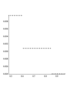
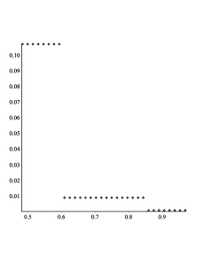
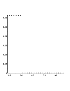
Figure 2: Computation of $v(t)$ for $k=5$ and $n=9$. In this picture we consider $\beta=1$(left), $\beta=10$(middle) and $\beta=30$(right)

In the Figure 2 we can see an approximation of the measure $\mu$ which is the only eigenmeasure of $B_{R}^{*}$ for three different values of $\beta$: $\beta=1$, $\beta=10$ and $\beta=30$. For bigger values of $\beta$ the measure is concentrated close to the smaller values of $t$. By our representation the value $t=2^{-2}a_{1}+\cdots+2^{-6}a_{5}$ corresponds to the cylinders $(\overline{1,1,1,1,1}$), $(\overline{1,1,1,1,2})$,…,$(\overline{1,1,2,2,1})$ and $(\overline{1,1,2,2,2})$.

5 The Haar Operator

We already proved that certain eigenmeasures of the Haar-Ruelle operators are quasi-invariant measures. In this section we are going to consider necessary conditions on the quasi-invariant measure. Our goal is to show that any quasi-invariant measure is an eigenmeasure of some Haar operator. We notice that this operator is quite different from the Haar-Ruelle operator.

Definition 5.1.

We introduce the Haar operator, $H_{-\beta c}$ defined by

$$H_{-\beta c}(f)(x)=\frac{1}{\nu^{x}([x])}\int_{s\in[x]}f(s)\,e^{-\beta c(x,s)}d\nu^{x}(s),$$

acting on any integrable $f:X\to\mathbb{R}$.

Proposition 5.2.

We claim that
a) $H_{-\beta c}:C^{0}\to C^{0}$.
b) $H_{-\beta c}^{2}=H_{-\beta c}$, in particular $V=H_{-\beta c}(f)$ for a given $f:X\to\mathbb{R}$ is a fixed point, that is, $H_{-\beta c}(V)=V$.
c) $H_{-\beta c}$ is positive.
d) $H_{-\beta c+b}(1)=1$, for $b(x,y)=V(y)-V(x)$, where $V=\ln H_{-\beta c}(f)$, for some $f:X\to\mathbb{R}^{+}$.

Proof. a) $H_{-\beta c}:C^{0}\to C^{0}$ because the map

$$x\to[x]:=\{s\in X|s\sim x\}$$

is continuous as a set function.

b) Let $V=H_{-\beta c}(f)$ for some $f:X\to\mathbb{R}$, then,

$$H_{-\beta c}(V)(x)=\frac{1}{\nu^{x}([x])}\int_{s\in[x]}V(s)\,e^{-\beta c(x,s)}d\nu^{x}(s)=$$

$$=\frac{1}{\nu^{x}([x])}\int_{s\in[x]}\frac{1}{\nu^{s}([s])}\int_{t\in[s]}f(t)\,e^{-\beta c(s,t)}d\nu^{s}(t)\,e^{-\beta c(x,s)}d\nu^{x}(s)=$$

$$=\frac{1}{\nu^{x}([x])}\int_{t\in[x]}f(t)\,e^{-\beta c(x,t)}d\nu^{x}(t)=V(x),$$

because $c(x,t)=c(x,s)+c(s,t),\forall x\sim s\sim t$.

c) It is obvious.

d) Consider $V=\ln H_{-\beta c}(f)$, for any $f:X\to\mathbb{R}^{+}$, and $b(x,y)=V(y)-V(x)$, then,

$$H_{-\beta c+b}(1)=\frac{1}{\nu^{x}([x])}\int_{s\in[x]}1\,e^{-\beta c(x,s)+b(x,s)}d\nu^{x}(s)=$$

$$=\frac{1}{\nu^{x}([x])}\int_{s\in[x]}1\,e^{-\beta c(x,s)+V(s)-V(x)}d\nu^{x}(s)=$$

$$=\frac{e^{-V(x)}}{\nu^{x}([x])}\int_{s\in[x]}e^{V(s)}\,e^{-\beta c(x,s)}d\nu^{x}(s)=\frac{H_{-\beta c}(e^{V})(x)}{e^{V(x)}}=1,$$

because $H_{-\beta c}(e^{V})=e^{V}$. $\blacksquare$

From the previous result we can establish a standard normalization. Since $H_{-\beta c}(1)(x)>0$ we have that $V(x)=\ln H_{-\beta c}(1)(x)$ and

$$H_{-\beta c+b}(f)(x)=\frac{1}{\nu^{x}([x])}\int_{s\in[x]}f(s)\,e^{-\beta c(x,s)+\ln H_{-\beta c}(1)(s)-\ln H_{-\beta c}(1)(x)}d\nu^{x}(s)$$

satisfies $H_{-\beta c+b}(1)=1$, where

$$V(x)=\ln H_{-\beta c}(1)(x)=\frac{1}{\nu^{x}([x])}\int_{s\in[x]}e^{-\beta c(x,s)}d\nu^{x}(s).$$

This kind of normalization is analogous, in some sense, to the one presented in [16] or in [14].

6 Characterizing quasi-invariant probabilities

Suppose that $M$ is a quasi-invariant probability for $\beta\in\mathbb{R}$ and $c:G\rightarrow\mathbb{R}$, that is, for any $h$

$$\int\int h(s,\ x)d\nu^{x}(s)dM(x)=\int\int h(x,\ s)e^{-\beta c(x,s)}d\nu^{x}(s)dM(x).$$

Since $M$ is a probability in $G^{0}$, it will be completely determined by its action on $C^{0}$.

Proposition 6.1.

If $M$ is a quasi-invariant probability for $\beta\in\mathbb{R}$ and $c:G\rightarrow\mathbb{R}$, then

$$\int_{G^{0}}f(x)dM(x)=\int_{G^{0}}H_{-\beta c}(f)(x)dM(x),$$

for all $f\in C^{0}$.

Proof. Consider $f\in C^{0}$ and define the integrable function

$$h(x,y)=\frac{f(s)}{\nu^{x}([x])},$$

then,

$$\int_{G^{0}}\int_{[x]}\frac{f(x)}{\nu^{s}([s])}d\nu^{x}(s)dM(x)=\int_{G^{0}}\int_{[x]}\frac{f(s)}{\nu^{x}([x])}e^{-\beta c(x,s)}d\nu^{x}(s)dM(x)$$

$$\int_{G^{0}}f(x)dM(x)=\int_{G^{0}}\frac{1}{\nu^{x}([x])}\int_{[x]}f(s)e^{-\beta c(x,s)}d\nu^{x}(s)dM(x)$$

$\blacksquare$

Proposition 6.2.

Consider $V(x)=\ln H_{-\beta c}(1)(x)$ and the normalization

$$H_{-\beta c+b}(f)(x)=\frac{1}{\nu^{x}([x])}\int_{s\in[x]}f(s)\,e^{-\beta c(x,s)+V(s)-V(x)}d\nu^{x}(s),$$

where $\displaystyle V(x)=\ln H_{-\beta c}(1)(x)=\frac{1}{\nu^{x}([x])}\int_{s\in[x]}e^{-\beta c(x,s)}d\nu^{x}(s).$ Then, $e^{V}dM=dM^{*}$ is an eigenmeasure of $H_{-\beta c+b}^{*}$. Reciprocally, if $H_{-\beta c+b}^{*}(M^{*})=M^{*}$, then $dM=e^{-V}dM^{*}$ satisfies

$$\int_{G^{0}}f(x)dM(x)=\int_{G^{0}}H_{-\beta c}(f)(x)dM(x),$$

for all $f\in C^{0}$.

Proof. Given $e^{V}dM=dM^{*}$ and $f\in C^{0}$, we define $g=fe^{V}$, then

$$\int_{G^{0}}g(x)dM(x)=\int_{G^{0}}H_{-\beta c}(g)(x)dM(x)$$

$$\int_{G^{0}}f(x)e^{V(x)}dM(x)=\int_{G^{0}}H_{-\beta c}(fe^{V})(x)dM(x)$$

$$\int_{G^{0}}f(x)dM^{*}(x)=\int_{G^{0}}H_{-\beta c}(fe^{V})(x)e^{-V(x)}e^{V(x)}dM(x)$$

$$\int_{G^{0}}f(x)dM^{*}(x)=\int_{G^{0}}\frac{1}{\nu^{x}([x])}\int_{[x]}f(s)e^{V(s)}e^{-\beta c(x,s)}\nu^{x}(ds)e^{-V(x)}dM^{*}(x)$$

$$\int_{G^{0}}f(x)dM^{*}(x)=\int_{G^{0}}H_{-\beta c+b}(f)(x)dM^{*}(x).$$

The reciprocal is true because we can reverse the previous argument. $\blacksquare$

A. O. Lopes

arturoscar.lopes@gmail.com

partially supported by CNPq

E. R. Oliveira

elismar.oliveira@ufrgs.br

Instituto de Matematica e Estatistica - UFRGS

References

• [1] Charalambos D. Aliprantis and Kim C. Border. Infinite dimensional analysis. Springer, Berlin, third edition, 2006. A hitchhiker’s guide.
• [2] A. T. Baraviera, L. M. Cioletti, A. O. Lopes, Joana Mohr and Rafael R. Souza, On the general one-dimensional $XY$ model: positive and zero temperature, selection and non-selection. Rev. Math. Phys., 23(10):1063–1113, 2011.
• [3] G. Castro, A. O. Lopes and G. Mantovani, Haar systems, KMS states on von Neumann algebras and $C^{*}$-algebras on dynamically defined groupoids and Noncommutative Integration, preprint 2017
• [4] L. Cioletti and A. O. Lopes, Interactions, Specifications, DLR probabilities and the Ruelle Operator in the One-Dimensional Lattice, Discrete and Cont. Dyn. Syst. - Series A, Vol 37, Number 12, 6139 – 6152 (2017)
• [5] L. Cioletti and A. O. Lopes, Spectral Triples on Thermodynamic Formalism and Dixmier trace representations of Gibbs measures, preprint arXiv (2018)
• [6] L. Cioletti and E. R. Oliveira, Thermodynamic Formalism for Iterated Function Systems with Weights, preprint Arxiv (2017)
• [7] A. Connes, Sur la theorie non commutative de l’integration, preprint
• [8] R. Exel and A. Lopes, $C^{*}$-Algebras, Approximately Proper Equivalence Relations, and Thermodynamic Formalism, Ergodic Theo and Dyn. Syst., Vol 24, pp 1051-1082, Erg Theo and Dyn Syst (2004).
• [9] R. Exel and A. Lopes, $C^{*}$- Algebras and Thermodynamic Formalism, Sao Paulo Journal of Mathematical Sciences 2, 1 (2008), 285–-307
• [10] A. H. Fan and Ka-Sing Lau, Iterated function system and Ruelle operator. J. Math. Anal. Appl., 231(2):319–344, 1999.
• [11] A. Kumjian and J. Renault, KMS states on $C^{*}$-Algebras associated to expansive maps, Proc. AMS Vol. 134, No. 7, 2067-2078 (2006)
• [12] A. O. Lopes and G. Mantovani, The KMS Condition for the homoclinic equivalence relation and Gibbs probabilities, preprint Arxiv 2017
• [13] A. O. Lopes and E. R. Oliveira, Entropy and variational principles for holonomic probabilities of IFS. Discrete Contin. Dyn. Syst., 23(3):937–955, 2009.
• [14] A. O. Lopes, J. K. Mengue, J. Mohr and R. R. Souza, Entropy and Variational Principle for one-dimensional Lattice Systems with a general a-priori probability: positive and zero temperature, Erg. Theory and Dyn Systems, 35 (6), 1925–-1961 2015
• [15] J. Mengue and E. R. Oliveira, Duality results for iterated function systems with a general family of branches, Stoch. Dyn. 17 (2017), no. 3, 1750021, 23 pp
• [16] W. Parry and M. Pollicott. Zeta functions and the periodic orbit structure of hyperbolic dynamics. Astérisque, (187-188):268, 1990.
• [17] J. Renault, $C^{*}$-Algebras and Dynamical Systems, XXVII Coloquio Bras. de Matematica - IMPA (2009)