Decoupling of charm beyond leading order

Abstract

We study the effective theory of decoupling of a charm quark at low energies. We do this by simulating a model, QCD with two mass-degenerate charm quarks. At leading order the effective theory is a pure gauge theory. By computing ratios of hadronic scales we have direct access to the power corrections in the effective theory. We show that these corrections follow the expected leading behavior, which is quadratic in the inverse charm quark mass.

1 Introduction

Several lattice groups are performing simulations of QCD₃ with up, down and strange quarks. They are cheaper and simpler than simulations of QCD₄ which includes a dynamical charm quark. The motivation to neglect the charm quark at low energies $E\ll M_{\rm charm}\equiv M_{\rm c}$ is decoupling. QCD₄ can be described by an effective theory which at leading order is QCD₃ without the charm quark. Neglecting the light quark masses, the effects of decoupling of the charm at low energies are incorporated in the matching of the gauge couplings and in the power corrections stemming from higher order terms in the effective theory. Matching of the gauge couplings of QCD₄ and QCD₃ can be performed in perturbation theory. This is used in the determination of $\alpha_{s}$ from QCD₃ simulations by the ALPHA collaboration tomaszlat17 ; Bruno:2017gxd . Non-perturbative tests of decoupling are important. On one hand to confirm the applicability of perturbation theory, on the other hand to know the size of the power corrections and whether they can be neglected. We address the latter issue here.

In order to avoid a multi-scale problem and control the continuum limit we study a model, QCD₂ with $N_{\mathrm{f}}=2$ degenerate quarks of mass $M$. In this case the effective theory for $E\ll M$ is a Yang–Mills theory ($N_{\mathrm{f}}=0$, $M=\infty$) at leading order. Beyond leading order there are power corrections starting at $M^{-2}$. In a previous work Bruno:2014ufa simulation of masses up to $M\approx M_{\rm c}/2$ allowed to estimate that the size of the power corrections is at the permille level for $M=M_{\rm c}$. These estimates were based on interpolations with the pure gauge theory at $M=\infty$. However a behaviour of the power corrections $\propto M^{-2}$ was not seen. In this contribution, which is based on Knechtli:2017xgy , we extend the mass range of the simulations to $M\gtrsim M_{\rm c}$ thus allowing a direct determination of the power corrections for a charm quark and a more stringent test of the behavior expected from the effective theory.

2 Effective theory of decoupling

In this work we consider only virtual effects of a heavy quark with mass $M$. We exclude states with explicit heavy quarks from the discussion. The decoupling of the heavy quark at low energies can be described in terms of an effective Lagrangian Weinberg:1980wa . In the case of decoupling of $N_{\mathrm{f}}=2$ mass-degenerate heavy quarks it reads

$${\mathcal{L}}_{\rm{dec}} = {\mathcal{L}}_{\rm{YM}}+\frac{1}{M^{2}}{\mathcal{L}}_{\rm{6}}+{\rm O}\left(\frac{\Lambda^{4}}{M^{4}}\right)\,,$$ (1)

$${\mathcal{L}}_{\rm{6}} = \omega_{1}\,\mathrm{tr}\{D_{\mu}F_{\nu\rho}D_{\mu}F_{\nu\rho}\}+\omega_{2}\,\mathrm{tr}\{D_{\mu}F_{\mu\rho}D_{\nu}F_{\nu\rho}\}\,.$$ (2)

In eq. (1) ${\mathcal{L}}_{\rm{YM}}$ is the Yang–Mills Lagrangian which describes the leading order in an expansion in inverse powers of $M$. Due to gauge invariance there are no dimension 5 operators. Therefore the first correction starts at $M^{-2}$ with the dimension 6 Lagrangian ${\mathcal{L}}_{\rm{6}}$ defined in eq. (2) which contains two independent terms Cho:1994yu ; Manohar:1997qy .

The Yang–Mills Lagrangian ${\mathcal{L}}_{\rm{YM}}$ has one free parameter, the gauge coupling. Matching the $N_{\mathrm{f}}=2$ and Yang–Mills theories means specifying a value of the Yang–Mills coupling at some scale or equivalently its $\Lambda$ parameter. Matching can be described by the relation

$$\Lambda_{\rm YM}(M,\Lambda)=P(M/\Lambda)\,\Lambda$$ (3)

which expresses the effective Lambda parameter $\Lambda_{\rm YM}$ of the Yang–Mills theory after matching as a function of the heavy quark mass and the Lambda parameter of the $N_{\mathrm{f}}=2$ theory $\Lambda\equiv\Lambda^{(N_{\mathrm{f}}=2)}$. For dimensional reasons this function is a dimensionless factor $P(M/\Lambda)$ times $\Lambda$.

Consider a low energy hadronic observable $m^{\mathrm{had}}$. It can be a hadronic scale such as $1/\sqrt{t_{0}}$ Luscher:2010iy or $1/r_{0}$ Sommer:1993ce . After matching it takes the same value in both theories up to power corrections:

$$m^{\mathrm{had}}(M)=m^{\mathrm{had}}_{\rm YM}+{\rm O}(\Lambda^{2}/M^{2})$$ (4)

Note that the value $m^{\mathrm{had}}_{\rm YM}$ of the observable in the Yang–Mills theory depends on $M$ through the matching eq. (4). This mass dependence is described by the factor $P$ in eq. (3) since $c=m^{\mathrm{had}}_{\rm YM}/\Lambda_{\rm YM}$ is a pure number. Consider now two hadronic scales, $m^{\mathrm{had,1}}(M)$ and $m^{\mathrm{had,2}}(M)$, whose values in the Yang–Mills theory are denoted by $m_{\rm YM}^{\mathrm{had,1}}$ and $m_{\rm YM}^{\mathrm{had,2}}$ respectively. A consequence of the matching relation eq. (4) for the ratio of two hadronic scales is

$$R(M) = \frac{m^{\mathrm{had,1}}(M)}{m^{\mathrm{had,2}}(M)}=\frac{m_{\rm YM}^{\mathrm{had,1}}}{m_{\rm YM}^{\mathrm{had,2}}}+{\rm O}(\Lambda^{2}/M^{2})$$ (5)

Note that the ratio of scales in the Yang–Mills theory

$$\frac{m_{\rm YM}^{\mathrm{had,1}}}{m_{\rm YM}^{\mathrm{had,2}}} = \frac{m_{\rm YM}^{\mathrm{had,1}}/\Lambda_{\rm YM}}{m_{\rm YM}^{\mathrm{had,2}}/\Lambda_{\rm YM}}=\frac{c_{1}}{c_{2}}$$ (6)

is given by the ratio of two pure numbers and is independent of the Lambda parameter $\Lambda_{\rm YM}$ (or of the gauge coupling). The matching of the couplings is therefore irrelevant for the ratios in eq. (5). An immediate consequence of eq. (5) is

$$R(M)=R(\infty)+k\,\Lambda^{2}/M^{2}+{\rm O}(\Lambda^{4}/M^{4})\,,$$ (7)

where $k$ is a number which depends on the ratio $R$.

3 Model calculations with two heavy quarks

The data of Ref. Bruno:2014ufa were generated from simulations of $N_{\mathrm{f}}=2$ O($a$) improved Wilson quarks with plaquette gauge action. In this work we use $N_{\mathrm{f}}=2$ twisted mass Frezzotti:2000nk Wilson quarks at maximal twist with clover term Jansen:1998mx and plaquette gauge action. We simulated larger masses corresponding to $M_{\rm c}/\Lambda=4.8700$ (charm) and $M/\Lambda=5.7781$. We also simulated the pure gauge theory ($N_{\mathrm{f}}=0$, $M=\infty$). The parameters of the new simulations are summarized in Table 1. We use open boundary conditions and the publicly available openQCD simulation package algo:openQCD . More details on the simulations can be found in Ref. Knechtli:2017xgy .

Table 1: List of ensembles generated with a doublet of twisted mass Wilson quarks at maximal twist for masses $M=M_{\rm c}$ ($M_{\rm c}/\Lambda=4.8700$) and $M=1.2M_{\rm c}$ ($M/\Lambda=5.7781$). Also listed are the pure gauge ensembles ($N_{\mathrm{f}}=0$, $M=\infty$). Open (“o”) boundary conditions (BC) are used.

$\beta$	$a$ [${\rm fm}$]	A	BC	$T\times L^{3}$	$M/\Lambda_{\rm\overline{MS\kern-0.31502pt}\kern 0.31502pt}$	$t_{0}/a^{2}$	kMDU	$\tau_{\rm exp}$ [kMDU]
$5.6$	$\approx 0.042$	tm	o	$192\times 48^{3}$	4.8700	6.609(15)	2.0	0.08
				$192\times 48^{3}$	5.7781	6.181(11)	2.1	0.08
$5.7$	$\approx 0.036$	tm	o	$120\times 32^{3}$	4.8703	9.104(36)	17.2	0.14
				$192\times 48^{3}$	5.7781	8.565(31)	2.7	0.12
$5.88$	$\approx 0.028$	tm	o	$192\times 48^{3}$	4.8700	14.622(62)	23.1	0.24
				$120\times 32^{3}$	5.7781	14.916(93)	59.9	0.23
$6.0$	$\approx 0.023$	tm	o	$192\times 48^{3}$	4.8700	22.39(12)	22.4	0.36
$6.100$	$0.0778$	–	o	$120\times 32^{3}$	$\infty$	4.4329(32)	64.0	0.05
$6.340$	$0.0545$	–	o	$120\times 32^{3}$	$\infty$	9.034(29)	20.1	0.13
$6.340^{*}$	$0.0545$	–	o	$120\times 24^{3}$	$\infty$	9.002(31)	60.9	0.13
$6.672$	$0.0350$	–	o	$192\times 48^{3}$	$\infty$	21.924(81)	73.9	0.35
$6.900$	$0.0261$	–	o	$192\times 64^{3}$	$\infty$	39.41(15)	160.2	0.65

The lattice spacing for the $N_{\mathrm{f}}=2$ theory is determined from the scale $L_{1}/a$ Blossier:2012qu ; Fritzsch:2012wq . For the $N_{\mathrm{f}}=0$ theory we use the scale $r_{0}/a$. Our spatial box sizes $L$ are such that $Lm_{\mathrm{PS}}\gg 4$ and $L/\sqrt{t_{0}}\geq 8$. In the simulation marked by ^∗ we explicitley checked that finite volume effects are negligible.

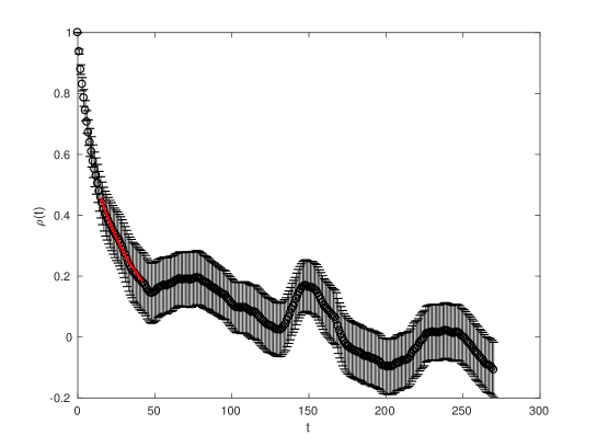
Figure 1: Autocorrelation function of $t_{0}$ for $N_{\mathrm{f}}=2$, $\beta=6.0$, $M=M_{\rm c}$. The units on the $x$-axis correspond to 16 Molecular Dynamics Units (MDU). The red line is an exponential fit to estimate the exponential autocorrelation time.

Figure 1 shows the autocorrelation function of $t_{0}$ (in units of 16 MDU) for the simulation $N_{\mathrm{f}}=2$, $\beta=6.0$, $M=M_{\rm c}$. The autocorrelation function for a derived quantity like $t_{0}$ is defined as in Eq. (33) of Ref. Wolff:2003sm . A fit of the form Schaefer:2010hu $A\exp(-t/\tau_{\rm exp})$ to the tail between $t=15$ und $t=42$ (represented by the red line in Fig. 1) gives an estimate of the exponential autocorrelation time $\tau_{\rm exp}=477(101)$ MDU. Considering all our ensembles we find a behaviour which can be parametrized by $\tau_{\rm exp}=-32(23)+17.4(2.8)\,t_{0}/a^{2}$. The scaling $\tau_{\rm exp}\propto t_{0}/a^{2}$ is expected with open boundary conditions Luscher:2011kk .

4 Results from lattice simulations

On the $N_{\mathrm{f}}=2$ and $N_{\mathrm{f}}=0$ ensembles we measure the following ratios of hadronic scales (cf. eq. (5))

$$R = \sqrt{t_{c}/t_{0}}\,,\;\sqrt{t_{0}}/w_{0}\,,\;r_{0}/\sqrt{t_{0}}\,.$$ (8)

The scale $t_{0}$ is defined through Luscher:2010iy

$${\mathcal{E}}(t_{0})=0.3\,,\quad{\mathcal{E}}(t)=t^{2}\left\langle E(x,t)\right\rangle\,.$$ (9)

where $E=\frac{1}{4}G_{\mu\nu}^{a}G_{\mu\nu}^{a}$ is the action density of the gauge field smoothed by the Wilson flow Narayanan:2006rf ; Luscher:2009eq ; Lohmayer:2011si and $t$ is the flow time whose mass dimension is $-2$. Similarly, the scale $t_{c}$ is defined by the condition

$${\mathcal{E}}(t_{c})=0.2\,.$$ (10)

The scale $w_{0}$ is defined as Borsanyi:2012zs

$$w_{0}^{2}{\mathcal{E}}^{\prime}(w_{0}^{2})=0.3\,,\quad{\cal E}^{\prime}(t)=\frac{{\rm d}}{{\rm d}t}{\cal E}(t)\,.$$ (11)

The scale $r_{0}$ is determined through the condition Sommer:1993ce

$$r_{0}^{2}F(r_{0})=1.65\,,$$ (12)

where the static force $F(r)=V^{\prime}(r)$ is the derivative of the static potential $V$.

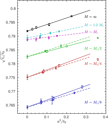
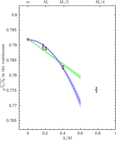
Figure 2: Left: continuum extrapolations of the ratio $R=\sqrt{t_{c}/t_{0}}$. Data are from twisted mass, standard Wilson and pure gauge simulations and are represented by pentragrams, squares and circles respectively. The lines show the fits eq. (13). Dashed lines are for twisted mass data and continued lines for Wilson and pure gauge data. The continuum extrapolated ratios are shown by the asterisks. Right: the continuum values plotted against $\Lambda/M$. The dashed line in the blue band represents the effective theory prediction eq. (7) fitted through points from $M=\infty$ down to $M/\Lambda\geq 2.5000$. The dashed line in the green band is a linear fit in $M^{-1}$.

For a given value of $M/\Lambda$ and action A (twisted mass, standard Wilson or for $M=\infty$ pure gauge) we perform continuum extrapolations of the ratios. From Symanzik’s theory we expect O($a^{2}$) cut-off effects. We fit our data to

$$R(a,M/\Lambda,{\rm A}) = R^{\rm cont}(M/\Lambda)+\frac{a^{2}}{t_{0}}c(M/\Lambda,{\rm A})\,,$$ (13)

where the fit parameters are the continuum values $R^{\rm cont}(M/\Lambda)$ and the slopes $c(M/\Lambda,{\rm A})$. In the case where simulations at the same mass were performed with two different actions we take a combined continuum limit. We apply a cut, $a^{2}/t_{0}(M)<0.32$, to the data being fitted. The fits of the ratio $R=\sqrt{t_{c}/t_{0}}$ are shown in the left plot of Fig. 2 and the continuum extrapolated values are listed in Table 2. In the right plot of Fig. 2 the continuum values $R^{\rm cont}(M/\Lambda)$ are plotted against $\Lambda/M$. The dashed line in the blue band represents the effective theory prediction eq. (7) fitted through data points from $M=\infty$ down to $M/\Lambda\geq 2.5000$. It has a good $\chi^{2}/{\rm dof}=1.75/2$. A linear fit in $M^{-1}$ is shown by the dashed line in the green band and has a far worse $\chi^{2}/{\rm dof}=9.55/2$. More fits are discussed in Ref. Knechtli:2017xgy . They clearly support the onset of the effective theory behavior eq. (7) once data for $M\gtrsim M_{\rm c}$ are included in the analysis.

For a check we also perform a global fit

$$R(a,M/\Lambda,{\rm A}) = R^{\rm cont}(M/\Lambda)+\frac{a^{2}}{8t_{0}}\left[c({\rm A})+\alpha({\rm A})\frac{M}{\Lambda}+\beta({\rm A})\frac{M^{2}}{\Lambda^{2}}\right]\,,$$ (14)

where the slopes are parametrized by the mass-independent coefficient $c({\rm A})$ and by the parameters $\alpha({\rm A})$, $\beta({\rm A})$ which model the mass dependence. The coefficient $c({\rm A})$ is the same for twisted mass and standard Wilson since these two actions are equivalent for massless quarks. The global fit of the ratio $R=\sqrt{t_{c}/t_{0}}$ is shown in the left plot of Fig. 3. It yields consistent continuum values with the non-global fit as can be seen from Table 2. In the right plot of Fig. 3 we show the continuum values with the quadratic (dashed line in the blue band) and linear (dashed line in the green band) fits in $M^{-1}$. Note that the errors of the continuum values are now correlated and this correlation is taken into account in the fits. The quadratic fit eq. (7) has a correlated $\chi^{2}/{\rm dof}=16.0/2$ and the linear fit has $\chi^{2}/{\rm dof}=7.6/2$. None of the fits work well although it seems that the quadratic fit describes better the curvature in the data.

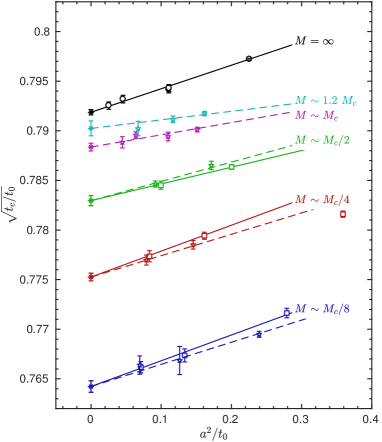
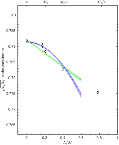
Figure 3: Left: continuum extrapolations of the ratio $R=\sqrt{t_{c}/t_{0}}$ using a global fit eq. (14). The symbols and lines are like in Fig. 2. Right: the continuum values plotted against $\Lambda/M$. The lines in the bands are like in Fig. 2. Note that the continuum data are correlated unlike in Fig. 2.

Table 2: Continuum extrapolated values of the ratios $\sqrt{t_{c}/t_{0}}$ and $\sqrt{t_{0}}/w_{0}$. The non-global extrapolations are performed using the fit eq. (13) and the global extrapolations using the fit eq. (14).

$M/\Lambda$	$\infty$	5.7781	4.87	2.50	1.28	0.59
non-global continuum limit
$\sqrt{t_{c}/t_{0}}$	0.7919(3)	0.7894(9)	0.7888(5)	0.7826(6)	0.7751(9)	0.7643(6)
$\sqrt{t_{0}}/w_{0}$	0.9803(6)	0.9774(21)	0.9765(10)	0.9661(13)	0.9532(18)	0.9311(15)
global continuum limit
$\sqrt{t_{c}/t_{0}}$	0.7919(3)	0.7902(7)	0.7884(4)	0.7830(5)	0.7753(4)	0.7642(6)
$\sqrt{t_{0}}/w_{0}$	0.9803(6)	0.9793(17)	0.9757(9)	0.9669(11)	0.9533(9)	0.9308(14)

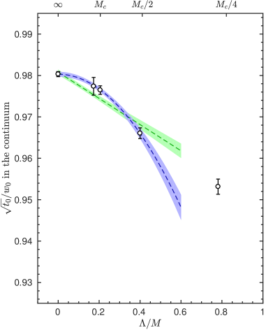
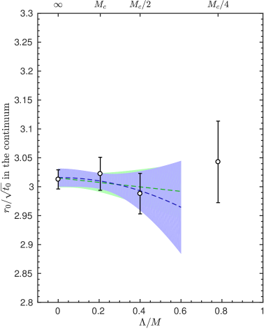
Figure 4: Left: the continuum values of the ratio $R=\sqrt{t_{0}}/w_{0}$ determined from the fit eq. (13) plotted against $\Lambda/M$. The lines in the bands are like in the right plot of Fig. 2. Right: same for the ratio $R=r_{0}/\sqrt{t_{0}}$.

The continuum extrapolated values of the ratios $R=\sqrt{t_{0}}/w_{0}$ (left plot) and $R=r_{0}/\sqrt{t_{0}}$ (right plot) are plotted against $\Lambda/M$ in Fig. 4. They are obtained using the fit eq. (13). The ratio $R=\sqrt{t_{0}}/w_{0}$ strongly favors the $M^{-2}$ behavior as it is the case for $R=\sqrt{t_{c}/t_{0}}$. Although a state of the art determination for $r_{0}$ has been used Donnellan:2010mx , the precision of the ratio $R=r_{0}/\sqrt{t_{0}}$ is not enough to resolve the power corrections.

5 Conclusions and outlook

We studied the decoupling of a charm quark non-perturbatively in QCD with two heavy quarks of mass $M$. By comparing ratios of hadronic flow scales to their values in the Yang–Mills theory we are able to measure the effects of a dynamical charm quark which are of 2 permille size. Our data can be very well fitted by the effective theory prediction for the power corrections $\propto M^{-2}$ down to masses $M_{\rm c}/2$.

As an outlook, we are computing the effects of a dynamical charm in other observables such as the charm quark mass and charmonium Korzec:2016eko and the strong coupling from the static force Cali:2017brl .

Acknowledgements. The authors gratefully acknowledge the Gauss Centre for Supercomputing (GCS) for providing computing time for a GCS Large-Scale Project on the GCS share of the supercomputer JUQUEEN at Jülich Supercomputing Centre (JSC). GCS is the alliance of the three national supercomputing centres HLRS (Universität Stuttgart), JSC (Forschungszentrum Jülich), and LRZ (Bayerische Akademie der Wissenschaften), funded by the German Federal Ministry of Education and Research (BMBF) and the German State Ministries for Research of Baden-Württemberg (MWK), Bayern (StMWFK) and Nordrhein-Westfalen (MIWF). GM acknowledges support from the Herchel Smith Fund at the University of Cambridge. This work is supported by the Deutsche Forschungsgemeinschaft in the SFB/TR 55.

References

- (1) M. Bruno, M. Dalla Brida, P. Fritzsch, T. Korzec, A. Ramos, S. Schaefer, H. Simma, S. Sint, R. Sommer (ALPHA), Determination of the Strong Coupling Constant by the ALPHA Collaboration, in Proceedings, 35th International Symposium on Lattice Field Theory (Lattice2017): Granada, Spain, to appear in EPJ Web Conf.
- (2) M. Bruno, M. Dalla Brida, P. Fritzsch, T. Korzec, A. Ramos, S. Schaefer, H. Simma, S. Sint, R. Sommer, Phys. Rev. Lett. 119, 102001 (2017), 1706.03821
- (3) M. Bruno, J. Finkenrath, F. Knechtli, B. Leder, R. Sommer (ALPHA), Phys. Rev. Lett. 114, 102001 (2015), 1410.8374
- (4) F. Knechtli, T. Korzec, B. Leder, G. Moir (2017), 1706.04982
- (5) S. Weinberg, Phys. Lett. B91, 51 (1980)
- (6) P.L. Cho, E.H. Simmons, Phys. Rev. D51, 2360 (1995), hep-ph/9408206
- (7) A.V. Manohar, Phys. Rev. D56, 230 (1997), hep-ph/9701294
- (8) M. Lüscher, JHEP 08, 071 (2010), [Erratum: JHEP03,092(2014)], 1006.4518
- (9) R. Sommer, Nucl. Phys. B411, 839 (1994), hep-lat/9310022
- (10) R. Frezzotti, P.A. Grassi, S. Sint, P. Weisz (Alpha), JHEP 08, 058 (2001), hep-lat/0101001
- (11) K. Jansen, R. Sommer (ALPHA), Nucl. Phys. B530, 185 (1998), [Erratum: Nucl. Phys.B643,517(2002)], hep-lat/9803017
- (12) M. Lüscher, S. Schaefer, Comput.Phys.Commun. 184, 519 (2013), 1206.2809
- (13) B. Blossier, M. Della Morte, P. Fritzsch, N. Garron, J. Heitger, H. Simma, R. Sommer, N. Tantalo (ALPHA), JHEP 09, 132 (2012), 1203.6516
- (14) P. Fritzsch, F. Knechtli, B. Leder, M. Marinkovic, S. Schaefer, R. Sommer, F. Virotta, Nucl. Phys. B865, 397 (2012), 1205.5380
- (15) U. Wolff (ALPHA collaboration), Comput.Phys.Commun. 156, 143 (2004), hep-lat/0306017
- (16) S. Schaefer, R. Sommer, F. Virotta (ALPHA Collaboration), Nucl.Phys. B845, 93 (2011), 1009.5228
- (17) M. Lüscher, S. Schaefer, JHEP 1107, 036 (2011), 1105.4749
- (18) R. Narayanan, H. Neuberger, JHEP 03, 064 (2006), hep-th/0601210
- (19) M. Lüscher, Commun. Math. Phys. 293, 899 (2010), 0907.5491
- (20) R. Lohmayer, H. Neuberger, PoS LATTICE2011, 249 (2011), 1110.3522
- (21) S. Borsanyi, S. Dürr, Z. Fodor, C. Hoelbling, S.D. Katz, S. Krieg, T. Kurth, L. Lellouch, T. Lippert, C. McNeile et al., JHEP 09, 010 (2012), 1203.4469
- (22) M. Donnellan, F. Knechtli, B. Leder, R. Sommer, Nucl.Phys. B849, 45 (2011), 1012.3037
- (23) T. Korzec, F. Knechtli, S. Cali, B. Leder, G. Moir, Impact of dynamical charm quarks, in Proceedings, 34th International Symposium on Lattice Field Theory (Lattice 2016): Southampton, UK, July 24-30, 2016 (2016), 1612.07634
- (24) S. Calì, F. Knechtli, T. Korzec, H. Panagopoulos, Charm quark effects on the strong coupling extracted from the static force (2017), in Proceedings, 35th International Symposium on Lattice Field Theory (Lattice2017): Granada, Spain, to appear in EPJ Web Conf., 1710.06221