Gevrey genericity of Arnold diffusion in a priori unstable Hamiltonian systems

Abstract.

It is well known that under generic $C^{r}$ smooth perturbations, the phenomenon of global instability, known as Arnold diffusion, exists in a priori unstable Hamiltonian systems. In this paper, by using variational methods, we will prove that under generic Gevrey smooth perturbations, Arnold diffusion still exists in the a priori unstable Hamiltonian systems of two and a half degrees of freedom.

1. Introduction

Throughout this paper, we denote by $\mathbb{T}^{n}\times\mathbb{R}^{n}$ the cotangent bundle $T^{*}\mathbb{T}^{n}$ of the torus $\mathbb{T}^{n}$ with $\mathbb{T}=\mathbb{R}/\mathbb{Z}$, and endow $\mathbb{T}^{n}\times\mathbb{R}^{n}$ with its usual coordinates $(q,p)$ where $q=(q_{1},\cdots,q_{n})$ and $p=(p_{1},\cdots,p_{n})$. We also endow the phase space with its canonical symplectic form $\Omega=\sum_{i=1}^{n}dq_{i}\wedge dp_{i}$. A Hamiltonian system is usually a dynamical system governed by the following Hamilton’s equations

$$\dot{q}=\frac{\partial H}{\partial p},\quad\dot{p}=-\frac{\partial H}{\partial q},\quad(q,p)\in\mathbb{T}^{n}\times\mathbb{R}^{n}$$

where $H(q,p,t)$ is a Hamiltonian function and the dependence on the time $t$ is $1$-periodic, so $t\in\mathbb{T}$.

The goal of this paper is to present global instability in a class of Hamiltonians. The problem of the influence of small perturbations on an integrable Hamiltonian system was considered by Poincaré to be the fundamental problem of Hamiltonian dynamics. It is customary to consider a nearly-integrable Hamiltonian system of the form $H=H_{0}(p)+\varepsilon H_{1}(q,p,t)$. Notice that for $\varepsilon=0$ such systems do not admit any instability phenomenon. For $0<\varepsilon\ll 1$, the celebrated KAM theory asserts that a set of nearly full measure in the phase space consists of invariant tori carrying quasi-periodic motions, and the oscillation of the action variables $p$ on each KAM torus is at most of order $\sqrt{\varepsilon}$. For $n\geq 2$, the complement of the set of the union of KAM tori is connected, so a natural question that arises is whether it is possible to find large evolution of order $1$. In the celebrated paper [1], Arnold first proposed an example of a nearly-integrable Hamiltonian system with two and a half degrees of freedom, which admits trajectories whose action variables have large oscillation. Moreover, he also conjectured that such an instability phenomenon occurs in generic nearly-integrable systems. This is known as the Arnold diffusion conjecture, and it has been investigated extensively since then.

The mechanism of Arnold’s original example is based on the existence of a normally hyperbolic invariant cylinder (NHIC) foliated by a family of hyperbolic invariant tori or whiskered tori. The unstable manifold of one torus intersects transversally the stable manifold of another nearby torus. These tori constitute a transition chain along which diffusion takes place. By Nekhoroshev theory, it must be extremely slow. This mechanism has inspired a large number of studies to the Hamiltonians possessing certain hyperbolic geometric structures. In the literature, such a system is referred to as “a priori unstable”, to be distinguished from a nearly-integrable system (i.e. “a priori stable”). There have been many works devoted to the a priori unstable systems based on Arnold’s geometric mechanism, and most of them have tried to find transition chains in more general cases [8, 9, 29, 42, 52, 60, 79], etc. However, for a general a priori unstable system the transition chain cannot be formed by a continuous family of tori but a Cantorian family, and the size of gaps between the persisting tori could be larger than the size of the intersections of the stable and unstable manifolds. This is known as the large gap problem.

In the last two decades there have been several methods to overcome the large gap problem. Among them there are mainly two methods concerning the genericity of instability: variational methods and geometric methods. The first attempt to study Arnold’s original example in variational viewpoint is by U. Bessi [10]. Essential progress has also been made by J. N. Mather. In the celebrated paper [67], he developed a powerful variational tool to study the global instability in the framework of convex Lagrangian systems. In an unpublished manuscript [68], he further showed the existence of orbits with unbounded energy in perturbations of a geodesic flow on $\mathbb{T}^{2}$ by a generic time-periodic potential. Based on Mather’s variational mechanism, the authors of [24] constructed diffusing orbits and proved the $C^{r}$-genericity ($r$ is finite and suitably large) of Arnold diffusion for the a priori unstable systems with two and a half degrees of freedom. On the other hand, several authors have used geometric methods, which also apply to Hamiltonians that are not necessarily convex, to obtain Arnold diffusion. More precisely, the authors in [32, 33, 34] defined the so-called scattering map which accounts for the outer dynamics along homoclinic orbits, and overcame the large gap problem by incorporating in the transition chain new invariant objects, like secondary tori and the stable and unstable manifolds of lower dimensional tori; In [73], the author geometrically defined the so-called separatrix map near the normally hyperbolic invariant cylinder, then he showed in [74] the existence of diffusion by making full use of the dynamics of this map, and even estimated the optimal diffusion speed of order $\varepsilon/|\log\varepsilon|$ (see also [8]). Moreover, for the case of a priori unstable Hamiltonians with higher degrees of freedom, similar results have also been obtained by variational or geometric methods in [3, 25, 36, 37, 46, 59, 75].

The a priori stable case poses a new difficulty: the presence of multiple resonances. In the paper [69] (see also [70]), Mather first made an announcement for systems with two degrees of freedom in the time-periodic case or with three degrees of freedom in the autonomous case, under a series of cusp-residual conditions. Hence the diffusion problem in this situation was thought to possess only cusp-residual genericity. The complete proof for the autonomous systems with three degrees of freedom appeared in the preprint [19], and the main ingredients have been published in the recent works [26, 22, 20, 21]. Indeed, the main difficulty in this case arises from the dynamics around strong double resonances. It is because away from double resonances, one could apply normal form theory to construct NHICs with a length independent of $\varepsilon$, along which the local instability can be obtained as in the a priori unstable case [4, 7]. To solve the problem of double resonance, the paper [20] presented a new variational mechanism to switch from one resonance to another, which eventually proved the cusp-residual genericity of diffusion in the $C^{r}$ smooth category [21]. Moreover, we mention that similar results on diffusion have also been obtained, by using variational methods, in the paper [56] and the preprint [53] for systems with 2.5 degrees of freedom. Also, we refer the reader to the preprints [62, 63, 47] for systems with 3 degrees of freedom by using the geometric tools. As for the case of arbitrarily higher degrees of freedom, we refer the reader to the preprint [23] and the announcement [54]. Anyway, there have been many other works related to the problem of Arnold diffusion but we cannot list all of them, see [11, 17, 31, 49, 43, 48, 55, 78], etc.

To the author’s knowledge, the genericity of Arnold diffusion is by now quite well understood in the $C^{r}$ smooth category, not yet in the analytic category, or the Gevrey smooth category [45]. The present paper is interested in whether the phenomenon of large evolution exists generically in the Gevrey smooth Hamiltonians. Given $\alpha\geq 1$, a Gevrey-$\alpha$ function is an ultra-differentiable function whose $k$-th order partial derivatives are bounded by $O(M^{-|k|}k!^{\alpha})$. For the case $\alpha=1$, it is exactly a real analytic function. Hence, the Gevrey class is intermediate between the $C^{\infty}$ class and the real analytic class. Besides, a key point for the Gevrey class is that it allows the existence of a function with compact support (i.e. bump function). But no analytic function has compact support.

To consider the Arnold diffusion problem in the Gevrey topology, we would adopt the Gevrey norm introduced by Marco and Sauzin in [64] during a collaboration with Herman (see Definition 1.1). Apart from the theory of PDE where it has been widely used, the Gevrey class is also studied in the field of Dynamical Systems. For example, we refer to [12, 13, 14, 15, 57, 72], etc for the stability theory, such as KAM theory and Nekhoroshev theory. We also refer the reader to [16, 58, 65, 77, 39], etc for some relevant results on instability. All these studies make us believe that one can also consider the genericity problem of diffusion in the Gevrey case.

Therefore, in this paper we start by considering the a priori unstable, Gevrey-$\alpha$ ($\alpha>1$) Hamiltonian systems of two and a half degrees of freedom. The case $\alpha=1$ (i.e. the analytic genericity) is more complicated and has not been fully studied. Here we only mention a recent work [46] which proposes a general geometric mechanism that might be useful for analytic genericity. In the same spirit as in [46], the paper [44] gives models where the analytic genericity can be achieved for a priori chaotic symplectic maps, provided that the scattering map has no monodromy and is globally defined on the NHIC.

Before stating our main results , we review the concept of Gevrey function and some standard facts.

Definition 1.1 (Gevrey function [64]).

Let $\alpha\geq 1,\mathbf{L}>0$ and $K$ be a $n$-dimensional compact domain. A real-valued $C^{\infty}$ function $f(x)$ defined on $K$ is said to be Gevrey-($\alpha,\mathbf{L}$) if

$$\|f\|_{\alpha,\mathbf{L}}:=\sum_{k\in\mathbb{N}^{n}}\frac{\mathbf{L}^{|k|\alpha}}{(k!)^{\alpha}}\|\partial^{k}f\|_{C^{0}(K)}<+\infty,$$

with the standard multi-index notation $k=(k_{1},\cdots,k_{n})\in\mathbb{N}^{n}$, $|k|=k_{1}+\cdots+k_{n}$, $k!=k_{1}!\cdots k_{n}!$ and $\partial^{k}=\partial^{k_{1}}_{x_{1}}\cdots\partial^{k_{n}}_{x_{n}}$.

Let $\mathbf{G}^{\alpha,\mathbf{L}}(K):=\{f\in C^{\infty}(K)~{}:~{}\|f\|_{\alpha,\mathbf{L}}<+\infty\}$. The space $\mathbf{G}^{\alpha,\mathbf{L}}(K)$ endowed with the norm $\|\cdot\|_{\alpha,\mathbf{L}}$ is a Banach space. Sometimes we also write $\mathbf{G}^{\alpha}(K):=\bigcup_{\mathbf{L}>0}\mathbf{G}^{\alpha,\mathbf{L}}(K)$. In particular, for $K\subset\mathbb{R}^{n}$ and $\alpha=1$, $\mathbf{G}^{1}(K)$ is exactly the space of real analytic functions on $K$: any function $f\in\mathbf{G}^{1,\mathbf{L}}(K)$ is real analytic in $K$ and admits an analytic extension in the complex domain $\{z\in\mathbb{C}^{n}:\textup{dist}(z,K)<\mathbf{L}\}$. Conversely, for any real analytic function $f$ in $K$, there exists $\mathbf{L}>0$ such that $f\in\mathbf{G}^{1,\mathbf{L}}(K)$. However, for $\alpha>1$, $\mathbf{G}^{\alpha,\mathbf{L}}(K)$ admits non-analytic functions. Therefore, the Gevrey-smooth category is intermediate between the $C^{\infty}$ category and the analytic category.

Gevrey class has the following useful properties which have been already proved in [64]:

1. The norm $\|\cdot\|_{\alpha,\mathbf{L}}$ is an algebra norm, namely $\|fg\|_{\alpha,\mathbf{L}}\leq\|f\|_{\alpha,\mathbf{L}}\|g\|_{\alpha,\mathbf{L}}$.

2. Suppose $0<\lambda<\mathbf{L}$ and $f\in\mathbf{G}^{\alpha,\mathbf{L}}(K)$, then all partial derivatives of $f$ belong to $\mathbf{G}^{\alpha,\mathbf{L}-\lambda}(K)$ and $\sum\limits_{k\in\mathbb{N}^{n},|k|=l}\|\partial^{k}f\|_{\alpha,\mathbf{L}-\lambda}\leq l!^{\alpha}\lambda^{-l\alpha}\|f\|_{\alpha,\mathbf{L}}.$

3. Let $f\in\mathbf{G}^{\alpha,\mathbf{L}}(K_{m})$ where $K_{m}$ is a $m$-dimensional domain and let $g=(g_{1},\cdots,g_{m})$ be a mapping whose component $g_{i}\in\mathbf{G}^{\alpha,\mathbf{L}_{1}}(K_{n})$ . If $g(K_{n})\subset K_{m}$ and $\|g_{i}\|_{\alpha,\mathbf{L}_{1}}-\|g_{i}\|_{C^{0}(K_{n})}\leq\mathbf{L}^{\alpha}/n^{\alpha-1}$ for all $1\leq i\leq m,$ then $f\circ g\in\mathbf{G}^{\alpha,\mathbf{L}_{1}}(K_{n})$ and $\|f\circ g\|_{\alpha,\mathbf{L}_{1}}\leq\|f\|_{\alpha,\mathbf{L}}$.

1.1. Setup and main result

The current paper will mainly focus on the convex Hamiltonians of two and a half degrees of freedom. As we will see later, all discussions will be restricted on a compact domain in $\mathbb{T}^{2}\times\mathbb{R}^{2}\times\mathbb{T}$, so we fix, once and for all, a constant $R>1$ and a compact set

$$\mathscr{D}_{R}=\mathbb{T}^{2}\times\bar{B}_{R}(0)\times\mathbb{T},$$

where $B_{R}(0)\subset\mathbb{R}^{2}$ is an open ball of radius $R$ centered at 0 and $\bar{B}_{R}(0)$ is the closure. By Definition 1.1, the space $\mathbf{G}^{\alpha,\mathbf{L}}(\mathscr{D}_{R})$ consists of all real-valued smooth functions $f(q,p,t)$ satisfying

$$\|f\|_{\alpha,\mathbf{L}}=\sum_{k\in\mathbb{N}^{5}}\frac{\mathbf{L}^{|k|\alpha}}{k!^{\alpha}}\|\partial^{k}f\|_{C^{0}(\mathscr{D}_{R})}<+\infty,$$ (1.1)

Let $C^{\omega}_{d}(\mathscr{D}_{R})$ be the space of all real-valued analytic functions on $\mathscr{D}_{R}$, admitting an analytic extension in the complex domain $\{(q,p,t)\in(\mathbb{C}/\mathbb{Z})^{2}\times\mathbb{C}^{2}\times(\mathbb{C}/\mathbb{Z}):\|\textup{Im}q\|_{\infty}<d,~{}\textup{dist}(p,\bar{B}_{R}(0))<d,|\textup{Im}t|<d\}$. Set $C^{\omega}(\mathscr{D}_{R})=\bigcup_{d>0}C^{\omega}_{d}(\mathscr{D}_{R})$, it is well known that

1. For $\alpha\geq 1$, $\mathbf{L}>0$ and any $d>\mathbf{L}^{\alpha}$,

   $$C^{\omega}_{d}(\mathscr{D}_{R})\subset\mathbf{G}^{\alpha,\mathbf{L}}(\mathscr{D}_{R})\subset C^{\infty}(\mathscr{D}_{R}),\quad C^{\omega}(\mathscr{D}_{R})\subset\mathbf{G}^{\alpha}(\mathscr{D}_{R})\subset C^{\infty}(\mathscr{D}_{R}).$$

2. $C^{\omega}(\mathscr{D}_{R})=\mathbf{G}^{1}(\mathscr{D}_{R}).$

Now, we introduce the a priori unstable Hamiltonian model considered in this paper and state the main assumptions. Let $q=(q_{1},q_{2})\in\mathbb{T}^{2}$ and $p=(p_{1},p_{2})\in\mathbb{R}^{2}$. We consider a time-periodic and $C^{r}(r>2)$ smooth Hamiltonian of the form:

$$H(q,p,t)=H_{0}(q,p)+H_{1}(q,p,t),\quad\text{where}\quad H_{0}(q,p)=h_{1}(p_{1})+h_{2}(q_{2},p_{2}).$$ (1.2)

Here, the term $H_{1}$ is a small perturbation which is periodic of period 1 in $t$. Our main assumptions on $H_{0}$ are the following:

1. Convexity and superlinearity: for each $q\in\mathbb{T}^{2}$, the Hessian $\partial_{pp}H_{0}(q,p)$ is positive definite, and $\lim_{\|p\|\rightarrow+\infty}H_{0}(q,p)/\|p\|=+\infty.$

2. A priori hyperbolicity: the Hamiltonian flow $\Phi^{t}_{h_{2}}$, determined by $h_{2}$, has a hyperbolic fixed point $(q_{2},p_{2})=(x^{*},y^{*})$. Moreover, the function $h_{2}(q_{2},y^{*}):\mathbb{T}\rightarrow\mathbb{R}$ attains its unique maximum at $q_{2}=x^{*}$. Without loss of generality, we can assume $(x^{*},y^{*})=(0,0)$.

A prototype example of such a system is the coupling of a rotator and a pendulum

$$H=\frac{p_{1}^{2}}{2}+\frac{p_{2}^{2}}{2}+(\cos 2\pi q_{2}-1)+H_{1}(q,p,t),$$

which has been considered many times in the literature. Keep this example in mind will help the reader better understand our result and method. As we will see later, the above assumptions (H1)–(H2) are in the same spirit as in [24] while our main result and approach have some differences.

Let $\mathfrak{B}^{\mathbf{L}}_{\varepsilon,R}=\{H_{1}\in C^{\infty}(\mathscr{D}_{R}):\|H_{1}\|_{\alpha,\mathbf{L}}<\varepsilon\}$ $\subset\mathbf{G}^{\alpha,\mathbf{L}}(\mathscr{D}_{R})$ denote the open ball of radius $\varepsilon$ centered at the origin with respect to the norm $\|\cdot\|_{\alpha,\mathbf{L}}$.

Theorem 1.2.

Let $\alpha>1,R>1$ and assume that $H_{0}$ in (1.2) is of class $C^{r}$ $(r>2)$, then there exists a positive constant $\mathbf{L}_{0}=\mathbf{L}_{0}(H_{0},\alpha,R)$ such that, for each $\mathbf{L}\in(0,\mathbf{L}_{0}]$ and a sequence of open balls $B_{s}(y_{1}),\cdots,B_{s}(y_{k})\subset\mathbb{R}^{2}$, of radius $s$ centered at $y_{\ell}\in[-R+1,R-1]\times\{0\}\subset\mathbb{R}^{2}$, $\ell=1,\cdots,k$, we have:

there exist a positive number $\varepsilon_{0}=\varepsilon_{0}(H_{0},\alpha,R,s,\mathbf{L})$ and an open and dense subset $\mathfrak{S}^{\mathbf{L}}_{\varepsilon_{0},R}\subset\mathfrak{B}^{\mathbf{L}}_{\varepsilon_{0},R}$ such that for each perturbation $H_{1}\in\mathfrak{S}^{\mathbf{L}}_{\varepsilon_{0},R}$, the system $H=H_{0}+H_{1}$ has a trajectory $(q(t),p(t))$ whose action variables $p(t)$ pass through the ball $B_{s}(y_{\ell})$ at the time $t=t_{\ell}$, where $t_{1}<t_{2}<\cdots<t_{k}$.

Remark.

Just as J. N. Mather did in [69, 70], the smoothness of the unperturbed Hamiltonian $H_{0}$ could differ from that of the perturbation term $H_{1}$. Notice that $\mathbf{L}_{0}$ can not be an arbitrary constant, the reason is that our approach needs to adopt the Gevrey approximation (see Theorem 5.3).

Remark (Autonomous case).

Recall that Mather’s cohomology equivalence is trivial for an autonomous system (cf. [2]). The problem is that, unlike the time-periodic case, there is no canonical global transverse section of the flow in an autonomous system. In [59], this difficulty was overcome by taking local transverse sections, which could generalize Mather’s cohomology equivalence. Thus we believe that the Gevrey genericity is still valid for the a priori unstable autonomous Hamiltonians. However, in this paper, we only consider the non-autonomous case.

The perturbation technique used in the current paper can also prove the genericity in the sense of Mañé, which means that the diffusion is still a typical phenomenon when $H_{0}$ is perturbed by potential functions. More precisely, let $\mathbf{B}^{\mathbf{L}}_{\varepsilon}$ $\subset\mathbf{G}^{\alpha,\mathbf{L}}(\mathbb{T}^{2}\times\mathbb{T})$ denote the open ball of radius $\varepsilon$ centered at the origin with respect to the norm $\|\cdot\|_{\alpha,\mathbf{L}}$, we have

Theorem 1.3.

Under the same assumptions as in Theorem 1.2, there exists $\mathbf{L}_{0}=\mathbf{L}_{0}(H_{0},\alpha,R)>0$ such that, for each $\mathbf{L}\in(0,\mathbf{L}_{0}]$ and a sequence of open balls $B_{s}(y_{1}),\cdots,B_{s}(y_{k})\subset\mathbb{R}^{2}$, of radius $s$ centered at $y_{\ell}\in[-R+1,R-1]\times\{0\}\subset\mathbb{R}^{2}$, $\ell=1,\cdots,k$, we have:

there exist a positive number $\varepsilon_{0}=\varepsilon_{0}(H_{0},\alpha,R,s,\mathbf{L})$ and an open and dense subset $\mathbf{S}^{\mathbf{L}}_{\varepsilon_{0}}\subset\mathbf{B}^{\mathbf{L}}_{\varepsilon_{0}}$ such that for each potential perturbation $H_{1}\in\mathbf{S}^{\mathbf{L}}_{\varepsilon_{0}}$, the system $H=H_{0}+H_{1}$ has a trajectory $(q(t),p(t))$ whose action variables $p(t)$ pass through the ball $B_{s}(y_{\ell})$ at the time $t=t_{\ell}$, where $t_{1}<t_{2}<\cdots<t_{k}$.

1.2. Outline of this paper

This paper mainly adopts variational methods to construct diffusing orbits, so it requires us to transform into Lagrangian formalism. We still denote by $\mathbb{T}^{2}\times\mathbb{R}^{2}$ the tangent bundle $T\mathbb{T}^{2}$, and endow $\mathbb{T}^{2}\times\mathbb{R}^{2}$ with its usual coordinates $(q,v)$. The Lagrangian $L:\mathbb{T}^{2}\times\mathbb{R}^{2}\times\mathbb{T}\rightarrow\mathbb{R}$ associated to $H$ is defined as follows:

$$L(q,v,t):=\max_{p}\{\langle p,v\rangle-H(q,p,t)\}=L_{0}(q,v)+L_{1}(q,v,t),\quad L_{0}=l_{1}(v_{1})+l_{2}(q_{2},v_{2}).$$ (1.3)

In our proofs, we will apply results in Mather theory, where the Lagrangian is required to satisfy the Tonelli conditions (see Section 2): the fiberwise Hessian is positive definite, fiberwise superlinear, and the completeness of the Euler-Lagrange flow.

In fact, without affecting our analysis, we can always reduce to the Tonelli case. For our Lagrangian $L=L_{0}+L_{1}$ in (1.3), it is clear that the unperturbed part $L_{0}$ is a Tonelli Lagrangian as a result of hypothesis (H1). Now, we turn to the small perturbation term $L_{1}$. As we will see later, only the information on a compact region is needed in our proofs, then it will not affect the study of Arnold diffusion if one modifies the perturbation function $L_{1}$ outside the compact set. For example, one can introduce a new function $\widetilde{L}_{1}$ which has compact support, and is identically equal to $L_{1}$ on a compact set $\{\|v\|_{q}\leq K\}$. In terms of this modification, we then introduce a new Lagrangian $\widetilde{L}:=L_{0}+\widetilde{L}_{1}$. Observe that the modified Lagrangian $\widetilde{L}$ satisfies the Tonelli conditions since the perturbation term $\widetilde{L}_{1}$ is small enough and has compact support. Also, it is quite clear that $\widetilde{L}$ and $L$ generate the same Euler-Lagrange flow when restricted on the compact region $\{\|v\|_{q}\leq K\}$. Such a modification is elementary, see for instance [69].

Therefore, in what follows, we can always assume, without loss of generality, that our Lagrangian (1.3) satisfies the Tonelli conditions. Then, through the Legendre transformation

$$\mathscr{L}:T^{*}\mathbb{T}^{2}\times\mathbb{T} \rightarrow T\mathbb{T}^{2}\times\mathbb{T},$$ (1.4)

$$(q,p,t) \mapsto(q,\frac{\partial H}{\partial p}(q,p,t),t),$$

we can write

$$L(q,v,t)=\langle\pi_{p}\circ\mathscr{L}^{-1}(q,v,t),v\rangle-H\circ\mathscr{L}^{-1}(q,v,t),$$

where $\pi_{p}$ denotes the projection $(q,p,t)\mapsto p$. Then, the Hamilton’s equations $\dot{q}=\frac{\partial H}{\partial p}$, $\dot{p}=-\frac{\partial H}{\partial q}$ is equivalent to the Euler-Lagrange equation

$$\frac{d}{dt}\bigg{(}\frac{\partial L}{\partial v}\bigg{)}-\frac{\partial L}{\partial q}=0.$$

Throughout this paper, we use $\phi^{t}_{L}$ to denote the Euler-Lagrange flow determined by $L$ and $\Phi^{t}_{H}$ to denote the Hamiltonian flow determined by $H$.

The Fenchel inequality and hypothesis (H2) together give rise to

$$h_{2}(q_{2},0)+l_{2}(q_{2},v_{2})\geq 0,\quad h_{2}(0,0)+l_{2}(0,0)=0,\quad(q_{2},v_{2})\in T\mathbb{T}.$$

Since $q_{2}=0$ (mod 1) is the unique maximum point of the function $h_{2}(\cdot,0):\mathbb{T}\to\mathbb{R}$, one gets

$$l_{2}(0,0)=-h_{2}(0,0)\leq-h_{2}(q_{2},0)\leq l_{2}(q_{2},v_{2}),\quad(q_{2},v_{2})\in T\mathbb{T}.$$ (1.5)

Then the point $(q_{2},v_{2})=(0,0)$ is the unique minimum point of the function $l_{2}$ as a consequence of the strict convexity. Also, $(0,0)$ is a hyperbolic fixed point for the Euler-Lagrange flow $\phi^{t}_{l_{2}}$.

Compared with the variational proofs of $C^{r}$-genericity in [24, 25], the method in this paper contains some new techniques. Indeed, the strategy used in [24, 25], which perturbs the generating functions to create genericity, seems not applicable to the Gevrey genericity. The main difficulty arises from the fact that, when we estimate the Gevrey smoothness of a Hamiltonian flow, we cannot avoid the decrease of Gevrey coefficient $\mathbf{L}$ during the switch from a generating function to its corresponding Hamiltonian, or the switch from a Lagrangian to its associated Hamiltonian (see property (G2) above). Thus in this paper, inspired by the ideas in [20], we decide to directly perturb a Hamiltonian by potential functions, one advantage of this approach is that the Lagrangian associated to the perturbed Hamiltonian $H+V(q,t)$ is exactly $L-V(q,t)$. To this end, some quantitative estimations are required, such as the Gevrey approximation and the corresponding inverse function theorem. It is also worth mentioning that one can establish the genericity not only in the usual sense but also in the sense of Mañé. Besides, we also believe that our results could be obtained by geometric tools, such as the scattering maps developed in [34, 30, 35, 36], or the separatrix maps in [74, 75, 37].

In our variational proof of genericity, the modulus of continuity of barrier functions is crucial. To implement this argument, the work [24] introduced the following parameterization technique: fixing an invariant curve $\Gamma_{0}$ on the NHIC, for any other invariant curve $\Gamma_{\sigma}$ on the NHIC, we parameterize it by $\sigma$, the area between the two curves. Then it can be shown that $\Gamma_{\sigma}$ is Hölder continuous with respect to $\sigma$ in the $C^{0}$ topology. However, by taking advantage of the tools in weak KAM theory, now we can show that this “area” parameter $\sigma$ is exactly the cohomology class (See section 6.2). This will help us simplify the proof.

The structure of this paper is as follows. In Section 2, we review some standard results, related to Arnold diffusion problem, in Mather theory. Section 3 discusses the elementary weak KAM solutions, and a special “barrier function” whose minimal points correspond to heteroclinic orbits. In Section 4, we introduce the concept of generalized transition chain and then give the variational mechanism of constructing diffusing orbits along this chain. In Section 5, we present some properties of Gevrey functions which are necessary for our proofs. Section 6 is the main part of this paper, and applies the tools exposed in previous sections to study the Gevrey smooth systems. First, we generalize the genericity of uniquely minimal measure in the Gevrey or analytic topology. Second, we obtain certain regularity of the elementary weak KAM solutions and show how to choose suitable Gevrey space. Finally, by proving total disconnectedness for the minimal sets of barrier functions, we establish the genericity of generalized transition chain along which the global instability occurs, this therefore completes the proofs of Theorem 1.2 and Theorem 1.3.

We would like to thank the anonymous referees for their insightful comments and valuable suggestions on improving our results.

2. Preliminaries: Mather theory

In this section, we recall some standard results in Mather theory which are necessary for the purpose of our study, the main references are Mather’s original papers [66, 67]. Let $M$ be a connected and compact smooth manifold without boundary, equipped with a smooth Riemannian metric $g$. Let $TM$ denote the tangent bundle, a point of $TM$ will be denoted by $(q,v)$ with $q\in M$ and $v\in T_{q}M$. We shall denote by $\|\cdot\|_{q}$ the norm induced by $g$ on the fiber $T_{q}M$. A time-periodic $C^{2}$ function $L=L(q,v,t):TM\times\mathbb{T}\rightarrow\mathbb{R}$ is called a Tonelli Lagrangian if it satisfies:

1. Convexity: $L$ is strictly convex in each fiber, i.e., the second partial derivative $\partial^{2}L/\partial v^{2}(q,v,t)$ is positive definite, as a quadratic form, for each $(q,t)\in M\times\mathbb{T}$;

2. Superlinear growth: $L$ is superlinear in each fiber, i.e. for each $(q,t)\in M\times\mathbb{T}$,

   $$\lim_{\|v\|_{q}\rightarrow+\infty}\frac{L(q,v,t)}{\|v\|_{q}}=+\infty.$$

3. Completeness: All solutions of the Euler-Lagrange equation are well defined for all $t\in\mathbb{R}$.

Let $I=[a,b]$ be an interval and $\gamma:I\rightarrow M$ be any absolutely continuous curve. Given a cohomology class $c\in H^{1}(M,\mathbb{R})$, we choose and fix a closed 1-form $\eta_{c}$ with $[\eta_{c}]=c$. Denote by

$$A_{c}(\gamma):=\int_{a}^{b}L(d\gamma(t),t)-\eta_{c}(d\gamma(t))\,dt$$

the action of $L-\eta_{c}$ along $\gamma$, where $d\gamma(t)=(\gamma(t),\dot{\gamma}(t))$. A curve $\gamma:I\rightarrow M$ is called $c$-minimal if

$$A_{c}(\gamma)=\min_{\begin{subarray}{c}\xi(a)=\gamma(a),\xi(b)=\gamma(b)\\ \xi\in C^{ac}(I,M)\end{subarray}}\int_{a}^{b}L(d\xi(t),t)-\eta_{c}(d\xi(t))\,dt,$$

where $C^{ac}(I,M)$ denotes the set of absolutely continuous curves. As is known to all, each minimal curve satisfies the Euler-Lagrange equation. A curve $\gamma:$ $\mathbb{R}$ $\rightarrow$ $M$ is called globally $c$-minimal if for any $a<b$, the curve $\gamma:[a,b]\to M$ is $c$-minimal. Therefore, we introduce the globally minimal set

$$\widetilde{\mathcal{G}}(c):=\bigcup_{\gamma}\{(d\gamma(t),t)~{}:~{}\gamma:\mathbb{R}\rightarrow M~{}\text{is ~{}}c\text{-minimal}\}.$$

Let $\phi^{t}_{L}$ be the Euler-Lagrange flow on $TM\times\mathbb{T}$, and $\mathfrak{M}$ be the space of all $\phi^{t}_{L}$-invariant probability measures on $TM\times\mathbb{T}$. To each $\mu\in\mathfrak{M}$, Mather has proved that $\int_{TM\times\mathbb{T}}\lambda\,d\mu$=0 holds for any exact 1-form $\lambda$, which yields that $\int_{TM\times\mathbb{T}}L-\eta_{c}\,d\mu=\int_{TM\times\mathbb{T}}L-\eta^{\prime}_{c}\,d\mu$ if $\eta_{c}-\eta_{c}^{\prime}$ is exact. This leads us to define Mather’s $\alpha$ function,

$$\alpha(c):=-\inf_{\mu\in\mathfrak{M}}\int_{TM\times\mathbb{T}}L-\eta_{c}\,d\mu.$$

To some extent, the value $\alpha(c)$ is a minimal average action for $L-\eta_{c}$. Mather has proved that $\alpha:H^{1}(M,\mathbb{R})\rightarrow\mathbb{R}$ is finite everywhere, convex and superlinear.

For each $\mu\in\mathfrak{M}$, the rotation vector $\rho(\mu)$ associated with $\mu$ is the unique element in $H_{1}(M,\mathbb{R})$ that satisfies

$$\langle\rho(\mu),[\eta_{c}]\rangle=\int_{TM\times\mathbb{T}}\eta_{c}\,d\mu,\quad\text{~{} for all closed 1-form~{}}\eta_{c},$$

here $\langle\cdot,\cdot\rangle$ denotes the dual pairing between homology and cohomology classes. Then, we can define Mather’s $\beta$ function as follows:

$$\beta(h):=\inf_{\mu\in\mathfrak{M},\rho(\mu)=h}\int_{TM\times\mathbb{T}}L\,d\mu.$$

This function $\beta:H_{1}(M,\mathbb{R})\rightarrow\mathbb{R}$ is also finite everywhere, convex and superlinear. In fact, $\beta$ is the Legendre-Fenchel dual of the function $\alpha$, i.e. $\beta(h)=\max_{c}\{\langle h,c\rangle-\alpha(c)\}$.

We define

$$\mathfrak{M}^{c}(L):=\left\{\mu:\int_{TM\times\mathbb{T}}L-\eta_{c}\,d\mu=-\alpha(c)\right\},~{}\mathfrak{M}_{h}(L):=\left\{\mu:\rho(\mu)=h,\int_{TM\times\mathbb{T}}L\,d\mu=\beta(h)\right\}.$$

By duality, it can be easily checked that

$$\mathfrak{M}^{c}(L)=\bigcup_{h\in\partial\alpha(c)}\mathfrak{M}_{h}(L),$$

where $\partial\alpha(c)$ is the sub-differential. For one and a half degrees of freedom systems including twist maps, Mather’s $\alpha$ function is of class $C^{1}$, then

$$\mathfrak{M}^{c}(L)=\mathfrak{M}_{h}(L),\quad d\alpha(c)=h.$$ (2.1)

We call each element $\mu\in\mathfrak{M}^{c}(L)$ a $c$-minimal measure. The Mather set of cohomology class $c$ is then defined by

$$\widetilde{\mathcal{M}}(c):=\overline{\bigcup_{\mu\in\mathfrak{M}^{c}(L)}\text{supp}\mu}.$$

To study more dynamical properties, we need to find some “larger” minimal invariant sets and discuss their topological structures. Let $t^{\prime}>t$, the action function $h^{t,t^{\prime}}_{c}:M\times M\rightarrow\mathbb{R}$ is defined by

$$h^{t,t^{\prime}}_{c}(x,x^{\prime}):=\min_{\begin{subarray}{c}\gamma(t)=x,\gamma(t^{\prime})=x^{\prime}\\ \gamma\in C^{ac}([t,t^{\prime}],M)\end{subarray}}\int_{t}^{t^{\prime}}(L-\eta_{c})(d\gamma(s),s)\,ds+\alpha(c)\cdot(t^{\prime}-t).$$

Then we define a real-valued function $\Phi_{c}:(M\times\mathbb{T})\times(M\times\mathbb{T})\rightarrow\mathbb{R}$ by

$$\Phi_{c}((x,\tau),(x^{\prime},\tau^{\prime})):=\inf_{\begin{subarray}{c}t^{\prime}>t,~{}t\equiv\tau\text{mod}~{}1\\ t^{\prime}\equiv\tau^{\prime}\text{mod}~{}1\end{subarray}}h^{t,t^{\prime}}_{c}(x,x^{\prime}).$$

and a real-valued function $h_{c}^{\infty}:(M\times\mathbb{T})\times(M\times\mathbb{T})\rightarrow\mathbb{R}$ by

$$h_{c}^{\infty}((x,\tau),(x^{\prime},\tau^{\prime}))=\liminf\limits_{\begin{subarray}{c}t\equiv\tau\text{mod}~{}1\\ t^{\prime}\equiv\tau^{\prime}\text{mod}~{}1,t^{\prime}-t\rightarrow+\infty\end{subarray}}h^{t,t^{\prime}}_{c}(x,x^{\prime})$$ (2.2)

In the literature, $h_{c}^{\infty}$ and $\Phi_{c}$ are called the Peierls barrier function and Mañé’s potential respectively.

A minimal curve $\gamma:\mathbb{R}\rightarrow M$ is called $c$-semi static if for any $t<t^{\prime}$,

$$A_{c}(\gamma|_{[t,t^{\prime}]})+\alpha(c)\cdot(t^{\prime}-t)=\Phi_{c}\big{(}~{}(\gamma(t),t\text{~{}mod~{}}1),~{}(\gamma(t^{\prime}),t^{\prime}\text{~{}mod~{}}1)~{}\big{)}.$$ (2.3)

A minimal curve $\gamma:\mathbb{R}\rightarrow M$ is called $c$-static if for any $t<t^{\prime}$,

$$A_{c}(\gamma|_{[t,t^{\prime}]})+\alpha(c)\cdot(t^{\prime}-t)=-\Phi_{c}\big{(}~{}(\gamma(t^{\prime}),t^{\prime}\text{~{}mod~{}}1),~{}(\gamma(t),t\text{~{}mod~{}}1)~{}\big{)}.$$ (2.4)

This gives the so-called Aubry set $\widetilde{\mathcal{A}}(c)$ and Mañé set $\widetilde{\mathcal{N}}(c)$ in $TM\times\mathbb{T}$:

$$\begin{split}\widetilde{\mathcal{A}}(c)=\bigcup\big{\{}(d\gamma(t),t\text{~{}mod~{}}1):~{}\gamma~{}\text{is}~{}c\text{-static}\big{\}},~{}~{}\widetilde{\mathcal{N}}(c)=\bigcup\big{\{}(d\gamma(t),t\text{~{}mod~{}}1):~{}\gamma~{}\text{is}~{}c\text{-semi static}\big{\}}.\end{split}$$

The $\alpha$-limit and $\omega$-limit sets of a $c$-minimal curve $(d\gamma(t),t)$ belong to $\widetilde{\mathcal{A}}(c)$, see for instance [2]. In addition, with the canonical projection $\pi:TM\times\mathbb{T}\rightarrow M\times\mathbb{T}$, one could define the projected Aubry set $\mathcal{A}(c)=\pi\widetilde{\mathcal{A}}(c)$, the projected Mather set $\mathcal{M}(c)=\pi\widetilde{\mathcal{M}}(c)$, the projected Mañé set $\mathcal{N}(c)=\pi\widetilde{\mathcal{N}}(c)$ and the projected globally minimal set $\mathcal{G}(c)=\pi\widetilde{\mathcal{G}}(c)$. Then the following inclusion relations hold (see [2]):

$$\widetilde{\mathcal{M}}(c)\subset\widetilde{\mathcal{A}}(c)\subset\widetilde{\mathcal{N}}(c)\subset\widetilde{\mathcal{G}}(c),\quad\mathcal{M}(c)\subset\mathcal{A}(c)\subset\mathcal{N}(c)\subset\mathcal{G}(c).$$

Next, we present some key properties of the minimal sets above, which will be fully exploited in the construction of diffusing orbits. Property (1) below is a classical result which has been proved by J. N. Mather in [66], and the proof of property (2) could be found in [2, 24].

Proposition 2.1.

For the Tonelli Lagrangian $L$, we have:

1. (Graph property) Let $\pi:TM\times\mathbb{T}\rightarrow M\times\mathbb{T}$ be the canonical projection. Then the restriction of $\pi$ to $\widetilde{\mathcal{A}}(c)$ is a bi-Lipschitz homeomorphism.

2. (Upper semi-continuity) The set-valued map $(c,L)\mapsto\widetilde{\mathcal{G}}(c,L)$ and the set-valued map $(c,L)\mapsto\widetilde{\mathcal{N}}(c,L)$ are both upper semi-continuous.

For $(x,\tau)$, $(x^{\prime},\tau^{\prime})$ $\in M\times\mathbb{T}$, we set

$$d_{c}((x,\tau),(x^{\prime},\tau^{\prime})):=h_{c}^{\infty}((x,\tau),(x^{\prime},\tau^{\prime}))+h_{c}^{\infty}((x^{\prime},\tau^{\prime}),(x,\tau)).$$

By definition (2.4), it follows that

$$h^{\infty}_{c}((x,\tau),(x,\tau))=0\Longleftrightarrow(x,\tau)\in\mathcal{A}(c),$$

and hence $d_{c}$ is a pseudo-metric on the projected Aubry set $\mathcal{A}(c)$. Two points $(x,\tau),(x^{\prime},\tau^{\prime})\in\mathcal{A}(c)$ are said to be in the same Aubry class if $d_{c}((x,\tau),(x^{\prime},\tau^{\prime}))=0$. Clearly, each Aubry class is a closed set. If only one $c$-minimal measure exists, then the Aubry class is unique and

$$\widetilde{\mathcal{A}}(c)=\widetilde{\mathcal{N}}(c).$$

To characterize the Mañé set from another point of view, we define the following function

$$B_{c}^{*}(x,\tau):=\min\limits_{\begin{subarray}{c}(x_{\ell},\tau_{\ell})\in\mathcal{A}(c)\\ \ell=1,2\end{subarray}}\{h_{c}^{\infty}((x_{1},\tau_{1}),(x,\tau))+h_{c}^{\infty}((x,\tau),(x_{2},\tau_{2}))-h_{c}^{\infty}((x_{1},\tau_{1}),(x_{2},\tau_{2}))\}.$$

Mather has proved in [69] that $\min B_{c}^{*}=0$, and the set of all minimal points is exactly $\mathcal{N}(c)$, i.e.

$$B_{c}^{*}(x,\tau)=0\Longleftrightarrow(x,\tau)\in\mathcal{N}(c).$$ (2.5)

To prove Theorem 6.1 in Section 6, it is convenient to adopt the equivalent definition of minimal measures originating from Mañé [61]. In his setting, the minimal measures are obtained through a variational principle not requiring the invariance a priori. Let $\rm C$ be the set of all continuous functions $f:TM\times\mathbb{T}\to\mathbb{R}$ having linear growth at most, i.e.

$$\|f\|_{l}:=\sup_{(v,t)}\frac{|f(q,v,t)|}{1+\|v\|_{q}}<+\infty,$$

and endow $\rm C$ with the norm $\|\cdot\|_{l}$. Let $\rm C^{*}$ be the vector space of all continuous linear functionals $\nu:\rm C\to\mathbb{R}$ provided with the weak-$*$ topology, namely,

$$\lim\limits_{k\to+\infty}\nu_{k}=\nu\Longleftrightarrow\lim\limits_{k\to+\infty}\int_{TM\times\mathbb{T}}f\,d\nu_{k}=\int_{TM\times\mathbb{T}}f\,d\nu,\quad\forall f\in\rm C.$$

For each $N\in\mathbb{Z}^{+}$ and each $N$-periodic absolutely continuous curve $\gamma:\mathbb{R}\rightarrow M$, one can define a probability measure $\mu_{\gamma}$ associated to $\gamma$ as follows:

$$\int_{TM\times\mathbb{T}}f\,d\mu_{\gamma}:=\frac{1}{N}\int_{0}^{N}f(d\gamma(t),t)\,dt,\quad\forall f\in\rm C.$$ (2.6)

Let

$$\Gamma:=\bigcup_{N\in\mathbb{Z}^{+}}\big{\{}~{}\mu_{\gamma}~{}:~{}\gamma\in C^{ac}(\mathbb{R},M)\textup{~{}is~{}}N\textup{-periodic}~{}\big{\}}\subset\rm C^{*}.$$

and let $\mathcal{H}$ be the closure of $\Gamma$ in $\rm C^{*}$. It is easily seen that the set $\mathcal{H}$ is convex.

$\mu_{\gamma}$ in $\Gamma$ has a naturally associated homology class $\rho(\mu_{\gamma})=\frac{1}{N}[\gamma]\in H_{1}(M,\mathbb{R}),$ where $[\gamma]$ denotes the homology class of $\gamma$. The map $\rho:\Gamma\rightarrow H_{1}(M,\mathbb{R})$ can extend continuously to $\rho:\mathcal{H}\rightarrow H_{1}(M,\mathbb{R})$ which is surjective. Then, Mañé introduced the following minimal measures:

$$\begin{split}\mathfrak{H}^{c}(L)&:=\bigg{\{}\mu\in\mathcal{H}~{}:~{}\int L-\eta_{c}\,d\mu=\min\limits_{\nu\in\mathcal{H}}\int L-\eta_{c}\,d\nu\bigg{\}},\\ \mathfrak{H}_{h}(L)&:=\bigg{\{}\mu\in\mathcal{H}~{}:~{}\rho(\mu)=h,\int L\,d\mu=\min\limits_{\nu\in\mathcal{H},\rho(\nu)=h}\int L\,d\nu\bigg{\}}.\end{split}$$ (2.7)

We end this section by the following equivalence property:

Proposition 2.2.

([61]) The sets $\mathfrak{M}^{c}(L)=\mathfrak{H}^{c}(L)$ and $\mathfrak{M}_{h}(L)=\mathfrak{H}_{h}(L)$.

3. Elementary weak KAM solutions and heteroclinic orbits

3.1. Weak KAM solutions

Weak KAM solution is the basic element in weak KAM theory which builds a link between Mather theory and the theory of viscosity solutions of Hamilton-Jacobi equations. Here we only recall some basic concepts and properties which help us better understand Mather theory. For more details, we refer the reader to Fathi’s book [38] for time-independent systems, and to [3, 28, 76] for time-periodic systems.

Definition 3.1.

A continuous function $u_{c}^{-}:M\times\mathbb{T}\rightarrow\mathbb{R}$ is called a backward weak KAM solution if

1. For any absolutely continuous curve $\gamma:[a,b]\to M$,

   $$u_{c}^{-}(\gamma(b),b)-u_{c}^{-}(\gamma(a),a)\leq\int_{a}^{b}(L-\eta_{c})(d\gamma(s),s)+\alpha(c)\,ds.$$

2. For each $(x,t)\in M\times\mathbb{R}$, there exists a backward calibrated curve $\gamma^{-}:(-\infty,t]\rightarrow M$ with $\gamma^{-}(t)=x$ such that for all $a<b\leq t$,

   $$u_{c}^{-}(\gamma^{-}(b),b)-u_{c}^{-}(\gamma^{-}(a),a)=\int_{a}^{b}(L-\eta_{c})(d\gamma^{-}(s),s)+\alpha(c)\,ds.$$

Similarly, a continuous function $u_{c}^{+}:M\times\mathbb{T}\rightarrow\mathbb{R}$ is called a forward weak KAM solution if

1. For any absolutely continuous curve $\gamma:[a,b]\to M$,

   $$u_{c}^{+}(\gamma(b),b)-u_{c}^{+}(\gamma(a),a)\leq\int_{a}^{b}(L-\eta_{c})(d\gamma(s),s)+\alpha(c)\,ds.$$

2. For each $(x,t)\in M\times\mathbb{R}$, there exists a forward calibrated curve $\gamma^{+}:[t,+\infty)\rightarrow M$ with $\gamma^{+}(t)=x$ such that for all $t\leq a<b$,

   $$u_{c}^{+}(\gamma^{+}(b),b)-u_{c}^{+}(\gamma^{+}(a),a)=\int_{a}^{b}(L-\eta_{c})(d\gamma^{+}(s),s)+\alpha(c)\,ds.$$

For example, it is well known in weak KAM theory that, for each $(x_{0},t_{0})\in M\times\mathbb{T}$ the barrier function $h_{c}^{\infty}((x_{0},t_{0}),\cdot):M\times\mathbb{T}\to\mathbb{R}$ is a backward weak KAM solution and $-h_{c}^{\infty}(\cdot,(x_{0},t_{0})):M\times\mathbb{T}\to\mathbb{R}$ is a forward weak KAM solution. If there is only one Aubry class, then $h_{c}^{\infty}((x_{0},t_{0}),\cdot)$ is the unique backward weak KAM solution up to an additive constant, and $-h_{c}^{\infty}(\cdot,(x_{0},t_{0}))$ is also the unique forward weak KAM solution up to an additive constant.

It is easily seen that backward (forward) calibrated curves are semi static. The following properties for weak KAM solutions are well known and the proof can be found in [38] or [28]:

Proposition 3.2.

(1) $u^{-}_{c}$ is Lipschitz continuous, and is differentiable on $\mathcal{A}(c)$. If $u^{-}_{c}$ is differentiable at $(x_{0},t_{0})\in M\times\mathbb{T}$, then

$$\partial_{t}u^{-}_{c}(x_{0},t_{0})+H(x_{0},c+\partial_{x}u^{-}_{c}(x_{0},t_{0}),t_{0})=\alpha(c).$$

It also determines a unique $c$-semi static curve $\gamma^{-}_{c}:(-\infty,t_{0}]\rightarrow M$ with $\gamma^{-}_{c}(t_{0})=x_{0}$, and such that $u_{c}^{-}$ is differentiable at each point $(\gamma^{-}_{c}(t),t)$ with $t\leq t_{0}$, namely $c+\partial_{x}u^{-}_{c}(\gamma^{-}_{c}(t),t)=\frac{\partial L}{\partial v}(d\gamma^{-}_{c}(t),t)$.
(2) $u^{+}_{c}$ is Lipschitz continuous, and is differentiable on $\mathcal{A}(c)$. If $u^{+}_{c}$ is differentiable at $(x_{0},t_{0})\in M\times\mathbb{T}$, then

$$\partial_{t}u^{+}_{c}(x_{0},t_{0})+H(x_{0},c+\partial_{x}u^{+}_{c}(x_{0},t_{0}),t_{0})=\alpha(c).$$

It also determines a unique $c$-semi static curve $\gamma^{+}_{c}:[t_{0},+\infty)\rightarrow M$ with $\gamma^{+}_{c}(t_{0})=x_{0}$, and such that $u_{c}^{+}$ is differentiable at each point $(\gamma^{+}_{c}(t),t)$ with $t\geq t_{0}$, namely $c+\partial_{x}u^{+}_{c}(\gamma^{+}_{c}(t),t)=\frac{\partial L}{\partial v}(d\gamma^{+}_{c}(t),t)$.

3.2. Elementary weak KAM solutions

It is a generic property that a Lagrangian has finitely many Aubry classes [6] for each cohomology class. Recall that the weak KAM solution is unique (up to an additive constant) if the Aubry class is unique. If two or more Aubry classes exist, there are infinitely many weak KAM solutions, among which we are only interested in the elementary weak KAM solutions. In what follows, we assume that for certain cohomology class $c$ the Aubry classes are $\{\mathcal{A}_{c,i}:i=1,2,\cdots,k\}$, and hence the projected Aubry set $\mathcal{A}(c)=\bigcup_{i}\mathcal{A}_{c,i}.$ The concept of elementary weak KAM solution appeared in the work [3]. However, for the purpose of our applications, we decide to adopt an analogous concept defined in [19].

Definition 3.3.

We fix an $i\in\{1,\cdots,k\}$ and perturb the Lagrangian $L\rightarrow L+\varepsilon V(x,t)$ where $\varepsilon>0$ and $V$ is a non-negative $C^{\infty}$ function satisfying $\textup{supp}V\cap\mathcal{A}_{c,i}=\emptyset$ and $V\big{|}_{\mathcal{A}_{c,j}}>0$ for each $j\neq i$. Then for the cohomology class $c$, the perturbed Lagrangian has only one Aubry class $\mathcal{A}_{c,i}$, and its backward weak KAM solution, denoted by $u^{-}_{c,i,\varepsilon}$, is unique up to an additive constant. If for a subsequence $\{u^{-}_{c,i,\varepsilon_{k}}\}$, the limit

$$u^{-}_{c,i}:=\lim\limits_{\varepsilon_{k}\rightarrow 0^{+}}u^{-}_{c,i,\varepsilon_{k}},$$ (3.1)

exists, then we call $u^{-}_{c,i}$ a backward elementary weak KAM solution. Analogously, one can define a forward elementary weak KAM solution $u^{+}_{c,i}$.

In the following theorem, we will prove the existence of elementary weak KAM solutions and give explicit representation formulas as well.

Theorem 3.4.

For each $i$, the backward (resp. forward) elementary weak KAM solution $u^{-}_{c,i}$ (resp. $u^{+}_{c,i}$) always exists and is unique up to an additive constant. More precisely, let $(x_{i},\tau_{i})$ be any point in $\mathcal{A}_{c,i}$, then there exists a constant $C$ (resp. $C^{\prime}$) depending on $(x_{i},\tau_{i})$, such that

$$u^{-}_{c,i}(x,\tau)=h^{\infty}_{c}((x_{i},\tau_{i}),(x,\tau))+C\qquad(resp.~{}u^{+}_{c,i}(x,\tau)=-h^{\infty}_{c}((x,\tau),(x_{i},\tau_{i}))+C^{\prime}.)$$

Proof.

We only give the proof for $u^{-}_{c,i}$ since $u^{+}_{c,i}$ is similar. Denote by $\alpha(c)$ and $\alpha_{\varepsilon}(c)$ the value of Mather’s $\alpha$-function at the cohomology class $c$ for the Lagrangians $L-\eta_{c}$ and $L-\eta_{c}+\varepsilon V$ respectively, and denote by $h^{\infty}_{c}((x_{i},\tau_{i}),(x,\tau))$ and $h^{\infty}_{c,\varepsilon}((x_{i},\tau_{i}),(x,\tau))$ the corresponding Peierls barrier functions. We first claim that

$$h^{\infty}_{c}((x_{i},\tau_{i}),(x,\tau))=\lim\limits_{\varepsilon\to 0}h^{\infty}_{c,\varepsilon}((x_{i},\tau_{i}),(x,\tau)).$$ (3.2)

Indeed, as $V\geq 0$ and its support does not intersect with $\mathcal{A}_{c,i}$, we have $\alpha_{\varepsilon}(c)=\alpha(c)$ and

$$h^{\infty}_{c}((x_{i},\tau_{i}),(x,\tau))\leq\liminf\limits_{\varepsilon\to 0}h^{\infty}_{c,\varepsilon}((x_{i},\tau_{i}),(x,\tau)).$$

Now we turn to the opposite inequality $\limsup_{\varepsilon\to 0}h^{\infty}_{c,\varepsilon}((x_{i},\tau_{i}),(x,\tau))\leq h^{\infty}_{c}((x_{i},\tau_{i}),(x,\tau))$. Assume by contradiction that there exist a subsequence $\{h^{\infty}_{c,\varepsilon_{k}}\}_{k\in\mathbb{N}}$ and a point $(x^{\prime},\tau^{\prime})$ such that

$$\lim_{k\to\infty}h^{\infty}_{c,\varepsilon_{k}}((x_{i},\tau_{i}),(x^{\prime},\tau^{\prime}))>h^{\infty}_{c}((x_{i},\tau_{i}),(x^{\prime},\tau^{\prime}))$$ (3.3)

For abbreviation, we denote

$$\phi^{-}_{c,\varepsilon_{k}}(x,\tau):=h^{\infty}_{c,\varepsilon_{k}}((x_{i},\tau_{i}),(x,\tau)).$$ (3.4)

By Definition 3.3, $\mathcal{A}_{c,i}$ is the only Aubry class for the Lagrangian $L-\eta_{c}+\varepsilon_{k}V$, which gives $\phi^{-}_{c,\varepsilon_{k}}(x_{i},\tau_{i})$ $=0$. Moreover, it is not hard to verify that the sequence $\{\phi^{-}_{c,\varepsilon_{k}}\}_{k}$ is uniformly Lipschitz. Hence this sequence is also uniformly bounded. Thus, it follows from the Arzelà-Ascoli theorem that, by taking a subsequence if necessary, $\phi^{-}_{c,\varepsilon_{k}}$ converges uniformly to a Lipschitz function $\phi^{-}_{c}$.

It is well known in weak KAM theory that $\phi^{-}_{c}$ is a backward weak KAM solution for $L-\eta_{c}$, then

$$\phi^{-}_{c}(x,\tau)=\phi^{-}_{c}(x,\tau)-\phi^{-}_{c}(x_{i},\tau_{i})\leq h^{\infty}_{c}((x_{i},\tau_{i}),(x,\tau)),$$

further, by letting $k\to\infty$ on both sides of (3.4), we get

$$\lim_{k}h^{\infty}_{c,\varepsilon_{k}}((x_{i},\tau_{i}),(x,\tau))=\lim_{k}\phi^{-}_{c,\varepsilon_{k}}(x,\tau)=\phi^{-}_{c}(x,\tau)\leq h^{\infty}_{c}((x_{i},\tau_{i}),(x,\tau)),$$

which contradicts (3.3). This therefore proves equality $\eqref{limit of barrierfun}$.

Finally, we recall that $\mathcal{A}_{c,i}$ is the unique Aubry class for $L-\eta_{c}+\varepsilon V$ ($\varepsilon>0$). Then for any backward weak KAM solution $u^{-}_{c,i,\varepsilon}$, one has $u^{-}_{c,i,\varepsilon}(\cdot)=h^{\infty}_{c,\varepsilon}((x_{i},\tau_{i}),\cdot)+C$ with $C$ a constant. Now the theorem is evident from what we have proved. ∎

Remark.

By fixing a point $(x_{i},\tau_{i})\in\mathcal{A}_{c,i}$ for each index $i\in\{1,\cdots,k\}$, we conclude from Theorem 3.4 that the set of all backward elementary weak KAM solutions is exactly $\big{\{}h^{\infty}_{c}((x_{i},\tau_{i}),\cdot)+C~{}:~{}C\in\mathbb{R},~{}i=1,\cdots,k\big{\}}$, and the set of all forward elementary weak KAM solutions is exactly $\big{\{}-h^{\infty}_{c}(\cdot,(x_{i},\tau_{i}))+C~{}:~{}C\in\mathbb{R},~{}i=1,\cdots,k\big{\}}$.

3.3. Heteroclinic orbits between Aubry classes

To study the heteroclinic trajectories from a variational viewpoint, we will use a special type of barrier function. Indeed, let $u^{-}_{c,i}(x,\tau)$ and $u^{+}_{c,j}(x,\tau)$ be a backward and a forward elementary weak KAM solution respectively. Now we define a function

$$B_{c,i,j}(x,\tau):=u^{-}_{c,i}(x,\tau)-u^{+}_{c,j}(x,\tau),~{}\textup{for each~{}}(x,\tau)\in M\times\mathbb{T}.$$ (3.5)

Roughly speaking, it measures the action along curves joining the Aubry class $\mathcal{A}_{c,i}$ to $\mathcal{A}_{c,j}$, we refer the reader to [3, 25, 19] for more discussions.

In the sequel, the notation $\arg\min f$ denotes the minimal set $\{a~{}|~{}f(a)=\min f\}$, then we have

Proposition 3.5.

Suppose that the projected Aubry set $\mathcal{A}(c)=\bigcup_{i=1}^{k}\mathcal{A}_{c,i}$ consists of $k$ $(k\geq 2)$ Aubry classes, then the projected Mañé set

$$\mathcal{N}(c)=\bigcup_{i,j=1}^{k}\arg\min B_{c,i,j},$$

Proof.

We first prove $\mathcal{N}(c)\supseteq\arg\min B_{c,i,j}$ for each $i,j$. Taking two points $(x_{i},\tau_{i})\in\mathcal{A}_{c,i}$ and $(x_{j},\tau_{j})\in\mathcal{A}_{c,j}$, Theorem 3.4 implies that there exist two constants $C_{i}$ and $C_{j}$ such that

$$u^{-}_{c,i}(x,\tau)=h^{\infty}_{c}((x_{i},\tau_{i}),(x,\tau))+C_{i},\quad u^{+}_{c,j}(x,\tau)=-h^{\infty}_{c}((x,\tau),(x_{j},\tau_{j}))+C_{j}.$$

Thus it’s easy to compute that

$$\min B_{c,i,j}(x,\tau)=h^{\infty}_{c}((x_{i},\tau_{i}),(x_{j},\tau_{j}))+C_{i}-C_{j}.$$

If $(\tilde{x},\tilde{\tau})\in\arg\min B_{c,i,j}$, then

$$h^{\infty}_{c}((x_{i},\tau_{i}),(\tilde{x},\tilde{\tau}))+C_{i}+h^{\infty}_{c}((\tilde{x},\tilde{\tau}),(x_{j},\tau_{j}))-C_{j}=h^{\infty}_{c}((x_{i},\tau_{i}),(x_{j},\tau_{j}))+C_{i}-C_{j},$$

namely $h^{\infty}_{c}((x_{i},\tau_{i}),(\tilde{x},\tilde{\tau}))+h^{\infty}_{c}((\tilde{x},\tilde{\tau}),(x_{j},\tau_{j}))-h^{\infty}_{c}((x_{i},\tau_{i}),(x_{j},\tau_{j}))=0$. By (2.5) one obtains $(\tilde{x},\tilde{\tau})\in\mathcal{N}(c)$.

Now it remains to show $\mathcal{N}(c)\subset\bigcup_{i,j=1}^{k}\arg\min B_{c,i,j}$. For each $(\bar{x},\bar{\tau})\in\mathcal{N}(c)$, one deduces from (2.5) that there always exist $m,n\in\{1,2,\cdots,k\}$, and two points $(x_{m},\tau_{m})\in\mathcal{A}_{c,m}$, $(x_{n},\tau_{n})\in\mathcal{A}_{c,n}$ such that

$$h_{c}^{\infty}((x_{m},\tau_{m}),(\bar{x},\bar{\tau}))+h_{c}^{\infty}((\bar{x},\bar{\tau}),(x_{n},\tau_{n}))=h_{c}^{\infty}((x_{m},\tau_{m}),(x_{n},\tau_{n})).$$

Combining with Theorem 3.4, one gets that for each $(x,\tau)\in M\times\mathbb{T}$,

$$\begin{split}&u_{c,m}^{-}(\bar{x},\bar{\tau})-u_{c,n}^{+}(\bar{x},\bar{\tau})-\Big{(}u^{-}_{c,m}(x,\tau)-u^{+}_{c,n}(x,\tau)\Big{)}\\ =&h_{c}^{\infty}((x_{m},\tau_{m}),(\bar{x},\bar{\tau}))+h_{c}^{\infty}((\bar{x},\bar{\tau}),(x_{n},\tau_{n}))-\Big{(}h_{c}^{\infty}((x_{m},\tau_{m}),(x,\tau))+h_{c}^{\infty}((x,\tau),(x_{n},\tau_{n}))\Big{)}\\ =&h_{c}^{\infty}((x_{m},\tau_{m}),(x_{n},\tau_{n}))-\Big{(}h_{c}^{\infty}((x_{m},\tau_{m}),(x,\tau))+h_{c}^{\infty}((x,\tau),(x_{n},\tau_{n}))\Big{)}\leq 0,\end{split}$$

hence $(\bar{x},\bar{\tau})\in\arg\min B_{c,m,n}$. This completes the proof. ∎

From now on, we denote by $\mathcal{N}_{i,j}(c)$ the set of $c$-semi static curves which are negatively asymptotic to $\mathcal{A}_{c,i}$ and positively asymptotic to $\mathcal{A}_{c,j}$, i.e.,

$$\mathcal{N}_{i,j}(c)=\{(x,\tau):\exists\textup{~{}a~{}}c\textup{-semi static curve~{}}\gamma,\gamma(\tau)=x,\textup{~{}and~{}}\alpha(\gamma(t),t)\subset\mathcal{A}_{c,i},\omega(\gamma(t),t)\subseteq\mathcal{A}_{c,j}\}.$$ (3.6)

Obviously, $\mathcal{N}_{i,j}(c)\subset\mathcal{N}(c)$, and each point $(x,\tau)\in\mathcal{N}_{i,j}(c)$ satisfies

$$h^{\infty}_{c}((x_{i},\tau_{i}),(x,\tau))+h^{\infty}_{c}((x,\tau),(x_{j},\tau_{j}))=h^{\infty}_{c}((x_{i},\tau_{i}),(x_{j},\tau_{j})),$$

then $\mathcal{N}_{i,j}(c)\subset\arg\min B_{c,i,j}$ thanks to Theorem 3.4. Moreover, $\mathcal{A}_{c,i}\cup\mathcal{A}_{c,j}\cup\mathcal{N}_{i,j}(c)\subseteq\arg\min B_{c,i,j}$.

Conversely, the equality $\arg\min B_{c,i,j}\setminus\mathcal{A}(c)=\mathcal{N}_{i,j}(c)$ may not hold in general. For instance, the pendulum Lagrangian $L=\frac{v^{2}}{2}-(\cos 8\pi x-1)$ has four Aubry classes for the cohomology class $c=0\in H^{1}(\mathbb{T},\mathbb{R})$:

$$\widetilde{\mathcal{A}}_{1}=(0,0),\widetilde{\mathcal{A}}_{2}=(\frac{1}{4},0),\widetilde{\mathcal{A}}_{3}=(\frac{1}{2},0),\widetilde{\mathcal{A}}_{4}=(\frac{3}{4},0).$$

They are all hyperbolic fixed points. By symmetry, it’s easy to compute that $\arg\min B_{c,1,3}=\mathbb{T}$ but $\mathcal{N}_{1,3}(c)=\emptyset.$

However, in the case of only two Aubry classes, we can give a precise description.

Proposition 3.6.

Suppose that the projected Aubry set $\mathcal{A}(c)=\mathcal{A}_{c,1}\cup\mathcal{A}_{c,2}$ has only two Aubry classes, then

$$\arg\min B_{c,1,2}=\mathcal{A}_{c,1}\cup\mathcal{A}_{c,2}\cup\mathcal{N}_{1,2}(c)\quad\textup{and}\quad\arg\min B_{c,2,1}=\mathcal{A}_{c,1}\cup\mathcal{A}_{c,2}\cup\mathcal{N}_{2,1}(c).$$

Proof.

We only prove $\arg\min B_{c,1,2}=\mathcal{A}_{c,1}\cup\mathcal{A}_{c,2}\cup\mathcal{N}_{1,2}(c)$ and the other case is similar. By the analysis above, it only remains for us to verify $\arg\min B_{c,1,2}\subset\mathcal{A}_{c,1}\cup\mathcal{A}_{c,2}\cup\mathcal{N}_{1,2}(c)$. Indeed, for each point$(x,\tau)\in\arg\min B_{c,1,2}$, we take $\tau=0$ for simplicity, then

$$B_{c,1,2}(x,0)=u^{-}_{c,1}(x,0)-u^{+}_{c,2}(x,0)=\min B_{c,1,2},$$ (3.7)

and Proposition 3.5 implies that there exists a $c$-semi static curve $\gamma:\mathbb{R}\to M$, $\gamma(0)=x$, to be calibrated by $u^{-}_{c,1}$ on $(-\infty,0]$ and be calibrated by $u^{+}_{c,2}$ on $(0,+\infty]$.

Next, there exist two points $(\alpha,0)$, $(\omega,0)\in\mathcal{A}(c)$ and a sequence of positive integers $\{m_{k}\}_{k},\{n_{k}\}_{k}$ $\subset\mathbb{Z}^{+}$ such that

$$\lim_{k\to\infty}\gamma(-m_{k})=\alpha\textup{~{}and~{}}\lim_{k\to\infty}\gamma(n_{k})=\omega.$$

By the calibration property,

$$u^{-}_{c,1}(\gamma(0),0)-u^{-}_{c,1}(\gamma(-m_{k}),0)+u^{+}_{c,2}(\gamma(n_{k}),0)-u^{+}_{c,2}(\gamma(0),0)$$

$$= \int_{-m_{k}}^{n_{k}}L(d\gamma(t),t)-\eta_{c}(d\gamma(t))+\alpha(c)\,dt.$$

Let $\lim\inf k\to\infty$,

$$B_{c,1,2}(x,0)=u^{-}_{c,1}(\alpha,0)-u^{+}_{c,2}(\omega,0)+h_{c}^{\infty}\big{(}(\alpha,0),(\omega,0)\big{)}.$$ (3.8)

On the other hand, without loss of generality (see Theorem 3.4), we could assume $u^{-}_{c,1}(x,0)=h_{c}^{\infty}\big{(}(x_{1},0),(x,0)\big{)}$ with $(x_{1},0)\in\mathcal{A}_{c,1}$ and $u^{+}_{c,2}(x,0)=-h_{c}^{\infty}\big{(}(x,0),(x_{2},0)\big{)}$ with $(x_{2},0)\in\mathcal{A}_{c,2}$. Then equalities (3.7) and (3.8) together give rise to

$$h_{c}^{\infty}\big{(}(x_{1},0),(x_{2},0)\big{)}=h_{c}^{\infty}\big{(}(x_{1},0),(\alpha,0)\big{)}+h_{c}^{\infty}\big{(}(\omega,0),(x_{2},0)\big{)}+h_{c}^{\infty}\big{(}(\alpha,0),(\omega,0)\big{)},$$

this could happen only if either $(\alpha,0),(\omega,0)$ belong to the same Aubry class or $(\alpha,0)\in\mathcal{A}_{c,1}$, $(\omega,0)\in\mathcal{A}_{c,2}$. This therefore completes the proof. ∎

Proposition 3.6 will be fully exploited in Section 6 where we extend the Lagrangian to a double covering space such that the lift of the Aubry set contains two Aubry classes.

4. Variational mechanism of diffusing orbits

In this section, we aim to give a master theorem which guarantees the existence of diffusion for Tonelli Lagrangian $L:TM\times\mathbb{T}\to\mathbb{R}$ with $M=\mathbb{T}^{n}$. Our construction of diffusion is variational, which requires less information about the geometric structure. The orbits are constructed by shadowing a sequence of local connecting orbits, along each of them the Lagrangian action attains “local minimum”. Basically, among them there are two types of local connecting orbits, one is based on Mather’s variational mechanism constructing orbits with respect to the cohomology equivalence [67, 68], the other one is based on Arnold’s geometric mechanism [1] whose variational version was first achieved by Bessi [10] for Arnold’s original example, and was later generalized to more general systems [24, 25, 3].

Given a cohomology class $c\in H^{1}(M,\mathbb{R})$, following Mather, we define

$$\mathbb{V}_{c}=\bigcap_{U}\{i_{U*}H_{1}(U,\mathbb{R}):U\,\text{is a neighborhood of}\ \mathcal{N}_{0}(c)\},$$

Here, $i_{U*}:H_{1}(U,\mathbb{R})\to H_{1}(M,\mathbb{R})$ is the mapping induced by the inclusion map $i_{U}$: $U\to M$, and $\mathcal{N}_{0}(c)$ denotes the time-0 section of the projected Mañé set $\mathcal{N}(c)$ . Let $\mathbb{V}_{c}^{\bot}\subset H^{1}(M,\mathbb{R})$ denote the annihilator of $\mathbb{V}_{c}$, i.e. $c^{\prime}\in\mathbb{V}_{c}^{\bot}$ if and only if $\langle c^{\prime},h\rangle=0$ for all $h\in\mathbb{V}_{c}$. Clearly,

$$\mathbb{V}_{c}^{\bot}=\bigcup_{U}\{\ker i_{U}^{*}:U\,\text{is a neighborhood of}\,\mathcal{N}_{0}(c)\}.$$

In fact, Mather has proved that there exists a neighborhood $U$ of $\mathcal{N}_{0}(c)$ in $M$ such that $\mathbb{V}_{c}=i_{U^{*}}H_{1}(U,\mathbb{R})$ and $\mathbb{V}^{\bot}_{c}=\ker i^{*}_{U}$ (see [67]). Then we can introduce the cohomology equivalence (also known as $c$-equivalence).

Definition 4.1 (Mather’s $c$-equivalence).

We say that $c,c^{\prime}\in H^{1}(M,\mathbb{R})$ are $c$-equivalent if there exists a continuous curve $\Gamma$: $[0,1]\to H^{1}(M,\mathbb{R})$ such that $\Gamma(0)=c$, $\Gamma(1)=c^{\prime}$ and for each $s_{0}\in[0,1]$, $\exists$ $\varepsilon>0$ such that $\Gamma(s)-\Gamma(s_{0})\in\mathbb{V}_{{\Gamma}(s_{0})}^{\bot}$ whenever $|s-s_{0}|<\varepsilon$ and $s\in[0,1]$.

By making full use of the cohomology equivalence, Mather obtained a remarkable result on connecting orbits : if $c$ is equivalent to $c^{\prime}$, the system has an orbit which in the infinite past tends to the Aubry set $\widetilde{\mathcal{A}}(c)$ and in the infinite future tends to the Aubry set $\widetilde{\mathcal{A}}(c^{\prime})$ [67].

Next, we recall Arnold’s famous example in [1]: when the stable and unstable manifolds of an invariant circle transversally intersect each other, then the unstable manifold of this circle would also intersect the stable manifold of another invariant circle nearby. To understand this mechanism from a variational viewpoint, we let $\check{\pi}:\check{M}\rightarrow\mathbb{T}^{n}$ be a finite covering of $\mathbb{T}^{n}$. Denote by $\widetilde{\mathcal{N}}(c,\check{M}),\widetilde{\mathcal{A}}(c,\check{M})$ the corresponding Mañé set and Aubry set with respect to $\check{M}$. $\widetilde{\mathcal{A}}(c,\check{M})$ may have several Aubry classes even if $\widetilde{\mathcal{A}}(c)$ is unique. Here, we would like to emphasize that $\check{\pi}\widetilde{\mathcal{A}}(c,\check{M})=\widetilde{\mathcal{A}}(c)$. Also, it is not necessary to work always in a nontrivial finite covering space, one can choose $\check{M}=M$ if the Aubry set already contains more than one classes. Hence, for Arnold’s famous example, the intersection of the stable and unstable manifolds implies that the set $\check{\pi}\mathcal{N}(c,\check{M})\big{|}_{t=0}\setminus\big{(}\mathcal{A}(c)\big{|}_{t=0}+\delta\big{)}$ is discrete. Here, $\mathcal{A}(c)\big{|}_{t=0}+\delta$ stands for a $\delta$-neighborhood of the set $\mathcal{A}(c)\big{|}_{t=0}$.

This leads us to introduce the concept of generalized transition chain. This notion could be found in [25, Definition 5.1] as a generalization of Arnold’s transition chain [1]. In this paper, we adopt the definition as in [20, Definition 4.1] (see also [21, Definition 2.2]).

Definition 4.2 (Generalized transition chain).

Two cohomology classes $c,c^{\prime}\in H^{1}(M,\mathbb{R})$ are joined by a generalized transition chain if a continuous path $\Gamma:[0,1]\to H^{1}(M,\mathbb{R})$ exists such that $\Gamma(0)=c,\Gamma(1)=c^{\prime}$, and for each $s\in[0,1]$ at least one of the following cases takes place:

1. There is $\delta_{s}>0$ such that for each $s^{\prime}\in(s-\delta_{s},s+\delta_{s})\bigcap[0,1]$, $\Gamma(s^{\prime})$ is $c$-equivalent to $\Gamma(s)$.

2. There exist a finite covering $\check{\pi}:\check{M}\to M$ and a small $\delta_{s}>0$ such that the set $\check{\pi}\mathcal{N}(\Gamma(s),\check{M})\big{|}_{t=0}$ $\setminus$ $\big{(}\mathcal{A}(\Gamma(s))\big{|}_{t=0}+\delta_{s}\big{)}$ is non-empty and totally disconnected. $\mathcal{A}(\Gamma(s^{\prime}))$ lies in a neighborhood of $\mathcal{A}(\Gamma(s))$ provided $|s^{\prime}-s|$ is small.

We would like to emphasize that, the statement “$\mathcal{A}(\Gamma(s^{\prime}))$ lies in a neighborhood of $\mathcal{A}(\Gamma(s))$ provided $|s^{\prime}-s|$ is small” in condition (2) could be guaranteed by the upper semi-continuity of Aubry sets. In fact, this upper semi-continuity is always true in our model since the number of Aubry classes is only finite (in fact, two at most), see [5]. Also, condition (2) appears weaker than the condition of transversal intersection of stable and unstable manifolds because it still works when the intersection is only topologically transversal. Our condition (2) is usually applied to the case where the Aubry set $\mathcal{A}(\Gamma(s))$ is contained in a neighborhood of a lower dimensional torus, while condition (1) is usually applied to the case where the Mañé set $\mathcal{N}(\Gamma(s))$ is homologically trivial.

Along a generalized transition chain, one can construct an orbit along which there is a substantial variation:

Theorem 4.3.

If $c$, $c^{\prime}\in H^{1}(M,\mathbb{R})$ are connected by a generalized transition chain $\Gamma$, then

1. there exists an orbit $(d\gamma(t),t)$ of the Euler-Lagrange flow connecting the Aubry set $\widetilde{\mathcal{A}}(c)$ to $\widetilde{\mathcal{A}}(c^{\prime})$, which means the $\alpha$-limit set $\alpha(d\gamma(t),t)\subset\widetilde{\mathcal{A}}(c)$ and the $\omega$-limit set $\omega(d\gamma(t),t)\subset\widetilde{\mathcal{A}}(c^{\prime})$.

2. for any $c_{1},\cdots,c_{k}\in\Gamma$ and small $\varepsilon>0$, there exist an orbit $(d\gamma(t),t)$ of the Euler-Lagrange flow and times $t_{1}<\cdots<t_{k}$, such that the orbit $(d\gamma(t),t)$ passes through the $\varepsilon$-neighborhood of $\widetilde{\mathcal{A}}(c_{\ell})$ at the time $t=t_{\ell}$.

The proof of Theorem 4.3 is similar to that of [25, Section 5] and can also be found in [19, Section 7]. This variational mechanism of connecting orbits has already been used in [20, 21]. However, for the reader’s convenience, we provide a proof of the theorem in appendix B. We end this section by a simple illustration of the diffusing orbits in geometry, such orbits constructed in Theorem 1.2 and Theorem 1.3 would drift near the normally hyperbolic cylinder (see figure 4.1).

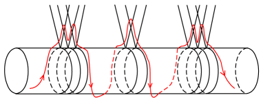
Figure 4.1. A global connecting orbit shadowing the generalized transition chain

5. Technical estimates on Gevrey functions

In this part, we provide some necessary results for Gevrey functions defined on the torus $\mathbb{T}^{n}=\mathbb{R}^{n}/\mathbb{Z}^{n}$, which will be useful for our choice of Gevrey space in section 6.3. We present this section in a self-contained way for the reader’s convenience.

The variational proof of the genericity of Arnold diffusion usually depends on the existence of functions with compact support, i.e. bump functions. This technique cannot apply to the problem of analytic genericity since no analytic function has compact support. However, the bump function does exist in the Gevrey-$\alpha$ category with $\alpha>1$. Here we give a modified Gevrey bump function which is based on the one constructed in [65].

Lemma 5.1 (Gevrey bump function).

Let $\alpha>1,\mathbf{L}>0$, $D=[a_{1},b_{1}]\times\cdots\times[a_{n},b_{n}]$$\varsubsetneq\mathbb{T}^{n}$ be a $n$-dimensional cube and $U$ be an open neighborhood of $D$. Then there exists $f\in\mathbf{G}^{\alpha,\mathbf{L}}(\mathbb{T}^{n})$ such that $0\leq f\leq 1$, $\textup{supp}f\subset U$, and

$$f(x)=1\Longleftrightarrow x\in D.$$

Proof.

We first claim that for $0<d<d^{\prime}<\frac{1}{2}$, there exists a function $g\in\mathbf{G}^{\alpha,\mathbf{L}}(\mathbb{T})$ such that $0\leq g\leq 1$ and

$$g(x)=1\Longleftrightarrow x\in[-d,d],\quad\textup{supp}g\subset[-d^{\prime},d^{\prime}].$$

Indeed, let $\alpha=1+\frac{1}{\sigma}$ ($\sigma>0$) and define a non-negative function $h\in C^{\infty}(\mathbb{R})$ as follows: $h(x)=0$ for $x\leq 0$, $h(x)=$$\exp(-\frac{\lambda}{x^{\sigma}})$ for $x>0$. Then $h\in\mathbf{G}^{\alpha,\mathbf{L}}(\mathbb{R})$ if the constant $\lambda>(2\mathbf{L}^{\alpha}/\sin a)^{\sigma}/\sigma$ with $a=\frac{\pi}{4}\min\{1,\frac{1}{\sigma}\}$ (cf. [64, Lemma A.3]). Next, we define $\psi(x)=\int_{-\infty}^{x}h\big{(}t+\frac{d^{\prime}-d}{2}\big{)}h\big{(}-t+\frac{d^{\prime}-d}{2}\big{)}~{}dt.$ It’s easy to compute that $\psi\geq 0$ is non-decreasing and

$$\psi(x)=\left\{\begin{array}[]{ll}0,&x\leq-\frac{d^{\prime}-d}{2}\\ K,&x\geq\frac{d^{\prime}-d}{2}\end{array}\right.$$

where

$$K=\int^{\frac{d^{\prime}-d}{2}}_{-\frac{d^{\prime}-d}{2}}h\big{(}t+\frac{d^{\prime}-d}{2}\big{)}h\big{(}-t+\frac{d^{\prime}-d}{2}\big{)}~{}dt>0.$$

Then we define the function

$$g(x)=\frac{1}{K^{2}}\psi\big{(}x+\frac{d^{\prime}+d}{2}\big{)}\psi\bigg{(}-x+\frac{d^{\prime}+d}{2}\big{)}.$$

Obviously, $0\leq g\leq 1$, $\textup{supp}g\subset[-d^{\prime},d^{\prime}]$, and $g(x)=1$ $\Longleftrightarrow$ $x\in[-d,d]$. It can be viewed as a function defined on $\mathbb{T}$. Hence by property (G1) in Section 1, $g\in\mathbf{G}^{\alpha,\mathbf{L}}(\mathbb{T})$, which proves our claim.

Next, without loss of generality we assume $D=[-d_{1},d_{1}]\times\cdots\times[-d_{n},d_{n}]$ with $0<d_{i}<\frac{1}{2}$. By assumption, we can find another cube $D^{\prime}=[-d^{\prime}_{1},d^{\prime}_{1}]\times\cdots\times[-d^{\prime}_{n},d^{\prime}_{n}]$ such that $D\subset D^{\prime}\subset U\subset\mathbb{T}^{n}$. By the claim above, for each $i\in\{1,\cdots,n\}$ there exists a function $f_{i}\in\mathbf{G}^{\alpha,\mathbf{L}}(\mathbb{T})$ such that $0\leq f_{i}\leq 1$, $\textup{supp}f_{i}\subset[-d_{i}^{\prime},d_{i}^{\prime}]$, $f_{i}(x)=1$ $\Longleftrightarrow$ $x\in[-d_{i},d_{i}]$. Thus we define

$$f(x_{1},\cdots,x_{n}):=\prod_{i=1}^{n}f_{i}(x_{i}),$$

which meets our requirements. ∎

Next, we prove that the inverse of a Gevrey map is still Gevrey smooth. For each high dimensional map $\varphi=(\varphi_{1},\cdots,\varphi_{n}):V\to\mathbb{R}^{n}$ where $\varphi_{i}\in\mathbf{G}^{\alpha,\mathbf{L}}(V)$, its norm could be defined as follows:

$$\|\varphi\|_{\alpha,\mathbf{L}}:=\sum\limits_{i=1}^{n}\|\varphi_{i}\|_{\alpha,\mathbf{L}}.$$

In what follows, $(0,1)^{n}$ denotes the unit domain $(0,1)\times\cdots\times(0,1)$ in $\mathbb{R}^{n}$. We also refer the reader to [51] for the inverse function theorem of a general ultra-differentiable mapping.

Theorem 5.2 (Inverse Function Theorem of Gevrey class).

Let $X,Y$ be two open sets in $(0,1)^{n}$ and let $f:X\to Y$ be a Gevrey-$(\alpha,\mathbf{L})$ map with $\alpha\geq 1$. If the Jacobian matrix $Jf$ is non-degenerate at $x_{0}\in X$, then there exist an open set $U$ containing $x_{0}$, an open set $V$ containing $f(x_{0})$, a constant $\mathbf{L}_{1}<\mathbf{L}$, and a unique inverse map $f^{-1}:V\to U$ such that $f^{-1}\in\mathbf{G}^{\alpha,\mathbf{L}_{1}}(V)$.

Proof.

For simplicity we suppose the Jacobian matrix $J_{x_{0}}f=I_{n}$ where $I_{n}=\textup{diag}(1,1,\cdots,1)$, otherwise we can replace $f$ by $f\circ(J_{x_{0}}f)^{-1}$. We also suppose $f(x_{0})=x_{0}$, otherwise we can replace $f$ by $f+x_{0}-f(x_{0})$. If we write $f=id+h$ in a neighborhood of $x_{0}$, then $h(x_{0})=0$, $J_{x_{0}}h=0$. For $0<\varepsilon\ll 1$ there exist $d>0$ and an open ball $B_{d}(x_{0})=$$\{x\in X:\|x-x_{0}\|<d\}$ such that

$$\quad\|h\|_{C^{1}(B_{d}(x_{0}))}\leq\varepsilon.$$ (5.1)

By classical Inverse Function Theorem, there exist two small open sets $U,V\subset B_{d/2}(x_{0})$ containing $x_{0}$ and a unique $C^{\infty}$ inverse map $f^{-1}:V\to U$ where $f^{-1}(x_{0})=x_{0}$. Let $\mathbf{L}_{1}=\varepsilon^{\frac{2}{3\alpha}}$, next we will prove $f^{-1}\in\mathbf{G}^{\alpha,\mathbf{L}_{1}}(V)$ by the contraction mapping principle.

We can write $f^{-1}=id+g$ , so $g\in C^{\infty}(V)$ and the equality

$$g(y)=-h(y+g(y)),~{}\forall y\in V$$

holds. Define the set $E=\{\varphi=(\varphi_{1},\cdots,\varphi_{n}):\varphi(x_{0})=0,~{}\varphi\in\mathbf{G}^{\alpha,\mathbf{L}_{1}}(V),~{}\|\varphi\|_{\alpha,\mathbf{L}_{1}}\leq\varepsilon^{\frac{3}{4}}\}$ with the norm $\|\cdot\|_{\alpha,\mathbf{L}_{1}}$, it’s a non-empty, closed and convex set in the space $\mathbf{G}^{\alpha,\mathbf{L}_{1}}(V)$. Define the operator

$$(T\varphi)(y):=-h(y+\varphi(y)),\forall y\in V.$$

$\bullet$ We first claim that the mapping $T\varphi\in E,$ $\forall\varphi\in E.$ In fact, for each $\varphi\in E$, $(T\varphi)(x_{0})=0$. For $y\in V\subset B_{d/2}(x_{0})$, we have $\|y+\varphi(y)-x_{0}\|\leq\|y-x_{0}\|+\|\varphi(y)-\varphi(x_{0})\|\leq\frac{d}{2}+\|J\varphi\|\|y-x_{0}\|<d$, and hence $(id+\varphi)(V)$$\subset B_{d}(x_{0})$. Moreover, let $\mathbf{L}_{2}:=\mathbf{L}\varepsilon^{\frac{1}{2\alpha}}$ and $\varepsilon$ be suitably small. For each $i\in\{1,\cdots,n\}$,

$$\begin{split}\|x_{i}+\varphi_{i}\|_{\alpha,\mathbf{L}_{1}}-\|x_{i}+\varphi_{i}\|_{C^{0}}=&\sum\limits_{j=1}^{n}\mathbf{L}_{1}^{\alpha}\|\delta_{ij}+\partial_{x_{j}}\varphi_{i}\|_{C^{0}}+\sum\limits_{k\in\mathbb{N}^{n},|k|\geq 2}\frac{\mathbf{L}_{1}^{|k|\alpha}}{(k!)^{\alpha}}\|\partial^{k}\varphi_{i}\|_{C^{0}}\\ \leq&n\mathbf{L}_{1}^{\alpha}(1+\frac{\varepsilon^{\frac{3}{4}}}{\mathbf{L}_{1}^{\alpha}})+\|\varphi_{i}\|_{\alpha,\mathbf{L}_{1}}\leq 2n\varepsilon^{\frac{2}{3}}+\varepsilon^{\frac{3}{4}}\leq\frac{\mathbf{L}_{2}^{\alpha}}{n^{\alpha-1}},\end{split}$$

where $\delta_{ij}=1$ for $i=j$ and $\delta_{ij}=0$ for $i\neq j$. Hence by property (G3) in Section 1, $\|T\varphi\|_{\alpha,\mathbf{L}_{1}}=\|h\circ(id+\varphi)\|_{\alpha,\mathbf{L}_{1}}\leq\|h\|_{\alpha,\mathbf{L}_{2},B_{d}(x_{0})}$ since $(id+\varphi)(V)$$\subset B_{d}(x_{0})$. Now it only remains to verify that

$$\|h\|_{\alpha,\mathbf{L}_{2},B_{d}(x_{0})}\leq\varepsilon^{\frac{3}{4}}.$$

Recall that for $|k|\geq 2$ and $x\in B_{d}(x_{0})$, $\partial^{k}f_{i}(x)=\partial^{k}h_{i}(x)$. By using (5.1), we have

$$\begin{split}\|h_{i}\|_{\alpha,\mathbf{L}_{2},B_{d}(x_{0})}&=\|h_{i}\|_{C^{0}(B_{d}(x_{0}))}+\sum\limits_{k\in\mathbb{N}^{n},|k|=1}\mathbf{L}_{2}^{\alpha}\|\partial^{k}h_{i}\|_{C^{0}(B_{d}(x_{0}))}+\sum\limits_{k\in\mathbb{N}^{n},|k|\geq 2}\frac{\mathbf{L}_{2}^{|k|\alpha}}{k!^{\alpha}}\|\partial^{k}f_{i}\|_{C^{0}(B_{d}(x_{0}))}\\ &\leq(1+n\mathbf{L}_{2}^{\alpha})\varepsilon+\sum\limits_{k\in\mathbb{N}^{n},|k|\geq 2}\frac{\mathbf{L}^{|k|\alpha}\varepsilon^{\frac{|k|}{2}}}{k!^{\alpha}}\|\partial^{k}f_{i}\|_{C^{0}(B_{d}(x_{0}))}\\ &\leq(1+n\mathbf{L}^{\alpha}\varepsilon^{\frac{1}{2}})\varepsilon+\varepsilon\|f\|_{\alpha,\mathbf{L}}\leq\frac{\varepsilon^{\frac{3}{4}}}{n},\end{split}$$ (5.2)

which proves the claim.

$\bullet$ On the other hand, for $\varphi,\tilde{\varphi}\in E$ and $i\in\{1,\cdots,n\}$, by the Newton-Leibniz formula we have

$$\begin{split}h_{i}(x+\varphi(x))-h_{i}(x+\tilde{\varphi}(x))=&\bigg{(}\int_{0}^{1}Jh_{i}\big{(}x+s\varphi(x)+(1-s)\tilde{\varphi}(x)\big{)}ds\bigg{)}\bigg{(}\varphi(x)-\tilde{\varphi}(x)\bigg{)}\\ =&F(x)\big{(}\varphi(x)-\tilde{\varphi}(x)\big{)}\end{split}$$

where $Jh_{i}$ is the Jacobian matrix. It follows from property (G2) in Section 1 and (5.2) that

$$\|Jh_{i}\|_{\alpha,\frac{\mathbf{L}_{2}}{2},B_{d}(x_{0})}\leq\frac{\|h_{i}\|_{\alpha,\mathbf{L}_{2},B_{d}(x_{0})}}{(\mathbf{L}_{2}-\mathbf{L}_{2}/2)^{\alpha}}\sim O(\varepsilon^{\frac{1}{4}})<\frac{1}{2n}$$

provided $\varepsilon$ is suitably small. By property (G3), $\|F\|_{{\alpha,\mathbf{L}_{1},V}}\leq\|Jh_{i}\|_{\alpha,\frac{\mathbf{L}_{2}}{2},B_{d}(x_{0})}\leq\frac{1}{2n}$.

Finally, we deduce from (G1) that

$$\|h_{i}\circ(id+\varphi)-h_{i}\circ(id+\tilde{\varphi})\|_{\alpha,\mathbf{L}_{1}}\leq\|F\|_{\alpha,\mathbf{L}_{1}}\|\varphi-\tilde{\varphi}\|_{\alpha,\mathbf{L}_{1}}\leq\frac{1}{2n}\|\varphi-\tilde{\varphi}\|_{\alpha,\mathbf{L}_{1}}.$$

Hence $\|h\circ(id+\varphi)-h\circ(id+\tilde{\varphi})\|_{\alpha,\mathbf{L}_{1}}\leq\frac{1}{2}\|\varphi-\tilde{\varphi}\|_{\alpha,\mathbf{L}_{1}}$, namely

$$\|T\varphi-T\tilde{\varphi}\|_{\alpha,\mathbf{L}_{1}}\leq\frac{1}{2}\|\varphi-\tilde{\varphi}\|_{\alpha,\mathbf{L}_{1}}.$$

In conclusion, $T:E\to E$ is a contraction mapping. By the contraction mapping principle, $T$ has a unique fixed point, and hence the fixed point must be $g$. Therefore, $f^{-1}=id+g\in\mathbf{G}^{\alpha,\mathbf{L}_{1}}(V)$. ∎

Sometimes we need to approximate a continuous function by Gevrey smooth ones. Convolution provides us with a systematic technique. More specifically, for any $\alpha>1,\mathbf{L}>0$, by Lemma 5.1 there exists a non-negative function $\eta\in\mathbf{G}^{\alpha,\mathbf{L}}(\mathbb{R}^{n})$ such that $\textup{supp}\eta$ $\subset[\frac{1}{4},\frac{3}{4}]^{n}$ and $\int_{\mathbb{R}^{n}}\eta(x)dx=1$. Next we set $\eta_{\varepsilon}(x)=\frac{1}{\varepsilon^{n}}\eta(\frac{x}{\varepsilon})$ $(0<\varepsilon<1,x\in\mathbb{R}^{n})$ which is called the mollifier. Then we define the convolution of $\eta_{\varepsilon}$ and $f\in C^{0}(\mathbb{T}^{n})$ by

$$\eta_{\varepsilon}*f(x)=\int_{\mathbb{T}^{n}}\eta_{\varepsilon}(x-y)f(y)dy,~{}\forall~{}x\in\mathbb{T}^{n}.$$ (5.3)

Theorem 5.3 (Gevrey approximation).

1. Let $\alpha>1$, and $U\subset\mathbb{T}^{n}$, $V\subsetneq(0,1)^{n}$ be two open sets. If $f:U\to V$ is a continuous map, then there exists a sequence of maps $f^{\varepsilon}:U\to(0,1)^{n}$ such that $f^{\varepsilon}\in\mathbf{G}^{\alpha,\mathbf{L}_{\varepsilon}}(U)$. Furthermore, $\mathbf{L}_{\varepsilon}\to 0$ and $\|f^{\varepsilon}-f\|_{C^{0}}\to 0$ as $\varepsilon$ tends to 0.

2. Let $\alpha>1$, $U,V$ be connected open sets satisfying $\bar{U},\bar{V}\varsubsetneq\mathbb{T}^{n}$ and $f:U\to V$ be a continuous map. Then there exists a sequence of maps $f^{\varepsilon}:U\to\mathbb{T}^{n}$ such that $f^{\varepsilon}\in\mathbf{G}^{\alpha,\mathbf{L}_{\varepsilon}}(U)$, $\mathbf{L}_{\varepsilon}\to 0$ and $\|f^{\varepsilon}-f\|_{C^{0}}\to 0$ as $\varepsilon$ tends to 0. Specifically, if $f$ is a diffeomorphism and the determinant $\det(Jf)$ ($Jf$ is the Jacobian matrix) has a uniform positive distance away from zero, then the Gevrey map $f^{\varepsilon}:U\to V^{\varepsilon}$ with $V^{\varepsilon}=f^{\varepsilon}(U)$ will also be a diffeomorphism provided that $\varepsilon$ is small enough.

Proof.

(1): Let $f=(f_{1},\cdots,f_{n})$ and $f_{i}$ ($1\leq i\leq n$) be continuous, we only need to prove that each $f_{i}$ can be approximated by a Gevrey smooth function. Indeed, let $f_{i}^{\varepsilon}=\eta_{\varepsilon}*f_{i}$ ($0<\varepsilon<1$), where $\eta\in\mathbf{G}^{\alpha,\mathbf{L}}$. It’s easy to check that $f_{i}^{\varepsilon}:U\to(0,1)$ since $\int_{\mathbb{R}^{n}}\eta_{\varepsilon}(x)dx=1$ and $\textup{supp}\eta_{\varepsilon}$$\subset[\frac{\varepsilon}{4},\frac{3\varepsilon}{4}]^{n}$. By the classical properties of convolutions, one obtains $f^{\varepsilon}_{i}\in C^{\infty}$ and

$$\|f_{i}^{\varepsilon}-f_{i}\|_{C^{0}}\to 0,\textup{~{}as~{}}\varepsilon\to 0.$$

$$\partial^{k}f^{\varepsilon}_{i}=\partial^{k}\eta_{\varepsilon}*f_{i}=\int_{\mathbb{T}^{n}}\partial^{k}\eta_{\varepsilon}(x-y)f_{i}(y)dy,~{}\forall~{}k=(k_{1},\cdots,k_{n})\in\mathbb{Z}^{n},k_{i}\geq 0.$$

It only remains to prove $f_{i}^{\varepsilon}$ is Gevrey smooth. In fact, if one sets $\mathbf{L}_{\varepsilon}=\mathbf{L}\varepsilon^{\frac{1}{\alpha}}$, then

$$\begin{split}\|f^{\varepsilon}_{i}\|_{\alpha,\mathbf{L}_{\varepsilon}}&\leq\sum\limits_{k}\frac{\mathbf{L}_{\varepsilon}^{|k|\alpha}}{k!^{\alpha}}\|\partial^{k}\eta_{\varepsilon}\|_{C^{0}}\|f_{i}\|_{C^{0}}\\ &\leq\frac{\|f_{i}\|_{C^{0}}}{\varepsilon^{n}}\sum\limits_{k}\frac{\mathbf{L}_{\varepsilon}^{|k|\alpha}\varepsilon^{-|k|}}{k!^{\alpha}}\|\partial^{k}\eta\|_{C^{0}}\\ &=\frac{\|f_{i}\|_{C^{0}}}{\varepsilon^{n}}\sum\limits_{k}\frac{\mathbf{L}^{|k|\alpha}}{k!^{\alpha}}\|\partial^{k}\eta\|_{C^{0}}=\frac{\|f_{i}\|_{C^{0}}}{\varepsilon^{n}}\|\eta\|_{\alpha,\mathbf{L}}.\end{split}$$

Obviously, $\mathbf{L}_{\varepsilon}\to 0$ as $\varepsilon\to 0$. This completes the proof of (1).

(2): The first part is not hard to prove by the technique in (1). Furthermore, if $f$ is a diffeomorphism from $U$ to $V$, then by using $\partial^{k}f^{\varepsilon}=\eta_{\varepsilon}*\partial^{k}f$ with $|k|=1$, one gets

$$\|f^{\varepsilon}-f\|_{C^{1}}\to 0,\quad\varepsilon\to 0.$$ (5.4)

Since $\det(Jf)$ has a uniform positive distance away from zero, it concludes from (5.4) and Theorem 5.2 that $f^{\varepsilon}:U\to f^{\varepsilon}(U)$ would also be a diffeomorphism for $\varepsilon$ small enough. ∎

6. Proof of the main results

This section is the main part of the present paper, which aims to prove Theorem 1.2 and Theorem 1.3. We will explain how to apply the tools exposed in the previous sections to a priori unstable and Gevrey smooth systems. Before that, we need to do some preparations.

6.1. Genericity of uniquely minimal measure in Gevrey or analytic topology

Let $M=\mathbb{T}^{n}$. We fix an $h\in H_{1}(M,\mathbb{R})$, it is well known that in the $C^{r}$ ($2\leq r\leq\infty$) topology, a generic Lagrangian has only one minimal measure $\mu$ with the rotation vector $\rho(\mu)=h$ (see [61]). Next, we will show that such a property still holds in the Gevrey topology. For this purpose, we shall consider it in a Gevrey space $\mathbf{G}^{\alpha,\mathbf{L}}(M\times\mathbb{T})$ with $\alpha\geq 1,\mathbf{L}>0$. A property is called generic in the sense of Mañé if, for each Lagrangian $L:TM\times\mathbb{T}\to\mathbb{R}$, there exists a residual subset $\mathcal{O}\subset\mathbf{G}^{\alpha,\mathbf{L}}(M\times\mathbb{T})$ such that the property holds for each Lagrangian $L+\phi$ with $\phi\in\mathcal{O}$.

Theorem 6.1.

Let $h\in H_{1}(M,\mathbb{R})$, $\alpha\geq 1,\mathbf{L}>0$ and $L:TM\times\mathbb{T}\to\mathbb{R}$ be a Tonelli Lagrangian, then there exists a residual subset $\mathcal{O}(h)\subset\mathbf{G}^{\alpha,\mathbf{L}}(M\times\mathbb{T})$ such that, for each $\phi\in\mathcal{O}(h)$, the Lagrangian $L+\phi$ has only one minimal measure with the rotation vector $h$.

Remark.

We shall note that the residual set $\mathcal{O}(h)$ depends on the homology class $h$.

Proof.

Recall Mañé’s equivalent definition of minimal measure in Section 2, we are going to prove this theorem in the following setting based on Mañé’s approach.

1. Set $E:=\mathbf{G}^{\alpha,\mathbf{L}}(M\times\mathbb{T}).$ Obviously, it is a Banach space.

2. Denote by $F\subset\mathrm{C}^{*}$ the vector space spanned by the set of probability measures $\mu\in\mathcal{H}$ with $\int_{TM\times\mathbb{T}}L\,d\mu<\infty$, the definitions of the sets $\mathcal{H}$ and $\mathrm{C}^{*}$ are in Section 2. Recall that for $\mu_{k},\mu\in F$,

   $$\lim\limits_{k\to+\infty}\,\mu_{k}=\mu\Longleftrightarrow\lim\limits_{k\to+\infty}\int_{TM\times\mathbb{T}}f\,d\mu_{k}=\int_{TM\times\mathbb{T}}fd\mu,\quad\forall f\in\mathrm{C}.$$

3. Let $\mathcal{L}:F\to\mathbb{R}$ be a linear map satisfying $\mathcal{L}(\mu)=\int L\,d\mu$, for every $\mu\in F$.

4. Let $\varphi:E\to F^{*}$ be a linear map such that for each $\phi\in E$, $\varphi(\phi)\in F^{*}$ is defined as follows

   $$\langle\varphi(\phi),\mu\rangle:=\int\phi\,d\mu,~{}\mu\in F.$$

5. $K:=\{\mu\in F~{}|~{}\rho(\mu)=h\}$. It’s easy to check that $K$ is a separable metrizable convex subset.

For $\phi\in E$, we denote

$$\arg\min(\phi):=\{~{}\mu\in K~{}|~{}\mathcal{L}(\mu)+\langle\varphi(\phi),\mu\rangle=\min\limits_{\nu\in K}(\mathcal{L}(\nu)+\langle\varphi(\phi),\nu\rangle)~{}\}.$$

It’s easy to verify that our setting above satisfies all conditions of that in [61, Proposition 3.1], so there exists a residual subset $\mathcal{O}(h)\subset E$ such that each $\phi\in\mathcal{O}(h)$ has the following property:

$$\#\arg\min(\phi)=1.$$

Since $\arg\min(\phi)$ $=$ $\mathfrak{H}_{h}(L+\phi)$, see (2.7), it follows from Proposition 2.2 that the Lagrangian $L+\phi$ admits only one minimal measure with the rotation vector $h$. ∎

Remark.

For $\alpha=1$, $\mathbf{G}^{1,\mathbf{L}}$ is the space of real analytic functions. This therefore means that the uniqueness of minimal measure is also a generic property in the analytic topology.

Corollary 6.2.

Let $\mathbf{L}>0$, $\alpha\geq 1$ and $L:T\mathbb{T}^{n}\times\mathbb{T}$ be a Tonelli Lagrangian. Then there exists a residual set $\mathcal{O}_{1}\subset\mathbf{G}^{\alpha,\mathbf{L}}(\mathbb{T}^{n}\times\mathbb{T})$ such that for any $V\in\mathcal{O}_{1}$, the Lagrangian $L+V$ has the following property: for each rational $h=(h_{1},\cdots,h_{n})\in H_{1}(\mathbb{T}^{n},\mathbb{R})$ with $h_{i}\in\mathbb{Q}$, $L+V$ has one and only one minimal measure with the rotation vector $h$.

Proof.

For each $h\in H_{1}(\mathbb{T}^{n},\mathbb{R})$, thanks to Theorem 6.1, we obtain a residual subset $\mathcal{O}(h)\subset\mathbf{G}^{\alpha,\mathbf{L}}(\mathbb{T}^{n}\times\mathbb{T})$ such that for each $\phi\in\mathcal{O}(h)$, the Lagrangian $L+\phi$ has only one minimal measure with the rotation vector $h$. Then we set

$$\mathcal{O}_{1}=\bigcap_{h\in\mathbb{Q}^{n}}\mathcal{O}(h),$$

which is the intersection of countably many residual sets. Of course, by the definition of residual set, $\mathcal{O}_{1}$ is non-empty and still residual (also dense) in the Banach space $\mathbf{G}^{\alpha,\mathbf{L}}(\mathbb{T}^{n}\times\mathbb{T})$. The corollary is now evident from what we have proved. ∎

6.2. Hölder regularity of elementary weak KAM solutions

In this part, we will choose a family of elementary weak KAM solutions which can be parameterized so that they are Hölder continuous in the $C^{0}$ topology. Such a property is crucial for our proof of Theorem 6.7.

To this end, we need to do study the normally hyperbolic cylinders (refer to Appendix A). Let us go back to our two and a half degrees of freedom Hamiltonian model (1.2). Let

$$\Sigma(0):=\{(q_{1},0,p_{1},0):q_{1}\in\mathbb{T},|p_{1}|\leq R\}\subset\mathbb{T}^{2}\times\mathbb{R}^{2}.$$

It is a cylinder restricted on the time-$0$ section, where $R$ is the constant fixed in Section 1. By condition (H2), $\Sigma(0)$ is a normally hyperbolic invariant cylinder (NHIC) for the time-1 map of the Hamiltonian flow $\Phi_{H_{0}}^{t}$. Since the Hamiltonian $H_{0}$ is integrable when restricted in the cylinder $\Sigma(0)$, the rate $\mu$ in (A.1) is 1 and $\log\mu=0$, so it follows from Theorem A.3 that there exists

$$\varepsilon_{1}=\varepsilon_{1}(H_{0},R)>0$$ (6.1)

such that if $\|H_{1}\|_{C^{3}(\mathscr{D}_{R})}\leq\varepsilon_{1}$, the time-1 map $\Phi_{H}^{1}$ of the Hamiltonian $H$ still admits a $C^{r-1}$ normally hyperbolic invariant cylinder $\Sigma_{H}(0)$, which is a small deformation of $\Sigma(0)$ and can be considered as the image of the following diffeomorphism (see figure 6.1)

$$\begin{split}\psi:\Sigma(0)&\to\Sigma_{H}(0)\subset\mathbb{T}^{2}\times\mathbb{R}^{2},\\ (q_{1},0,p_{1},0)&\mapsto(q_{1},\mathbf{q}_{2}(q_{1},p_{1}),p_{1},\mathbf{p}_{2}(q_{1},p_{1})).\end{split}$$ (6.2)

Here, $\mathbf{q}_{2}$ and $\mathbf{p}_{2}$ are two $C^{r-1}$ functions taking values close to zero. Then $\psi$ induces a 2-form $\psi^{*}\Omega$ on the standard cylinder $\Sigma(0)$ where $\Omega=\sum_{i=1}^{2}dq_{i}\wedge dp_{i}$,

$$\psi^{*}\Omega=\bigg{(}1+\frac{\partial(\mathbf{q}_{2},\mathbf{p}_{2})}{\partial(q_{1},p_{1})}\bigg{)}dq_{1}\wedge dp_{1}.$$

Since the second de Rham cohomology group $H^{2}(\Sigma(0),\mathbb{R})=\{0\}$, by using Moser’s trick on the isotopy of symplectic forms, one can find a diffeomorphism $\psi_{1}:\Sigma(0)\to\Sigma(0)$ such that

$$\psi_{1}^{*}\psi^{*}\Omega=dq_{1}\wedge dp_{1}.$$

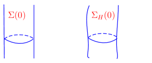
Figure 6.1. $\Sigma_{H}(0)$ is a small deformation of $\Sigma(0)$

Recall that $\Sigma_{H}(0)$ is invariant under $\Phi_{H}^{1}$ and $(\Phi_{H}^{1})^{*}\Omega=\Omega$, one obtains

$$\big{(}(\psi\circ\psi_{1})^{-1}\circ\Phi_{H}^{1}\circ(\psi\circ\psi_{1})\big{)}^{*}dq_{1}\wedge dp_{1}=dq_{1}\wedge dp_{1}.$$

Combining with the fact that $(\psi\circ\psi_{1})^{-1}\circ\Phi_{H}^{1}\circ(\psi\circ\psi_{1})$ is a small perturbation of $\Phi_{H_{0}}^{1}$, the map $(\psi\circ\psi_{1})^{-1}\circ\Phi_{H}^{1}\circ(\psi\circ\psi_{1})$ is an exact twist map, and hence one can apply the classical Aubry-Mather theory to characterize the minimal orbits on $\Sigma(0)$: given a $\rho\in\mathbb{R}$, there exists an Aubry-Mather set with rotation number $\rho$ satisfying

1. if $\rho\in\mathbb{Q}$, the set consists of periodic orbits.

2. if $\rho\in\mathbb{R}\setminus\mathbb{Q}$, the set is either an invariant circle or a Denjoy set.

For simplicity, we denote by

$$\Sigma_{H}(s)=\Phi^{s}_{H}(\Sigma_{H}(0),0),\quad\Sigma(s)=\Phi^{s}_{H_{0}}(\Sigma(0),0)$$

the 2-dimensional manifolds, and denote by

$$\widetilde{\Sigma}_{H}=\bigcup_{s\in\mathbb{T}}\Sigma_{H}(s),\quad\widetilde{\Sigma}=\bigcup_{s\in\mathbb{T}}\Sigma(s)$$ (6.3)

the 3-dimensional manifolds in $T^{*}\mathbb{T}^{2}\times\mathbb{T}$. By using the Legendre transformation $\mathscr{L}$ (see (1.4)), the set $\mathscr{L}\widetilde{\Sigma}_{H}$ is $\phi_{L}^{t}$-invariant in $T\mathbb{T}^{2}\times\mathbb{T}$. Given a cohomology class $c=(c_{1},0)\in H^{1}(\mathbb{T}^{2},\mathbb{R})$ with $|c_{1}|\leq R-1$, the following lemma shows that the Aubry set $\widetilde{\mathcal{A}}(c)$ lies inside the cylinder $\mathscr{L}\widetilde{\Sigma}_{H}$.

Lemma 6.3 (Location of the minimal sets).

Let $H$ be the Hamiltonian (1.2) and $L$ be the associated Lagrangian (1.3). There exists $\varepsilon_{1}=\varepsilon_{1}(H_{0},R)>0$ such that if $\|H_{1}\|_{C^{3}(\mathscr{D}_{R})}\leq\varepsilon_{1}$ , then for each $c=(c_{1},0)$ with $|c_{1}|\leq R-1$, the globally minimal set $\widetilde{\mathcal{G}}_{L}(c)\subset\mathscr{L}\widetilde{\Sigma}_{H}$.

Proof.

We first consider the autonomous Lagrangian $l_{2}(q_{2},v_{2})$. It follows from (1.5) that $(0,0)$ is the unique minimal point of $l_{2}$, so the globally minimal set of the Lagrangian $l_{2}$ is

$$\widetilde{\mathcal{G}}_{l_{2}}=(0,0)\times\mathbb{T}\subset T\mathbb{T}\times\mathbb{T}.$$

Then for all $c=(c_{1},0)$ with $|c_{1}|\leq R$, the globally minimal set of $L_{0}=l_{1}(v_{1})+l_{2}(q_{2},v_{2})$ is

$$\widetilde{\mathcal{G}}_{L_{0}}(c)=\{(q_{1},0,Dh_{1}(c_{1}),0,t)~{}:~{}q_{1}\in\mathbb{T},t\in\mathbb{T}\}\textup{~{}and~{}}\widetilde{\mathcal{G}}_{L_{0}}(c)\subset\mathscr{L}\widetilde{\Sigma}.$$

Here, the function $h_{1}$ is given in (1.2).

Next, we take a small neighborhood $U$ of $\mathscr{L}\widetilde{\Sigma}$ in the space $T\mathbb{T}^{2}\times\mathbb{T}$ and let $\varepsilon_{1}=\varepsilon_{1}(H_{0},R)$ be the constant defined in (6.1). Since $\|H_{1}\|_{C^{3}(\mathscr{D}_{R})}\leq\varepsilon_{1}$, by letting $\varepsilon_{1}$ suitably small, it follows that $\|L_{1}\|_{C^{2}(\mathscr{D}_{R})}$ is also sufficiently small. Thus, by the upper semi-continuity in Proposition 2.1, $\widetilde{\mathcal{G}}_{L}(c)\subset U$ for all $c\in[-R+1,R-1]\times\{0\}$ where $L=L_{0}+L_{1}$. Equivalently,

$$\mathscr{L}^{-1}\widetilde{\mathcal{G}}_{L}(c)\subset\mathscr{L}^{-1}U.$$

On the other hand, due to normal hyperbolicity and Theorem A.3,

$$\widetilde{\Sigma}_{H}\subset\mathscr{L}^{-1}U,$$

provided that $\varepsilon_{1}$ is small enough. Moreover, $\widetilde{\Sigma}_{H}$ is the unique $\phi^{t}_{L}$-invariant set in the neighborhood $\mathscr{L}^{-1}U$. This therefore implies $\mathscr{L}^{-1}\widetilde{\mathcal{G}}_{L}(c)\subset\widetilde{\Sigma}_{H}$ since $\mathscr{L}^{-1}\widetilde{\mathcal{G}}_{L}(c)$ is $\phi^{t}_{L}$-invariant. ∎

In the remainder of this section, we will use the following notation for simplicity.

Notation:

1. In what follows, we use $M$ to denote the manifold $\mathbb{T}^{2}=\mathbb{R}^{2}/\mathbb{Z}^{2}$. Also, we denote by

   $$\check{M}=\mathbb{T}\times 2\mathbb{T}=\mathbb{R}/\mathbb{Z}\times\mathbb{R}/2\mathbb{Z},\quad\check{\pi}:\check{M}\to M$$

   the double covering of $M$. We use such a double covering to distinguish between $0$ and $1$ in the $q_{2}$-coordinate, and identify 0 with 2 in the $q_{2}$-coordinate.

   The Hamiltonian $H:T^{*}M\times\mathbb{T}\to\mathbb{R}$ and the Lagrangian $L:TM\times\mathbb{T}\to\mathbb{R}$ could extend naturally to $T^{*}\check{M}$ and $T\check{M}$ respectively. By abuse of notation, we continue to write $H:T^{*}\check{M}\times\mathbb{T}\to\mathbb{R}$ and $L:T\check{M}\times\mathbb{T}\to\mathbb{R}$ for the new Hamiltonian and Lagrangian respectively. In this setting, the lift of the NHIC $\Sigma_{H}(0)$ will have two copies

   $$\check{\pi}^{-1}\Sigma_{H}(0)=\Sigma_{H,l}(0)\cup\Sigma_{H,u}(0),$$

   where the subscripts $l,u$ are introduced to indicate “lower” and “upper” respectively. Then $\check{\pi}^{-1}\widetilde{\Sigma}_{H}=\widetilde{\Sigma}_{H,l}\cup\widetilde{\Sigma}_{H,u}$.

2. For simplicity, we always use $\pi_{q}$ to denote the natural projection from $T\check{M}$ (resp. $TM$) to $\check{M}$ (resp. $M$) or from $T^{*}\check{M}$ (resp. $T^{*}M$) to $\check{M}$ (resp. $M$).

3. Let $\kappa>0$ be small, we denote by $\mathrm{U}_{\kappa}=\mathrm{U}_{\kappa,l}\cup\mathrm{U}_{\kappa,u}$ the disconnected subset in $\check{M}$ where

   $$\mathrm{U}_{\kappa,l}=\mathbb{T}\times[\kappa,1-\kappa],\quad\mathrm{U}_{\kappa,u}=\mathbb{T}\times[1+\kappa,2-\kappa].$$

   Let $\mathrm{N}_{\kappa}=\check{M}\setminus\mathrm{U}_{\kappa}=\mathrm{N}_{\kappa,l}\cup\mathrm{N}_{\kappa,u}$ where

   $$\mathrm{N}_{\kappa,l}=\mathbb{T}\times(-\kappa,\kappa),\quad\mathrm{N}_{\kappa,u}=\mathbb{T}\times(1-\kappa,1+\kappa).$$

   The subscripts $l,u$ are also introduced to indicate the “lower” and the “upper” respectively (See figure 6.4). The number $\kappa$ should be chosen such that

   $$\pi_{q}\circ\Sigma_{H,l}(0)\subset\mathrm{N}_{\kappa/2,l},\qquad\pi_{q}\circ\Sigma_{H,u}(0)\subset\mathrm{N}_{\kappa/2,u}.$$

   Namely, the perturbed cylinder is contained in a $\kappa/2$-neighborhood of the unperturbed one. Also, we let

   $$\widetilde{\Sigma}_{H,l}\subset\mathrm{N}_{\kappa/2,l}\times\mathbb{R}^{2}\times\mathbb{T},\quad\widetilde{\Sigma}_{H,u}\subset\mathrm{N}_{\kappa/2,u}\times\mathbb{R}^{2}\times\mathbb{T}.$$ (6.4)

4. For $c=(c_{1},0)$$\in H^{1}(M,\mathbb{R})$, if the Aubry set $\widetilde{\mathcal{A}}_{L}(c,M)|_{t=0}$ is an invariant circle, we denote by

   $$\Upsilon_{c}=\mathscr{L}^{-1}\widetilde{\mathcal{A}}_{L}(c,M)|_{t=0}\subset T^{*}M\times\{t=0\}$$

   the invariant circle in the cotangent space. This leads us to introduce an index set

   $$\mathbb{S}:=\{(c_{1},0)~{}:~{}|c_{1}|\leq R-1,~{}\Upsilon_{c}\textup{~{}is an invariant circle lying in~{}}\Sigma_{H}(0)\}.$$ (6.5)

5. Let $\mathbf{r_{0}}>0$ be small satisfying $\mathbf{r_{0}}>\kappa$. Since $\Sigma_{H}(0)$ is a NHIM for the time-1 map $\Phi_{H}^{1}$, we have the associated local stable and unstable manifolds, denoted by $W_{\Sigma_{H}(0)}^{s,loc}$ and $W_{\Sigma_{H}(0)}^{u,loc}$ respectively, in the $\mathbf{r_{0}}$-tubular neighborhood of $\Sigma_{H}(0)$. In addition, $W^{s,loc}_{\Sigma_{H}(0)}=\bigcup_{q\in\Sigma_{H}(0)}W^{s,loc}_{q}$ and $W^{u,loc}_{\Sigma_{H}(0)}=\bigcup_{q\in\Sigma_{H}(0)}W^{u,loc}_{q}$.

Now, let us focus on $c=(c_{1},0)\in\mathbb{S}$. For the $\Phi^{1}_{H}$-invariant circle $\Upsilon_{c}$, it has local stable manifold $W^{s,loc}_{\Upsilon_{c}}=\bigcup_{q\in\Upsilon_{c}}W^{s,loc}_{q}$ and local unstable manifold $W^{u,loc}_{\Upsilon_{c}}=\bigcup_{q\in\Upsilon_{c}}W^{u,loc}_{q}$. Theorem A.2 tells us that the leaf $W^{s,loc}_{q}$ (resp. $W^{u,loc}_{q}$) has smooth dependence on the base point $q\in\Sigma_{H}(0)$. Consequently, $W^{s,loc}_{\Upsilon_{c}}$ (resp. $W^{u,loc}_{\Upsilon_{c}}$) is a Lipschitz manifold since $\Upsilon_{c}$ is only Lipschitz in general. Besides, the local stable (unstable) manifold can be viewed as a Lipschitz graph over $\check{\pi}\circ\mathrm{N}_{\mathbf{r_{0}}}$, namely

$$\begin{split}W^{s,loc}_{\Upsilon_{c}}&=\{\big{(}q_{1},q_{2},\mathbf{p}_{1}^{s}(q_{1},q_{2}),\mathbf{p}_{2}^{s}(q_{1},q_{2})\big{)}\in T^{*}M\times\{t=0\}:(q_{1},q_{2})\in\check{\pi}\circ\mathrm{N}_{\mathbf{r_{0}}}\}\\ W^{u,loc}_{\Upsilon_{c}}&=\{\big{(}q_{1},q_{2},\mathbf{p}_{1}^{u}(q_{1},q_{2}),\mathbf{p}_{2}^{u}(q_{1},q_{2})\big{)}\in T^{*}M\times\{t=0\}:(q_{1},q_{2})\in\check{\pi}\circ\mathrm{N}_{\mathbf{r_{0}}}\}\end{split}$$

Here, $\mathbf{p}_{1}^{s,u},\mathbf{p}_{2}^{s,u}$ are Lipschitz functions on $\check{\pi}\circ\mathrm{N}_{\mathbf{r_{0}}}\subset M$, and the domain $\mathrm{N}_{\mathbf{r_{0}}}=\mathrm{N}_{\mathbf{r_{0}},l}\cup\mathrm{N}_{\mathbf{r_{0}},u}$ with

$$\mathrm{N}_{\mathbf{r_{0}},l}=\mathbb{T}\times(-\mathbf{r_{0}},\mathbf{r_{0}}),\quad\mathrm{N}_{\mathbf{r_{0}},u}=\mathbb{T}\times(1-\mathbf{r_{0}},1+\mathbf{r_{0}}).$$

Next, in the covering space $\check{M}$, the Aubry set $\widetilde{\mathcal{A}}_{L}(c,\check{M})$ is the union of two disjoint copies of $\widetilde{\mathcal{A}}_{L}(c,M)$ satisfying $\check{\pi}\widetilde{\mathcal{A}}_{L}(c,\check{M})=\widetilde{\mathcal{A}}_{L}(c,M)$. More precisely, $\mathscr{L}^{-1}\widetilde{\mathcal{A}}_{L}(c,\check{M})\big{|}_{t=0}=\Upsilon_{c,l}\cup\Upsilon_{c,u}$, where $\Upsilon_{c,\imath}$ lies in $\Sigma_{H,\imath}(0)$ and its stable and unstable manifolds are

$$\begin{split}W^{s,loc}_{\Upsilon_{c,\imath}}&=\{\big{(}q_{1},q_{2},\mathbf{p}_{1}^{s}(q_{1},q_{2}),\mathbf{p}_{2}^{s}(q_{1},q_{2})\big{)}\in T^{*}\check{M}\times\{t=0\}:(q_{1},q_{2})\in\mathrm{N}_{\mathbf{r_{0}},\imath}\}\\ W^{u,loc}_{\Upsilon_{c,\imath}}&=\{\big{(}q_{1},q_{2},\mathbf{p}_{1}^{u}(q_{1},q_{2}),\mathbf{p}_{2}^{u}(q_{1},q_{2})\big{)}\in T^{*}\check{M}\times\{t=0\}:(q_{1},q_{2})\in\mathrm{N}_{\mathbf{r_{0}},\imath}\}\end{split}$$

with $\imath=l,u$. Here, by abuse of notation, we have continued to use $\mathbf{p}_{1}^{s,u},\mathbf{p}_{2}^{s,u}$ to denote the corresponding Lipschitz functions defined on the lift of $\check{\pi}\circ\mathrm{N}_{\mathbf{r_{0}}}$. The lemma below gives the relation between the elementary weak KAM solutions and the local stable and unstable manifolds.

Lemma 6.4.

There exists $\mathbf{r_{0}}>0$ such that for each $c=(c_{1},0)\in\mathbb{S}$, we have

1. for each backward elementary weak KAM solution $u^{-}_{c,\imath}(q,t)$ with $\imath=l,u$, the function $u^{-}_{c,\imath}(q,0)$ is $C^{1,1}$ in the domain $\mathrm{N}_{\mathbf{r_{0}},\imath}$ and generates the local unstable manifold of $\Upsilon_{c,\imath}$, i.e.

   $$W^{u,loc}_{\Upsilon_{c,\imath}}=\{\big{(}q,c+\partial_{q}u^{-}_{c,\imath}(q,0)\big{)}:q\in\mathrm{N}_{\mathbf{r_{0}},\imath}\},\qquad\imath=l,u.$$

2. for each forward elementary weak KAM solution $u^{+}_{c,\imath}(q,t)$ with $\imath=l,u$, the function $u^{+}_{c,\imath}(q,0)$ is $C^{1,1}$ in the domain $\mathrm{N}_{\mathbf{r_{0}},\imath}$ and generates the local stable manifold of $\Upsilon_{c,\imath}$, i.e.

   $$W^{s,loc}_{\Upsilon_{c,\imath}}=\{\big{(}q,c+\partial_{q}u^{+}_{c,\imath}(q,0)\big{)}:q\in\mathrm{N}_{\mathbf{r_{0}},\imath}\},\qquad\imath=l,u.$$

Proof.

We only prove for the case $u^{-}_{c,l}$ since the other cases are similar.
Step 1: We first claim that there exists a neighborhood $V$ of $\pi_{q}\circ\Upsilon_{c,l}$ in $\check{M}$ such that for each $\xi^{-}:(-\infty,0]\to\check{M}$ calibrated by $u^{-}_{c,l}$ with $\xi^{-}(0)\in V$, the $\alpha$-limit set of the backward minimal configuration $\{\xi^{-}(-i)\}_{i\in\mathbb{Z}^{+}}$ must be contained in $\pi_{q}\circ\Upsilon_{c,l}$.

Assume by contradiction that there exist a sequence of backward calibrated curves $\xi^{-}_{k}:(-\infty,0]$ $\to\check{M}$ with $\xi_{k}^{-}(0)=x_{k}$, and a sequence $\alpha_{k}$ which belongs to the $\alpha$-limit set of the backward minimal configuration $\{\xi_{k}^{-}(-i)\}_{i\in\mathbb{Z}^{+}}$ satisfying

$$\lim\limits_{k\to\infty}x_{k}=x^{*}\in\pi_{q}\circ\Upsilon_{c,l}\quad\textup{and}\quad\lim\limits_{k\to\infty}\alpha_{k}=\alpha^{*}\notin\pi_{q}\circ\Upsilon_{c,l}.$$ (6.6)

This implies $\alpha^{*}\in\pi_{q}\circ\Upsilon_{c,u}$ since the $\alpha$-limit set of each minimal curve shall be contained in the Aubry set. By Theorem 3.4, each $\xi^{-}_{k}:(-\infty,0]\to\check{M}$ is $c$-semi static and calibrated by $h^{\infty}_{c}((x^{*},0),\cdot)$:

$$h^{\infty}_{c}\big{(}(x^{*},0),(\xi^{-}_{k}(0),0)\big{)}-h^{\infty}_{c}\big{(}(x^{*},0),(\xi^{-}_{k}(-t),-t)\big{)}=h_{c}^{-t,0}\big{(}\xi^{-}_{k}(-t),\xi^{-}_{k}(0)\big{)},\quad\forall t\in\mathbb{Z}^{+}.$$

This further gives $h^{\infty}_{c}\big{(}(x^{*},0),(x_{k},0)\big{)}-h^{\infty}_{c}\big{(}(x^{*},0),(\alpha_{k},0)\big{)}\geq h^{\infty}_{c}\big{(}(\alpha_{k},0),(x_{k},0)\big{)}.$ The opposite inequality is obvious, therefore $h^{\infty}_{c}((x^{*},0),(x_{k},0))-h^{\infty}_{c}((x^{*},0),(\alpha_{k},0))=$ $h^{\infty}_{c}((\alpha_{k},0),(x_{k},0))$. Sending $k\to\infty$, it follows that

$$0=h^{\infty}_{c}\big{(}(x^{*},0),(x^{*},0)\big{)}=h^{\infty}_{c}\big{(}(x^{*},0),(\alpha^{*},0)\big{)}+h^{\infty}_{c}\big{(}(\alpha^{*},0),(x^{*},0)\big{)}.$$

Hence, $(x^{*},0)$ and $(\alpha^{*},0)$ belong to the same Aubry class, which contradicts (6.6).
Step 2: By letting the above domain $V$ be suitably small if necessary, $W^{u}_{\Upsilon_{c,l}}$ is a Lipschitz graph over $V$, we will show that there exists a small number $\mathbf{r_{0}}>0$ such that $\mathrm{N}_{\mathbf{r_{0}},l}\subset V$, and each $u^{-}_{c,l}$-calibrated curve $\gamma^{-}:(-\infty,0]\to\check{M}$ with $\gamma^{-}(0)\in\mathrm{N}_{\mathbf{r_{0}},l}$ satisfies $\gamma^{-}(-m)\in V$, $\forall~{}m\in\mathbb{N}$.

To prove this, assume by contradiction that there exist a sequence of $u^{-}_{c,l}$-calibrated curves $\gamma^{-}_{j}:(-\infty,0]$ $\to$ $\check{M}$ and a sequence of positive integers $T_{j}$ such that $\gamma_{j}^{-}(-T_{j})\notin V,$ $\gamma_{j}^{-}(-m)\in V,$ $m\in\{0,1,\cdots$, $T_{j}-1\}$ and $\lim_{j\to\infty}\textup{dist}(\gamma^{-}_{j}(0),\pi_{q}\circ\Upsilon_{c,l})=0$.

We set $\eta^{-}_{j}(t):=\gamma_{j}^{-}(t-T_{j})$, then $\eta^{-}_{j}:(-\infty,T_{j}]\to\check{M}$ is still a calibrated curve and

$$\eta^{-}_{j}(0)\notin V,~{}\eta_{j}^{-}(m)\in V,~{}m\in\{1,2,\cdots,T_{j}\}$$ (6.7)

and

$$\lim\limits_{j\to\infty}\textup{dist}(\eta^{-}_{j}(T_{j}),\pi_{q}\circ\Upsilon_{c,l})=0.$$ (6.8)

Extracting a subsequence if necessary, we suppose that $(\eta^{-}_{j}(t),\dot{\eta}^{-}_{j}(t))$ converges uniformly to a limit curve $(\eta^{-}(t),\dot{\eta}^{-}(t)):I\to\check{M}$ on any compact interval of $\mathbb{R}$. Here, the interval $I$ is either $(-\infty,T]$ or $\mathbb{R}$ ($T$ is a positive integer). Obviously, $\eta^{-}(t)$ is still calibrated by $u^{-}_{c,l}$ and

$$\eta^{-}(0)\notin V.$$ (6.9)

In the case $I=(-\infty,T]$, one obtains $\eta^{-}(T)\in\pi_{q}\circ\Upsilon_{c,l}$ as a consequence of (6.8), and hence $\{\eta^{-}(m)\}_{m\in\mathbb{Z},m\leq T}\subset\pi_{q}\circ\Upsilon_{c,l}$, which contradicts (6.9). In the case $I=\mathbb{R}$, it follows from (6.7) that the $\omega$-limit set of $\{\eta^{-}(m)\}_{m\in\mathbb{Z}}$ lies in $\pi_{q}\circ\Upsilon_{c,l}$, then $\{\eta^{-}(m)\}_{m\in\mathbb{Z}}\subset\pi_{q}\circ\Upsilon_{c,l}$ since the $\omega$-limit set and $\alpha$-limit set belong to the same Aubry class, which contradicts (6.9).
Step 3: By what we have proved above, for each $u^{-}_{c,l}$-calibrated curve $\gamma^{-}$ with $\gamma^{-}(0)\in\mathrm{N}_{\mathbf{r_{0}},l}$, $\{(\gamma^{-}(-m)$, $\dot{\gamma}^{-}(-m))\}_{i\in\mathbb{Z}^{+}}$ would always stay in a small neighborhood of the cylinder $\mathscr{L}\Sigma_{H,l}(0)$. This also means that the $\alpha$-limit set of $\{\mathscr{L}^{-1}\big{(}\gamma^{-}(-m)$, $\dot{\gamma}^{-}(-m)\big{)}\}_{m\in\mathbb{Z}^{+}}$ lies in $\Upsilon_{c,l}$. By normal hyperbolicity, $\{\mathscr{L}^{-1}\big{(}\gamma^{-}(-m)$, $\dot{\gamma}^{-}(-m)\big{)}\}_{m\in\mathbb{Z}^{+}}$ $\subset$ $W^{u,loc}_{\Upsilon_{c,l}}$. Thus, for each $q\in\mathrm{N}_{\mathbf{r_{0}},l}$, there is a unique $u^{-}_{c,l}$-calibrated curve $\gamma^{-}:(-\infty,0]\to\check{M}$ with $\gamma^{-}(0)=q$ since $W^{u,loc}_{\Upsilon_{c,l}}$ is a Lipschitz graph over $\mathrm{N}_{\mathbf{r_{0}},l}$ $\subset V$. By weak KAM theory, $u^{-}_{c,l}$ is therefore $C^{1,1}$ in $\mathrm{N}_{\mathbf{r_{0}},l}$. Moreover, Proposition 3.2 implies that

$$(q,c+\partial_{q}u^{-}_{c,l}(q,0))=\mathscr{L}^{-1}\big{(}\gamma^{-}(0),\dot{\gamma}^{-}(0)\big{)}\in W^{u,loc}_{\Upsilon_{c,l}}.$$

This completes the proof. ∎

In [24], the authors introduced an“area” parameter $\sigma$ to parameterize an invariant circle lying on the NHIC so that the invariant circle $\Gamma_{\sigma}$ is $\frac{1}{2}$-Hölder continuous with respect to $\sigma$, namely

$$\|\Gamma_{\sigma_{1}}-\Gamma_{\sigma_{2}}\|_{C^{0}}\leq C|\sigma_{1}-\sigma_{2}|^{\frac{1}{2}}$$

However, this result can be improved by taking advantage of the tools in weak KAM theory. Roughly speaking, the “area” parameter $\sigma$ is, to some extent, the cohomology class $c$ (see Lemma 6.5 and Theorem 6.6 below). Similar results could be found in [7].

Recall that the invariant circle $\Upsilon_{c,\imath}$, where $c\in\mathbb{S}$ and $\imath=l,u$, can be viewed as a Lipschitz graph over $q_{1}$. More precisely, by abuse of notation, we continue to write $\Upsilon_{c,\imath}$ for this Lipschitz function

$$\Upsilon_{c,\imath}:\mathbb{T}\longrightarrow\Sigma_{H,\imath}(0)\subset\mathbb{T}^{2}\times\mathbb{R}^{2}$$

$$q_{1}\longmapsto(q_{1},~{}\pi_{q_{2}}\circ\Upsilon_{c,\imath}(q_{1}),~{}\pi_{p_{1}}\circ\Upsilon_{c,\imath}(q_{1}),~{}\pi_{p_{2}}\circ\Upsilon_{c,\imath}(q_{1}))$$

with $\pi_{q_{1}}\circ\Upsilon_{c,\imath}(q_{1})=q_{1}$ and $\imath=l,u$. Then, we have:

Lemma 6.5 ($\frac{1}{2}$-Hölder regularity).

There exists a positive constant $C$ such that for any $c,c^{\prime}\in\mathbb{S}$,

1. $\max_{q_{1}}\|\Upsilon_{c,l}(q_{1})-\Upsilon_{c^{\prime},l}(q_{1})\|\leq C\|c-c^{\prime}\|^{\frac{1}{2}},$

2. $\max_{q_{1}}\|\Upsilon_{c,u}(q_{1})-\Upsilon_{c^{\prime},u}(q_{1})\|\leq C\|c-c^{\prime}\|^{\frac{1}{2}}.$

Proof.

We only prove item (1) and the other one is similar. Recall that Lemma 6.4 tells us that the elementary weak KAM solution $u^{-}_{c,l}$ is $C^{1,1}$ in $\mathrm{N}_{\mathbf{r_{0}},l}$. Now, in the 4-dimensional space $T^{*}\mathrm{N}_{\mathbf{r_{0}},l}=\mathrm{N}_{\mathbf{r_{0}},l}\times\mathbb{R}^{2}$, we define two 1-forms $\omega_{1}$ $=\big{(}c_{1}+\partial_{q_{1}}u^{-}_{c,l}(q,0)\big{)}dq_{1}$ $+\partial_{q_{2}}u^{-}_{c,l}(q,0)dq_{2}$ and $\omega_{2}=p_{1}dq_{1}+p_{2}dq_{2}$. Note that $\omega_{1}|_{\Upsilon_{c,l}}=\omega_{2}|_{\Upsilon_{c,l}}$ as a consequence of Proposition 3.2 and Lemma 6.4. Then,

$$\int_{\Upsilon_{c,l}}\omega_{2}=\int_{\Upsilon_{c,l}}\omega_{1}=\int_{\Upsilon_{c,l}}[c_{1}dq_{1}+du^{-}_{c,l}(q,0)]=\int_{\Upsilon_{c,l}}c_{1}dq_{1}=c_{1}.$$

For $c,c^{\prime}\in\mathbb{S}$, we may assume $c^{\prime}_{1}>c_{1}$. Let $D$ be the region on the cylinder $\Sigma_{H,l}(0)$ between $\Upsilon_{c,l}$ and $\Upsilon_{c^{\prime},l}$ (see figure 6.2). By Stoke’s theorem,

$$\int_{D}\sum\limits_{i=1}^{2}dp_{i}\wedge dq_{i}=\int_{\Upsilon_{c,l}}\omega_{2}-\int_{\Upsilon_{c^{\prime},l}}\omega_{2}=c_{1}-c^{\prime}_{1}.$$ (6.10)

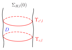
Figure 6.2. The region $D$ is bounded by two invariant circles

Then (6.2) and (6.10) together imply

$$\begin{split}|c_{1}-c_{1}^{\prime}|&=\left|\int_{D}\sum\limits_{i=1}^{2}dp_{i}\wedge dq_{i}\right|=\left|\int_{D}\left(1+\frac{\partial(\mathbf{p}_{2},\mathbf{q}_{2})}{\partial(p_{1},q_{1})}\right)dp_{1}\wedge dq_{1}\right|\\ &\geq\frac{1}{4}\left|\int_{D}dp_{1}\wedge dq_{1}\right|=\frac{1}{4}\left|\int_{\Upsilon_{c,l}}p_{1}dq_{1}-\int_{\Upsilon_{c^{\prime},l}}p_{1}dq_{1}\right|\\ &=\frac{1}{4}\left|\int_{\mathbb{T}}\pi_{p_{1}}\circ\Upsilon_{c,l}(q_{1})-\pi_{p_{1}}\circ\Upsilon_{c^{\prime},l}(q_{1})~{}dq_{1}\right|\end{split}$$ (6.11)

As the Lipschitz functions $\pi_{p_{1}}\circ\Upsilon_{c,l}$,   $\pi_{p_{1}}\circ\Upsilon_{c^{\prime},l}:\mathbb{T}\rightarrow\mathbb{R}$ satisfy $\pi_{p_{1}}\circ\Upsilon_{c^{\prime},l}>\pi_{p_{1}}\circ\Upsilon_{c,l}$, we have

$$\int_{\mathbb{T}}\pi_{p_{1}}\circ\Upsilon_{c^{\prime},l}(q_{1})-\pi_{p_{1}}\circ\Upsilon_{c,l}(q_{1})~{}dq_{1}\geq\frac{1}{4C_{L}}\left(\max\limits_{q_{1}}|\pi_{p_{1}}\circ\Upsilon_{c^{\prime},l}(q_{1})-\pi_{p_{1}}\circ\Upsilon_{c,l}(q_{1})|\right)^{2},$$ (6.12)

where $C_{L}$ is the Lipschitz bound of the functions $\pi_{p_{1}}\circ\Upsilon_{c,l}$ and $\pi_{p_{1}}\circ\Upsilon_{c^{\prime},l}$.

Recall that the function $\mathbf{p}_{2}(q_{1},p_{1})$ is at least $C^{1}$, then there exists a constant $K>0$ such that

$$\begin{split}&\|\pi_{p}\circ\Upsilon_{c,l}(q_{1})-\pi_{p}\circ\Upsilon_{c^{\prime},l}(q_{1})\|\\ =&|\pi_{p_{1}}\circ\Upsilon_{c,l}(q_{1})-\pi_{p_{1}}\circ\Upsilon_{c^{\prime},l}(q_{1})|+|\pi_{p_{2}}\circ\Upsilon_{c,l}(q_{1})-\pi_{p_{2}}\circ\Upsilon_{c^{\prime},l}(q_{1})|\\ =&|\pi_{p_{1}}\circ\Upsilon_{c,l}(q_{1})-\pi_{p_{1}}\circ\Upsilon_{c^{\prime},l}(q_{1})|+|\mathbf{p}_{2}(q_{1},\pi_{p_{1}}\circ\Upsilon_{c,l}(q_{1}))-\mathbf{p}_{2}(q_{1},\pi_{p_{1}}\circ\Upsilon_{c^{\prime},l}(q_{1}))|\\ \leq&(1+K)|\pi_{p_{1}}\circ\Upsilon_{c,l}(q_{1})-\pi_{p_{1}}\circ\Upsilon_{c^{\prime},l}(q_{1})|,\end{split}$$ (6.13)

Thus, combining (6.11), (6.12) with (6.13), one obtains

$$\begin{split}\|c-c^{\prime}\|&\geq|c_{1}-c_{1}^{\prime}|\geq\frac{1}{16C_{L}}\big{(}\max\limits_{q_{1}}|\pi_{p_{1}}\circ\Upsilon_{c,l}(q_{1})-\pi_{p_{1}}\circ\Upsilon_{c^{\prime},l}(q_{1})|\big{)}^{2}\\ &\geq\frac{1}{16C_{L}(1+K)^{2}}\big{(}\max\limits_{q_{1}}\|\pi_{p}\circ\Upsilon_{c,l}(q_{1})-\pi_{p}\circ\Upsilon_{c^{\prime},l}(q_{1})\|\big{)}^{2},\end{split}$$

which implies

$$\max\limits_{q_{1}}\|\pi_{p}\circ\Upsilon_{c,l}(q_{1})-\pi_{p}\circ\Upsilon_{c^{\prime},l}(q_{1})\|\leq 4\sqrt{C_{L}}(1+K)\|c-c^{\prime}\|^{\frac{1}{2}}.$$

Next, since the function $\mathbf{q}_{2}(q_{1},p_{1})$ is at least $C^{1}$, there exists a constant $\tilde{C}>0$ such that

$$\max\limits_{q_{1}}|\pi_{q_{2}}\circ\Upsilon_{c,l}(q_{1})-\pi_{q_{2}}\circ\Upsilon_{c^{\prime},l}(q_{1})| =\max\limits_{q_{1}}|\mathbf{q}_{2}(q_{1},\pi_{p_{1}}\circ\Upsilon_{c,l}(q_{1}))-\mathbf{q}_{2}(q_{1},\pi_{p_{1}}\circ\Upsilon_{c^{\prime},l}(q_{1}))$$

$$\leq\widetilde{C}\max\limits_{q_{1}}|\pi_{p_{1}}\circ\Upsilon_{c,l}(q_{1})-\pi_{p_{1}}\circ\Upsilon_{c^{\prime},l}(q_{1})|$$

$$\leq 4\sqrt{C_{L}}\widetilde{C}(1+K)\|c-c^{\prime}\|^{\frac{1}{2}}.$$

Consequently, item (1) follows immediately by setting $C=4\sqrt{C_{L}}(1+\widetilde{C})(1+K)$. ∎

We also mention that, for the Peierls barriers restricted on the NHIC, one can even obtain the Hölder continuity with respect to perturbations [18].

The result below is analogous to [25, Lemma 6.4] and will be crucial for the proof of genericity.

Theorem 6.6.

Let $\mathbf{r_{0}}$ be the constant given in Lemma 6.4, and we fix two points $z_{l}\in\mathrm{N}_{\mathbf{r_{0}},l},z_{u}\in\mathrm{N}_{\mathbf{r_{0}},u}$. Let $u^{\pm}_{c,l}(q,t)$, $u^{\pm}_{c,u}(q,t)$ be the elementary weak KAM solutions satisfying $u^{\pm}_{c,l}(z_{l},0)=u^{\pm}_{c,l}(z_{u},0)$ $\equiv\textup{constant}$, for all $c\in\mathbb{S}$. Then there exists $C_{h}>0$ such that for any $c,c^{\prime}\in\mathbb{S}$

$$|u^{\pm}_{c,l}(q,0)-u^{\pm}_{c^{\prime},l}(q,0)|\leq C_{h}(\|c^{\prime}-c\|^{\frac{1}{2}}+\|c^{\prime}-c\|),\quad\forall q\in\check{M}\setminus\mathrm{N}_{\mathbf{r_{0}},u}$$

and

$$|u^{\pm}_{c,u}(q,0)-u^{\pm}_{c^{\prime},u}(q,0)|\leq C_{h}(\|c^{\prime}-c\|^{\frac{1}{2}}+\|c^{\prime}-c\|),\quad\forall q\in\check{M}\setminus\mathrm{N}_{\mathbf{r_{0}},l}.$$

Remark.

By adding suitably constants, we can take $u^{\pm}_{c,l}(z_{l},0)=u^{\pm}_{c,l}(z_{u},0)=0$ for all $c\in\mathbb{S}$, since any elementary weak KAM solution plus a constant is still an elementary weak KAM solution.

Proof.

We only prove the case for $u^{-}_{c,l}$ and the others are similar. The normal hyperbolicity guarantees the smooth dependence of the unstable leaf $W_{q}^{u,loc}$ with respect to the base point $q\in\Sigma_{H,l}(0)$. By Lemma 6.5, the local unstable manifold $W^{u,loc}_{\Upsilon_{c,l}}$ of $\Upsilon_{c,l}$ is also $\frac{1}{2}-$Hölder continuous in $c\in\mathbb{S}$. Then, Lemma 6.4 implies that some constant $C_{1}>0$ exists such that

$$\|\big{(}c+\partial_{q}u_{c,l}^{-}(q,0)\big{)}-\big{(}c^{\prime}+\partial_{q}u_{c^{\prime},l}^{-}(q,0)\big{)}\|\leq C_{1}\|c-c^{\prime}\|^{\frac{1}{2}},~{}\forall q\in\mathrm{N}_{\mathbf{r_{0}},l},~{}\forall c,c^{\prime}\in\mathbb{S}.$$

Further, using integration we obtain that for all $c,c^{\prime}\in\mathbb{S}$ and all $q\in\mathrm{N}_{\mathbf{r_{0}},l}$,

$$\begin{split}\big{|}\big{(}u^{-}_{c,l}(q,0)-u^{-}_{c,l}(z_{l},0)+\langle c,q-z_{l}\rangle\big{)}-\big{(}u^{-}_{c^{\prime},l}(q,0)-u^{-}_{c^{\prime},l}(z_{l},0)+\langle c^{\prime},q-z_{l}\rangle\big{)}\big{|}\leq C_{1}\|c-c^{\prime}\|^{\frac{1}{2}}.\end{split}$$

Since we have chosen $u^{-}_{c,l}(z_{l},0)\equiv constant$ for all $c\in\mathbb{S}$, we get that $\forall$$c,c^{\prime}\in\mathbb{S}$ and $\forall q\in\mathrm{N}_{\mathbf{r_{0}},l}$

$$\begin{split}\big{|}u^{-}_{c,l}(q,0)-u^{-}_{c^{\prime},l}(q,0)\big{|}\leq C_{1}\|c-c^{\prime}\|^{\frac{1}{2}}+\|c-c^{\prime}\|.\end{split}$$ (6.14)

Next, for each $z\in\check{M}\setminus\mathrm{N}_{\mathbf{r_{0}},u}$, there exists a backward calibrated curve $\gamma^{-}_{c,l}$ with $\gamma_{c,l}^{-}(0)=z$, which is negatively asymptotic to $\pi_{q}\circ\Upsilon_{c,l}$. Since the duration of $\gamma^{-}_{c,l}$ staying outside $\mathrm{N}_{\mathbf{r_{0}},l}$ is uniformly bounded, denoted by $T_{l}\in\mathbb{Z}^{+}$, we have $\gamma^{-}_{c,l}(-k)\in\mathrm{N}_{\mathbf{r_{0}},l}$ for every integer $k\geq T_{l}$. Then,

$$u^{-}_{c,l}(\gamma^{-}_{c,l}(0),0)-u^{-}_{c,l}(\gamma^{-}_{c,l}(-T_{l}),-T_{l})=\int^{0}_{-T_{l}}L(\gamma^{-}_{c,l}(s),\dot{\gamma}^{-}_{c,l}(s),s)-\langle c,\dot{\gamma}^{-}_{c,l}(s)\rangle+\alpha(c)\,ds,$$

$$u^{-}_{c^{\prime},l}(\gamma^{-}_{c,l}(0),0)-u^{-}_{c^{\prime},l}(\gamma^{-}_{c,l}(-T_{l}),-T_{l})\leq\int^{0}_{-T_{l}}L(\gamma^{-}_{c,l}(s),\dot{\gamma}^{-}_{c,l}(s),s)-\langle c^{\prime},\dot{\gamma}^{-}_{c,l}(s)\rangle+\alpha(c^{\prime})\,ds.$$

Subtracting the first formula from the second one, one deduces from inequality (6.14) that

$$\begin{split}u^{-}_{c^{\prime},l}(z,0)-u^{-}_{c,l}(z,0)\leq&u^{-}_{c^{\prime},l}(\gamma^{-}_{c,l}(-T_{l}),-T_{l})-u^{-}_{c,l}(\gamma^{-}_{c,l}(-T_{l}),-T_{l})\\ &+\int^{0}_{-T_{l}}\langle c-c^{\prime},\dot{\gamma}^{-}_{c,l}(s)\rangle+\alpha(c^{\prime})-\alpha(c)\,ds\\ \leq&u^{-}_{c^{\prime},l}(\gamma^{-}_{c,l}(-T_{l}),0)-u^{-}_{c,l}(\gamma^{-}_{c,l}(-T_{l}),0)+C_{2}\|c^{\prime}-c\|\\ \leq&C_{1}\|c^{\prime}-c\|^{\frac{1}{2}}+\|c^{\prime}-c\|+C_{2}\|c^{\prime}-c\|.\end{split}$$

Here, the second inequality follows from the fact that $\|\dot{\gamma}^{-}_{c,l}\|$ is uniformly bounded and Mather’s $\alpha$-function is Lipschitz continuous. So we conclude that there exists $C_{h}>0$ such that

$$u^{-}_{c^{\prime},l}(z,0)-u^{-}_{c,l}(z,0)\leq C_{h}(\|c^{\prime}-c\|^{\frac{1}{2}}+\|c^{\prime}-c\|),~{}\forall z\in\check{M}\setminus\mathrm{N}_{\mathbf{r_{0}},u}.$$

In a similar way, we can prove that $u^{-}_{c,l}(z,0)-u^{-}_{c^{\prime},l}(z,0)$$\leq C_{h}(\|c^{\prime}-c\|^{\frac{1}{2}}+\|c^{\prime}-c\|)$ for all $z\in\check{M}\setminus\mathrm{N}_{\mathbf{r_{0}},u}$, which completes the proof. ∎

6.3. Choice of the Gevrey space

In what follows, we assume $\alpha>1$ and $M=\mathbb{T}^{2}$. As we will see later, our proof of genericity is not always valid for all Gevrey space $\mathbf{G}^{\alpha,\mathbf{L}}$ ($\mathbf{L}>0$), but only for $\mathbf{G}^{\alpha,\mathbf{L}}$ with $\mathbf{L}$ bounded by a positive constant $\mathbf{L}_{0}$. This is caused by Gevrey approximation, and we will explain it and show how to choose $\mathbf{L}_{0}$ below.

Let us first look at the unperturbed Lagrangian $L_{0}=l_{1}(v_{1})+l_{2}(q_{2},v_{2})$ in (1.3). For each $c=(c_{1},0)$, $|c_{1}|\leq R-1$, the Aubry set and Mañé set are

$$\widetilde{\mathcal{A}}_{L_{0}}(c,M)=\widetilde{\mathcal{N}}_{L_{0}}(c,M)=\{(q_{1},0,Dh_{1}(c_{1}),0,t)\in TM\times\mathbb{T}:q_{1}\in\mathbb{T},t\in\mathbb{T}\},$$

which is a $\phi_{L_{0}}^{1}$-invariant circle. Next, we work in the covering space $\check{M}$ and consider $L_{0}:T\check{M}\to\mathbb{R}$. Restricted on the time section $\{t=0\}$, the lift of the Aubry set has two copies:

$$\begin{split}\widetilde{\mathcal{A}}_{L_{0},l}(c,\check{M})|_{t=0}&=\{(q_{1},0,Dh_{1}(c_{1}),0)\in T\check{M}:q_{1}\in\mathbb{T}\},\\ \widetilde{\mathcal{A}}_{L_{0},u}(c,\check{M})|_{t=0}&=\{(q_{1},1,Dh_{1}(c_{1}),0)\in T\check{M}:q_{1}\in\mathbb{T}\},\end{split}$$

and they lie on the following two invariant cylinders respectively

$$\begin{split}\mathscr{L}\Sigma_{l}(0)=&\{(q_{1},0,Dh_{1}(p_{1}),0)\in T\check{M}:q_{1}\in\mathbb{T},|p_{1}|\leq R-1\},\\ \mathscr{L}\Sigma_{u}(0)=&\{(q_{1},1,Dh_{1}(p_{1}),0)\in T\check{M}:q_{1}\in\mathbb{T},|p_{1}|\leq R-1\}.\end{split}$$

Notice that $\pi_{q}\circ\mathscr{L}\Sigma_{l}(0)=\mathbb{T}\times\{0\}$ and $\pi_{q}\circ\mathscr{L}\Sigma_{u}(0)=\mathbb{T}\times\{1\}$.

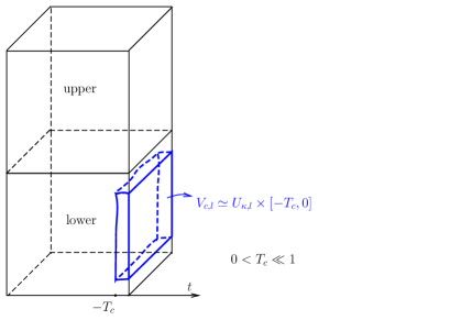
Figure 6.3. $V_{c,l}$ (blue) in a fundamental domain of $\check{M}\times\mathbb{T}$

Denote by $u^{\pm}_{c,l,L_{0}},u^{\pm}_{c,u,L_{0}}$ the elementary weak KAM solutions of $L_{0}$ with respect to the cohomology class $c$. Recall that $\kappa<\mathbf{r_{0}}$. For each $x\in\mathrm{U}_{\kappa,l}$, there exists a unique $u^{-}_{c,l,L_{0}}$-calibrated curve $\xi^{-}_{x,c}(t):(-\infty,0]\to\check{M}$ such that $\xi^{-}_{x,c}(0)=x$, and it is negatively asymptotic to $\mathcal{A}_{L_{0},l}(c)$. We pick and fix a constant $T_{c}=T_{c}(\kappa,L_{0})>0$ small enough, then we obtain a local neighborhood

$$V_{c,l}=\{(\xi_{x,c}^{-}(t),t)\in\check{M}\times\mathbb{T}:x\in\mathrm{U}_{\kappa,l},-T_{c}\leq t\leq 0\}$$

which is diffeomorphic to $\mathrm{U}_{\kappa,l}\times[-T_{c},0]$ (see figure 6.3), namely there is a diffeomorphism

$$f:\mathrm{U}_{\kappa,l}\times[-T_{c},0]\to V_{c,l}$$

such that $f(x,t)=(\xi^{-}_{x,c}(t),t)$ and $V_{c,l}\cap(\mathrm{N}_{3\kappa/4,l}\times\mathbb{T})=\emptyset$, this is guaranteed by $T_{c}\ll 1$. Notice that $V_{c,l}$ would vary in $c$.

Recall that $\check{M}=\mathbb{T}\times[0,2]/\sim$, where the equivalence relation $\sim$ is defined by identifying 0 with 2 in the $q_{2}$-coordinate. In the sequel, we will fix, once and for all, a sufficiently small constant $\delta>0$, which is smaller than $\kappa/4$. Thanks to Theorem 5.3 there exists a Gevrey-$(\alpha,\lambda_{c})$ diffeomorphism

$$\Psi_{c,l}:\mathrm{U}_{\kappa,l}\times[-T_{c},0]\to\text{\uj V}_{c,l}$$

such that $\|\Psi_{c,l}-f\|_{C^{0}(\mathrm{U}_{\kappa,l}\times[-T_{c},0])}\leq\delta/2$, where $\text{\uj V}_{c,l}\subsetneq\mathbb{T}\times(0,1)\times\mathbb{T}$ and $\text{\uj V}_{c,l}\cap(\mathrm{N}_{\kappa/2,l}\times\mathbb{T})=\emptyset$, $\lambda_{c}=\lambda_{c}(\kappa,L_{0})\ll 1$. It means that $\Psi_{c,l}(x,\cdot)$ remains $\delta/2-$close to $\xi^{-}_{x,c}(\cdot)$ in the following sense:

$$\textup{dist}(\Psi_{c,l}(x,t),\xi^{-}_{x,c}(t))\leq\delta/2,\quad\forall~{}(x,t)\in\mathrm{U}_{\kappa,l}\times[-T_{c},0].$$

Recall that the number $\varepsilon_{1}$ given in Lemma 6.3 is small enough, then one can find an small interval $I_{c}=\{(c^{\prime}_{1},0):c^{\prime}_{1}\in(c_{1}-\tau,c_{1}+\tau)\}$ depending on $\kappa,L_{0}$, such that if the perturbation term $\|L_{1}\|_{C^{2}}<2\varepsilon_{1}$, then the Lagrangian $L=L_{0}+L_{1}$ satisfies: for each $c^{\prime}\in I_{c}$, $x\in\mathrm{U}_{\kappa,l}$,

$\bullet$ the $u^{-}_{c^{\prime},l,L}$-calibrated curve $\gamma^{-}_{x,c^{\prime},L}(t):(-\infty,0]\to\check{M}$ with $\gamma^{-}_{x,c^{\prime},L}(0)=x$ is negatively asymptotic to $\mathcal{A}_{L,l}(c^{\prime},\check{M})$.

$\bullet$ $\gamma^{-}_{x,c^{\prime},L}(\cdot)$ is still $\delta-$close to $\Psi_{c,l}(x,\cdot)$ in the sense that

$$\textup{dist}(\Psi_{c,l}(x,t),\gamma^{-}_{x,c^{\prime},L}(t))\leq\delta,\quad\forall-T_{c}\leq t\leq 0.$$ (6.15)

These properties are guaranteed by the upper semi-continuity. By the finite covering theorem, there exist finitely many intervals $\{I_{c^{i}}\}_{i=0}^{m}$ such that

$$\bigcup_{0\leq i\leq m}I_{c^{i}}\supset[-R+1,R-1]\times\{0\},$$ (6.16)

and the corresponding diffeomorphism $\Psi_{c^{i},l}:\mathrm{U}_{\kappa,l}\times[-T_{c^{i}},0]\to\text{\uj V}_{c^{i},l}$ is Gevrey-$(\alpha,\lambda_{c^{i}})$, and the positive number $T_{c^{i}}\ll 1$. According to Theorem 5.2, some constant $\lambda^{\prime}_{c^{i}}<\lambda_{c^{i}}$ exists such that $\Psi_{c^{i},l}^{-1}$ is Gevrey-$(\alpha,\lambda^{\prime}_{c^{i}})$ smooth.

In what follows, we set

$$\mathbf{L}_{0}:=\min\{\lambda^{\prime}_{c^{i}}:i=0,\cdots,m\},$$ (6.17)

and hence

$$\Psi_{c^{i},l}^{-1}:\text{\uj V}_{c^{i},l}\to\mathrm{U}_{\kappa,l}\times[-T_{c^{i}},0]$$

is Gevrey-$(\alpha,\mathbf{L})$ smooth, for all $\mathbf{L}\leq\mathbf{L}_{0}$. We also point out that $\mathbf{L}_{0}$ is independent of the perturbation Hamiltonian $H_{1}$, and it depends only on $H_{0}$, $R$ and $\alpha$ since the choice of $\kappa$ depends only on $H_{0}$ and $R$, and $L_{0}$ depends only on $H_{0}$.

Similarly, these procedures can be carried out for the region $\mathrm{U}_{\kappa,u}$, and one can get the corresponding Gevrey diffeomorphism $\Psi_{c^{i},u}:\mathrm{U}_{\kappa,u}\times[-T_{c^{i}},0]\to\text{\uj V}_{c^{i},u}$. For simplicity, we still assume the same interval covering $\bigcup_{i=0}^{m}I_{c^{i}}$ as (6.16) and $\Psi_{c^{i},u}^{-1}:$$\text{\uj V}_{c^{i},u}\to\mathrm{U}_{\kappa,u}\times[-T_{c^{i}},0]$ is Gevrey-$(\alpha,\mathbf{L})$ smooth for all $\mathbf{L}\leq\mathbf{L}_{0}$, where each $\Psi_{c^{i},u}$ ($i=0,\cdots,m$) possesses the property analogous to (6.15).

6.4. Total disconnectedness

Let $\alpha>1$, we will study the topological structure of the set of minimal points for

$$B_{c,l,u}(x,\tau)=u^{-}_{c,l}(x,\tau)-u^{+}_{c,u}(x,\tau),\quad\text{and}\quad B_{c,u,l}(x,\tau)=u^{-}_{c,u}(x,\tau)-u^{+}_{c,l}(x,\tau)$$

defined in (3.5), where $u^{\pm}_{c,\imath}$ ($\imath=l,u$) are the elementary weak KAM solutions. Actually, we will show that the minimal set is totally disconnected for generic Lagrangian systems. Inspired by the technique in [20, Section 4.2], we will perturb directly a Lagrangian by small potential functions. Compared with the perturbative techniques used in [24, 25] which perturb the generating functions to create genericity, our technique in the current paper provides more information, we can prove the genericity not only in the usual sense but also in the sense of Mañé.

Let $L=L_{0}+L_{1}$ be our Lagrangian given in (1.3), where $\|L_{1}\|_{C^{2}}<\varepsilon_{1}$. Recall the interval covering $\bigcup_{0\leq i\leq m}I_{c^{i}}$ given in section 6.3, one can always suppose that the length of each interval $I_{c^{i}}$ is less than 1. Then Theorem 6.6 implies that for any $c,c^{\prime}\in I_{c^{i}}\cap\mathbb{S}$ and $q\in\mathrm{U}_{\kappa}=\mathrm{U}_{\kappa,l}\cup\mathrm{U}_{\kappa,u},$

$$\begin{split}|u^{\pm}_{c,l}(q,0)-u^{\pm}_{c^{\prime},l}(q,0)|\leq 2C_{h}\|c^{\prime}-c\|^{\frac{1}{2}},\qquad|u^{\pm}_{c,u}(q,0)-u^{\pm}_{c^{\prime},u}(q,0)|\leq 2C_{h}\|c^{\prime}-c\|^{\frac{1}{2}}.\end{split}$$ (6.18)

Fixing $\mathbf{L}\in(0,\mathbf{L}_{0}]$ and $\varepsilon_{0}\in(0,\varepsilon_{1})$, we consider the following set in $\mathbf{G}^{\alpha,\mathbf{L}}(M\times\mathbb{T})$ with $M=\mathbb{T}^{2}$:

$$\mathfrak{P}:=\{P\in\mathbf{G}^{\alpha,\mathbf{L}}(M\times\mathbb{T}):\|P\|_{\alpha,\mathbf{L}}<\varepsilon_{0},~{}\text{supp}P\cap(\check{\pi}\mathrm{N}_{\kappa/2}\times\mathbb{T})=\emptyset\}.$$ (6.19)

Then it is easily seen that each potential perturbation $P\in\mathfrak{P}$ to the Hamiltonian $H$ would not affect the NHIC since $\widetilde{\Sigma}_{H}\subset\check{\pi}\mathrm{N}_{\kappa/2}\times\mathbb{R}^{2}\times\mathbb{T}$, see (6.4). We also point out that, by a natural extension, any function in $\mathbf{G}^{\alpha,\mathbf{L}}(M\times\mathbb{T})$ can be viewed as a function defined on $\check{M}\times\mathbb{T}$.

Theorem 6.7.

Let $\alpha>1$, $\mathbf{L}\leq\mathbf{L}_{0}$. There exists a residual set $\mathcal{W}$$\subset\mathfrak{P}$ such that for each Gevrey potential function $P\in\mathcal{W}$, the Lagrangian $L+P:T\check{M}\times\mathbb{T}\to\mathbb{R}$ satisfies: for each $c\in\mathbb{S}$, the sets

$$\arg\min B_{c,l,u}\big{|}_{\mathrm{U}_{\kappa,l}\cup\mathrm{U}_{\kappa,u}},\quad\arg\min B_{c,u,l}\big{|}_{\mathrm{U}_{\kappa,l}\cup\mathrm{U}_{\kappa,u}}$$

are both totally disconnected. Here, $\arg\min B_{c,l,u}|_{\mathrm{U}_{\kappa,l}\cup\mathrm{U}_{\kappa,u}}$ stands for $\arg\min B_{c,l,u}\bigcap(\mathrm{U}_{\kappa,l}\cup\mathrm{U}_{\kappa,u})$, and $\arg\min B_{c,u,l}|_{\mathrm{U}_{\kappa,l}\cup\mathrm{U}_{\kappa,u}}$ stands for $\arg\min B_{c,l,u}\bigcap(\mathrm{U}_{\kappa,l}\cup\mathrm{U}_{\kappa,u})$.

Proof.

For $c\in\mathbb{S}$, we first study the set $\arg\min B_{c,l,u}$ restricted on the region $\mathrm{U}_{\kappa,l}\subset\check{M}\times\{t=0\}$. Let $\mathbf{r_{0}}>0$ be the constant give in Lemma 6.4. Recall that we have $\mathbf{r_{0}}>\kappa$. Then, to prove the total disconnectedness of $\arg\min B_{c,l,u}\big{|}_{\mathrm{U}_{\kappa,l}}$, it is enough to verify that

$$\textsf{the set~{}}\arg\min B_{c,l,u}\big{|}_{\bar{\mathrm{N}}_{\mathbf{r_{0}},l}\setminus\mathrm{N}_{\kappa,l}}\textsf{~{}is totally disconnected},$$ (6.20)

where ${\bar{\mathrm{N}}_{\mathbf{r_{0}},l}\setminus\mathrm{N}_{\kappa,l}}$ $\subset$ $\mathrm{U}_{\kappa,l}$ and $\bar{\mathrm{N}}_{\mathbf{r_{0}},l}$ is the closure of $\mathrm{N}_{\mathbf{r_{0}},l}$. To explain this, we recall that, according to Proposition 3.6, a point $(x,0)$ $\in$ $\arg\min B_{c,l,u}|_{\mathrm{U}_{\kappa,l}}$ if and only if there exists a $c$-semi static curve $\gamma_{x,c}:\mathbb{R}\to\check{M}$ with $\gamma_{x,c}(0)=x$, such that the orbit $\{\gamma_{x,c}(n):n\in\mathbb{Z}\}$ is negatively asymptotic to $\pi_{q}\circ\Upsilon_{c,l}$ and positively asymptotic to $\pi_{q}\circ\Upsilon_{c,u}$. Then, by letting $\kappa$ be suitably small if necessary, the orbit $\{\gamma_{x,c}(n):n\in\mathbb{Z}\}$ has to pass through the region ${\bar{\mathrm{N}}_{\mathbf{r_{0}},l}\setminus\mathrm{N}_{\kappa,l}}$ when it approaches $\pi_{q}\circ\Upsilon_{c,l}$, as a result of the normal hyperbolicity. Consequently, in what follows, we only need to check (6.20).

We first focus on the subinterval $I_{c^{0}}$ in the interval covering $\bigcup_{0\leq i\leq m}I_{c^{i}}$. Let us pick a $2$-dim disk

$$D=\{(x_{1},x_{2},t)\in\check{M}\times\mathbb{T}:~{}t=0,~{}|x_{1}-x_{1,0}|\leq d,~{}|x_{2}-x_{2,0}|\leq d\}\subset\bar{\mathrm{N}}_{\mathbf{r_{0}},l}\setminus\mathrm{N}_{\kappa,l}$$

which is centered at the point $(x_{1,0},x_{2,0})$, and $d$ is small. We also set

$$D+d_{1}:=\{(x_{1},x_{2},t)\in\check{M}\times\mathbb{T}:~{}t=0,~{}|x_{1}-x_{1,0}|\leq d+d_{1},~{}|x_{2}-x_{2,0}|\leq d+d_{1}\}\subset\bar{\mathrm{N}}_{\mathbf{r_{0}},l}\setminus\mathrm{N}_{\kappa,l}$$

with $0<d_{1}\ll 1$ (see figure 6.4).

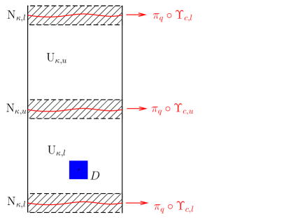
Figure 6.4. A fundamental domain of $\check{M}\times\{t=0\}$

Let $\mu$ be suitably small, for the index $i=1$ or $2$, we consider the following space

$$\mathfrak{V}_{i}:=\bigg{\{}\mu\Big{(}\sum\limits_{\ell=1,2}a_{i,\ell}\cos 2\ell\pi(x_{i}-x_{i,0})+b_{i,\ell}\sin 2\ell\pi(x_{i}-x_{i,0})\Big{)}~{}:~{}a_{i,\ell},b_{i,\ell}\in[1,2]\bigg{\}}.$$ (6.21)

Obviously, $\mathfrak{V}_{1},\mathfrak{V}_{2}\subset C^{\omega}(M)$. Next, we will construct perturbations based on potential functions of the form in $\mathfrak{V}_{i}$. To this end, we use the notation given in section 6.3. Fixing a sufficiently large constant $\mathfrak{L}\gg\mathbf{L}$, by Lemma 5.1 one can construct a function $\rho(x,t)=g(x)\chi(t):\check{M}\times\mathbb{T}\to\mathbb{R}$ such that $\chi:\mathbb{T}\to\mathbb{R}$ and $g(x):\check{M}\to\mathbb{R}$ are both non-negative Gevrey-$(\alpha,\mathfrak{L})$ functions. We choose

$$\chi(t)=\left\{\begin{array}[]{ll}>0,&~{}t\in(-T_{c^{0}},0)\\ =0,&~{}t\in\mathbb{T}\setminus(-T_{c^{0}},0)\end{array}\right.$$

where $T_{c^{0}}\ll 1$ is given in section 6.3, and require that $g|_{D}\equiv 1$ and supp$g\subset D+d_{1}$$\subset\bar{\mathrm{N}}_{\mathbf{r_{0}},l}\setminus\mathrm{N}_{\kappa,l}$. We set

$$\text{\uj C}:=\{\Psi_{c^{0},l}(x,t)~{}|~{}(x,t)\in(D+d_{1})\times[-T_{c^{0}},0]\},$$

then $\text{\uj C}\subset\text{\uj V}_{c^{0},l}\subsetneq\mathbb{T}\times(0,1)\times\mathbb{T}$, and therefore $\text{\uj C}\cap(\mathrm{N}_{\kappa/2,l}\times\mathbb{T})=\emptyset$.

$\bullet$ With each $V\in\mathfrak{V}_{1}$ or $\mathfrak{V}_{2}$, which can also be viewed as a function on $\check{M}$, one can define $\widetilde{V}\in C^{\infty}(\check{M}\times\mathbb{T})$ as follows: on the “lower” domain $\mathbb{T}\times[0,1]\times\mathbb{T}\subset\check{M}\times\mathbb{T}$,

$$\widetilde{V}(z)=\begin{cases}(\rho V)\circ\Psi_{c^{0},l}^{-1}(z)=\rho(x,t)V(x),&~{}\Psi_{c^{0},l}(x,t)=z\in\text{\uj C},\\ 0,&z\in(\mathbb{T}\times[0,1]\times\mathbb{T})\setminus\text{\uj C}.\end{cases}$$

Then we extend symmetrically the function to the “upper” domain $\mathbb{T}\times[1,2]\times\mathbb{T}$ such that

$$\widetilde{V}(y,t)=\widetilde{V}(y-\mathbf{e}_{2},t)$$

with $\mathbf{e}_{2}=(0,1).$ The support of $\widetilde{V}$ satisfies

$$\textup{supp}\widetilde{V}\subset\text{\uj C}\cup(\text{\uj C}+\mathbf{e}_{2}).$$ (6.22)

Since $\mathfrak{L}\gg\mathbf{L}$, according to the properties (G1), (G3) in Section 1, we have

$$\widetilde{V}\in\mathbf{G}^{\alpha,\mathbf{L}}(\check{M}\times\mathbb{T}).$$ (6.23)

$\bullet$ We also remark that, by the symmetry of $\widetilde{V}\in\mathbf{G}^{\alpha,\mathbf{L}}(\check{M}\times\mathbb{T})$, $\widetilde{V}$ can also be viewed as a function on $M\times\mathbb{T}$. By abuse of notation, we continue to write $\widetilde{V}\in\mathbf{G}^{\alpha,\mathbf{L}}(M\times\mathbb{T})$. Thus, $\widetilde{V}\in\mathfrak{P}.$ As a result of the construction above, some constant $C_{1}>0$ exists such that

$$\int_{-T_{c^{0}}}^{0}\widetilde{V}(\Psi_{c^{0},l}(x,t))dt=V(x)\int^{0}_{-T_{c^{0}}}g(x)\chi(t)dt=V(x)\int^{0}_{-T_{c^{0}}}\chi(t)dt=C_{1}V(x),\quad\text{for~{}}x\in D.$$ (6.24)

Here, we have used the fact $g|_{D}\equiv 1$.

Let $\Pi_{i}$, $i=1,2$, be the standard projection to the $i$-th coordinate of $\check{M}$. For the Lagrangian $L:T\check{M}\times\mathbb{T}\to\mathbb{R}$, we consider two elementary weak KAM solutions $u^{-}_{c,l}(q,t)$, $u^{+}_{c,u}(q,t)$, and denote by $u^{-}_{c,l,\widetilde{V}}(q,t)$, $u^{+}_{c,u,\widetilde{V}}(q,t)$ the elementary weak KAM solutions of the perturbed Lagrangian $L+\widetilde{V}$. Then the following result holds:

Lemma 6.8.

There exists an open and dense set $\mathcal{U}_{D}\subset\mathfrak{P}$ (see (6.19)) such that for each $\widetilde{V}\in\mathcal{U}_{D}$,

$$\Pi_{i}\left(\arg\min\big{(}u^{-}_{c,l,\widetilde{V}}(x,0)-u^{+}_{c,u,\widetilde{V}}(x,0)\big{)}\big{|}_{D}\right)\subsetneq[x_{i,0}-d,x_{i,0}+d],\quad\text{for all~{}}c\in I_{c^{0}}\cap\mathbb{S},$$ (6.25)

where $i=1,2$.

Proof.

We start with the perturbation $\widetilde{V}$ of the form (6.23), where $V\in\mathfrak{V}_{1}\cup\mathfrak{V}_{2}$. Note that under such a potential perturbation, the cylinders $\Sigma_{H,l}(0)$ and $\Sigma_{H,u}(0)$ remain unchanged, and hence the Aubry set $\widetilde{\mathcal{A}}_{L+\widetilde{V}}(c,\check{M})$ $=$ $\widetilde{\mathcal{A}}_{L}(c,\check{M})$.

Step 1: For $c\in I_{c^{0}}\cap\mathbb{S}$, the projected Aubry set $\mathcal{A}_{L}(c,\check{M})\subset\check{M}\times\mathbb{T}$ has two copies, denoted by $\mathcal{A}_{L,l}(c,\check{M})$ and $\mathcal{A}_{L,u}(c,\check{M})$. Each set $\mathcal{A}_{L,\imath}(c,\check{M})$, $\imath=l,u$ is diffeomorphic to $\mathbb{T}^{2}$ since $c\in\mathbb{S}$. For each $x\in D$ and each $u^{+}_{c,u}$-calibrated curve $\gamma^{+}_{x,c}(t):[0,+\infty)\to\check{M}$ with $\gamma^{+}_{x,c}(0)=x$, the minimizing curve $(\gamma^{+}_{x,c}(t),t):\mathbb{R}^{+}\longrightarrow\check{M}\times\mathbb{T}$ is positively asymptotic to $\mathcal{A}_{L,u}(c,\check{M})$. Now, we claim that

$$\textup{supp}\widetilde{V}~{}\bigcap~{}\big{(}\bigcup_{t>0}(\gamma^{+}_{x,c}(t),t)\big{)}=\emptyset,$$ (6.26)

as long as $D$ is small enough. In fact, according to (6.22), the support of $\tilde{V}$ has two copies in the lower and upper region respectively and $\textup{supp}\widetilde{V}\subset\text{\uj C}\cup(\text{\uj C}+\mathbf{e}_{2}).$ It is clear that the minimizing orbit $(\gamma^{+}_{x,c}(t),t)$ never intersects itself, then $\text{\uj C}\bigcap\big{(}\bigcup_{t>0}(\gamma^{+}_{x,c}(t),t)\big{)}=\emptyset$ since $D$ is a small neighborhood of $x$. Moreover, observe that the sets $\mathcal{A}_{L,l}(c,\check{M})$ and $\mathcal{A}_{L,u}(c,\check{M})$, which are diffeomorphic to $\mathbb{T}^{2}$, divide the $3$-dimensional configuration space $\check{M}\times\mathbb{T}$ into two connected components, then the minimizing curve $(\gamma^{+}_{x,c}(t),t):\mathbb{R}^{+}\longrightarrow\check{M}\times\mathbb{T}$ always stays in the lower region, which means $(\text{\uj C}+\mathbf{e}_{2})$ $\bigcap$ $\big{(}\bigcup_{t>0}(\gamma^{+}_{x,c}(t),t)\big{)}$ $=\emptyset$. This proves our claim (6.26). Consequently,

$$u^{+}_{c,u,\widetilde{V}}(x)=u^{+}_{c,u}(x),\quad\text{for all}~{}x\in D.$$ (6.27)

But the function $u^{-}_{c,l,\widetilde{V}}$ would undergo a small perturbation. Indeed, for $x\in D$, we can take a $u^{-}_{c,l,\widetilde{V}}$-calibrated curve $\gamma^{-}_{x,c,\widetilde{V}}:(-\infty,0]\to\check{M}$ with $\gamma^{-}_{x,c,\widetilde{V}}(0)=x$, then for $m\in\mathbb{Z}^{+}$,

$$u^{-}_{c,l,\widetilde{V}}(\gamma^{-}_{x,c,\widetilde{V}}(0),0)-u^{-}_{c,l,\widetilde{V}}(\gamma^{-}_{x,c,\widetilde{V}}(-m),-m)=\int_{-m}^{0}(L-\eta_{c}+\widetilde{V})(d\gamma^{-}_{x,c,\widetilde{V}}(t),t)+\alpha(c)\,dt,$$ (6.28)

For another perturbation $\widetilde{V}^{\prime}$, we have

$$u^{-}_{c,l,\widetilde{V}^{\prime}}(\gamma^{-}_{x,c,\widetilde{V}}(0),0)-u^{-}_{c,l,\widetilde{V}^{\prime}}(\gamma^{-}_{x,c,\widetilde{V}}(-m),-m)\leq\int_{-m}^{0}(L-\eta_{c}+\widetilde{V}^{\prime})(d\gamma^{-}_{x,c,\widetilde{V}}(t),t)+\alpha(c)\,dt.$$ (6.29)

By normal hyperbolicity, there exists a uniform upper bound $T\in\mathbb{Z}^{+}$, $T>T_{c^{0}}$, such that the orbit $\{(\gamma^{-}_{c,l,\widetilde{V}}(-t),t)\}_{t\geq T}$ shall retreat into the small neighborhood $\mathrm{N}_{\kappa/2,l}\times\mathbb{T}$. As the supports of $\widetilde{V}$ and $\widetilde{V}^{\prime}$ have empty intersection with $\mathrm{N}_{\kappa/2,l}\times\mathbb{T}$, we have $u^{-}_{c,l,\widetilde{V}}=u^{-}_{c,l,\widetilde{V}^{\prime}}$ on $\mathrm{N}_{\kappa/2,l}\times\mathbb{T}$. Then (6.28)-(6.29) imply that

$$u^{-}_{c,l,\widetilde{V}^{\prime}}(x,0)-u^{-}_{c,l,\widetilde{V}}(x,0)\leq\int_{-T}^{0}(\widetilde{V}^{\prime}-\widetilde{V})(\gamma^{-}_{x,c,\widetilde{V}}(t),t)\,dt.$$

Conversely, we can prove similarly that

$$u^{-}_{c,l,\widetilde{V}^{\prime}}(x,0)-u^{-}_{c,l,\widetilde{V}}(x,0)\geq\int_{-T}^{0}(\widetilde{V}^{\prime}-\widetilde{V})(\gamma^{-}_{x,c,\widetilde{V}^{\prime}}(t),t)\,dt,$$

where $\gamma^{-}_{x,c,\widetilde{V}^{\prime}}$ denotes the backward $u^{-}_{c,l,\widetilde{V}^{\prime}}$-calibrated curve with $\gamma^{-}_{x,c,\widetilde{V}^{\prime}}(0)=x$. Since $x$ lies in the region $D$ where $u^{-}_{c,l,\widetilde{V}}$ is differentiable (see Lemma 6.4), one has $\|\gamma^{-}_{x,c,\widetilde{V}^{\prime}}(t)-\gamma^{-}_{x,c,\widetilde{V}}(t)\|\to 0$ as $\|\widetilde{V}^{\prime}-\widetilde{V}\|\to 0$, which is guaranteed by the upper semi-continuity. Therefore, for $c\in I_{c^{0}}\cap\mathbb{S}$,

$$u^{-}_{c,l,\widetilde{V}^{\prime}}(x,0)-u^{-}_{c,l,\widetilde{V}}(x,0)=\mathscr{K}_{\widetilde{V},c}(\widetilde{V}^{\prime}-\widetilde{V})(x)+\mathscr{R}_{c}(\widetilde{V}^{\prime}-\widetilde{V})(x),\quad x\in D,$$ (6.30)

where the operator

$$\mathscr{K}_{\widetilde{V},c}(\widetilde{V}^{\prime}-\widetilde{V})(x)=\int_{-T}^{0}(\widetilde{V}^{\prime}-\widetilde{V})(\gamma_{x,c,\widetilde{V}}^{-}(t),t)\,dt,$$ (6.31)

and the remainder

$$\mathscr{R}_{c}(\widetilde{V}^{\prime}-\widetilde{V})=o(\|V^{\prime}-V\|_{C^{0}})$$

since $V,V^{\prime}\in\mathfrak{V}_{1}\cup\mathfrak{V}_{2}$ are linear combinations of trigonometric functions.

Step 2: Now, we claim that there exists an arbitrarily small perturbation $\widetilde{V}\in\mathfrak{P}$ of the form (6.23), such that

$$\Pi_{1}\left(\arg\min\big{(}u^{-}_{c,l,\widetilde{V}}(x,0)-u^{+}_{c,u,\widetilde{V}}(x,0)\big{)}\big{|}_{D}\right)\subsetneq[x_{1,0}-d,x_{1,0}+d],\quad\text{for all~{}}c\in I_{c^{0}}\cap\mathbb{S}.$$ (6.32)

To prove this claim, we construct a grid for the parameters $(a_{1,1},b_{1,1},a_{1,2},b_{1,2})$ in $\mathfrak{V}_{1}$ by splitting the domain $[1,2]^{4}$ equally into a family of 4-dimensional cubes whose side length is $\mu^{2}$, namely

$$\Delta a_{1,\ell}=\Delta b_{1,\ell}=\mu^{2},\quad\ell=1,2.$$

There are as many as $[\mu^{-8}]$ cubes.

In the sequel, we use the symbol $\textrm{Osc}_{x\in D}f$ to denote the oscillation of $f$, which describes the difference between the supremum and infimum of $f$ on $D$. According to (6.15), for each $c\in I_{c^{0}}\cap\mathbb{S}$ and $x\in D$, the backward $c$-semi static curve $\gamma^{-}_{x,c,\widetilde{V}}(t)$ will stay in the $\delta$-neighborhood of the curve $\Psi_{c^{0},l}(t)$ for $t\in[-T_{c^{0}},0]$ provided that $\mu$ is small enough. Besides, since minimizing orbits have no self intersections, by letting $D$ be suitably small if necessary, the minimizing curve $\big{(}\gamma^{-}_{x,c,\widetilde{V}}(t),t\big{)}:$ $[-T,-T_{c^{0}})$ $\longrightarrow$ $\check{M}\times\mathbb{T}$ does not intersect the support of $\widetilde{V}^{\prime}-\widetilde{V}$. This is guaranteed by using arguments similar to the proof of (6.26). Therefore, (6.24) and the above estimate imply that

$$\mathscr{K}_{\widetilde{V},c}(\widetilde{V}^{\prime}-\widetilde{V})(x)=\int_{-T_{c^{0}}}^{0}(\widetilde{V}^{\prime}-\widetilde{V})(\Psi_{c^{0},l}(x,t))\,dt+O(\mu\delta)=C_{1}(V^{\prime}(x)-V(x))+O(\mu\delta).$$ (6.33)

Then some constant $C_{2}>0$ exists such that

$$\text{Osc}_{x\in D}(\mathscr{K}_{\widetilde{V},c}(\widetilde{V}^{\prime}-\widetilde{V}))>\frac{1}{4}C_{1}\text{Osc}_{x\in D}(V-V^{\prime})>C_{2}\mu\Delta$$ (6.34)

where $\Delta=\max\{|a_{1,\ell}-a^{\prime}_{1,\ell}|,|b_{1,\ell}-b^{\prime}_{1,\ell}|:~{}\ell=1,2\}$. This is guaranteed by (6.33) and the fact that $V$ is a finitely linear combination of $\{\sin 2\pi x_{1},\cos 2\pi x_{1},\sin 4\pi x_{1},\cos 4\pi x_{1}\}$.

Next, we split the interval $I_{c^{0}}$ equally into $[K_{s}\mu^{-6}]$ subintervals, where $K_{s}=L_{s}(\frac{24C_{h}}{C_{2}})^{2}$ and $L_{s}$ is the length of $I_{c^{0}}$, $C_{h}$ is the constant given in (6.18) and $C_{2}$ is given in (6.34). We pick up the subinterval that has non-empty intersection with $\mathbb{S}$, and then denote all such kinds of subintervals by $\{\text{\uj J}_{i}\}_{i\in\mathbb{J}}$. Clearly, the cardinality of $\mathbb{J}$ is less than $[K_{s}\mu^{-6}]$.

Let us fix a $c^{*}\in\text{\uj J}_{i}\cap\mathbb{S}$. If for some parameter $(a^{*}_{1,\ell},b^{*}_{1,\ell}),\ell=1,2$ and its corresponding perturbation $V^{*}\in\mathfrak{V}_{1}$, formula (6.32) does not hold, then $\min_{x_{2}}\big{(}u^{-}_{c^{*},l,\widetilde{V}^{*}}(x,0)-u^{+}_{c^{*},u,\widetilde{V}^{*}}(x,0)\big{)}$ is identically equal to a constant for all $x\in D$, and hence

$$\textup{Osc}_{x\in D}\min\limits_{x_{2}}\big{(}u^{-}_{c^{*},l,\widetilde{V}^{*}}(x,0)-u^{+}_{c^{*},u,\widetilde{V}^{*}}(x,0)\big{)}=0.$$ (6.35)

Next, for another $V^{\prime}=\mu\Big{(}\sum_{\ell=1,2}a^{\prime}_{1,\ell}\cos 2\ell\pi(x_{1}-x_{1,0})+b^{\prime}_{1,\ell}\sin 2\ell\pi(x_{1}-x_{1,0})\Big{)}\in\mathfrak{V}_{1}$ and the corresponding perturbation $\widetilde{V}^{\prime}$, it follows from (6.27) and (6.30) that for all $c\in\text{\uj J}_{i}\cap\mathbb{S}$ and $x\in D$,

$$\begin{split}&\big{(}u^{-}_{c,l,\widetilde{V}^{\prime}}(x,0)-u^{+}_{c,u,\widetilde{V}^{\prime}}(x,0)\big{)}-\big{(}u^{-}_{c^{*},l,\widetilde{V}^{*}}(x,0)-u^{+}_{c^{*},u,\widetilde{V}^{*}}(x,0)\big{)}\\ =&\big{(}u^{-}_{c,l,\widetilde{V}^{\prime}}(x,0)-u^{-}_{c^{*},l,\widetilde{V}^{\prime}}(x,0)\big{)}-\big{(}u^{+}_{c,u,\widetilde{V}^{\prime}}(x,0)-u^{+}_{c^{*},u,\widetilde{V}^{\prime}}(x,0)\big{)}+\big{(}\mathscr{K}_{\widetilde{V}^{*},c^{*}}+\mathscr{R}_{c^{*}}\big{)}(\widetilde{V}^{\prime}-\widetilde{V}^{*})(x).\end{split}$$ (6.36)

As the length of $\text{\uj J}_{i}$ is $\frac{L_{s}}{[K_{s}\mu^{-}6]}$ and $c,c^{*}\in\text{\uj J}_{i}\cap\mathbb{S}$, formula (6.18) then implies that

$$\begin{split}&\Big{|}\big{(}u^{-}_{c,l,\widetilde{V}^{\prime}}(x,0)-u^{-}_{c^{*},l,\widetilde{V}^{\prime}}(x,0)\big{)}-\big{(}u^{+}_{c,u,\widetilde{V}^{\prime}}(x,0)-u^{+}_{c^{*},u,\widetilde{V}^{\prime}}(x,0)\Big{)}\big{|}\\ \leq&4C_{h}\|c-c^{*}\|^{\frac{1}{2}}\leq 4C_{h}\Big{(}\frac{L_{s}}{[K_{s}\mu^{-6}]}\Big{)}^{\frac{1}{2}}\leq\frac{C_{2}\mu^{3}}{6}.\end{split}$$ (6.37)

Since $\mu\ll 1$, one has $\|\widetilde{V}^{\prime}-\widetilde{V}^{*}\|\ll 1$ and

$$\|\mathscr{R}_{c^{*}}(\widetilde{V}^{\prime}-\widetilde{V}^{*})\|\leq\frac{1}{6}\|\mathscr{K}_{\widetilde{V}^{*},c^{*}}(\widetilde{V}^{\prime}-\widetilde{V}^{*})\|.$$ (6.38)

Regarding the potential function $V^{\prime}$, if its parameter $(a^{\prime}_{1,\ell},b^{\prime}_{1,\ell}),\ell=1,2$ satisfies

$$\max\{|a^{*}_{1,\ell}-a^{\prime}_{1,\ell}|,|b^{*}_{1,\ell}-a^{\prime}_{1,\ell}|:\ell=1,2\}\geq\mu^{2},$$ (6.39)

then inequalities (6.34)–(6.38) together give rise to

$$\textup{Osc}_{x\in D}\min\limits_{x_{2}}\big{(}u^{-}_{c,l,\widetilde{V}^{\prime}}(x,0)-u^{+}_{c,u,\widetilde{V}^{\prime}}(x,0)\big{)}\geq\frac{C_{2}}{3}\mu^{3}>0.$$

Thus we can conclude that for each $c\in\text{\uj J}_{i}\cap\mathbb{S}$ and $V^{\prime}\in\mathfrak{V}_{1}$ satisfying (6.39), we have

$$\begin{split}\textup{Osc}_{x\in D}\min\limits_{x_{2}}\big{(}u^{-}_{c,l,\widetilde{V}^{\prime}}(x,0)-u^{+}_{c,u,\widetilde{V}^{\prime}}(x,0)\big{)}>0.\end{split}$$ (6.40)

Consequently, for each $\text{\uj J}_{i}$, we only need to cancel out at most $2^{4}$ cubes from the grid $\{\Delta a_{1,\ell},\Delta b_{1,\ell}:\ell=1,2\}$ so that formula (6.40) holds for all other cubes. Let the index $i$ range over $\mathbb{J}$, we therefore obtain a set $\text{\uj P}_{1}\subseteq\{(a_{1,1},a_{1,2},b_{1,1},b_{1,2}):a_{1,\ell},b_{1,\ell}\in[1,2],\ell=1,2\}$ with Lebesgue measure

$$\textup{meas}\text{\uj P}_{1}\geq 1-2^{4}(\mu^{2})^{4}|\mathbb{J}|\geq 1-2^{4}K_{s}\mu^{2}>0,$$

such that formula (6.40) holds for any $V^{\prime}$ with parameter in $\text{\uj P}_{1}$ and any $c\in I_{c^{0}}\cap\mathbb{S}$. As $\mu$ is small enough, the claim (6.32) is now evident from what we have proved.

Step 3: Actually, the arguments above in Step 2 also ensure that formula (6.32) has density in $\mathfrak{P}$. The openness is obvious, so there is an open-dense set $\mathcal{U}_{D,1}$ in $\mathfrak{P}$ such that formula (6.32) holds for each perturbed Lagrangian $L+\tilde{V}$ with $\widetilde{V}\in\mathcal{U}_{D,1}$.

Analogously, we can consider a potential function $V\in\mathfrak{V}_{2}$ and its associated perturbation $\widetilde{V}$. By repeating similar arguments as in Step 2, we also obtain an open-dense set $\mathcal{U}_{D,2}\subset\mathfrak{P}$, such that for each perturbed Lagrangian $L+\tilde{V}$ where $\widetilde{V}\in\mathcal{U}_{D,2}$,

$$\Pi_{2}\left(\arg\min\big{(}u^{-}_{c,l,\widetilde{V}}(x,0)-u^{+}_{c,u,\widetilde{V}}(x,0)\big{)}\big{|}_{D}\right)\subsetneq[x_{2,0}-d,x_{2,0}+d],\quad\text{for all~{}}c\in I_{c^{0}}\cap\mathbb{S}.$$

Thus, the proof of Lemma 6.8 is now completed by taking a set $\mathcal{U}_{D}=\mathcal{U}_{D,1}\cap\mathcal{U}_{D,2}$. ∎

Now we continue to prove Theorem 6.7.

$\bullet$ From Lemma 6.8 we see that for each small disk $D\subseteq\bar{\mathrm{N}}_{\mathbf{r_{0}},l}\setminus\mathrm{N}_{\kappa,l}$, there exists an open-dense set $\mathcal{U}_{D}\subset\mathfrak{P}$ such that formula (6.25) holds for each Lagrangian $L+\widetilde{V}$ with $\widetilde{V}\in\mathcal{U}_{D}$. Next, we take a countable topology basis $\bigcup_{j}D_{j}$ for $\bar{\mathrm{N}}_{\mathbf{r_{0}},l}\setminus\mathrm{N}_{\kappa,l}$ where the diameter of $D_{j}$ approaches to $0$ as $j\to\infty$, and therefore obtain an open-dense set $\mathcal{U}_{D_{j}}$ for each $j$. Clearly, $\mathcal{U}_{I_{c^{0}}}=\bigcap_{j}\mathcal{U}_{D_{j}}$ is a residual set in $\mathfrak{P}$, and the set $\arg\min\big{(}u^{-}_{c,l,P}(x,0)-u^{+}_{c,u,P}(x,0)\big{)}\big{|}_{\bar{\mathrm{N}}_{\mathbf{r_{0}},l}\setminus\mathrm{N}_{\kappa,l}}$ is totally disconnected for each $P\in\mathcal{U}_{I_{c^{0}}}$ and $c\in\mathbb{S}\cap I_{c^{0}}$.

The technique above also works for other subintervals $I_{c^{i}},i=1,\cdots,m$, we can then obtain the corresponding residual sets $\mathcal{U}_{I_{c^{i}}},i=1,\cdots,m$. Hence the intersection $\mathcal{U}_{l}=\bigcap_{i=0}^{m}\mathcal{U}_{I_{c^{i}}}$ is residual, and $\arg\min\big{(}u^{-}_{c,l,P}(x,0)-u^{+}_{c,u,P}(x,0)\big{)}\big{|}_{\bar{\mathrm{N}}_{\mathbf{r_{0}},l}\setminus\mathrm{N}_{\kappa,l}}$ is totally disconnected for each $P\in\mathcal{U}_{l}$ and $c\in\mathbb{S}$. By what have shown at the beginning of the proof, this is equivalent to saying that $\arg\min\big{(}u^{-}_{c,l,P}(x,0)-u^{+}_{c,u,P}(x,0)\big{)}\big{|}_{\mathrm{U}_{\kappa,l}}$ is totally disconnected for each $P\in\mathcal{U}_{l}$ and $c\in\mathbb{S}$.

$\bullet$ Similarly, one can prove that there exists a residual set $\mathcal{U}_{u}\subset\mathfrak{P}$, such that the set

$$\arg\min\big{(}u^{-}_{c,l,P}(x,0)-u^{+}_{c,u,P}(x,0)\big{)}\big{|}_{\mathrm{U}_{\kappa,u}}$$

is totally disconnected for each $P\in\mathcal{U}_{u}$ and $c\in\mathbb{S}$.

$\bullet$ Conversely, by applying the technique above to $u^{-}_{c,u,P}(x,0)-u^{+}_{c,l,P}(x,0)$, we can also obtain two residual sets $\mathcal{V}_{l}$ and $\mathcal{V}_{u}$ in $\mathfrak{P}$, such that the set $\arg\min\big{(}u^{-}_{c,u,P}(x,0)-u^{+}_{c,l,P}(x,0)\big{)}\big{|}_{\mathrm{U}_{\kappa,l}}$ is totally disconnected for each $c\in\mathbb{S}$ and $P\in\mathcal{V}_{l}$, and the set $\arg\min\big{(}u^{-}_{c,u,P}(x,0)-u^{+}_{c,l,P}(x,0)\big{)}\big{|}_{\mathrm{U}_{\kappa,u}}$ is totally disconnected for each $c\in\mathbb{S}$ and $P\in\mathcal{V}_{u}$.

Therefore, the proof of Theorem 6.7 is now completed by taking $\mathcal{W}=\mathcal{U}_{l}\cap\mathcal{U}_{u}\cap\mathcal{V}_{l}\cap\mathcal{V}_{u}$. ∎

6.5. Proof of Theorem 1.2 and 1.3

Now, we are able to prove our main results. Let $R>1$, $\alpha>1$ and $0<\mathbf{L}\leq\mathbf{L}_{0}=\mathbf{L}_{0}(H_{0},\alpha,R)$, where the constant $\mathbf{L}_{0}$ is given in (6.17) and independent of $H_{1}$.

Proof.

In our problem $M=\mathbb{T}^{2}$, $s>0$, $y_{\ell}\in[-R+1,R-1]\times\{0\}$, $\ell\in\{1,\cdots,k\}$. Let $\varepsilon_{0}$ be a small positive number satisfying

$$\varepsilon_{0}<\min\{1,\mathbf{L}^{\alpha},\frac{\mathbf{L}^{2\alpha}}{2!^{\alpha}},\frac{\mathbf{L}^{3\alpha}}{3!^{\alpha}}\}\varepsilon_{1},$$

where $\varepsilon_{1}$ is chosen as in Lemma 6.3. Now, $\|H_{1}\|_{\alpha,\mathbf{L}}<\varepsilon_{0}$ implies $\|H_{1}\|_{C^{3}}<\varepsilon_{1}$, and hence the Hamiltonian $H=H_{0}+H_{1}$ has a persistent normally hyperbolic invariant cylinder (NHIC), and the globally minimal set $\widetilde{\mathcal{G}}_{L}(c)$ lies in this NHIC for each $c=(c_{1},0)$ with $|c_{1}|\leq R-1$. Here, $L=L_{0}+L_{1}$ is the Lagrangian associated to $H=H_{0}+H_{1}$. Also, observe that for the Mañé set $\widetilde{\mathcal{N}}_{L_{0}}(c)$,

$$\pi_{p}\circ\mathscr{L}^{-1}\widetilde{\mathcal{N}}_{L_{0}}(c)=c,\quad\text{~{}for each~{}}c=(c_{1},0),|c_{1}|\leq R-1.$$ (6.41)

By letting $\varepsilon_{0}$ be small enough, the perturbation term $L_{1}$ is also sufficiently small, then the upper semi-continuity (see Proposition 2.1) implies that for each $c=(c_{1},0)$, $|c_{1}|\leq R-1$,

$$d(\pi_{p}\circ\mathscr{L}^{-1}\widetilde{\mathcal{N}}_{L}(c),\pi_{p}\circ\mathscr{L}^{-1}\widetilde{\mathcal{N}}_{L_{0}}(c))<s/2,\quad\text{whenever~{}}\|H_{1}\|_{\alpha,\mathbf{L}}<\varepsilon_{0}$$ (6.42)

With this fact, one can find that $\varepsilon_{0}=\varepsilon_{0}(H_{0},\alpha,R,s,\mathbf{L})>0$ depends on the Hamiltonian $H_{0}$ and the constants $\alpha$, $R$, $\mathbf{L}$ and $s$.

Density: For each Hamiltonian $H_{0}+H_{1}$ with $\|H_{1}\|_{\alpha,\mathbf{L}}<\varepsilon_{0},$ we will prove that there exists an arbitrarily small perturbation $V\in\mathbf{G}^{\alpha,\mathbf{L}}(M\times\mathbb{T})$ such that $\|H_{1}+V\|_{\alpha,\mathbf{L}}<\varepsilon_{0}$, and the perturbed Hamiltonian $H_{0}+H_{1}+V$ has an orbit $(q(t),p(t))$ and times $t_{1}<\cdots<t_{k}$ such that the action variables $p(t)$ pass through the ball $B_{s}(y_{\ell})$ at the time $t=t_{\ell}$. To this end, we will establish a generalized transition chain along which one is able to apply Theorem 4.3.

Let $d\in(0,\varepsilon_{0}-\|H_{1}\|_{\alpha,\mathbf{L}})$ be arbitrarily small.

$\bullet$ First, by applying the genericity property in Corollary 6.2 to the Tonelli Lagrangian $L_{0}+L_{1}$, one can always choose a small perturbation

$$\phi\in\mathbf{G}^{\alpha,\mathbf{L}}(M\times\mathbb{T}),\quad\|\phi\|_{\alpha,\mathbf{L}}<\frac{d}{2}$$

such that for each rational homology class $h=(\frac{p}{q},0)$, the perturbed Lagrangian $L_{0}+L_{1}+\phi$ has only one minimal measure with the rotation vector $h$. Next, for the irrational case, it is well known in Aubry-Mather theory that for homology $h=(h_{1},0)$ with $h_{1}\in\mathbb{R}\setminus\mathbb{Q}$, only one minimal measure with the rotation vector $h$ exists. Thus it is easily seen that the Aubry class is unique for each $c=(c_{1},0)$ with $|c_{1}|\leq R-1$, as a result of property (2.1). Then the uniqueness of Aubry class implies

$$\widetilde{\mathcal{A}}_{L_{0}+L_{1}+\phi}(c)=\widetilde{\mathcal{N}}_{L_{0}+L_{1}+\phi}(c).$$ (6.43)

By the Legendre transformation, the associated Hamiltonian is exactly $H_{0}+H_{1}-\phi$ with $\|H_{1}-\phi\|_{\alpha,\mathbf{L}}<\varepsilon_{0}$, so (6.42) and (6.43) imply that

$$\pi_{p}\circ\mathscr{L}^{-1}\widetilde{\mathcal{A}}_{L_{0}}(c)=c,\quad d\left(\pi_{p}\circ\mathscr{L}^{-1}\widetilde{\mathcal{A}}_{L_{0}+L_{1}+\phi}(c),~{}\pi_{p}\circ\mathscr{L}^{-1}\widetilde{\mathcal{A}}_{L_{0}}(c)\right)<s/2,$$ (6.44)

for each $c=(c_{1},0)$, $|c_{1}|\leq R-1$.

Recall that the set $\widetilde{\mathcal{N}}_{L_{0}+L_{1}+\phi}(c)\big{|}_{t=0}$ lies in the NHIC, so it is either homologically trivial or not. In the homologically trivial case, it is well known that the $c$-equivalence holds inside $(c_{1}-\delta_{c},c_{1}+\delta_{c})\times\{0\}$ for some small $\delta_{c}>0$, which satisfies condition (1) in Definition 4.2.

In the latter case, $\widetilde{\mathcal{N}}_{L_{0}+L_{1}+\phi}(c)\big{|}_{t=0}$ must be an invariant curve as a result of (6.43). Then we define as (6.5) the set

$$\mathbb{S}:=\{(c_{1},0)~{}:~{}|c_{1}|\leq R-1,\Upsilon_{c}\textup{~{}is an invariant circle on the NHIC}\}.$$

Applying Theorem 6.7 to $L_{0}+L_{1}+\phi$, we can find a small potential perturbation with compact support

$$P\in\mathbf{G}^{\alpha,\mathbf{L}}(M\times\mathbb{T}),\quad\|P\|_{\alpha,\mathbf{L}}<\frac{d}{2},$$

such that the Lagrangian $L_{0}+L_{1}+\phi+P:T\check{M}\times\mathbb{T}\to\mathbb{R}$, defined in the double covering space, satisfies: for all $c\in\mathbb{S}$, the sets

$$\arg\min B_{c,l,u}\big{|}_{\mathrm{U}_{\kappa,l}\cup\mathrm{U}_{\kappa,u}},\quad\arg\min B_{c,u,l}\big{|}_{\mathrm{U}_{\kappa,l}\cup\mathrm{U}_{\kappa,u}}$$

are both totally disconnected. Then Proposition 3.5 and 3.6 together yield that for each $c\in\mathbb{S}$, there exists a small $\delta_{c}>0$ such that the set

$$\check{\pi}\mathcal{N}(c,\check{M})\big{|}_{t=0}\setminus(\mathcal{A}(c,M)\big{|}_{t=0}+\delta_{c})$$

is totally disconnected, which satisfies condition (2) in Definition 4.2. Consequently, the corresponding Hamiltonian is exactly $H_{0}+H_{1}-\phi-P$ where $\|\phi+P\|_{\alpha,\mathbf{L}}<d$ and $\|H_{1}-\phi-P\|_{\alpha,\mathbf{L}}<\varepsilon_{0}$.

$\bullet$ Next, we take

$$V=-\phi-P.$$

Then the arguments above imply that there exists a generalized transition chain inside $[-R+1,R-1]\times\{0\}$$\subset H^{1}(M,\mathbb{R})$ for the Lagrangian $L_{0}+L_{1}-V$. Thus, we conclude from Theorem 4.3 and (6.44) that the perturbed Hamiltonian $H_{0}+H_{1}+V$ has an orbit $(q(t),p(t))$ whose action variables $p(t)$ pass through the ball $B_{s}(y_{\ell})$ at the time $t=t_{\ell}$, where $t_{1}<t_{2}<\cdots<t_{k}$. Finally, thanks to $\|V\|_{\alpha,\mathbf{L}}<d$ and the arbitrariness of $d$, we complete the proof of density in $\mathfrak{B}^{\mathbf{L}}_{\varepsilon_{0},R}$.

Openness: It only remains to verify the openness. Since the time for the aforementioned trajectory $(q(t),p(t))$ passing through the balls $B_{s}(y_{1})$, $\cdots$, $B_{s}(y_{k})$ is finite, the smooth dependence of solutions of ODEs on parameters can guarantee the openness in $\mathfrak{B}^{\mathbf{L}}_{\varepsilon_{0},R}$. Theorem 1.2 is now evident from what we have proved.

Notice that in the proof of density part above, the perturbation we constructed is Gevrey potential function. Combining with the obvious openness property, Theorem 1.3 is also true. ∎

Appendix A Normally hyperbolic theory

In this appendix, we review some classical results in the theory of normally hyperbolic manifolds. We only give a less general introduction which is better applied to our problem, and refer the reader to [40, 41, 50, 71] for the proofs and more detailed introductions.

Definition A.1.

Let $M$ be a smooth Riemannian manifold and $f:M\to M$ be a $C^{r}(r\geq 1)$ diffeomorphism. Let $N\subset M$ be a submanifold (probably with boundary) which is invariant under $f$. Then $N$ is called a normally hyperbolic invariant manifold (NHIM) if there is an $f$-invariant tangent bundle splitting such that, for every $x\in N$

$$T_{x}M=T_{x}N\oplus E_{x}^{s}\oplus E_{x}^{u},$$

and there exist a constant $C>0$, rates $0<\lambda<1<\mu$ with $\lambda\mu<1$ such that

$$\begin{split}v\in T_{x}N&\Longleftrightarrow\|Df^{k}(x)v\|\leq C\mu^{|k|}\|v\|,\quad k\in\mathbb{Z},\\ v\in E^{s}_{x}&\Longleftrightarrow\|Df^{k}(x)v\|\leq C\lambda^{k}\|v\|,\quad k\geq 0,\\ v\in E^{u}_{x}&\Longleftrightarrow\|Df^{k}(x)v\|\leq C\lambda^{|k|}\|v\|,\quad k\leq 0.\\ \end{split}$$ (A.1)

In what follows, $N$ is assumed to be compact and connected. Let $U$ be a tubular neighborhood of the NHIM $N$. In both [40] and [50] the existence of local stable and unstable manifolds in $U$, denoted by $W_{N}^{s,loc}$ and $W_{N}^{u,loc}$ respectively, are obtained by using the method of Hadamards graph transform. Moreover, the local stable and unstable manifolds can be characterized as follows:

$$\begin{split}W_{N}^{s,loc}&=\{y\in U~{}|~{}\textup{dist}(f^{k}(y),N)\leq\tilde{C}_{y}(\lambda+\tilde{\varepsilon})^{k},\textup{~{}for all~{}}k\geq 0\},\\ W_{N}^{u,loc}&=\{y\in U~{}|~{}\textup{dist}(f^{k}(y),N)\leq\tilde{C}_{y}(\lambda+\tilde{\varepsilon})^{|k|},\textup{~{}for all~{}}k\leq 0\},\end{split}$$ (A.2)

where the constant $\tilde{C}_{y}>0$, and $\tilde{\varepsilon}>0$ is a small constant satisfying $\lambda+\tilde{\varepsilon}<1/\mu$. For each $x\in N$, the corresponding local stable and unstable leaves are defined as follows:

$$\begin{split}W_{x}^{s,loc}&=\{y\in U~{}|~{}\textup{dist}(f^{k}(x),f^{k}(y))\leq\tilde{C}_{x,y}(\lambda+\tilde{\varepsilon})^{k},\textup{~{}for all~{}}k\geq 0\},\\ W_{x}^{u,loc}&=\{y\in U~{}|~{}\textup{dist}(f^{k}(x),f^{k}(y))\leq\tilde{C}_{x,y}(\lambda+\tilde{\varepsilon})^{|k|},\textup{~{}for all~{}}k\leq 0\}.\end{split}$$ (A.3)

where $\tilde{C}_{x,y}>0$ is a constant. Then we have the following properties (see [50]):

Theorem A.2.

Let $N$ be a NHIM given in (A.1), and we define an integer $l:=\max\{k\in\mathbb{Z}~{}|~{}1\leq k\leq r$ $\text{~{}and~{}}k<\frac{|\log\lambda|}{\log\mu}\}$, then

1. $N$, $W_{N}^{s,loc}$ and $W_{N}^{u,loc}$ are $C^{l}$ manifolds. For each $x\in N$, the manifolds $W_{x}^{s,loc}$ and $W_{x}^{u,loc}$ are $C^{r}$ and $T_{x}W_{x}^{s,loc}=E_{x}^{s}$, $T_{x}W_{x}^{u,loc}=E_{x}^{u}$.

2. $W_{N}^{s,loc}$ and $W_{N}^{u,loc}$ are foliated by the stable and unstable leaves respectively, i.e.

   $$W_{N}^{s,loc}=\bigcup_{x\in N}W_{x}^{s,loc},\quad W_{N}^{u,loc}=\bigcup_{x\in N}W_{x}^{u,loc}.$$

   Moreover, if $x\neq x^{\prime}$, then $W_{x}^{s,loc}\bigcap W_{x^{\prime}}^{s,loc}=\emptyset$ and $W_{x}^{u,loc}\bigcap W_{x^{\prime}}^{u,loc}=\emptyset.$

3. The unstable foliation $\{W^{u,loc}_{x}:x\in N\}$ is $C^{l}$ in the sense that $\bigcup_{x\in N}T^{k}_{x}W^{u,loc}_{x}$ is a continuous bundle for each $1\leq k\leq l$, where $T^{k}$ denotes the $k$-th order tangent. Analogous result holds for the stable foliation.

Remark.

(1): We point out that for the models studied in the current paper, we have smoothness as high as the time-$1$ map since the dynamics on $N$ is close to integrable.
(2): We can also define the global stable (unstable) sets $W_{N}^{s,u}$ and $W_{x}^{s,u}$, just by replacing $U$ with $M$ in (A.2), (A.3). But $W_{N}^{s,u},W_{x}^{s,u}$ may fail to be embedded manifolds.

The normal hyperbolicity has stability under perturbations. Roughly speaking, the normally hyperbolic invariant manifold persists under small perturbations.

Theorem A.3 (Persistence of normally hyperbolic invariant manifolds).

Suppose that $N\subset M$ is a NHIM for the $C^{r}$ $(r\geq 1)$ diffeomorphism $f$ and $\varepsilon>0$ is sufficiently small. Then for any $C^{r}$ diffeomorphism $f_{\varepsilon}:M\to M$ satisfying $\|f_{\varepsilon}-f\|_{C^{1}}<\varepsilon$, there exists a NHIM $N_{\varepsilon}$ that is $C^{l}$ diffeomorphic and close to $N$ where $l=\max\{k:1\leq k\leq r$ $\text{~{}and~{}}k<\frac{|\log\lambda|}{\log\mu}\}$. Moreover, the local stable manifold $W^{s,loc}_{N_{\varepsilon}}$ and local unstable manifold $W^{u,loc}_{N_{\varepsilon}}$ are $C^{l}$ close to those of $N$.

Appendix B Variational construction of global connecting orbits

The goal of this section is to prove Theorem 4.3, which could be achieved by modifying the arguments and techniques in [25]. We also refer the reader to [21] or [19] for more details. Throughout this section, we assume $M=\mathbb{T}^{n}$. Our diffusing orbits are constructed by shadowing a sequence of local connecting orbits, along each of them the Lagrangian action attains a “local minimum”.

B.1. Local connecting orbits

Let $d\gamma(t)=(\gamma(t),\dot{\gamma}(t))$. An orbit $(d\gamma(t),t):\mathbb{R}\to TM\times\mathbb{T}$ is said to connect one Aubry set $\widetilde{\mathcal{A}}(c)$ to another one $\widetilde{\mathcal{A}}(c^{\prime})$ if the $\alpha$-limit set of the orbit is contained in $\widetilde{\mathcal{A}}(c)$ and the $\omega$-limit set is contained in $\widetilde{\mathcal{A}}(c^{\prime})$. We will introduce two types of local connecting orbits: type-$c$ and type-$h$, the former corresponds to Mather’s cohomology equivalence, while the latter corresponds to the variational interpretation of Arnold’s mechanism. Before that, we need some preparations.

B.1.1. Time-step Lagrangian and upper semi-continuity

Both types of local connecting orbits depend on the upper semi-continuity of minimal curves of a modified $C^{r}$ Lagrangian $L^{*}:T\mathbb{T}^{n}\times\mathbb{R}\rightarrow\mathbb{R}$ which is defined as follows: let $L^{+},L^{-}$ be two time-1 periodic Tonelli Lagrangians,

$$L^{*}(\cdot,t):=\begin{cases}L^{-}(\cdot,t),&~{}t\in(-\infty,0]\\ L^{+}(\cdot,t),&~{}t\in[1,+\infty),\end{cases}$$

and $L^{*}$ is superlinear and positive definite in the fibers. Notice that $L^{*}$ is not periodic in time $t$, instead, it is periodic when restricted on either $(-\infty,0]$ or $[1,+\infty)$. We call such a modified Lagrangian $L^{*}$ a time-step Lagrangian.

For a time-step Lagrangian $L^{*}$, a curve $\gamma:\mathbb{R}\rightarrow\mathbb{T}^{n}$ is called minimal if for any $t<t^{\prime}\in\mathbb{R}$,

$$\int_{t}^{t^{\prime}}L^{*}(\gamma(s),\dot{\gamma}(s),s)\,ds=\min\limits_{\begin{subarray}{c}\zeta(t)=\gamma(t),\zeta(t^{\prime})=\gamma(t^{\prime})\\ \zeta\in C^{ac}([t,t^{\prime}],\mathbb{T}^{n})\end{subarray}}\int_{t}^{t^{\prime}}L^{*}(\zeta(s),\dot{\zeta}(s),s)\,ds$$

Hence, we denote by $\mathscr{G}(L^{*})$ the set of all minimal curves and $\widetilde{\mathscr{G}}(L^{*})=\bigcup_{\gamma\in\mathscr{G}(L^{*})}(\gamma(t),\dot{\gamma}(t),t)$.

Let $\alpha^{\pm}$ denote Mather’s minimal average action of $L^{\pm}$. For $m_{0},m_{1}\in\mathbb{T}^{n}$ and $T_{0},T_{1}\in\mathbb{Z}_{+}$, we define

$$h^{T_{0},T_{1}}_{L^{*}}(m_{0},m_{1}):=\inf\limits_{\begin{subarray}{c}\gamma(-T_{0})=m_{0},\gamma(T_{1})=m_{1}\\ \gamma\in C^{ac}([-T_{0},T_{1}],\mathbb{T}^{n})\end{subarray}}\int_{-T_{0}}^{T_{1}}L^{*}(\gamma(t),\dot{\gamma}(t),t)\,dt+T_{0}\alpha^{-}+T_{1}\alpha^{+},$$

and

$$h_{L^{*}}^{\infty}(m_{0},m_{1}):=\liminf_{T_{0},T_{1}\to+\infty}h_{L^{*}}^{T_{0},T_{1}}(m_{0},m_{1}),$$

which are bounded. We take any two sequences of positive integers $\{T_{0}^{i}\}_{i\in\mathbb{Z}_{+}}$ and $\{T_{1}^{i}\}_{i\in\mathbb{Z}_{+}}$ with $T_{\ell}^{i}\rightarrow+\infty$ ($\ell=0,1$) as $i\to+\infty$ and the associated minimal curve $\gamma_{i}(t)$: $[-T^{i}_{0},T^{i}_{1}]\to\mathbb{T}^{n}$ connecting $m_{0}$ to $m_{1}$ such that

$$h_{L^{*}}^{\infty}(m_{0},m_{1})=\lim_{i\to\infty}h_{L^{*}}^{T_{0}^{i},T_{1}^{i}}(m_{0},m_{1})=\lim_{i\to\infty}\int_{-T_{0}^{i}}^{T_{1}^{i}}L^{*}(\gamma_{i}(t),\dot{\gamma}_{i}(t),t)\,dt+T^{i}_{0}\alpha^{-}+T^{i}_{1}\alpha^{+}.$$

The following lemma shows that any accumulation point $\gamma$ of $\{\gamma_{i}\}_{i}$ is a pseudo curve playing an analogous role as a semi-static curve. For the proof, see [24] or [25].

Lemma B.1.

Let $\gamma$: $\mathbb{R}\to\mathbb{T}^{n}$ be an accumulation point of $\{\gamma_{i}\}_{i}$ as shown above. Then for any $s\geq 0$, $t\geq 1$,

$$\begin{split}\int_{-s}^{t}L^{*}(\gamma(\tau),\dot{\gamma}(\tau),\tau)\,d\tau+s\alpha^{-}+t\alpha^{+}=\inf\limits_{\begin{subarray}{c}\xi(-s_{1})=\gamma(-s)\\ \xi(t_{1})=\gamma(t)\\ s_{1}-s\in\mathbb{Z},~{}t_{1}-t\in\mathbb{Z}\\ s_{1}\geq 0,~{}t_{1}\geq 1\end{subarray}}\int_{-s_{1}}^{t_{1}}L^{*}(\xi(\tau),\dot{\xi}(\tau),\tau)\,d\tau+s_{1}\alpha^{-}+t_{1}\alpha^{+},\end{split}$$ (B.1)

where the minimum is taken over all absolutely continuous curves.

This leads us to define the set of pseudo connecting curves

$$\mathscr{C}(L^{*}):=\{\gamma|~{}\gamma\in\mathscr{G}(L^{*})\text{~{}and~{}}\eqref{pseudo curve formula}\text{~{}holds}\}.$$

Clearly, for each $\gamma\in\mathscr{C}(L^{*})$ the orbit $(\gamma(t),\dot{\gamma}(t),t)$ would negatively approach the Aubry set $\widetilde{\mathcal{A}}(L^{-})$ of the Lagrangian $L^{-}$ and positively approach the Aubry set $\widetilde{\mathcal{A}}(L^{+})$ of $L^{+}$. This is why we call it a pseudo connecting curve. Define the following sets

$$\widetilde{\mathcal{C}}(L^{*}):=\bigcup_{\gamma\in\mathscr{C}(L^{*})}(\gamma(t),\dot{\gamma}(t),t),\qquad\mathcal{C}(L^{*}):=\bigcup_{\gamma\in\mathscr{C}(L^{*})}(\gamma(t),t).$$

Notice that if $L^{*}$ is time-1 periodic, then $\widetilde{\mathcal{C}}(L^{*})$ is exactly the Mañé set and $\mathcal{C}(L^{*})$ is exactly the projected Mañé set. Then we can prove the following property:

Proposition B.2.

The set-valued map $L^{*}\mapsto\mathscr{C}(L^{*})$ is upper semi-continuous, namely if $L^{*}_{i}\to L^{*}$ in the $C^{2}$ topology, then we have the set inclusion

$$\limsup_{i}\mathscr{C}(L^{*}_{i})\subset\mathscr{C}(L^{*}).$$

Consequently, the map $L^{*}\mapsto\widetilde{\mathcal{C}}(L^{*})$ is also upper semi-continuous.

Proof.

Let $L^{*}_{i}\to L^{*}$ in the $C^{2}$ topology. If $\gamma_{i}$ converges $C^{0}$-uniformly to a curve $\gamma$ on each compact interval of $\mathbb{R}$ with $\gamma_{i}\in\mathscr{C}(L^{*}_{i})$. We claim that $\gamma\in\mathscr{C}(L^{*})$.

Indeed, there exists $K>0$ such that $\|\dot{\gamma}_{i}(t)\|\leq K$ for all $t\in\mathbb{R}$, so the set $\{\gamma_{i}\}_{i}$ is compact in the $C^{1}$ topology. Since each $\gamma_{i}$ satisfies the Euler-Lagrange equation of $L_{i}$, by using the positive definiteness of $L^{*}_{i}$, one can write the Euler-Lagrange equation in the form of $\ddot{x}=f_{i}(x,\dot{x},t)$ for some $f_{i}$, which implies that $\{\gamma_{i}\}_{i}$ is compact in the $C^{2}$ topology. By the Arzelà-Ascoli theorem, extracting a subsequence if necessary, we can assume that $\gamma_{i}$ converges $C^{1}$-uniformly to a $C^{1}$ curve $\eta$ on each compact interval of $\mathbb{R}$. Obviously, $\eta=\gamma.$

Next, if $\gamma\notin\mathscr{C}(L^{*})$, there would be some $s\geq 0,t\geq 1$, a curve $\widetilde{\gamma}:[-s-n_{1},t+n_{2}]\to M$ and $\delta>0$ such that the action

$$\int_{-s-n_{1}}^{t+n_{2}}L^{*}(\widetilde{\gamma}(\tau),\dot{\widetilde{\gamma}}(\tau),\tau)\,d\tau+n_{1}\alpha^{-}+n_{2}\alpha^{+}\leq\int_{-s}^{t}L^{*}(\gamma(\tau),\dot{\gamma}(\tau),\tau)\,d\tau-\delta$$

where $s,s+n_{1}\geq 0$, $t,t+n_{2}\geq 1$ and $\widetilde{\gamma}(-s-n_{1})=\gamma(-s)$, $\widetilde{\gamma}(t+n_{2})=\gamma(t)$. Since we have shown that $\gamma$ is an accumulation point of $\gamma_{i}$ in the $C^{1}$ topology, for any small $\varepsilon>0$, there would be a sufficiently large $i$ such that $\|\gamma-\gamma_{i}\|_{C^{1}[s,t]}\leq\varepsilon$ and a curve $\widetilde{\gamma}_{i}:[-s-n_{1},t+n_{2}]\to M$ with $\widetilde{\gamma}_{i}(-s-n_{1})=\gamma_{i}(-s)$, $\widetilde{\gamma}_{i}(t+n_{2})=\gamma_{i}(t)$ such that

$$\int_{-s-n_{1}}^{t+n_{2}}L_{i}^{*}(\widetilde{\gamma}_{i}(\tau),\dot{\widetilde{\gamma}}_{i}(\tau),\tau)\,d\tau+n_{1}\alpha^{-}+n_{2}\alpha^{+}\leq\int_{-s}^{t}L_{i}^{*}(\gamma_{i}(\tau),\dot{\gamma}_{i}(\tau),\tau)\,d\tau-\frac{\delta}{2},$$

By (B.1), $\gamma_{i}\notin\mathscr{C}(L^{*}_{i})$, which is a contradiction. This proves $\gamma\in\mathscr{C}(L^{*})$.

Finally, the upper semi-continuity of $L^{*}\mapsto\widetilde{\mathcal{C}}(L^{*})$ is a consequence of what we have shown above. ∎

B.1.2. Local connecting orbits of type-c

In condition of the cohomology equivalence (see definition 4.1), we will show how to construct local connecting orbits based on Mather’s variational mechanism. This idea of construction was first proposed by J. N. Mather in [67].

Theorem B.3.

Let $L:T\mathbb{T}^{n}\times\mathbb{T}\to\mathbb{R}$ be a Tonelli Lagrangian and $c,c^{\prime}\in H^{1}(\mathbb{T}^{n},\mathbb{R})$ are cohomology equivalent through a path $\Gamma:[0,1]\to H^{1}(\mathbb{T}^{n},\mathbb{R})$. Then there would exist $c=c_{0},c_{1},\dots,c_{k}=c^{\prime}$ on the path $\Gamma$, closed 1-forms $\eta_{i}$ and $\bar{\mu}_{i}$ on $M$ with $[\eta_{i}]=c_{i}$, $[\bar{\mu}_{i}]=c_{i+1}-c_{i}$, and a smooth function $\rho_{i}(t):\mathbb{R}\to[0,1]$ for each $i=1,\cdots,k$, such that the time-step Lagrangian

$$L_{\eta_{i},\mu_{i}}=L-\eta_{i}-\mu_{i},\quad\text{with}\quad\mu_{i}=\rho_{i}(t)\bar{\mu}_{i}$$

possesses the following properties:

For each curve $\gamma\in\mathscr{C}(L_{\eta_{i},\mu_{i}})$, it determines a trajectory $(d\gamma(t),t)$, connecting $\widetilde{\mathcal{A}}(c_{i})$ to $\widetilde{\mathcal{A}}(c_{i+1})$, of the Euler-Lagrange flow $\phi^{t}_{L}$.

Proof.

By definition 4.1, it is obvious that there exist $c=c_{0},c_{1},\dots,c_{k}=c^{\prime}$ on the path $\Gamma$, closed 1-forms $\eta_{i}$ and $\bar{\mu}_{i}$ on $M$ with $[\eta_{i}]=c_{i}$, $[\bar{\mu}_{i}]=c_{i+1}-c_{i}$$\in\mathbb{V}^{\bot}_{c_{i}}$ for each $i=1,\cdots,k$. By the arguments in Section 4, there is also a neighborhood $U_{i}$ of the projected Mañé set $\mathcal{N}_{0}(c_{i})$ such that $\mathbb{V}_{c_{i}}=i_{*U_{i}}H_{1}(U_{i},\mathbb{R})$.

In particular, we can suppose $\bar{\mu}_{i}=0$ on $U_{i}$. Indeed, as $[\bar{\mu}_{i}]\in\mathbb{V}^{\bot}_{c_{i}}$, $\bar{\mu}_{i}$ is exact when restricted on $U_{i}$ and there is a smooth function $f:M\to\mathbb{R}$ satisfying $df=\bar{\mu}_{i}$ on $U_{i}$, and hence we can replace $\bar{\mu}_{i}$ by $\bar{\mu}_{i}-df$.

As $\mathcal{N}_{0}(c_{i})\subset U_{i}$, there exists $\delta_{i}\ll 1$ such that $\mathcal{N}_{t}(c_{i})\subset U_{i}$ for all $t\in[0,\delta_{i}]$. Let $\rho_{i}:\mathbb{R}\to[0,1]$ be a smooth function such that $\rho_{i}(t)=0$ for $t\in(-\infty,0]$, $\rho_{i}(t)=1$ for $t\in[\delta_{i},+\infty)$. We set $\mu_{i}=\rho_{i}(t)\bar{\mu}_{i}$ and introduce a time-step Lagrangian

$$L_{\eta_{i},\mu_{i}}=L-\eta_{i}-\mu_{i}:T\mathbb{T}^{n}\times\mathbb{R}\to\mathbb{R}.$$

For each orbit $\gamma\in\mathscr{C}(L_{\eta_{i},\mu_{i}})$, by the upper semi-continuity in Proposition B.2,

$$\gamma(t)\in U_{i},~{}\forall~{}t\in[0,\delta_{i}]$$ (B.2)

holds provided that $|\bar{\mu}_{i}|$ is small enough.

Clearly, $(\gamma,\dot{\gamma})$ solves the Euler-Lagrange equation of $L_{\eta_{i},\mu_{i}}$. To verify it solves the Euler-Lagrange equation of $L$, we see that $\gamma\big{|}_{[0,\delta_{i}]}\subset U_{i}$ and $L_{\eta_{i},\mu_{i}}=L-\eta_{i}$ on $U_{i}$ where $\eta_{i}$ is a closed 1-form, so $\gamma(t)$ solves the Euler-Lagrange equation of $L$ for $t\in[0,\delta_{i}]$. On the other hand, for $t\in(-\infty,\delta_{i}]$ we have $L_{\eta_{i},\mu_{i}}=L-\eta_{i}$, then $\gamma(t)$ is a $c_{i}$-semi static curve of $L$ on the interval $(-\infty,\delta_{i}]$. Similarly, $\gamma(t)$ is a $c_{i+1}$-semi static curve of $L$ for $t\in[\delta_{i},+\infty)$. Thus, $(\gamma(t),\dot{\gamma}(t)):\mathbb{R}\to T\mathbb{T}^{n}$ solves the Euler-Lagrange equation of $L$, and by Section 2, this orbit connects $\widetilde{\mathcal{A}}(c_{i})$ to $\widetilde{\mathcal{A}}(c_{i+1})$ . ∎

B.1.3. Local connecting orbits of type-h

Next, we will discuss the so-called local connecting orbits of type-$h$, it can be thought of as a variational version of Arnold’s mechanism, the condition of geometric transversality is extended to the total disconnectedness of minimal points of barrier function. It is used to handle the situation where the cohomology equivalence does not always exist. Usually, it is applied to the case where the Aubry set lies in a neighborhood of a lower dimensional torus, in that case, we let $\check{\pi}:\check{M}\rightarrow\mathbb{T}^{n}$ be a finite covering of $\mathbb{T}^{n}$. Denote by $\widetilde{\mathcal{N}}(c,\check{M}),\widetilde{\mathcal{A}}(c,\check{M})$ the Mañé set and Aubry set with respect to $\check{M}$, then $\widetilde{\mathcal{A}}(c,\check{M})$ would have more than one Aubry classes. In fact, for the construction of type-$h$ local connecting orbits in our proofs of Theorem 1.2 and 1.3, it only involves two Aubry classes (see section 6).

Thus, we only need to deal with the situation where the Tonelli Lagrangian $L:T\mathbb{T}^{n}\times\mathbb{T}\rightarrow\mathbb{R}$ contains more than one Aubry classes. Let $\mathcal{A}(c)\big{|}_{t=0}$ denote the time-0 section of the projected Aubry set $\mathcal{A}(c)$, i.e. $\mathcal{A}(c)\bigcap(\mathbb{T}^{n}\times\{t=0\})$, then we obtain the local connecting orbits of type-$h$ as follows:

Theorem B.4.

Let the projected Aubry set $\mathcal{A}(c)=\mathcal{A}_{c,1}\cup\cdots\cup\mathcal{A}_{c,k}$ consists of $k$ $(k\geq 2)$ Aubry classes. Let $U:=\mathbb{T}^{n}\setminus\big{(}\mathcal{A}(c)|_{{}_{t=0}}+\kappa\big{)}$ be an open set where $\kappa>0$ is small. If $U\bigcap(\mathcal{N}(c)|_{t=0})$ is non-empty and totally disconnected. Then for any $c^{\prime}$ sufficiently close to $c$, there exists an orbit of the Euler-Lagrange flow $\phi^{t}_{L}$ whose $\alpha$-limit set lies in $\widetilde{\mathcal{A}}(c)$ and $\omega$-limit set lies in $\widetilde{\mathcal{A}}(c^{\prime})$.

Proof.

As the number of Aubry class of $\mathcal{A}(c)$ is finite, it is well known that if $c^{\prime}$ is sufficiently close to $c$, the projected Aubry set $\mathcal{A}(c^{\prime})$ will be contained in a small neighborhood of $\mathcal{A}(c)$, see e.g. [5].

Since each Aubry class is compact and disjoint with each other, we have $\text{\rm dist}(\mathcal{A}_{c,i},\mathcal{A}_{c,i^{\prime}})>0$ for any $i\neq i^{\prime}$, and there exist open neighborhoods $N_{1},\cdots,N_{k}\subset M$ such that $\mathcal{A}_{c,i}\big{|}_{t=0}\subset N_{i}$ for each $1\leq i\leq k$ and $\textup{dist}(N_{i},N_{i^{\prime}})>0$ for $i\neq i^{\prime}$. Thus, $\mathcal{A}(c^{\prime})|_{t=0}\subset\bigcup_{i}N_{i}$. From Proposition 3.5 and definition (3.6) we know $\mathcal{N}(c)=\bigcup_{i,i^{\prime}}\mathcal{N}_{i,i^{\prime}}(c)$, and hence there is a pair $(j,j^{\prime})$ such that $\mathcal{A}(c^{\prime})|_{t=0}\cap N_{j^{\prime}}\neq\emptyset$ and $U\cap\mathcal{N}_{j,j^{\prime}}(c)\neq\emptyset$.

By the total disconnectedness assumption, we can find simply connected open sets $F$ and $O$ such that $F\subset O\subset U$, $\textup{dist}(O,\bigcup_{i=1}^{k}\bar{N}_{i})>0$ and $\emptyset\neq O\bigcap\big{(}\mathcal{N}_{j,j^{\prime}}(c)\big{|}_{t=0}\big{)}\subset F$. Then some $\delta>0$ exists such that

$$O\bigcap\big{(}\mathcal{N}_{j,j^{\prime}}(c)\big{|}_{0\leq t\leq\delta}\big{)}\subset F.$$ (B.3)

Let $\eta$ and $\bar{\mu}$ be closed 1-forms such that $[\eta]=c$, $[\bar{\mu}]=c^{\prime}-c$, and let $\rho:\mathbb{R}\to[0,1]$ be a smooth function such that $\rho(t)=0$ for $t\leq 0$, $\rho=1$ for $t\geq\delta$. Note that by the simple connectedness of $O$, we are able to choose $\bar{\mu}$ such that $\textup{supp}\bar{\mu}\cap\bar{O}=\emptyset$. Next, we can construct a smooth function $\psi(x,t)=\varepsilon\psi_{1}(x)\psi_{2}(t):M\times\mathbb{T}\to[-1,1]$ where $\varepsilon>0$, such that

$$\psi_{1}(x)\left\{\begin{array}[]{ll}=1,&x\in\bar{F},\\ <1,&x\in O\setminus F,\\ <0,&x\in\bigcup\limits_{i\neq j,j^{\prime}}N_{i},\\ =0,&\textup{elsewhere.}\end{array}\right.$$

and

$$\psi_{2}(t)\left\{\begin{array}[]{ll}>0,&t\in(0,\delta),\\ =0,&t\in(-\infty,0]\cup[\delta,+\infty).\end{array}\right.$$

Then we set $\mu=\rho(t)\bar{\mu}$ and introduce a time-step Lagrangian

$$L_{\eta,\mu,\psi}=L-\eta-\mu-\psi:T\mathbb{T}^{n}\times\mathbb{R}\to\mathbb{R}.$$

Let us first suppose $\mu=0$. Since $\psi(x,t)=0$ for $(x,t)\in\mathcal{A}_{c,j}\cup\mathcal{A}_{c,j^{\prime}}$, and $\psi(x,t)<0$ for $(x,t)\in\bigcup\limits_{i\neq j,j^{\prime}}N_{i}$ with $t\in(0,\delta)$, the Lagrangian $L_{\eta,0,\psi}$ contains only two Aubry classes which are exactly $\mathcal{A}_{c,j}$ and $\mathcal{A}_{c,j^{\prime}}$ provided the number $\varepsilon>0$ is small enough. The set $\mathscr{C}(L_{\eta,0,\psi})$ then satisfies:

1. $\mathcal{A}_{c,j}\cup\mathcal{A}_{c,j^{\prime}}\subset\mathscr{C}(L_{\eta,0,\psi})$.

2. $\mathscr{C}(L_{\eta,0,\psi})\setminus\big{(}\mathcal{A}_{c,j}\cup\mathcal{A}_{c,j^{\prime}}\big{)}$ is non-empty. For each pseudo connecting curve $\xi\in$ $\mathscr{C}(L_{\eta,0,\psi})\setminus$ $\big{(}\mathcal{A}_{c,j}\cup\mathcal{A}_{c,j^{\prime}}\big{)}$, we have $\xi(t)\in F$ for $0\leq t\leq\delta$, but its integer translation $K^{*}\xi(t):=\xi(t-K)$ with $K\in\mathbb{Z}\setminus{0}$ does not belong to $\mathscr{C}(L_{\eta,0,\psi})$ since $L_{\eta,0,\psi}$ is not periodic in $t$.

3. $\mathscr{C}(L_{\eta,0,\psi})$ does not contain any other curves.

These properties follow directly from (B.3) and the fact that $\psi(x,0)$ attains its maximum if and only if $x\in\bar{F}$, and the upper semi-continuity of $(\eta,0,\mu)\mapsto\mathscr{C}(L_{\eta,0,\psi})$.

If $\mu\neq 0$. For $m_{0}\in\mathcal{A}_{c,j}\big{|}_{t=0},m_{1}\in\mathcal{A}_{c,j^{\prime}}\big{|}_{t=0}$, let $T_{0}^{k},T_{1}^{k}\to+\infty$ be two sequences of positive integers such that

$$\lim\limits_{k\to\infty}h_{L_{\eta,\mu,\psi}}^{T_{0}^{k},T_{1}^{k}}(m_{0},m_{1})=h_{L_{\eta,\mu,\psi}}^{\infty}(m_{0},m_{1}).$$

Let $\gamma_{k}(t):[-T^{k}_{0},T^{k}_{1}]\to M$ be a minimizer associated with $h_{L_{\eta,\mu,\psi}}^{T_{0}^{k},T_{1}^{k}}(m_{0},m_{1})$ and $\gamma$ be any accumulation point of $\{\gamma_{k}\}_{k}$, then $\gamma\in\mathscr{C}(L_{\eta,\mu,\psi})$. If $\mu$ and $\varepsilon$ are small enough, we deduce from the properties $(a)-(c)$ and the upper semi-continuity of $(\eta,\mu,\psi)\mapsto\mathscr{C}(L_{\eta,\mu,\psi})$ that

$$\gamma(t)\in F,\quad\forall t\in[0,\delta].$$ (B.4)

Obviously, $(\gamma,\dot{\gamma})$ satisfies the Euler-Lagrangian equation of $L_{\eta,\mu,\psi}$, but we still need to verify that it solves the Euler-Lagrangian equation of $L$. In fact, $L_{\eta,\mu,\psi}=L-\eta$ for $t\leq 0$ and $L_{\eta,\mu,\psi}=L-\eta+\bar{\mu}$ for $t\geq\delta$ where $\eta$, $\bar{\mu}$ are closed 1-forms, so $\gamma(t)$ solves the Euler-Lagrangian equation of $L$ for $t\in(-\infty,0]\cup[\delta,+\infty)$. This also implies that $\gamma:(-\infty,0]\to\mathbb{T}^{n}$ is a $c$-semi static curve of $L$ and $\gamma:[\delta,+\infty)\to M$ is a $c^{\prime}$-semi static curve of $L$, then

$$\alpha(d\gamma(t),t)\subset\widetilde{\mathcal{A}}(c),\quad\omega(d\gamma(t),t)\subset\widetilde{\mathcal{A}}(c^{\prime}).$$

Besides, for $t\in[0,\delta]$, we deduce from (B.4) that the Euler-Lagrange equation $(\frac{d}{dt}\partial_{v}-\partial_{x})L_{\eta,\mu,\psi}=0$ is equivalent to $(\frac{d}{dt}\partial_{v}-\partial_{x})L=0$ along the curve $\gamma(t)$ within $0\leq t\leq\delta$, which therefore shows that $(\gamma,\dot{\gamma})$ solves the Euler-Lagrange equation of $L$ for $t\in[0,\delta]$. This completes our proof. ∎

From the proof of Theorem B.4 we see that the connecting orbit $(\gamma,\dot{\gamma})$ obtained in this theorem is locally minimal in the following sense:

Local minimum: There are two open balls $V^{-},V^{+}\subset\mathbb{T}^{n}$ and $k^{-},k^{+}\in\mathbb{Z}+$ such that $\bar{V}^{-}\subset N_{j}\setminus\mathcal{A}(c)\big{|}_{t=0}$ and $\bar{V}^{+}\subset N_{j^{\prime}}\setminus\mathcal{A}(c^{\prime})\big{|}_{t=0}$, $\gamma(-k^{-})\in V^{-}$, $\gamma(k^{+})\in V^{+}$ and

$$h_{c}^{\infty}(x^{-},m_{0})+h_{L_{\eta,\mu,\psi}}^{k^{-},k^{+}}(m_{0},m_{1})+h_{c^{\prime}}^{\infty}(m_{1},x^{+})$$ (B.5)

$$> \liminf_{k^{-}_{i},k_{i}^{+}\to\infty}\int_{-k^{-}_{i}}^{k^{+}_{i}}L_{\eta,\mu,\psi}(\gamma(t),\dot{\gamma}(t),t)\,dt+k^{-}_{i}\alpha(c)+k^{+}_{i}\alpha(c^{\prime})$$

holds for all $(m_{0},m_{1})\in\partial(V^{-}\times V^{+})$, $x^{-}\in N_{j}\cap\alpha(\gamma)|_{t=0}$, $x^{+}\in N_{j^{\prime}}\cap\omega(\gamma)|_{t=0}$, where $k_{i}^{-},k_{i}^{+}$ are the sequences such that $\gamma(-k_{i}^{-})\to x^{-}$ and $\gamma(k_{i}^{+})\to x^{+}$.

The set of curves starting from $V_{i}^{-}$ and reaching $V_{i^{\prime}}^{+}$ within time $k^{-}+k^{+}$ would make up a neighborhood of the curve $\gamma$ in the space of curves. If it touches the boundary of this neighborhood, the action of $L_{\eta,\mu,\psi}$ along a curve $\xi$ will be larger than the action along $\gamma$. Besides, the connecting orbit of type-$c$ also has local minimal property. In this case, the modified Lagrangian has the form $L_{\eta,\mu}$. The local minimality is crucial in the variational construction of global connecting orbits.

B.2. Global connecting orbits

Now, we are ready to prove Theorem 4.3 from a variational viewpoint. Intrinsically, we construct a global connecting orbit by shadowing a sequence of local connecting orbits.

Sketch of the proof of Theorem 4.3.

The proof parallels to that of [25] by a small modification. Here we only give a sketch of the basic idea, and the reader can refer to [25, Section 5], [21], [19] for more details. For the generalized transition chain $\Gamma:[0,1]\to H^{1}(\mathbb{T}^{n},\mathbb{R})$ with $\Gamma(0)=c$ and $\Gamma(1)=c^{\prime}$, by definition there exists a sequence $0=s_{0}<s_{1}<\cdots<s_{m}=1$ such that $s_{i}$ is sufficiently close to $s_{i+1}$ for each $0\leq i\leq m-1$, and $\mathcal{A}(\Gamma(s_{i}))$ could be connected to $\mathcal{A}(\Gamma(s_{i+1}))$ by a local minimal orbit of either type-$c$ (as Theorem B.3) or type-$h$ (as Theorem B.4). Then the global connecting orbits are just constructed by shadowing these local ones. For simplicity, we set $c_{i}=\Gamma(s_{i})$.

For each $i\in\{0,1,\cdots,m-1\}$, we take $\eta_{i},\mu_{i}$, $\psi_{i}$ and $\delta_{i}>0$ as that in the proof of Theorem B.3 and B.4, where $\psi_{i}=0$ in the case of type-$c$. Then we choose $k_{i}\in\mathbb{Z}_{+}$ with $k_{0}=0$ and $k_{i+1}-k_{i}$ is suitably large for each $i\in\{0,1,\cdots,m-1\}$, and introduce a modified Lagrangian

$$L^{*}:=L-\eta_{0}-\sum\limits_{i=0}^{m-1}k_{i}^{*}(\mu_{i}+\psi_{i}).$$

Here, $k_{i}^{*}$ denotes a time translation operator such that $k^{*}_{i}f(x,t)=f(x,t-k_{i})$, and $\psi_{i}=0$ in the case of type-$c$. By this definition, we see that $L^{*}=L-\eta_{0}$ for $t\leq k_{0}=0$, $L^{*}=L-\eta_{m}$ for $t\geq k_{m-1}+\delta_{m-1}$, and for each $i\in\{0,1,\cdots,m-2\}$, $L^{*}=L-\eta_{i}-k_{i}^{*}(\mu_{i}+\psi_{i})$ on $t\in[k_{i},k_{i}+\delta_{i}]$ and $L^{*}=L-\eta_{i+1}$ for $t\in[k_{i}+\delta_{i},k_{i+1}]$.

For integers $T_{0},T_{m}\in\mathbb{Z}+$ and $x_{0},x_{m}\in\mathbb{T}^{n}$, we define

$$h^{T_{0},T_{m}}(x_{0},x_{m})=\inf_{\xi}\int_{-T_{0}}^{T_{m}+k_{m-1}}L^{*}(\xi(s),\dot{\xi}(s),s)\,ds+\sum\limits_{i=1}^{m-1}(k_{i}-k_{i-1})\alpha(c_{i})+T_{0}\alpha(c_{0})+T_{m}\alpha(c_{m}),$$

where the infimum is taken over all absolutely continuous curves $\xi$ defined on the interval $[-T_{0},T_{m}+k_{m-1}]$ under some boundary conditions. By carefully setting boundary conditions and using standard arguments in variational methods, one could find that the minimizer $\gamma(t;T_{0},T_{m},m_{0},m_{1})$ of the action $h^{T_{0},T_{m}}(x_{0},x_{m})$ is smooth everywhere, along which the term $k_{i}^{*}(\mu_{i}+\psi_{i})$ would not contribute to the Euler-Lagrange equation. Hence the minimizer produces an orbit of the flow $\phi^{t}_{L}$, which passes through the $\varepsilon$-neighborhood of $\widetilde{\mathcal{A}}(c_{i})$ at some time $t=t_{i}$. Let $T_{0},T_{m}\to+\infty$, we can then get an accumulation curve $\gamma(t):\mathbb{R}\to\mathbb{T}^{n}$ of the sequence $\{\gamma(t;T_{0},T_{m},m_{0},m_{1})\}$ such that the $\alpha$-limit set of $(d\gamma(t),t)$ lies in $\widetilde{\mathcal{A}}(c)$ and the $\omega$-limit set of $(d\gamma(t),t)$ lies in $\widetilde{\mathcal{A}}(c^{\prime})$. This completes the proof.

∎

Acknowledgments We sincerely thank the anonymous referees for their insightful comments and valuable suggestions on improving our results. The first author was partially supported by China Postdoctoral Science Foundation (Grant No.2018M641500). The second author was partially supported by National Natural Science Foundation of China (Grant No. 11631006, No. 11790272) and a program PAPD of Jiangsu Province, China.

References

- [1] V. I. Arnol′d. Instability of dynamical systems with many degrees of freedom. Dokl. Akad. Nauk SSSR, 156:9–12, 1964.
- [2] P. Bernard. Connecting orbits of time dependent Lagrangian systems. Ann. Inst. Fourier (Grenoble), 52(5):1533–1568, 2002.
- [3] P. Bernard. The dynamics of pseudographs in convex Hamiltonian systems. J. Amer. Math. Soc., 21(3):615–669, 2008.
- [4] P. Bernard. Large normally hyperbolic cylinders in a priori stable Hamiltonian systems. Ann. Henri Poincaré, 11(5): 929–942, 2010.
- [5] P. Bernard. On the Conley decomposition of Mather sets. Revista Matematica Iberoamericana, 26(1): 115–132, 2010.
- [6] P. Bernard and G. Contreras. A generic property of families of Lagrangian systems. Ann. of Math. (2), 167(3):1099–1108, 2008.
- [7] P. Bernard, V. Kaloshin, and K. Zhang. Arnold diffusion in arbitrary degrees of freedom and normally hyperbolic invariant cylinders. Acta Math., 217(1):1–79, 2016.
- [8] M. Berti, L. Biasco, and P. Bolle. Drift in phase space: a new variational mechanism with optimal diffusion time. J. Math. Pures Appl. (9), 82(6):613–664, 2003.
- [9] M. Berti and P. Bolle. A functional analysis approach to Arnold diffusion. Ann. Inst. H. Poincaré Anal. Non Linéaire, 19(4):395–450, 2002.
- [10] U. Bessi. An approach to Arnold’s diffusion through the calculus of variations. Nonlinear Anal., 26(6):1115–1135, 1996.
- [11] U. Bessi, L. Chierchia, and E. Valdinoci. Upper bounds on Arnold diffusion times via Mather theory. J. Math. Pures Appl., 80(1):105–129, 2001.
- [12] A. Bounemoura. Effective stability for Gevrey and finitely differentiable prevalent Hamiltonians. Comm. Math. Phys., 307(1):157–183, 2011.
- [13] A. Bounemoura. Normal forms, stability and splitting of invariant manifolds I. Gevrey Hamiltonians. Regul. Chaotic Dyn., 18(3):237–260, 2013.
- [14] A. Bounemoura and J. Féjoz. KAM, -Gevrey regularity and -Bruno-Rüssmann condition. arXiv:1705.06909v2, 2017.
- [15] A. Bounemoura and J.-P. Marco. Improved exponential stability for near-integrable quasi-convex Hamiltonians. Nonlinearity, 24(1):97–112, 2011.
- [16] J. Bourgain and V. Kaloshin. On diffusion in high-dimensional Hamiltonian systems. J. Funct. Anal., 229(1):1–61, 2005.
- [17] S. Bolotin and D. Treschev. Unbounded growth of energy in nonautonomous Hamiltonian systems Nonlinearity, 12(2):365–387, 1999.
- [18] Q. Chen and C.-Q. Cheng. Regular dependence of the Peierls barriers on perturbations. J. Differ. Equ., 262(9):4700–4723, 2017.
- [19] C.-Q. Cheng. Arnold diffusion in nearly integrable Hamiltonian systems. arXiv:1207.4016, 2012.
- [20] C.-Q. Cheng. Dynamics around the double resonance. Camb. J. Math., 5(2):153–228, 2017.
- [21] C.-Q. Cheng. The genericity of Arnold diffusion in nearly integrable Hamiltonian systems. Asian Journal of Mathematics, 23(3): 401–438 2019.
- [22] C.-Q. Cheng. Uniform hyperbolicity of invariant cylinder. J. Differential Geom., 106(1):1–43, 2017.
- [23] C.-Q. Cheng and J. Xue. Arnold diffusion in nearly integrable Hamiltonian systems of arbitrary degrees of freedom. arXiv:1503.04153, 2015.
- [24] C.-Q. Cheng and J. Yan. Existence of diffusion orbits in a priori unstable Hamiltonian systems. J. Differential Geom., 67(3):457–517, 2004.
- [25] C.-Q. Cheng and J. Yan. Arnold diffusion in Hamiltonian systems: a priori unstable case. J. Differential Geom., 82(2):229–277, 2009.
- [26] C.-Q. Cheng and M. Zhou. Global normally hyperbolic invariant cylinders in Lagrangian systems. Math. Res. Lett., 23(3):685–705, 2016.
- [27] G. Contreras, R. Iturriaga, G. P. Paternain, and M. Paternain. The Palais-Smale condition and Mañé’s critical values. Ann. Henri Poincaré, 1(4):655–684, 2000.
- [28] G. Contreras, R. Iturriaga, and H. Sanchezmorgado. Weak solutions of the Hamilton-Jacobi equation for time periodic Lagrangians. arXiv:1307.0287, 2013.
- [29] J. Cresson. Symbolic dynamics and Arnold diffusion. J. Differ. Equ., 187(2):269–292, 2003.
- [30] A. Delshams and G. Huguet. Geography of resonances and Arnold diffusion in a priori unstable Hamiltonian systems. Nonlinearity, 22(8):1997–2077, 2009.
- [31] A. Delshams and G. Huguet. A geometric mechanism of diffusion: rigorous verification in a priori unstable Hamiltonian systems. J. Differ. Equ., 250(5):2601–2623, 2011.
- [32] A. Delshams, R. de la Llave, and Tere M. Seara. A geometric approach to the existence of orbits with unbounded energy in generic periodic perturbations by a potential of generic geodesic flows of . Comm. Math. Phys., 209(2):353–392, 2000.
- [33] A. Delshams, R. de la Llave, and Tere M. Seara. A geometric mechanism for diffusion in Hamiltonian systems overcoming the large gap problem: announcement of results. Electron. Res. Announc. Amer. Math. Soc., 9:125–134, 2003.
- [34] A. Delshams, R. de la Llave, and Tere M. Seara. A geometric mechanism for diffusion in Hamiltonian systems overcoming the large gap problem: heuristics and rigorous verification on a model. Mem. Amer. Math. Soc., 179(844):viii+141, 2006.
- [35] A. Delshams, R. de la Llave, and Tere M. Seara. Geometric properties of the scattering map of a normally hyperbolic invariant manifold. Adv. Math., 217(3):1096–1153, 2008.
- [36] A. Delshams, R. de la Llave, and Tere M. Seara. Instability of high dimensional Hamiltonian systems: multiple resonances do not impede diffusion. Adv. Math., 294:689–755, 2016.
- [37] M. Davletshin and D. Treschev. Arnold diffusion in multidimensional a priori unstable Hamiltonian systems. Arxiv: 1807.07832, 2018.
- [38] A. Fathi. Weak KAM Theorem in Lagrangian Dynamics, preliminary version number 10, Lyon. unpublished, 2008.
- [39] B. Fayad and D. Sauzin. KAM tori are no more than sticky. Arch. Ration. Mech. Anal., 237(3):1177–1211, 2020.
- [40] N. Fenichel. Persistence and smoothness of invariant manifolds for flows. Indiana Univ. Math. J., 21:193–226, 1971.
- [41] N. Fenichel. Asymptotic stability with rate conditions. II. Indiana Univ. Math. J., 26(1):81–93, 1977.
- [42] E. Fontich and P. Martín. Arnold diffusion in perturbations of analytic integrable Hamiltonian systems. Discrete Contin. Dynam. Systems, 7(1):61–84, 2001.
- [43] V. Gelfreich and D. Turaev. Unbounded Energy Growth in Hamiltonian Systems with a Slowly Varying Parameter. Comm. Math. Phys., 283(3):769–794, 2008.
- [44] V. Gelfreich and D. Turaev. Arnold diffusion in a priori chaotic symplectic maps. Comm. Math. Phys., 353(2):507–547, 2017.
- [45] M. Gevrey. Sur la nature analytique des solutions des équations aux dérivées partielles. Premier mémoire. Ann. Sci. École Norm. Sup. (3), 35:129–190, 1918.
- [46] M. Gidea, R. de la Llave, and Tere M. Seara. A general mechanism of diffusion in Hamiltonian Systems: Qualitative results. Comm. Pure Appl. Math., 73(1): 150–209, 2020.
- [47] M. Gidea and J.-P. Marco. Diffusion along chains of normally hyperbolic cylinders. arXiv:1708.08314, 2017.
- [48] M. Gidea and C. Robinson. Shadowing orbits for transition chains of invariant tori alternating with Birkhoff zones of instability. Nonlinearity, 20(5):1115–1143, 2007.
- [49] M. Guardia, V. Kaloshin, and J. Zhang. A second order expansion of the separatrix map for trigonometric perturbations of a priori unstable systems. Comm. Math. Phys., 348(1):321–361, 2016.
- [50] M. W. Hirsch, C.C. Pugh, and M. Shub. Invariant manifolds. Lecture Notes in Mathematics, Vol. 583. Springer-Verlag, Berlin-New York, 1977.
- [51] H. Komatsu. The implicit function theorem for ultradifferentiable mappings Proc. Japan Acad. Ser. A 55(1979):69-72, 1979.
- [52] V. Kaloshin and M. Levi. Geometry of Arnold diffusion. SIAM Rev., 50(4):702–720, 2008.
- [53] V. Kaloshin and K. Zhang. A strong form of Arnold diffusion for two and a half degrees of freedom. arXiv:1212.1150, 2013.
- [54] V. Kaloshin and K. Zhang. A strong form of Arnold diffusion for three and a half degrees of freedom. https://www.math.umd.edu/~vkaloshi/papers/announce-three-and-half.pdf. 2014
- [55] V. Kaloshin and K. Zhang. Dynamics of the dominant Hamiltonian, with applications to Arnold diffusion. arXiv:1410.1844, 2014.
- [56] V. Kaloshin and K. Zhang. Arnold diffusion for smooth convex systems of two and a half degrees of freedom. Nonlinearity, 28(8):2699–2720, 2015.
- [57] J. Lopes Dias and J. P. Gaivão. Renormalization of Gevrey vector fields with a Brjuno type arithmetical condition. arXiv:1706.04510, 2017.
- [58] L. Lazzarini, J.-P. Marco, and D. Sauzin. Measure and capacity of wandering domains in Gevrey near-integrable exact symplectic systems. Mem. Amer. Math. Soc., 257(1235):vi+110, 2019.
- [59] X. Li and C.-Q. Cheng. Connecting orbits of autonomous Lagrangian systems. Nonlinearity, 23(1):119–141, 2010.
- [60] P. Lochak and J.-P. Marco. Diffusion times and stability exponents for nearly integrable analytic systems. Cent. Eur. J. Math., 3(3):342–397, 2005.
- [61] R. Mañé. Generic properties and problems of minimizing measures of Lagrangian systems. Nonlinearity, 9(2):273–310, 1996.
- [62] J.-P. Marco. Arnold diffusion for cusp-generic nearly integrable convex systems on . ArXiv:1602.02403, 2016.
- [63] J.-P. Marco. Chains of the compact cylinders for cusp-generic nearly integrable convex systems on . ArXiv:1602.02399, 2016.
- [64] J.-P. Marco and D. Sauzin. Stability and instability for Gevrey quasi-convex near-integrable Hamiltonian systems. Publ. Math. Inst. Hautes Études Sci., 96:199–275, 2003.
- [65] J.-P. Marco and D. Sauzin. Wandering domains and random walks in Gevrey near-integrable systems. Ergodic Theory Dynam. Systems, 24(5):1619–1666, 2004.
- [66] J. Mather. Action minimizing invariant measures for positive definite Lagrangian systems. Math. Z., 207(2):169–207, 1991.
- [67] J. Mather. Variational construction of connecting orbits. Ann. Inst. Fourier (Grenoble), 43(5):1349–1386, 1993.
- [68] J. Mather. Graduate course at Princeton, 95-96, and Lectures at Penn State, Spring 96, Paris, Summer 96, Austin, Fall 96.
- [69] J. Mather. Arnold diffusion. I. Announcement of results. Sovrem. Mat. Fundam. Napravl., 2:116–130, 2003.
- [70] J. Mather. Arnold diffusion by variational methods. In Essays in mathematics and its applications, pages 271–285. Springer, Heidelberg, 2012.
- [71] Y. Pesin. Lectures on partial hyperbolicity and stable ergodicity. Zurich Lectures in Advanced Mathematics. European Mathematical Society (EMS), Zürich, 2004.
- [72] G. Popov. KAM theorem for Gevrey Hamiltonians. Ergodic Theory Dynam. Systems, 24(5):1753–1786, 2004.
- [73] D. Treschev. Multidimensional symplectic separatrix maps. J. Nonlinear Sci., 12(1): 27–58, 2002.
- [74] D. Treschev. Evolution of slow variables in a priori unstable Hamiltonian systems. Nonlinearity, 17(5):1803–1841, 2004.
- [75] D. Treschev. Arnold diffusion far from strong resonances in multidimensional a priori unstable Hamiltonian systems. Nonlinearity, 25(9):2717–2757, 2012.
- [76] K. Wang and J. Yan. A new kind of Lax-Oleinik type operator with parameters for time-periodic positive definite Lagrangian systems. Comm. Math. Phys., 309(3):663–691, 2012.
- [77] L. Wang. Destruction of invariant circles for Gevrey area-preserving twist map. J. Dynam. Differential Equations, 27(2):283–295, 2015.
- [78] J. Zhang and C.-Q. Cheng. Asymptotic trajectories of KAM torus. arXiv:1312.2102, 2013.
- [79] K. Zhang. Speed of Arnold diffusion for analytic Hamiltonian systems. Invent. Math., 186(2):255–290, 2011.