Effect of the Chameleon Scalar Field on Brane Cosmological Evolution

Abstract

We have investigated a brane world model in which the gravitational field in the bulk is described both by a metric tensor and a minimally coupled scalar field. This scalar field is taken to be a chameleon with an appropriate potential function. The scalar field interacts with matter and there is an energy transfer between the two components. We find a late-time asymptotic solution which exhibits late-time accelerating expansion. We also show that the Universe recently crosses the phantom barrier without recourse to any exotic matter. We provide some thermodynamic arguments which constrain both the direction of energy transfer and dynamics of the extra dimension.

1 Introduction

General Relativity has brilliant successes in explaining gravitational phenomena in Solar System. It is also a powerful tool to explain theoretically many observational facts about the Universe such as expansion of the universe, light element abundances and gravitational waves. Despite all the successes, there are also some unresolved problems such as inflation, the cosmological constant problem and the problems associated with the dark sector, i.e., dark matter and dark energy. These problems have motivated people to seek for some modifications of the theory. Among many possibilities, there are models that deal with extra dimensions. Most of these models propose that our four-dimensional world is a hypersurface (or brane) embedded in a higher dimensional space-time (or bulk). The gravitational field propagates into the bulk while matter systems or standard fields are confined to live in the brane. The most well-known model in this context is the model proposed by Randall and Sundrum (RS). In the so-called RSI model [1], they proposed a mechanism to solve the hierarchy problem with use of two branes, while in the RSII model [2] they considered a single brane with a positive tension. In the latter model, the extra-dimension is compactified and a four-dimensional Newtonian gravity is recovered at low energies. The cosmological evolution of such a brane world scenario has been extensively investigated and modifications of the gravitational equations have been studied [3, 4].
The basic idea in the brane world models can be extended to scalar-tensor brane models in which gravity in the bulk is described by a five-dimensional spacetime metric together with a scalar field ( see for instance [5] ). There are different motivations for introducing a bulk scalar field in brane world scenarios. This scalar field may be used to formulate a low-energy effective theory [6] or to address the gauge hierarchy problem [7]. One of the important motivations to introduce such a bulk scalar field is to stabilize the distance between the two branes in the RSI model [8]. Another explored possibility is formulating inflation without an inflaton field on the brane [9]. It is also shown that decaying of the bulk scalar field can lead to entropy production [10].
There is also a recent tendency in the Literature [11] to interpret the scalar field as a chameleon field [12]. In these chameleon brane world models the scalar field interacts with the matter system via the metric tensor and it is assumed that it can be heavy enough in the environment of the laboratory tests so that the local gravity constraints are satisfied. Meanwhile, it can be light enough in the low-density environment to be considered as cosmologically viable. In the present work we will investigate such a gravitational model with the assumption that the scalar field has a minimal coupling with gravity in the bulk. We will focus on the late-time behavior of the Universe and show that even though the scalar field is normal in the sense that its energy-momentum tensor satisfies weak energy condition, it causes the Universe to cross the phantom boundary.
The present work is organized as follows: In section 2, we introduce the chameleon brane world model and derive the field equations. In section 3, we write the field equations for a five-dimensional metric and then induce them on the brane with appropriate boundary conditions. In section 4, we will consider some cosmological aspects of the model. We first show that due to interaction of the scalar field and matter evolution of both corresponding energy densities are modified. One immediate implication of such a modification is an energy transfer between the two components. In our analysis the chameleon actually appears as a normal field satisfying weak energy condition. By finding a late-time asymptotic solution for the field equations we will show that the Universe suffers a late-time accelerating expansion and a recent cross-over from a decelerated to an accelerated phase. In section 5, we provide some thermodynamic arguments for the interaction process. In section 6, we draw our conclusions.

2 The Model

We consider the following action

$$S=\frac{1}{2}\int d^{5}x\sqrt{-g}\left[R-g^{AB}\nabla_{A}\phi\nabla_{B}\phi-2V(\phi)\right]+\int d^{4}xL_{m}(\psi_{m}\bar{h}_{\mu\nu})$$ (1)

where the first term is the five-dimensional gravity in the presence of a minimally coupled scalar field $\phi$. The second term is the action of some matter fields on the brane which is taken to be coupled to the scalar field via $\bar{h}_{\mu\nu}=A^{2}(\phi)h_{\mu\nu}$ with $h_{\mu\nu}$ and $\bar{h}_{\mu\nu}$ being four-dimensional metrics on the brane.
Varying the action with respect to the metric $g^{AB}$, gives

$$G_{AB}=\left[T_{AB}|_{bulk}+T_{AB}|_{brane}\right]$$ (2)

where

$$T_{AB}|_{bulk}=\nabla_{A}\phi\nabla_{B}\phi-\frac{1}{2}g_{AB}\nabla_{C}\phi\nabla^{C}\phi-g_{AB}V(\phi)$$ (3)

and

$$T_{AB}|_{brane}=\delta^{\mu}_{A}\delta^{\nu}_{B}\tau_{\mu\nu}\frac{\delta(y)}{b}$$ (4)

Here we take $g_{AB}dz^{A}dz^{B}=h_{\mu\nu}dx^{\mu}dx^{\nu}+b^{2}(t,y)dy^{2}$ and $\tau_{\mu\nu}=A^{2}(\phi)\tau^{m}_{\mu\nu}$ with $\tau^{m}_{\mu\nu}=\frac{-2}{\sqrt{-\bar{h}}}\frac{\delta L_{m}}{\delta\bar{h}^{\mu\nu}}$. We will consider $\tau_{\mu\nu}$ as the stress-tensor of a perfect fluid with energy density $\rho_{b}$ and pressure $P_{b}$. Variation of the action with respect to $\phi$, leads to

$$\Box\phi-\frac{dV}{d\phi}=-\beta(\phi)T|_{brane}$$ (5)

where $\beta(\phi)=\frac{d\ln A(\phi)}{d\phi}$. By applying Bianchi identities to (2), we obtain

$$\nabla_{A}T^{AB}|_{brane}=-\nabla_{A}T^{AB}|_{bulk}=\beta(\phi)T|_{brane}\nabla^{B}\phi$$ (6)

3 The brane-world paradigm

We use the five-dimensional metric

$$dS^{2} = h_{\mu\nu}dx^{\mu}dx^{\nu}+b^{2}(t,y)dy^{2}$$ (7)

$$= -\tilde{n}^{2}(t,y)dt^{2}+\tilde{a}^{2}(t,y)[\frac{dr^{2}}{(1-kr^{2})}+r^{2}(d\theta^{2}+\sin^{2}\theta d\phi^{2})]+\tilde{b}^{2}(t,y)dy^{2}$$

with $k=0,+1,-1$. The metric coefficients are subjected to the conditions

$$\tilde{n}(t,y)|_{brane}=1,\hskip 21.33955pt\tilde{a}(t,y)|_{brane}=a(t),\hskip 21.33955pt\tilde{b}(t,y)|_{brane}=b(t)$$ (8)

with $a(t)$ being the scale factor. To write the bulk field equations in compact form, we define [4]

$$F(t,y)\equiv\frac{(\tilde{a}^{\prime}\tilde{a})^{2}}{\tilde{b}^{2}}-\frac{(\dot{\tilde{a}}\tilde{a})^{2}}{\tilde{n}^{2}}-k\tilde{a}^{2}$$ (9)

where a prime denotes a derivative with respect to $y$. The (0,0) and (5,5) components of the field equations become

$$F^{\prime}=\frac{2\tilde{a}^{\prime}\tilde{a}^{3}}{3}T^{0}_{0}|_{bulk}$$ (10)

$$\dot{F}=\frac{2\dot{\tilde{a}}\tilde{a}^{3}}{3}T^{5}_{5}|_{bulk}$$ (11)

If we take

$$T^{A}_{B}|_{bulk}=diag[-\rho_{\phi},P_{\phi},P_{\phi},P_{\phi},P_{T}]$$ (12)

and assume that $\phi$ and therefore $T^{0}_{0}|_{bulk}=-\rho_{\phi}$ are independent of $y$, then we can integrate (10) which gives

$$F-\frac{1}{6}\tilde{a}^{4}T^{0}_{0}|_{bulk}+C_{1}=F+\frac{1}{6}\tilde{a}^{4}\rho_{\phi}+C_{1}=0$$ (13)

where $C_{1}$ is a constant of integration. Since $\phi$ is only time-dependent, we have

$$T^{0}_{0}|_{bulk}=\frac{1}{2}\nabla_{0}\phi\nabla^{0}\phi-V(\phi)$$ (14)

$$T^{5}_{5}|_{bulk}=-\frac{1}{2}\nabla_{0}\phi\nabla^{0}\phi-V(\phi)$$ (15)

This results in $T^{0}_{0}|_{bulk}-T^{5}_{5}|_{bulk}=\nabla_{0}\phi\nabla^{0}\phi$. From time-derivative of (10) and derivative of (11) with respect to $y$, one then finds

$$\frac{d}{dt}T^{0}_{0}|_{bulk}=-\frac{(\frac{d\tilde{a}^{4}}{dt})(\nabla_{0}\phi\nabla^{0}\phi)}{\tilde{a}^{4}}$$ (16)

Using this equation and (13), we arrive at

$$\dot{F}=\frac{2}{3}\dot{\tilde{a}}\tilde{a}^{3}T^{5}_{5}|_{bulk}-\frac{dC_{1}}{dt}$$ (17)

Comparing this with (11), indicates that $C_{1}$ is time-independent. From (9) and (13), we can write

$$(\frac{\dot{\tilde{a}}}{\tilde{n}\tilde{a}})^{2}=\frac{1}{6}\rho_{\phi}+(\frac{\tilde{a}^{\prime}}{\tilde{b}\tilde{a}})^{2}-\frac{K}{\tilde{a}^{2}}+\frac{C_{1}}{\tilde{a}^{4}}$$ (18)

For inducing the field equations on the brane, one usually uses the junction conditions. They simply relate the jumps of derivative of the metric across the brane to the stress-energy tensor inside the brane. To do this, we first note that homogeneity and isotropy imply that

$$T^{A}_{B}|_{brane}=\frac{\delta(y)}{b}diag[-\rho_{b},P_{b},P_{b},P_{b},0]$$ (19)

and

$$T^{\mu}_{\nu}|_{brane}(x^{\alpha},0)=\lim_{\epsilon\rightarrow 0}\int^{\frac{\epsilon}{2}}_{-\frac{\epsilon}{2}}T^{\mu}_{\nu}|_{brane}bdy=\tau^{\mu}_{\nu}(x^{\alpha})$$ (20)

where the energy density $\rho_{b}$ and pressure $P_{b}$ are only functions of time. The junction condition is

$$\frac{[\tilde{a}^{\prime}]}{ab}=-\frac{1}{3}\rho_{b}\hskip 14.22636pt$$ (21)

where $[Q]=Q(0^{+})-Q(0^{-})$ denotes the jump of function $Q$ across $y=0$. Assuming the symmetry $y\leftrightarrow-y$, the generalized Friedmann equation becomes

$$H^{2}=\frac{1}{6}\rho_{\phi}+\frac{1}{36}\rho_{b}^{2}+\frac{C_{1}}{a^{4}}-\frac{k}{a^{2}}$$ (22)

where $H\equiv\frac{\dot{a}}{a}$ is the Hubble parameter.

4 Cosmological Implications

In this section we will consider some cosmological implications of the above model.

4.1 The conservation equation on the brane

We would like to consider a class of solutions of the field equations (2) under the assumption that the metric coefficients in (7) are separable functions of their arguments [13]. In this class, we have

$$\tilde{n}(t,y)=n(y),\hskip 14.22636pt\tilde{a}(t,y)=a(t)Y(y),\hskip 14.22636pt\tilde{b}(t,y)=b(t)$$ (23)

together with $Y(y)|_{brane}=Y(0)=1$ and $n(y)|_{brane}=n(0)=1$. From $G_{05}=0$, it follows that

$$(\frac{n^{\prime}}{n})=(1-s)(\frac{Y^{\prime}}{Y}),\hskip 28.45274pt\frac{\dot{b}}{b}=s\frac{\dot{a}}{a}$$ (24)

where $s$ is an arbitrary constant. This leads to a relation between $a(t)$ and $b(t)$, namely $b(t)=C_{2}a^{s}$ with $C_{2}$ being a constant of integration.
There is a constraint on the parameter $s$ coming from arguments related to temporal variation of the gravitational coupling. These arguments lead to $(\frac{\dot{G}}{G})=-sH$ [1] [2]. On the other hand, observations on the time variation of $G$ give $\frac{\dot{G}}{G}=gH$, with $g$ being bounded by $\mid g\mid\leq 0.1$ [15]. Thus the absolute value of $s$ is constrained to be $|s|\leq 0.1$.
One can use the equation (20) to write (6) on the brane ($y=0$)

$$\dot{\rho}_{\phi}+3H(\omega_{\phi}+1)\rho_{\phi}+\frac{\dot{b}}{b}\dot{\phi}^{2}=Q$$ (25)

$$\dot{\rho_{b}}+3H(\omega_{b}+1+\frac{s}{3})\rho_{b}=-Q$$ (26)

where $Q=\beta(\phi)(3\omega_{b}-1)\dot{\phi}\rho_{b}$. The solution of the latter is

$$\rho_{b}=\rho_{0b}a^{-3(\omega_{b}+1+\frac{s}{3})}e^{(1-3\omega_{b})\int\beta d\phi}$$ (27)

with $\rho_{0b}$ being an integration constant. This solution indicates that the evolution of the matter density is modified due to interaction with $\phi$. This expression can be also written as [16]

$$\rho_{b}=\rho_{0b}a^{-3(\omega_{b}+1+\frac{s}{3})+\epsilon}$$ (28)

with $\epsilon$ being defined by

$$\epsilon=\frac{(1-3\omega_{b})\int\beta d\phi}{\ln a}$$ (29)

Before going further, we would like to show that contrary to the usual dark energy fields the scalar field $\phi$ satisfies the weak energy condition. To do this, we first use the relation (23) to write (5) on the brane

$$\ddot{\phi}+(3+s)H\dot{\phi}+\frac{dV}{d\phi}=\beta(\phi)(3\omega_{b}-1)\rho_{b}$$ (30)

Moreover, equation (16) on the brane gives

$$\ddot{\phi}+\frac{dV}{d\phi}=-4H\dot{\phi}$$ (31)

Combining these two equations leads to

$$(s-1)H\dot{\phi}=\beta(\phi)(3\omega_{b}-1)\rho_{b}$$ (32)

We then write (25) in the following form

$$\dot{\rho_{\phi}}+3\frac{\dot{a}}{a}(\omega_{\phi}+1)\rho_{\phi}+\frac{\dot{a}}{a}\dot{\phi}^{2}=0,$$ (33)

where (23) and (32) have been used. From the definition $\rho_{\phi}=\frac{1}{2}\dot{\phi}^{2}+V(\phi)$, we have

$$\dot{\rho}_{\phi}=(\ddot{\phi}+\frac{dV}{d\phi})\dot{\phi}$$ (34)

Now combining (33), (34) and using (31) gives

$$\dot{\phi}^{2}=(\omega_{\phi}+1)\rho_{\phi}$$ (35)

which means that $(\omega_{\phi}+1)>0$ and the scalar field $\phi$ satisfies the weak energy condition.

4.2 Late-time Behavior

We are interested in late-time behavior of the Universe. To deal with this issue we look for late-time asymptotic solutions of the field equations. When $t\rightarrow\infty$ (or $a\rightarrow\infty$), equations (22) and (30) reduce to

$$H^{2}\approx\frac{1}{6}\rho_{\phi}=\frac{1}{6}(\frac{1}{2}\dot{\phi}^{2}+V(\phi))$$ (36)

$$a^{-(s+3)}\frac{d}{dt}(\dot{\phi}a^{(s+3)})\approx-\frac{dV(\phi)}{d\phi}$$ (37)

As a usual rule for solving this set of equations, one usually gives the potential function $V(\phi)$ as an input and then finds the functions $a(t)$ and $\phi(t)$. However, we would like to follow a different strategy. We will take $\dot{\phi}=a^{n}$, with $n$ being a constant parameter, as an input and find $V(\phi)$ and $a(t)$ so that the equations (36) and (37) are satisfied. The solutions are

$$a(t)=C^{-\frac{1}{n}}t^{-\frac{1}{n}}$$ (38)

$$V(\phi)=V_{0}e^{-2C\phi}$$ (39)

where $C=\frac{(-n)}{2\sqrt{3}}(\frac{-(s+3)}{n})^{\frac{1}{2}}$ and $V_{0}=\frac{6(n+(s+3))}{n^{2}(s+3)}$. This set of solutions indicates that the Universe is accelerating for $-1<n<0$. The functions $a(t)$ and $V(\phi)$ are plotted in Fig.1.

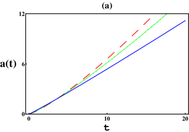
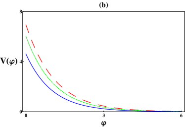
Figure 1: The plot of $a(t)$ and $V(\phi)$ for $n=-0.8$ and $s=0.08$ (dashed), $n=-0.85$ and $s=0.09$ (dotted) and $n=-0.95$ and $s=0.1$ (solid).

The figure shows that $V(\phi)$ has a run-away form as it should be since $\phi$ is a chameleon field [12].
The Universe has not been in an accelerating phase at all the time and has suffered a transition from an early decelerating phase to a recent accelerating one. To check that whether or nor the present model can generate such a phase transition, we look at the effective equation of state parameter $\omega_{eff}$. We first re-write (26) in the form

$$\dot{\rho_{b}}+3H(\omega_{eff}+1)\rho_{b}=0$$ (40)

where

$$\omega_{eff}=\omega_{b}+\frac{s}{3}+\frac{Q}{3H\rho_{b}}$$ (41)

$$~{}~{}~{}~{}~{}~{}~{}~{}~{}~{}~{}~{}~{}~{}~{}~{}~{}~{}~{}~{}~{}~{}~{}~{}~{}~{}~{}~{}\omega_{eff}=\frac{s}{3}-\frac{1}{3}\beta(\phi)\frac{\dot{\phi}}{H}~{}~{}~{}~{}~{}~{}~{}~{}~{}~{}~{}~{}~{}~{}~{}~{}~{}~{}~{}~{}(\omega_{b}=0)$$

Using the solution (38) and (39), gives $\frac{\dot{\phi}}{H}=2\sqrt{3}(\frac{-n}{(s+3)})^{\frac{1}{2}}$ which is a constant. This means that deceleration to acceleration phase transition needs $\beta(\phi)$ not to be a constant.
Among many possible choices for $\beta(\phi)$, let us choose a simple one $\beta(\phi)=\phi$ as an input coupling function. It corresponds to $A(\phi)=e^{\frac{1}{2}\phi^{2}}$. The resulting effective equation of state parameter is plotted in Fig.2.

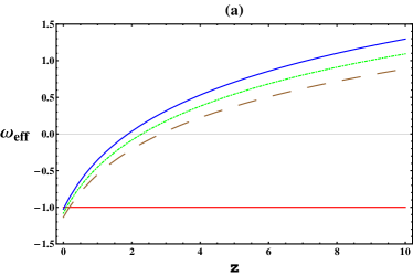
Figure 2: The plot of $\omega_{eff}$ in terms of $z$ for $\beta(\phi)=\phi$ panel (a) and $\beta(\phi)=\phi^{3}$ panel (b). The curves correspond to $n=-0.65$ and $s=0.08$ (dashed), $n=-0.7$ and $s=0.09$ (dotted) and $n=-0.75$ and $s=0.1$ (solid).

As it is clear from the figure, the function $\omega_{eff}$ exhibits a recent signature flip. It also shows that the Universe recently enters the phantom region.
The choice $\beta(\phi)=\phi$ is not the only one that leads to a transition from decelerating to accelerating phase. The panel (b) of the Fig.2 shows $\omega_{eff}$ for another choice $\beta(\phi)=\phi^{3}$. It should be remarked that in both cases deceleration to acceleration transition takes place when $\beta>0$ or $Q<0$. It means that in the interacting process described by (25) and (26), the direction of energy flow is so that matter is created. This seems to be consistent with the results reported in [17].

5 Thermodynamic Analysis

A thermodynamic description of a homogeneous and isotropic interacting perfect fluid requires a knowledge of the particle flux $N^{\alpha}=nu^{\alpha}$ and the entropy flux $S^{\alpha}=su^{\alpha}$ where $n=N/a^{3}$, $s=n\sigma$ and $\sigma=S/N$ is specific entropy (per particle) of the created or annihilated particles. Since energy density of matter is given by $\rho_{b}=nM$ with $M$ being the mass of each particle, the appearance of the extra term in the energy balance equation (26) means that this term can be attributed to a change of $n$ or $M$. Here we assume that the mass of each matter particle remains constant and the extra term in the energy balance equation only leads to a change of the number density $n$. In this case, the equation (26) can be written as

$$\dot{n}+3H(1+\frac{s}{3})n=n\Gamma$$ (42)

where $\Gamma\equiv\beta(\phi)\dot{\phi}$ is the rate of creation (or annihilation) of particles. The direction of energy transfer between matter and the scalar field depends on the sign of $\Gamma$. If $\Gamma>0$ (or $Q<0$), the energy goes inside of the matter system and matter is created. If $\Gamma<0$ (or $Q>0$) the direction of energy transfer is reversed and matter is annihilated.
From $\sigma=S/N$, we have

$$\frac{\dot{\sigma}}{\sigma}=\frac{\dot{S}}{S}-\frac{\dot{N}}{N}$$ (43)

With use of (42), the latter can be written as

$$\frac{\dot{S}}{S}=\frac{\dot{\sigma}}{\sigma}+(\Gamma-sH)$$ (44)

Since $n\propto a^{-3+(\epsilon-s)}$, the total number of particles scale as $N\propto a^{\epsilon-s}$. Thus (43) can also be written as

$$\frac{\dot{S}}{S}=\frac{\dot{\sigma}}{\sigma}+(\epsilon-s)H$$ (45)

In an adiabatic process, when the overall energy transfer is such that the specific entropy per particle remains constant ($\dot{\sigma}=0$) [18], the second law of thermodynamics ($\dot{S}\geq 0$) implies that $\epsilon-s\geq 0$ in an expanding Universe. In this case, when $\epsilon<0$ the parameter $s$ is allowed to take only negative values. Alternatively speaking, the extra dimension shrinks with expansion of the Universe (see (24)).
In the non-adiabatic case, on the other hand, the second law of thermodynamics requires that

$$\Gamma\geq sH-\frac{\dot{\sigma}}{\sigma}$$ (46)

which is also a constraint on the creation (or annihilation) rate and evolution of the extra dimension.

6 Conclusion

We have investigated a brane world scenario in which gravity is described by a five-dimensional metric together with a minimally coupled scalar field. The scalar field is a chameleon and interacts with the matter sector. Due to this interaction the energy associated with both the scalar field and matter system are not separately conserved. Thus evolution of matter energy density modifies and is controlled by $Q$. When $Q>0$ matter is created and energy is injecting into the matter system so that the latter will dilute more slowly compared to its standard evolution $\rho_{b}\propto a^{-3(\omega_{b}+1)}$. On the other hand, when $Q<0$ the reverse is true, namely that matter is annihilated and the direction of energy transfer is outside of the matter system (and into the scalar field) so that the rate of dilution is faster than the standard one.
The main results of our analysis are the following:
1) We have found a late-time asymptotic solution that exhibits accelerating expansion. There is also a recent transition from a decelerating phase to an accelerating one.
2) The interaction of chameleon field with matter plays an important role in this phase transition. In order that this transition takes place, the coupling function should be an evolving function (or $\beta(\phi)$ should not be a constant).
3) Our analysis also indicates that the Universe has recently entered the phantom region. We emphasize that this behavior is not attributed to any exotic matter system.
4) A thermodynamic analysis puts constraints on $\Gamma$ and evolution of the extra dimension in adiabatic and non-adiabatic cases.
There are some problems that are not investigated in the present analysis such as behavior of the Universe at early times or the cosmological constant problem. They are deserved to be investigated elsewhere.

References

- [1] L. Randall and R. R. Sundrum, Phys. Rev. Lett. 83 (1999) 3370 [arXiv:hep-ph/9905221].
- [2] L. Randall and R. Sundrum, Phys. Rev. Lett. 83 (1999) 4690 [arXiv:hep-th/9906064].
-
[3]
P. Brax and C. van de Bruck, Class. Quant. Grav. 20 (2003) R201
[arXiv:hep-th/0303095],
D. Langlois, Prog. Theor. Phys. Suppl. 148 (2003) 181 [arXiv:hep-th/0209261],
R. Maartens, Reference Frames and Gravitomagnetism, ed. J Pascual-Sanchez et. al., ( World Scientific, 2001 ), p.93-119 [arXiv:gr-qc/0101059]. -
[4]
P. Binetruy, C. Deffayet and D. Langlois, Nucl. Phys. B 565 (2000) 269
[arXiv:hep-th/9905012],
P. Binetruy, C. Deffayet, U. Ellwanger and D. Langlois Phys. Lett. B 477 (2000) 285 [arXiv:hep- th/9910219]. -
[5]
K. i. Maeda and D. Wands, Phys. Rev. D 62 (2000) 124009 [arXiv:hep-th/0008188],
S. C. Davis, JHEP 0203 (2002) 058 [arXiv:hep-ph/0111351],
M. Parry and S. Pichler, JCAP 0411 (2004) 005 [arXiv:hep-ph/0410025],
C. Bogdanos, A. Dimitriadis and K. Tamvakis, Class. Quant. Grav. 24 (2007) 3701 [arXiv:hep-th/0611181],
M. Heydari-Fard and H. R. Sepangi, JCAP 0901 (2009) 034 [ arXiv:gr-qc/0901.0855 ],
Arianto, F.P. Zen, S. Feranie, I P. Widyatmika, B.E. Gunara, Phys. Rev. D 84 (2011) 044008 [arXiv:gr-qc/1103.1703]. -
[6]
S. Kanno and J. Soda, Phys. Rev. D66 (2002) 083506 [arXiv:hep-th/0207029],
K. Yang, Y. Liu, Y. Zhong, X. Du and S.n Wei, Phys. Rev. D 86 (2012) 127502 [arXiv:hep-th/1212.2735]. -
[7]
K. Yang, Y. Liu, Y. Zhong, X. Du and S. Wei, Phys. Rev. D 86 (2012) 127502 [hep-th/1212.2735],
Q. Xie, Z. Zhao, Y. Zhong, J. Yang, X. Zhou, JCAP 1503 (2015) 014 [hep-th/1410.5911]. -
[8]
W.D. Goldberger and M.B. Wise, Phys. Rev. Lett. 83 (1999) 4922 [arXiv:hep-ph/9907447],
W.D. Goldberger and M.B. Wise, Phys. Rev. D60 (1999) 107505 [arXiv:hep-ph/9907218],
P. Kanti, K. A. Olive and M. Pospelov, Phys. Lett. B 481 (2000) 386 [arXiv:hep-ph/0002229]. - [9] Y. Himemoto and M. Sasaki, Phys. Rev. D 63 (2001) 044015 [arXiv:gr-qc/0010035].
- [10] J. Yokoyama and Y. Himemoto, Phys. Rev. D 64 (2001) 083511 [arXiv:hep-ph/0103115].
-
[11]
Kh. Saaidi and A. Mohammadi, Phys. Rev. D 85 (2012) 023526,
Kh. Saaidi, A. Mohammadi, T. Golanbari, H. Sheikhahmadi and B. Ratra, Phys. Rev. D 86 (2012) 045007. -
[12]
J. Khoury and A. Weltman, Phys. Rev. Lett. 93 (2004) 171104 [arXiv:astro-ph/0309300],
J. Khoury and A. Weltman, Phys. Rev. D 69 (2004) 044026 [arXiv:astro-ph/0309411]. -
[13]
J. Ponce de Leon, Gen. Rel. Grav. 38 (2006) 61-81 [arXiv:gr-qc/0412005],
J. Ponce de Leon, JCAP 1003 (2010) 030 [arXiv:1001.1961] - [14] N. Arkani-Hamed, S. Dimopoulos and G. Dvali, Phys. Lett. B 429 (1998) 263.
- [15] J.P. Uzan, Rev. Mod. Phys. 75 (2003) 403 [arXiv:hep-ph/0205340].
-
[16]
Y. Bisabr, Phys. Rev. D 86 (2012) 127503 [arXiv:1212.2709],
Y. Bisabr, Gen. Rel. Grav. 44 (2012) 427 [arXiv:1110.3421]. - [17] I. Prigogine, J. Geheniau, E. Gunzig, and P. Nardone, Gen. Rel. Grav. 21 (1989) 767.
- [18] J. A. S. Lima, Phys. Rev. D 54 (1996) 2571.