On the growth of eigenfunction averages: microlocalization and geometry
Abstract.
Let be a smooth, compact Riemannian manifold and an -normalized sequence of Laplace eigenfunctions, . Given a smooth submanifold of codimension , we find conditions on the pair for which
One such condition is that the set of conormal directions to that are recurrent has measure . In particular, we show that the upper bound holds for any if is surface with Anosov geodesic flow or a manifold of constant negative curvature. The results are obtained by characterizing the behavior of the defect measures of eigenfunctions with maximal averages.
1. Introduction
On a compact Riemannian manifold of dimension we consider sequences of Laplace eigenfunctions solving
In this article, we study the average oscillatory behavior of when restricted to a submanifold . In particular, we seek to understand conditions on the pair under which
| (1) |
as , where is the volume measure on induced by the Riemannian metric, and is the codimension of .
We note that the bound
| (2) |
holds for any pair [Zel92, Corollary 3.3], and is sharp in general. Therefore, we seek to give conditions under which the average is sub-maximal. Integrals of the form (1), where is a curve, have a long history of study. Good [Goo83] and Hejhal [Hej82] study the case in which is a periodic geodesic in a compact hyperbolic manifold, and prove the bound (2) in that case. The work of Zelditch [Zel92] in fact shows that (1) holds for a density one subsequence of eigenvalues. Moreover, one can give explicit polynomial improvements on the error term in (2) for a density one subsequence of eigenfunctions [JZ16].
These estimates, however, are not generally satisfied for the full sequence of eigenfunctions and the question of when all eigenfunctions satisfy (1) has been studied recently for the case of curves in surfaces [CS15, SXZ16, Wym17b, Wym17a] and for submanifolds [Wym17c]. Finally, given a hypersurface, the question of which eigenfunctions satisfy (1) was studied in [CGT17]. In this article, we address both of these questions, strengthening the results concerning which eigenfunctions can have maximal averages on a given submanifold , and giving weaker conditions on the submanifold that guarantee that (1) holds for all eigenfunctions.
This article improves and extends nearly all existing results regarding averages of eigenfunctions over submanifolds. We recover all conditions guaranteeing that the improved bound (1) holds found in [CS15, SXZ16, Wym17b, Wym17a, Wym17c, GT17, Gal17, CGT17, Bér77, SZ16a, SZ16b]. As far as the authors are aware, these papers contain all previously known conditions ensuring improved averages. Moreover, we give strictly weaker conditions guaranteeing (1) when ; we replace the condition that the set of loop directions has measure zero from [Wym17c] with the condition that the set of recurrent directions has measure zero. This allows us to prove that under conditions on including those studied in [Goo83, Hej82, CS15, SXZ16], the improved bound (1) holds unconditionally with respect to the submanifold . These improvements are possible because the main estimate, Theorem 6, gives explicit bounds on averages over submanifolds which depend only on the microlocalization of a sequence of eigenfunctions in the conormal directions to . This gives a new proof of (2) from [Zel92] with explicit control over the constant for high energies. In fact, we characterize those defect measures which may support maximal averages. The estimate requires no assumptions on the geometry of or and is purely local. It is only with this bound in place that we use dynamical arguments to draw conclusions about the pairs supporting eigenfunctions with maximal averages. We note, however, that this paper does not obtain logarithmically improved averages as in [Bér77, SXZ16, Wym17a].
Recall that all compact, negatively curved Riemannian surfaces have Anosov geodesic flow [Ano67]. One consequence of the results in this paper is the following.
Theorem 1.
Suppose is a compact, Riemannian surface with Anosov geodesic flow and is a smooth curve segment with . Then
as for every sequence of Laplace eigenfunctions. Here denotes the derivative in the normal direction to the curve.
In order to state our more general results we introduce some geometric notation. Let be a closed smooth submanifold of codimension . We denote by the conormal bundle to and we write for the unit conormal bundle of , where the metric is induced from that in . We write for the measure on induced by the Sasaki metric on (see e.g. [Ebe73a]). In particular, if are Fermi coordinates in a tubular neighborhood of , where is identified with , we have
where , , and is the dimensional sphere.
Let with
be the first return time. Define the loop set
and first return map by Next, consider the infinite loop sets
and the recurrent set
where
In what follows we write for the canonical projection map onto , and for the Minkowski box dimension of a set .
Theorem 2.
Let be a smooth, compact Riemannian manifold of dimension . Let be a closed embedded submanifold of codimension , and be a subset with boundary satisfying Suppose
Then
as for every sequence of Laplace eigenfunctions.
Theorem 2 improves on the work of Wyman [Wym17c], replacing the measure of the loop set , by that of the recurrent set . Taking to be a single point (i.e. ) also recovers the results of [STZ11]; see Remark 1.
When is a hypersurface, i.e. , we can also study the oscillatory behavior of the normal derivative along .
Theorem 3.
Suppose satisfy the assumptions of Theorem 2 with . Then for every sequence of Laplace eigenfunctions
as .
Theorem 2 allows us to derive substantial conclusions about the geometry of submanifolds supporting eigenfunctions with maximal averages. Indeed, if there exists and a sequence of eigenfunctions for which
then,
Next, we present different geometric conditions on which imply . We recall that strictly negative sectional curvature implies Anosov geodesic flow. Also, both Anosov geodesic flow and non-negative sectional curvature imply that has no conjugate points.
Theorem 4.
Let be a smooth, compact Riemannian manifold of dimension . Let be a closed embedded submanifold of codimension . Suppose one of the following assumptions holds:
-
A.
has no conjugate points and has codimension .
-
B.
has no conjugate points and is a geodesic sphere.
-
C.
has constant negative curvature.
-
D.
is a surface with Anosov geodesic flow.
-
E.
has Anosov geodesic flow and non-positive curvature, and is totally geodesic.
-
F.
has Anosov geodesic flow and is a subset that lifts to a horosphere.
Then
In addition, condition A implies that
Combining Theorems 2 and 4 gives the following result on the oscillatory behavior of eigenfunctions when restricted to .
Corollary 5.
We conjecture that the conclusions of Theorem 4, and hence also Corollary 5, hold in the case that is a manifold with Anosov geodesic flow of any dimension.
Conjecture.
Let be a manifold of dimension with Anosov geodesic flow and let be a submanifold of codimension . Then
1.1. Semiclassical operators and a quantitative estimate
This section contains the key analytic theorem for controlling submanifold averages (Theorem 6) which, in particular, has Theorems 2 and 3 as corollaries. We control the oscillatory behavior of quasimodes of semiclassical pseudodifferential operators using a quantitative estimate relating averages of quasimodes to the behavior of the associated defect measure. As a consequence, we characterize defect measures for which the corresponding quasimodes may have maximal averages.
We say that a sequence of functions is compactly microlocalized if there exists so that
Also, we say that is a quasimode for if
In addition, for , we say that a submanifold of codimension is conormally transverse for if given such that
we have
| (3) |
where is the Hamiltonian vector field associated to .
Let
and consider the Hamiltonian flow
We fix and define for a Borel measure on , the measure on by setting
Remark 2 in [CGT17] shows that if is a defect measure associated to a quasimode and is conormally transverse for , then is independent of the choice of . It is then natural to replace the fixed choice of with . In particular, for a defect measure associated to ,
| (4) |
for all Borel.
Next, let be the geodesic distance to . That is, . Then, define by
Finally, we write when and are mutually singular measures and let be the volume measure induced on by the Sasaki metric.
Theorem 6.
Let be a smooth, compact Riemannian manifold of dimension and have real valued principal symbol . Suppose that is a closed embedded submanifold of codimension conormally transverse for , and that is a compactly microlocalized quasimode for with defect measure . Let and be so that
Let and with . Then there exists , depending only on and , so that
| (5) |
In addition to relating the microlocalization of quasimodes to averages on submanifolds, Theorem 6 gives a quantitative version of the bound (2) proved in [Zel92, Corollary 3.3] and generalizes the work of the second author [Gal17, Theorem 2] to manifolds of any codimension. Note also that the estimate (5) is saturated for every on the round sphere .
Remark 1.
A direct consequence of Theorem 6 is the following.
Theorem 7.
Let be a smooth, compact Riemannian manifold of dimension . Let be a closed embedded submanifold of codimension , and let be a subset with boundary satisfying If is a sequence of eigenfunctions with defect measure so that , then
Theorem 7 strengthens the results of [CGT17]. In particular, in [CGT17], the measure is said to be conormally diffuse if , which of course implies
We note that Theorem 7 is an immediate consequence of Theorem 6. To see this, first observe that if we take , set , and let satisfy then
for any with on . Next, note that in this setting we have . Hence, if
then by Theorem 6,
To see that any is conormally transverse, observe that if , then . In particular, given there exists for which
1.2. Relation with bounds
Observe that taking in (2), and for some the estimate reads,
| (6) |
By Remark 1 the constant can be chosen independent of (and indeed, for small , depending only on the injectivity radius of and dimension of [Gal17]). Estimates of this form are well known, first appearing in [Ava56, Lev52, Hör68] (see also [Zwo12, Chapter 7]), and situations which produce sharp examples for (6) are extensively studied. Many works [Bér77, IS95, TZ02, SZ02, STZ11, SZ16a, SZ16b] have studied connections between growth of norms of eigenfunctions and the global geometry of the manifold . More recently [GT17, Gal17] examine the relation between defect measures and norms.
This article continues in the spirit of [GT17, Gal17] and, in particular, taking in Theorem 6 (together with Remark 1) recovers [Gal17, Theorem 2]. Hence this article also generalizes many of the results of [SZ02, STZ11, SZ16a, SZ16b] to manifolds of lower codimension. For example taking in Theorem 2 gives the main results of [STZ11] (see also [Gal17, Corollary 1.2]).
1.3. Manifolds with no focal points or Anosov geodesic flow
In order to prove parts C, D, E and F of Theorem 4, we need to use that the underlying manifold has no focal points or Anosov geodesic flow. We show that these structures allow us to restrict to working on the set of points in at which the tangent space to splits into a sum of bounded and unbounded directions. To make this sentence precise we introduce some notation.
If has no conjugate points, then for any , there exist stable and unstable subspaces so that
and
Moreover, if has no focal points then vary continuously with . (See for example [Ebe73a, Proposition 2.13].)
In what follows we write
We define the mixed and split subsets of respectively by
Then we write
| (7) |
where we will use when considering manifolds with Anosov geodesic flow and when considering those with no focal points.
Next, we recall that any manifold with no focal points in which every geodesic encounters a point of negative curvature has Anosov geodesic flow [Ebe73a, Corollary 3.4]. In particular, the class of manifolds with Anosov geodesic flows includes those with negative curvature. We also recall that a manifold with Anosov geodesic flow does not have conjugate points and for all
where are the stable and unstable directions as before. (For other characterizations of manifolds with Anosov geodesic flow, see [Ebe73a, Theorem 3.2], [Ebe73b].) Moreover, there exists so that for all ,
and the spaces are Hölder continuous in [Ano67].
Theorem 8.
Let be a closed embedded submanifold.
If has no focal points, then
If has Anosov geodesic flow, then
Corollary 9.
Let be a closed embedded submanifold of codimension , and let satisfy . Then if has no focal points and
we have
| (8) |
as for every sequence of Laplace eigenfunctions. If instead has Ansov geodesic flow then (8) holds when
Note that if , then since . Indeed, it is not possible to have both and unless and hence . In [Wym17b, Wym17a] the author works with non-positively curved (and hence having no focal points), and a curve. He then imposes the condition that for all time the curvature of , , avoids two special values determined by the tangent vector to , . He shows that under this condition
If , then the lift of to the universal cover of is tangent to a stable or unstable horosphere at and is equal to the curvature of that horosphere. Since this implies that is stable or unstable, the condition there is that Thus, the condition is the generalization to higher codimensions of that in [Wym17b, Wym17a]. We note that [Wym17a] obtains the improved upper bound .
1.4. Organization of the paper
We divide the paper into two major parts. The first part of the paper contains all of the analysis of solutions to . The sections in this part, Section 2 and Section 3, contain the proofs of Theorem 6 and Theorem 3 respectively. The second part of our paper, consists of an analysis of the geodesic flow and in particular a study of the recurrent set of . Theorem 2 is proved in Section 4, and Theorems 4 and 8 are proved in Section 5.
Note that as already explained, Corollary 5 is an immediate consequence of combining Theorems 2 and 4.
Also, Theorem 7 is a direct consequence of Theorem 6 and Corollary 9 is a consequence of Theorem 2 and Theorem 8.
Finally, Theorem 1 is exactly part D of Theorem 4.
Acknowledgements. Thanks to Semyon Dyatlov, Patrick Eberlein, Colin Guillarmou, and Gabriel Paternain for several discussions on hyperbolic dynamics. J.G. is grateful to the National Science Foundation for support under the Mathematical Sciences Postdoctoral Research Fellowship DMS-1502661.
2. Quantitative estimate: Proof of Theorem 6
In Section 2.1 we present the ground work needed for the proof of Theorem 6. In particular, we state the main technical result, Proposition 10, on which the proof of Theorem 6 hinges. We then divide the proof of Theorem 6 in two parts. Assuming the main technical proposition, we first prove the theorem for the case and in Section 2.2, and then generalize it to any subset in Section 2.3. Finally, Section 2.4 is dedicated to the proof of Proposition 10.
Throughout this section we assume that has principal symbol and is conormally transverse for as defined in (3). We also assume throughout this section that is a compactly microlocalized quasimode for .
2.1. Preliminaries.
Let be a smooth closed submanifold and let be an open neighborhood of described in local coordinates as where these coordinates are chosen so that . The coordinates induce coordinates on with , and where we continue to write . In these coordinates, is cotangent to while is conormal to . Since is conormally transverse for , we may assume, without loss of generality, that with dual coordinates where
Consider the cut-off function with
| (9) |
with for all . For consider the symbol
| (10) |
where is the Riemannian metric on induced by . Let , where denotes the interior of . We start splitting the period integral as
The same proof as [CGT17, Lemma 8] yields that for all
(see also Lemma 12).
Choosing , and using the restriction bound from [BGT07], we obtain that
| (11) |
We control the integral of using the following lemma. Recall that we write for the Hamiltonian vector field corresponding to and for the associated Hamiltonian flow. To shorten notation, we write
Proposition 10.
Let so that on for some . Let . There exists depending only on and so that
The proof of Proposition 10 is given in Section 2.4. The purpose of this proposition is to allow us to use to localize quasimodes to the support of and its complement. Since and are mutually singular, it is not difficult to see that Proposition 10 gives a bound for of the form . By further restricting to shrinking balls inside an application of the Lebesgue differentiation theorem allows us to obtain a bound of the form as claimed. This improvement will be needed when passing to subsets . The factor measures the cost of restricting to a hypersurface containing which is microlocally transversal to . In particular, we choose coordinates so that and at a point . This is possible since is conormally transverse for .
To apply Proposition 10 it is key to work with cut-off functions so that on for some . Therefore, the following lemma is dedicated to extending cut-off functions on to cut-off functions on that are invariant under the Hamiltonian flow inside . Let be so that
is a diffeomorphism for all . Such a exists since is compact and conormally transverse for . Moreover, for , is a closed embedded submanifold in .
Lemma 11.
For all and there exists
so that
for all and . In particular, on .
Proof.
Let be a fixed function supported on with on . Then, using that is a diffeomorphism, define the smooth cut-off by the relation
Finally, extend to all of so that . We can make such an extension since is a closed embedded submanifold in . ∎
2.2. Proof of Theorem 6 for
Fix . Since and are two Radon measures on that are mutually singular, there exist compact and with and so that
Indeed, by definition of mutual singularity, there exist so that and . Hence, by outer regularity of , there exists open with Next, by inner regularity, of , there exists compact with Let be a cut-off function with
Let be the cut-off extension of given in Lemma 11 with
where we have fixed so that . We use (11) and split the period integral as
Applying Proposition 10 with , we have that
| (12) | ||||
Here we have used that and that by construction .
We dedicate the rest of the proof to showing that
We start by splitting the left hand side in (13) into an integral over small balls. By the Besicovitch–Federer Covering Lemma [Hei01, Theorem 1.14, Example (c)], there exists a constant depending only on and so that for all , there exist open balls of radius with
so that
and each point in lies in at most balls. Let with be a partition of unity associated to , and write for the extensions given in Lemma 11 so that for all and . With this construction, on ,
Let . Setting we have on and (since on ). We then apply Lemma 10 to , to obtain
On the other hand, by the triangle inequality we have
By construction we have that on . We may therefore apply Proposition 10 with to find that there exist so that
Here we have used that and for small enough for all , and some depending only on . It follows that there is for which
Decomposing , and using that
while , we conclude that there exists so that
| (14) |
where
Since for small enough, and any , we have , there exists so that
The Lebesgue Differentiation Theorem [Fol99, Theorem 3.21] shows that
Furthermore, the weak type 1-1 boundedness of the Hardy–Littlewood maximal function [Fol99, Theorem 3.17] implies that there exists so that for every
2.3. Proof of Theorem 6 for any
In order to pass to , we break the integral into two pieces. First, near the conormal bundle , we approximate by an (-independent) smooth function and apply the theorem on all of . In order to estimate the piece away from , we approximate by a smooth function depending badly on . We are then able to perform integration by parts to estimate contributions away from and a simple volume bound near .
Let be a subset with and indicator function Extend to another closed, embedded submanifold of codimension so that is compactly contained in the interior . We will actually apply Theorem 6 to and . Since is dense in , for any , we can find a positive function with
For any and ,
We claim that if has boundary satisfying Then, for all and ,
| (16) |
We postpone the proof of (16) until the end. Assuming that (16) holds, the universal upper bound [BGT07] together with Cauchy-Schwarz give
| (17) |
Next, note that and apply Cauchy–Schwarz to obtain
for some . Finally, to bound the second term in (17) we note that
and that by Theorem 6 with and there exists for which
The last equality follows from Cauchy-Schwarz and the bound . This gives the stated result provided (16) holds. We proceed to prove (16).
To prove (16) we first introduce a cut-off function so that is smooth and close to and is in a neighborhood of . For this, fix and cover by -dimensional cubes , with , and side length with disjoint interiors. This can by done so that
We decompose
| (18) |
We bound using that is -bounded and that has compact support. We proceed to bound . Cover each cube by open balls of radius . Let be a partition of unity near subordinate to and define . Then,
| (19) |
Moreover, since the volume of each cube is , there is so that
It follows that
| (20) |
On the other hand, the function satisfies the bounds (19). In particular, putting in Lemma 12 below, for ,
| (21) |
∎
Lemma 12.
Suppose that satisfies (19) for some . Then, for ,
Proof.
2.4. Localizing near bicharacteristics: Proof of Proposition 10
Throughout the proof of Proposition 10 we will need the following lemma. Since it is a local result, we state it for functions and operators acting on . We write for coordinates in and for the dual coordinates.
Lemma 13.
Let be a smooth function with compact support and fix with
Then, there exists and a neighborhood of so that for all the following holds. Let be a neighborhood of and with
Let , with in a neighborhood of , and . Then, there exists so that the following hold.
If , then
If , then
The proof of Lemma 13 is very similar to that of [Gal17, Lemma 4.3], although some alterations are needed. For the sake of completeness we include the proof at the end of this section, in 2.4.4.
2.4.1. Case: is hypersurface.
We proceed to explain the role that Lemma 13 has in the proof of Proposition 10. To do this, we assume for a moment that is a hypersurface (, and use local coordinates near it with . This section is a particular case of the results presented in Section 2.4.2 where with any codimension is treated.
Let , and let with
Define
Also, let supported sufficiently close to satisfy
where and is defined in (26).
We choose Fermi coordinates with respect to so that
Moreover, in these coordinates . Hence, we will apply Lemma 13 with and (here we shrink the support of if necessary). In order to apply the lemma, we note that
and define so that
| (22) |
Next, let be an extension of off of so that in a neighborhood of . Applying Lemma 13 with , , , and , gives the existence of independent of so that
Next, we use that , , and
| (23) |
In addition, by (22) and the fact that , we have
Therefore,
| (24) | ||||
| (25) |
2.4.2. Case: has any codimension .
In the case in which has any codimension , the proof of Proposition 10 hinges on Lemma 14 below. This lemma is dedicated to obtaining a gain in the bound for by localizing in phase space near bicharacteristics emanating from . The key idea is that microlocalization near a family of bicharacteristics parametrized by implies a quantitative gain in the norm. By decomposing into many pieces microlocalized along well-chosen families of bicharacteristics, we are able to extract Proposition 10.
Let be a smooth section (i.e. and ); where we continue to write .
Let supported near . We choose Fermi coordinates with respect to , , so that and, making additional rotation in if necessary, so that
Moreover, note that for supported near we have .
For each in the projection of onto define a function so that vanishes on the bicharacteristic emanating from . This is possible since we have chosen coordinates so that
and hence the bicharacteristic emanating from may be written locally as
| (26) |
where is small enough, and are smooth functions depending on . Indeed, if we write , we have that which allows us to use the inverse function theorem to locally write as a function of .
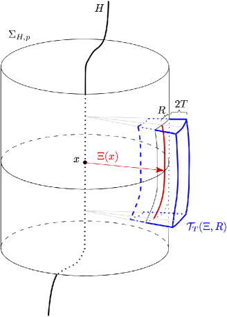
To exploit the construction of the function we further localize in phase space on tubes of small radius that cover . We define the tubes
| (27) |
where describes the distance in between the points and (see Figure 1 for a schematic picture of these objects).
The spirit of the following result is similar to that of [Gal17, Lemma 5.2]. Lemma 14 is dedicated to showing that microlocalizing with supported on gives an gain in the bound for . This is a generalization of the relation (25) already discussed in the case in which is a hypersurface.
Lemma 14.
Let supported sufficiently close to satisfy
where and is defined in (26). Let be a smooth section. There exists depending only on so that for all and if
| (28) |
then there exists depending only on and so that
| (29) |
where is any extension of for which on . In addition, if the assumption in (28) is not enforced, then (29) holds with .
Proof.
In what follows we write for the normal coordinates to that are not . With this notation . As before, let with
Define also
and with
Using that , we bound
for
where and is defined in (26). The reason for working with this function is that
for , and this will allow to obtain a gain in the -norm bound, since, as we will see below, . We bound using the version of the Sobolev Embedding Theorem given in [Gal17, Lemma 5.1] which states that if , then for all there exists depending only on and so that
for all , . Now, for all , integrate in to get
In particular, setting on the left hand side we get
| (30) |
We will end up choosing and .
Remark 2.
Note that when (i.e. in the case of is a hypersurface), estimates on the derivatives are not necessary.
By (3) we may assume, without loss of generality, that on . Hence, we will apply Lemma 13 with and (here we shrink the support of if necessary). In order to apply the lemma we define as in (22), where we change for . Next, let be an extension of off of so that in a neighborhood of . We do this as in Lemma 11 using that is transverse to to solve the initial value problem.
We now choose to obtain a gain in the restriction norm related to . Let
Applying Lemma 13 with , , , and , we have
with independent of . Here we have used that in our coordinates
Applying (30) gives that for any
| (31) |
In particular, since is the defect measure associated to , arguing as in (23) we obtain
Next, we observe that by (22) and the fact that , we have
Sending and using on (together with to apply the Dominated Convergence Theorem) we have
| (32) | ||||
Remark 3.
We now present the proof of Proposition 10.
2.4.3. Proof of Proposition 10.
Let so that on for some . Also, fix .
For all , we can find and with so that if we set
where and are balls of radius and respectively, then
and
Let be a partition of unity for subordinate to . Apply Lemma 11 to obtain the flow invariant extensions
so that
-
(1)
,
-
(2)
,
-
(3)
,
-
(4)
on ,
-
(5)
.
We then have
Now, to recover the spatial localization we introduce with and
Then,
In fact, on with the standard quantization, we have . Hence, the above estimate follows from the fact that quantizations differ by together with the standard restriction estimate for compactly microlocalized functions.
In what follows we bound using Lemma 14 applied to . This can be done since on . Lemma 14 yields that there exists depending only on and so that, for any extension of with on , and ,
We have used that there exists so that for and small enough
that by continuity of on , as ,
and the dominated convergence theorem.
Since is arbitrary, this completes the proof of the proposition.
∎
2.4.4. Proof of Lemma 13.
First, suppose is so that . Then, there exists a neighborhood of with . One can then carry an elliptic parametrix construction so that
| (34) |
for all supported in and some suitable . Therefore,
as claimed. We may assume from now on that
By the implicit function theorem, for supported sufficiently close to , and
with elliptic on and . In particular,
Therefore,
where we have set
and denotes a microlocal parametrix for near . Defining
we obtain that for all
Let be so that
| (35) |
and with and . Then, integrating in ,
Next, applying propagation of singularities, we claim that
| (36) | ||||
with . Indeed, (36) follows once we show that for any supported on and
| (37) |
Let be as in (9). By the same construction carried in (34) (which gives that is microlocalized on ) we conclude
| (38) |
Therefore, to prove (37) we need to estimate
Let denote the Hamiltonian flow of . Then, for and , we have . By (22), is identically 1 in a neighborhood of
and thus for small enough on
In particular, since we assume that and satisfies (35), we have
| (39) |
Together (38) and (39) give (37). In particular, we obtain (36) which, since
implies
Now,
Therefore, since
we have the following bound along the section
| (40) |
finishing the proof.
∎
3. Proof of Theorem 3
When the codimension of is equal to and is compact we can include an estimate on the normal derivate in all of our results. In particular, for a unit normal to , we may replace all instances of with
To see this, observe that if is a quasimode for and is compactly microlocalized, then
In particular,
| (41) |
Let have in a neighborhood of and
Then, there exists so that
and in particular, applying to (41) we find
Now, . Therefore, since in a neighborhood of and is conormally transverse for , is conormally transverse for . Thus, Theorem 6 applies and gives
where
with and is the defect measure for . It is straightforward to see that
and hence (for chosen small enough)
In particular,
since is compact and is supported on .
Remark 4.
Note that the constant now depends on .
4. Proof of Theorem 2
We prove Theorem 2 by contradiction. Suppose that there exists a sequence and such that
| (42) |
Then, we may extract a subsequence (still writing it as ) with defect measure . Let be the induced measure on and be the measure on with and so that
for . Then,
| (43) |
where the last equality follows from the fact that . Also, since , there exist so that and . Next, we use that Lemma 15 below gives . It follows that
| (44) |
Combining (43) and (44) gives , and so Theorem 7 gives a contradiction to (42).
∎
Lemma 15.
Let and suppose that is a sequence of eigenfunctions with defect measure . Then,
Proof.
Let be an open set and for define
Observe that the triple forms a measure preserving dynamical system. The Poincaré Recurrence Theorem [BS02, Lemma 4.2.1, 4.2.2] implies that for -a.e. there exist so that . By the definition of , there exists with such that . In particular, for -a.e. ,
| (45) |
We have used that the sets are non-empty, compact, and nested as grows.
We next show that (45) holds for -a.e. point in . To do so, suppose the opposite. Then, there exists with so that for each , there exists with
| (46) |
We relate and using [CGT17, Lemma 6] which gives
Then, if we let
we have
Then , and for all there exists so that (46) holds. Since this implies that (45) does not hold for a subset of of positive measure, we have arrived at a contradiction. Thus (45) holds for a.e. point in .
To finish the argument, let be a countable basis for the topology on . Then for each there is a subset of full measure so that for every relation (45) holds with .
Let . Next, note that . Indeed, if and is an open neighborhood of , then there exists so that . In particular, since , we know that and so We conclude that returns infinitely oftern to .
Noting that has full measure, we conclude that has full measure and thus as claimed. ∎
5. Recurrence: Proof of Theorem 4
This section is dedicated to the proof of Theorem 4. In Section 5.1 we prove the theorem for assumptions A and B by showing that . In Section 5.2 we present a tool for proving that for . In particular, we prove that it suffices to show that is integrable either for positive times or for negative ones. In Section 5.3 we show that for manifolds with Anosov flow we have , where is the set of points in at which the tangent space to splits into a direct sum of stable and unbounded directions. A similar statement is proved for with no focal points, but with instead of . In Section 5.4 we prove Theorem 4 for assumptions C, D, E and F, by taking advantage of the fact when has Anosov flow we have some control on the structure of and, in some cases, on the integrability of .
5.1. Proof of parts A and B
In this section we prove that for and satisfying the assumptions in parts A and B in Theorem 4.
Proof of part A. For this part we assume that has no conjugate points and has codimension .
The strategy of the proof is to show that the set has dimension strictly smaller than , and hence has measure zero. We prove this using the implicit function theorem together with the fact that, since has no conjugate points, we can control the rank of the exponential map.
Note that, since has no conjugate points, for each point the exponential map has no critical points. In particular, if we define the map
we have for all
This implies that if we define
then its differential
has
for all . Note that .
Let
| (47) |
The composition satisfies . Note that since , we have
for . Since by assumption , we have
Moreover, since the geodesic flow is transverse to along , whenever . Indeed, suppose that and . Then, if we write , we have that for all , and this contradicts the assumption that are linearly independent and span for .
Applying the Implicit Function Theorem, we see that given with , there exists a neighborhood of , an open neighborhood of for some , and smooth functions , with , , so that
In particular, since ,
In particular, by compactness, for any ,
Taking the union over we find
In particular, since , this implies that . ∎
Proof of part B.
Now, suppose that has no conjugate points and is a geodesic sphere. Then there exists and so that for .
Applying the result in Part A gives that . In particular, by Lemma 16 below we conclude
as claimed.
∎
Lemma 16.
Suppose that is a submanifold and for define . Then, for any so that is a smooth submanifold of having codimension
| if and only if |
Proof.
First, observe that if is a submanifold, then for and , we have
whenever is a smooth submanifold of . To see this, observe that since has codimension 1, for each , there are exactly two elements in and hence these elements are given by
for some . Note that . Therefore, since is a diffeomorphism onto its image, if and only if . ∎
5.2. A tool for proving that .
Given submanifold, we write for the volume induced by the Sasaki metric on . This section is dedicated to showing that whenever the map is integrable either on or on . We will later use that the integrability of this function can always be established if has Anosov flow and is a set of points in at which the tangent space is either stable or unstable.
We start with a lemma where we prove that for any the tangent space has no component in the direction of .
Proposition 17.
Let be a Riemannian manifold, and let be a submanifold. For all let be the orthogonal projection map, where is the Hamiltonian flow associated to . Then,
Proof.
Let be Fermi coordinates near where we identify with . Writing for the associated cotangent coordinates,
This implies that, if , then
while
Now, is orthogonal to . Thus, since is vertical and is horizontal is orthogonal to . ∎
Lemma 18.
Let .
| (48) | |||
| (49) |
In particular, either assumption implies that .
Proof.
We claim that there exist constants so that for any Borel set and ,
| (51) |
Note that since is a smooth group, for small enough and ,
| (52) |
Hence,
In order to finish the proof of the lemma we need to establish the claim in (51). We proceed to do this. Fix . Let be a partition of into sets of radius less than . Then for each , there exists so that for ,
where is the projection operator and is regarded as a vector in . Therefore,
Now, Proposition 17 together with the compactness of give that for small enough and all ,
Sending , since is continuous, the Dominated Convergence Theorem shows that
| (53) |
as desired. ∎
5.3. Manifolds with no focal points or Anosov flow
This section is dedicated to the proof of Theorem 8. In order to prove Theorem 8 we need a preliminary lemma in which we show, loosely speaking, that if is a loop direction for which , then it suffices to find a tangent direction with the property that is not tangent to to ensure that for almost every so that is near .
Lemma 19.
Suppose that with for some . If there exists with , then there exists a neighborhood of for which
Proof.
We use the Implicit Function Theorem. Define
so that
and let be defining functions for near . In particular,
Finally, let be given by
Note that if and only if . Now, since , Proposition 17 gives that the vectors
and
are linearly independent. We then have that
By the implicit function theorem, there is a neighborhood of , a neighborhood of for some , and smooth functions , with , , so that
In particular, since ,
as claimed. ∎
Next we present two propositions in which we show that if has no focal points or Anosov geodesic flow, then for any compact subset there is a decomposition of , and sufficiently large so that if and with either , then there exists with . This will allow us to later use Lemma 19 to prove Theorem 8. We define the following functions
| (54) |
and note that the continuity of implies that are upper semicontinuous.
Proposition 20.
Suppose has Anosov geodesic flow and let be a compact set. There exist positive constants so that if , , and
then there is with
| (55) |
Proof.
Let . Since , we may choose
Now, let and be so that
Without loss of generality, we assume that is orthogonal to and, since varies in a compact subset of , we may assume uniformly for that
Since is an isomorphism,
Note that for as in (54), is upper semicontinuous and we may choose uniform in , so that for all such that For such values of we then have
| (56) |
Next, we note that . Also, note that if , then . In particular, relation (56) gives that there exists a linear combination
with , so that
where is the orthogonal projection map onto a subspace of chosen so that is an orthogonal decomposition. If we had that was a tangent vector in , then we would be done. However, since is not necessarily in we have to modify a bit. Consider the vector
and note that . Then,
By the definition of Anosov geodesic flow, for all , there exists so that
Thus, since and , we have
Observe next, [Ebe73a, Corollary 2.14] that there exists uniform in so that for , and In particular, choosing , for ,
Hence, there exists and (uniform for ) so that if for some with , then there is so that
| (57) |
∎
We next introduce the following result in which we show that for manifolds with Anosov geodesic flow the set of points in has measure zero.
Lemma 21.
Suppose that has Anosov geodesic flow. Then
and
In particular,
Proof.
In what follows we write
and note that
Note that
Proposition 22.
Suppose has no focal points and let be a compact set. There exist positive constants so that if , , and
then there is with
| (58) |
Proof.
We prove the lemma for , the other case follows similarly after sending rather than .
Define as the conic set of vectors forming at least an angle with . Since is upper semicontinuous, is continuous, and , there exists so that for all .
Next, let . Since , the upper semicontinuity of implies that for all , after possibly shrinking . In particular, the continuity of implies that there exists so that for , the angle between and is larger than (after possibly shrinking ).
To finish the argument we argue by contradiction. Suppose that for , we have and
Then, using that , we conclude from the claim in (59) applied to some that there exists so that the angle between and is smaller than . In particular, setting we conclude that the angle between and is smaller than . And this is a contradiction since . This concludes the proof of the proposition once we have (59).
It only remains to prove the claim in (59). Let . Then we can write
with and , where denotes the collection of vertical vectors in orthogonal to . Note that there exists depending only on so that
For any we decompose
| (60) |
and find so that each term in the RHS has size smaller than .
Note that since is vertical, the Jacobi field through with initial conditions given by and , where and denote respectively the horizontal and vertical parts, has and hence, by [Ebe73a, Remark 2.10], there exists so that for in a compact set,
In particular, for all , there exists so that
| (61) |
Next, observe that by [Ebe73a, Remark 2.10], for all , there exists so that for all , and ,
| (62) |
In particular, by (62), given there exists so that for and ,
Furthermore, by [Ebe73a, Corollary 2.14], there exists so that for all and all ,
| (63) |
In particular, setting , and letting ,
| (64) |
On the other hand, for ,
| (65) |
Taking we conclude that the claim in (59) holds after combining (61),(64), and (65), into (60).
∎
Now that we have introduced Propositions 17, 22, and 20, we are ready to present the proof of Theorem 8.
Proof of Theorem 8. We start with the case in which has no focal points. Recall, that from (54) are upper semicontinuous. In particular, the sets
are open, and hence are open as well. Thus, there exist collections of compact sets
with
Since
the proof of the lemma will follow once we prove that for any compact subset
| (66) |
We then proceed to prove (66).
Let and be the constants associated to given by Proposition 22. Since
with
we have that (66) is a consequence of showing that
| (67) |
for all with .
To prove (67) let . Since for some , and , Proposition 22 combined with Lemma 19 give that there exists a neighborhood of for which
Since, is compact if is closed, is compact and we can cover by finitely many such neighborhoods and in particular,
and hence . Therefore, we have (67) provided we show that is closed
We dedicate the end of the proof to showing that is closed. To see this, let with . For each let be so that . By possibly taking a subsequence of times, we may assume that there exists with the property that as . In particular, we have that . Then, the triangle inequality
shows that as claimed.
5.4. Proof of parts C, D, E and F
Since in all these cases has Anosov flow, for all ,
where are stable and unstable directions as before. Moreover, there exists so that for all ,
Proof of part E.
For this part we assume that has Anosov geodesic flow, non-positive curvature, and is totally geodesic.
We use that, since there are no parallel Jacobi fields on a manifold with non-positive curvature and Anosov geodesic flow [Ebe73b, Theorem 1 (6)], the spaces and are nowhere horizontal. In particular, for any horizontal vector , for . To take advantage of this, fix . Since is totally geodesic, the horizontal lift of any satisfies
On the other hand,
Suppose that is dimensional. Then, we may choose linearly independent vectors and get
In particular, this yields that
Therefore,
and hence .
To finish the proof we explain that it suffices to assume that is dimensional. Note that since is totally geodesic submanifold, is also a totally geodesic submanifold. Now, for small,
is an isometry, and in particular, is an embedded submanifold of dimension . Moreover, by Lemma 16, implies Therefore, it is enough to show that for every totally geodesic submanifold of dimension which we have already done.
∎
The proofs of Parts C, D, and F, rely on showing that in each of these settings one has that the set of points for which is purely stable, or purely unstable, has full measure and applying Lemma 21.
Proof of part D.
For this part we assume that is a surface with Anosov geodesic flow. Theorem 8 implies
But, since , we have and, since , . Thus, as claimed. ∎
Proof of part F.
For this part we assume that has Anosov geodesic flow and is a subset of a stable or unstable horosphere. That follows immediately from Lemma 21. ∎
Proof of part C. We start by showing that it suffices to assume that is dimensional. Since the exponential map is a radial isometry, is an embedded submanifold of dimension for small . Moreover, by Lemma 16, implies Therefore, it is enough to show that for every submanifold of dimension .
We note that by Theorem 8 we have
Lemma 23.
Let be a compact manifold with constant negative curvature and be a closed embedded hypersurface. Then
The rest of this section is dedicated to the proof of Lemma 23. Since we may work locally to prove Lemma 23, we lift the hypersurface to the universal cover . Hence, in this section we work with the hyperbolic space
We endow with the metric . To prove Lemma 23 we adopt the notation
for the inner product induced by the metric . We also write for the usual inner product in . With this notation the sphere bundle takes the form , and its tangent space at can be decomposed into a direct sum where the stable and stable fibers are and and is the generator of the geodesic flow. Since we work in the co-sphere bundle, we record the structure of the dual spaces. The co-sphere bundle is
and the tangent space at any is
We then have
where
| (68) |
and
| (69) |
Here, and in what follows, we adopt the notation to represent a point in .
Proof of Lemma 23..
We assume that is a parametrization of in a neighborhood of . That is,
for some open, and where
Using that and are defining functions for as a subset of we find that
where to shorten notation we write
This yields that
where
Therefore, given we find
| (70) |
where
We assume without loss of generality that , where and . Note that, with
where is an symmetric matrix we have
Now, suppose there exist two non-zero vectors
Then, according to (70), (68) and (69) we have that there exist so that
and satisfying
-
i)
-
ii)
-
iii)
-
iv)
-
v)
.
We proceed to showing that there cannot exist satisfying conditions and for all in a subset of with positive measure on which , and . Indeed, conditions and read
-
i)
-
ii)
-
iii)
These equations imply that and so . Furthermore, we claim that we may assume that . Indeed, let be so that . Then, if , we may decompose it as and use that condition gives . If we had that condition holds on a set of ’s with positive measure, we must have that since we just showed that condition should also hold for all . We then work with
From this we get the improved estimates
We derive the contradiction from studying the second order terms in . Indeed,
where
and where denotes the vector whose -th entry is given by . Since is a second order term in , equation gives that
To take advantage of this condition, we assume without loss of generality that
where is an matrix, and that
We now use that all the coordinates of the vectors equal . Making the second coordinate of the vector equal to gives
while setting the first coordinate of the vector equal to yields
This concludes the proof since we cannot have the two relations holding simultaneously for in a subset of that has positive measure.
∎
References
- [Ano67] D. V. Anosov, Geodesic flows on closed Riemannian manifolds of negative curvature, Trudy Mat. Inst. Steklov. 90 (1967), 209. MR 0224110
- [Ava56] Vojislav G. Avakumović, Über die Eigenfunktionen auf geschlossenen Riemannschen Mannigfaltigkeiten, Math. Z. 65 (1956), 327–344. MR 0080862
- [Bér77] Pierre H. Bérard, On the wave equation on a compact Riemannian manifold without conjugate points, Math. Z. 155 (1977), no. 3, 249–276. MR 0455055
- [BGT07] N. Burq, P. Gérard, and N. Tzvetkov, Restrictions of the Laplace-Beltrami eigenfunctions to submanifolds, Duke Math. J. 138 (2007), no. 3, 445–486. MR 2322684
- [BS02] Michael Brin and Garrett Stuck, Introduction to dynamical systems, Cambridge University Press, Cambridge, 2002. MR 1963683
- [CGT17] Yaiza Canzani, Jeffrey Galkowski, and John A. Toth, Averages of eigenfunctions over hypersurfaces, arXiv preprint arXiv:1705.09595 (2017).
- [CS15] Xuehua Chen and Christopher D. Sogge, On integrals of eigenfunctions over geodesics, Proc. Amer. Math. Soc. 143 (2015), no. 1, 151–161. MR 3272740
- [Ebe73a] Patrick Eberlein, When is a geodesic flow of Anosov type? I, Journal of Differential Geometry 8 (1973), 437–463.
- [Ebe73b] by same author, When is a geodesic flow of Anosov type? II, J. Differential Geometry 8 (1973), 565–577.
- [Fol99] Gerald B. Folland, Real analysis, second ed., Pure and Applied Mathematics (New York), John Wiley & Sons, Inc., New York, 1999, Modern techniques and their applications, A Wiley-Interscience Publication. MR 1681462
- [Gal17] Jeffrey Galkowski, Defect measures of eigenfunctions with maximal growth, arXiv preprint arXiv:1704.01452 (2017).
- [Goo83] Anton Good, Local analysis of Selberg’s trace formula, Lecture Notes in Mathematics, vol. 1040, Springer-Verlag, Berlin, 1983. MR 727476
- [GT17] Jeffrey Galkowski and John A Toth, Eigenfunction scarring and improvements in bounds, arXiv preprint arXiv:1703.10248 (2017).
- [Hei01] Juha Heinonen, Lectures on analysis on metric spaces, Universitext, Springer-Verlag, New York, 2001. MR 1800917
- [Hej82] Dennis A. Hejhal, Sur certaines séries de Dirichlet associées aux géodésiques fermées d’une surface de Riemann compacte, C. R. Acad. Sci. Paris Sér. I Math. 294 (1982), no. 8, 273–276. MR 656806
- [Hör68] Lars Hörmander, The spectral function of an elliptic operator, Acta Math. 121 (1968), 193–218. MR 0609014
- [IS95] H. Iwaniec and P. Sarnak, norms of eigenfunctions of arithmetic surfaces, Ann. of Math. (2) 141 (1995), no. 2, 301–320. MR 1324136
- [JZ16] Junehyuk Jung and Steve Zelditch, Number of nodal domains and singular points of eigenfunctions of negatively curved surfaces with an isometric involution, J. Differential Geom. 102 (2016), no. 1, 37–66. MR 3447086
- [Lev52] B. M. Levitan, On the asymptotic behavior of the spectral function of a self-adjoint differential equation of the second order, Izvestiya Akad. Nauk SSSR. Ser. Mat. 16 (1952), 325–352. MR 0058067
- [STZ11] Christopher D. Sogge, John A. Toth, and Steve Zelditch, About the blowup of quasimodes on Riemannian manifolds, J. Geom. Anal. 21 (2011), no. 1, 150–173. MR 2755680
- [SXZ16] Christopher D Sogge, Yakun Xi, and Cheng Zhang, Geodesic period integrals of eigenfunctions on riemann surfaces and the Gauss-Bonnet Theorem, arXiv preprint arXiv:1604.03189 (2016).
- [SZ02] Christopher D. Sogge and Steve Zelditch, Riemannian manifolds with maximal eigenfunction growth, Duke Math. J. 114 (2002), no. 3, 387–437. MR 1924569
- [SZ16a] by same author, Focal points and sup-norms of eigenfunctions, Rev. Mat. Iberoam. 32 (2016), no. 3, 971–994. MR 3556057
- [SZ16b] by same author, Focal points and sup-norms of eigenfunctions II: the two-dimensional case, Rev. Mat. Iberoam. 32 (2016), no. 3, 995–999. MR 3556058
- [TZ02] John A. Toth and Steve Zelditch, Riemannian manifolds with uniformly bounded eigenfunctions, Duke Math. J. 111 (2002), no. 1, 97–132. MR 1876442
- [Wym17a] Emmett L Wyman, Explicit bounds on integrals of eigenfunctions over curves in surfaces of nonpositive curvature, arXiv preprint arXiv:1705.01688 (2017).
- [Wym17b] by same author, Integrals of eigenfunctions over curves in compact 2-dimensional manifolds of nonpositive sectional curvature, arXiv preprint arXiv:1702.03552 (2017).
- [Wym17c] by same author, Looping directions and integrals of eigenfunctions over submanifolds, arXiv preprint arXiv:1706.06717 (2017).
- [Zel92] Steven Zelditch, Kuznecov sum formulae and Szegő limit formulae on manifolds, Comm. Partial Differential Equations 17 (1992), no. 1-2, 221–260. MR 1151262
- [Zwo12] Maciej Zworski, Semiclassical analysis, Graduate Studies in Mathematics, vol. 138, American Mathematical Society, Providence, RI, 2012. MR 2952218