Spontaneous surface flux pattern in chiral $p$-wave superconductors - revisited

Abstract

In chiral $p$-wave superconductors, magnetic flux patterns may appear spontaneously when translational symmetry is broken such as at surfaces, domain walls, or impurities. However, in the candidate material Sr₂RuO₄ no direct signs of such magnetic fields have been detected experimentally. In this paper, the flux pattern at the edge of a disk-shaped sample is examined using the phenomenological Ginzburg Landau approach. The detailed shape of the flux pattern, including self-screening, is computed numerically for different surface types by systematically scanning a range of boundary conditions. Moreover, specific features of the electronic structure are included qualitatively through the coefficients in the Ginzburg Landau functional. Both the shape and the magnitude of the flux pattern are found to be highly sensitive to all considered parameters. In conclusion, such spontaneous magnetic flux patterns are not a universal feature of chiral $p$-wave superconductors.

I Introduction

Superconductors with chiral $p$-wave pairing have been studied extensively because the broken time reversal symmetry and their topological nature lead to a variety of interesting phenomenaMackenzie and Maeno (2003); Sigrist (2005); Kallin (2012); Maeno et al. (2012). In particular, topology-related chiral edge states give rise to quasiparticle currents along the surface, transporting both energy and chargeSigrist et al. (2000). While these two are obviously related and emerge from the same underlying physics, their features are very different. The topologically protected quasiparticle (energy) current, connected to the charge neutral Majorana zero mode, is described straightforwardly Kallin and Berlinsky (2016) and would be experimentally accessible, for example, through the quantized thermal Hall conductivitySumiyoshi and Fujimoto (2013); Imai et al. (2016). The charge edge current and the resulting spontaneous magnetic flux pattern near the surface, on the other hand, is a more obscure feature both quantitively and qualitatively as charge is not a conserved property of the Bogolyubov quasiparticlesHuang et al. (2015). Thus, direction and magnitude of supercurrents at the edge subtly depend on microscopic details of the bulk electronic states and scattering properties of the surface.

The superconductor Sr₂RuO₄ is the best-known candidate for chiral $p$-wave pairing. Several experiments point to broken time reversal symmetryLuke et al. (1998); Xia et al. (2006) and spin-triplet pairingIshida et al. (1998); Liu et al. (2003); Anwar et al. (2016). However, other experimental results inconsistent with this interpretation keep the debate about the pairing symmetry ongoingKallin (2012). A prominent challenge are the null results in the search for the edge currents in both scanning Hall barKirtley et al. (2007) and scanning SQUIDHicks et al. (2010); Curran et al. (2014) experiments, as well as in cantilever magnetometryJang et al. (2011). A review of possible experiments with quantitative estimates is given by Kwon, Yakovenko and SenguptaKwon et al. (2003). There have been various theoretical proposals related to this issue, via both microscopic and phenomenological arguments. As a ‘reference scenario’, Matsumoto and Sigrist assumed specular scattering at a planar surface and an isotropic Fermi surfaceMatsumoto and Sigrist (1999). Concerning the surface type, Ashby and Kallin considered rough and pair-breaking surfaces in a phenomenological Ginzburg Landau (GL) approachAshby and Kallin (2009), while Lederer et al. considered a metallic surface layer in a lattice Bogoliubov-de Gennes (BdG) approach supplemented with phenomenological argumentsLederer et al. (2014). They both also analyzed the impact of changing the GL coefficients. Concerning the real-space geometry, Huang and Yip studied a small-sized disk geometry for both specular and diffusive scattering in an external magnetic fieldHuang and Yip (2012). Sauls discussed the influence of retroreflection using a quasiclassical approachSauls (2011). Concerning the electronic structure, Becerra et al. considered an anisotropy of the Fermi surfaceFernández Becerra et al. (2016) in a GL approach, and for an applied field. Bouhon and SigristBouhon and Sigrist (2014) studied a lattice BdG model for specular scattering and found a non-trivial dependence of the edge current direction on the surface orientation in combination with band structure effects beyond an isotropic Fermi surface. Finally, other approaches include multi-band theoriesRaghu et al. (2010), higher Chern numbersScaffidi and Simon (2015) or higher angular momentum triplet pairingHuang et al. (2014); Suzuki and Asano (2016). These diverse treatments all show a reduction of the magnetic field with respect to the ‘reference scenario’. Importantly, any explanation for the absence of magnetic fields at the edge has to be reconciled with the magnetic signatures observed in $\mu$SR experimentsLuke et al. (1998).

In this paper, the different propositions regarding the surface magnetic flux pattern of a chiral $p$-wave superconductor are combined and extended systematically for a comprehensive analysis based on the phenomenological Ginzburg Landau (GL) approach. The detailed shape of the surface magnetic flux pattern is computed numerically, including self-screening, for a disk geometry such that all surface orientations can be observed simultaneously. The boundary conditions are scanned through a range of surface properties beyond specular scattering. In addition, details of the electronic structure as described in Ref. [Bouhon and Sigrist, 2014], away from the isotropic limit, are reflected in the choice of the GL coefficients. The corresponding full GL model is constructed in Sec. II, while the parameter ranges which are systematically scanned are discussed in Sec. III. The results are analyzed in detail in Sec. IV. First, the effect of the surface scattering types and of the anisotropy are examined separately. Next, combining both features, the full set of flux patterns is presented and analyzed. The main conclusion of this study is the fact that the structure and magnitude of the magnetic flux pattern near the disk edge are very sensitive to the parameters considered, i.e. the surface scattering properties as well as the electronic anisotropy of the superconductor. Interestingly, in a certain parameter range the total magnetic flux of the disk vanishes despite being finite locally near the edge. In addition, the flux pattern at impurities is briefly addressed in Sec. V.

II Model, parameters and method

The Ginzburg Landau (GL) formalism provides an ideal framework to systematically study the surface magnetic flux pattern of a chiral $p$-wave superconductor for a range of material and surface properties which can be covered by varying only a small number of parameters in the GL free energy. The gap function of the spin-triplet chiral $p$-wave state can conveniently be represented using the standard d-vector notation

$$\boldsymbol{d}_{\pm}(\boldsymbol{k})=\eta_{0}(k_{x}\pm ik_{y})\boldsymbol{\hat{z}},$$ (1)

for which $|\Delta_{\boldsymbol{k}}|^{2}=|\boldsymbol{d}(\boldsymbol{k})|^{2}$ is the square of the quasiparticle energy gap. This state is two-fold degenerate, indicated by $\pm$ denoting the positive and negative chirality (broken time-reversal symmetry), and the orientation $\boldsymbol{d}\parallel\boldsymbol{\hat{z}}$ specifies the in-plane equal-spin pairing (ESP) spin configuration. The chiral $p$-wave gap function resides in the vector space of the two-dimensional irreducible odd-parity representation $E_{u}$ of the tetragonal point group $D_{4h}$ (crystal lattice symmetry) with the basis functions having the symmetry $\{k_{x},k_{y}\}$. Introducing the complex two-component order parameter $\boldsymbol{\eta}=(\eta_{x},\eta_{y})$, the general in-plane ESP state is expressed as ${\boldsymbol{d}}(\boldsymbol{k})=(\eta_{x}k_{x}+\eta_{y}k_{y})\boldsymbol{\hat{z}}$, where both components can depend on spatial coordinates independently, while the bulk chiral $p$-wave state has the form $\boldsymbol{\eta}=\eta_{b}(1,\pm i)$.

II.1 Ginzburg Landau functional

The Ginzburg Landau free energy functional for the bulk of a chiral $p$-wave superconductor in a material with tetragonal crystal symmetry is given bySigrist and Ueda (1991)

$$\mathcal{F}[\eta_{x},\eta_{y},\boldsymbol{A}]=\int\mathrm{d}^{3}r\Bigg{[}a\left(T-T_{c}\right)|\boldsymbol{\eta}|^{2}$$ (2)

$$\quad+b_{1}|\boldsymbol{\eta}|^{4}+\frac{b_{2}}{2}\left(\eta_{x}^{*2}\eta_{y}^{2}+\eta_{x}^{2}\eta_{y}^{*2}\right)+b_{3}|\eta_{x}|^{2}|\eta_{y}|^{2}$$

$$\quad+K_{1}\left(|D_{x}\eta_{x}|^{2}+|D_{y}\eta_{y}|^{2}\right)+K_{2}\left(|D_{x}\eta_{y}|^{2}+|D_{y}\eta_{x}|^{2}\right)$$

$$\quad+\Big{\{}K_{3}(D_{x}\eta_{x})^{*}(D_{y}\eta_{y})+K_{4}(D_{x}\eta_{y})^{*}(D_{y}\eta_{x})+\mathrm{c.c}\Big{\}}$$

$$\quad+K_{5}\left(|D_{z}\eta_{x}|^{2}+|D_{z}\eta_{y}|^{2}\right)+\frac{\left(\nabla\times\boldsymbol{A}\right)^{2}}{8\pi}\Bigg{]},$$

with the critical temperature $T_{c}$ and the covariant derivative $\boldsymbol{D}=\nabla-i\gamma\boldsymbol{A}$, where $\gamma=2e/(\hbar c)=2\pi/\Phi_{0}$ with the flux quantum $\Phi_{0}$, and the vector potential $\boldsymbol{A}$ with the magnetic field $\boldsymbol{B}=\nabla\times\boldsymbol{A}$.

The expansion coefficients $a$, $\{b_{i}\}$ and $\{K_{i}\}$ for the second order, the forth order and the gradient terms, respectively, depend on material properties and can to some extent be determined by experiments, primarily the ratios between these sets. For example, they enter expressions for the specific heat jump at the superconducting transition, the London penetration depth, or the coherence length connected with the upper critical field. Alternatively, the coefficients can be derived from microscopic models, as outlined in Appendix A, which in particular helps to determine the ratios within the sets of coefficients $\{b_{i}\}$ and $\{K_{i}\}$. Often, coefficients from weak-coupling theories based on an isotropic Fermi surface are used for convenienceMachida et al. (1985). However, effects of Fermi surface anisotropy can be implemented straightforwardly in a quasiclassical frameworkAgterberg (1998). Such details of the electronic structure can indeed affect properties of the superconductor qualitatively. An instructive and for our purpose relevant example is the ratio $K_{1}/K_{2}$ which is crucial for the behavior of the order parameter near the surface and for the edge currents. It was noticedBouhon and Sigrist (2014) that this ratio varies strongly with the band filling in a square-lattice tight-binding model, from $K_{1}/K_{2}=3$ for an isotropic (cylindrical) Fermi surface to values $K_{1}/K_{2}<1$ for situations beyond the lowest-order anisotropy found in quasiclassical models. Tuning between these values, a reversal of the current direction can occur for certain surface orientations.

In the following, the ratio $K_{1}/K_{2}$ is one of the important parameters. While varying $K_{1}/K_{2}$ we fix $K=K_{1}+K_{2}=\mathrm{const}$ and, at the same time, keep the other coefficients corresponding to the standard isotropic weak-coupling ratios (see Appendix A), such that $b_{1}=3/8\,b$, $b_{2}=-b_{3}=b/4$ and $K_{3}=K_{4}=K/4$, for simplicity. The bulk order parameter $\boldsymbol{\eta}_{\rm b}=\eta_{\rm b}(T)(1,\pm i)$ is then obtained by minimizing the GL free energy,

$$|\eta_{\rm b}(T)|^{2}=\frac{-a(T-T_{c})}{4b_{1}-b_{2}+b_{3}}=\frac{-a(T-T_{c})}{b}.$$ (3)

The in-plane coherence length $\xi(T)$ can be derived from the GL equation as,

$$\xi(T)^{2}=\frac{K_{1}+K_{2}}{-2a(T-T_{c})}=\frac{K}{-2a(T-T_{c})}.$$ (4)

With this choice the basic length scale of the order parameter remains unchanged while scanning $K_{1}/K_{2}$ for a constant $K$. Finally, the London penetration depth is given by

$$\lambda_{L}(T)^{-2}=8\pi\gamma^{2}(K_{1}+K_{2})|\eta_{\rm b}(T)|^{2}=8\pi\gamma^{2}K|\eta_{\rm b}|^{2},$$ (5)

which neither depends on $K_{1}/K_{2}$.

These definitions naturally lead to a dimensionless formulation useful for numerical treatment. The temperature is given in units of $T_{c}$, lengths in units of $\xi_{0}=\xi(0)$, the order parameter in units of $\eta_{0}=\eta_{\rm b}(0)$, and the vector potential in units of $1/(\gamma\xi_{0})$ such that the magnetic field is expressed in units of $H_{c2}(0)$. What remains to be fixed is the GL parameter $\kappa=\lambda/\xi$ which is chosen to be 2.6 in accordance with measurementsMaeno et al. (2012) in Sr₂RuO₄. Note that we refer here to values of quantities extrapolated to $T=0$ within the GL approach.

II.2 Surface effects

The GL approach provides a particularly simple way to include a variety of surface properties through general boundary terms supplementing the bulk free energy Eq. (2). For the chiral $p$-wave superconductor they are given bySigrist and Ueda (1991)

$$\mathcal{F}_{\mathrm{surf}}[\eta_{x},\eta_{y}]=\int_{{\rm surf}}\mathrm{d}^{2}r\Big{[}\left(g_{1}\left(n_{x}^{2}+n_{y}^{2}\right)+g_{2}n_{z}^{2}\right)|\boldsymbol{\eta}|^{2}$$ (6)

$$+g_{3}\left(n_{x}^{2}-n_{y}^{2}\right)\left(|\eta_{x}|^{2}-|\eta_{y}|^{2}\right)+g_{4}n_{x}n_{y}\left(\eta_{x}^{*}\eta_{y}+\eta_{x}\eta_{y}^{*}\right)\Big{]},$$

with the integral running over the surface of the superconductor and with the normal $\boldsymbol{n}$ pointing outwards. The coefficients $\{g_{i}\}$ again depend on material properties and also on the surface type. They may in general be spatially dependent. For our study, however, identical conditions are assumed along the whole surface. In the absence of an external field as considered here, the boundary conditions include $\left.B_{z}\right|_{{\rm surf}}=\left.(\boldsymbol{\nabla}\times\boldsymbol{A})_{z}\right|_{\rm surf}=0$ for $\boldsymbol{n}\perp\boldsymbol{\hat{z}}$.

The variation of the free energy (including bulk and surface terms) with respect to each order parameter component leads to the corresponding boundary conditions. As an example, for a planar surface at $\boldsymbol{r}=(x_{0},y,z)$ with $\boldsymbol{n}=\boldsymbol{\hat{x}}$, for which $\boldsymbol{\eta}=\boldsymbol{\eta}(x)$ and $\boldsymbol{A}=A_{y}(x)\boldsymbol{\hat{y}}$ with the gauge $\boldsymbol{\nabla}\cdot\boldsymbol{A}=0$, the resulting boundary conditions are

$$\left[K_{1}\partial_{x}\eta_{x}-i\gamma A_{y}K_{3}\eta_{y}+\left(g_{1}+g_{3}\right)\eta_{x}\right]_{x_{0}} =0$$ (7a)

$$\left[K_{2}\partial_{x}\eta_{y}-i\gamma A_{y}K_{3}\eta_{x}+\left(g_{1}-g_{3}\right)\eta_{y}\right]_{x_{0}} =0.$$ (7b)

The definition of the extrapolation length $l$ of the order parameter at the surface can be extended to the two-component case straightforwardly asde Gennes (1999)

$$\left.\frac{|\nabla_{\boldsymbol{n}}\eta_{i}|}{|\eta_{i}|}\right|_{{\rm surf}}=\frac{1}{l_{i}},$$ (8)

where for the above example $i=(x,y)$. Ignoring the vector potential, i.e. neglecting self-screening, as for example in Refs. [Ashby and Kallin, 2009; Lederer et al., 2014], the boundary conditions from Eq. (7) with $K_{i}>0$ and $g_{1}\geq g_{3}\geq 0$ (see below) lead to

$$l_{x}=\frac{K_{1}}{\left(g_{1}+g_{3}\right)},\quad l_{y}=\frac{K_{2}}{\left(g_{1}-g_{3}\right)}.$$ (9)

In a general treatment, the extrapolation lengths according to Eq. (8) can always be extracted a-posteriori from the resulting shape of the order parameter components.

II.3 Disk geometry

The real-space geometry considered here is a two-dimensional disk cut from an infinite cylinder along the crystal $c$-axis in order to avoid the discussion of boundary effects at the top and bottom faces, as illustrated in Fig. 1(a). This sample shape includes at once all possible surface orientations with a normal in the basal plane, and additionally allows to study the effect of surface curvature. The radius is chosen such that $R\gg\xi_{0},\lambda$. Even in the case of an anisotropic system, at least $C_{4}$ symmetry is assumed such that a quarter disk, as shown in Fig. 1(b), contains all information.

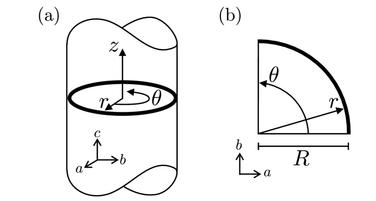
Figure 1: Surface (thick line) of the disk geometry, considered cut from an infinite cylinder with translational invariance along the crystal $c$-axis (a). Assuming at least $C_{4}$ symmetry this is reduced to a quarter disk (b) with $\theta=0$ and $\theta=\pi/2$ corresponding to the crystal $a$- and $b$-axis, respectively.

Polar coordinates: Polar coordinates $(r,\theta)$ are the natural choice for the disk geometry, where $r\in[0,R]$ and $\theta\in[0,\pi/2)$, defining $\theta=0$ and $\theta=\pi/2$ as the crystal $a$- and $b$-axis, respectively. Assuming translational invariance along the $c$-axis, the corresponding gradient term ($K_{5}$) in the free energy functional can be ignored such that $\boldsymbol{\eta}(\boldsymbol{r})=\boldsymbol{\eta}(r,\theta)$. The vector potential is $\boldsymbol{A}(\boldsymbol{r})=(A_{r}(r,\theta),A_{\theta}(r,\theta),0)=(A_{\perp}(r,\theta),A_{\parallel}(r,\theta),0)$ for a specific choice of gauge and the magnetic field only has a $z$-component $\boldsymbol{B}(\boldsymbol{r})=B_{z}(r,\theta)\boldsymbol{\hat{z}}$.

For the order parameter it is also convenient to turn to the polar representation $\boldsymbol{\eta}=(\eta_{r},\eta_{\theta})$, which is rewritten using the components being perpendicular and parallel to the surface, $\eta_{r}\to\eta_{\perp}$ and $\eta_{\theta}\to\eta_{\parallel}$, with

$$\boldsymbol{\eta} =(\eta_{\perp},\eta_{\parallel})=(\boldsymbol{n}\cdot\boldsymbol{\eta},\left(\boldsymbol{n}\times\boldsymbol{\eta}\right)\cdot\boldsymbol{\hat{z}})$$ (10)

$$=(\eta_{x}\cos\theta+\eta_{y}\sin\theta,-\eta_{x}\sin\theta+\eta_{y}\cos\theta).$$

Within this notation the real-space phase winding number $N=\pm 1$ for the two degenerate chiralities is introduced as $\boldsymbol{\eta}=(\eta_{\perp},\eta_{\parallel})=\eta_{\rm b}(u,iv)e^{iN\theta}$ with the still complex functions $u$ and $v$ of $(r,\theta)$. In the homogeneous bulk phase, $(\eta_{\perp},\eta_{\parallel})=\eta_{\rm b}(1,\pm i)e^{\pm i\theta}$. For an isotropic system $u=u(r)$ and $v=v(r)$ have no angular dependence.

Boundary conditions: For the disk geometry with $\boldsymbol{n}=\boldsymbol{\hat{r}}=(\cos\theta,\sin\theta)$ and using the above representation for the order parameter, the surface term from Eq. (6) is rewritten as

$$\mathcal{F}_{\mathrm{surf}} [\eta_{\perp},\eta_{\parallel}]=\int R\mathrm{d}\theta\bigg{[}g_{1}|\boldsymbol{\eta}|^{2}$$ (11)

$$+\left(g_{3}\cos^{2}(2\theta)+\frac{g_{4}}{2}\sin^{2}(2\theta)\right)\left(|\eta_{\perp}|^{2}-|\eta_{\parallel}|^{2}\right)$$

$$-\left(g_{3}-\frac{g_{4}}{2}\right)\sin(2\theta)\cos(2\theta)\left(\eta_{\perp}^{*}\eta_{\parallel}+\eta_{\perp}\eta_{\parallel}^{*}\right)\bigg{]}.$$

In order to reduce the number of variable system parameters, we insert the relation $g_{3}=g_{4}/2$, strictly valid only for isotropic symmetry. This leads to the simple form

$$\mathcal{F}_{\mathrm{surf}}[\eta_{\perp},\eta_{\parallel}]=\int R\mathrm{d}\theta\Big{[}(g_{1}+g_{3})|\eta_{\perp}|^{2}+(g_{1}-g_{3})|\eta_{\parallel}|^{2}\Big{]},$$ (12)

which we will use in the following for the boundary conditions. In the free energy functional, it is implemented straightforwardly by introducing an $r$-dependent critical temperature

$$T_{ci}^{\mathrm{eff}}(\boldsymbol{r})=T_{c}-T_{ci}\delta\left(r-R\right)$$ (13)

for the two order parameter components, with

$$T_{c\perp}=\frac{g_{1}+g_{3}}{a},\quad T_{c\parallel}=\frac{g_{1}-g_{3}}{a},$$ (14)

assuming that for $r>R$ there is vacuum. For the magnetic field, the boundary condition is $B_{z}(R,\theta)=0$.

II.4 Computational Method

The GL free energy functional is minimized numerically using a one-step relaxed Newton-Jacobi methodGardan (1985); Ortega and Rheinboldt (2000); Piette (2004); Etter (2017), for which the indirect boundary conditions through the effective critical temperatures can be implemented straightforwardly by changing the critical temperature at the surface of the disk according to the values of $g_{i}$ described in the next section. Both the order parameter and the vector potential are discretized on a regular polar grid with uniform step size and with $n=m=100$ mesh points for the radial and azimuthal coordinate, respectively. The fact that the tetragonal symmetry is kept in general, including the $C_{4}$ rotation, allows a restriction of our calculation to a quarter disk subject to periodic boundary conditions in the angular direction. In the radial direction, the origin is excluded by a circle of radius $r_{\mathrm{min}}=10\xi_{0}$. The disk radius is chosen to be $R=40\xi_{0}$, which for Sr₂RuO₄ would be a few $\mu$m in sizeMaeno et al. (2012). The gauge is chosen by fixing the order parameter values $\boldsymbol{\eta}=\eta_{0}(1,+i)$ and the vector potential $\boldsymbol{A}=0$ at $r_{\mathrm{min}}$, far enough away from the surface such that all quantities are constant. In certain limits analytical arguments allow us a comparison with the numerical results which in all cases agree very well. Also, the results from previous theoretical work are recovered where applicable.

III Range of system parameters

To explore the behavior of the surface magnetic flux pattern under various conditions, two essential parameter sets have been identified which we will scan systemtically. The ratio $K_{1}/K_{2}$ incorporates effects of the lattice on the electronic structure, while $g_{1}$ and $g_{3}$ cover a range of different surface types. Based on these parameters the different types of systems are defined and compared with previous studies.

Motivated by the results in Ref. [Bouhon and Sigrist, 2014], the ratio $K_{1}/K_{2}$ is scanned between the isotropic limit $K_{1}/K_{2}=3$ through $K_{1}=K_{2}$ to the ‘inverted’ ratio $K_{1}/K_{2}=1/3$. In this way the feature of current reversalBouhon and Sigrist (2014) can be reproduced for certain boundary conditions. While changing $K_{1}/K_{2}$ has been discussed before, the range of $K_{1}<K_{2}$ has not been studied within the GL approach so farAshby and Kallin (2009); Lederer et al. (2014). For our analysis, the difference $(K_{1}-K_{2})/K$ is varied rather than the ratio, as it turns out that the magnetic flux pattern depends on this difference, which can be seen for example from Eq. (35b).

Implementing the boundary conditions through the effective critical temperatures at the surface given in Eq. (14), the condition $T_{ci}\geq 0$ describes the destructive effect of the surface on superconductivity in general and leads to $g_{1}\geq|g_{3}|$. The restriction $T_{c\perp}\geq T_{c\parallel}$ further excludes scenarios where the parallel component of the order parameter would be suppressed more and leads to $g_{3}\geq 0$. The values $g_{1}=g_{3}=0$ describe a ‘virtual boundary’ in the interior of the superconductor without any effect on the order parameter. These requirements result in the area $G=\left\{g_{i}\ |\ (g_{1}\geq g_{3}\geq 0)\ \wedge\ (g_{1}+g_{3}>0)\right\}$, corresponding to the region shaded gray in Fig. 2.

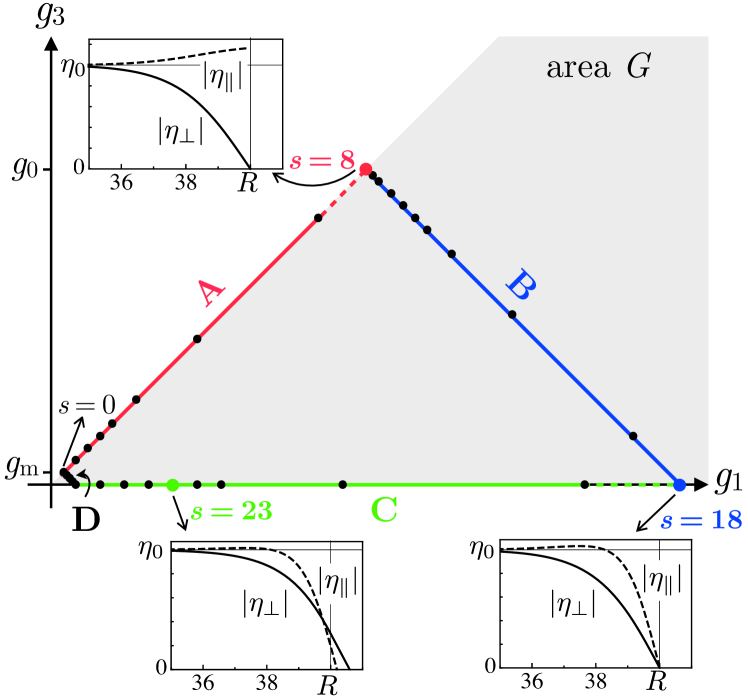
Figure 2: The area $G$ of the surface coefficients $g_{1}$ and $g_{3}$ covering the effective critical temperatures $T_{c\perp}^{\mathrm{eff}}\leq T_{c\parallel}^{\mathrm{eff}}\leq T_{c}$. The numerical analysis includes 31 cases $s$ (black dots) on the three ranges A, B, and C, and on D to exclude the origin. Three representative surface types are highlighted.

In the following, we focus on surface types along the ranges A, B, and C, the bounds of the area $G$, and introduce an additional range D to circumvent the origin, all indicated in Fig. 2. For the numerical analysis, the results are systematically computed for 31 cases $s\in\{0,\dots,30\}$, indicated by black dots, and whose actual values are listed in the supplemental materialsup . Three representative cases of particular interest are highlighted and illustrated by insets. The range A along the identity $g_{1}=g_{3}$ corresponds to surfaces with specular scattering. With $T_{c\parallel}=0$, the order parameter component $\eta_{\parallel}$ is little affected, as in Ref. [Matsumoto and Sigrist, 1999], while $T_{c\perp}$ grows with increasing $g_{i}$ and leads to a progressive suppression of $\eta_{\perp}$ at the surface, for which $\eta_{\parallel}$ is even slightly enhanced. The case $s=8$ corresponds to the limit $g_{1,3}=g_{0}\to\infty$ where the extrapolation length $l_{\perp}\ll\xi_{0}$ such that $\eta_{\perp}(R,\theta)\rightarrow 0$. For the numerical treatment, whenever $T_{ci}^{\mathrm{eff}}\rightarrow-\infty$, the direct boundary conditions $\eta_{i}(R)=0$ are implemented instead, as described in the supplemental materialsup . The range B, defined by $g_{1}+g_{2}=2g_{0}$, keeps $\eta_{\perp}$ fully suppressed at the boundary, whereby also $\eta_{\parallel}$ is reduced with decreasing $g_{3}$. For the case $s=18$, where $g_{3}=0$, both order parameter components vanish completely at the boundary. In range C, both order parameter components remain reduced but with finite extrapolations lengths. Both B and C describe effects due to surface roughness and diffuse scattering.

Before systematically analyzing the solution to our GL model, we briefly comment on the previous theoretical discussion of surface types. The commonly investigated situations are planar surfaces with specular scattering. Assuming full rotation symmetry around the $c$-axis, i.e. an isotropic system, a peak value for edge current induced fields of the order of 1 mT has been obtainedMatsumoto and Sigrist (1999), which is often used in experimental investigations in Sr₂RuO₄ as a referenceKirtley et al. (2007); Hicks et al. (2010); Curran et al. (2014). This case corresponds to our results at $s=8$ for $K_{1}/K_{2}=3$ with $\eta_{\perp}=0$ at the boundary. While our approach also covers ranges with finite $\eta_{\perp}$, most treatments impose the condition of its full suppression following the pioneering work by Ambegaokar, de Gennes and Rainer Ambegaokar et al. (1974). These studies are therefore located along the line BHuang and Yip (2012); Nagato et al. (1998); Ashby and Kallin (2009). Ashby and KallinAshby and Kallin (2009) considered the special case of ‘diffuse’ scattering with an extrapolation length $l_{\perp}=0.54$ following the results of Ref. [Ambegaokar et al., 1974], which is $s\approx 11$ in our discussion. Their analysis also includes ‘full pair breaking’ at the surfaceAshby and Kallin (2009), which here is $s=18$. While these works have considered planar surfaces, disk geometries with rather small radius have been studied by Huang and YipHuang and Yip (2012) and Suzuki and AsanoSuzuki and Asano (2016). On the other hand, normal metallic surface layers lead to a further type of boundary condition with finite extrapolation lengths for both order parameter components, as discussed previously by Lederer et al.Lederer et al. (2014). These authors considered also the special case of $K_{1}=K_{2}$ and identical extrapolation lengths, $l_{\perp}=l_{\parallel}$. Very recently, Bakurskiy et al.Bakurskiy et al. (2017) have extended the discussion to different surface layers of varying roughness and metallic behavior. These two works are covered by our analysis of range C.

IV Detailed Analysis

In this section, the spontaneous magnetic flux distribution generated by the surface currents is systematically analyzed. Starting with the isotropic limit, the ratio $K_{1}/K_{3}=3$ is fixed while the boundary conditions are changed. Then, restricted to specular scattering at the surface, anisotropy is introduced by varying $K_{1}/K_{3}$ between $3$ and $1/3$. Eventually, all surface types $s$ and all ratios $K_{1}/K_{2}$ are scanned and discussed systematically. The full set of numerical results can be found in the supplemental materialsup , while a selective analysis comprising the most essential features is given in this section.

IV.1 Different surface types in the isotropic limit

In the isotropic limit, $K_{1}/K_{2}=3$, all quantities such as the order parameter and the magnetic flux pattern have no angular dependence. The numerical results are shown in Fig. 3 for the three representative surface types highlighted in Fig. 2: specular scattering ($s=8$), full pair breaking ($s=18$) and the case of a rough surface with moderate pair breaking ($s=23$).

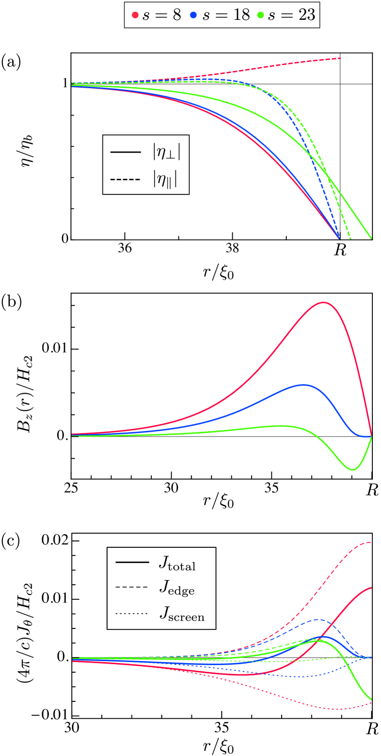
Figure 3: Numerical results for the three surface types specular scattering ($s=8$), full pair breaking ($s=18$) and a rough surface ($s=23$) in the isotropic limit. (a) The absolute value of the order parameter components $\eta_{\perp}$ and $\eta_{\parallel}$. (b) The magnetic flux $B_{z}$. (c) The total current at the surface $J_{\parallel}$, separated into the ‘edge’ and ‘screening’ part.

The order parameter components $\eta_{\perp}(r)$ and $\eta_{\parallel}(r)$ are displayed in Fig. 3(a). In the absence of angular dependence the global phase can be set constant with $\Im\eta_{\perp}=0$ and $\Re{\eta_{\parallel}}=0$. It is worth noting that for specular scattering $\eta_{\parallel}$ has an increasing slope at $r=R$, unlike on a planar surface, because the curvature supports this order parameter component, as demonstrated in Eq. (32a) in Appendix B.2, also in agreement with Suzuki and AsanoSuzuki and Asano (2016). For $s=18$ both components are suppressed to zero and for $s=23$ they are reduced at the surface with a finite extrapolation length on the order of the coherence length.

The magnetic field $B_{z}(r)$ due to edge currents is shown in Fig. 3(b). Specular scattering leads to a single positive peak near the surface, as found in Refs. [Matsumoto and Sigrist, 1999] and [Ashby and Kallin, 2009]. A similar peak structure appears also for $s=18$, however, with a reduced magnitude, in agreement with Ref. [Ashby and Kallin, 2009]. A qualitative change occurs for $s=23$ where $B_{z}$ changes sign, starting negative near the surface and crossing to positive at a distance on the order of the coherence length. Interestingly, the total flux of this case is essentially zero. Note that this corresponds to a node of the $s$-dependence of the magnetic flux, as $s=22$ and $s=24$ have a finite total flux of opposite sign (see Fig. 7(b)).

The surface current $J_{\parallel}$ is depicted in Fig. 3(c), while the radial current $J_{\perp}$ vanishes everywhere in the isotropic limit. It is illustrative to separate the current into two parts, the driving current due to the edge, $J_{\rm edge}$, and the screening current to suppress the magnetic field inside the disk, $J_{\rm screen}$, for the definition see Eq. (34) in Appendix B.2. The spatial extension of these currents has different length scales, the coherence length for $J_{\rm edge}$ and the London penetration depth for $J_{\rm screen}$. Note that these lengths are similar due to the small Ginzburg-Landau parameter $\kappa=2.6$. Again, the driving currents for $s=8$ and 18 are both positive, but the latter is reduced compared to the former and vanishes at the surface, as shown by Eq. (36) in Appendix B.2. The current for $s=23$ has a sign change and correspondingly the screening current is strongly reduced.

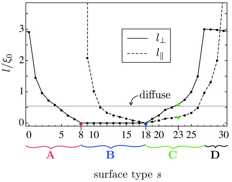
Figure 4: Extrapolation lengths $l_{\perp}$ (solid) and $l_{\parallel}$ (dashed) of the order parameter components in the isotropic limit for all surface types. The ranges A, B, C, and D, the three representative cases $s\in\{8,18,23\}$ (see Fig. 2), as well as the specific extrapolation length $l_{\mathrm{diff}}=0.54$ are indicated.

In the isotropic limit it is also interesting to consider the extrapolation lengths $l_{\perp}$ and $l_{\parallel}$ for $\eta_{\perp}$ and $\eta_{\parallel}$, respectively, which can be extracted from the numerical results and shown in Fig. 4. For the specular scattering surface types in range A (see Fig. 2), $l_{\parallel}$ diverges, while $l_{\perp}$ decreases as $\eta_{\perp}$ is progressively suppressed at the surface starting at $s=0$ until $l_{\perp}=0$ for $s=8$. Within range B, $\eta_{\perp}$ remains zero at the surface such that $l_{\perp}=0$. The gradual suppression of $\eta_{\parallel}$ leads to a decrease of $l_{\parallel}$ until it vanishes at $s=18$ with full pair breaking. For range C, both extrapolation lengths increase again continuously with $3l_{\parallel}\sim l_{\perp}$ due to the difference in coherence length for the two order parameter components, see Eq. (31) in Appendix B.2. Along range D, $l_{\perp}$ basically remains constant, while $l_{\parallel}$ grows to eventually diverge again at $s=0$.

The specific extrapolation length $l_{\mathrm{diff}}=0.54$ is also indicated, which describes the ‘diffuse’ scattering as derived by Ambegaokar, de Gennes and RainerAmbegaokar et al. (1974) and treated within a GL approach by Ashby and KallinAshby and Kallin (2009). Our boundary condition $s=11$ is very close to this case and the corresponding results are in agreement with Ref. [Ashby and Kallin, 2009].

IV.2 Specular scattering and anisotropy

Turning $K_{1}/K_{2}$ away from 3 introduces anisotropy such that all quantities acquire angular dependence. Here we restrict our discussion to the specular scattering surface type $s=8$. The magnetic flux pattern for different ratios $K_{1}/K_{2}$ is displayed in Fig. 5, starting with the isotropic limit $K_{1}/K_{2}=3$ (upper left) to $K_{1}/K_{2}=1/3$ (lower right). Due to the assumed $C_{4}$ symmetry, it is sufficient to display a quarter disk with $0\leq\theta\leq\pi/2$, where $\theta=0,\pi/2$ correspond to the crystalline axes of the basal plane.

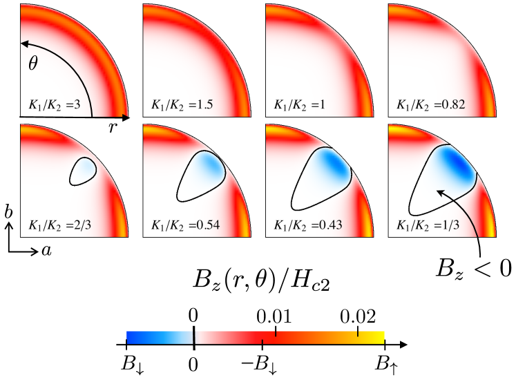
Figure 5: The magnetic flux $B_{z}$ for the specular scattering surface type $s=8$ at different ratios $K_{1}/K_{2}$. Negative fluxes are blue, with deep blue being the minimum $B_{\downarrow}$, and encircled by a thick black line. The corresponding positive value $-B_{\downarrow}$ is colored deep red and the maximum $B_{\uparrow}$ is yellow. The subplot $K_{1}/K_{2}=1/3$ (bottom right) is enlarged in Fig. 6.

The magnetic flux pattern for $K_{1}/K_{2}=3$ agrees with the result shown in Fig. 3(b) for $s=8$. Lowering $K_{1}/K_{2}$ the flux pattern progressively develops anisotropy. In agreement with Ashby and KallinAshby and Kallin (2009), the magnetic flux increases along the [10]-directions $\theta=0$ and $\pi/2$. On the other hand, it decreases along the [11]-direction $\theta=\pi/4$. When the ratio is $K_{1}/K_{2}\approx 2/3$ in this direction, a slightly negative flux region appears (encircled by a black line) which expands upon decreasing $K_{1}/K_{2}$. This behavior is consistent with the observation of current reversal by Bouhon and Sigrist within a lattice BdG approach for a planar surface along the [11]-directionBouhon and Sigrist (2014). The current pattern is shown in the more detailed plot for the ‘inverted’ ratio $K_{1}/K_{2}=1/3$ in Fig. 6, where the surface currents run in a clockwise direction for $\theta=0$ and $\pi/2$, and anti-clockwise for $\theta=\pi/4$. Interestingly, the critical ratio for the onset of the current reversal is lower for the curved than for a planar surface, as discussed for Eq. (35) in Appendix B.2. Increasing the disk radius to $R=240\xi_{0}$, we observe the negative flux and surface currents at higher ratios, closer to $K_{1}=K_{2}$.

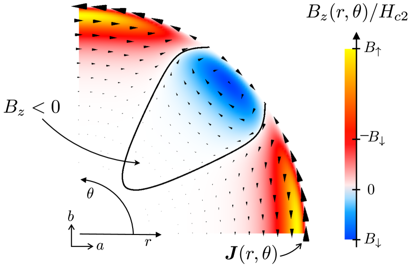
Figure 6: Density plot of the magnetic flux $B_{z}$ and a scaled vector plot of the current $\boldsymbol{J}$ for the inverted ratio $K_{1}/K_{2}=1/3$ and the specular scattering surface $s=8$. The current pointers are scaled by $|\boldsymbol{J}|^{1/3}$ to enhance the small values.

IV.3 Full scan of parameters

Finally, the flux pattern is analyzed for the whole range of surface types and ratios $K_{1}/K_{2}$. Selected quantities extracted from the numerical results are presented in Fig. 7 as density plots with $s$ along the horizontal and $K_{1}/K_{2}$ along the vertical axis. Note that the vertical scale is non-linear because equal steps are taken in $(K_{1}-K_{2})/K$. A useful symmetry relation for the magnetic field is explained in Appendix B.1,

$$B_{z}[K_{1}/K_{2},g_{1},g_{3}=0]=-B_{z}[K_{2}/K_{1},g_{1},g_{3}=0].$$ (15)

In particular, it establishes the observation that the magnetic flux vanishes for $K_{1}=K_{2}$ and $g_{3}=0$ (range C), see also Ref. [Lederer et al., 2014].

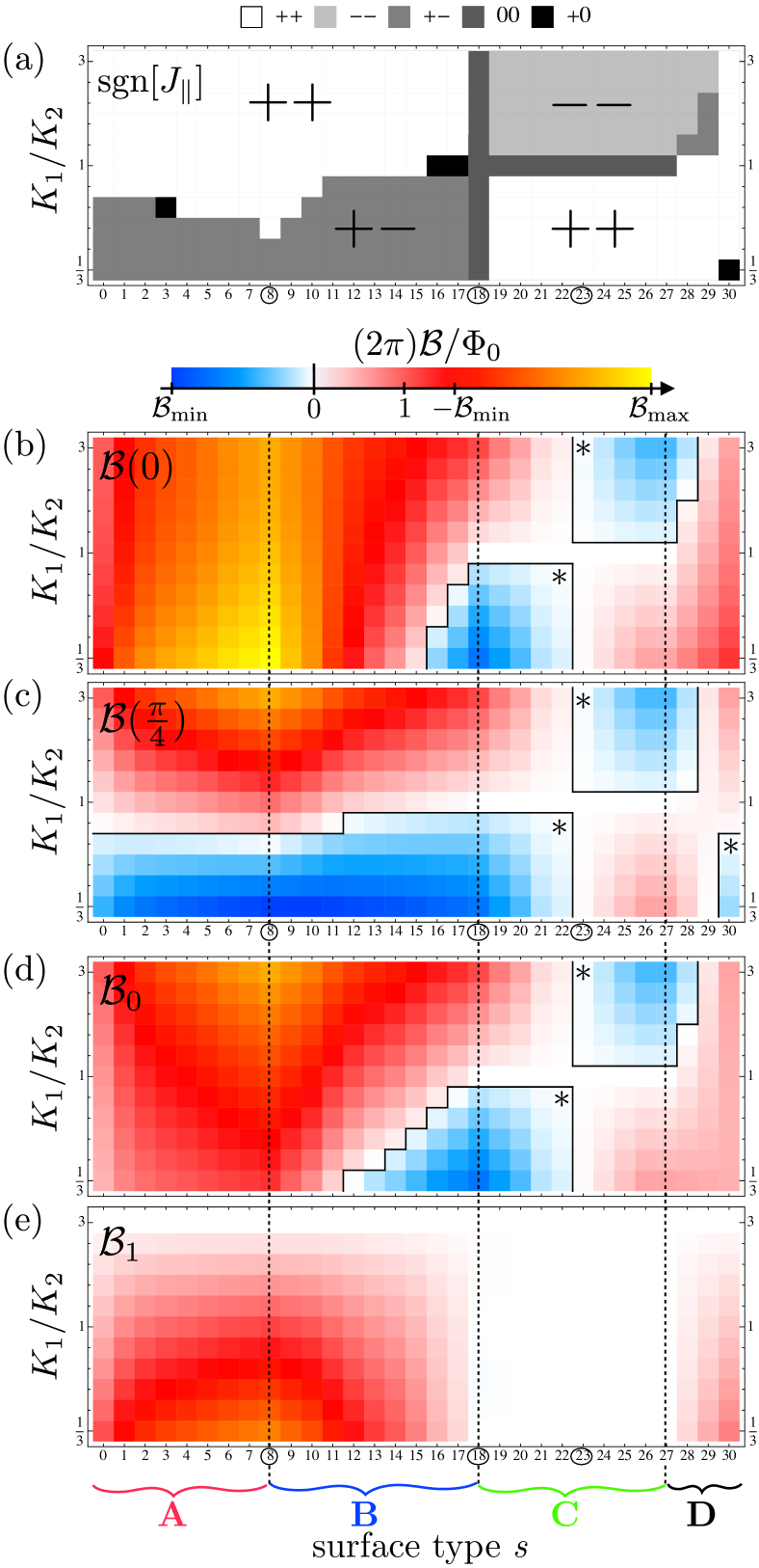
Figure 7: Extracted quantities: (a) the current directions $\{\mathrm{sgn}J_{\parallel}(0),\mathrm{sgn}J_{\parallel}(\pi/4)\}$; the radially integrated flux $\mathcal{B}(\theta)$ at (b) $\theta=0$ and (c) $\theta=\pi/4$; (d) the total flux $\mathcal{B}_{0}=\Phi/(2\pi)$, and (e) the first component of the Fourier analysis $\mathcal{B}_{1}$. The color scale ranges from the overall minimum $\mathcal{B}_{\mathrm{min}}<0$ (deep blue) through the corresponding positive value (deep red) to the overall maximum $\mathcal{B}_{\mathrm{max}}>0$ (yellow). Areas of negative $\mathcal{B}$ are encircled by a black line and labeled $*$.

First, the direction of the surface current for the surface orientations $\theta=0$ and $\pi/4$ is analyzed in Fig. 7(a), considering only the signs $\{\mathrm{sgn}[J_{\parallel}(\theta=0)],\mathrm{sgn}[J_{\parallel}(\theta=\pi/4)]\}$. For surface types A and B, the current $J_{\parallel}(\theta=0)$ is positive for all ratios $K_{1}/K_{2}$. On the other hand, the current $J_{\parallel}(\theta=\pi/4)$ changes sign at a value $K_{1}/K_{2}<1$ varying moderately with the surface type $s$. At $s=18$, the surface current vanishes for all ratios $K_{1}/K_{2}$, see Eq. (36) in Appendix B.2, with the onset pushed inside the disk as illustrated in Fig. 7(c). For range C, the surface current starts in the isotropic limit with negative values for both surface orientations. In agreement with the symmetry relation in Eq. (15), the current vanishes identically for the whole disk at $K_{1}=K_{2}$ and changes direction for $K_{1}<K_{2}$.

More insight into the behavior of the magnetic flux pattern is obtained by considering the angular dependence after integrating over the radial direction,

$$\mathcal{B}(\theta)=\int r\mathrm{d}rB_{z}(r,\theta).$$ (16)

This is analyzed successively in Figs. 7(b)-(e), where the same color scale is used in all subplots for an easy comparison, with $\mathcal{B}_{\mathrm{min}}$ and $\mathcal{B}_{\mathrm{max}}$ being the overall extremal values, occurring as discussed below. First, we discuss $\mathcal{B}(\theta)$ for the orientations $\theta=0$ and $\pi/4$ in Figs. 7(b) and (c), respectively. In range A and B, $\mathcal{B}(0)$ is positive with the overall maximum $\mathcal{B}_{\mathrm{max}}$ reached for the specular scattering case $s=8$ and the most pronounced anisotropy $K_{1}/K_{2}=1/3$. The characteristic feature of $\mathcal{B}(\pi/4)$ is the sign change at a ratio $K_{1}/K_{2}<1$. The overall minimum $\mathcal{B}_{\mathrm{min}}$ ($<0$) is reached for $s=8$ and $K_{1}/K_{2}=1/3$. The same pattern appears for both $\mathcal{B}(0)$ and $\mathcal{B}(\pi/4)$ in range C, with a vanishing flux when $K_{1}=K_{2}$, based on the symmetry relation in Eq. (15). For $s=23$, the flux vanishes for all ratios $K_{1}/K_{2}$.

Next, we examine the angular dependence of $\mathcal{B}(\theta)$ using the Fourier decomposition

$$\mathcal{B}(\theta)=\sum_{n=0}^{\infty}\mathcal{B}_{n}\cos(4n\theta).$$ (17)

The total magnetic flux through the disk is $\Phi=2\pi\mathcal{B}_{0}$ and shown in Fig. 7(d). The lowest order angular dependence $\mathcal{B}_{1}$ is shown in Fig. 7(e). Typically, we find $|\mathcal{B}_{n\geq 2}|\ll\{|\mathcal{B}_{0}|,|\mathcal{B}_{1}|\}$, such that higher orders can be neglected here. For $s$ in A and B, naturally $\mathcal{B}_{0}$ dominates in the more isotropic ($K_{1}>K_{2}$) and $\mathcal{B}_{1}$ in the more anisotropic ($K_{1}<K_{2}$) regime. Interestingly, the total flux $\mathcal{B}_{0}$ can also become negative in range B for a sufficiently pronounced anisotropy. The strongest angular dependence is obtained again for specular scattering at $s=8$ and the maximal anisotropy $K_{1}/K_{2}=1/3$. The magnetic flux pattern in range C is essentially isotropic $\mathcal{B}_{1}\approx 0$. Therefore, independent of the surface orientation, the magnetic flux vanishes for the case $s=23$ for all $K_{1}/K_{2}$ and for $K_{1}=K_{2}$ for all $s\in\{18,\dots,27\}$, the latter again based on the symmetry relation Eq. (15).

We conclude that the case of specular scattering gives rise to the largest magnetic fields. This ‘upper bound’ corresponds to the situation discussed in Ref. [Matsumoto and Sigrist, 1999] which is often taken as a reference for the magnitude of the spontaneous magnetic fields at the surface. It can be enhanced somewhat by anisotropy. We also reproduce the current reversal obtained by a lattice BdG approachBouhon and Sigrist (2014). Most surprising is the fact that the magnetic fields can be suppressed for all surface orientations in a wider range when the boundary conditions are sufficiently destructive. In particular, the vanishing total flux and the current reversal are not isolated and fine-tuned results, but appear for a larger range of parameters.

V Impurity

Besides boundaries, impurities also distort the order parameter in unconventional superconductors. Analogous to the surface, for chiral $p$-wave superconductors this leads to spontaneous currents circling around the impurity, inducing a local magnetic field. Within our GL framework the presence of a single isolated bulk impurity at $\boldsymbol{r}_{\mathrm{imp}}$ is easily implemented by a correction to the critical temperature,

$$T_{c}^{\mathrm{eff}}=T_{c}\big{(}1-\tau_{\mathrm{imp}}\delta(\boldsymbol{r}-\boldsymbol{r}_{\mathrm{imp}})\big{)},$$ (18)

where $\tau_{\mathrm{imp}}>0$ corresponds to the depletion strength of the order parameter, see also Ref. [Okuno et al., 1999]. As a quasi two-dimensional superconductor is considered, the coherence length along the $z$-direction is very short, such that the driving currents are well concentrated in the layer where the impurity is located and screening is mainly due to currents parallel to the basal plane. For simplicity, the discussion is restricted to a two-dimensional system. For the numerical analysis, a square with side length $L=30\xi_{0}$ is considered, with the point-like impurity located in the center. In analogy to the discussion above, the ratio $K_{1}/K_{2}$ again introduces anisotropy, while now the strength $\tau_{\mathrm{imp}}$ is the additional scanning parameter.

Figure 8: Magnetic flux pattern $B_{z}$ around an isolated impurity with strength $\tau_{\mathrm{imp}}=50\xi_{0}^{2}$ where the order parameter is fully suppressed, and in the isotropic limit. The colors red to yellow indicate increasing positive flux, while blue is the much smaller negative screening flux at larger distances. Again, the pointers are scaled by $|\boldsymbol{J}|^{1/3}$ to enhance small values.

The magnetic field and current distribution around the impurity are shown in Fig. 8 for the isotropic limit $K_{1}/K_{2}=3$ and for a strength $\tau_{\mathrm{imp}}$ at which the order parameter is fully suppressed in the center. The magnetic field is strongly peaked at the impurity site $r=0$ and is compensated by a negative tail at larger distances. The total magnetic flux $\Phi_{\mathrm{imp}}$ vanishes as required. The magnitude of the flux peak $B_{\mathrm{peak}}$ depends both on the ratio $K_{1}/K_{2}$ and on the strength $\tau_{\mathrm{imp}}$, as shown in Fig. 9. The two effects are considered separately. First, the effect of the strength $\tau_{\mathrm{imp}}$ is shown in Fig. 9(a) for the isotropic limit $K_{1}/K_{2}=3$. At a large enough value of $\tau_{\mathrm{imp}}$, both order parameter components are fully suppressed at the site of the impurity, and the peak strength $B_{\mathrm{peak}}$ saturates. Second, the effect of the anisotropy from scanning the ratio $K_{1}/K_{2}$ is shown in Fig. 9(b) for a value of $\tau_{\mathrm{imp}}$ where $B_{\mathrm{peak}}$ has saturated in the isotropic limit. Equal steps in $(K_{1}-K_{2})/K$ are taken. The odd dependence of $B_{\mathrm{peak}}$ on $(K_{1}-K_{2})/K$ is in agreement with the symmetry relation from Eq. (15), which also applies here. The peak magnitude is essentially linear in $(K_{1}-K_{2})/K$.

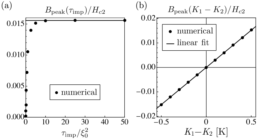
Figure 9: Dependence of the magnitude of the flux peak $B_{\mathrm{peak}}$ on (a) the strength $\tau_{\mathrm{imp}}$ in the isotropic limit; and on (b) the ratio $K_{1}/K_{2}$ ($K_{1}-K_{2}=0.5K$ corresponds to the isotropic limit) for an impurity with a strength $\tau_{\mathrm{imp}}=10\xi_{0}^{2}$ where the order parameter is fully suppressed and $B_{\mathrm{peak}}$ has saturated.

VI Conclusion

The aim of our study was to illustrate the variability of the spontaneous magnetic flux pattern $B_{z}(r,\theta)$ at the surface of a chiral $p$-wave superconductor. The disk geometry provides a sample including all surface orientations. The Ginzburg Landau approach allows us to examine a wide range of conditions, in particular, different boundary conditions and the anisotropy of the electronic structure due to the crystal lattice. For the purpose of a systematic scan of these conditions for a given chirality, the relevant ‘anisotropy’ parameter $K_{1}/K_{2}$ was introduced and an extensive set of surface types labeled by $s$ was chosen, while ignoring the variability of other parameters in the GL functional. We compared our results with those of previous studies and could reproduce these results as special cases of our more extensive discussion. In particular, we verified also the somewhat counter-intuitive current reversal around the direction [110] found in Ref. [Bouhon and Sigrist, 2014].

Our main result is that the flux pattern is not a universal feature of the topologically non-trivial chiral superconducting phase, but it is extremely sensitive to both the ratio $K_{1}/K_{2}$ and the surface type $s$, in combination with the surface orientation. This is apparent immediately on the chart of all flux patterns provided in the supplemental materialsup . The naive picture of a chiral superconductor to behave like an orbital ferromagnet where edge currents are considered as uncompensated circular currents does definitely not conform with our findings. Not only the magnitude of $B_{z}(r,\theta)$ varies, but it can also be highly anisotropic and even change sign. Only a specular scattering surface in the isotropic limit conforms well with the naive expectation. There is a certain range of conditions where the magnetic flux vanishes completely. Interestingly, the magnetic flux at an impurity follows a behavior similar to the flux at the surface along range C concerning the dependence on $K_{1}/K_{2}$. Additionally, however, the peak strength at the impurity is governed by the phenomenological parameter $\tau_{\mathrm{imp}}$, and saturates when both order parameter components are fully suppressed.

We also considered the radially integrated flux and found that there are parameter ranges where this quantity vanishes due to cancellation, although the local magnetic fields are non-vanishing. Since the extension of the flux pattern from the surface is limited to a length of order of the London penetration depth, this fact may also be relevant for experimental detection by devices which have a considerably coarser spatial resolution than this. On the other hand, experimental accuracy has improved considerably over the last few years making the limiting bound very restrictive for the possible range within our scan. Band structure discussions based on a BdG approachLederer et al. (2014); Bouhon and Sigrist (2014) suggest that for Sr₂RuO₄ the ratio $K_{1}/K_{2}<1$, which is far from the isotropic limit and even in the regime where current reversal can occur. Furthermore, real sample surfaces are most likely far from specular scattering, but rather belong to the limit of a rough surfaceLederer et al. (2014). While it remains difficult to reliably determine the parameters corresponding to a given sample of Sr₂RuO₄, we consider the analysis of the experimental results based on the expectations of a specular scattering surface in the isotropic limit as certainly not realistic.

Appendix A The Ginzburg-Landau expansion coefficients

In this appendix we provide an overview of the scheme to derive the relation between the different expansion coefficients in the Ginzburg-Landau free energy as given in Eq. (2). The chiral $p$-wave state belongs to the two-dimensional irreducible odd-parity representation $E_{u}$ of the tetragonal point group $D_{4h}$. The gap function in d-vector notation is in its most general form given by

$$\boldsymbol{d}(\boldsymbol{k})=\eta_{0}(\phi_{x}(\boldsymbol{k})\eta_{x}(\boldsymbol{r})+\phi_{y}(\boldsymbol{k})\eta_{y}(\boldsymbol{r}))\boldsymbol{\hat{z}}$$ (19)

where $\{\phi_{x}(\boldsymbol{k}),\phi_{y}(\boldsymbol{k})\}$ are the two basis functions of $E_{u}$. In a weak coupling approach and restricted to a single band (for Sr₂RuO₄ the $\gamma$-band as most dominant among the three bands), the coefficients of the fourth order terms of the free energy are obtained through

$$b_{1} =b\langle\phi_{x}^{4}\rangle_{\mathrm{FS}}$$ (20a)

$$b_{2} =2b\langle\phi_{x}^{2}\phi_{y}^{2}\rangle_{\mathrm{FS}}$$ (20b)

$$b_{3} =2(b_{2}-b_{1}),$$ (20c)

where $\langle\cdot\rangle_{\mathrm{FS}}$ is the average over the Fermi surface and $b$ is an appropriate parameter depending on specific material properties. For the gradient terms, the same procedure leads to

$$K_{1} =K\langle v_{x}^{2}\phi_{x}^{2}\rangle_{\mathrm{FS}}$$ (21a)

$$K_{2} =K\langle v_{y}^{2}\phi_{x}^{2}\rangle_{\mathrm{FS}}$$ (21b)

$$K_{3}=K_{4} =K\langle v_{x}v_{y}\phi_{x}\phi_{y}\rangle_{\mathrm{FS}},$$ (21c)

where $\boldsymbol{v}$ is the Fermi velocity and $K$ is a parameter analogous to $b$ .

In the isotropic limit, that is, for a rotationally symmetric system with a cylindrical Fermi surface of radius $k_{F}$, both the momentum and the Fermi velocity reduce to $\boldsymbol{k}=k_{F}(\cos\varphi,\sin\varphi)$ and $\boldsymbol{v}=v_{F}(\cos\varphi,\sin\varphi)$, and the basis functions can be chosen as $\phi_{i}(\boldsymbol{k})=k_{i}$. Taking the average over the Fermi surface by integration this directly leads to

$$b_{1}=\frac{3}{8}k_{F}^{4}b,\;\;b_{2}=-b_{3}=\frac{1}{4}k_{F}^{4}b$$ (22)

and

$$K_{1}=\frac{3}{8}v_{F}^{2}k_{F}^{2}K,\;\;K_{2}=K_{3}=K_{4}=\frac{1}{8}v_{F}^{2}k_{F}^{2}K.$$ (23)

This yields the ratios for the isotropic limit, frequently used above,

$$2b_{1}=3b_{2}=-3b_{3}$$ (24)

and

$$K_{1}=3K_{2}=3K_{3}=3K_{4}.$$ (25)

For further details we refer to Refs. [Etter, 2017] and [Bouhon, 2014].

Appendix B Selected analytic expressions

In this appendix, selected analytical expressions derived from the full Ginzburg Landau (GL) free energy functional are collected to enhance the arguments based on the numerical results.

B.1 Symmetry of the free energy functional

The free energy functional displays the symmetry

$$\mathcal{F}[\eta_{x},\eta_{y},D_{x},D_{y},K_{1},K_{2}]=\mathcal{F}[\eta_{x},\eta_{y},D_{y},D_{x},K_{2},K_{1}]$$ (26)

for any weak-coupling approach with $K_{3}=K_{4}$. This still holds for boundary conditions identical for both order parameter components, i.e. when the effective critical temperature is the same for both components, which includes all surface types with $g_{3,4}=0$ (range C) and the model of an impurity with locally reduced $T_{c}$. Note that switching $D_{x}$ and $D_{y}$ results in a sign change for the magnetic flux $B_{z}$, because $\varepsilon_{ijk}=-\varepsilon_{jik}$ in $\nabla\times\boldsymbol{A}$, such that $B_{z}(K_{1},K_{2})=-B_{z}(K_{2},K_{1})$. Including the requirements on the surface coefficients $g_{i}$, this leads to Eq. (15), which is confirmed for the surface types C and for an impurity.

B.2 Expressions derived by variation

For the disk geometry (radius $R$) it is convenient to use polar coordinates $\boldsymbol{r}=(r,\theta)$ and the polar representation of the order parameter components $\boldsymbol{\eta}=(\eta_{\perp},\eta_{\parallel})$ defined in Eq. (10), such that the full free energy is

$$\mathcal{F}\left[\eta_{\perp}(r,\theta),\eta_{\parallel}(r,\theta),A_{\perp}(r,\theta),A_{\parallel}(r,\theta)\right].$$ (27)

This lengthy expression is omitted here. Rather, the boundary conditions for the order parameters and the full expression for the angular current derived by variation are discussed below.

Boundary conditions for the order parameters

The boundary conditions (BC) from the variation with respect to the order parameter components $\eta_{\perp}$ and $\eta_{\parallel}$ are given below, where the space dependence $(R,\theta)$ is omitted for compactness of the expressions, and where $\widetilde{K}=(K_{1}-K_{2}-2K_{3})$.

$$\begin{split}&-4(g_{1}+g_{3})\eta_{\perp}=\left(3K_{1}+K_{2}+2K_{3}+\cos(4\theta)\widetilde{K}\right)\partial_{r}\eta_{\perp}\\ &\quad\quad+\left(K_{1}-K_{2}+2K_{3}-\cos(4\theta)\widetilde{K}\right)\left(\frac{\eta_{\perp}}{R}+\frac{\partial_{\theta}\eta_{\parallel}}{R}\right)-\sin(4\theta)\widetilde{K}\left(\frac{\partial_{\theta}\eta_{\perp}}{R}-\frac{\eta_{\parallel}}{R}+\partial_{r}\eta_{\parallel}\right)\\ &\quad\quad-i\gamma A_{\parallel}\left(\left(K_{1}-K_{2}+2K_{3}-\cos(4\theta)\widetilde{K}\right)\eta_{\parallel}-\sin(4\theta)\widetilde{K}\eta_{\perp}\right)\\ &\quad\quad-i\gamma A_{\perp}\left(\left(3K_{1}+K_{2}+2K_{3}+\cos(4\theta)\widetilde{K}\right)\eta_{\perp}-\sin(4\theta)\widetilde{K}\eta_{\parallel}\right),\end{split}$$ (28a)

$$\begin{split}&-4(g_{1}-g_{3})\eta_{\parallel}=\left(K_{1}+3K_{2}-2K_{3}-\cos(4\theta)\widetilde{K}\right)\partial_{r}\eta_{\parallel}\\ &\quad\quad-\left(K_{1}-K_{2}+2K_{3}-\cos(4\theta)\widetilde{K}\right)\left(\frac{\eta_{\parallel}}{R}-\frac{\partial_{\theta}\eta_{\perp}}{R}\right)+\sin(4\theta)\widetilde{K}\left(\frac{\partial_{\theta}\eta_{\parallel}}{R}+\frac{\eta_{\perp}}{R}-\partial_{r}\eta_{\perp}\right)\\ &\quad\quad-i\gamma A_{\parallel}\left(\left(K_{1}-K_{2}+2K_{3}-\cos(4\theta)\widetilde{K}\right)\eta_{\perp}+\sin(4\theta)\widetilde{K}\eta_{\parallel}\right)\\ &\quad\quad-i\gamma A_{\perp}\left(\left(K_{1}+3K_{2}-2K_{3}-\cos(4\theta)\widetilde{K}\right)\eta_{\parallel}-\sin(4\theta)\widetilde{K}\eta_{\perp}\right).\end{split}$$ (28b)

Three special cases are discussed further, straight surfaces at the angles $\theta=\{0,\pi/4\}$, the isotropic limit $K_{1}/K_{2}=3$, and the specular scattering surface type $s=8$.

The limit of a straight surface is $R\rightarrow\infty$ and $A_{\perp}=0$ for a choice of gauge. At $\theta=0$, Eq. (7) is recovered,

$$-(g_{1}+g_{3})\eta_{x}=K_{1}\partial_{x}\eta_{x}-i\gamma A_{y}K_{3}\eta_{y}$$ (29a)

$$-(g_{1}-g_{3})\eta_{y}=K_{2}\partial_{x}\eta_{y}-i\gamma A_{y}K_{3}\eta_{x}.$$ (29b)

For comparison, at the angle $\theta=\pi/4$, the BCs are

$$\begin{split}&-2(g_{1}+g_{3})\eta_{\perp}=\\ &\quad\big{(}K_{1}+K_{2}+2K_{3}\big{)}\partial_{n}\eta_{\perp}-i\gamma A_{\parallel}\big{(}K_{1}-K_{2}\big{)}\eta_{\parallel}\end{split}$$ (30a)

$$\begin{split}&-2(g_{1}-g_{3})\eta_{\parallel}=\\ &\quad\big{(}K_{1}+K_{2}-2K_{3}\big{)}\partial_{n}\eta_{\parallel}-i\gamma A_{\parallel}\big{(}K_{1}-K_{2}\big{)}\eta_{\perp}.\end{split}$$ (30b)

In the isotropic limit we have $\widetilde{K}=0$, and for a proper choice of gauge the angular dependence can be written as $\boldsymbol{\eta}=(\eta_{\perp},\eta_{\parallel})=\eta_{\rm b}(u(r),iv(r))e^{iN\theta}$, with $A_{\parallel}(r,\theta)=A_{\parallel}(r)$ and $A_{\perp}=0$, such that

$$-4(g_{1}+g_{3})\eta_{\perp}=3K\partial_{r}\eta_{\perp}+K\frac{\eta_{\perp}}{R}-i\left(\gamma A_{\parallel}-\frac{N}{R}\right)K\eta_{\parallel}$$ (31a)

$$-4(g_{1}-g_{3})\eta_{\parallel}=K\partial_{r}\eta_{\parallel}-K\frac{\eta_{\parallel}}{R}-i\left(\gamma A_{\parallel}-\frac{N}{R}\right)K\eta_{\perp}.$$ (31b)

For the specular scattering surface type $s=8$, the perpendicular component is fully suppressed at the surface, $\eta_{\perp}(R)=0$. While for straight surfaces (limit $R\to\infty$) the parallel component $\eta_{\parallel}$ has a vanishing slope at the surface, the slope is finite for curved surfaces with finite $R$. At the angle $\theta=0$, the slope is given by

$$K_{2}\partial_{r}\eta_{\parallel}\Big{|}_{R}=K_{3}\frac{\eta_{\parallel}(R)}{R},$$ (32a)

and at the angle $$\theta=\pi/4$$ by

$$(K_{1}+K_{2}-2K_{3})\partial_{r}\eta_{\parallel}\Big{|}_{R}=(K_{1}-K_{2})\frac{\eta_{\parallel}(R)}{R},$$ (32b)

where we have used the fact that symmetry arguments lead straightforwardly to $A_{\perp}(\theta=0)=A_{\perp}(\theta=\pi/4)=0$ for our choice of gauge, as described in Ref. [Etter, 2017]. In the isotropic limit as described above, this results in a positive slope at all angles (see Fig. 3(a)). Away from the isotropic limit, the slope at $\theta=0$ always remains positive, while the slope at $\theta=\pi/4$ vanishes when $K_{1}=K_{2}$ and changes sign for $K_{1}<K_{2}$. We further note that these equations even hold for concave surfaces, but that due to the negative curvature the slope has opposite sign at the surface, leading for example to a slight reduction of $\eta_{\parallel}$ at the surface in the isotropic limit. In any case, the initial enhancement of the parallel order parameter due to the suppression of the perpendicular component always remains and dominates the overall behavior.

Full expression for the angular current

The full GL equation for the parallel current $J_{\parallel}(r,\theta)$ (not restricted to the surface) derived by variation is given below, where the space dependence $(r,\theta)$ is again omitted for compactness of the expressions, and where again $\widetilde{K}=(K_{1}-K_{2}-2K_{3})$.

$$\begin{split}-\frac{2}{c\gamma}J_{\parallel}=&\left(K_{1}-K_{2}+2K_{3}\right)\Im\left[\eta_{\perp}\partial_{r}\eta_{\parallel}^{*}-\partial_{r}\eta_{\perp}\eta_{\parallel}^{*}\right]\\ &-\frac{1}{r}\Im\left[\left(4\left(K_{1}+K_{2}\right)\eta_{\perp}\eta_{\parallel}^{*}-\left(K_{1}+3K_{2}-2K_{3}\right)\eta_{\perp}\partial_{\theta}\eta_{\perp}^{*}-\left(3K_{1}+K_{2}+2K_{3}\right)\eta_{\parallel}\partial_{\theta}\eta_{\parallel}^{*}\right)\right]\\ &-\widetilde{K}\Im\left[\eta_{\perp}\partial_{r}\eta_{\parallel}^{*}-\partial_{r}\eta_{\perp}\eta_{\parallel}^{*}+\frac{1}{r}\left(\eta_{\perp}\partial_{\theta}\eta_{\perp}^{*}-\eta_{\parallel}\partial_{\theta}\eta_{\parallel}^{*}\right)\right]\cos(4\theta)\\ &-\widetilde{K}\Im\left[\eta_{\perp}\partial_{r}\eta_{\perp}^{*}-\eta_{\parallel}\partial_{r}\eta_{\parallel}^{*}-\frac{1}{r}\left(\eta_{\perp}\partial_{\theta}\eta_{\parallel}^{*}-\partial_{\theta}\eta_{\perp}\eta_{\parallel}^{*}\right)\right]\sin(4\theta)\\ &+\gamma A_{\perp}\left(\left(K_{1}-K_{2}+2K_{3}-\cos(4\theta)\widetilde{K}\right)2\Re\left[\eta_{\perp}\eta_{\parallel}^{*}\right]-\sin(4\theta)\widetilde{K}\left(|\eta_{\perp}|^{2}-|\eta_{\parallel}|^{2}\right)\right)\\ &+\gamma A_{\parallel}\Big{(}2\left(K_{1}+K_{2}\right)|\boldsymbol{\eta}|^{2}-\left(K_{1}-K_{2}+2K_{3}\right)\left(|\eta_{\perp}|^{2}-|\eta_{\parallel}|^{2}\right)\\ &\quad\quad\quad\,\,-\cos(4\theta)\widetilde{K}\left(|\eta_{\perp}|^{2}-|\eta_{\parallel}|^{2}\right)+\sin(4\theta)\widetilde{K}2\Re\left[\eta_{\perp}\eta_{\parallel}^{*}\right]\Big{)}.\end{split}$$ (33)

Three special cases are discussed further, the isotropic limit $K_{1}/K_{2}=3$, the specular scattering surface type $s=8$, and full pair breaking $s=18$.

Treating the isotropic limit as above for Eq. (31), the ‘edge’ and the ‘screening’ part of the total angular current $J_{\parallel}$ are extracted by demanding that both parts vanish in the bulk, leading to

$$\frac{2}{c\gamma K}J_{\mathrm{edge}} =\Im\left[\partial_{r}\eta_{\perp}\eta_{\parallel}^{*}-\eta_{\perp}\partial_{r}\eta_{\parallel}^{*}\right]$$ (34a)

$$\frac{2}{c\gamma K}J_{\mathrm{screen}} =\frac{4}{r}\Im\left[\eta_{\perp}\eta_{\parallel}^{*}\right]-\left(\gamma A_{\parallel}-\frac{N}{r}\right)\left(|\eta_{\perp}|^{2}+3|\eta_{\parallel}|^{2}\right).$$ (34b)

For specular scattering with $\eta_{\perp}(R)=0$ ($s=8$) and for any ratio $K_{1}/K_{2}$ (not restricted to the isotropic limit), the current at the surface $r=R$ and at the angle $\theta=0$ is given by

$$\frac{J_{\parallel}(R)}{2c\gamma}=\Im\left[K_{3}\partial_{r}\eta_{\perp}\eta_{\parallel}^{*}-K_{1}\eta_{\parallel}\frac{\partial_{\theta}\eta_{\parallel}^{*}}{R}\right]-\gamma A_{\parallel}K_{1}|\eta_{\parallel}|^{2},$$ (35a)

and at the angle $$\theta=\pi/4$$ by

$$\begin{split}\frac{J_{\parallel}(R)}{c\gamma}=&\Im\left[\left(K_{1}-K_{2}\right)\partial_{r}\eta_{\perp}\eta_{\parallel}^{*}-\widehat{K}\eta_{\parallel}\frac{\partial_{\theta}\eta_{\parallel}^{*}}{R}\right]-\gamma A_{\parallel}\widehat{K}|\eta_{\parallel}|^{2},\end{split}$$ (35b)

where $\widehat{K}=(K_{1}+K_{2}+2K_{3})$. For a straight surface with $R\rightarrow\infty$, the driving term $J_{\mathrm{edge}}$ of Eq. (35b) vanishes for $K_{1}=K_{2}$. Therefore, the screening term also vanishes and there is current reversal for any $K_{1}<K_{2}$.

For full pair breaking with $\eta_{\perp}(R)=0$ and $\eta_{\parallel}(R)=0$ ($s=18$) and for all ratios $K_{1}/K_{2}$, the angular current at the surface $r=R$ vanishes,

$$J_{\parallel}(R)=0.$$ (36)

References

- Mackenzie and Maeno (2003) A. P. Mackenzie and Y. Maeno, Rev. Mod. Phys. 75, 657 (2003).
- Sigrist (2005) M. Sigrist, Prog. Theor. Phys. Supplement 160, 1 (2005).
- Kallin (2012) C. Kallin, Rep. Prog. Phys. 75, 042501 (2012).
- Maeno et al. (2012) Y. Maeno, S. Kittaka, T. Nomura, S. Yonezawa, and K. Ishida, J. Phys. Soc. Japan 81, 011009 (2012).
- Sigrist et al. (2000) M. Sigrist, A. Furusaki, C. Honerkamp, M. Matsumoto, K.-K. Ng, and Y. Okuno, J. Phys. Soc. Japan 69, Suppl. B, 127 (2000).
- Kallin and Berlinsky (2016) C. Kallin and J. Berlinsky, Rep. Prog. Phys. 79, 054502 (2016).
- Sumiyoshi and Fujimoto (2013) H. Sumiyoshi and S. Fujimoto, J. Phys. Soc. Japan 82, 023602 (2013).
- Imai et al. (2016) Y. Imai, K. Wakabayashi, and M. Sigrist, Phys. Rev. B 93, 024510 (2016).
- Huang et al. (2015) W. Huang, S. Lederer, E. Taylor, and C. Kallin, Phys. Rev. B 91, 094507 (2015).
- Luke et al. (1998) G. M. Luke, Y. Fudamoto, K. M. Kojima, M. I. Larkin, J. Merrin, B. Nachumi, Y. J. Uemura, Y. Maeno, Z. Q. Mao, Y. Mori, H. Nakamura, and M. Sigrist, Nature 394, 558 (1998).
- Xia et al. (2006) J. Xia, Y. Maeno, P. T. Beyersdorf, M. M. Fejer, and A. Kapitulnik, Phys. Rev. Lett. 97, 167002 (2006).
- Ishida et al. (1998) K. Ishida, H. Mukuda, Y. Kitaoka, K. Asayama, Z. Q. Mao, Y. Mori, and Y. Maeno, Nature 396, 658 (1998).
- Liu et al. (2003) Y. Liu, K. D. Nelson, Z. Q. Mao, R. Jin, and Y. Maeno, J. Low Temp. Phys. 131, 1059 (2003).
- Anwar et al. (2016) M. S. Anwar, S. R. Lee, R. Ishiguro, Y. Sugimoto, Y. Tano, S. J. Kang, Y. J. Shin, S. Yonezawa, D. Manske, H. Takayanagi, T. W. Noh, and Y. Maeno, Nat. Commun. 7, 13220 (2016).
- Kirtley et al. (2007) J. R. Kirtley, C. Kallin, C. W. Hicks, E.-A. Kim, Y. Liu, K. A. Moler, Y. Maeno, and K. D. Nelson, Phys. Rev. B 76, 014526 (2007).
- Hicks et al. (2010) C. W. Hicks, J. R. Kirtley, T. M. Lippman, N. C. Koshnick, M. E. Huber, Y. Maeno, W. M. Yuhasz, M. B. Maple, and K. A. Moler, Phys. Rev. B 81, 214501 (2010).
- Curran et al. (2014) P. J. Curran, S. J. Bending, W. M. Desoky, A. S. Gibbs, S. L. Lee, and A. P. Mackenzie, Phys. Rev. B 89, 144504 (2014).
- Jang et al. (2011) J. Jang, D. G. Ferguson, V. Vakaryuk, R. Budakian, S. B. Chung, P. M. Goldbart, and Y. Maeno, Science 331, 186 (2011).
- Kwon et al. (2003) H.-J. Kwon, V. M. Yakovenko, and K. Sengupta, Synth. Met. 133–134, 27 (2003).
- Matsumoto and Sigrist (1999) M. Matsumoto and M. Sigrist, J. Phys. Soc. Japan 68, 994 (1999).
- Ashby and Kallin (2009) P. E. C. Ashby and C. Kallin, Phys. Rev. B 79, 224509 (2009).
- Lederer et al. (2014) S. Lederer, W. Huang, E. Taylor, S. Raghu, and C. Kallin, Phys. Rev. B 90, 134521 (2014).
- Huang and Yip (2012) B.-L. Huang and S.-K. Yip, Phys. Rev. B 86, 064506 (2012).
- Sauls (2011) J. A. Sauls, Phys. Rev. B 84, 214509 (2011).
- Fernández Becerra et al. (2016) V. Fernández Becerra, E. Sardella, F. M. Peeters, and M. V. Milošević, Phys. Rev. B 93, 014518 (2016).
- Bouhon and Sigrist (2014) A. Bouhon and M. Sigrist, Phys. Rev. B 90, 220511 (2014).
- Raghu et al. (2010) S. Raghu, A. Kapitulnik, and S. A. Kivelson, Phys. Rev. Lett. 105, 136401 (2010).
- Scaffidi and Simon (2015) T. Scaffidi and S. H. Simon, Phys. Rev. Lett. 115, 087003 (2015).
- Huang et al. (2014) W. Huang, E. Taylor, and C. Kallin, Phys. Rev. B 90, 224519 (2014).
- Suzuki and Asano (2016) S.-I. Suzuki and Y. Asano, Phys. Rev. B 94, 155302 (2016).
- Sigrist and Ueda (1991) M. Sigrist and K. Ueda, Rev. Mod. Phys. 63, 239 (1991).
- Machida et al. (1985) K. Machida, T. Ohmi, and M. Ozaki, J. Phys. Soc. Japan 54, 1552 (1985).
- Agterberg (1998) D. F. Agterberg, Phys. Rev. B 58, 14484 (1998).
- de Gennes (1999) P. G. de Gennes, Superconductivity of Metals and Alloys, Advanced Books Classics (Westview Press, Boulder (CO), 1999).
- Gardan (1985) Y. Gardan, Numerical Methods for CAD, Mathematics and CAD, Vol. 1 (Kogan Page, London, 1985).
- Ortega and Rheinboldt (2000) J. Ortega and W. Rheinboldt, Iterative Solution of Nonlinear Equations in Several Variables (Society for Industrial and Applied Mathematics, Philadelphia, 2000).
- Piette (2004) B. Piette, “Introduction to the numerical integeration of PDEs,” Lecture Notes, University of Durham (2004).
- Etter (2017) S. B. Etter, Intrinsic magnetic phenomena in chiral -wave superconductors, Ph.D. thesis, ETH Zurich (2017), doi: 10.3929/ethz-b-000206860.
- (39) See the supplemental material for the numerical values of the boundary conditions for each surface type, and for the full numerical results of the flux pattern.
- Ambegaokar et al. (1974) V. Ambegaokar, P. G. de Gennes, and D. Rainer, Phys. Rev. A 9, 2676 (1974).
- Nagato et al. (1998) Y. Nagato, M. Yamamoto, and K. Nagai, J. Low Temp. Phys. 110, 1135 (1998).
- Bakurskiy et al. (2017) S. V. Bakurskiy, N. V. Klenov, I. I. Soloviev, M. Y. Kupriyanov, and A. A. Golubov, Supercond. Sci. Technol. 30, 044005 (2017).
- Okuno et al. (1999) Y. Okuno, M. Matsumoto, and M. Sigrist, J. Phys. Soc. Japan 68, 3054 (1999).
- Bouhon (2014) A. Bouhon, Electronic Properties of Domain Walls in Sr2RuO2, Ph.D. thesis, ETH Zurich (2014), doi: 10.3929/ethz-a-010222464.