Stabilization of magnetic skyrmions by RKKY interactions

Abstract

We study the stabilization of an isolated magnetic skyrmion in a magnetic monolayer on non-magnetic conducting substrate via the Ruderman-Kittel-Kasuya-Yosida (RKKY) exchange interaction. Two different types of the substrate are considered, usual normal metal and single-layer graphene. While the full stability analysis for skyrmions in the presence of the RKKY coupling requires a separate effort that is outside the scope of this work, we are able to study the radial stability (stability of a skyrmion against collapse) using variational energy estimates obtained within the first-order perturbation theory, with the unperturbed Hamiltonian describing the isotropic Heisenberg magnet, and the two perturbations being the RKKY exchange and the easy-axis anisotropy.

We show that a proper treatment of the long-range nature of the RKKY interaction leads to a qualitatively different stabilization scenario compared to previous studies, where solitons were stabilized by the frustrated exchange coupling (leading to terms with the fourth power of the magnetization gradients) or by the Dzyaloshinskii-Moriya interaction (described by terms linear in the magnetization gradients). In the case of a metallic substrate, the skyrmion stabilization is possible under restrictive conditions on the Fermi surface parameters, while in the case of a graphene substrate the stabilization is naturally achieved in several geometries with a lattice-matching of graphene and magnetic layer.

I Introduction and general remarks

Topological defects in magnets, in particular a special type of topologically nontrivial spin textures in quasi-two-dimensional magnets known as magnetic skyrmions, have recently attracted a great deal of attention in the context of developing new types of magnetic memory FertReyrenCros17 ; FertCrosSampaio13 ; NagaosaTokura13 ; Romming+13 ; Koshibae+15 . Magnetic skyrmions may have sizes down to a few nanometers, are easily moved by small electrical currents Jonietz+10 ; Yu+12 ; Iwasaki+13 ; FertCrosSampaio13 , and thus are considered as one of the promising routes to high-density spin-based information storage and processing Iwasaki+13 ; Kiselev+11 ; AnneBernand-Mantel17 .

The discussion of non-one-dimensional topological solitons centers around the problem of stability for static solitons. There is a general no-go argument, known as the Hobart-Derrick theorem Hobart63 ; Derrick64 , stating that in more than one spatial dimension, stationary localized soliton solutions within a continuum model including only quadratic terms in gradients of the order parameter are unstable. (Note that this theorem does not apply BPGalkina93 to topological solitons with infinite energy such as hedgehogs, or Bloch points). In magnets with a unit vector $\bm{n}$ being the order parameter (normalized magnetization for ferromagnets, or Neel vector for antiferromagnets), the typical energy functional of a continuum model can be written as

$$W[\bm{n}]=\frac{S^{2}}{a^{d}}\int d^{d}(x)\Big{\{}\frac{1}{2}\mathcal{J}a^{2}(\nabla\bm{n})^{2}+\mathcal{K}(1-n_{z}^{2})\Big{\}},$$ (1)

where $d$ is the spatial dimension, $a$ is the lattice constant, $S$ is the atomic spin, the quantity $\mathcal{J}$ is of the order of the exchange integral, and the last term describes the uniaxial magnetic anisotropy, $\mathcal{K}$ being the anisotropy constant. It is easy to see that for three-dimensional (3D) localized topological solitons with a characteristic radial size $R$, this energy takes the form $W_{3\mathrm{D}}(R)=\zeta_{1}\mathcal{J}S^{2}(R/a)+\zeta_{2}\mathcal{K}S^{2}(R/a)^{3}$. Here and hereafter, $\zeta_{i}$ denote numerical factors of the order of unity. The energy $W_{3\mathrm{D}}(R)$ has no minima at any finite values of the soliton radius $R\neq 0$, and thus no stable soliton solutions with finite energy are present in the “standard” model (1).

For Lorentz-invariant field theories, the only way to overcome this problem is to add terms with higher powers of gradients to the energy functional (1). This path has been taken in the famous Skyrm model, where stable topological solitons of a bosonic field were used to describe hadrons;Skyrm61 ; Skyrm62 this model gave the name “skyrmion” used now for topological solitons in a wide class of non-linear field theories. In the physics of magnetism, terms of the form $a^{4}\widetilde{\mathcal{J}}(\nabla^{2}\bm{n})^{2}$ appear naturally in the transition from the lattice spin model to continuum theory, as a next term in the gradient expansion (see, e.g., Ref. hubert-book, ). In this case, the energy of a 3D localized soliton can be estimated as

$$W_{3D}(R)=\zeta_{1}\mathcal{J}S^{2}(R/a)+\zeta_{2}\mathcal{K}S^{2}(R/a)^{3}+\zeta_{3}\widetilde{\mathcal{J}}S^{2}(a/R),$$

and this function can have a minimum at finite $R_{3\mathrm{D}}\sim a\sqrt{\widetilde{\mathcal{J}}/\mathcal{J}}$, provided that $\widetilde{\mathcal{J}}>0$. However, the existence of topological magnetic solitons stabilized via this scenario is questionable. First, in a standard model with only nearest-neighbor spin exchange interaction a negative value of $\widetilde{\mathcal{J}}$ is obtained, precluding stabilization. Second, in extended models with frustrated spin couplings (e.g., next-nearest-neighbor exchange interactions of the opposite sign) it is indeed possible to find some region of parameters where the condition $\widetilde{\mathcal{J}}>0$ is satisfied, but typically the two exchange constants $\widetilde{\mathcal{J}}$ and $\mathcal{J}$ have the same order of magnitude. The latter fact means that the soliton radius $R_{3\mathrm{D}}$ is generally of the order of the lattice constant $a$, so the macroscopic approximation, leading to the continuum model (1) and providing the grounds for the topological stability arguments, cannot be trusted unless the couplings are fine-tuned to make $\mathcal{J}\ll\widetilde{\mathcal{J}}$.

It is worth mentioning that for the 1D case the standard continuum model (1) gives $W_{1D}(R)=\zeta_{1}\mathcal{J}S^{2}(a/R)+\zeta_{2}\mathcal{K}S^{2}(R/a)$, which leads to stable 1D solitons (kinks or domain walls) with the macroscopic thickness $R_{1\mathrm{D}}\sim a\sqrt{J/K}\gg a$. 2D magnets, which are our primary focus, are in a sense an intermediate case with unique properties. The same scale estimates, applied to 2D standard model, give $W_{2D}(R)=\zeta_{1}\mathcal{J}S^{2}+\zeta_{2}\mathcal{K}S^{2}(R/a)^{2}$. Thus, the soliton energy depends on its radius $R$ only due to the magnetic anisotropy, and in the purely isotropic case ($\mathcal{K}=0$) the soliton is in a neutral equilibrium: its energy is independent on $R$ (in fact, this reflects the more general property of scale invariance of the model (1) with $\mathcal{K}=0$ and $d=2$).

The exact skyrmion solution of this kind was obtained by Belavin and Polyakov (BP) BelavinPolyakov75 in their pioneering work for two-dimensional isotropic Heisenberg ferromagnet (FM) within a continuum model (1) including only quadratic terms in gradients. The BP solution for a skyrmion with the topological charge $\nu$, can be written in the form

$$n_{x}+in_{y}=\sin\theta\,e^{i\varphi},\quad n_{z}=\cos\theta,$$

$$\tan(\theta/2)=(R/r)^{|\nu|},\quad\varphi=\nu\arctan(y/x),$$

where $R$ plays the role of the skyrmion radius, and the skyrmion center is at the origin. The BP skyrmion has a finite energy that does not depend on its size $R$:

$$E_{\mathrm{BP}}=4\pi|\nu|\mathcal{J}S^{2},$$ (3)

and the skyrmion stability is topologically protected. However, as for any neutral equilibrium, the actual stability conditions are extremely sensitive to weak perturbations of the model.

The perfect scale invariance is immediately broken by magnetic anisotropy: as a result, the presence of the easy-axis anisotropy, however small it is, leads to a collapse of a skyrmion after its size diminishes to about a few lattice constants Waldner86 . The magnetic anisotropy is an unavoidable property of real magnets. Thus, again, skyrmion solutions can only be stabilized by some additional interactions, which would lead to the increase of their energy at $R\to 0$ and protect them against collapse.

Several mechanisms of such a stabilization have been explored. First, similar to the 3D case, adding the higher-order gradient term $\widetilde{\mathcal{J}}(\nabla^{2}\bm{n})^{2}$ with $\widetilde{\mathcal{J}}>0$ to the energy (1) leads to stabilization of the 2D soliton.IvanovStephanovich86 ; IvStephZm90 ; AbanovPokrovsky98 Frustrated exchange can provide the proper sign of $\widetilde{\mathcal{J}}$, stabilizing skyrmion solutions Waldner08 ; Okubo+12 ; LeonovMostovoy15 ; LinHayami16 . Contrary to the 3D case, the soliton radius $R_{2\mathrm{D}}$ is macroscopically large in 2D, even though $\widetilde{\mathcal{J}}\sim\mathcal{J}$. Indeed, the leading exchange term, quadratic in gradients, is scale-invariant and thus its contribution to the soliton energy $E_{\mathrm{BP}}$ does not depend on $R$, so the value of the radius is determined by the competition of the magnetic anisotropy and the higher-gradient terms. Scaling arguments as used above show that the soliton energy behaves as

$$W_{2D}(R)=E_{\mathrm{BP}}+\zeta_{2}\mathcal{K}(R/a)^{2}+\zeta_{3}\widetilde{\mathcal{J}}(a/R)^{2},$$

and under natural assumptions $\widetilde{\mathcal{J}}\sim\mathcal{J}\gg K$ the soliton radius $R_{2\mathrm{D}}\sim a(\widetilde{\mathcal{J}}/\mathcal{K})^{1/4}\gg a$ is much larger than the lattice constant. Moreover, the “additional” competing energies are small, $\widetilde{\mathcal{J}}(a/R_{2\mathrm{D}})^{2}\sim\mathcal{K}R^{2}_{2\mathrm{D}}\sim(\mathcal{J}^{3}\mathcal{K})^{1/4}\ll E_{\mathrm{BP}}$.

Condensed matter theories, in particular, magnetism, can provide a wider class of interactions than relativistic field theories of high-energy physics, limited by fundamental symmetries of the space-time. Dipolar interaction is known to be a stabilizing factor for bubble-domains in micron magnetic films. This interaction is important for stabilization of so-called bubble skyrmions of nanometer size as well (see Ref. AnneBernand-Mantel17, and references therein). Dzyaloshinskii-Moriya interaction (DMI), described in continuum theory by the terms linear in the gradients of the order parameter (Lifshitz invariants), is naturally present in non-centrosymmetric magnets and on interfaces because of lowering of the local symmetry BogdanovRossler-surf . It has been theoretically predicted that the DMI can stabilize various skyrmion states, including ground-state skyrmions BogdanovYabl89 with negative energy $E<0$, metastable skyrmions IvStephZm90 with the energy $E\sim E_{\mathrm{BP}}$, and skyrmion lattices BogdanovHubert94 . This stabilization mechanism is most commonly used in current experiments concerning skyrmions. Though in most cases stable skyrmion states are realized in the form of a skyrmion lattice Muhlbauer+09 ; Yu+10 ; Heinze+11 ; Pfleiderer11 , a single-skyrmion ground state can be stabilized in spatially restricted geometries such as nanodisks or nanoribbons Sampaio+13 ; Buettner+15 . Isolated skyrmions and disordered skyrmion arrays (skyrmion liquid) have been observed in recent experiments Romming+13 ; Romming+15 ; Moreau+16 ; Woo+16 ; Tserkov+2016 .

An interesting possibility has been proposed long ago by Abanov and Pokrovsky AbanovPokrovsky98 , who argued that Ruderman-Kittel-Kasuya-Yosida (RKKY) exchange interaction (which can be realized in a magnetic film on top of a metallic substrate) is capable of stabilizing a single skyrmion in the bulk (unrestricted) geometry. However, although the RKKY interaction is long-range, only its short-range part (up to the 2nd or 3rd neighbors) is actually considered in Ref. AbanovPokrovsky98, . Thus, in fact, Abanov and Pokrovsky have studied not the effect of the RKKY interaction, but rather the effect of frustrated exchange, which in essence falls back to the model with fourth-order gradient term described above. At the same time, Kamberský et al. Kambersky+99 have shown that under certain conditions on the Fermi wavevector the long-range part of the RKKY exchange causes singular contributions to the spin stiffness of a ferromagnet, effectively modifying the long-wavelength spin wave dispersion law. One may expect that this effect should manifest itself in the skyrmion stability as well.

In the present work, we revisit the problem of skyrmions in presence of the long-range RKKY interaction. We show that the RKKY interaction can indeed stabilize an isolated skyrmion, but the actual physics of this effect is drastically different from the simplified picture drawn from the “cut-off” short-range version of RKKY exchange studied by Abanov and Pokrovsky AbanovPokrovsky98 . Two scenarios are considered: a magnetic monolayer on a metallic substrate, and a sandwich of lattice-matched magnetic and graphene monolayers. We exploit the aforementioned property of the energy of 2D solitons, namely, that the main part of the energy is $R$-independent, and thus the stabilization is driven by weak interactions which can be treated perturbatively as small corrections. We show that a proper treatment of the long-range nature of the “true” RKKY exchange interaction results in a negative contribution to the skyrmion energy of the type $-(R/a)^{\alpha}$ with $0<\alpha\leq 1$. Combined with the contribution of the easy-axis anisotropy which is positive and proportional to $(R/a)^{2}$, this provides a novel mechanism of the skyrmion stabilization. In the case of a metallic substrate, we find that the skyrmion stabilization is possible under restrictive requirements on the Fermi surface parameters, and the RKKY contribution is non-analytic ($\alpha=\frac{1}{2}$). In the case of a graphene substrate $\alpha=1$, the stabilization is naturally achieved in several geometries, provided that one is able to overcome the experimental challenge of preparing a lattice-matched ferromagnet-graphene interface.

The paper is organized as follows: in Sect. II we outline the model and the approach to calculating the contribution of the RKKY interaction to the skyrmion energy, in Sect. III we analyze the effect of RKKY interaction for skyrmions in ferro- and antiferromagnets on a metallic substrate, Sect. IV presents the analysis for the case of ferromagnet on a single-layer graphene substrate, and Sect. V contains a brief discussion and summary.

II Model and method

Consider a 2D magnet described by the Hamiltonian $\mathcal{H}=\mathcal{H}_{0}+\mathcal{H}_{RKKY}+\mathcal{H}_{a}$, where

$$\mathcal{H}_{0}=J\sum_{\langle\bm{r}\bm{r^{\prime}}\rangle}\bm{S}_{\bm{r}}\cdot\bm{S}_{\bm{r^{\prime}}},\quad\mathcal{H}_{a}=-K\sum_{\bm{r}}(S_{\bm{r}}^{z})^{2},$$

$$\mathcal{H}_{\rm RKKY}=\frac{1}{2}J^{\prime}\sum_{\bm{r},\bm{\Delta}}f(\bm{\Delta})\bm{S}_{\bm{r}}\cdot\bm{S}_{\bm{r}+\bm{\Delta}}.$$ (4)

Here $\bm{S}_{\bm{r}}$ are spin-$S$ operators acting at sites $\bm{r}=(x,y)$ of a 2D bipartite lattice, the summation in $\mathcal{H}_{0}$ is over nearest-neighbor pairs $\langle\bm{r}\bm{r^{\prime}}\rangle$, $J$ is the isotropic nearest-neighbor Heisenberg exchange interaction, $K>0$ is the easy-axis anisotropy constant, $J^{\prime}$ sets the magnitude of the RKKY interaction, and dimensionless function $f(\bm{\Delta})$ determines the dependence of this interaction on the vector of distance $\bm{\Delta}$ between spins. Throughout the paper, the distance $a_{0}$ between nearest-neighbor lattice sites is set to unity.

We treat spins classically, replacing them by vectors of length $S$. In the absence of the anisotropy and of the RKKY interaction, the continuum field solution for a skyrmion with the topological charge $\nu$ has the form

$$\bm{S}_{\bm{r}}=S\eta_{\bm{r}}\bm{n}(\bm{r}),$$ (5)

where $\bm{n}(\bm{r})$ corresponds to the BP solution BelavinPolyakov75 given by (I). In the ferromagnetic (FM) case ($J<0$), the factor $\eta_{\bm{r}}$ is trivial ($\eta_{\bm{r}}=1$), and in the antiferromagnetic (AFM) case ($J>0$), it takes oscillating signs $\eta_{\bm{r}}=\pm 1$ on two different sublattices.

In the absence of any additional interactions, the energy of the skyrmion is given by (3), where the parameter $\mathcal{J}$ is proportional to the absolute value of the nearest-neighbor exchange constant $J$ (in the case of a square lattice $\mathcal{J}=|J|$ , and for a honeycomb lattice $\mathcal{J}=|J|/\sqrt{3}$; generally, for a lattice with the coordination number $Z$ one obtains $\mathcal{J}=Z|J|/(4\mathcal{A}_{0})$, where $\mathcal{A}_{0}$ is the area per lattice site in units of $a_{0}^{2}$). The expression (3) is valid in the continuum limit $R\gg 1$, and is independent of the skyrmion radius $R$ up to lattice corrections coming from higher order gradient terms.

We assume that $K/|J|\ll 1$ and $|J^{\prime}/J|\ll 1$. Then, to the first order in those small parameters, the corresponding corrections to the skyrmion energy can be obtained simply by calculating the value of weak perturbations $\mathcal{H}_{a}$ and $\mathcal{H}_{\rm RKKY}$ taken on the unperturbed skyrmion configuration (I):

$$\Delta E_{a} = KS^{2}\sum_{\bm{r}}(1-n_{z}^{2}(\bm{r}))$$ (6)

$$\Delta E_{\rm RKKY} = \frac{1}{2}J^{\prime}S^{2}\sum_{\bm{r},\bm{\Delta}}f(\bm{\Delta})\eta_{\bm{\Delta}}(\bm{n}_{\bm{r}}\cdot\bm{n}_{\bm{r}+\bm{\Delta}}-1).$$ (7)

II.1 Contribution of the magnetic anisotropy

We will be interested in the case of the lowest energy skyrmion solution with the unit topological charge $|\nu|=1$. There is a slight subtlety here as the sum (6) resulting from the anisotropy correction is formally divergent for $|\nu|=1$. However, the presence of a weak easy-axis anisotropy changes the power-law decay of the BP skyrmion solution to an exponential one at distances $r$ large compared to the characteristic domain wall width $\ell_{0}\sim(|J|/K)^{1/2}$, so the sum (6) gets effectively cut off at $r\sim\ell_{0}$ rendering the resulting correction logarithmically enhanced but finite VoronovIvanovKosevich :

$$\Delta E_{a}\simeq 8\pi KS^{2}(R^{2}/\mathcal{A}_{0})\ln(\ell_{0}/R).$$ (8)

The above expression is valid for small skyrmion radii $R\ll\ell_{0}$. For skyrmions with $|\nu|\geq 2$ this convergence problem does not arise, and their energy correction from the easy-axis anisotropy is simply proportional to $R^{2}$.

In what follows, we do not write down the anisotropy contribution to the skyrmion energy explicitly, but it is always assumed that it is present and competes with the contribution from the RKKY interaction, preventing the soliton from unlimited expansion.

II.2 Contribution of the RKKY interaction

The RKKY correction (7), after substituting the explicit form (I) of the $\nu=1$ BP solution, takes the following form:

$$\Delta E_{\rm RKKY}=-J^{\prime}S^{2}R^{2}\sum_{\bm{\Delta},\bm{r}}\frac{\eta_{\bm{\Delta}}\Delta^{2}f(\bm{\Delta})}{(r^{2}+R^{2})[(\bm{r}+\bm{\Delta})^{2}+R^{2}]}.$$ (9)

Although the resulting lattice sum can be computed directly, it is instructive to obtain some analytical estimates first. While the summand in (9) is generally an oscillating function of $\bm{\Delta}$, its dependence on $\bm{r}$ is smooth; for that reason, it is a good approximation to pass to the continuum and convert the sum over $\bm{r}$ into an integral, keeping the sum over $\bm{\Delta}$ intact. Before doing so, it is convenient to exploit the central symmetry of the expression $\eta_{\bm{\Delta}}f(\bm{\Delta})$, i.e., the fact that replacing vector $\bm{\Delta}$ by $-\bm{\Delta}$ leaves it invariant, and rewrite the RKKY contribution (9) as

$$\Delta E_{\rm RKKY}=-J^{\prime}S^{2}R^{2}\sum_{\bm{\Delta}}\eta_{\bm{\Delta}}\Delta^{2}f(\bm{\Delta})$$ (10)

$$\qquad\times\sum_{\bm{r}}\frac{(r^{2}+R^{2}+\Delta^{2})}{(r^{2}+R^{2})[(r^{2}+R^{2}+\Delta^{2})^{2}-4(\bm{r}\cdot\bm{\Delta})^{2}]}.$$

Passing to the continuum in the sum over $\bm{r}$ above, it is easy to obtain the following “semi-continuum” approximation for the RKKY correction:

$$\Delta E_{\rm RKKY}=-J^{\prime}S^{2}\frac{\pi R}{\mathcal{A}_{0}}\sum_{\bm{\Delta}}\eta_{\bm{\Delta}}\Delta f(\bm{\Delta})g(\Delta/R),$$

$$g(x)=\frac{1}{\sqrt{4+x^{2}}}\ln\left(\frac{x(3+x^{2})+(1+x^{2})\sqrt{4+x^{2}}}{\sqrt{4+x^{2}}-x}\right).$$

Expressions (10) and (II.2) will be the basis for our further analysis.

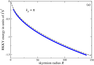
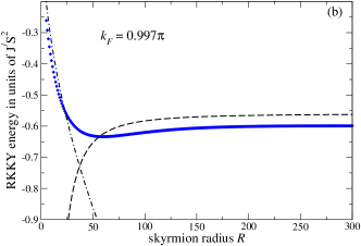
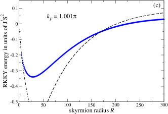
Figure 1: The RKKY contribution to the skyrmion energy as a function of the skyrmion radius $R$ (the lattice constant is set to unity), for a square lattice, at different values of the Fermi wave vector $k_{F}$ around the first “special point”: (a) $k_{F}=\pi$; (b) $k_{F}=0.997\pi$; (c) $k_{F}=1.001\pi$. Symbols denote the numerical results calculated via formula (II.2), and lines correspond to asymptotic expressions (16). The cutoff in sum (II.2) was set to $L=10^{4}$ for $k_{F}=\pi$, and to $L=2000$ for $k_{F}=0.997\pi$ and $k_{F}=1.001\pi$.

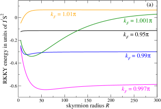
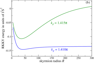
Figure 2: The RKKY contribution to the skyrmion energy as a function of the skyrmion radius $R$ (the lattice constant is set to unity), for a square lattice, at different values of the Fermi wave vector $k_{F}$: (a) evolution of the $R$-dependence when moving away from the special value $k_{F}=\pi$; (b) behavior of the RKKY energy around the second special value $k_{F}=\pi\sqrt{2}$. The cutoff in the sum (II.2) was set to $L=2000$.

III Metallic substrate

For the case of a 2D magnet on top of a metallic substrate, we study the effect of the RKKY interaction using the free electron expression RKKY :

$$f(\bm{\Delta})=\frac{\cos(2k_{F}\Delta)}{(2k_{F}\Delta)^{3}}-\frac{\sin(2k_{F}\Delta)}{(2k_{F}\Delta)^{4}},$$ (12)

where $k_{F}$ is the Fermi wave vector (the radius of the Fermi sphere). For real metals, the situation is more complicated and will be discussed later.

It should be noted that Eq. (12) works fine even for $\Delta\sim 1$ and thus can be taken as an adequate description of both the short- and long-range part of the RKKY exchange.

We will see that the skyrmion stabilization takes place only in narrow regions around some special values of $k_{F}$ which are different in the ferromagnetic and antiferomagnetic cases. For the sake of simplicity, we consider the 2D square lattice.

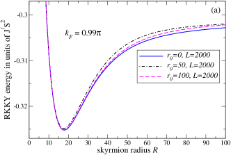
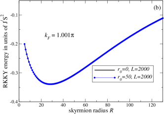
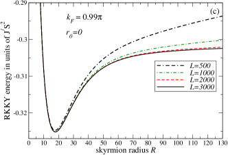
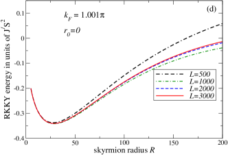
Figure 3: Analysis of errors in the RKKY contribution to the skyrmion energy, introduced by “semi-continuum” approximation and by the finite cutoff $L$: (a,b) results of the “hybrid” calculation using the exact sum in (10) over $|\bm{r}|$ smaller than a certain radius $r_{0}$, and falling back to the continuum approximation in $\bm{r}$ for $|\bm{r}|>r_{0}$, for different values of $r_{0}$ at fixed $L=2000$; (c,d) calculations in “semi-continuum” approximation ($r_{0}=0$) at different values of the cutoff $L$.

III.1 Ferromagnet

To obtain an analytical estimate for the dependence of the energy correction $\Delta E_{\rm RKKY}$ on the skyrmion radius $R$, we will make a few simplifications. First, we drop the second term in (12) as it decays much faster with distance $\Delta$, and we will see that main contribution to the energy comes from $\Delta\sim R\gg 1$. Second, we observe that in (II.2) $\eta_{\bm{\Delta}}=1$ and the lattice sum over $\Delta$ has the same structure as the sum computed by Kamberský et al. Kambersky+99 who studied the effect of the RKKY interaction on the spin wave dispersion. Following Ref. Kambersky+99, , we see that the sum in (II.2) has peculiarities if $2k_{F}$ is close to the length of one of the vectors $\bm{G}$ of the reciprocal lattice, i.e., if $k_{F}$ is close to one of the “special points” $\pi\sqrt{n^{2}+m^{2}}$, where $n$ and $m$ are integers. Those are the same special points around which a strong renormalization of spin wave stiffness occurs Kambersky+99 .

Let us consider the vicinity of the first special point, setting

$$k_{F}=\pi(1-\delta)$$ (13)

with $|\delta|\ll 1$; then the main contribution to the lattice sum in (II.2) comes from the four “cones” around the directions $\bm{\Delta}=(0,\pm 1)$ and $\bm{\Delta}=(\pm 1,0)$. After converting those sums to integrals, one can easily analyze the asymptotic behavior at small and large $R$ (see Appendix A for details). It is convenient to express the results in terms of the quantity

$$w_{\rm FM}=\frac{\pi^{2}(1-\delta)^{3}}{J^{\prime}S^{2}}\Delta E_{\rm RKKY}\simeq-\sqrt{\frac{R}{8}}A(2\pi\delta R)+1,$$ (14)

where the function $A(Q)$ is analyzed in Appendix A and has the following asymptotics:

$$A(Q)\simeq 3.76+16.47\,Q,\quad|Q|\ll 1,$$

$$A(Q)\simeq\begin{cases}\sqrt{2\pi/Q}\Big{(}1+\frac{1}{8Q^{2}}\Big{)},&Q\gg 1\\ \frac{\pi}{2}\sqrt{\pi/|Q|}e^{-2|Q|},&Q\ll-1\end{cases}.$$ (15)

Then for small $R$ one obtains

$$w_{\rm FM}\simeq 1-\sqrt{R}\left(1.33+5.82\cdot(2\pi\delta R)\right),\quad 2\pi\delta R\ll 1,$$ (16a)

while for large radii, $$2\pi\delta R\gg 1$$, the result is

$$w_{\rm FM}\simeq\begin{cases}1-\frac{1}{\sqrt{8\delta}}\left(1+\frac{1}{8(2\pi\delta R)^{2}}\right),&\delta>0,\\ 1-\frac{\pi}{8\sqrt{|\delta|}}e^{-4\pi|\delta|R},&\delta<0\end{cases}.$$ (16b)

One can see that the RKKY correction depends on the skyrmion radius $R$ in a non-monotonic way, with a minimum. At intermediate $1\ll R\ll(2\pi\delta)^{-1}$, the RKKY interaction to the skyrmion is proportional to $-J^{\prime}\sqrt{R}$, which, together with the easy-axis anisotropy contribution (8) that goes roughly as $KR^{2}$, leads to stabilization of the skyrmion radius at some value $R_{0}\propto(J^{\prime}/K)^{2/3}$. A similar picture can be obtained in the vicinity of $k_{F}=\pi\sqrt{2}$ and other “special points”.

Fig. 1 shows the comparison of numerical results obtained by direct calculation of the “semi-continuum” sum (II.2) on a square lattice with the asymptotic expressions (16). One can see that indeed around the special value of the Fermi wave vector $k_{F}=\pi$ the RKKY contribution tends to stabilize the skyrmion, and behaves non-monotonically as a function of the skyrmion radius, in a good agreement with the found asymptotics. However, this stabilization effect deteriorates rapidly away from the special value of $k_{F}$, as one can see in Fig. 2(a): when $k_{F}$ moves away from $\pi$, the minimum moves toward $R=0$ and disappears, and $R$-dependence becomes “flat”. Behavior of the RKKY energy around the second special value $k_{F}=\pi\sqrt{2}$ is qualitatively the same as at the first special point $k_{F}=\pi$, as shown in Fig. 2(b).

Approximating the discrete sum over $\bm{r}$ in Eq. (10) by an integral in the “semi-continuum” approximation of Eq. (II.2) introduces an error which should be at greatest near the skyrmion center, where one has the largest gradients. In order to estimate this error, we have done “hybrid” calculations using the exact sum (10) for $|\bm{r}|$ smaller than some radius $r_{0}$, and falling back to the continuum approximation in $\bm{r}$ for $|\bm{r}|>r_{0}$ (see Eq. (B) in Appendix B); thus, $r_{0}=0$ is equivalent to “semi-continuum” approximation of Eq. (II.2), and $r_{0}\to\infty$ amounts to using Eq.  (10). Calculations for several values of $r_{0}$ are shown in Fig. 3(a,b); one can see that the semi-continuum approximation works very well.

Another source of error is our use of a finite cutoff $|\bm{\Delta}|<L$ in the sum (II.2). Fig. 3(c,d) presents results of calculations for several values of $L$ which show that for skyrmion radii $R<300$ the convergence is already reached at $L=2000$.

Further, we have studied how the skyrmion stabilization might be affected by a finite spin-flip length $\ell_{sf}$ (the average length an electron travels in metal before its spin gets flipped). At room temperature, in pure metals $\ell_{sf}$ ranges from tens to several hundreds of nanometers, but it is strongly dependent on temperature and is affected by the presence of interfaces BassPratt07 . One can expect that the RKKY interaction is exponentially suppressed at distances larger than $\ell_{sf}$. We have modeled this effect by simply introducing the factor $\exp(-\Delta/\ell_{sf})$ into the RKKY power-law (12). The results of such modification are shown in Fig. 4. One can see that decreasing $\ell_{sf}$ leads to a rapid “flattening” of the RKKY energy in the region of large $R\gtrsim\ell_{sf}$, but leaves the initial square-root behavior intact. Thus, even for relatively short $\ell_{sf}$ the sum of the RKKY energy and the anisotropy contribution (8) still has a minimum at some value of $R$ proportional to $(J^{\prime}/K)^{2/3}$, so the stabilization effect is preserved.

III.2 Antiferromagnet

In the antiferromagnetic case, the procedure is very similar to that considered above. We again start from Eq.  (II.2) with $f(\bm{\Delta})$ given by the first term of Eq. (12), but now we have the oscillating factor $\eta_{\bm{\Delta}}=(-1)^{\Delta_{x}+\Delta_{y}}$, which changes the “special points” in $k_{F}$ around which the skyrmion stabilization is possible: now $2k_{F}$ should be close to the length of the vector $\bm{G}+(\pi,\pi)$, where $\bm{G}=2\pi(n_{1},n_{2})$ is an arbitrary reciprocal lattice vector. Thus the first “special point” is $k_{F}=\pi/\sqrt{2}$. As shown in Appendix A, one can obtain the analytical estimate expressing the RKKY contribution to skyrmion energy via the same function $A(Q)$:

$$w_{\rm AFM}\simeq-\frac{\sqrt{R}}{2^{7/4}}A(Q=\pi\sqrt{2}\delta R)+1,$$ (17)

where $w_{\rm AFM}$ is defined in full analogy to Eq. (14). Thus, for the AFM case one can expect qualitatively the same behavior of the RKKY energy as disussed above for the ferromagnet. Numerical results confirm this prediction, as shown in Fig. 5.

III.3 Self-consistency conditions

As mentioned before, our calculations of the skyrmion energy can be viewed as a variational energy estimate obtained by the first-order perturbation theory, with the unperturbed Hamiltonian describing the isotropic Heisenberg magnet, and the two perturbations being the RKKY exchange (proportional to $J^{\prime}$) and the easy-axis anisotropy (proportional to $K$). We look at the sector with the topological charge $\nu=1$, where the unperturbed solution is given by the BP soliton, and this solution is used as a basis to calculate contributions to the skyrmion energy from the two perturbations.

Here, however, there is a subtle point: although, as we have shown, the RKKY contribution is not singular in $J^{\prime}$, it is well known that the contribution from the easy-axis anisotropy is non-analytical in $K$ (see Eq. (8)). This is due to the fact that the anisotropy changes the power-law decay of the BP solution to the exponential one at distances $r>\ell_{0}\sim(J/K)^{1/2}$, and the BP solution modified by the anisotropy is well described, e.g., by the following ansatz proposed in Ref. VoronovIvanovKosevich, )

$$\tan(\theta/2)=\frac{2}{(\nu-1)!}\left(\frac{R}{2\ell_{0}}\right)^{|\nu|}K_{\nu}\left(\frac{r}{\ell_{0}}\right),$$

where $K_{\nu}(z)$ is the modified Bessel function of the second kind (the Macdonald function). The above ansatz in principle could be used for a direct computation of the double sum (7), but the integration over $\bm{r}$ could not be performed analytically. However, one can use the following argument: the effect of the finite anisotropy on the RKKY contribution is roughly equivalent to introducing cutoffs of about $\ell_{0}$ both for $r$ and $\Delta$ in the sum defined by Eq. (7). One can reasonably assume that those cutoffs will not qualitatively affect our results for skyrmion radii much smaller than the cutoff, $R\ll\ell_{0}$. As we have shown above, for $k_{F}$ sufficiently close to one of the ”special points” the RKKY energy gain is proportional to $R^{1/2}$ for $R\ll 1/(2\pi\delta)$, and then the skyrmion energy minimum is reached at $R=R_{0}\sim(J^{\prime}/K)^{2/3}$. Thus, our results should remain valid as long as $R_{0}$ is much smaller than both the cutoff $\ell_{0}$ and $1/(2\pi\delta)$, which leads to the following self-consistency conditions:

$$J^{\prime}\ll(J^{3}K)^{1/4},\quad J^{\prime}\ll K(2\pi\delta)^{-3/2}.$$

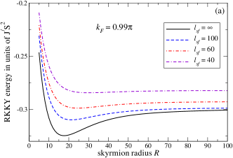
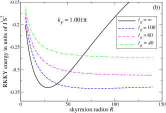
Figure 4: Influence of the finite spin-flip length $\ell_{sf}$ on the RKKY contribution to the skyrmion energy: (a) $k_{F}=0.99\pi$; (b) $k_{F}=1.001\pi$. The cutoff in the sum over $\bm{\Delta}$ in (II.2) was set to $L=2000$.

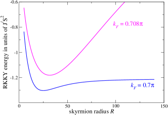
Figure 5: The RKKY contribution to the skyrmion energy for an antiferromagnet on a square lattice, around the first special point $k_{F}=\pi/\sqrt{2}$. The cutoff in the sum over $\bm{\Delta}$ is $L=2000$.

IV Graphene substrate

The RKKY interaction in graphene is in many respects considerably different from such in a normal two-dimensional metal (see, e.g., Ref. PowerFerreira13, for a review). RKKY interaction between magnetic adatoms at a graphene monolayer strongly depends on how are the adatoms placed with respect to the carbons of the graphene. The geometry of the lowest energy configuration depends on the adatoms concentration: for instance, while single Co atoms are adsorbed on graphene “hollow sites” (centers of hexagons) Donati+13 , graphene grown on Co(0001) substrate exhibits 3-fold symmetry consistent with top-fcc or top-hcp configurations Kaul+12 ; Usachov+15 where Co atoms of the proximate layer sit on top of the carbons belonging to only one sublattice. This might be caused by the van der Waals interaction contributing significantly to the interaction between the substrate (or adatoms) and graphene Stradi+11 ; Kaul+12 .

We focus on a simplified model of two lattice-matched monolayers (graphene and magnetic). We will restrict ourselves to the case of ferromagnetic Heisenberg exchange between magnetic atoms, and we will consider two possible geometries: (a) magnetic atoms sitting on top of each carbon of the graphene layer, forming a hexagonal lattice, and (b) magnetic atoms sitting at the centers of hexagons (“hollow sites”), forming a triangular lattice.

IV.1 “On-top” configuration

In the case of magnetic atoms sitting on top of the carbon atoms of undoped (half-filled) graphene, particle-hole symmetry leads to ferromagnetic interaction between spins on the same graphene sublattice and antiferromagnetic interaction of spins on different sublattices Saremi07 ; Brey+07 ; Black-Schaffer10 . In a simple tight-binding model of graphene with two “impurity” spins sitting on top of carbons and coupled to the itinerant electrons of graphene via the Heisenberg exchange $\tilde{J}$, the characteristic magnitude of the RKKY exchange is Kogan11 $J^{\prime}=a_{0}\tilde{J}^{2}/(256\hbar v_{F})$, where $v_{F}$ is the Fermi velocity and $a_{0}$ is the carbon-carbon distance which is hereafter set to unity. The RKKY exchange $J^{\prime}f_{AA,AB}(\bm{\Delta})$ between two impurity spins sitting on the same sublattice (AA) or different sublattices (AB), where $\bm{\Delta}$ is the vector connecting the two magnetic atoms, is determined by the following expresions SherafatiSatpathy11 ; Kogan11 :

$$f_{AA}(\bm{\Delta}) = -\frac{1+\cos[(\bm{K}-\bm{K^{\prime}})\cdot\bm{\Delta}]}{\Delta^{3}},$$ (18)

$$f_{AB}(\bm{\Delta}) = 3\frac{1+\cos[(\bm{K}-\bm{K^{\prime}})\cdot\bm{\Delta}+\pi-2\theta_{\Delta}]}{\Delta^{3}},$$ (19)

where $\bm{K}$ and $\bm{K^{\prime}}$ are a pair of adjacent Dirac points, and $\theta_{\Delta}$ is the angle between vectors $\bm{\Delta}$ and $\bm{K^{\prime}}-\bm{K}$ (see Fig. 6). We choose $\bm{K},\bm{K^{\prime}}=\frac{2\pi}{3}(\mp\frac{1}{\sqrt{3}},1)$, then Eqs. (18), (19) are valid in the $60^{\circ}$-sector $\theta_{\Delta}\in[-\frac{\pi}{6},\frac{\pi}{6}]$; in the rest of the plane the pattern of $f_{AA,AB}(\bm{\Delta})$ repeats according to the symmetry. Two important points are worth noting: (i) although the RKKY interaction (18), (19) is oscillating, both $f_{AA}$ and $f_{AB}$ are not sign-changing; (ii) the magnitudes of intra-sublattice and inter-sublattice interactions are different.

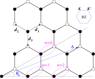
Figure 6: Schematic view of the graphene layer showing the notation used in Eqs. (18), (19). Two different sublattices are shown with full and open circles. The orientation of the Brillouin zone and the chosen adjacent pair of Dirac points $\bm{K}$, $\bm{K^{\prime}}$ are indicated, as well as the three nearest-neighbor vectors $\bm{d}_{1,2,3}$. Three ellipses show the cluster of sites used when calculating the average (20).

To analyze the RKKY contribution to skyrmion energy, we again use the “semi-continuum” approximation (II.2), where now the sum over $\bm{\Delta}$ has to be broken into AA and AB parts, and the area per lattice site is $\mathcal{A}_{0}=3\sqrt{3}/4$ (in units of $a_{0}^{2}$). To deal with oscillating contribution from the cosines in (18), (19), it is convenient to parametrize the distance vector as $\bm{\Delta}=m(\bm{d}_{1}-\bm{d}_{2})+l\bm{d}_{1}$, where $m$ and $l$ are non-negative integers ($l=1+3s$ for AB interaction and $l=3s$ for the AA part, where $s=0,1,2,\ldots$), see Fig. 6. It is easy to see that the pattern of $f_{AA}$ and $f_{AB}$ exhibits threefold periodicity in $m$ as shown in Table 1. Further, $g(\Delta/R)$ in (II.2) is a smooth function, and for $R\gg 1$ it changes only slightly when $\Delta$ changes by something of the order of unity. Then, when computing the sum over $\bm{\Delta}$, we can separate it into clusters of six sites with approximately the same $\Delta$, as shown by three ellipses in Fig.  6. The value of $f(\bm{\Delta})$, averaged over such a six-site cluster, is

$$\bar{f}(\bm{\Delta})=\frac{1}{6}\sum_{j=0,1,2}\Big{(}f_{AA}^{m=j+3k}+f_{AB}^{m=j+3k}\Big{)}\simeq\frac{1}{\Delta^{3}},$$ (20)

where we have just neglected differences in $m$ and $l$ between the sites of the cluster. As one can see, this procedure is roughly equivalent to neglecting the oscillating contribution of the cosines in (18), (19). Because of unequal magnitudes of intra-sublattice and inter-sublattice interactions, the averaged RKKY interaction (20) has positive (AFM) sign, which is crucial for the skyrmion stabilization effect.

	$m=3k$	$m=1+3k$	$m=2+3k$
$f_{AA}$	$-\frac{2}{\Delta^{3}}$	$-\frac{1}{2\Delta^{3}}$	$-\frac{1}{2\Delta^{3}}$
$f_{AB}$	$\frac{6}{\Delta^{3}}-\frac{9m^{2}}{2\Delta^{5}}$	$\frac{3l^{2}}{2\Delta^{5}}$	$\frac{3}{\Delta^{3}}+\frac{9m^{2}-3l^{2}}{2\Delta^{5}}$

Table 1: Pattern of the RKKY interactions (18), (19); $m$, $l$, and $k$ are integer numbers, $\bm{\Delta}=(m+l)\bm{d}_{1}-m\bm{d}_{2}$, $\Delta^{2}=l^{2}+3m(m+l)$.

After substituting the averaged RKKY amplitude (20) into (II.2), we can pass to continuum, converting the sum over $\bm{\Delta}$ into an integral; this yields the following asymptotic behavior of the RKKY contribution $\Delta E_{\text{RKKY}}$ to skyrmion energy:

$$\frac{\Delta E_{\text{RKKY}}}{J^{\prime}S^{2}} \simeq -\frac{2\pi^{2}R}{\mathcal{A}_{0}^{2}}\int_{1/R}^{\infty}\frac{dx}{x}g(x)$$ (21)

$$= -\frac{16\pi^{4}}{27}R+\frac{32\pi^{2}}{27}+O(R^{-2}).$$

Thus, RKKY interaction via single-layer graphene leads to the contribution into the skyrmion energy proportional to $-CJ^{\prime}R$, with a strong enhancement factor $C\sim 60$. Together with the easy-axis anisotropy contribution (8) that is roughly proportional to $KR^{2}$, this leads to skyrmion stabilization at radius value $R_{0}\propto CJ^{\prime}/K$.

Fig. 7(a) shows the comparison of numerical results obtained by direct calculation of the lattice sum (10) with several different cutoffs, and by using the “semi-continuum” sum (II.2), with the asymptotic expression (21).

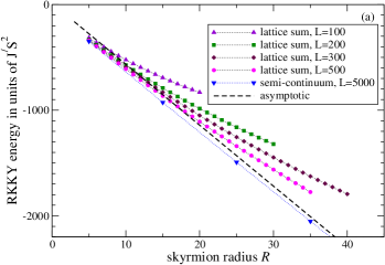
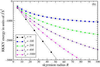
Figure 7: Numerical results for the RKKY contribution to skyrmion energy, in a 2D ferromagnet at single layer graphene in “on-top” geometry: (a) results obtained by direct calculation of the lattice sum (10) with different cutoffs (the same cutoff $L$ is used for $|\bm{\Delta}|$ and $|\bm{r}|$) are shown in comparison to those obtained in semi-continuum approximation (II.2), the dashed line corresponds to the asymptotic formula (21); (b) the effect of a finite spin-flip length $\ell_{sf}$ (calculated in the semi-continuum approximation).

Within the same approximation, it is easy to estimate the effect of a finite spin-flip length as well. Introducing the exponentially decaying factor $\exp(-\Delta/\ell_{sf})$ into (18), (19) as we have done for the metallic substrate, we obtain

$$\frac{\Delta E_{\text{RKKY}}}{J^{\prime}S^{2}}\simeq-\frac{2\pi^{2}R}{\mathcal{A}_{0}^{2}}\int_{1/R}^{\infty}\frac{dx}{x}g(x)\exp(-xR/\ell_{sf}),$$ (22)

which falls back to (21) for $R\ll\ell_{sf}$, and goes to a constant, ${\Delta E_{\text{RKKY}}}/{J^{\prime}S^{2}}\simeq-\frac{32\pi^{2}R}{27}\ell_{sf}$ for $R\gg\ell_{sf}$. The influence of a finite spin-flip length is illustrated in Fig. 7(b). The typical value of spin-flip length in undoped graphene Dlubak+12 ; Yan+16 is rather large, $\ell_{sf}\sim 100$ $\mu$m which corresponds to about $10^{5}a$, so this effect is likely to be negligible in practice.

IV.2 “Hollow sites” configuration

For magnetic atoms placed at the “hollow sites” of graphene lattice (i.e., at centers of hexagons), the RKKY interaction takes a very simple form which is radially symmetric, non-oscillating, and antiferromagnetic Saremi07 ; Black-Schaffer10 ; SherafatiSatpathy11 :

$$f(\bm{\Delta})=36J^{\prime}/\Delta^{3}.$$ (23)

Calculation of the RKKY contribution to skyrmion energy in the “semi-continuum” approximation (II.2) is thus essentially reproducing the steps done above in the derivation of Eq. (21); there is just an extra overall factor of $36$, and the area per magnetic atom is doubled, $\mathcal{A}_{0}=3\sqrt{3}/2$. As a result, one obtains the following asymptotic expression:

$$\frac{\Delta E_{\text{RKKY}}}{J^{\prime}S^{2}}\simeq-\frac{16\pi^{4}}{3}R+\frac{32\pi^{2}}{3}+O(R^{-2}).$$ (24)

Note that the enhancement factor (the number in front of $R$ in the above formula) is in this case quite large, $\sim 500$. In other respect, the effect of the RKKY interaction is in this case the same as for the “on-top” configuration.

Comparing the above results with those of Sect. III, one can notice that the energy gain due to the RKKY interaction is considerably larger for a graphene substrate than for a normal metal. Indeed, according to the asymptotic formula (16b), for a metallic substrate the maximal energy gain in units of $J^{\prime}S^{2}$ is limited by some value of the order of unity, as illustrated by Fig. 1. At the same time, for a graphene substrate the RKKY energy gain is not capped and continues to increase linearly with the skyrmion size $R$, as follows from the asymptotic formula (21) and seen in Fig. 7. The reason is, for a normal metal the RKKY interaction oscillates in such a way that its net effect integrates almost to zero, and the total energy gain is modest. For graphene, the situation is different (see Eqs. (18), (19)): (i) either within the sublattice or between sublattices, RKKY oscillations occur on top of a finite value, in such a way that the sign of the RKKY exchange stays constant; (ii) the magnitude of the intersublattice RKKY exchange is three times larger than that of the intra-sublattice one. As a result, the net effect of the RKKY exchange in graphene on the skyrmion energy is much larger than in the case of a normal metal.

V Discussion and Summary

We have demonstrated the stabilizing effect of the RKKY interaction on an isolated magnetic skyrmion in a 2D magnet, in two scenarios involving the RKKY interaction via a normal metallic substrate or via single-layer graphene. For both scenarios, we have used simple expressions for the RKKY exchange obtained in models of non-interacting itinerant electrons (free electrons with a spherical Fermi surface in the case of a normal metal, and the tight-binding model for graphene). In both cases, we have found that the RKKY interaction yields a negative contribution to the skyrmion energy of the type $-(R/a)^{\alpha}$, $\alpha\leq 1$, where $R$ is the skyrmion radius. This contribution counteracts the skyrmion tendency to collapse (caused by the contribution from the easy-axis anisotropy proportional to $(R/a)^{2}$) and provides a novel mechanism of the skyrmion stabilization.

For the RKKY coupling via a metallic substrate, our main conclusion is that the skyrmion stabilization is possible under certain conditions on the Fermi wave vector $k_{F}$ (namely, in the case of a ferromagnet $2k_{F}$ should be close to the length of one of the vectors $\bm{G}$ of the reciprocal lattice, and for an antiferromagnet $2k_{F}$ should be close to the length of the vector $\bm{G}+(\pi,\pi)$). The special values of $k_{F}$ are exactly those where pecularities of the spin wave stiffness occur Kambersky+99 , leading to modifications of the long-wavelength spin wave dispersion that is non-analytic in the wave vector. We have shown that if the above conditions on $k_{F}$ are satisfied, the contribution of the RKKY interaction to the skyrmion energy is proportional to $-(R/a)^{1/2}$, non-analytic in $R$. Such non-analytic contributions, either to the magnon spectrum or to the skyrmion energy, cannot be described by a finite number of exchange interactions beyond the nearest neighbors, so the resulting physics is very different from that studied by Abanov and Pokrovsky AbanovPokrovsky98 .

One may wonder whether the above-mentioned conditions on $k_{F}$ can be realized in practice. Extending the simple RKKY model to take into account real shapes of Fermi surfacesRoth+66 leads to the RKKY oscillations containing, instead of one wave vector $2k_{F}$, several wave vectors $2k_{v}$ corresponding to the diameters connecting so-called caliper points of the Fermi surface. As shown in Ref. Kambersky+99, , for the ideal epitaxial monolayer of magnetic atoms on a (001) plane of a fcc metal with fcc lattice (Ag, Cu, Au), one has pairs of such caliper points satisfying $2k_{v}=(1\pm\delta)|\bm{G}|$ with $\delta\approx 0.04\div 0.06$. Though being close to the “resonance”, this might be still too far from it for the stabilization, as seen from Fig. 2. Further fine-tuning of the shape of the Fermi surface might be achieved by diluting the metallic layer SatoToth62 ; TempletonColeridge75 , or by applying external pressure Lazarev+65 ; Egorov+84 ; Gaidukov+84 (possibly also via the interface-induced strain); the external pressure can alter not only the shape, but even the topology of the Fermi surface Lazarev+65 .

For the RKKY coupling via a single-layer graphene, we have shown that at least in two considered geometries (magnetic atoms on top of the carbons on both sublattices, and magnetic atoms at hollow sites) the stabilization is naturally achieved without any fine-tuning (only the ferromagnetic case has been considered). The crucial point, leading to that effect, is the unequal magnitude of intra-sublattice (ferromagnetic) and inter-sublattice (antiferromagnetic) RKKY interaction in graphene: the inter-sublattice coupling is three times stronger, which, on the net, leads to a negative (stabilizing) contribution to the skyrmion energy proportional to the skyrmion radius $R$. One may speculate, that in the case of a lattice mismatch between the magnetic layer and graphene, the average effect will be the same, leading to skyrmion stabilization. Actually, the only geometry unfavorable for the skyrmion stabilization is that with magnetic atoms on top of the only one carbon sublattice: then the RKKY contribution to the energy is positive and does not prevent the skyrmion collapse.

Experimentally, one of the problems of dealing with graphene/ferromagnetic interfaces is the transfer of outer electrons of magnetic adatoms to the graphene layer, which might lead to doping or to the presence of weakly localized states in graphene, modifying the RKKY interaction DedkovFonin10 ; DedkovVoloshina15 . Doping the graphene layer (or applying a gate voltage) introduces additional oscillations with the finite Fermi wave vector $2k_{F}$ in the RKKY interaction SherafatiSatpathy11a , which opens an interesting possibility of tuning the $k_{F}$ to one of the singular points.

It should be emphasized that the approximate analysis used in the present work can be viewed as a variational energy estimate obtained within the first-order perturbation theory, with the unperturbed Hamiltonian describing the isotropic Heisenberg magnet, and the two perturbations being the RKKY exchange and the easy-axis anisotropy. Although one can assess the stability of a skyrmion against collapse in this way, it does not constitute a full proof of stability. To analyze such a stability, one would need to find the full set of magnon eigenmodes on top of the soliton background. While this problem can be solved for the “standard” model with the local exchange interaction Sheka+01 , the eigenvalue problem in presence of long-range exchange interactions is much more involved and remains, to the best of our knowledge, unexplored. Nevertheless, one can make the following argument: the eigenmode frequencies $\omega_{n,m}$ are characterized by the azimuthal number $m$ and the principal number $n$. An instability is reflected in the appearance of negative $\omega_{n,m}^{2}$ for some values of $m$. The radial stability is connected to $m=0$, and is fully determined by the energy $W(R)$ studied in the present work, because $\omega_{n,m=0}^{2}\propto d^{2}W(R)/dR^{2}$. Thus, a minimum in $W(R)$, as found in this work, ensures that the soliton is stable against a radial perturbation, i.e., against the collapse. Note that the only terms contributing to the $R$-dependence of the energy are those breaking the scale invariance, i.e., the RKKY coupling and anisotropy (but not the nearest-neighbor exchange). The $m=1$ mode describes a shift of the skyrmion as a whole and thus does not correspond to any instability. A negative $\omega_{n,m=2}^{2}$ would correspond to the elliptical instability, which is, e.g., known for magnetic bubbles in presence of the dipole-dipole interaction. However, in the absence of other interactions the stiffness coefficients $\omega_{n,m}^{2}$ for $m\geq 2$ are all positiveSheka+01 and their scale is set by the nearest-neighbor exchange $J$. Thus, one can expect that no instabilities arise if the RKKY exchange and anisotropy are small compared to the nearest-neighbor exchange, $J^{\prime},K\ll J$ (as assumed throughout the present paper). We hope that our analysis will stimulate the corresponding numerical work which will deliver the true skyrmion solutions in presence of the RKKY exchange and the easy-axis anisotropy.

Finally, we would like to mention that we have considered only the effect of 2nd-order (RKKY) exchange between spins of a magnetic insulator, interacting via the metallic substrate. In the case of itinerant magnets, higher-order (multispin) interactions might become important Ozawa+17prl ; *Hayami+17prb, but this is beyond the scope of the present work.

Appendix A Asymptotic behavior of the RKKY energy correction

In this Appendix we provide details of the analysis leading to the asymptotic expressions (III.1). In all calculations, we assume that the skyrmion radius is always much larger than the lattice constant, $R\gg 1$.

Ferromagnetic case.–

We start from Eq.  (II.2) with $\eta_{\bm{\Delta}}=1$, $f(\bm{\Delta})$ given by the first term of Eq. (12), and $k_{F}=\pi(1-\delta)$, $|\delta|\ll 1$ and notice that the main contribution to the lattice sum in (II.2) comes from the four equivalent “cones” around the directions $\bm{\Delta}=(0,\pm 1)$, $\bm{\Delta}=(\pm 1,0)$. Following the procedure of Ref. Kambersky+99, , a contribution of one “cone” can be approximately calculated as follows: put $\bm{\Delta}=(n,m)$, where $n$ and $m$ are integers, with $|n|\ll m$, then inside the cosine $\cos(2k_{F}\Delta)$ one can expand $\Delta$ in $n$, $\Delta\simeq m+n^{2}/(2m)$, and in the rest of the expression one can set $\Delta\simeq m$, so we have

$$w_{\rm FM}\simeq-\frac{R}{2}\sum_{m=1}^{\infty}\frac{g(\frac{m}{R})}{m^{2}}\sum_{n=-m+1}^{m}\Big{\{}\cos\frac{\pi n^{2}}{m}\cos(2\pi\delta m)$$

$$\qquad+\sin\frac{\pi n^{2}}{m}\sin(2\pi\delta m)\Big{\}},$$ (25)

where $g(x)$ is given by (II.2). Using the fact that

$$\sum_{n=-m+1}^{m}\cos\frac{\pi n^{2}}{m} = \begin{cases}0,&m=\text{odd}\\ \sqrt{2m},&m=\text{even}\end{cases},$$ (26)

$$= \sum_{n=-m+1}^{m}\sin\frac{\pi n^{2}}{m},$$

we rewrite the RKKY correction as

$$w_{\rm FM}\simeq-\frac{R}{4}\sum_{l=1}^{\infty}\frac{g(2l/R)}{l^{3/2}}\Big{\{}\cos(4\pi\delta l)+\sin(4\pi\delta l)\Big{\}}.$$ (27)

Assuming that $R\gg 1$ and $\delta\ll 1$, and passing from the discrete sum to the continuum, we finally obtain

$$w_{\rm FM}\simeq-\sqrt{\frac{R}{8}}A(2\pi\delta R)+1,$$ (28)

where

$$A(Q)=\Re I(Q)+\Im I(Q),\quad I(Q)=\int_{0}^{\infty}dx\,\frac{g(x)}{x^{3/2}}e^{iQx},$$ (29)

and the second term in (28) is the correction coming from the fact that actually the lower integration limit in $I(Q)$ should be not zero but $2/R$. The integral $I(Q)$ above can be easily analyzed: integrating $p(z)=\frac{g(z)}{z^{3/2}}e^{iQz}$ along the contour shown in Fig. 8 should obviously give zero. Assuming $Q>0$, and sending the contour radius to infinity, one can see that integrals over subcontours behave as

$$\int_{C_{1}}p(z)dz\to I(Q),\quad\int_{C_{2}}p(z)dz\to 0,$$

$$\int_{C_{3}}p(z)dz\to-\pi\sqrt{2}(1-i)F(Q)+\frac{1+i}{\sqrt{2}}P(Q),$$

$$\int_{C_{4}}p(z)dz\to-(1+i)S(Q),$$ (30)

where we have used the following notation:

$$F(Q) = \int_{2}^{\infty}dy\frac{e^{-Qy}}{y^{3/2}\sqrt{y^{2}-4}},$$

$$S(Q) = \int_{0}^{\pi/2}d\varphi\frac{\varphi}{\sin^{3/2}\varphi}e^{-2Q\sin\varphi},$$ (31)

$$P(Q) = \int_{2}^{\infty}dy\frac{e^{-Qy}}{y^{3/2}\sqrt{y^{2}-4}}\ln\Big{[}1-2y^{2}+\frac{y^{4}}{2}$$

$$+ y(\frac{y^{2}}{2}-1)\sqrt{y^{2}-4}\Big{]}.$$

Thus, for $Q>0$, real and imaginary parts of $I(Q)$ are expressed via the above three integrals as follows:

$$\Re I(Q) = \pi\sqrt{2}F(Q)-\frac{1}{\sqrt{2}}P(Q)+S(Q),$$

$$\Im I(Q) = -\pi\sqrt{2}F(Q)-\frac{1}{\sqrt{2}}P(Q)+S(Q).$$ (32)

To obtain $I(Q)$ for negative $Q$, one can notice that $\Re I(Q)$ is even in $Q$, while $\Im I(Q)$ is odd. The combination $A(Q)=\Re I(Q)+\Im I(Q)$ entering the energy correction (28) is thus expressed as follows:

$$A(Q)=\begin{cases}2S(Q)-\sqrt{2}P(Q),&Q>0\\ 2\pi\sqrt{2}F(|Q|),&Q<0\end{cases}.$$ (33)

Figure 8: The integration contour and subcontours used in (A). Bold lines denote cuts.

Asymptotic behavior of the integrals $F$, $S$, and $P$ at small and large positive $Q$ can be obtained in a standard way, here we just list the results:

$$F(Q)\simeq\begin{cases}0.42-1.85Q,&Q\ll 1\\ \sqrt{\frac{\pi}{32Q}}e^{-2Q},&Q\gg 1\end{cases},$$ (34)

$$S(Q)\simeq\begin{cases}2.90-2.89Q,&Q\ll 1\\ \sqrt{\frac{\pi}{2Q}}\Big{(}1+\frac{1}{8Q^{2}}\Big{)},&Q\gg 1\end{cases},$$ (35)

$$P(Q)\simeq\begin{cases}1.44-15.73Q,&Q\ll 1\\ \frac{1}{\sqrt{2}Q}e^{-2Q},&Q\gg 1\end{cases}.$$ (36)

After substituting all those expressions into (33), one obtains the asymptotics given by (III.1) and resulting in the expressions (16).

Antiferromagnetic case.–

Setting $k_{F}$ in the vicinity of the first “special point”, $k_{F}=\frac{\pi}{\sqrt{2}}(1-\delta)$, $|\delta|\ll 1$, one can see that the main contribution to the lattice sum in (II.2) comes from the four equivalent “cones” around the directions $\bm{\Delta}=(\pm 1,\pm 1)$, $\bm{\Delta}=(\pm 1,\mp 1)$. The contribution of one “cone” can be approximately calculated as follows: put $\bm{\Delta}=(s+m,s-m)$, where $s$ and $m$ can be either both integer, or both half-integer, with $|m|\ll s$, then $\eta_{\bm{\Delta}}=(-1)^{2s}$, inside the cosine $\cos(2k_{F}\Delta)$ one can expand $\Delta$ in $m$, $\Delta\simeq s\sqrt{2}\big{[}1+m^{2}/(2s)\big{]}$, and in the rest of the expression one can set $\Delta\simeq s\sqrt{2}$. This yields

$$w_{\rm AFM}\simeq-\frac{R}{2^{5/2}}\sum_{s=\frac{1}{2},1,\frac{3}{2},\ldots}\frac{g\left(\frac{s\sqrt{2}}{R}\right)}{s^{2}}$$ (37)

$$\quad\sum_{m=-s+1}^{s}\Big{\{}\cos\frac{\pi m^{2}}{s}\cos(2\pi\delta s)+\sin\frac{\pi m^{2}}{s}\sin(2\pi\delta s)\Big{\}}.$$

Sums over $m$ can be readily performed: for integer $s$ they are given by Eq. (26), and for half-integer $s=l+\frac{1}{2}$ one has

$$\sum_{m=-l+\frac{1}{2}}^{l+\frac{1}{2}}\cos\frac{\pi m^{2}}{l+\frac{1}{2}}=\begin{cases}\sqrt{2l+1},&l=\text{odd}\\ 0,&l=\text{even}\end{cases},$$ (38)

$$\sum_{m=-l+\frac{1}{2}}^{l+\frac{1}{2}}\sin\frac{\pi m^{2}}{l+\frac{1}{2}}=\begin{cases}\sqrt{2l+1},&l=\text{even}\\ 0,&l=\text{odd}\end{cases}.$$ (39)

Passing in the remaining sum over $s$ to the continuum, one can approximately express the RKKY energy correction in terms of the same function (29) introduced above in the ferromagnetic case:

$$w_{\rm AFM}\simeq-\frac{\sqrt{R}}{2^{7/4}}A(Q=\pi\sqrt{2}\delta R)+1,$$ (40)

where the origin of the second term is the same as in Eq. (28), namely, the correction connected with the nonzero lower integration limit when passing to the continuum. Thus, the behavior of the energy correction on the skyrmion radius $R$ for an antiferromagnet is qualitatively similar to that for a ferromagnet. The only important difference is the change of the condition for the Fermi wave vector.

Appendix B “Hybrid” formula for the lattice sum

Numerical computation of the fourfold lattice sum (10) over $\bm{r}$, $\bm{\Delta}$can be a resource-intensive task for large lattices. “Semi-continuum” formula (II.2), which converts the sum over $\bm{r}$ into an integral, simplifies this task considerably, but introduces an uncontrollable approximation. To estimate the errors of this approximation, one can undertake a “hybrid” approach, using the sum (10) for $|\bm{r}|$ smaller than some radius $r_{0}$, and passing to the continuum in $\bm{r}$ for $|\bm{r}|>r_{0}$. The corresponding expression is easily derived and has the following form:

$$\frac{\Delta E_{\rm RKKY}}{J^{\prime}S^{2}} = -R^{2}\sum_{\bm{\Delta}}\eta_{\bm{\Delta}}\Delta^{2}f(\bm{\Delta})\left\{\sum_{|\bm{r}|<r_{0}}\frac{(r^{2}+R^{2}+\Delta^{2})}{(r^{2}+R^{2})[(r^{2}+R^{2}+\Delta^{2})^{2}-4(\bm{r}\cdot\bm{\Delta})^{2}]}+\frac{\pi}{R^{2}}h\left(\frac{\Delta}{R},\frac{r_{0}}{R}\right)\right\},$$

$$h(x,y) = \frac{1}{x\sqrt{4+x^{2}}}\ln\Big{[}\frac{x(3+x^{2}-y^{2})+\sqrt{4+x^{2}}\sqrt{(x^{2}+1)^{2}+y^{2}(2-2x^{2}+y^{2})}}{(1+y^{2})(\sqrt{4+x^{2}}-x)}\Big{]}$$ (41)

References

- (1) A. Fert, N. Reyren, and V. Cros, Nat. Rev. Mater. 2, 17031 (2017).
- (2) A. Fert, V. Cros, and J. Sampaio, Nature Nanotechnol. 8, 152 (2013).
- (3) N. Nagaosa and Y. Tokura, Nature Nanotechnol. 8, 899 (2013).
- (4) N. Romming, C. Hanneken, M. Menzel, J. E. Bickel, B. Wolter, K. von Bergmann, A. Kubetzka, and R. Wiesendanger, Science 341, 636 (2013).
- (5) W. Koshibae, Y. Kaneko, J. Iwasaki, M. Kawasaki, Y. Tokura, and N. Nagaosa, Jpn. J. Appl. Phys. 54, 053001 (2015).
- (6) F. Jonietz, , S. Mühlbauer, C. Pfleiderer, A. Neubauer, W. Münzer, A. Bauer, T. Adams, R. Georgii, P. Böni, R. A. Duine, K. Everschor, M. Garst, and A. Rosch, Science 330, 1648 (2010).
- (7) X. Z. Yu, N. Kanazawa, W.Z. Zhang, T. Nagai, T. Hara, K. Kimoto, Y. Matsui, Y. Onose, and Y. Tokura, Nature Commun. 3, 988 (2012).
- (8) J. Iwasaki, M. Mochizuki, and N. Nagaosa, Nature Commun. 4, 1463 (2013).
- (9) N. S. Kiselev, A. N. Bogdanov, R. Schäfer, and U. K. Rößler, J. Phys. D 44, 392001 (2011).
- (10) M. Schott, A. Bernand-Mantel, L. Ranno, S. Pizzini, J. Vogel, H. Béa, C. Baraduc, S. Auffret, G. Gaudin, and D. Givord, Nano Letters 17, 3006 (2017).
- (11) R. Hobart, Proc. Phys. Soc. 82, 201 (1963).
- (12) G. M. Derrick, J. Math. Phys. 5, 1252 (1964).
- (13) E. G. Galkina, B. A. Ivanov and V. A. Stephanovich, J. Magn. Magn. Mater. 118, 373 (1993).
- (14) T. H. R. Skyrm, Proc. R. Soc. A, 260, 127 (1961).
- (15) T. H. R. Skyrm, Nucl. Physics 31, 556 (1962).
- (16) A. Hubert and R. Schäfer, Magnetic Domains (Springer, Berlin, 1998).
- (17) A. A. Belavin and A. M. Polyakov, JETP Lett. 22, 245 (1975)
- (18) F. Waldner, J. Magn. Magn. Mater. 54, 873 (1986).
- (19) B. A. Ivanov and V. A. Stefanovich, Zh. Eksp. Teor. Fiz. 91, 638 (1986) [Sov. Phys. JETP 64, 376 (1986)].
- (20) B. A. Ivanov, V. A. Stephanovich, and A. A. Zhmudskii, J. Magn. Magn. Mater. 88 116 (1990).
- (21) Ar. Abanov and V. L. Pokrovsky, Phys. Rev. B 58, R8889 (1998).
- (22) F. Waldner, J. Magn. Magn. Mater. 320, 379 (2008).
- (23) T. Okubo, S. Chung, and H. Kawamura, Phys. Rev. Lett. 108, 017206 (2012).
- (24) A. O. Leonov and M. Mostovoy, Nat. Commun. 6, 8275 (2015).
- (25) S.-Z. Lin and S. Hayami, Phys. Rev. B 93, 064430 (2016).
- (26) A. N. Bogdanov and U. K. Rößler, Phys. Rev. Lett. 87, 037203 (2001).
- (27) A. N. Bogdanov and D. A. Yablonskii, Sov. Phys. JETP 68, 101 (1989).
- (28) A. Bogdanov and A. Hubert, J. Magn. Magn. Mater. 138, 255 (1994).
- (29) S. Mühlbauer, B. Binz, F. Jonietz, C. Pfleiderer, A. Rosch, A. Neubauer, R. Georgii, and P. Böni, Science 323, 915 (2009).
- (30) X. Z. Yu, Y. Onose, N. Kanazawa, J. H. Park, J. H. Han, Y. Matsui, N. Nagaosa, and Y. Tokura, Nature 465, 901 (2010).
- (31) S. Heinze, K. von Bergmann, M. Menzel, J. Brede, A. Kubetzka, R. Wiesendanger, G. Bihlmayer, and S. Blügel, Nature Phys. 7, 713 (2011).
- (32) C. Pfleiderer, Nature Phys. 7, 673 (2011).
- (33) J. Sampaio, V. Cros, S. Rohart, A. Thiaville, and A. Fert, Nature Nanotech. 8, 839 (2013).
- (34) F. Büttner, C. Moutafis, M. Schneider, B. Krüger, C. M. Günther, J. Geilhufe, C. v. Korff Schmising, J. Mohanty, B. Pfau, S. Schaert, A. Bisig, M. Foerster, T. Schulz, C. A. F. Vaz, J. H. Franken, H. J. M. Swagten, M. Kläui, and S. Eisebitt, Nature Physics 11, 225 (2015).
- (35) N. Romming, A. Kubetzka, C. Hanneken, K. von Bergmann, and R. Wiesendanger, Phys. Rev. Lett. 114, 177203 (2015).
- (36) C. Moreau-Luchaire, C. Moutafis, N. Reyren, J. Sampaio, C. A. F. Vaz, N. Van Horne, K. Bouzehouane, K. Garcia, C. Deranlot, P. Warnicke, P. Wohlhüter, J.-M. George, M. Weigand, J. Raabe, V. Cros, and A. Fert Nature Nanotech. 11, 444 (2016).
- (37) S. Woo, K. Litzius, B. Krüger, M.-Y. Im, L. Caretta, K. Richter, M. Mann, A. Krone, R. M. Reeve, M. Weigand, P. Agrawal, I. Lemesh, M.-A. Mawass, P. Fischer, M. Kläui, and G. S. D. Beach, Nature Materials 15, 501 (2016).
- (38) G. Yu, P. Upadhyaya, X. Li, W. Li, S. K. Kim, Y. Fan, K. L. Wong, Y. Tserkovnyak, P. K. Amiri, and K. L. Wang, Nano Lett. 16, 1981 (2016).
- (39) V. Kamberský, B. A. Ivanov, and E. V. Tartakovskaya, Phys Rev. B 59, 149 (1999).
- (40) V. P. Voronov, B. A. Ivanov, and A. M. Kosevich, Zh. Eksp. Teor. Fiz. 84, 2235 (1983).
- (41) M. A. Rudermann and C. Kittel, Phys. Rev. 96, 99 (1954).
- (42) J. Bass and W. P. Pratt Jr, J. Phys.: Condens. Matter 19, 183201 (2007).
- (43) S. R. Power and M. S. Ferreira, Crystals 3, 49 (2013).
- (44) F. Donati, Q. Dubout, G. Autès, F. Patthey, F. Calleja, P. Gambardella, O. V. Yazyev, and H. Brune, Phys. Rev. Lett. 111, 236801 (2013).
- (45) I. Kaul, N. Joshi, N. Ballav, and P. Ghosh, J. Phys. Chem. Lett. 3, 2582 (2012).
- (46) D. Usachov, A. Fedorov, M. M. Otrokov, A. Chikina, O. Vilkov, A. Petukhov, A. G. Rybkin, Yu. M. Koroteev, E. V. Chulkov, V. K. Adamchuk, A. Grüneis, C. Laubschat, and D. V. Vyalikh, Nano Lett. 15, 2396 (2015).
- (47) D. Stradi, S. Barja, C. Díaz, M. Garnica, B. Borca, J. J. Hinarejos, D. Sánchez-Portal, M. Alcamí, A. Arnau, A. L. Vázquez de Parga, R. Miranda, and F. Martín Phys. Rev. Lett. 106, 186102 (2011); Phys. Rev. B 85, 121404(R) (2012).
- (48) S. Saremi, Phys. Rev. B 76, 184430 (2007).
- (49) L. Brey, H. A. Fertig, S. Das Sarma, Phys. Rev. Lett. 99, 116802 (2007).
- (50) A. M. Black-Schaffer, Phys. Rev. B 81, 205416 (2010).
- (51) E. Kogan, Phys. Rev. B 84, 115119 (2011).
- (52) M. Sherafati and S. Satpathy, Phys. Rev. B 83, 165425 (2011).
- (53) B. Dlubak, M.-B. Martin, C.Deranlot, B. Servet, S. Xavier, R. Mattana, M. Sprinkle, C. Berger, W. A. De Heer, F. Petroff, A. Anane, P. Seneor, and A. Fert, Nature Physics 8, 557 (2012).
- (54) W. Yan, L. C. Phillips, M. Barbone, S. J. Hämäläinen, A. Lombardo, M. Ghidini, X. Moya, F. Maccherozzi, S. van Dijken, S. S. Dhesi, A. C. Ferrari, and N. D. Mathur Phys. Rev. Lett. 117, 147201 (2016).
- (55) L. M. Roth, H. J. Zeiger, and T. A. Kaplan, Phys. Rev. 149, 519 (1966).
- (56) H. Sato and R. S. Toth, Phys. Rev. Lett. 8, 239 (1962).
- (57) I. M. Templeton and P. T. Coleridge, J. Phys. F: Metal Phys. 5, 1307 (1975).
- (58) B. G. Lazarev, L. S. Lazareva, T. A. Ignateva, and V. I. Makarov, Doklady Akademii Nauk SSSR 163, 74 (1965).
- (59) V. S. Egorov, N. Yu. Lavrenvuk. N. Ya. Minina, and A. M. Savin, Pis’ma Zh. Eksp. Teor. Fiz. 40, 25 ( 1984) [JETP Lett. 40,750 (1984)].
- (60) Yu. P. Gaidukov, N. P. Danilova, and E. V. Nikiforenko, Pis’ma Zh. Eksp. Teor. Fiz. 39, 522 (1984) [JETP Lett 39, 637 (1984)].
- (61) Yu. S. Dedkov and M. Fonin, New J. Phys. 12, 125004 (2010).
- (62) Yu. Dedkov and E. Voloshina, J. Phys.: Condens. Matter 27, 303002 (2015).
- (63) M. Sherafati and S. Satpathy, Phys. Rev. B 84, 125416 (2011)
- (64) A. I. Akhiezer, V. G. Bar’yakhtar, and S. V. Peletminskii, Spin Waves (North–Holland, Amsterdam, 1968).
- (65) D. D. Sheka, B. A. Ivanov, and F. G. Mertens, Phys. Rev. B 64, 024432 (2001).
- (66) R. Ozawa, S. Hayami, and Y. Motome, Phys. Rev. Lett. 118, 147205 (2017).
- (67) S. Hayami, R. Ozawa, and Y. Motome, Phys. Rev. B 95, 224424 (2017).