A Short Proof of the Middle Levels Theorem

Abstract

Consider the graph that has as vertices all bitstrings of length $2n+1$ with exactly $n$ or $n+1$ entries equal to 1, and an edge between any two bitstrings that differ in exactly one bit. The well-known middle levels conjecture asserts that this graph has a Hamilton cycle for any $n\geq 1$. In this paper we present a new proof of this conjecture, which is much shorter and more accessible than the original proof.

title = A Short Proof of the Middle Levels Theorem, author = Petr Gregor, Torsten Mütze, and Jerri Nummenpalo, plaintextauthor = Petr Gregor, Torsten Mutze, Jerri Nummenpalo, keywords = Middle levels conjecture, Hamilton cycle, hypercube, vertex-transitive, year=2018, number=8, received=10 January 2018, published=21 May 2018, doi=10.19086/da.3659,

[classification=text]

1 Introduction

The question whether a graph has a Hamilton cycle or not is one of the oldest and most fundamental problems in graph theory, with a wide range of practical applications. Hamilton cycles are named after the Irish mathematician Sir William Rowan Hamilton, who lived in the 19th century and who invented a puzzle that consists of finding such a cycle in the graph of the dodecahedron. There are plenty of other families of highly symmetric graphs for which the existence of Hamilton cycles is a notoriously hard problem. Consider e.g. the graph $G_{n}$ that has as vertices all bitstrings of length $2n+1$ with exactly $n$ or $n+1$ entries equal to 1, and an edge between any two bitstrings that differ in exactly one bit. The graph $G_{n}$ is a subgraph of the $(2n+1)$-dimensional hypercube, or equivalently, of the cover graph of the lattice of subsets of a $(2n+1)$-element ground set ordered by inclusion. The well-known middle levels conjecture asserts that $G_{n}$ has a Hamilton cycle for every $n\geq 1$. This conjecture is a special case of Lovász’ conjecture on the Hamiltonicity of connected vertex-transitive graphs [Lov70], which can be considered the most far-ranging generalization of Hamilton’s original puzzle. The middle levels conjecture was raised in the 80s [Hav83, BW84], and has been attributed to Erdős, Trotter and various others [KT88]. It also appears in the popular books [Win04, Knu11, DG12] and in Gowers’ recent expository paper [Gow17]. This seemingly innocent problem has attracted considerable attention over the last 30 years (see e.g. [Sav93, FT95, SW95, DKS94, Joh04]), and a positive solution has been announced only recently.

Theorem 1 ([Müt16]).

For any $n\geq 1$, the graph $G_{n}$ has a Hamilton cycle.

The proof of Theorem 1 given in [Müt16] is long and technical (40 pages), so the main purpose of this paper is to give a shorter and more accessible proof. This is achieved by combining ingredients developed in [MSW18] with new ideas that allow us to avoid most of the technical obstacles in the original proof. The new construction also yields the stronger result from [Müt16] that the graph $G_{n}$ has at least $\frac{1}{4}2^{2^{\lfloor(n+1)/4\rfloor}}=2^{2^{\Omega(n)}}$ different Hamilton cycles. It also greatly simplifies the constant-time algorithm from [MN17] to generate each bitstring of the corresponding Hamilton cycle and several generalizations of it presented in [GM18]. Since its first proof, Theorem 1 has been used as an induction basis to prove several far-ranging generalizations, in particular Hamiltonicity of the bipartite Kneser graphs [MS17], so our new proof also shortens this chain of arguments considerably. Moreover, in two subsequent papers we apply the techniques developed here to resolve the case $k=1$ of a generalized version of the middle levels conjecture where the vertex set of the underlying graph are all bitstrings with exactly $w$ occurrences of 1 with $w\in\{n-k,\ldots,n+1+k\}$ [GJM⁺18] (the case $k=0$ is the original conjecture), and to prove that the sparsest Kneser graphs $K(2n+1,n)$, also known as odd graphs, have a Hamilton cycle for any $n\geq 3$, settling an old conjecture from the 70s [MNW18].

1.1 Description of the Hamilton cycle

We start right away by giving an explicit description of a Hamilton cycle in the graph $G_{n}$. The construction proceeds in two steps: We first define a 2-factor in $G_{n}$, i.e., a collection of disjoint cycles which together visit all vertices of the graph. We then modify this 2-factor locally to join the cycles to a single cycle.

Specifically, the 2-factor ${\mathcal{C}}_{n}$ is defined as the union of two edge-disjoint perfect matchings in $G_{n}$, namely the $(n-1)$-lexical and the $n$-lexical matching introduced in [KT88], which will be defined later. The modification operation consists in taking the symmetric difference of ${\mathcal{C}}_{n}$ with a carefully chosen set of edge-disjoint 6-cycles. Each 6-cycle used has the following properties: it shares two non-incident edges with one cycle $C$ from the 2-factor ${\mathcal{C}}_{n}$, and one edge with a second cycle $C^{\prime}$ from the 2-factor, such that taking the symmetric difference between the edge sets of $C,C^{\prime}$ and the 6-cycle joins $C$ and $C^{\prime}$ to one cycle, see Figure 3. Note that every 6-cycle in $G_{n}$ can be described uniquely as a string $x$ of length $2n+1$ over the alphabet $\{0,1,*\}$ with $n-1$ occurrences of 1, $n-1$ occurrences of 0 and three occurrences of $*$. The 6-cycle corresponding to this string $x$ is obtained by substituting the three occurences of $*$ by all six combinations of symbols from $\{0,1\}$ that use each symbol at least once. We let $D_{i}$ for $i\geq 0$ denote the set of all bitstrings of length $2i$ with exactly $i$ occurrences of 1 with the property that in every prefix, the number of 1-entries is at least as large as the number of 0-entries, and we define $D:=\bigcup_{i\geq 0}D_{i}$ as the set of all such Dyck words. Let ${\mathcal{S}}_{n}$ denote the set of all 6-cycles in $G_{n}$ encoded by strings of length $2n+1$

$$(u_{1},0,u_{2},0,\ldots,u_{d},0,1,*,*,w,*,v_{d},1,v_{d-1},1,\ldots,v_{1},1,v_{0},0)$$ (1)

for some $d\geq 0$ and $u_{1},\ldots,u_{d},v_{0},\ldots,v_{d},w\in D$. We later prove that the 6-cycles from ${\mathcal{S}}_{n}$ are pairwise edge-disjoint and that this set contains a subset ${\mathcal{T}}_{n}\subseteq{\mathcal{S}}_{n}$ such that the symmetric difference of the edge sets ${\mathcal{C}}_{n}\bigtriangleup{\mathcal{T}}_{n}$ is a Hamilton cycle in $G_{n}$.

1.2 Proof outline

After setting up some important definitions in Section 2, our proof of Theorem 1 proceeds as follows: We first establish crucial properties about the 2-factor ${\mathcal{C}}_{n}$ and about the set of 6-cycles ${\mathcal{S}}_{n}$ in Sections 3 and 4, captured in Propositions 2 and 3, respectively. In Section 5 we combine these properties into the final proof.

2 Preliminaries

Bitstrings and Dyck paths. Recall the definition of $D_{n}$ from before. We define the set $D_{n}^{-}$ similarly, but we require that in exactly one prefix, the number of 1-entries is strictly smaller than the number of 0-entries. We often interpret a bitstring $x$ in $D_{n}$ as a Dyck path in the integer lattice $\mathbb{Z}_{2}$ that starts at the origin and that consists of $n$ upsteps and $n$ downsteps that change the current coordinate by $(+1,+1)$ or $(+1,-1)$, respectively, corresponding to a 1 or a 0 in $x$, see Figure 2. By the prefix property, the corresponding lattice path has no steps below the abscissa. Similarly, the lattice paths corresponding to bitstrings in $D_{n}^{-}$ have exactly one downstep and one upstep below the abscissa. We refer to a subpath of $x$ from the set $D$ as a hill in $x$. Any bitstring $x\in D_{n}$ can be written uniquely as $x=(1,u,0,v)$ with $u,v\in D$. We refer to this as the canonic decomposition of $x$. For any bitstring $x$, $\overline{\operatorname{rev}}(x)$ denotes the reversed and complemented bitstring. In terms of lattice paths, $\overline{\operatorname{rev}}(x)$ is obtained by mirroring $x$ at a vertical line. The operation $\overline{\operatorname{rev}}$ is applied to a sequence or a set of bitstrings by applying it to each entry or each element, respectively. For a set of bitstrings $X$ and a bitstring $x$, we write $X\circ x$ for the set obtained by concatenating each bitstring from $X$ with $x$. The length of a sequence $x$ is denoted by $|x|$.

Rooted trees and plane trees. An (ordered) rooted tree is a tree with a specified root vertex, and the children of each vertex have a specified left-to-right ordering. We think of a rooted tree as a tree embedded in the plane with the root on top, with downward edges leading from any vertex to its children, and the children appear in the specified left-to-right ordering. Using a standard Catalan bijection, every Dyck path $x\in D_{n}$ can be interpreted as a rooted tree with $n$ edges, see [Sta15] and Figure 2. Specifically, traversing the rooted tree starting at the root via a depth-first search, visiting the chilren in the specified left-to-right ordering, and writing an upstep for each visit of a child and a downstep for each return to the parent produces the corresponding Dyck path, and similarly vice versa. A rotation operation moves the root to the leftmost child of the root, yielding another rooted tree, see Figure 1. Formally, in terms of Dyck paths, rotating the tree with canonic decomposition $(1,u,0,v)$, where $u,v\in D$, yields the tree $(u,1,v,0)$. Plane trees are obtained as equivalence classes of rooted trees under rotation, so they have no root, but a cyclic ordering of all neighbors at each vertex.

Lexical matchings. We recap the definition of the $(n-1)$-lexical and $n$-lexical matchings in $G_{n}$ from [KT88]. We denote the two matchings as bijections $M,N:B_{n}\rightarrow B_{n}^{\prime}$, where $B_{n}$ and $B_{n}^{\prime}$ are the sets of bitstrings of length $2n+1$ with exactly $n$ or $n+1$ occurrences of 1, respectively. These sets are the two partition classes of the bipartite graph $G_{n}$. Given $x\in B_{n}$, we sort all prefixes of $x$ ending in 0 in decreasing order according to the surplus of the number of 0-entries compared to the number of 1-entries, breaking ties by sorting according to increasing lengths of the prefixes, yielding a total order on all these prefixes. Then $M(x)$ is obtained by flipping the last bit of the second prefix in this total order, and $N(x)$ is obtained by flipping the last bit of the first prefix in this total order. E.g., for $x=1101000$ the prefixes are ordered $1101000,110100,110,11010$, so $M(x)=1101010$ and $N(x)=1101001$. Clearly, $M(x)\neq N(x)$ for all $x\in B_{n}$. It is also easy to check that $M$ and $N$ are bijections. In fact, $M^{-1}$ and $N^{-1}$ are obtained by considering prefixes ending in 1 and by changing only the secondary criterion in the above definition of a total order by sorting according to decreasing (instead of increasing) lengths of the prefixes. It follows that $M$ and $N$ are edge-disjoint perfect matchings in $G_{n}$, and their union is our 2-factor ${\mathcal{C}}_{n}=M\cup N$.

3 Properties of the 2-factor

As adjacent vertices in $G_{n}$ differ only in a single bit, every cycle from the 2-factor ${\mathcal{C}}_{n}$ can be described concisely by specifying a starting vertex on the cycle, and a sequence of bit positions to be flipped along the cycle until the starting vertex is reached again. Proposition 2 below states all relevant properties of the 2-factor ${\mathcal{C}}_{n}$ that we use, and in particular gives such a description of the bitflip sequences that are encountered when following each cycle from our 2-factor ${\mathcal{C}}_{n}$. These sequences can be described nicely in terms of vertices of the form $(x,0)$ where $x\in D_{n}$. Specifically, we define for any $x\in D_{n}$ a bitflip sequence $\sigma(x)$ as follows: We consider the canonic decomposition $x=(1,u,0,v)$ and define $a:=1$, $b:=|u|+2$ and

$$\sigma(x):=(b,\,a,\,\sigma_{a+1}(u))\enspace,$$ (2a)

where $$\sigma_{a}(x^{\prime}) x^{\prime}\in D x a x x^{\prime}=(1,u^{\prime},0,v^{\prime}) b:=a+|u^{\prime}|+1$$ is defined for any substring  of  starting at position  in  by considering the canonic decomposition , by defining and by recursively computing

$$\sigma_{a}(x^{\prime}):=\begin{cases}()&\text{if }|x^{\prime}|=0\enspace,\\ \big{(}b,\,a,\,\sigma_{a+1}(u^{\prime}),\,a-1,\,b,\,\sigma_{b+1}(v^{\prime})\big{)}&\text{otherwise}\enspace.\end{cases}$$ (2b)

Note that in these definitions, $a$ and $b$ are the positions of the first and last bit, respectively, of the substrings $(1,u,0)$ and $(1,u^{\prime},0)$ in $x$. We denote by $P_{\sigma}(x)$ the sequence of vertices in the $2n$-cube obtained by starting at the vertex $x$ and flipping bits one after the other at the positions in the sequence $\sigma(x)$. We will prove in Proposition 2 that $P_{\sigma}(x)\circ 0$ is in fact a path in the middle levels graph $G_{n}$. E.g., if $x=110100$, then we have $\sigma(x)=(6,1,3,2,1,3,5,4,3,5)$, so $P_{\sigma}(x)=(110100,110101,010101,011101,001101,\ldots,101001)$.

This definition has a straightforward interpretation in terms of Dyck paths. In (2a), we consider the first hill $(1,u,0)$ of the Dyck path $x$, first flip its last step (position $b$), then its first step (position $a$), and then recursively steps inside the hill. In (2b), we consider the first hill $(1,u^{\prime},0)$ of the Dyck path $x^{\prime}$, first flip its last step (position $b$), then its first step (position $a$), then recursively steps inside the hill, then the step to the left of the first step (position $a-1$), then the last step again (position $b$), and finally we recurse into the remaining part $v^{\prime}$.

Proposition 2.

For any $n\geq 1$, the 2-factor ${\mathcal{C}}_{n}$ defined in Section 1.1 has the following properties:

1. Removing from ${\mathcal{C}}_{n}$ the edges that flip the last bit yields two sets of paths ${\mathcal{P}}_{n}\circ 0$ and $\overline{\operatorname{rev}}({\mathcal{P}}_{n})\circ 1$.

2. Each path from ${\mathcal{P}}_{n}$ starts at a vertex from $D_{n}$ and ends at a vertex from $D_{n}^{-}$. The sets of all first and last vertices are $D_{n}$ and $D_{n}^{-}$, respectively.

3. For any path $P\in{\mathcal{P}}_{n}$ and its first vertex $x\in D_{n}$ we have $P=P_{\sigma}(x)$ with $\sigma$ defined in (2).

4. For any path $P\in{\mathcal{P}}_{n}$, consider its first vertex $x\in D_{n}$ and last vertex $y\in D_{n}^{-}$. If $x=(1,u,0,v)$ is the canonic decomposition of $x$, then we have $y=(u,0,1,v)$. Moreover, the distance between $x$ and $y$ along $P$ is $2|u|+2$.

5. For any cycle $C\in{\mathcal{C}}_{n}$, consider two vertices $(x,0),(y,0)$, where $x,y\in D_{n}$, that appear consecutively in the subsequence of all vertices of this form along $C$. If $x=(1,u,0,v)$ is the canonic decomposition of $x$, then we have $y=(u,1,v,0)$ (or vice versa). In terms of rooted trees, $y$ is obtained from $x$ by a rotation operation. Moreover, the distance between $(x,0)$ and $(y,0)$ along $C$ is $4n+2$.

6. The set of cycles of ${\mathcal{C}}_{n}$ is in bijection with the set of plane trees with $n$ edges.

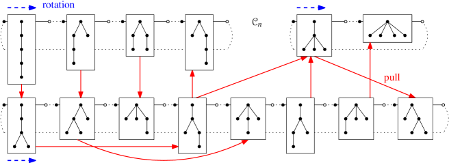
Figure 1: Cycle structure of the 2-factor ${\mathcal{C}}_{n}$ and auxiliary graph ${\mathcal{H}}_{n}$ for $n=4$.

The interpretation of the cycles of ${\mathcal{C}}_{n}$ in terms of rooted trees is illustrated in Figure 1 (ignore the solid arrows for the moment).

Proof.

To prove (i), let ${\mathcal{C}}_{n}^{-}$ denote the spanning subgraph of ${\mathcal{G}}_{n}$ obtained from ${\mathcal{C}}_{n}$ by removing the edges that flip the last bit. As ${\mathcal{C}}_{n}$ is a union of cycles, ${\mathcal{C}}_{n}^{-}$ is a union of paths ${\mathcal{P}}_{n}\circ 0$, ${\mathcal{P}}_{n}^{\prime}\circ 1$ and possibly some cycles ${\mathcal{R}}_{n}\circ 0$, ${\mathcal{R}}_{n}^{\prime}\circ 1$. Consider the automorphism $f(x_{1},\ldots,x_{2n+1}):=(\overline{\operatorname{rev}}(x_{1},\ldots,x_{2n}),\overline{x_{2n+1}})$ of the graph $G_{n}$. It is easy to check that $f(M)=M$ and $f(N)=N$, implying that ${\mathcal{P}}_{n}^{\prime}=\overline{\operatorname{rev}}({\mathcal{P}}_{n})$ and ${\mathcal{R}}_{n}^{\prime}=\overline{\operatorname{rev}}({\mathcal{R}}_{n})$, so we have

$${\mathcal{C}}_{n}^{-}=({\mathcal{P}}_{n}\cup{\mathcal{R}}_{n})\circ 0\;\cup\;\overline{\operatorname{rev}}({\mathcal{P}}_{n}\cup{\mathcal{R}}_{n})\circ 1\enspace.$$ (3)

This almost proves (i). The only thing left to verify is that ${\mathcal{R}}_{n}=\emptyset$, which will be done later.

To prove (ii)–(iv), consider an end vertex $x$ of a path from ${\mathcal{P}}_{n}$. It corresponds to a vertex $(x,0)\in B_{n}$ such that either $M$ or $N$ flips the last bit of $(x,0)$. By the definition of $M$ and $N$, this happens if and only if $x\in D_{n}^{-}$ or $x\in D_{n}$, respectively. Consequently, the end vertices of ${\mathcal{P}}_{n}$ are given by $D_{n}\cup D_{n}^{-}$.

Now consider a path $P\in{\mathcal{P}}_{n}$ with end vertex $x\in D_{n}$, and let $x=(1,u,0,v)$ be the canonic decomposition of $x$. We now show that $P=P_{\sigma}(x)$. Note that every recursion step in the definition (2) corresponds to a pair of indices $1\leq a<b\leq|u|+2$ in $x$ such that $(x_{a},\ldots,x_{b})=(1,w^{\prime},0)$ with $w^{\prime}\in D$. We refer to such a pair $(a,b)$ as a base pair of $x$. For any such base pair $(a,b)$, we can partition $x$ uniquely as

$$x=(1,u_{1},1,u_{2},\ldots,1,u_{d},1,w^{\prime},0,v_{d},0,v_{d-1},0,\ldots,v_{1},0,v)$$ (4)

with $d\geq 0$ and $u_{1},\ldots,u_{d},v_{1},\ldots,v_{d}\in D$, see Figure 2. Note that $a=1+\sum_{i=1}^{d}(1+|u_{i}|)$ and $b=a+|w^{\prime}|+1$. Let $x^{\prime}$ and $x^{\prime\prime}$ denote the entries of the sequence $P_{\sigma}(x)$ at positions $2a-1$ and $2b-1$, respectively. These are well-defined vertices as $\sigma(x)$ has length $2|u|+2$ by definition (2) and by the inequality $a<b\leq|u|+2$. Using definition (2), a straightforward computation shows that for any base pair $(a^{\prime},b^{\prime})$ and the corresponding substring $(1,u^{\prime},0)\in D$ of $x$, applying the bitflips in $\sigma(x)$ to this substring, every bit $x_{i}$ followed by $x_{i+1}=x_{i}$ is flipped twice, whereas every bit $x_{i}$ followed by $x_{i+1}=\overline{x_{i}}$ is flipped once or three times, depending on whether $x_{i}=1$ or $x_{i}=0$, respectively. This effectively shifts the bitstring to the left, yielding $(u^{\prime},0,x_{b^{\prime}+1})$. Using this observation, the vertices $x^{\prime}$ and $x^{\prime\prime}$ can be computed from (4) as

$$x^{\prime} =(u_{1},0,u_{2},0,\ldots,u_{d},0,1,w^{\prime},0,v_{d},1,v_{d-1},1,\ldots,v_{1},1,v)\enspace,$$ (5a)

$$x^{\prime\prime} =(u_{1},0,u_{2},0,\ldots,u_{d},0,w^{\prime},0,1,v_{d},1,v_{d-1},1,\ldots,v_{1},1,v)\enspace.$$ (5b)

By (2a) and (2b), the next two bits flipped after $x^{\prime}$ are at positions $b$ and $a$. Using (5a) and the definition of the mappings $M$ and $N^{-1}$, these are exactly the two bits flipped along the edge from $M$ that starts at $(x^{\prime},0)\in B_{n}$ and along the edge from $N$ that starts at $M(x^{\prime},0)\in B_{n}^{\prime}$, respectively. Similarly, if $b<|u|+2$, then by (2b), the next two bits flipped after $x^{\prime\prime}$ are at positions $a-1$ and $b$. Using (5b) and the definition of $M$ and $N^{-1}$, these are exactly the two bits flipped along the edge from $M$ that starts at $(x^{\prime\prime},0)\in B_{n}$ and along the edge from $N$ that starts at $M(x^{\prime\prime},0)\in B_{n}^{\prime}$, respectively. As this argument holds for all base pairs $(a,b)$ of $x$, we obtain $P=P_{\sigma}(x)$, proving (iii). Applying (5b) for the base pair $(a,b)=(1,|u|+2)$ of $x$ (in this case $d=0$ and $w^{\prime}=u$), the last vertex $y$ reached on the path $P=P_{\sigma}(x)$ is $y=(u,0,1,v)\in D_{n}^{-}$. This proves (ii). Recall that $|\sigma(x)|=2|u|+2$, so the distance between $x$ and $y$ along $P$ is $2|u|+2$, proving (iv).

To prove (v), consider a path $P\in{\mathcal{P}}_{n}$ with first vertex $x=(1,u,0,v)\in D_{n}$, where $u,v\in D$, and last vertex $y^{\prime}:=(u,0,1,v)\in D_{n}^{-}$. We consider the cycle $C\in{\mathcal{C}}_{n}$ containing the path $P\circ 0$ and continue to follow this cycle. The next edge of $C$ after traversing $P\circ 0$ flips the last bit, so from $(y^{\prime},0)$ we reach the vertex $(y^{\prime},1)$. By (3), the path traversed by $C$ until the last bit is flipped again is $\overline{\operatorname{rev}}(P^{\prime})\circ 1$ for some $P^{\prime}\in{\mathcal{P}}_{n}$. As the last vertex of $P^{\prime}$ is $\overline{\operatorname{rev}}(y^{\prime})=(\overline{\operatorname{rev}}(v),0,1,\overline{\operatorname{rev}}(u))\in D_{n}^{-}$, its first vertex is $x^{\prime}:=(1,\overline{\operatorname{rev}}(v),0,\overline{\operatorname{rev}}(u))\in D_{n}$ by (iv). As the path $\overline{\operatorname{rev}}(P^{\prime})\circ 1$ is traversed backwards by $C$, the next vertex on $C$ after traversing $\overline{\operatorname{rev}}(P^{\prime})\circ 1$ is $(y,0)$ with $y:=\overline{\operatorname{rev}}(x^{\prime})=(u,1,v,0)\in D_{n}$. The distance between $(x,0)$ and $(y,0)$ along $C$ is $(2|u|+2)+(2|v|+2)+2$ by (iv), which equals $2(|u|+|v|+2)+2=4n+2$. This almost proves (v), assuming that ${\mathcal{R}}_{n}=\emptyset$ in (3). However, the total number of vertices visited by the paths ${\mathcal{P}}_{n}\circ 0$ and $\overline{\operatorname{rev}}({\mathcal{P}}_{n})\circ 1$ is $(4n+2)|D_{n}|$. As the cardinality of $D_{n}$ is given by the $n$-th Catalan number [Sta15], this quantity equals $2\binom{2n+1}{n}$, the total number of vertices of $G_{n}$. It follows that ${\mathcal{R}}_{n}=\emptyset$ in (3), completing the proofs of (i) and (v).

Claim (vi) is an immediate consequence of (ii), (v), and the definition of plane trees. ∎

4 Properties of the 6-cycles

Proposition 3 below states all relevant properties of the set of 6-cycles ${\mathcal{S}}_{n}$ that we use. To state the proposition, we say that $x,y\in D_{n}$ form a flippable pair $(x,y)$, if

$$x =(1,u_{1},1,u_{2},\ldots,1,u_{d},1,1,0,w,0,v_{d},0,v_{d-1},0,\ldots,v_{1},0,v_{0})\enspace,$$ (6)

$$y =(1,u_{1},1,u_{2},\ldots,1,u_{d},1,0,1,w,0,v_{d},0,v_{d-1},0,\ldots,v_{1},0,v_{0})$$

for some $d\geq 0$ and $u_{1},\ldots,u_{d},v_{0},\ldots,v_{d},w\in D$. In terms of rooted trees, the tree $y$ is obtained from $x$ by moving a pending edge from a vertex in the left subtree to its predecessor, see Figure 2. We refer to $(1,1,0,w,0)$ and $(1,0,1,w,0)$ as flippable substrings of $x$ and $y$ corresponding to this flippable pair. The corresponding subpaths are highlighted with gray boxes in the figure. Note that a bitstring $x$ may appear in multiple flippable pairs, as it may contain multiple flippable substrings.

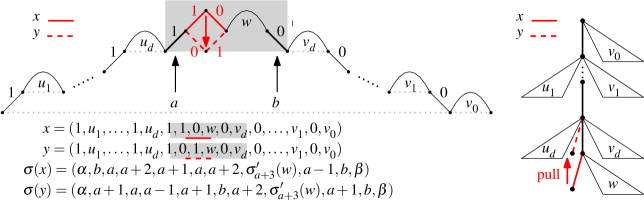
Figure 2: A flippable pair $(x,y)$, its Dyck path interpretation (left) and rooted tree interpretation (right).

Clearly, the set of 6-cycles ${\mathcal{S}}_{n}$ defined in Section 1.1 is given by considering all flippable pairs $(x,y)$, $x,y\in D_{n}$, as in (6), by defining

$$C_{6}(x,y):=(u_{1},0,u_{2},0,\ldots,u_{d},0,1,*,*,w,*,v_{d},1,v_{d-1},1,\ldots,v_{1},1,v_{0})$$ (7)

and by taking the union of all 6-cycles $C_{6}(x,y)\circ 0$. Note here that (1) and (7) differ only in the additional 0-bit in the end. In particular, all 6-cycles ${\mathcal{S}}_{n}$ that we use to join the cycles in the 2-factor ${\mathcal{C}}_{n}$ belong to the subgraph of $G_{n}$ given by all vertices whose last bit equals 0.

Proposition 3.

For any $n\geq 1$, the 6-cycles $C_{6}(x,y)$ defined in (7) have the following properties:

1. Let $(x,y)$ be a flippable pair. The symmetric difference of the edge sets of the two paths $P_{\sigma}(x)$ and $P_{\sigma}(y)$ with the 6-cycle $C_{6}(x,y)$ gives two paths $P^{\prime}(x)$ and $P^{\prime}(y)$ on the same set of vertices as $P_{\sigma}(x)$ and $P_{\sigma}(y)$, where $P^{\prime}(x)$ starts at $x$ and ends at the last vertex of $P_{\sigma}(y)$, and $P^{\prime}(y)$ starts at $y$ and ends at the last vertex of $P_{\sigma}(x)$.

2. Let $(x,y)$ be a flippable pair and let $a$ be the starting position of the corresponding flippable substring in $x$. The 6-cycle $C_{6}(x,y)$ intersects $P_{\sigma}(x)$ in the $(2a-1)$-th and the $(2a+4)$-th edge, and it intersects $P_{\sigma}(y)$ in the $(2a-1)$-th edge.

3. For any flippable pairs $(x,y)$ and $(x^{\prime},y^{\prime})$, the 6-cycles $C_{6}(x,y)$ and $C_{6}(x^{\prime},y^{\prime})$ are edge-disjoint.

4. For any flippable pairs $(x,y)$ and $(x,y^{\prime})$, the two pairs of edges that the two 6-cycles $C_{6}(x,y)$ and $C_{6}(x,y^{\prime})$ have in common with the path $P_{\sigma}(x)$ are not interleaved, but one pair appears before the other pair along the path.

Informally, the first property asserts that a 6-cycle from ${\mathcal{S}}_{n}$ can be used to join two cycles from the 2-factor ${\mathcal{C}}_{n}$ to a single cycle, see Figure 3. The last two properties ensure that no two 6-cycles interfere with each other when iterating this joining operation.

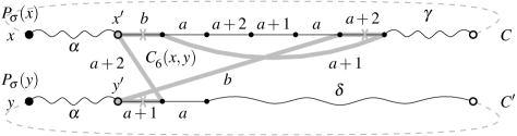
Figure 3: Two cycles from our 2-factor joined by taking the symmetric difference with a 6-cycle. The paths $P_{\sigma}(x)$ and $P_{\sigma}(y)$ (solid black) lying on the two cycles traverse the 6-cycle $C_{6}(x,y)$ (solid gray) as shown. The symmetric difference yields paths $P^{\prime}(x)=P(x,\tau(x))$ and $P^{\prime}(y)=P(y,\tau(y))$ that have flipped end vertices.

Proof.

To prove (i), consider a flippable pair $(x,y)$ as in (6), and let $a$ and $b$ be the first and last position of the corresponding flippable substring $(1,1,0,w,0)$ in $x$, respectively. Applying the definition (2), a straightforward computation yields the bitflip sequences

$$\sigma(x) =(\alpha,b,a,a+2,a+1,a,a+2,\gamma)\enspace,$$ (8a)

$$\sigma(y) =(\alpha,a+1,a,\delta)\enspace,$$

where if $$d=0$$ we define

$$\alpha:=\beta:=\delta:=()\;\;\text{and}\;\;\gamma:=(\sigma_{a+3}(w))\enspace.$$ (8b)

On the other hand, if $$d>0 \alpha \sigma(x) \sigma(y) (b,\beta)$$ then  is the longest common prefix of  and , is their longest common suffix, and

$$\gamma:=(\sigma_{a+3}(w),a-1,b,\beta)\;\;\text{and}\;\;\delta:=(a-1,a+1,b,a+2,\sigma_{a+3}(w),a+1,b,\beta)\enspace.$$ (8c)

Note that $(\alpha,\beta)=\sigma(1,u_{1},1,u_{2},\ldots,1,u_{d},v_{d},0,v_{d-1},0,\ldots,v_{1},0)$ and that $|\alpha|=2(d+\sum_{i=1}^{d}|u_{i}|)=2(a-1)=2a-2$. The last relation expresses that we count two flip operations for each of the steps from the hills $u_{1},u_{2},\ldots,u_{d}$, one flip for each of the $d$ upsteps preceding the hills $u_{i}$, and one flip for each of the $d$ downsteps following the hills $v_{i}$. Specifically, the vertices $x^{\prime}$ and $y^{\prime}$ that are reached from $x$ or $y$ by flipping all $2a-2$ bit positions in the sequence $\alpha$ are

$$x^{\prime} =(u_{1},0,u_{2},0,\ldots,u_{d},0,1,1,0,w,0,v_{d},1,v_{d-1},1,\ldots,v_{1},1,v_{0})\enspace,$$ (9)

$$y^{\prime} =(u_{1},0,u_{2},0,\ldots,u_{d},0,1,0,1,w,0,v_{d},1,v_{d-1},1,\ldots,v_{1},1,v_{0})\enspace.$$

Comparing (7) and (9) shows that these vertices belong to the 6-cycle $C_{6}(x,y)$. From (8a) we observe that the 6-cycle $C_{6}(x,y)$ is then traversed as depicted in Figure 3. In particular, $x^{\prime}$ and $y^{\prime}$ are the first vertices from the paths $P_{\sigma}(x)$ and $P_{\sigma}(y)$ hitting the 6-cycle. By taking the symmetric difference of these edge sets, we obtain paths $P^{\prime}(x)$ and $P^{\prime}(y)$ on the same vertex set as $P_{\sigma}(x)$ and $P_{\sigma}(y)$ with flipped end vertices. Formally, $P^{\prime}(x)$ and $P^{\prime}(y)$ are obtained by starting at $x$ and $y$ and flipping bits according to the modified bitflip sequences

$$\tau(x) :=(\alpha,a+2,a,\delta)\enspace,$$

$$\tau(y) :=(\alpha,b,a,a+1,a+2,a,a+1,\gamma)\enspace,$$

respectively. This proves (i).

Recall from the previous argument that the distance between $x$ and $x^{\prime}$ along the path $P_{\sigma}(x)$ is $|\alpha|=2a-2$, and the same holds for the distance between $y$ and $y^{\prime}$ along the path $P_{\sigma}(y)$. The 6-cycle $C_{6}(x,y)$ intersects $P_{\sigma}(x)$ in the next edge after $x^{\prime}$ and in the edge that is five edges further away, and it intersects $P_{\sigma}(y)$ in the next edge after $y^{\prime}$. Combining these facts proves (ii).

To prove (iii), consider two 6-cycles $C_{6}(x,y)$ and $C_{6}(x^{\prime},y^{\prime})$. Instead of comparing them directly, we consider how they intersect a fixed path $P_{\sigma}(z)$ with $z\in\{x,y\}\cap\{x^{\prime},y^{\prime}\}$. This is possible because all edges of these 6-cycles either lie on such a path or they go between two such paths. Consider the two flippable substrings of $z$ corresponding to $C_{6}(x,y)$ and $C_{6}(x^{\prime},y^{\prime})$ starting at positions $a$ and $a^{\prime}$ in $z$, respectively. We assume w.l.o.g. that $a^{\prime}\geq a+1$.

We first consider the case $z=y$ and $z\in\{x^{\prime},y^{\prime}\}$. By (ii) we know that the 6-cycle $C_{6}(x,y)$ intersects the path $P_{\sigma}(y)$ in the edge $2a-1$. However, we also have $2a^{\prime}-1\geq 2(a+1)-1=2a+1$, so the edge(s) that the cycle $C_{6}(x^{\prime},y^{\prime})$ has in common with $P_{\sigma}(y)$ are separated by at least one edge along the path, proving that the two 6-cycles do not share any vertices on this path.

We now consider the case $z=x$ and $z\in\{x^{\prime},y^{\prime}\}$. By (ii) we know that the 6-cycle $C_{6}(x,y)$ intersects the path $P_{\sigma}(x)$ in the edges $2a-1$ and $2a+4$. If $a^{\prime}\geq a+4$, then we have $2a^{\prime}-1\geq 2(a+4)-1=2a+7$, so the edges that the cycle $C_{6}(x^{\prime},y^{\prime})$ has in common with $P_{\sigma}(x)$ are separated by at least two edges along the path, proving that the two 6-cycles do not share any vertices on this path. It remains to consider the subcases $a^{\prime}\in\{a+1,a+2,a+3\}$. The case $a^{\prime}=a+2$ can be excluded, because this would mean that $x$ has a 0-bit at position $a+2$ and $x$ has a 1-bit at position $a^{\prime}=a+2$ by (6), which is a contradiction. If $a^{\prime}=a+1$, then since $x$ has a 0-bit at position $a+2$, it follows from (6) that $y^{\prime}=x$ and that the flippable substring of $x$ corresponding to $(x,y)$ has the form $(1,1,0,w,0)=(1,1,0,1,w^{\prime},0,0)$. Consequently, by (ii) $C_{6}(x^{\prime},y^{\prime})$ intersects the path $P_{\sigma}(x)$ in the edge $2a^{\prime}-1=2(a+1)-1=2a+1$, which is separated by at least one edge from both edges $2a-1$ and $2a+4$, so the two 6-cycles do not share any vertices on this path. If $a^{\prime}=a+3$, then either of the two cases $x^{\prime}=x$ or $y^{\prime}=x$ can occur, and in both cases the cycle $C_{6}(x^{\prime},y^{\prime})$ intersects $P_{\sigma}(x)$ in the edge $2a^{\prime}-1=2(a+3)-1=2a+5$, and if $x^{\prime}=x$ also in the edge $2a^{\prime}+4=2a+10$ (which is safe for sure). The edge $2a+5$ is different from the edge $2a+4$ on $P_{\sigma}(x)$, but both share an end vertex, so the other two edges of the 6-cycles $C_{6}(x,y)$ and $C_{6}(x^{\prime},y^{\prime})$ starting at this vertex and not belonging to $P_{\sigma}(x)$ could be identical. However, this is not the case as the corresponding edge from $C_{6}(x,y)$ leads back to $P_{\sigma}(x)$, whereas the corresponding edge from $C_{6}(x^{\prime},y^{\prime})$ leads to $P_{\sigma}(y^{\prime})$ if $x^{\prime}=x$ and to $P_{\sigma}(x^{\prime})$ if $y^{\prime}=x$.

This completes the proof of (iii).

The previous analysis in the last case where $z=x=x^{\prime}$ also proves (iv). ∎

5 Proof of Theorem 1

With Propositions 2 and 3 in hand, we are now ready to prove Theorem 1.

Proof of Theorem 1.

Let ${\mathcal{C}}_{n}$ and ${\mathcal{S}}_{n}$ be the 2-factor and the set of 6-cycles defined in Section 1.1.

Consider two different cycles $C,C^{\prime}\in{\mathcal{C}}_{n}$ containing paths $P\circ 0\subseteq C$ and $P^{\prime}\circ 0\subseteq C^{\prime}$, where $P,P^{\prime}\in{\mathcal{P}}_{n}$, with first vertices $x,y\in D_{n}$, respectively, such that $(x,y)$ is a flippable pair. By Proposition 3 (i), the symmetric difference of the edge sets $(C\cup C^{\prime})\bigtriangleup(C_{6}(x,y)\circ 0)$ forms a single cycle on the same vertex set as $C\cup C^{\prime}$, i.e., this joining operation reduces the number of cycles in the 2-factor by one, see Figure 3. Recall from (6) that in terms of rooted trees, the tree $y$ is obtained from $x$ by moving a pending edge from a vertex in the left subtree to its predecessor. We refer to this as a pull operation, see Figure 2.

We repeat this joining operation until all cycles in the 2-factor are joined to a single Hamilton cycle. For this purpose we define an auxiliary graph ${\mathcal{H}}_{n}$ whose nodes represent the cycles in the 2-factor ${\mathcal{C}}_{n}$ and whose edges connect pairs of cycles that can be connected to a single cycle with such a joining operation that involves a 6-cycle from the set ${\mathcal{S}}_{n}$, see Figure 1. Formally, the node set of ${\mathcal{H}}_{n}$ is given by partitioning the set of all rooted trees with $n$ edges into equivalence classes under tree rotation. By Proposition 2 (v) and (vi), each cycle $C$ of ${\mathcal{C}}_{n}$ can be identified with one equivalence class under tree rotation, so the nodes of ${\mathcal{H}}_{n}$ indeed correspond to the cycles in the 2-factor ${\mathcal{C}}_{n}$. Specifically, each rooted tree belonging to some node of ${\mathcal{H}}_{n}$ equals the first vertex $x\in D_{n}$ of some path $P\in{\mathcal{P}}_{n}$ such that $P\circ 0$ lies on the cycle corresponding to that node. For every flippable pair $(x,y)$, $x,y\in D_{n}$, we add the edge to ${\mathcal{H}}_{n}$ that connects the node containing the tree $x$ to the node containing the tree $y$. In Figure 1, those edges are drawn as solid arrows directed from $x$ to $y$. By our initial argument, such a flippable pair yields a 6-cycle $C_{6}(x,y)$ that can be used in $G_{n}$ to join the two corresponding cycles to a single cycle. Note that ${\mathcal{H}}_{n}$ may contain multiple edges or loops.

To complete the proof, it therefore suffices to prove that the graph ${\mathcal{H}}_{n}$ is connected. Indeed, if ${\mathcal{H}}_{n}$ is connected, then we can pick a spanning tree in ${\mathcal{H}}_{n}$, corresponding to a collection of 6-cycles ${\mathcal{T}}_{n}\subseteq{\mathcal{S}}_{n}$, such that the symmetric difference between the edge sets ${\mathcal{C}}_{n}\bigtriangleup{\mathcal{T}}_{n}$ forms a Hamilton cycle in $G_{n}$. Here we need properties (iii) and (iv) in Proposition 3, which ensure that whatever subset of 6-cycles we use in this joining process, they will not interfere with each other, guaranteeing that inserting each 6-cycle indeed reduces the number of cycles by one, as desired.

At this point we have reduced the problem of proving that $G_{n}$ has a Hamilton cycle to showing that the auxiliary graph ${\mathcal{H}}_{n}$ is connected, which is much easier. Indeed, all we need to show is that any rooted tree with $n$ edges can be transformed into any other tree by a sequence of rotations and pulls, and their inverse operations. Recall that rotations correspond to following the same cycle from ${\mathcal{C}}_{n}$ (staying at the same node in ${\mathcal{H}}_{n}$), and a pull corresponds to a joining operation (traversing an edge in ${\mathcal{H}}_{n}$ to another node). For this we show that any rooted tree $x$ can be transformed into the special tree $s:=(1,1,0,1,0,\ldots,1,0,0)\in D_{n}$, i.e., a star with $n$ rays rooted at a leaf, by a sequence of rotations and pulls. This can be achieved by rotating $x$ until it is rooted at a leaf. Now the left subtree is the entire tree, so we can repeatedly pull pending edges towards the unique child of the root until we end up at the star $s$.

This completes the proof. ∎

References

- [BW84] M. Buck and D. Wiedemann. Gray codes with restricted density. Discrete Math., 48(2-3):163–171, 1984.
- [DG12] P. Diaconis and R. Graham. Magical mathematics. Princeton University Press, Princeton, NJ, 2012. The mathematical ideas that animate great magic tricks, With a foreword by Martin Gardner.
- [DKS94] D. A. Duffus, H. A. Kierstead, and H. S. Snevily. An explicit -factorization in the middle of the Boolean lattice. J. Combin. Theory Ser. A, 65(2):334–342, 1994.
- [FT95] S. Felsner and W. T. Trotter. Colorings of diagrams of interval orders and -sequences of sets. Discrete Math., 144(1-3):23–31, 1995. Combinatorics of ordered sets (Oberwolfach, 1991).
- [GJM+18] P. Gregor, S. Jäger, T. Mütze, J. Sawada, and K. Wille. Gray codes and symmetric chains. To appear in Proceedings of the 45th International Colloqium on Automata, Languages and Programming (ICALP 2018). arXiv:1802.06021, 2018.
- [GM18] P. Gregor and T. Mütze. Trimming and gluing Gray codes. Theoret. Comput. Sci., 714:74–95, 2018.
- [Gow17] W. T. Gowers. Probabilistic combinatorics and the recent work of Peter Keevash. Bull. Amer. Math. Soc. (N.S.), 54(1):107–116, 2017.
- [Hav83] I. Havel. Semipaths in directed cubes. In Graphs and other combinatorial topics (Prague, 1982), volume 59 of Teubner-Texte Math., pages 101–108. Teubner, Leipzig, 1983.
- [Joh04] J. R. Johnson. Long cycles in the middle two layers of the discrete cube. J. Combin. Theory Ser. A, 105(2):255–271, 2004.
- [Knu11] D. E. Knuth. The Art of Computer Programming. Vol. 4A. Combinatorial Algorithms. Part 1. Addison-Wesley, Upper Saddle River, NJ, 2011.
- [KT88] H. A. Kierstead and W. T. Trotter. Explicit matchings in the middle levels of the Boolean lattice. Order, 5(2):163–171, 1988.
- [Lov70] L. Lovász. Problem 11. In Combinatorial Structures and Their Applications (Proc. Calgary Internat. Conf., Calgary, Alberta, 1969). Gordon and Breach, New York, 1970.
- [MN17] T. Mütze and J. Nummenpalo. A constant-time algorithm for middle levels Gray codes. In Proceedings of the Twenty-Eighth Annual ACM-SIAM Symposium on Discrete Algorithms, pages 2238–2253. SIAM, Philadelphia, PA, 2017.
- [MNW18] T. Mütze, J. Nummenpalo, and B. Walczak. Sparse Kneser graphs are Hamiltonian. To appear in Proceedings of the 50th Annual ACM Symposium on the Theory of Computing (STOC 2018). arXiv:1711.01636, 2018.
- [MS17] T. Mütze and P. Su. Bipartite Kneser graphs are Hamiltonian. Combinatorica, 37(6):1207–1219, 2017.
- [MSW18] T. Mütze, C. Standke, and V. Wiechert. A minimum-change version of the Chung-Feller theorem for Dyck paths. European J. Combin., 69:260–275, 2018.
- [Müt16] T. Mütze. Proof of the middle levels conjecture. Proc. Lond. Math. Soc., 112(4):677–713, 2016.
- [Sav93] C. D. Savage. Long cycles in the middle two levels of the Boolean lattice. Ars Combin., 35(A):97–108, 1993.
- [Sta15] R. P. Stanley. Catalan numbers. Cambridge University Press, New York, 2015.
- [SW95] C. D. Savage and P. Winkler. Monotone Gray codes and the middle levels problem. J. Combin. Theory Ser. A, 70(2):230–248, 1995.
- [Win04] P. Winkler. Mathematical puzzles: a connoisseur’s collection. A K Peters, Ltd., Natick, MA, 2004.