Feature learning in feature–sample networks using multi-objective optimization

Abstract

Data and knowledge representation are fundamental concepts in machine learning. The quality of the representation impacts the performance of the learning model directly. Feature learning transforms or enhances raw data to structures that are effectively exploited by those models. In recent years, several works have been using complex networks for data representation and analysis. However, no feature learning method has been proposed for such category of techniques. Here, we present an unsupervised feature learning mechanism that works on datasets with binary features. First, the dataset is mapped into a feature–sample network. Then, a multi-objective optimization process selects a set of new vertices to produce an enhanced version of the network. The new features depend on a nonlinear function of a combination of preexisting features. Effectively, the process projects the input data into a higher-dimensional space. To solve the optimization problem, we design two metaheuristics based on the lexicographic genetic algorithm and the improved strength Pareto evolutionary algorithm (SPEA2). We show that the enhanced network contains more information and can be exploited to improve the performance of machine learning methods. The advantages and disadvantages of each optimization strategy are discussed.

I Introduction

A good representation of the encoded knowledge in a machine learning model is fundamental to its success. Several data structures have been used for this purpose, for instance, matrices of weights, trees, and graphs [1, 2]. Sometimes, learning models lack a data structure to store knowledge, storing the input as is [3].

In recent years, several works have been using complex networks for data representation and analysis [4, 5, 6]. Complex networks are graphs with a nontrivial topology that represent the interactions of a dynamical system [7]. Advances in the science of complex systems bring several tools to understand such systems.

In [8], we describe how to map a dataset with binary features into a bipartite complex-network. Such network is called feature–sample network. Using that representation, we solve a semi-supervised learning task called positive-unlabeled (PU) learning [9].

When dealing with machine learning problems, we often need to pre-process the input data. Feature learning transforms or enhances raw data to structures that are effectively exploited by learning models. Autoencoders and manifold learning are examples of feature learning methods [10].

In this paper, we propose a feature learning process to add information in feature–sample networks. In summary, we include to the network a limited number of new vertices based on a non-linear function of the preexisting ones. The set of new vertices is determined by a multi-objective objective problem, in which the goal is to maximize the number of features while maintaining some properties of the original data. Two multi-objective approaches are designed: a lexicographic genetic algorithm (LGA) and an implementation of the improved strength Pareto evolutionary algorithm (SPEA2).

We show that enhanced feature–sample networks improve the performance of learning methods in the major machine learning paradigms: supervised and unsupervised learning. We also expose the pros and cons of each optimization approach.

The rest of this paper is organized as follows. Sections II and III describe how to enhance feature–sample networks as an optimization problem. In Section IV, computer simulations illustrate the optimization process and assess the performance improvements in machine learning tasks. Finally, we conclude this paper in Section V.

II Enhanced feature–sample networks

In this section, we describe how we enhance a feature–sample network by adding to the network a constrained number of new features. Connections between the samples and each new feature depend on a nonlinear function of a combination of preexisting features. The chosen set of new features is the result of an optimization process that not only maximizes the number of new features but also distributes them along the samples. This process is similar to the projection of the associated data into a higher-dimensional space preserving some important characteristics of the data.

In the following subsections, we first review the feature–sample networks, then describe the creation of new features. Moreover, we elaborate an optimization problem to enhance feature–sample networks.

II-A Feature–sample network review

Assume as input the dataset $\mathcal{B}=\{\vec{x}_{1},\ldots,\vec{x}_{N}\}$ whose members are binary feature vectors $\vec{x}_{i}=[x_{i1},\dots,x_{iD}]\in\{0,1\}^{D}$. The feature vectors are sparse, that is, the number of elements with value 1 is much lower than the dimension $D$.

The feature–sample network $\mathcal{G}$ is the bipartite complex-network whose edges connect samples and features of the dataset $\mathcal{B}$. A simple, unweighted, undirected graph $(\mathcal{V},\mathcal{E})$ represents such network. The vertex set $\mathcal{V}$ is $\{v_{1},\dots,v_{N},v_{N+1},\dots,v_{N+D}\}$ and an edge exists between sample $v_{i}$ and feature $v_{N+j}$ if $x_{ij}=1$.

II-B And-features definition

According to the Cover’s Theorem [3], given a not-densely populated space of a classification problem, the chance of it being linearly separable is increased as one cast it in a high-dimensional space nonlinearly.

Since we assume the input feature–sample network is sparse, we can synthesize features nonlinearly to exploit the properties of this theorem. One way to produce new features is using the and operator, which is a nonlinear Boolean function.

We call and-feature the feature $v$ that links to all samples connected to a given set of two or more preexisting features.

Given a feature–sample network $\mathcal{G}$ with $N$ samples and $D$ features, we can produce an and-feature $v$ for each combination $\mathcal{W}$ of $q$ features such that $\left|\mathcal{W}\right|\geq 2$ and $\mathcal{W}\subseteq\{v_{N+1},\dots,v_{N+D}\}$. We call $q$ the order of the and-feature $v$. Thus, the number of possible and-features is

$$\sum_{q=2}^{D}{D\choose q}=\sum_{q=2}^{D}{\frac{D!}{q!\left(D-q\right)!}}=2^{D}-D-1\text{.}$$

In the rest of this paper, we index every possible and-feature using the parameter $\vec{a}=[a_{1}$, …, $a_{D}]\in\{0,1\}^{D}$ such that $\sum_{j}{a_{j}}\geq 2$. Each element $a_{j}$ indicates a feature in the network. The feature $v_{N+j}$ is part of the combination if, and only if, $a_{j}=1$. Thus, the set $\mathcal{W}$ is $\{v_{N+j}\left|\right.a_{j}=1\}$.

Using this notation, we say that the and-feature $v(\vec{a})$ connects to each sample $v_{i}$ if, and only if, $\left(\lnot a_{1}\lor x_{i1}\right)\land\dots\land\left(\lnot a_{D}\lor x_{iD}\right)=1$ holds.

From this discussion, we realize that enumerating every combination has exponential cost. Moreover, once the network is sparse, we expect that many of the and-features have no connections.

II-C Optimization problem definition

The problem of enhancing the network can be viewed as a optimization problem. Given an input feature–sample network $\mathcal{G}$ with $N$ samples and $D$ features, we denote $\mathcal{G}(\mathcal{Y})$ the enhanced network from the original $\mathcal{G}$ by adding every and-feature $v\in\mathcal{Y}$. The number of features of the enhanced network, excluding the and-features that do not connect, is given by $D(\mathcal{Y})$. Thus, $\mathcal{G}=\mathcal{G}(\varnothing)$ and $D=D(\varnothing)$.

Let $M_{\text{max}}$ be the maximum number allowed of generated features, we want to

$$\underset{\mathcal{Y}}{\text{minimize}} D(\varnothing)-D(\mathcal{Y})$$

subject to $$D(\mathcal{Y})-D(\varnothing)\leq M_{\text{max}}\text{.}$$

The disadvantage of this approach is that the and-features might not be well distributed. Thus, while some samples may have few new feature, others may have many. To overcome this limitation, we introduce the disproportion $\Delta(\mathcal{G},\mathcal{G}^{\prime})\in[0,\infty)$ between the network $\mathcal{G}$ and its enhanced version $\mathcal{G}^{\prime}$.

The disproportion is zero if the number of new connections in each sample is proportional to its initial sparsity. In this way, while the sparsity of each sample might change, we keep the same shape of the degree distribution of the samples.

Let $k_{i}$ be the degree of the sample $v_{i}$, the disproportion between two networks is

$$\Delta(\mathcal{G},\mathcal{G}^{\prime})=\mathrm{sd}\!\left(\frac{k_{1}(\mathcal{G}^{\prime})-k_{1}(\mathcal{G})}{k_{1}(\mathcal{G})},\dots,\frac{k_{N}(\mathcal{G}^{\prime})-k_{N}(\mathcal{G})}{k_{N}(\mathcal{G})}\right)\text{,}$$

where $\mathrm{sd}$ is the standard deviation of the arguments.

Using the disproportion in our optimization problem, the goal is to

$$\underset{\mathcal{Y}}{\text{minimize}} D(\varnothing)-D(\mathcal{Y}),\leavevmode\nobreak\ \Delta\big{(}\mathcal{G}(\varnothing),\mathcal{G}(\mathcal{Y})\big{)}$$

subject to $$D(\mathcal{Y})-D(\varnothing)\leq M_{\mathrm{max}}\text{.}$$

III Methods

In this section, we study the multi-objective problem stated in the previous section and describe how we solve it.

III-A Problem study

In Section II-B, we see that the number of possible and-features scales exponentially in the number of features $D$. As a consequence, storing every possible and-feature is not feasible.

Furthermore, the number of candidate solutions is also exponential in the number of possible new features. Precisely, there are at the most

$$\sum_{m=1}^{2^{D}-D-1}{{2^{D}-D-1}\choose m}=\sum_{m=1}^{2^{D}-D-1}{\frac{\left(2^{D}-D-1\right)!}{m!\left(2^{D}-D-m-1\right)!}}$$

solutions $\mathcal{Y}$ to explore. We can not limit the size of the set $\mathcal{Y}$ by $M_{\text{max}}$ since many and-features may have no connection.

The three common approaches for solving multi-objective optimization problems are weighted-formula, lexicographic, and Pareto [11]. The first strategy transforms the problem into a single-objective one, usually by weighting each objective and adding them up. The lexicographic approach assigns a priority to each objective and then optimizes the objectives in that order. Hence, when comparing two candidate solutions, the highest-priority objective is compared and, if equivalent, the second objective is compared. If the second objective is also equivalent between the solutions, the third one is used, and so on. Both the weighted-formula and the lexicographic strategies return only one solution for the problem. The Pareto methods use different mathematical tools to evaluate the candidate solution, finding a set of non-dominated solutions. A solution is said to be non-dominated if it is not worse than any other solution concerning all the criteria [11].

Since it is not trivial the difference of scale between our objective functions, we opted to use only a lexicographic and a Pareto method.

We design two population-based optimization algorithms. Specifically, we consider the use of two metaheuristics:

• a lexicographic genetic algorithm (GA); and

• the improved strength Pareto evolutionary algorithm (SPEA2) [12].

Although the methods are different, both approaches share many properties – individual representation, population initialization, operators of mutation, recombination and selection – which are explained in Section III-D. The main difference between them is the fitness evaluation.

In the GA, the individuals are ordered lexicographically, that is, ordered primarily by the first objective function and, in case of tie, the second objective. SPEA2, however, consider not only the Pareto front but also the density of the solutions.

III-B Lexicographic genetic algorithm review

A GA has the following steps [13]:

1:$X\leftarrow$ InitialPopulation()

2:while StopCondition() = false do

3:     Evaluate($X$)

4:     $X_{\text{next}}\leftarrow$ Elitism($X$)

5:     while $\left|X_{\text{next}}\right|<\left|X\right|$ do

6:         parents $\leftarrow$ Select($X$)

7:         children $\leftarrow$ Recombine(parents)

8:         Mutate(children)

9:         $X_{\text{next}}\leftarrow$ $X_{\text{next}}\cup$ children

10:     end while

11:     $X\leftarrow X_{\text{next}}$

12:end while.

In words, a random population of candidate solutions is generated as the first step. Then, while the stop condition is not met, the next generation of individuals comprises the best individuals of the previous generation and the individuals originated by recombining and mutating parents selected from the previous generation.

In the lexicographic approach, the only difference is during the evaluation of the candidate solution [14], where the best individuals are decided lexicographically.

In our specific problem, a solution $\mathcal{Y}_{1}$ is better than $\mathcal{Y}_{2}$ if

• $D(\mathcal{Y}_{1})>D(\mathcal{Y}_{1})$; or

• $D(\mathcal{Y}_{1})=D(\mathcal{Y}_{1})$ and $\Delta\big{(}\mathcal{G},\mathcal{G}(\mathcal{Y}_{1})\big{)}<\Delta\big{(}\mathcal{G},\mathcal{G}(\mathcal{Y}_{1})\big{)}$.

III-C Improved Strength Pareto Evolutionary Algorithm review

SPEA2 works similarly to a GA. The major difference is that it keeps an archive with the candidate solutions for the Pareto set. If the number of non-dominated solutions is greater than the limit of the archive, some solutions are discarded. Such operation is called truncation. The truncation operator tries to maintain the candidate solutions uniformly distributed along the Pareto front [12].

As indicated by the authors, we select individuals by employing binary tournament. Also, let $A$ be the archive size, we fix the parameter $k=\sqrt{\text{A}}$ in the truncation operator [12].

III-D Metaheuristic design

The common implementation characteristics of our metaheuristic is exposed in the next items.

III-D1 Individual representation

In our problem, each solution is a set $\mathcal{Y}$ of zero or more and-features. If we enumerate every possible and-feature, the solution can also be viewed as a binary vector with entries 1 for the present and-features.

III-D2 Population initialization

Given $\mu,\sigma>0$, we sample, without replacement, $\lfloor M\rfloor$ random and-features to compose each candidate solution $\mathcal{Y}$ such that $M\sim\mathcal{N}(\mu,\sigma)$. And-features are sampled so that the probability of having order $q\geq 2$ is

$$\frac{q-1}{q!}\text{.}$$

III-D3 Recombination operator

We use the uniform crossover operator with two parents generating two children. In Section III-D6, we show how to implement it efficiently using our set representation.

III-D4 Selection operator

The binary tournament method is chosen to select the parent that go to the recombination step.

III-D5 Mutation operator

We formulated the following specific mutation operator to exploit the characteristics of our problem.

Given a candidate solution $\mathcal{Y}$, we apply $\eta\in\{0,1,2,\dots\}$ random changes in the individual. For each change, there is a equal probability of either

• trying to add a new and-feature; or

• trying to remove an and-feature $v\in\mathcal{Y}$; or

• trying to modify an and-feature $v\in\mathcal{Y}$.

When trying to add a new feature, an and-feature $v$ is sampled and the solution is updated to $\mathcal{Y}\cup\{v\}$. Note that the candidate solution $\mathcal{Y}$ may not change if the and-feature was previously present.

If trying to remove a feature, each and-feature $v\in\mathcal{Y}$ has probability $\left(\left|\mathcal{Y}\right|+1\right)^{-1}$ of being selected. In this case, the candidate solution is updated to $\mathcal{Y}\setminus\{v\}$. Note that, with probability $\left(\left|\mathcal{Y}\right|+1\right)^{-1}$, the individual do not change.

Finally, in the last case, an and-feature $v(\vec{a})\in\mathcal{Y}$ with order $q=\sum_{j}{a_{j}}$ is selected uniformly to be modified. Once the and-feature is selected, a modified and-feature $v^{\prime}(\vec{a}^{\prime})$ will be produced. Two cases may happen: a) with chance $\frac{1}{q}$, an index $j^{\prime}\in[1,D]$ is selected uniformly, and $\vec{a}^{\prime}$ is $$\begin{dcases*}a^{\prime}_{j^{\prime}}=1&{}\\ a^{\prime}_{j}=a_{j}&$\forall j\neq j^{\prime}$\text{;}\end{dcases*}$$ b) with chance $\frac{q-1}{q}$, two indexes $j^{\prime}\in\{j\left|\right.a_{j}=1\}$ and $j^{\prime\prime}\in[1,D]$ are chosen uniformly. The modified and-feature is $$\begin{dcases*}a^{\prime}_{j^{\prime\prime}}=a_{j^{\prime}}&{}\\ a^{\prime}_{j^{\prime}}=a_{j^{\prime\prime}}&{}\\ a^{\prime}_{j}=a_{j}&$\forall j\not\in\{j^{\prime},j^{\prime\prime}\}$\end{dcases*}$$

The first case will include one more term into the and-feature if $a_{j^{\prime}}=0$. The second one swaps two elements of $\vec{a}$ and, effectively, takes effect when $a_{j^{\prime\prime}}=0$. The candidate solutions is then updated to $\left(\mathcal{Y}\setminus\{v\}\right)\cup\{v^{\prime}\}$. The size $\left|\mathcal{Y}\right|$ is never increased, and the candidate solution will be preserved if $v=v^{\prime}$.

III-D6 Performance considerations

Although, we can view both solutions and and-features as binary vectors, the set representation is more practical because of the high space-complexity of the problem. Moreover, there is no need to store entries for and-features that lack connections. Instead of just ignoring them, we exploit the evaluation step to determine which and-features are useless and remove them from the set.

Also, using the set representation, the crossover of the candidate solutions $\mathcal{Y}_{1}^{\text{parent}}$ and $\mathcal{Y}_{2}^{\text{parent}}$ can be implemented efficiently with steps

1:$\mathcal{Y}_{1}^{\text{child}},\mathcal{Y}_{2}^{\text{child}}\leftarrow\mathcal{Y}_{1}^{\text{parent}}\cup\mathcal{Y}_{2}^{\text{parent}}$

2:for $v\in\mathcal{Y}_{1}^{\text{parent}}\triangle\mathcal{Y}_{2}^{\text{parent}}$ do

3:     if SampleUniform($0$, $1$) ${}<0.5$ then

4:         $\mathcal{Y}_{1}^{\text{child}}\leftarrow\mathcal{Y}_{1}^{\text{child}}\cup\{v\}$

5:     else

6:         $\mathcal{Y}_{2}^{\text{child}}\leftarrow\mathcal{Y}_{2}^{\text{child}}\cup\{v\}$

7:     end if

8:end for

where $\triangle$ stands for the symmetric difference operator.

Finally, to conform to the requirements in Section III-D2, one can sample each candidate solution $\mathcal{Y}$ efficiently with steps

1:$v\leftarrow$ SampleAndFeature()

2:$\mathcal{Y}\leftarrow\{v\}$

3:loop

4:     $v\leftarrow$ SampleAndFeature()

5:     $\mathcal{Y}\leftarrow\mathcal{Y}\cup\{v\}$

6:     if SampleUniform($0$, $1$) ${}<1-\frac{1}{\left|\mathcal{Y}\right|}$ then

7:         break

8:     end if

9:end loop

where and-features are sampled without replacement.

IV Experimental results

In this section, we present applications of our feature learning technique in the two major categories in machine learning: supervised and unsupervised learning.

First, we illustrate the optimization process in the famous Iris dataset. In this example, we also conduct community detection in the original feature–sample network obtained from the dataset and in the enhanced one.

Then, we observe the increase of the accuracy obtained by the $k$-nearest neighbors [1] classifier in other four UCI datasets.

IV-A Enhanced community detection and clustering

The UCI Iris dataset [15] contains 150 samples that describe the sepals and petals of individual Iris flowers. The flowers are either Iris setosa, Iris virginica, or Iris versicolor. In [8], we construct a feature–sample network from this dataset by discretizing the features.

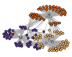
Figure 1: Feature–sample network for Iris dataset. Circles are vertices associated with samples and squares with features. Colors represent the classes.

Figure 1 shows the generated network. Each color represents a different class. Circles represent samples and squares, features. We use that same network as an input to both algorithms – using SPEA2 and the lexicographic GA.

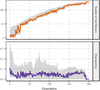
Figure 2: Evolution of the number of and-features and disproportion along the generations of the SPEA2 algorithm with Iris dataset as the input network. Solid lines are the average disproportion and number of and-features of the non-dominated solution at a given generation. Shadows cover the range of the measurements.

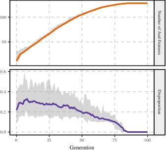
Figure 3: Evolution of the number of and-features and disproportion along the generations of the lexicographic GA with Iris dataset as the input network. Solid lines are the average disproportion and number of and-features of the best $100$ solutions (elitism) at a given generation. Shadows cover the range of the measurements.

IV-A1 Evolution of the candidate solutions

We execute the optimization process once for each strategy. We fix the population in $1000$ individuals. For SPEA2, the archive has size $100$ and, for the lexicographic GA, we keep the $100$ best solutions over the generations. In the initial population, we use $\mu=10$ and $\sigma=5$. The recombination rate is $0.6$ and the apply $\eta=1$ random changes in each generated individual.

Figures 2 and 3 describe the obtained result. Both disproportion and number of discovered and-feature are depicted along the generations. Solid lines are the average result in the population and shadows cover the range – from minimum to maximum – of each measurement. The results include only the non-dominated solutions in SPEA2 and the $100$ best solutions in the lexicographic GA.

Using both strategies, we could reach the optimal solution: $128$ and-features with at least one connection and $0$ disproportion. However, the optimization strategies differ as to how to achieve this.

SPEA2 tries to find as many new and-feature while keeping the ones with lowest values of disproportion. When a larger set of and-features with disproportion $0$ is discovered, such solution dominates every other solution found so far. Thus, we can observe “steps” in the evolution of the number of and-features.

In the lexicographic GA, the disproportion is only considered when the number of discovered and-features is the same. As a result, the algorithm greedily produce and-features disregarding the disproportion until it cannot find more new features to add. It enables a faster convergence in this case, but it may find only solutions with high disproportion when it is unfeasible to reach the maximum number of and-feature – which is very common in practice. To solve this issue in larger problems, one can set the limit in the number of discovered features, $M_{\text{max}}$.

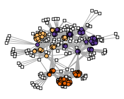
Figure 4: Feature–sample network for Iris dataset with all possible 128 and-features (excluding those with no connections). Circles are vertices associated with samples and squares with features. Colors represent the classes.

The optimal enhanced feature–sample network for this dataset is in Figure 4.

IV-A2 Community detection

Applying a greedy community detection method [16] in both networks, we observe that the enhanced network has modularity $12.4\%$ ($Q=0.561$) higher than the input network ($Q=0.499$.)

The enhanced network can also improve clustering tasks. If comparing the expected class and the obtained communities, the enhanced version achieves higher Jaccard index, $0.731$ against $0.719$.

IV-B Performance enhancement in supervised learning

Table I: UCI datasets along with the number of samples $N$, features $D$, and possible and-feature $M$.

Dataset	N	D	M
Breast 2010	106	27	134,217,700
Ecoli	336	19	524,268
Glass	214	25	33,554,406
Wine	178	39	549,755,813,848

We also apply our proposal in 4 classification tasks from UCI [15]. Section IV-B presents the datasets along with the number of samples $N$, features $D$, and possible and-features $M$. We highlight that it is unfeasible to list every possible combination among the features even for small datasets. The networks are generated as shown in [8] with $3$ bins.

The optimization process is executed $15$ times for each strategy – SPEA2 and GA. We fix the population size in $1000$, the archive size in $100$, and the elitism $100$ solutions. For the initial population, we use $\mu=50$ and $\sigma=10$. The recombination rate is $0.6$ and $\eta=1$ mutations are performed for each candidate solution. We limit the number of and-feature by $M_{max}=100D$. The execution is stopped after the 1000th generation.

Table II: Number of and-features and disproportion obtained by the optimization process for both strategies. Average and standard deviation are shown for each measurement.

Section IV-B summarizes the number of and-features and disproportion obtained by the optimization process. For the lexicographic GA, we show the average and the standard deviation of the measurements among the $100$ best individuals. For SPEA2, only the non-dominated solutions are considered.

As expected by considering the previous study (Section IV-A,) the lexicographic GA achieved better count of and-features – the maximum allowed –, but worse values of disproportion. The candidate solutions of SPEA2 present wide variation, but consistent lower disproportion.

Table III: Number of and-features, disproportion, and strategy of the results with lowest disproportion and highest number of and-features.

Dataset	Lowest disproportion	Highest number of and-features
Breast 2010	513, 0.000 (SPEA2)	2700, 0.129 (LGA)
Ecoli	166, 0.011 (SPEA2)	1900, 0.114 (LGA)
Glass	416, 0.019 (SPEA2)	2500, 0.130 (LGA)
Wine	413, 0.015 (SPEA2)	3900, 0.226 (LGA)

Table IV: Accuracy of the $k$-NN method on the UCI datasets using three different input networks – original, lowest disproportion, and highest number of and-features. For each setting, the best value of $k$ is shown.

Breast 2010 $0.65\pm 0.11$ (5) $0.62\pm 0.10$ (4) $\mathbf{0.66\pm 0.10}$ (3) Ecoli $0.77\pm 0.03$ (6) $\mathbf{0.78\pm 0.04}$ (4) $\mathbf{0.78\pm 0.04}$ (13) Glass $0.66\pm 0.07$ (7) $0.69\pm 0.06$ (6) $\mathbf{0.72\pm 0.07}$ (9) Wine $0.93\pm 0.05$ (19) $\mathbf{0.94\pm 0.05}$ (3) $\mathbf{0.94\pm 0.03}$ (3)

For each one of the datasets, we take the candidate solution with highest count of and-features and with the lowest disproportion among every solution produced. (We ignored a few solutions with less than 100 and-features.) Such candidate solutions, and the strategy that has found them, are indicated in Table III.

We solve the classification problems for each one of the datasets using the $k$-nearest neighbors method. As inputs we use the interaction matrices $\left(x_{ij}\in\{0,1\}\right)_{ij}$ of the original network and the enhance ones from the selected candidate solutions. We performed $20$ split validations with $70$ and $80\%$ of labeled samples for each case. We also varied $k\in\{1,2,\dots,20\}$.

The best results for each configuration are shown in Section IV-B. Improvements are highlighted in bold. Using the solution with the highest number of and-features, we improved the classification results in all cases. Using less and-features but with lower disproportion, we see improvements almost as good as using higher and-feature count.

V Conclusion

In this paper, we presented an unsupervised feature learning mechanism that works on datasets with binary features. First, the dataset is mapped into a feature–sample network. Then, a multi-objective optimization process selects a set of new vertices that correspond to new features to produce an enhanced version of the network.

We show that the enhanced network contains more information and can be exploited to improve the performance of machine learning methods.

To solve the optimization problem, we opted to design population-based metaheuristics. We used both a lexicographic GA and the SPEA2 algorithm to find the candidate solutions.

From the experiments, we conclude that the GA produces more new features in fewer generations. However, candidate solutions in SPEA2, besides having less new features, also improved the performance of machine learning methods.

This fact suggests that the disproportion is a good measurement of the quality of the selected set of and-features. In future works, we will correlate improvement and disproportion of the solutions with the same number of features.

Furthermore, the learning techniques used – fast-greedy community detection and $k$-nearest neighbors – do not take full advantage of the new features. In subsequent studies, we will elaborate learning models to exploit the enhanced feature–sample network explicitly.

Acknowledgments

This research was supported by the São Paulo State Research Foundation (FAPESP) and the Brazilian National Research Council (CNPq).

References

- [1] C. M. Bishop, Pattern Recognition and Machine Learning. Springer-Verlag New York, 2006.
- [2] X. Zhu and A. B. Goldberg, “Introduction to Semi-Supervised Learning,” Synthesis Lectures on Artificial Intelligence and Machine Learning, vol. 3, no. 1, pp. 1–130, 2009.
- [3] T. M. Cover, “Geometrical and statistical properties of systems of linear inequalities with applications in pattern recognition,” IEEE Transactions on Electronic Computers, vol. EC-14, no. 3, pp. 326–334, 1965.
- [4] T. C. Silva, L. Zhao, and T. H. Cupertino, “Handwritten data clustering using agents competition in networks,” Journal of Mathematical Imaging and Vision, vol. 45, no. 3, pp. 264–276, 2013.
- [5] T. C. Silva and L. Zhao, Machine Learning in Complex Networks, 1st ed. Springer, 2016.
- [6] F. A. N. Verri, P. R. Urio, and L. Zhao, “Network unfolding map by vertex-edge dynamics modeling,” IEEE Transactions on Neural Networks and Learning Systems, vol. PP, no. 99, pp. 1–14, 2016.
- [7] M. E. J. Newman, Networks: An Introduction, 1st ed. New York, NY: Oxford University Press, 2010.
- [8] F. A. N. Verri and L. Zhao, “Random walk in feature-sample networks for semi-supervised classification,” in 2016 5th Brazilian Conference on Intelligent Systems (BRACIS), 2016, pp. 235–240.
- [9] J. Mũnoz Marí, F. Bovolo, L. Gómez-Chova, L. Bruzzone, and G. Camp-Valls, “Semisupervised One-Class Support Vector Machines for Classification of Remote Sensing Data,” IEEE Trans. Geosci. Remote Sens., vol. 48, no. 8, pp. 3188–3197, 2010.
- [10] Y. Bengio, A. Courville, and P. Vincent, “Representation learning: A review and new perspectives,” IEEE Transactions on Pattern Analysis and Machine Intelligence, vol. 35, no. 8, pp. 1798–1828, 2013.
- [11] A. A. Freitas, “A critical review of multi-objective optimization in data mining: A position paper,” SIGKDD Explor. Newsl., vol. 6, no. 2, pp. 77–86, 2004.
- [12] E. Zitzler, M. Laumanns, and L. Thiele, “SPEA2: Improving the strength pareto evolutionary algorithm for multiobjective optimization,” in Evolutionary Methods for Design Optimization and Control with Applications to Industrial Problems. Athens, Greece: International Center for Numerical Methods in Engineering, 2001, pp. 95–100.
- [13] M. Srinivas and L. M. Patnaik, “Genetic algorithms: a survey,” Computer, vol. 27, no. 6, pp. 17–26, 1994.
- [14] C. A. Coello Coello, D. A. Van Veldhuizen, and G. B. Lamont, Evolutionary Algorithms for Solving Multi-Objective Problems. Secaucus, NJ, USA: Springer-Verlag New York, Inc., 2002.
- [15] M. Lichman, “UCI machine learning repository,” 2013. [Online]. Available: http://archive.ics.uci.edu/ml
- [16] A. Clauset, M. E. J. Newman, and C. Moore, “Finding community structure in very large networks,” Physical Review E, vol. 70, no. 6, pp. 1–6, 2004.