Iterative Machine Learning for Precision Trajectory Tracking with Series Elastic Actuators

Abstract

When robots operate in unknown environments small errors in postions can lead to large variations in the contact forces, especially with typical high-impedance designs. This can potentially damage the surroundings and/or the robot. Series elastic actuators (SEAs) are a popular way to reduce the output impedance of a robotic arm to improve control authority over the force exerted on the environment. However this increased control over forces with lower impedance comes at the cost of lower positioning precision and bandwidth. This article examines the use of an iteratively-learned feedforward command to improve position tracking when using SEAs. Over each iteration, the output responses of the system to the quantized inputs are used to estimate a linearized local system models. These estimated models are obtained using a complex-valued Gaussian Process Regression (cGPR) technique and then, used to generate a new feedforward input command based on the previous iteration’s error. This article illustrates this iterative machine learning (IML) technique for a two degree of freedom (2-DOF) robotic arm, and demonstrates successful convergence of the IML approach to reduce the tracking error.

I Introduction

Robots are now operated in unstructured environments where good control over the applied force is needed, especially if the robot needs to interact with humans or is operating in environments where large forces can lead to damage. Fine robot positioning with high bandwidth has been achieved traditionally using high impedance (i.e., very stiff) designs. However, such high impedance leads to poor force control due to large errors in force with small position deviations [1]. An increasingly popular solution for improved force control is the use of series elastic actuators (SEAs), which were introduced by Pratt and Williamson [1], with further control analysis done by Robinson [2]. SEAs introduce an elastic element in series between the motor and its load to lower output impedance. Additionally, the output force can be directly estimated by measuring the deformation of the elastic element [1], which can be used in safety-critical application, e.g., to stop the robot action if the forces are excessive. The original elastic actuator concept has inspired many other designs and their use in human-robot interaction applications, such as rehabilitation [3, 4, 5]. While adequate force control is achieved with SEAs, this is at the cost of lower performance in terms of positioning precision and bandwidth, and distrubance rejection [6, 7] due to lowered impedance, friction nonlinearities, and backlash [8, 2]. Recent control methods attempt to remedy these problems by modeling the higher order system dynamics associated with the SEAs, active system identification, and disturbance estimation [9, 10, 11]. Nevertheless, feedback methods tend to have performance limitations due to the nonminimum-phase behavior with the elastic elements.

Model-based methods, such as inversion to find feedforward inputs to augment the feedback, can improve performance of robots with elastic joints, e.g., [12]. Moreover, the effects of modeling uncertainty can be corrected using Iterative Learning Control (ILC) approaches, which can improve the tracking performance for repeated tasks [13, 14, 15, 16, 17, 18, 19, 20]. Nevertheless, if the initial modeling errors are large, then the iterative approach could diverge [21]. This has motivated approaches that use the data obtained during the iteration process without an explicit model to improve convergence [22]. Additionally, kernel-based Gaussian process regression has been used to update the models using iteration data [23] and such iterative machine learning (IML) approaches have been experimentally evaluated in [24]. The extension of such IML methods for finding the feedforward input to improve the precision when using SEAs is investigated in this article.

A challenge with modeling multi-linked robotic systems is that the system dynamics are nonlinear. To develop iterative corrections, the trajectory tracking control approach in this article finds localized linear system representations of the nonlinear system. The input-output data is then used to derive locally (linearized) models. For sufficiently-slow changes in the trajectory, the localized models can be used to develop iterative input corrections. The local models are obtained in the frequency domain using using complex-valued Gaussian Process Regression (cGPR) for fitting the measured input-output data. An advantage of the cGPR approach is that it also provides potential uncertainties in the models, which can be used to design the gains in the iteration law to promote convergence. The iteration approach allows large changes in input updates in frequency regions where the model uncertaintly is small. No changes or small changes in the in the input updates are used if the predicted model uncertainty is large[25, 26, 27].

II Problem Formulation and Solution

This section introduces the iterative machine learning (IML) procedure, which has previously been applied to scalar linear time-invariant (LTI) systems [23, 24] and presents two extensions for applications to: (i) linear time-varying (LTV) systems and (ii) multiple-input multiple-output (MIMO) systems. The application to LTV systems also allows for control of control-affine nonlinear systems that can be approximated as LTV systems parameterized about the desired trajectory.

II-A Iterative machine learning for scalar LTI systems

Consider a scalar LTI system, where the input $u$ and output $y$ are related by the impulse response $g$ as

$$y(t)=(g\star u)(t),$$ (1)

where $\star$ denotes convolution in the time domain, or equivalently in frequency domain by

$$Y(\omega)=G(\omega)U(\omega),$$ (2)

where $Y(\omega)=\mathcal{F}(y(\cdot))$, $U(\omega)=\mathcal{F}(u(\cdot))$, and $\mathcal{F}$ denotes the Fourier transform. The tracking problem for this system is to find an input $u^{*}$ such that the system output $y$ is equal to the desired output $y_{d}$, i.e., $y(t)=y_{d}(t)$. In the iterative learning control method, the input signal is iteratively corrected; given a previous input $U_{k-1}(\omega)$ which resulted in an output $Y_{k-1}(\omega)$, the correction is

$$U_{k}(\omega)=U_{k-1}(\omega)+\rho(\omega)\hat{G}^{-1}(\omega)(Y_{d}(\omega)-Y_{k-1}(\omega)),$$ (3)

where $\hat{G}^{-1}$ is an estimate of the inverse of the transfer function $G$ and $\rho$ is the frequency-dependent iteration gain. It was shown in [14] that this sequence converges to the desired input $U^{*}(\omega)$ at frequency $\omega$ if and only if

$$|\Delta_{p}(\omega)|<\pi/2$$ (4)

$$0<\rho(\omega)<\frac{2\cos\Delta_{p}(\omega)}{\Delta_{m}(\omega)}$$ (5)

where $\Delta_{m}$ and $\Delta_{p}$ are the magnitude and phase of the modeling error given by

$$\frac{G^{-1}}{\hat{G}^{-1}}=\Delta_{m}e^{j\Delta_{p}}.$$ (6)

Data-based modeling approaches can improve the convergence of the iterative control by increasing the accuracy of the inverse system model $\hat{G}^{-1}(\omega)$ used in the iteration law in Eq. (3). In the scalar LTI case, estimates of the inverse system model can be computed in the frequency domain as [22]

$$\hat{G}^{-1}(\omega)=U(\omega)/Y(\omega).$$ (7)

When the data is noisy or unavailable at some frequencies, such model estimates can be improved by using the data to train a complex-valued Gaussian process regression (cGPR) model of the form

$$\hat{G}^{-1}(\omega)=f(\omega)+\epsilon,$$ (8)

where $f(\omega)$ is the underlying true function and $\epsilon$ is a Gaussian noise term. In the Gaussian process framework, function values $f(\omega_{1})$ and $f(\omega_{2})$ are assumed to be correlated according to a kernel function $\hat{k}(\omega_{1},\omega_{2})$ which measures the similarity of the inputs $\omega_{1}$ and $\omega_{2}$. Given measured data $\hat{G}^{-1}_{T}\in\mathbb{C}^{n}$ at frequencies $\Omega_{T}\in\mathbb{R}^{n}$, the resulting estimated mean $\mathbb{E}$ and variance $\mathbb{V}$ of the underlying function $f(\omega)$ are given by[28]

$$\mathbb{E}[f(\omega)] =K(\omega,\Omega_{T})K_{T}^{-1}\hat{G}^{-1}_{T}(\Omega_{T}),$$ (9)

$$\mathbb{V}[f(\omega)] =K(\omega,\omega)-K(\omega,\Omega_{T})K_{T}^{-1}K(\Omega_{T},\omega),$$ (10)

where $K(\Omega_{1},\Omega_{2})$ is the covariance matrix formed by evaluating the kernel $\hat{k}(\cdot,\cdot)$ on all pair of entries from $\Omega_{1}$ and $\Omega_{2}$ and $K_{T}=K(\Omega_{T},\Omega_{T})+\sigma_{\epsilon}^{2}I$ is the covariance matrix of the noisy training data.

II-B Extension to LTV case

When the system is nonlinear, a transfer function approach is not valid in general. In the following, the system is approximated using an LTI model at every time instant $t$, which can vary over time, i.e., Eq. 2 as

$$y(t) =(g_{t}\star u)(t)$$ (11)

$$g_{t} =h(t,p_{1}(t),p_{2}(t),\dots,p_{m}(t)).$$ (12)

where the local system transfer function $g_{t}$ can vary with time, as can the potentially time-varying parameters $p_{1},p_{2},\dots,p_{m}$, which are assumed to be known or estimated at all times.

II-B1 Input update

The updated input signal at iteration $k$ evaluated at a specific time $t_{j}$, $u_{k}(t_{j})$, can be written as in Eq. 3 with the model ${G}_{t_{j}}$, in the frequency domain as

$$U_{k}(\omega)=U_{k-1}(\omega)+\rho(\omega){G}_{t_{j}}^{-1}(\omega)E_{k-1}(\omega),$$ (13)

where $e_{k}(t)=y_{d}(t)-y_{k}(t)$ is the error at iteration $k$ and time $t$, which is equivalent to, in the time domain,

$$u_{k}(t_{j}) =u_{k-1}(t_{j})+(\rho\star g_{t_{j}}^{-1}\star e_{k-1})(t_{j}),$$ (14)

Note that updating the input at time instant $t_{j}$ using the convolution requires the error $e_{k}(t)$ at time instants $t$ before and after the time-instant $t_{j}$.

II-B2 Model for input update

In the Gaussian process framework, learning the parameterized model means the system is taken to have the form

$$\hat{G}^{-1}(\mathbf{x})=f(\mathbf{x})+\epsilon,$$ (15)

where $\mathbf{x}=[\omega,p_{1},p_{2},\dots,p_{m}]$ and the kernel function $\hat{k}(\mathbf{x}_{1},\mathbf{x}_{2})$ depends in some sense on the distance between points in $\mathbb{R}^{m+1}$. The training data in this case consists of sampled local transfer function estimates $\hat{G}^{-1}_{T}$, which are computed by windowing the time-domain data and applying the Fourier transform to each segment, the corresponding frequencies $\Omega_{T}$, and representative parameter values for each segment. Then the locally-linear inverse transfer function $\hat{G}^{-1}(\omega)$ can be computed for each set of parameters $p_{i}(t)$ and the iterative update in Eq. 14 can be applied. The input correction can be computed for each model in frequency domain and sampled to retrieve the time index of interest, resulting in the update law

$$u_{k}(t_{j})=u_{k-1}(t_{j})+\mathcal{F}^{-1}\left.\left(\rho\hat{G}^{-1}_{j}\mathcal{F}(y_{d}(t)-y_{k-1}(t))\right)\right|_{t=t_{j}}$$ (16)

where $\hat{G}^{-1}_{j}\equiv\hat{G}^{-1}(\omega,p_{1}(t_{j}),p_{2}(t_{j}),\dots,p_{m}(t_{j}))\in\mathbb{C}^{n}$ is the estimated model based on the parameters at time $t_{j}$ evaluated at all frequencies.

II-C Extension to multivariate systems

When the system has more than one input, i.e.

$$Y_{i}(\omega)=\sum_{j=1}^{p}G_{ij}(\omega)U_{j}(\omega),$$ (17)

the individual transfer functions $G_{i}$ cannot be directly estimated from the data as in Eq. 7. Experimentally it may be viable to sample each transfer function by holding all other inputs zero; however, it is preferable to develop a learning method that is valid for the general case.

II-C1 Weighted kernel for single input case

Consider the case when the number of inputs $p=1$ and samples of the input $U_{1}\in\mathbb{C}^{n}$ and corresponding output $Y_{1}\in\mathbb{C}^{n}$ are available at frequencies $\Omega\in\mathbb{R}^{n}$. Then, similar to Eq. 7, the transfer function can be estimated as a Gaussian process

$$\hat{G}_{11}(\omega)=f_{11}(\omega)+\epsilon$$ (18)

with a kernel function $\hat{k}_{11}(\omega_{r},\omega_{s})$ and noisy transfer function samples $\hat{G}_{11r}=Y_{1r}/U_{1r}$ at frequency $\omega_{r}$. Equivalently, multiplying by the known input $U_{1}(\omega)$, the transfer function $G_{11}$ can be estimated from

$$Y_{1}(\omega)=f^{\prime}_{1}(\omega,U_{1})+\epsilon=f_{11}(\omega)U_{1}(\omega)+\epsilon$$ (19)

where the factor of $U_{1}(\omega)$ on the noise term $\epsilon$ has been dropped since the noise can be considered as output noise rather than process noise. The covariance of the input-weighted kernel $f_{1}^{\prime}$ is given by

$$\hat{k}_{11}^{\prime}(\omega_{r},\omega_{s}|U_{1r},U_{1s}) =\operatorname{cov}(f^{\prime}_{1}(\omega_{r},U_{1r}),f_{1}^{\prime}(\omega_{s},U_{1s}))$$

$$=\mathbb{E}[f^{\prime}_{1}(\omega_{r},U_{1r})\overline{f}_{1}^{\prime}(\omega_{s},U_{1s})]$$

$$=\mathbb{E}[f_{11}(\omega_{r})U_{1r}(\overline{f}_{11}(\omega_{s})\overline{U}_{1s})]$$

$$=U_{1r}\mathbb{E}[f_{11}(\omega_{r})\overline{f}_{11}(\omega_{s})]\overline{U}_{1s}$$

$$=U_{1r}\hat{k}_{11}(\omega_{r},\omega_{s})\overline{U}_{1s}.$$ (20)

where the overbar denotes complex conjugation and with an equivalent result in the case that $f_{11}$ is not a zero-mean process. The matched subscripts on $\omega_{r}$ and $U_{1r}$ indicate that $U_{1r}$ is an entry of the overall data vector $U_{1}$ with corresponding frequency $\omega_{r}$ from the data vector $\Omega$.

Remark 1 (Construction of covariance matrix)

The input-weighted kernel $\hat{k}_{11}^{\prime}$ in Eq. 20 gives rise to a covariance matrix of the form

$$K^{\prime}_{11}(\Omega,\Omega|U_{1},U_{1})=\mathrm{diag}(U_{1})K_{11}(\Omega,\Omega)\mathrm{diag}(\overline{U}_{1}),$$ (21)

where $K_{11}$ is the covariance matrix for the unweighted kernel $\hat{k}_{11}$. The input-weighted kernel $\hat{k}^{\prime}_{11}$ is a valid kernel if and only if the covariance matrix $K^{\prime}_{11}$ is positive semi-definite for any $\Omega$ and $U$, or, with the conjugate transpose denoted by superscript $H$,

$$0 \leq v^{H}K^{\prime}_{11}(\Omega,\Omega|U_{1},U_{1})v$$

$$=v^{H}\mathrm{diag}(U_{1})K_{11}(\Omega,\Omega)\mathrm{diag}(U_{1})^{H}v$$

$$=(\mathrm{diag}(U_{1})^{H}v)^{H}K_{11}(\Omega,\Omega)(\mathrm{diag}(U_{1})^{H}v)$$

$$=w^{H}K_{11}(\Omega,\Omega)w$$

which is satisfied for any valid unweighted kernel $\hat{k}_{11}$.

Remark 2 (Equivalence of weighted kernel)

Given measured frequency-domain input and output data $U_{1}$ and $Y_{1}$ at corresponding frequencies $\Omega$, the predictive mean at test frequencies $\Omega_{*}$ from the unweighted kernel is given by Eq. 9 as

$$\mathbb{E}[f_{11}(\Omega_{*})]=K_{*}(K+C_{\epsilon})^{-1}\tilde{G},$$ (22)

where $K=K_{11}(\Omega,\Omega)$, $K_{*}=K_{11}(\Omega_{*},\Omega)$, $C_{\epsilon}$ is the noise covariance matrix, and the estimated transfer function samples $\tilde{G}_{11}$ are computed by entry-wise division of $Y$ by $U$, i.e. $Y_{1}=\mathrm{diag}(U_{1})\tilde{G}_{11}$. Similarly, when using the input-weighted kernel $\hat{k}^{\prime}_{11}$ with test inputs $U_{1*}$ at corresponding frequencies $\Omega_{*}$, with $D\equiv\mathrm{diag}(U_{1})$ and $D_{*}\equiv\mathrm{diag}(U_{1*})$, and treating the noise as process noise with $C^{\prime}_{\epsilon}=DC_{\epsilon}\overline{D}$, the predictive mean is given by

$$\mathbb{E}[f^{\prime}_{11}(\Omega_{*},U_{*})] =K^{\prime}_{*}(K^{\prime}+C^{\prime}_{\epsilon})^{-1}Y_{1}$$

$$=D_{*}K_{*}\overline{D}(D(K+C_{\epsilon})\overline{D})^{-1}D\tilde{G}_{11}$$

$$=D_{*}K_{*}(K+C_{\epsilon})^{-1}\tilde{G}_{11}$$

$$=D_{*}\mathbb{E}[f_{11}(\Omega_{*})]$$ (23)

so by selecting $D_{*}=I$, an estimate of the transfer function $G$ is obtained that is equivalent to the estimate from the unweighted kernel $\hat{k}_{11}$.

II-C2 Generalization to multiple input case

In the case where the number of inputs $p$ is greater than 1, each transfer function $G_{ij}$ can be modeled as an independent Gaussian process with kernel $\hat{k}_{ij}$, resulting in a Gaussian process model for $Y_{i}$ as

$$Y_{i}(\omega) =f_{i}^{\prime}(\omega,U_{1},\dots,U_{p})=\sum_{j=1}^{p}f_{ij}(\omega)U_{j}(\omega)+\epsilon$$ (24)

and the weighted kernel function $\hat{k}^{\prime}_{i}$ can be derived using the identity that for independent random vectors $X$, $Y$,

$$\operatorname{cov}(X+Y,X+Y)=\operatorname{cov}(X,X)+\operatorname{cov}(Y,Y),$$ (25)

resulting in

$$\hat{k}^{\prime}_{i}(\omega_{r},\omega_{s}|\{U_{jr},U_{js}\}_{j=1}^{p})=\sum_{j=1}^{p}U_{jr}\hat{k}_{ij}(\omega_{r},\omega_{s})\overline{U}_{js}$$ (26)

and the corresponding covariance matrix

$$K^{\prime}_{i}=\sum_{j=1}^{p}\mathrm{diag}(U_{j})K_{ij}\mathrm{diag}(\overline{U}_{j}).$$ (27)

Then an estimate of an individual transfer function $\hat{G}_{ij}$ can be obtained by generating a Gaussian process prediction with $U_{j*}=\mathbf{1}$ and all other inputs identically zero. In the multiple-output case, Eq. 26 represents the kernel for estimating one line of the transfer matrix, i.e. each output corresponds to a multiple-input Gaussian process model with a kernel as in Eq. 26.

II-C3 Convergence conditions

In the case of square MIMO systems, conditions for local convergence are given by the following lemmas.

Lemma 1

For a fixed transfer matrix $G(\omega)\in\mathbb{C}^{N\times N}$, where $N$ is a positive integer, the sequence in Eq. 3 converges to $U^{*}(\omega)\in\mathbb{C}^{N}$ at frequency $\omega$ if and only if all eigenvalues of $(I-\rho(\omega)\hat{G}^{-1}(\omega)G(\omega))$ have magnitude less than one.

Proof:

From Eq. 3,

$$U_{k+1}-U_{k}=U_{k}+\rho\hat{G}^{-1}(Y_{d}-Y_{k})\\ -U_{k-1}-\rho\hat{G}^{-1}(Y_{d}-Y_{k-1}),$$ (28)

where the argument $\omega$ has been dropped for clarity. Then, cancelling the repeated factors of $Y_{d}$ and using the definition of the transfer matrix $G$,

$$U_{k+1}-U_{k} =U_{k}-U_{k-1}-\rho\hat{G}^{-1}G(U_{k}-U_{k-1})$$ (29)

$$=(I-\rho\hat{G}^{-1}G)(U_{k}-U_{k-1})$$ (30)

$$=(I-\rho\hat{G}^{-1}G)^{k}(U_{1}-U_{0}).$$ (31)

The sequence $U_{k}$ converges as $k\rightarrow\infty$ if and only if

$$\lim_{k\rightarrow\infty}(I-\rho\hat{G}^{-1}G)^{k}=0,$$ (32)

or, equivalently, if all eigenvalues of $(I-\rho\hat{G}^{-1}G)$ have magnitude less than one. ∎

Lemma 2 (Convergence for square MIMO systems)

Let $G(\omega)\in\mathbb{C}^{N\times N}$ be the fixed transfer matrix of a system with $N$ inputs and $N$ outputs evaluated at frequency $\omega$ and let $\hat{G}^{-1}(\omega)$ be an estimate of its inverse. Let the modeling error be described as $\Delta(\omega)\equiv\hat{G}^{-1}G$, with

$$[\Delta]_{ij}=\Delta_{mij}e^{j\Delta_{pij}}$$ (33)

where the diagonal terms are nonzero, i.e., $\Delta_{mii}\neq 0$ for all $i$. Then the sequence

$$U_{k}(\omega)=U_{k-1}(\omega)+\rho(\omega)\hat{G}^{-1}(\omega)(Y_{d}(\omega)-Y_{k-1}(\omega))$$ (34)

converges to the desired input $U^{*}(\omega)$ at frequency $\omega$ if the iteration gain $\rho(\omega)=\mathrm{diag}(\rho_{1}(\omega),\dots,\rho_{N}(\omega))$ satisfies the conditions

$$0<\rho_{i}(\omega) <2\frac{\Delta_{mii}\cos\Delta_{pii}-\sum_{j\neq i}\Delta_{mij}}{\Delta_{mii}^{2}-\left(\sum_{j\neq i}\Delta_{mij}\right)^{2}}$$ (35)

$$\Delta_{mii}\cos\Delta_{pii} >\sum_{j\neq i}\Delta_{mij}$$ (36)

where the subscript $j$ is an index and not $\sqrt{-1}$.

Proof:

By Lemma 1, proving convergence amounts to proving the magnitudes of the eigenvalues of $(I-\rho\hat{G}^{-1}G)$ are less than 1. By the Gershgorin disc theorem, the eigenvalues lie in the union of the discs with centers $C_{i}=1-\rho_{i}\Delta_{ii}$ and radii $R_{i}=\sum_{j\neq i}|\rho_{i}\Delta_{ij}|=\rho_{i}\sum_{j\neq i}\Delta_{mij}$ for $i\leq N$. The maximum distance from the origin to a point in disc $i$ is then given by $|C_{i}|+R_{i}$, so disc $i$ is bounded by the unit circle if and only if

$$1>{} |1-\rho_{i}\Delta_{ii}|+R_{i}$$ (37)

$$1-R_{i}>{} |1-\rho_{i}\Delta_{mii}(\cos\Delta_{pii}+j\sin\Delta_{pii})|.$$

If the above statement is true, then $(1-R_{i})\geq 0$ and therefore, the square must also hold, i.e.,

$$(1-R_{i})^{2}>{} (1-\rho_{i}\Delta_{mii}\cos\Delta_{pii})^{2}+\rho_{i}^{2}\Delta_{mii}^{2}\sin^{2}\Delta_{pii}$$

$$1-2R_{i}+R_{i}^{2}>{} 1+\rho_{i}^{2}\Delta_{mii}^{2}-2\rho_{i}\Delta_{mii}\cos\Delta_{pii}.$$

Finally, after cancelling the like terms and dividing by the positive gain $\rho_{i}$, this expression can be rearranged as

$$\rho_{i}[\Delta_{mii}^{2}-(\sum_{j\neq i}\Delta_{mij})^{2}]<{} 2(\Delta_{mii}\cos\Delta_{pii}-\sum_{j\neq i}\Delta_{mij}).$$ (38)

Since $\Delta_{mii}\neq 0$, the condition in Eq. 36 implies that

$$\cos\Delta_{pii}>0.$$

Moreover, since $\cos\Delta_{pii}$ is less than one, from the condition in Eq. 36,

$$\Delta_{mii}>\sum_{j\neq i}\Delta_{mij}\geq 0,$$ (39)

and squaring the uncertainties on both sides yields

$$\Delta_{mii}^{2}-(\sum_{j\neq i}\Delta_{mij})^{2}>0,$$ (40)

which leads to Eq. 35 from Eq. 38. The use of the phase condition in Eq. 36, rather than a condition as in Eq. 39, ensures that the right hand side of Eq. 35 is nonzero, which allows the selection of a nonzero iteration gain $\rho_{i}$.

∎

Remark 3 (Specialization to scalar case)

When the dimension of the transfer matrix $N=1$, or when the error in the off-diagonal terms is zero, Eqs. 35 and 36 are equivalent to the expressions given for scalar systems in Eqs. 4 and 5.

Lemma 3 (Convergence with bounded uncertainty)

When the errors in the real and imaginary components of the estimated model $\hat{G}$ are bounded as

$$|\hat{a}_{ij}-a_{ij}|\leq\Delta_{aij}$$ (41)

$$|\hat{b}_{ij}-b_{ij}|\leq\Delta_{bij}$$ (42)

with

$$G_{ij} =a_{ij}+jb_{ij},$$ (43)

$$\hat{G}_{ij} =\hat{a}_{ij}+j\hat{b}_{ij},$$ (44)

the condition in Eq. 35 is satisfied if

$$0<\rho_{i}<2\frac{1-\operatorname{Re}\hat{r}_{abs,i}\Delta_{ai}-\operatorname{Im}\hat{r}_{abs,i}\Delta_{bi}-|\hat{r}_{i}|D_{i}}{|\hat{r}_{i}|^{2}|\hat{c}_{abs,i}+\Delta_{ai}+j\Delta_{bi}|^{2}}$$ (45)

where $\hat{r}_{i}$ is the $i$th row of the inverse transfer matrix $\hat{G}^{-1}$, $\hat{c}_{i}$ is the $i$th column of the forward transfer matrix $\hat{G}$, $\Delta_{ai}$ and $\Delta_{bi}$ denote the $i$th column of the real and imaginary uncertainty matrices $\Delta_{a}$ and $\Delta_{b}$ defined in Eq. 41, Eq. 42,

$$[\hat{c}_{abs,i}]_{j} =|\operatorname{Re}\hat{c}_{ij}|+j|\operatorname{Im}\hat{c}_{ij}|,$$ (46)

$$D_{i} =\sum_{j\neq i}|\Delta_{aj}+j\Delta{bj}|,$$ (47)

$$[\operatorname{Re}\hat{r}_{abs,i}]_{j} =|\operatorname{Re}\hat{r}_{ij}|$$ (48)

$$[\operatorname{Im}\hat{r}_{abs,i}]_{j} =|\operatorname{Im}\hat{r}_{ij}|.$$ (49)

Proof:

The lemma amounts to finding a lower bound on the right-hand-side of Eq. 35 under the uncertainty $\Delta_{a}+j\Delta_{b}$. It is convenient to first develop bounds on the terms in the fraction. Note that $\Delta_{ij}=\hat{r}_{i}c_{j}$, where $c_{j}$ is the $j$th column of the forward transfer matrix $G$. Then the magnitude $\Delta_{mij}$ is

$$\Delta_{mij} =|\hat{r}_{i}c_{j}|=|\hat{r}_{i}(\hat{c}_{j}+e_{j})|=|\delta_{ij}+\hat{r}_{i}e_{j}|$$ (50)

where the real and imaginary parts of the error term $e_{j}$ is bounded by Eqs. 43 and 44. Then, using the Cauchy-Schwarz inequality, the magnitude can be bounded as

$$\Delta_{mij}\leq\begin{cases}|\hat{r}_{i}||\Delta_{aj}+j\Delta_{bj}|,&i\neq j\\ |\hat{r}_{i}||\hat{c}_{abs,i}+\Delta_{ai}+j\Delta_{bi}|,&i=j\end{cases}$$ (51)

where in the case of $i=j$ the second term is the maximum magnitude of $|\hat{c}_{i}|$ due to the bounds in Eqs. 43 and 44.

Similarly,

$$\Delta_{mii}\cos\Delta_{pii} =\operatorname{Re}(\hat{r}_{i}c_{i})=\operatorname{Re}(\delta_{ii}+\hat{r}_{i}e_{i})$$ (52)

$$=1+\operatorname{Re}(\hat{r}_{i})\operatorname{Re}(e_{i})-\operatorname{Im}(\hat{r}_{i})\operatorname{Im}(e_{i}),$$ (53)

which is minimized when every entry of $e_{i}$ has the same (maximum) magnitude as $\Delta_{ai}+j\Delta_{bi}$ and every term in the product is negative, resulting in

$$\Delta_{mii}\cos\Delta_{pii}\geq 1-\operatorname{Re}\hat{r}_{abs,i}\Delta_{ai}-\operatorname{Im}\hat{r}_{abs,i}\Delta_{bi}.$$ (54)

Combining these bounds on the terms in Eq. 35 leads to the expression in Eq. 45. ∎

Remark 4 (Local convergence of time-varying model)

In the preceding Lemmas 1, 2 and 3, the iteration-law was designed assuming a time-invariant system. For the time-varying case, as in Section II-B, the iteration law designed using the fixed model is anticipated to converge provided the time-variations are sufficiently slow. The convergence conditions for such variations could be developed using Picard-type arguments, e.g., as studied in [29] for the nonlinear case.

III Experiments

III-A Experimental system

The experimental system, used to evaluate the proposed IML approach, was a 2-DOF robotic arm, illustrated in Figures 1 and 2. The arm was constructed out of HEBI X5-4 series elastic actuators, black 1.25”$\oslash$ PVC Pipe, aluminum brackets, and a steel plate for mass, as shown in Figure 2. Each X5-4 actuator contains: a microcontroller, motor drive, Ethernet communication/daisy chain, encoder, series elastic element, and status LED. The X5-4 is capable of $4\text{\,}\mathrm{N}\text{\,}\mathrm{m}\text{/}$ continuous torque ($7\text{\,}\mathrm{N}\text{\,}\mathrm{m}\text{/}$ peak), 32 RPM max, $\pm$ 4 turn absolute encoder with 0.005^∘ resolution, and contains a torsional spring in series between motor and load with a stiffness of about $70\text{\,}\mathrm{N}\text{\,}\mathrm{m}\text{/}\mathrm{rad}$. Each actuator weighs approximately $340\text{\,}\mathrm{g}\text{/}$.

MATLAB was used to communicate over Ethernet with the X5’s on-board microcontrollers. Data was logged locally on each actuator, and subsequently retrieved and processed via MATLAB interface.

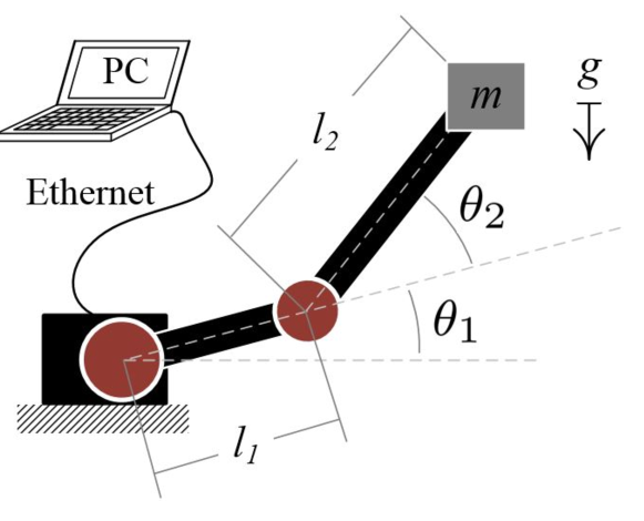
Figure 1: System diagram. 2-DOF Robotic Arm, driven angles $\theta_{1}$ and $\theta_{2}$, with link lengths of $l_{1}$ = 6.25” and $l_{2}$ = 10.5”, supporting a mass, $m$ = $275\text{\,}\mathrm{g}\text{/}$, at the end of link 2. Actuator communication to PC over Ethernet.

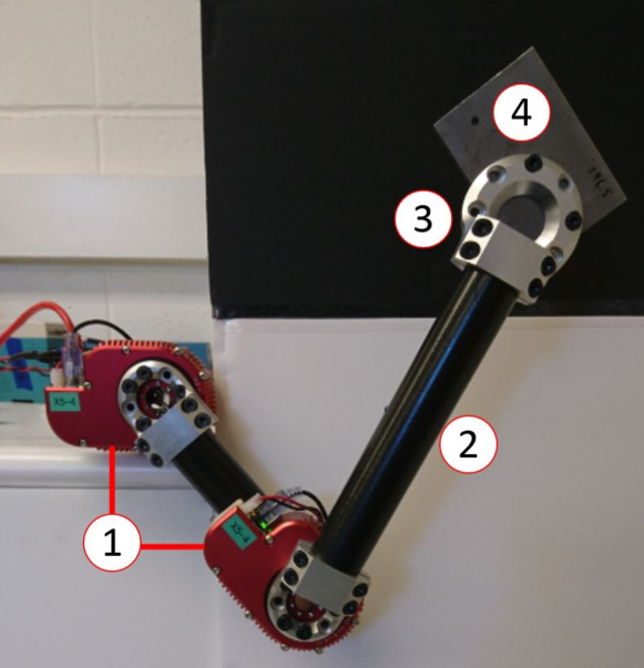
Figure 2: Experimental Setup. Robot arm consisting of: (1) HEBI X5-4 Series Elastic Actuators, (2) black 1.25”$\oslash$ PVC piping, and (3) aluminum brackets, supporting a (4) small steel plate.

III-B Application of iterative machine learning for joint control

To verify the ability to track trajectories with varying parameters, two trajectories were tested: i) a “slow” large-range-of-motion trajectory that moves both joints through an angle $\pi$, and ii) a “fast” short-range-of-motion trajectory that moves both joints through an angle $\pi/2$, both with a sinusoidal acceleration profile. Application of the iterative machine learning algorithm requires addressing the angle-dependent dynamics as presented in Section II-B with the joint angles $\theta_{1}(t)$ and $\theta_{2}(t)$ as the parameters. Additionally, there is coupling between the inputs. Each of the two inputs $u_{1}(t)$ and $u_{2}(t)$ have significant contribution to the response of both joint angles, so the multiple-input multiple-output case was considered as in Section II-C. The kernel function for each transfer function was selected as the squared-exponential kernel with automatic relevance determination [28],

$$\hat{k}_{ij}(\mathbf{x}_{1},\mathbf{x}_{2})=\sigma_{f}^{2}\exp\left(-\frac{1}{2}(\mathbf{x}_{1}-\mathbf{x}_{2})^{H}\Lambda(\mathbf{x}_{1}-\mathbf{x}_{2})\right)$$ (55)

where $\Lambda=\mathrm{diag}(\ell_{1}^{-2},\,\ell_{2}^{-2},\,\ell_{3}^{-2})$ is a matrix of length scales for the input variables $\mathbf{x}\equiv\begin{bmatrix}\omega&\theta_{1}&\theta_{2}\end{bmatrix}^{T}$ and the superscript $H$ denotes the complex conjugate transpose.

To improve the initial models, a quantized and slowed initial trajectory $u_{0}^{\prime}(t)$ was used, which is shown in Fig. 3. This method is similar to the augmented training signal used in [24], and helps ensure that sufficient frequency data is available by sampling the frequency response at discrete states along the desired trajectory.

When training the model, the parameters $\theta_{1}$ and $\theta_{2}$ were rounded to the nearest $\pi/10\approx$0.314\text{\,}\mathrm{rad}\text{/}$$ and frequency-response data was taken from a $2\text{\,}\mathrm{s}\text{/}$ window after each change in the discretized joint angles. After each iteration $k$, the resulting data were thresholded to include only the frequency components at which both the input and output magnitudes were at least 50% of the maximum magnitudes in the window, which selects the most relevant data and reduces the number of training points to save computational cost. The additional data from iteration $k$ was combined with the data from iterations $1$ through $k-1$ to obtain the training set. Then hyperparameters for each output kernel $\hat{k}^{\prime}_{i}$ were obtained by maximizing the marginal likelihood for the training data as described in [28]. After learning the hyperparameters, the model was estimated at each unique joint angle combination in $y_{k}(t)$, e.g. as in Figs. 15 and 16, and the correction in Eq. 16 was applied at all time points matching those parameters, resulting in an updated input signal $u_{k+1}(t)$. When computing the update, the iteration gains were computed as $60\%$ of the maximum given in Eq. 35 with the uncertainty bounds selected as

$$\Delta_{a}=\Delta_{b}=2\sqrt{\mathbb{V}[f(\omega)]}.$$ (56)

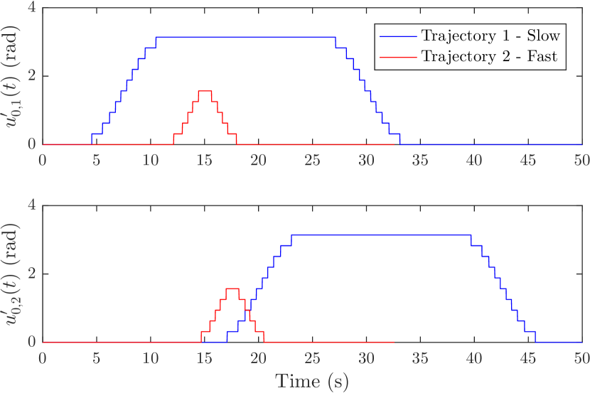
Figure 3: Augmented initial trajectory $u_{0}^{\prime}(t)$

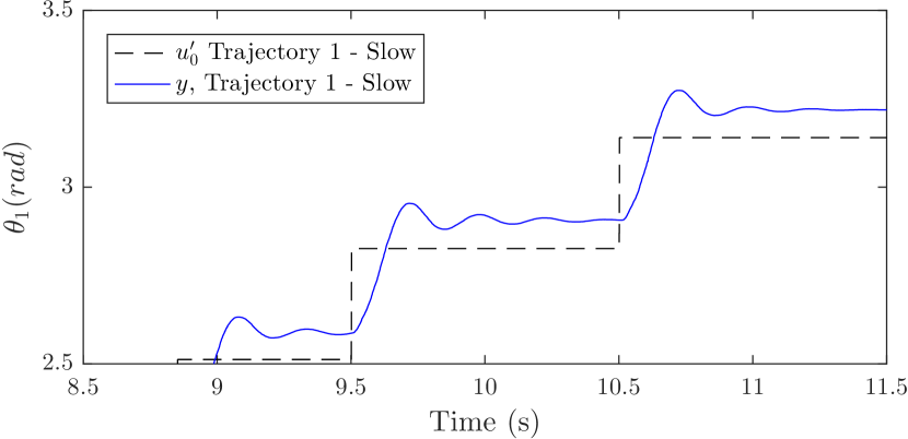
Figure 4: Step response of $\theta_{1}$ from the augmented initial trajectory 1, $u_{0}^{\prime}(t)$, shown in Fig. 3.

III-C Tracking results

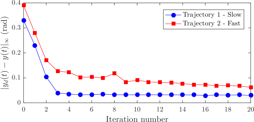
Figure 5: Convergence of the iterative machine learning procedure for the series-elastic robot arm.

The iterative gains derived in Eq. 35 and the multiple-input iterative machine learning procedure were successfully used to control the joint angles of the series elastic robot, as shown by the convergence behavior in Fig. 5, with a final full range of motion error of $0.029\text{\,}\mathrm{rad}\text{/}$ and $0.062\text{\,}\mathrm{rad}\text{/}$, or $1\text{\,}\mathrm{\char 37\relax}\text{/}$ and $4\text{\,}\mathrm{\char 37\relax}\text{/}$, for trajectories 1 and 2, respectively. This is a 91% and a 84% reduction in error for trajectories 1 and 2, respectively, compared to using the DC gain $G_{0}$ alone. Convergence was achieved after five iterations for the slow trajectory, suggesting that the bounds on the iteration gain were not overly restrictive. Convergence for the faster trajectory is slower and seems to continue past 20 iterations. Such slower convergence indicates larger modeling errors at the higher frequencies. Also, the time variations in the system, which are neglected in the modeling, can be more significant, which also impacts convergence. The initial error using $u_{0}(t)=y_{d}(t)/G_{0}$ and the error for the final learned input $u_{20}(t)$ are compared in Figs. 6 and 7 and the corresponding inputs are shown in Figs. 8 and 9. The maximum error values for trajectory 1 started at

$$\left[\max|\Delta\theta_{1}|,\max|\Delta\theta_{2}|\right]_{k=0}=[0.331,0.287]$\text{\,}\frac{\mathrm{rad}}{}$,$$

and reduced to

$$\left[\max|\Delta\theta_{1}|,\max|\Delta\theta_{2}|\right]_{k=20}=[0.029,0.029]$\text{\,}\frac{\mathrm{rad}}{}$.$$

Similarly, the maximum error values for trajectory 2 started at

$$\left[\max|\Delta\theta_{1}|,\max|\Delta\theta_{2}|\right]_{k=0}=[0.390,0.266]$\text{\,}\frac{\mathrm{rad}}{}$,$$

and reduced to

$$\left[\max|\Delta\theta_{1}|,\max|\Delta\theta_{2}|\right]_{k=20}=[0.062,0.044]$\text{\,}\frac{\mathrm{rad}}{}$.$$

These substantial error reductions between the initial and final output-trajectories, as shown in Figs. 10, 11, 12 and 13, confirm that the IML method can successfully learn the input to improve the tracking performance of the SEA robot.

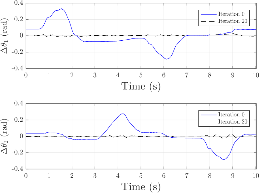
Figure 6: Trajectory 1. Comparison of the initial (—) and final (- - -) error signals on the two joint angles $\theta_{1}(t)$ and $\theta_{2}(t)$.

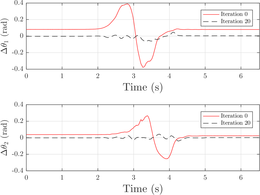
Figure 7: Trajectory 2. Comparison of the initial (—) and final (- - -) error signals on the two joint angles $\theta_{1}(t)$ and $\theta_{2}(t)$.

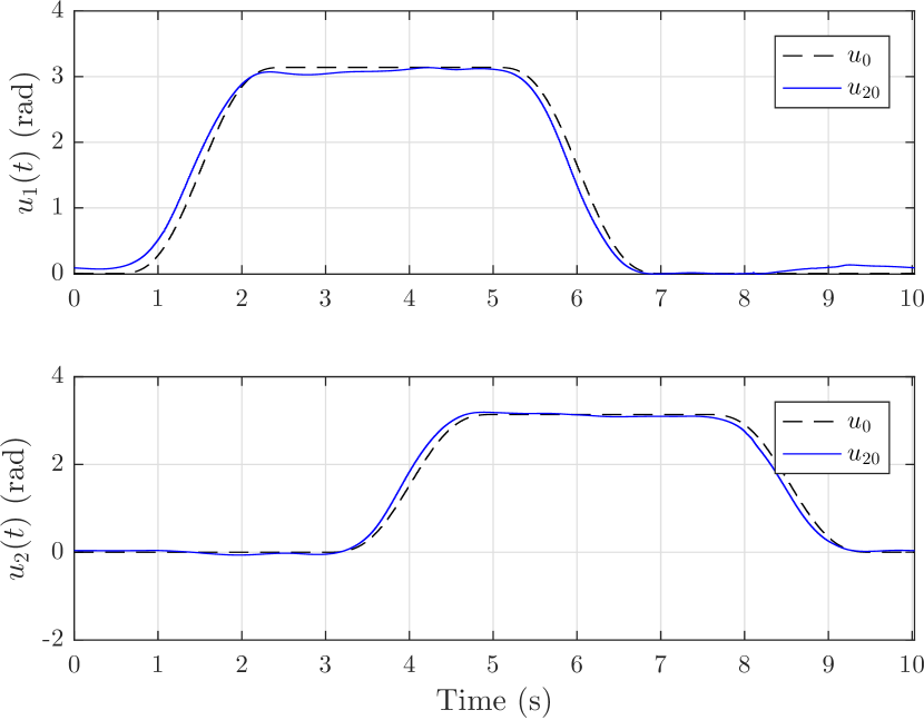
Figure 8: Trajectory 1. Comparison of the initial input $u_{0}(t)=y_{d}/G_{0}$ (- - -) and the final learned input $u_{20}(t)$ (—).

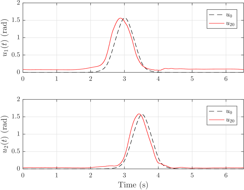
Figure 9: Trajectory 2. Comparison of the initial input $u_{0}(t)=y_{d}/G_{0}$ (- - -) and the final learned input $u_{20}(t)$ (—).

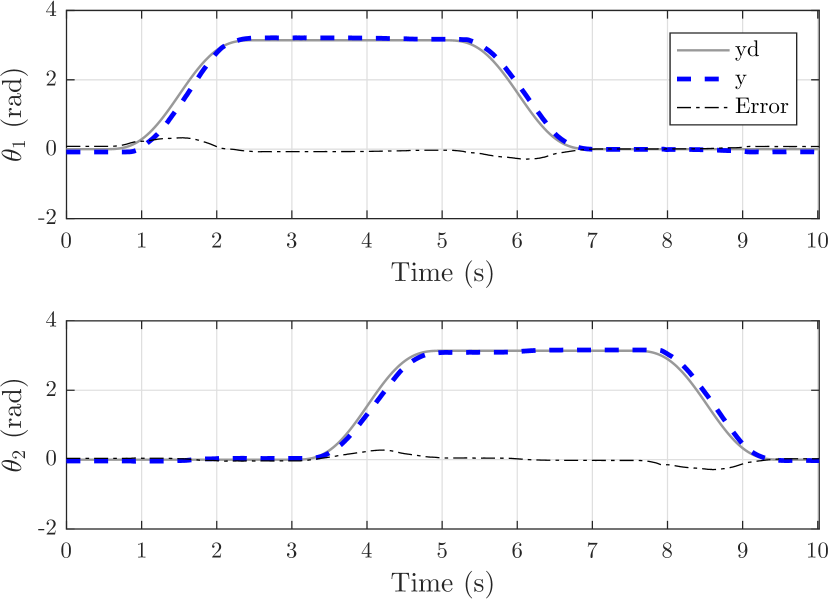
Figure 10: Output Tracking Trajectory 1. Iteration 0. Comparison of desired trajectory, $y_{d}$, achieved trajectory, $y$, and error between them.

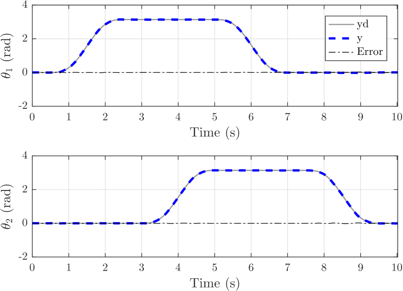
Figure 11: Output Tracking Trajectory 1. Iteration 20. Comparison of desired trajectory, $y_{d}$, achieved trajectory, $y$, and error between them.

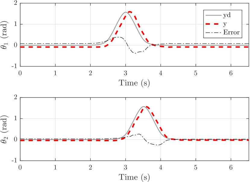
Figure 12: Output Tracking Trajectory 2. Iteration 0. Comparison of desired trajectory, $y_{d}$, achieved trajectory, $y$, and error between them.

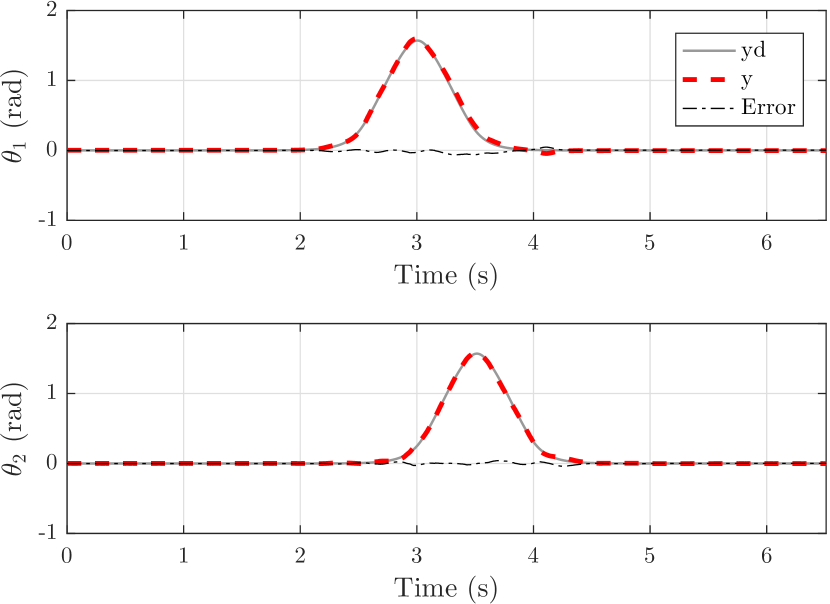
Figure 13: Output Tracking Trajectory 2. Iteration 20. Comparison of desired trajectory, $y_{d}$, achieved trajectory, $y$, and error between them.

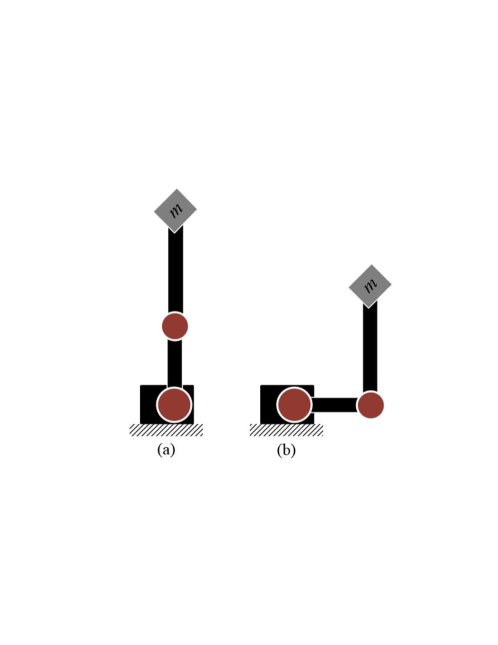
Figure 14: Robot poses used in generating the bode plots in Figs. 15 and 16. (a) $\theta_{1}$ = $\pi$/2, $\theta_{2}$ = 0 and (b) $\theta_{1}$ = 0, $\theta_{2}$ = $\pi$/2. See Fig. 1 for more details.

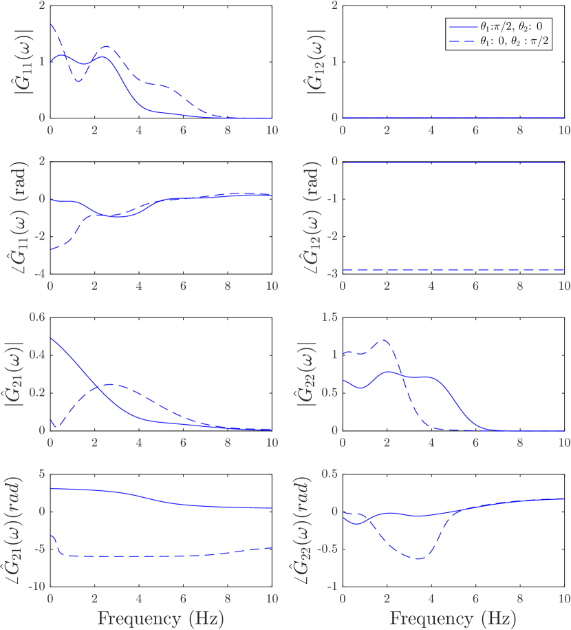
Figure 15: Trajectory 1. Linearized model estimates of the system after 20 iterations at two different poses (sets of $\theta_{1}$ and $\theta_{2}$ positions). See Fig. 14 for poses. The eight plots show magnitude and phase of the MIMO system – two inputs and two outputs.

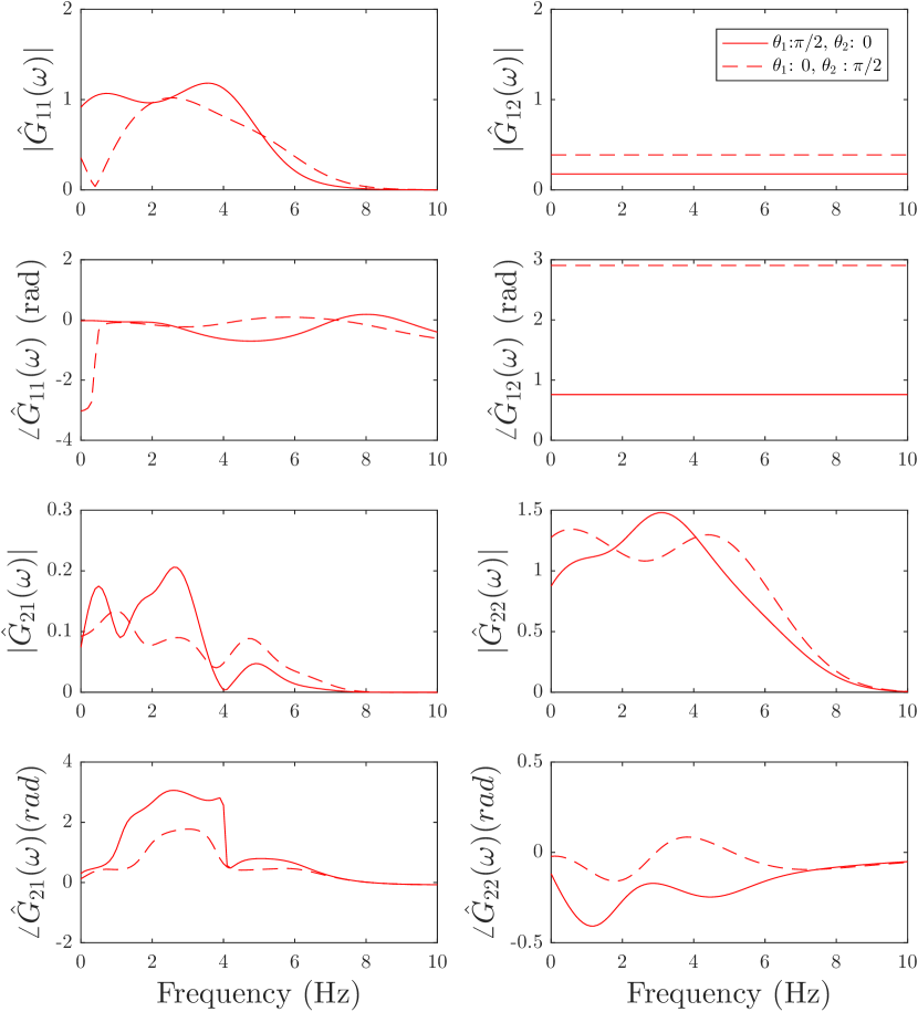
Figure 16: Trajectory 2. Linearized model estimates of the system after 20 iterations at two different poses (sets of $\theta_{1}$ and $\theta_{2}$ positions). See Fig. 14 for poses. The eight plots show magnitude and phase of the MIMO system – two inputs and two outputs.

IV Conclusions

An iterative machine learning (IML) method was proposed that enables iterative control of control-affine nonlinear multiple-input multiple-output systems with unknown dynamics. Conditions on local convergence were presented and the method was tested on a two-link robotic arm driven by series elastic actuators. The iterative machine learning approach converged to an input with a maximum error in the joint angles of 1% and 4% of the range of motion for trajectories 1 and 2, respectively. Current efforts are aimed at developing global conditions of the rate of acceptable trajectory variations to ensure convergence of the proposed iterative approach with the localized models.

References

- [1] G. A. Pratt and M. M. Williamson, “Series Elastic Actuators,” IEEE/RSJ International Conference on Intelligent Robots and Systems, pp. 399–406, 1995.
- [2] D. W. Robinson, “Design and Analysis of Series Elasticity in Closed-loop Actuator Force Control,” Ph.D. dissertation, Massachusetts Institute of Technology, Cambridge, MA, USA, 2000.
- [3] B. Kim, A. Rodot, and A. D. Deshpande, “Impedance Control Based on a Position Sensor in a Rehabilitation Robot,” ASME 2014 Dynamic Systems and Control Conference, no. 1, pp. 1–7, 2014.
- [4] U. Nagarajan, G. Aguirre-Ollinger, and A. Goswami, “Integral admittance shaping: A unified framework for active exoskeleton control,” Robotics and Autonomous Systems, vol. 75, Part B, pp. 310–324, 2016. [Online]. Available: http://www.sciencedirect.com/science/article/pii/S0921889015002031
- [5] X. Li, Y. Pan, G. Chen, and H. Yu, “Adaptive Human-Robot Interaction Control for Robots Driven by Series Elastic Actuators,” IEEE Transactions on Robotics, vol. 33, no. 1, pp. 1–14, 2016. [Online]. Available: http://ieeexplore.ieee.org/document/7782391/
- [6] N. Paine, S. Oh, and L. Sentis, “Design and control considerations for high-performance series elastic actuators,” IEEE/ASME Transactions on Mechatronics, vol. 19, no. 3, pp. 1080–1091, 2014.
- [7] V. Chawda and G. Niemeyer, “Toward controlling a KUKA LBR IIWA for interactive tracking,” IEEE International Conference on Robotics and Automation (ICRA), pp. 1808–1814, 2017.
- [8] S. D. Eppinger, “Modeling robot dynamic performance for endpoint force control,” PhD Thesis, Massachusetts Institute of Technology, 1988.
- [9] A. Muller and J. Kepler, “Recursive Second-Order Inverse Dynamics for Serial Manipulators,” IEEE International Conference on Robotics and Automation (ICRA), pp. 2483–2489, 2017.
- [10] E. Sariyildiz, H. Wang, and H. Yu, “A Sliding Mode Controller Design for the Robust Position Control Problem of Series Elastic Actuators,” IEEE International Conference on Robotics and Automation (ICRA), pp. 3055–3061, 2017.
- [11] X. Li, G. Chen, Y. Pan, and H. Yu, “Region control for robots driven by series elastic actuators,” IEEE International Conference on Robotics and Automation (ICRA), pp. 1102–1107, 2016.
- [12] A. De Luca and P. Lucibello, “A general algorithm for dynamic feedback linearization of robots with elastic joints,” in Proc. of the IEEE Intenational Conference on Robotics & Automation, Leuven, Belgium, May 1998, pp. 504–510.
- [13] A. J. McDaid, K. C. Aw, E. Haemmerle, and S. Q. Xie, “Control of IPMC actuators for microfluidics with adaptive “online” iterative feedback tuning,” IEEE/ASME Transactions on Mechatronics, vol. 17, no. 4, pp. 789–797, aug 2012. [Online]. Available: https://doi.org/10.1109/tmech.2011.2135373
- [14] S. Tien, Q. Zou, and S. Devasia, “Iterative control of dynamics-coupling-caused errors in piezoscanners during high-speed afm operation,” IEEE Transactions on Control Systems Technology, vol. 13, no. 6, pp. 921–931, 2005.
- [15] M. Butcher and a. Karimi, “Linear Parameter-Varying Iterative Learning Control With Application to a Linear Motor System,” IEEE/ASME Transactions on Mechatronics, vol. 15, no. 3, pp. 412–420, 2010.
- [16] J. Ghosh and B. Paden, “Nonlinear repetitive control,” IEEE Transactions on Automatic Control, vol. 45(5), pp. 949–954, 2000.
- [17] M.-S. Tsai, C.-L. Yen, and H.-T. Yau, “Integration of an Empirical Mode Decomposition Algorithm With Iterative Learning Control for High-Precision Machining,” Mechatronics, IEEE/ASME Transactions on, vol. 18, no. 3, pp. 878–886, 2013.
- [18] S. Mishra and M. Tomizuka, “Projection-based iterative learning control for wafer scanner systems,” IEEE/ASME Transactions on Mechatronics, vol. 14, no. 3, pp. 388–393, 2009.
- [19] H. Havlicsek and A. Alleyne, “Nonlinear control of an electrohydraulic injection molding machine via iterative adaptive learning,” IEEE/ASME Transactions on Mechatronics, vol. 4, no. 3, pp. 312–323, 1999.
- [20] C. Atkeson and J. McIntyre, “Robot trajectory learning through practice,” in Robotics and Automation. Proceedings. 1986 IEEE International Conference on, vol. 3. IEEE, 1986, pp. 1737–1742.
- [21] H. Ahn, Y. Q. Chen, and K. L. Moore, “Iterative learning control: Brief survey and categorization,” IEEE Transactions on Systems, Man, and Cybernetics, Part C: Applications and Reviews, vol. 37(6), pp. 1099–1121, 2007.
- [22] K.-S. Kim and Q. Zou, “Model-less inversion-based iterative control for output tracking: Piezo actuator example,” Proceedings of American Control Conference, Seattle, WA, pp. 2170–2715, June 11-13, 2008.
- [23] S. Devasia, “Iterative machine learning for output tracking,” submitted to IEEE Transactions on Control Systems Technology, 2017, Online available at https://arxiv.org/pdf/1705.07826v2.pdf.
- [24] N. Banka and S. Devasia, “Iterative machine learning for output tracking with magnetic soft actuators,” in review.
- [25] L. Blanken, F. Boeren, D. Bruijnen, and T. Oomen, “Batch-to-Batch Rational Feedforward Control: From Iterative Learning to Identification Approaches, With Application to a Wafer Stage,” IEEE-ASME TRANSACTIONS ON MECHATRONICS, vol. 22, no. 2, pp. 826–837, APR 2017.
- [26] Y. Liu and Y. Zhang, “Iterative Local ANFIS-Based Human Welder Intelligence Modeling and Control in Pipe GTAW Process: A Data-Driven Approach,” IEEE-ASME TRANSACTIONS ON MECHATRONICS, vol. 20, no. 3, pp. 1079–1088, JUN 2015.
- [27] M. Norrlof, “An adaptive iterative learning control algorithm with experiments on an industrial robot,” IEEE Transactions on Robotics and Automation, vol. 18, no. 2, pp. 245–251, Apr 2002.
- [28] C. E. Rasmussen and C. K. I. Williams, Gaussian Processes for Machine Learning. Cambridge, MA: The MIT Press, 2006.
- [29] B. Altın and K. Barton, “Exponential stability of nonlinear differential repetitive processes with applications to iterative learning control,” Automatica, vol. 81, pp. 369–376, 2017.