How to get high resolution results from sparse and coarsely sampled data

Abstract

Sampling a signal below the Shannon-Nyquist rate causes aliasing, meaning different frequencies to become indistinguishable. It is also well-known that recovering spectral information from a signal using a parametric method can be ill-posed or ill-conditioned and therefore should be done with caution.

We present an exponential analysis method to retrieve high-resolution information from coarse-scale measurements, using uniform downsampling. We exploit rather than avoid aliasing. While we loose the unicity of the solution by the downsampling, it allows to recondition the problem statement and increase the resolution.

Our technique can be combined with different existing implementations of multi-exponential analysis (matrix pencil, MUSIC, ESPRIT, APM, generalized overdetermined eigenvalue solver, simultaneous QR factorization, $\ldots$) and so is very versatile. It seems to be especially useful in the presence of clusters of frequencies that are difficult to distinguish from one another.

Keywords: Exponential analysis, parametric method, Prony’s method, sub-Nyquist sampling, uniform sampling, sparse interpolation, signal processing.

Mathematics Subject Classication (2010): 42A15, 65Z05, 65T40.

1 Introduction

Estimating the fine scale spectral information of an exponential sum plays an important role in many signal processing applications. The problem of superresolution [1, 2] has therefore recently received considerable attention.

Despite its computational efficiency and wide applicability, the often used Fourier transform (FT) has some well-known limitations, such as its limited resolution and the leakage in the frequency domain. These restrictions complicate the analysis of signals falling exponentially with time. Fourier analysis, which represents a signal as a sum of periodic functions, is not very well suited for the decomposition of aperiodic signals, such as exponentially decaying ones. The damping causes a broadening of the spectral peaks, which in its turn leads to the peaks overlapping and masking the smaller amplitude peaks. The latter are important for the fine level signal classification.

Signals that fall exponentially with time appear, for instance, in transient detection, motor fault diagnosis, electrophysiology, magnetic resonance and infrared spectroscopy, vibration and seismic data analysis, music signal processing, corrosion rate and crack initiation modelling, electronic odour recognition, typed keystroke recognition, nuclear science, liquid explosives identification, direction of arrival estimation, and so on.

A different approach to spectral analysis is offered, among others, by parametric methods. However, parametric methods often suffer from ill-posedness and ill-conditioning particularly in the case of clustered frequencies [3, 4, 5]. In general, parametric methods also require prior knowledge of the model order. Widely used parametric methods assuming a multi-exponential model include MUSIC [6], ESPRIT [7], the matrix pencil algorithm [8], simultaneous QR factorization [9] or a generalized overdetermined eigenvalue solver [10] and the approximate Prony method APM [11, 12, 13].

In general, parametric methods as well as the FT, sample at a rate dictated by the Shannon-Nyquist theorem [14, 15]. It states that the sampling rate needs to be at least twice the maximum frequency present in the signal. A coarser time grid causes aliasing, identifying higher frequencies with lower frequencies without being able to distinguish between them. Conventional measurement systems, as used in modern consumer electronics, biomedical monitoring and medical imaging devices, are all based on this theorem.

In the past decade, alternative approaches have proved that signal reconstruction is also possible from sub-Nyquist measurements, if additional information on the structure of the signal is known, such as its sparsity. Many signals are indeed sparse in some domain such as time, frequency or space, meaning that most of the samples of either the signal or its transform in another domain can be regarded as zero. Among others, we refer to compressed sensing [16, 17], finite rate of innovation [18], the use of coprime arrays in DOA [19, 20].

The ultimate goal is to retrieve fine-scale information directly from coarse-scale measurements acquired at a slower information rate, in function of the sparsity and not the bandwidth of the signal. We offer a technique that allows to overcome the Shannon-Nyquist sampling rate limitation and at the same time may improve the conditioning of the numerical linear algebra problems involved. The technique is exploiting aliasing rather than avoiding it and maintains a regular sampling scheme [21, 22]. It relies on the concept of what we call identification shift [22, 21], which is the additional sampling at locations shifted with respect to the original locations, in order to overcome any ambiguity in the analysis arising from periodicity issues and in order to solve other identification problems occurring in coprime array approaches.

The paper is organized as follows. Exponential analysis following Shannon-Nyquist sampling is repeated in Section 2 and generalized to sub-Nyquist sampling in Section 3. Since a sub-Nyquist rate can cause terms to collide at the time of the sampling, we explain how to unravel collisions in Section 4. Such collisions are very unlikely to happen in practice of course. In Section 5 numerical examples illustrate both the collision-free situation and the case in which the collision of terms happens. The numerical examples at the same time illustrate:

• how the method reconditions a problem statement that is numerically ill-conditioned because of the presence of frequency clusters,

• that it can be combined with an existing implementation of a multi-exponential spectral analysis (we used ESPRIT [7] and oeig [10]).

2 The multi-exponential model

In order to proceed we introduce some notations. Let the real parameters $\psi_{i},\omega_{i},\beta_{i}$ and $\gamma_{i}$ respectively denote the damping, frequency, amplitude and phase in each component of the signal

$$\phi(t)=\sum_{i=1}^{n}\alpha_{i}\exp(\phi_{i}t),\qquad\alpha_{i}=\beta_{i}\exp(\mathtt{i}\gamma_{i}),\qquad\phi_{i}=\psi_{i}+\mathtt{i}2\pi\omega_{i}.$$ (1)

For the moment, we assume that the frequency content is limited by [14, 15]

$$|\Im(\phi_{i})|/(2\pi)=|\omega_{i}|<\Omega/2,\qquad i=1,\ldots,n,$$

and we sample $\phi(t)$ at the equidistant points $t_{j}=j\Delta$ for $j=0,1,\ldots,2n-1,\ldots$ with $\Delta\leq 1/\Omega$. In the sequel we denote

$$f_{j}:=\phi(t_{j}),\qquad j=0,1,\ldots,2n-1,\ldots$$

The aim is to find the model order $n$, and the parameters $\phi_{1},\ldots,\phi_{n}$ and $\alpha_{1},\ldots,\alpha_{n}$ from the measurements $f_{0},\ldots,f_{2n},\ldots$ We further denote

$$\lambda_{i}:=\exp(\phi_{i}\Delta),\qquad i=1,\ldots,n.$$

With

$$H_{n}^{(k)}:=\begin{pmatrix}f_{k}&\ldots&f_{k+n-1}\\ \vdots&\mathinner{\mskip 1.0mu\raise 1.0pt\vbox{\kern 7.0pt\hbox{.}}\mskip 2.0mu\raise 4.0pt\hbox{.}\mskip 2.0mu\raise 7.0pt\hbox{.}\mskip 1.0mu}&\vdots\\ f_{k+n-1}&\ldots&f_{k+2n-2}\end{pmatrix},\qquad k\geq 0,\qquad n\geq 1,$$

the $\lambda_{i}$ are retrieved [8, 9, 23] as the generalized eigenvalues of the problem

$$H_{n}^{(1)}v_{i}=\lambda_{i}H_{n}^{(0)}v_{i},\qquad i=1,\ldots,n,$$ (2)

where $v_{i}$ are the generalized right eigenvectors. From the values $\lambda_{i}$, the complex numbers $\phi_{i}$ can be retrieved uniquely because of the restriction $|\Im(\phi_{i}\Delta)|<\pi$.

In the absence of noise, the exact value for $n$ can be deduced from [24, p. 603], because we have for any single value of $k$ that (for a detailed discussion also see [25])

$$\det H_{\nu}^{(k)} =0\text{ only accidentally},\qquad k\geq 0,$$ (3)

$$\det H_{n}^{(k)} \neq 0,\qquad k\geq 0$$

$$\det H_{\nu}^{(k)} =0,\qquad\nu>n,\qquad k\geq 0.$$

The way (3) is checked is usually by computing the numerical rank of a Hankel matrix $H_{\nu}^{(k)}$ or a rectangular $(\mu-\nu)\times\nu$ version of it with $\mu\geq 2\nu,\nu\geq n$, from its singular value decomposition [23]. In the presence of noise and/or clusters of eigenvalues, this technique may not be reliable though, but then some convergence property can be used instead [26]. Note that hitting a zero value for $\det H_{\nu}^{(0)}$ accidentally, meaning while $1\leq\nu<n$, can only happen a finite number of times in a row, namely $n-1$ times (which is extremely unlikely), while the true value of $n$ is confirmed an infinite number of times when overshooting it with any $\nu>n$. Therefore the output of (3) is always probabilistic of nature. In Section 4.2 a similar result is presented in the context of sub-Nyquist sampling where one may loose the mutual distinctiveness of the generalized eigenvalues which is at the basis of (3).

Finally, the $\alpha_{i}$ are computed from the interpolation conditions

$$\sum_{i=1}^{n}\alpha_{i}\exp(\phi_{i}t_{j})=f_{j},\qquad j=0,\ldots,2n-1,$$ (4)

either by solving the system in the least squares sense, in the presence of noise, or by solving a subset of $n$ (consecutive) interpolation conditions in case of a noisefree $\phi(t)$. Also, $n$ can everywhere be replaced by $N>n$, in order to model noise on the data by means of some additional $N-n$ noise terms in (1). Note that

$$\exp(\phi_{i}t_{j})=\lambda_{i}^{j}$$

and that the coefficient matrix of (4) is therefore a Vandermonde matrix. It is well-known that the conditioning of structured matrices is something that needs to be monitored [27, 28].

Without loss of generality, we assume in the sequel that $0\leq\omega_{i}<\Omega\in\mathbb{N},i=1,\ldots,n$ instead of $|\omega_{i}|<\Omega/2,i=1,\ldots,n$. Also we assume in Section 3 that $n$ is known or correctly detected as indicated in [26]. In Section 4 we explain how to detect $n$ concurrently with the computation of the $\phi_{i}$ and $\alpha_{i}$ from sub-Nyquist data.

3 Sub-Nyquist multi-exponential analysis

Some basic result is first deduced for $n=1$. Afterwards this result is made use of for general $n$. The latter however, demands additional developments.

3.1 Dealing with a single frequency ($n=1$)

At first we deal with some simple mathematical results, without caring about computational issues. When

$$\phi(t)=\alpha\exp(\psi t+\mathtt{i}2\pi\omega t),\qquad 0\leq\omega<\Omega,$$

and $\phi(t)$ is sampled at $t_{j}=0,\Delta,2\Delta,\ldots$, with for simplicity $\Delta=1/\Omega$, then $\omega$ can uniquely be determined in $[0,\Omega)$ from the samples. No periodicity problem occurs since $\omega\Delta<1$ in the generalized eigenvalue

$$\lambda=\exp(\psi\Delta)\exp(\mathtt{i}2\pi\omega\Delta).$$

When $\phi(t)$ is sampled at multiples $t_{r_{1}j}=0,r_{1}\Delta,2r_{1}\Delta,\ldots$ with $1<r_{1}\in\mathbb{N}$, then there exist $r_{1}$ solutions for $\omega$ in $[0,\Omega)$ since $0\leq 2\pi\omega r_{1}\Delta<2r_{1}\pi$. If $\phi(t)$ is also sampled at $t_{r_{2}j}=0,r_{2}\Delta,2r_{2}\Delta,\ldots$ with $0<r_{2}\in\mathbb{N}$, then one obtains another set containing $r_{2}$ solutions for $\omega$. Each solution set is extracted from the respective generalized eigenvalues $\exp(\psi r_{m}\Delta)\exp(\mathtt{i}2\pi\omega r_{m}\Delta),m=1,2$ satisfying (2) where the first generalized eigenvalue problem is set up with the samples $f_{r_{1}j}=\phi(0),\phi(r_{1}\Delta),\phi(2r_{1}\Delta),\ldots$ and the second generalized eigenvalue problem with the samples $f_{r_{2}j}=\phi(0),\phi(r_{2}\Delta),\phi(2r_{2}\Delta),\ldots$ In our write-up we have chosen not to add an index $r$ to the notation of the Hankel matrices $H_{n}^{(0)}$ and $H_{n}^{(1)}$ when they are filled with samples taken at multiples $t_{rj}=jr\Delta$ in order to not overload the notation. From the context it is always clear which sequence of samples is meant.

It is easy to show that, if in addition $\gcd(r_{1},r_{2})=1$, then $\omega$ is the unique intersection of the two solution sets.

Lemma 1.

Let $0\leq\omega<\Omega$ and $\Omega,r_{1},r_{2}$ be nonzero positive integers. If $\gcd(r_{1},r_{2})=1$ and if $\Delta=1/\Omega$, then from the values $\exp(\mathtt{i}2\pi\omega r_{1}\Delta)$ and $\exp(\mathtt{i}2\pi\omega r_{2}\Delta)$, the frequency $\omega$ can uniquely be recovered in $[0,\Omega)$.

Proof. From the generalized eigenvalue $\lambda^{r_{1}}=\exp(\psi r_{1}\Delta)\exp(\mathtt{i}2\pi r_{1}\Delta)$ we extract $r_{1}$ solutions for $\omega$:

$$\omega=\omega^{(1)}+k{\Omega\over r_{1}},\qquad 0\leq\omega^{(1)}<{\Omega\over r_{1}},\qquad k=0,\ldots,r_{1}-1.$$ (5)

From the value $\lambda^{r_{2}}=\exp(\psi r_{2}\Delta)\exp(\mathtt{i}2\pi r_{2}\Delta)$ we extract $r_{2}$ solutions for $\omega$:

$$\omega=\omega^{(2)}+\ell{\Omega\over r_{2}},\qquad 0\leq\omega^{(2)}<{\Omega\over r_{2}},\qquad\ell=0,\ldots,r_{2}-1.$$ (6)

Note that the frequency $\omega$ we are trying to identify satisfies both (5) and (6). Remains to show that the common solution to (5) and (6) is unique. Suppose we have two distinct values for $\omega$ that both satisfy (5) and (6). This implies that there exist two distinct $0\leq k_{1},k_{2}<r_{1}$ such that

$$\omega^{(1)}+k_{1}{\Omega\over r_{1}} =\omega^{(2)}+\ell_{1}{\Omega\over r_{2}},$$ (7)

$$\omega^{(1)}+k_{2}{\Omega\over r_{1}} =\omega^{(2)}+\ell_{2}{\Omega\over r_{2}},$$

with $0\leq\ell_{1},\ell_{2}<r_{2}$ and $\ell_{1}\not=\ell_{2}$ because $k_{1}\not=k_{2}$. From (7) we deduce

$$k_{1}-k_{2}={(\ell_{1}-\ell_{2})r_{1}\over r_{2}}\not=0.$$

Hence $r_{2}$ divides $\ell_{1}-\ell_{2}$ because $\gcd(r_{1},r_{2})=1$. Since $\ell_{1}-\ell_{2}$ is bounded in absolute value by $r_{2}-1$, this is a contradiction. ∎

Furthermore, the element $\omega$ in the intersection can be obtained from the Euclidean algorithm.

Lemma 2.

Let $0\leq\omega<\Omega$ and $\Omega,r_{1},r_{2}$ be nonzero positive integers. If $\gcd(r_{1},r_{2})=1$ and if $\Delta=1/\Omega$, then from the values $\exp(\mathtt{i}2\pi\omega r_{1}\Delta)$ and $\exp(\mathtt{i}2\pi\omega r_{2}\Delta)$, the frequency $\omega\in[0,\Omega)$ is obtained as

$$\left(p_{1}{\operatorname{Log}(\exp(\mathtt{i}2\pi\omega r_{1}\Delta))\over\mathtt{i}2\pi}+p_{2}{\operatorname{Log}(\exp(\mathtt{i}2\pi\omega r_{2}\Delta))\over\mathtt{i}2\pi}\right)\Omega=\omega+h\Omega,\quad h\in\mathbb{Z},$$ (8)

where $p_{1}r_{1}+p_{2}r_{2}=1\mod\Omega$ with $p_{1},p_{2}\in\mathbb{Z}$ and $\operatorname{Log}(\cdot)$ denotes the principal branch of the complex logarithm.

Proof. We use the same notation as in the proof of Lemma 1. So we have

$$\omega =\omega^{(1)}+k{\Omega\over r_{1}},\qquad 0\leq\omega^{(1)}<{\Omega\over r_{1}},$$

$$\omega =\omega^{(2)}+\ell{\Omega\over r_{2}},\qquad 0\leq\omega^{(2)}<{\Omega\over r_{2}}.$$

Then

$${\Omega\over r_{1}}{\operatorname{Log}\left(\exp(\mathtt{i}2\pi\omega r_{1}\Delta)\right)\over\mathtt{i}2\pi}=\omega^{(1)},\qquad{\Omega\over r_{2}}{\operatorname{Log}\left(\exp(\mathtt{i}2\pi\omega r_{2}\Delta)\right)\over\mathtt{i}2\pi}=\omega^{(2)},$$

and

$$\left(p_{1}{\operatorname{Log}\left(\exp(\mathtt{i}2\pi\omega r_{1}\Delta)\right)\over\mathtt{i}2\pi}+p_{2}{\operatorname{Log}\left(\exp(\mathtt{i}2\pi\omega r_{2}\Delta)\right)\over\mathtt{i}2\pi}\right)\Omega\\ \begin{aligned} &=(p_{1}r_{1}+p_{2}r_{2})\omega-(p_{1}k+p_{2}\ell)\Omega\\ &=\omega-(p_{1}k+p_{2}\ell)\Omega,\end{aligned}$$

in which $p_{1}k+p_{2}\ell$ is an integer. ∎

When the integers $p_{1}$ and $p_{2}$ are small this method is very useful. Otherwise one has to be careful about the numerical stability of (8). One can of course experiment with different $r_{1}$ and $r_{2}$ values to ensure small $p_{1}$ and $p_{2}$ values.

3.2 Dealing with several terms ($n>1$)

When $\phi(t)$ contains several terms, then we obtain $n$ solution sets for the $\omega_{i},i=1,\ldots,n$ from the first batch of evaluations at multiples of $r_{1}\Delta$ and another $n$ solution sets for these frequencies from the second batch of samples at multiples of $r_{2}\Delta$. But now we are facing the problem of correctly matching the solution set from the first batch to the solution set from the second batch that refer to the same $\omega_{i}$. Of course, we want to avoid such combinatorial steps in our algorithm. To solve this problem we are going to choose the second batch of sampling points in a smarter way.

Before we proceed we assume that we don’t have $\exp(\phi_{k}r\Delta)=\exp(\phi_{\ell}r\Delta)$ for distinct $k$ and $\ell$ with $1\leq k,\ell\leq n$. In Section 4 we explain how to deal with the collision of terms, which we exclude in the sequel of this section.

The sampling strategy that we propose is the following. Sampling at $t_{rj}=jr\Delta$ with fixed $1<r\in\mathbb{N}$, gives us only aliased values for $\omega_{i}$, obtained from $\operatorname{Log}(\exp(\mathtt{i}2\pi\omega r\Delta))$. This aliasing can be fixed at the expense of the following additional samples. In what follows $n$ can also everywhere be replaced by $N>n$ when using $N-n$ additional terms in (1) to model the noise.

To fix the aliasing, we add $n$ samples to the already collected $f_{0},f_{r},\ldots,f_{(2n-1)r}$, namely at the shifted points

$$t_{rj+\rho}=jr\Delta+\rho \Delta,\qquad r,\rho\text{ fixed,}$$

$$j=h,\ldots,h+n-1,\qquad 0\leq h\leq n.$$

An easy choice for $\rho$ is a number mutually prime with $r$. For the most general choice allowed, we refer to [29]. An easy practical generalization is when $r$ and $\rho$ are rational numbers $r/s$ and $\rho/\sigma$ respectively with $r,s,\sigma\in\mathbb{N}$ and $\rho\in\mathbb{Z}$. In that case the condition $\gcd(r,\rho)=1$ is replaced by $\gcd(\overline{r},\overline{\rho})=1$ where $r/s=\overline{r}/\tau,\rho/\sigma=\overline{\rho}/\tau$ with $\tau=\operatorname{lcm}(s,\sigma)$. Also, the indices of the shifted points need not be consecutive, but for ease of notation we assume this for now.

From the samples $f_{0},f_{r},\ldots,f_{(2n-1)r}$ we first compute the generalized eigenvalues $\lambda_{i}^{r}=\exp{(\phi_{i}r\Delta)}$ and the coefficients $\alpha_{i}$ going with $\lambda_{i}^{r}$ in the model

$$\phi(jr\Delta) =\sum_{i=1}^{n}\alpha_{i}\exp(\phi_{i}jr\Delta)$$ (9)

$$=\sum_{i=1}^{n}\alpha_{i}\lambda_{i}^{jr},\quad j=0,\ldots,2n-1.$$

So we know which coefficient $\alpha_{i}$ goes with which generalized eigenvalue $\lambda_{i}^{r}$, but we just cannot identify the correct $\Im(\phi_{i})$ from $\lambda_{i}^{r}$. The samples $f_{jr+\rho}$ at the additional points $t_{rj+\rho}$ satisfy

$$\phi(jr\Delta+\rho\Delta) =\sum_{i=1}^{n}\alpha_{i}\exp\left(\phi_{i}(jr+\rho)\Delta\right)$$ (10)

$$=\sum_{i=1}^{n}(\alpha_{i}\lambda_{i}^{\rho})\lambda_{i}^{jr},$$

$$\qquad\qquad j=h,\ldots,h+n-1,\qquad 0\leq h\leq n,$$

which can be interpreted as a linear system with the same coefficient matrix entries as (9), but now with a new left hand side and unknowns $\alpha_{1}\lambda_{1}^{\rho},\ldots,\alpha_{n}\lambda_{n}^{\rho}$ instead of $\alpha_{1},\ldots,\alpha_{n}$. And again we can associate each computed coefficient $\alpha_{i}\lambda_{i}^{\rho}$ with the proper generalized eigenvalue $\lambda_{i}^{r}$. Then by dividing the $\alpha_{i}\lambda_{i}^{\rho}$ computed from (10) by the $\alpha_{i}$ computed from (9), for $i=1,\ldots,n$, we obtain from $\lambda_{i}^{\rho}$ a second set of $\rho$ plausible values for $\omega_{i}$. Because of the fact that we choose $\rho$ and $r$ relatively prime, the two sets of plausible values for $\omega_{i}$ have only one value in their intersection, as explicited in Lemma 1 and 2. Thus the aliasing problem is solved.

4 When aliasing causes terms to collide

When $\exp(\phi_{k}r\Delta)=\exp(\phi_{\ell}r\Delta)$ with $k\not=\ell$, then different exponential terms in (9) collide into one term as a consequence of the undersampling and the aliasing effect. Note that then for the moduli of the exponential terms holds that $\exp(\psi_{k}r\Delta)=\exp(\psi_{\ell}r\Delta)$ and consequently $\psi_{k}=\psi_{\ell}$. As long as $\psi_{k}\not=\psi_{\ell}$, exponential terms can be distinguished on the basis of their modulus. So our focus is on the situation where

$$\phi_{k}=\psi_{k}+\mathtt{i}2\pi\omega_{k}\not=\phi_{\ell}=\psi_{\ell}+\mathtt{i}2\pi\omega_{\ell},\qquad\psi_{k}=\psi_{\ell},\quad r\omega_{k}=r\omega_{\ell}+h\Omega,\quad h\in\mathbb{Z}.$$

Since terms can collide when subsampling, their correct number $n$ may not be revealed when sampling at multiples of $r\Delta$, in other words, when sampling at the rate $\Omega/r$ instead of $\Omega$. Let us assume that (3), or its practical implementation in [26] on $N\times N$ Hankel matrices with $N>n$, reveals a total of $n_{0}$ terms after the first batch of evaluations at $t_{rj}=jr\Delta$ with fixed $r$. We call $\lambda_{i}^{(0)}$ the $n_{0}$ generalized eigenvalues of (2) computed from the $f_{jr}$ as in Section 3. Since some of the terms in (9) may have collided, we have

$$\phi(t_{rj})=\sum_{i=1}^{n_{0}}\alpha_{i}^{(0)}\exp(\phi_{i}^{(0)}t_{rj})$$ (11)

with

$$\lambda_{i}^{(0)}=\exp(\phi_{i}^{(0)}r\Delta),\qquad i=1,\ldots,n_{0},$$

and some of the $\alpha_{i}^{(0)}$ being sums of the $\alpha_{i}$ from (9). In Section 4.1 we assume that all $\alpha_{i}^{(0)}$ are nonzero. The case where some of the collisions have disappeared because of cancellations in the coefficients, meaning that some of the $\alpha_{i}^{(0)},i=1,\ldots,n_{0}$ are zero, is dealt with in Section 4.2.

It should be clear that the value of $n_{0}$ depends on $r$, as can be seen in the following simple example (nevertheless we do not want to burden the notation $n_{0}$ with this evidence). Consider the function $\phi(t)$ given by

$$\phi(t)=e^{\mathtt{i}2\pi t}-e^{\mathtt{i}2\pi 21t}+e^{\mathtt{i}2\pi 41t}-e^{\mathtt{i}2\pi 61t}+e^{\mathtt{i}2\pi 11t}-e^{\mathtt{i}2\pi 31t}+e^{\mathtt{i}2\pi 51t}.$$

With $\Delta=1/100$ and $r=5$ we find that in the evaluations $\phi(jr\Delta)$ the first 4 terms cancel each other and the last 3 terms collide into

$$f_{5j}=e^{\mathtt{i}2\pi 55j/100},\qquad n_{0}=2.$$ (12)

With $\Delta=1/100$ and $r=12$ the fourth and the fifth term cancel each other and the first and the last term collide, giving

$$f_{12j}=2e^{\mathtt{i}2\pi 12j/100}-e^{\mathtt{i}2\pi 52j/100}+e^{\mathtt{i}2\pi 92j/100}-e^{\mathtt{i}2\pi 72j/100},\qquad n_{0}=4.$$

4.1 Collision without cancellation

We remark that $n_{0}\leq n$ and that the $\phi_{i}^{(0)}$ are definitely among the $n$ parameters $\phi_{i}$ in (9). Without loss of generality we assume that the colliding terms are successive,

$$\begin{pmatrix}\alpha_{1}^{(0)}\\ \vdots\\ \alpha_{n_{0}}^{(0)}\end{pmatrix}=\begin{pmatrix}\alpha_{h_{1}}+\cdots+\alpha_{h_{2}-1}\\ \vdots\\ \alpha_{h_{n_{0}}}+\cdots+\alpha_{h_{n_{0}+1}-1}\end{pmatrix},\\ h_{1}=1,\qquad h_{i}\leq h_{i+1},\qquad 1\leq i\leq n_{0},\qquad h_{n_{0}+1}=n+1.$$

In brief, when collisions occur, the computations return the results

$$\alpha_{i}^{(0)} =\sum_{\ell=h_{i}}^{h_{i+1}-1}\alpha_{\ell},\qquad i=1,\ldots,n_{0}$$ (13)

$$\lambda_{i}^{(0)} =\lambda_{h_{i}}^{r}=\ldots=\lambda_{h_{i+1}-1}^{r},\qquad i=1,\ldots,n_{0}.$$

Note that only the nonzero $\alpha_{i}^{(0)}$ and the distinct $\lambda_{i}^{(0)}$ are revealed, without any knowledge about the $h_{i},1\leq i\leq n_{0}$. In Section 4.2 we explain how to deal with the additional problem where some of the $\alpha_{i}$ cancel each other and therefore some of the $\lambda_{i}^{(0)}$ have gone missing in the samples $\phi(t_{rj})$.

For the sake of completeness we explicit the linear system that delivered the $\alpha_{i}^{(0)}$, namely

$$\begin{pmatrix}1&\ldots&1\\ \lambda_{1}^{(0)}&\ldots&\lambda_{n_{0}}^{(0)}\\ \vdots&&\vdots\\ (\lambda_{1}^{(0)})^{n_{0}-1}&\ldots&(\lambda_{n_{0}}^{(0)})^{n_{0}-1}\end{pmatrix}\begin{pmatrix}\alpha_{1}^{(0)}\\ \vdots\\ \alpha_{n_{0}}^{(0)}\end{pmatrix}=\begin{pmatrix}f_{0}\\ f_{r}\\ \vdots\\ f_{(n_{0}-1)r}\end{pmatrix}$$ (14)

or, as is most often the case, an overdetermined version of it. We now explain how to disentangle the collisions, again making use of some additional samples at shifted locations. Let $r$ and $\rho$ be fixed as before with $\gcd(r,\rho)=1$. If $\gcd(r,\rho)>1$ for some reason or because of a practical constraint, then the procedure may be an iterative one, as we indicate further below.

Let us sample $\phi(t)$ at the shifted locations $t_{rj+\rho k}=(jr+k\rho)\Delta,j=0,\ldots,n_{0}-1,k\geq 1$. These sample values equal

$$f_{jr+k\rho}:=\sum_{i=1}^{n_{0}}\left(\sum_{\ell=h_{i}}^{h_{i+1}-1}\alpha_{\ell}\exp(\phi_{\ell}k\rho\Delta)\right)\exp(\phi_{i}^{(0)}jr\Delta).$$ (15)

In (15) we abbreviate

$$\alpha_{i}^{(1)}(k):=\sum_{\ell=h_{i}}^{h_{i+1}-1}\alpha_{\ell}\exp(\phi_{\ell}k\rho\Delta),\qquad i=1,\ldots,n_{0}.$$ (16)

For $k=0$ we have $\alpha_{i}^{(1)}(0)=\alpha_{i}^{(0)},i=1,\ldots,n_{0}$. For fixed $k>0$ the values $\alpha_{i}^{(1)}(k),i=1,\ldots,n_{0}$ are obtained from (15) and

$$\begin{pmatrix}1&\ldots&1\\ \lambda_{1}^{(0)}&\ldots&\lambda_{n_{0}}^{(0)}\\ \vdots&&\vdots\\ (\lambda_{1}^{(0)})^{n_{0}-1}&\ldots&(\lambda_{n_{0}}^{(0)})^{n_{0}-1}\end{pmatrix}\begin{pmatrix}\alpha_{1}^{(1)}(k)\\ \vdots\\ \alpha_{n_{0}}^{(1)}(k)\end{pmatrix}=\begin{pmatrix}f_{k\rho}\\ f_{r+k\rho}\\ \vdots\\ f_{(n_{0}-1)r+k\rho}\end{pmatrix}$$ (17)

or its least squares version. The Vandermonde coefficient matrix of (17) is the same as the one used to compute $\alpha_{i}^{(0)},i=1,\ldots,n_{0}$ in (14) from the samples $f_{jr}$, which is the case $k=0$. So the Vandermonde matrix is reused as it is independent of the index $k$ appearing in the right hand side and in the vector of unknowns.

When collecting in this way, for each $1\leq i\leq n_{0}$, the values $\alpha_{i}^{(1)}(0)$, $\alpha_{i}^{(1)}(1)$, $\alpha_{i}^{(1)}(2)$, $\ldots$ we have a separate exponential analysis problem per $i$, namely to identify the number of terms in $\alpha_{i}^{(1)}(k)$ in (16). Note that the sampling rate used to collect the $\alpha_{i}^{(1)}(k)$ is $\Omega/\rho$.

Now we fix $1\leq i\leq n_{0}$ and proceed. When the samples $\alpha_{i}^{(1)}(k)$ take the place of the values $f_{k}$ in (2) and (4) and $h_{i+1}-h_{i}$ that of $n$, then:

• the generalized eigenvalue problem (2) delivers the components $\lambda_{\ell}^{(1)}=\exp(\phi_{\ell}\rho\Delta)$ in (16),

• and the respective Vandermonde system (4) delivers the $\alpha_{\ell}$ for $\ell=h_{i},\ldots,$ $h_{i+1}-1$.

Both can again be set up in a least squares sense, in a similar way as for the determination of the $\lambda_{i}^{(0)}$ and $\alpha_{i}^{(0)}$. As shown in Lemma 1, the exponential sums $\alpha_{i}^{(1)}(k)$ are fully disentangled and all $n$ terms in (1) are identified when $\gcd(r,\rho)=1$, which is what we try to achieve in practice.

With

$$\lambda_{\ell}^{(1)}=\exp(\phi_{\ell}\rho\Delta)=\lambda_{\ell}^{\rho},\qquad\ell=h_{i},\ldots,h_{i+1}-1,\quad i=1,\ldots,n_{0},$$ (18)

and

$$\lambda_{i}^{(0)}=\exp(\phi_{h_{i}}r\Delta)=\lambda_{\ell}^{r},\qquad\ell=h_{i},\ldots,h_{i+1}-1,\quad i=1,\ldots,n_{0},$$

we have what we need in order to identify the $\phi_{i},i=1,\ldots,n$ using Lemma 2, since

$$n=\sum_{i=1}^{n_{0}}(h_{i+1}-h_{i}).$$

An illustration of the procedure above is presented in Section 5.2.

When for one or other reason $\gcd(r,\rho)=s\not=1$ then the above procedure needs to be repeated with $r$ replaced by $s$ and $\rho$ replaced by a suitable $\sigma$. Then again additional samples are collected at shifted locations $t_{sj+\sigma k}=(js+k\sigma)\Delta$, namely

$$f_{js+k\sigma}:=\phi\left((js+k\sigma)\Delta\right),$$

and the procedure is repeated from (15) on. When $\gcd(r,\rho,\sigma)=1$ the procedure ends, otherwise it continues as described.

4.2 Collision with cancellation

To complete the method, we discuss the special situation where some of the terms $\alpha_{i}\exp(\phi_{i}jr\Delta)$ cancel each other when evaluating (1) at the $t_{rj}$, a situation which is illustrated in Section 5.3.

So at the first batch of evaluations $f_{jr}$, in addition to collision, one encounters cancellation for one or more indices $i,1\leq i\leq n_{0}$, meaning that one or more $\alpha_{i}^{(0)}=\alpha_{i}^{(1)}(0)=0$. The fundamental question is whether the $\alpha_{i}^{(1)}(k)$ can continue to evaluate to zero for all $k$ in the second shifted batch of evaluations $f_{jr+k\rho}$ when $\gcd(r,\rho)=1$? The answer is no, not even when the $\phi_{\ell}$ in (16) have the same decay rate, as becomes clear from the Lemmas 3 and 4 below.

Lemma 3.

Let for $\phi_{k}\not=\phi_{\ell}$ and $r\not=0$ hold that $\exp(\phi_{k}r\Delta)=\exp(\phi_{\ell}r\Delta)$. If $\gcd(r,\rho)=1$ then

$$\exp(\phi_{k}\rho\Delta)\not=\exp(\phi_{\ell}\rho\Delta).$$

Proof. As pointed out it is sufficient to deal with the imaginary parts of $\phi_{k}$ and $\phi_{\ell}$. We use a similar notation as in Lemma 1. The proof is by contraposition. From $\exp(\phi_{k}r\Delta)=\exp(\phi_{\ell}r\Delta)$ and $\exp(\phi_{k}\rho\Delta)=\exp(\phi_{\ell}\rho\Delta)$ we find that there exist integers $p_{k},p_{\ell},q_{k},q_{\ell}$ such that

$$\omega_{k} =\omega^{(1)}+p_{k}{\Omega\over r},\qquad 0\leq p_{k}\leq r-1$$

$$\omega_{\ell} =\omega^{(1)}+p_{\ell}{\Omega\over r},\qquad 0\leq p_{\ell}\leq r-1$$

$$\omega_{k} =\omega^{(2)}+q_{k}{\Omega\over\rho},\qquad 0\leq p_{k}\leq\rho-1$$

$$\omega_{\ell} =\omega^{(2)}+q_{\ell}{\Omega\over\rho},\qquad 0\leq p_{k}\leq\rho-1.$$

Then

$$\omega_{k}-\omega_{\ell}=(p_{k}-p_{\ell}){\Omega\over r}=(q_{k}-q_{\ell}){\Omega\over\rho}$$

or

$$p_{k}-p_{\ell}={q_{k}-q_{\ell}\over\rho}r,$$

which is a contradiction since the left hand side is an integer and $q_{k}-q_{\ell}$ in the right hand side is in absolute value bounded by $\rho-1$. ∎

Lemma 4.

Let $\alpha_{i}^{(1)}(k)$ be given by (16). Then $\forall\;1\leq i\leq n_{0},\exists\;0\leq k\leq h_{i+1}-h_{i}:\alpha_{i}^{(1)}(k)\not=0$.

Proof. We consider the following square Vandermonde system which is obtained from (16) for fixed $i$ and with $k$ increased from 0 to $h_{i+1}-h_{i}$,

$$\begin{pmatrix}1&\ldots&1\\ \exp(\phi_{h_{i}}\rho\Delta)&\ldots&\exp(\phi_{h_{i+1}-1}\rho\Delta)\\ \vdots&&\vdots\\ \exp(\phi_{h_{i}}(h_{i+1}-h_{i})\rho\Delta)&\ldots&\exp(\phi_{h_{i+1}-1}(h_{i+1}-h_{i})\rho\Delta)\end{pmatrix}\begin{pmatrix}\alpha_{h_{i}}\\ \vdots\\ \alpha_{h_{i+1}-1}\end{pmatrix}=\\ \begin{pmatrix}\alpha_{i}^{(1)}(0)\\ \vdots\\ \alpha_{i}^{(1)}(h_{i+1}-h_{i})\end{pmatrix}.$$ (19)

From Lemma 3 we know that this $(h_{i+1}-h_{i})\times(h_{i+1}-h_{i})$ Vandermonde matrix is regular. If the right hand side of this small linear system consists of all zeroes, then we must therefore conclude incorrectly that

$$\alpha_{h_{i}}=\cdots=\alpha_{h_{i+1}-1}=0.$$

So from this we know that the evaluation of $\alpha_{i}^{(1)}(k)$ to zero cannot persist up to and including $k=h_{i+1}-h_{i}$. ∎

The important conclusion here is that in a finite number of steps the true value of $n_{0}$, which represents the number of distinct generalized eigenvalues existing at the sampling rate $r\Delta$, is always revealed. The evaluations at the shifted sample points $(jr+k\rho)\Delta$ with $k\not=0$ serve the purpose to provide a different view on the coeficients, namely the values $\alpha_{i}^{(1)}(k)$ for $k\not=0$. These additional evaluations do not alter or touch the generalized eigenvalues $\lambda_{i}^{(0)}$. That is why a shift is so helpful. And Lemma 4 confirms, that even if initially some $\alpha_{i}^{(1)}(0)$ are zero, eventually all $\alpha_{i}^{(1)}(k)$ must become visible. This fact is entirely similar to the conclusion in (3), but with the function $\phi(t)$ replaced by $\alpha_{i}^{(1)}(k)$ for some fixed $i$ and with the matrix $H^{(0)}_{\nu}$ replaced by the matrix

$$\begin{pmatrix}\alpha_{i}^{(1)}(0)&\ldots&\alpha_{i}^{(1)}(\kappa-1)\\ \vdots&&\vdots\\ \alpha_{i}^{(1)}(\kappa-1)&\ldots&\alpha_{i}^{(1)}(2\kappa-2)\end{pmatrix}$$

of increasing size $\kappa\times\kappa$.

To illustrate this we return to (12). While only one of the $n_{0}=2$ terms is visible when evaluating at $jr\Delta$ when $r=5$, the evaluations $f_{5j+12k}$ with $\rho=12$, give us

$$f_{5j+12k} =\left(e^{\mathtt{i}2\pi 12k/100}-e^{\mathtt{i}2\pi 52k/100}+e^{\mathtt{i}2\pi 92k/100}-e^{\mathtt{i}2\pi 32k/100}\right)e^{\mathtt{i}2\pi 5j/100}+$$

$$\hskip 28.45274pt\left(e^{\mathtt{i}2\pi 32k/100}-e^{\mathtt{i}2\pi 72k/100}+e^{\mathtt{i}2\pi 12k/100}\right)e^{\mathtt{i}2\pi 55j/100}$$

$$=\alpha_{h_{1}}^{(1)}(k)e^{\mathtt{i}2\pi 5j/100}+\alpha_{h_{2}}^{(1)}(k)e^{\mathtt{i}2\pi 55j/100}.$$

For $k\geq 1$ and $\nu\geq 2$ we find that the rank of

$$H_{\nu}^{(12k)}\begin{pmatrix}f_{12k}&f_{r+12k}&\ldots&f_{(\nu-1)r+12k}\\ f_{r+12k}&&&\\ \vdots&&&\vdots\\ f_{(\nu-1)r+12k}&\ldots&&\end{pmatrix}$$

equals $n_{0}=2$.

5 Numerical illustration

We illustrate the working of (9) and (10) from Section 3 and that of (14) and (17) from Section 4 on two examples in the respective Sections 5.1 and 5.2. In the former numerical example the undersampling will not cause collisions, while in the latter illustration it will. In addition, in Section 5.3, we show the detection of terms that have not only collided but entirely vanished in the first sampling at multiples of $r\Delta$. We conclude in Section 5.4 with pseudocode for the full-blown algorithm, which is most easy to understand after going through the examples. The pseudocode deals with all possible combinations of situations and is therefore even more general than the example in Section 5.3.

5.1 Collision-free example

For our first example the $\alpha_{i}$ and $\phi_{i}$ are given in Table 1. We take $\Omega=1000$ and $\Delta=1/\Omega$. The $n=20$ frequencies $\omega_{i}$ form 5 clusters, as is apparent from the FT, computed from 1000 samples and shown in Figure 1. For completeness we graph the signal in Figure 2. In Figure 3 we show the generalized eigenvalues $\lambda_{i}=\exp(\phi_{i}\Delta),i=1,\ldots,20$ computed from the noisefree samples, to illustrate the ill-conditioning of the problem as a result of the clustering of the frequencies.

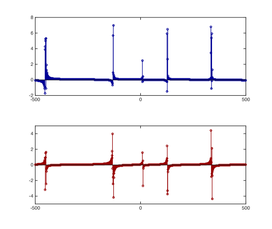
Figure 1: Real (blue) and imaginary (red) part of the FT.

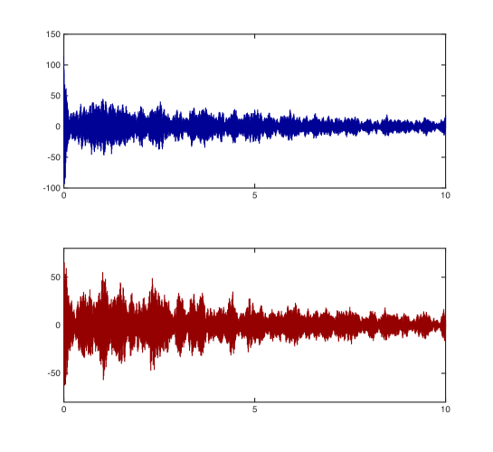
Figure 2: Real (blue) and imaginary (red) part of the signal.

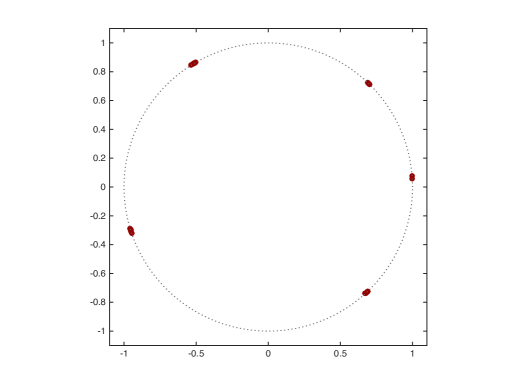
Figure 3: Generalized eigenvalues $\lambda_{i}$ for (1) with data from Table 1.

To (1) we add white Gaussian noise with SNR$=32$ dB. For comparison with our new method, we show in Figure 4 the $(\omega_{i},\beta_{i})$ results computed by means of ESPRIT using 240 samples, namely $f_{0},\ldots,f_{239}$. A signal space of dimension 20 and a noise space of dimension 40, so a total dimension $N=60$, produced a typical ESPRIT result, from a size $180\times 60$ problem. The true $(\omega_{i},\beta_{i})$ couples from Table 1 are indicated using black circles. The ESPRIT output is indicated using red bullets. So ideally every black circle should be hit by a red bullet. The ill-conditioning has clearly created a serious problem in identifying the individual input frequencies and amplitudes.

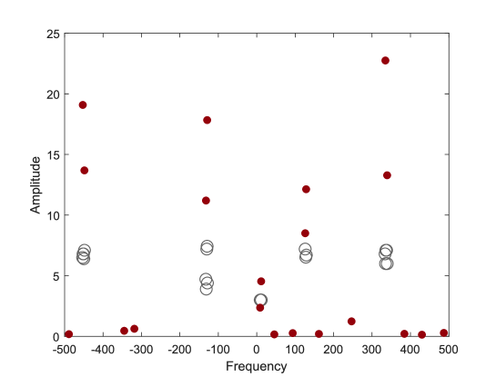
Figure 4: ESPRIT output $(\omega_{i},\beta_{i}),i=1,\ldots,20$ computed from $f_{0},\ldots,f_{239}$.

Next we choose $r=11$ and $\rho=5$. The originally clustered eigenvalues are now much better separated. To illustrate this we show in Figure 5 the noisefree generalized eigenvalues $\lambda_{i}^{r},i=1,\ldots,20$ of the $r$-fold undersampled exponential analysis problem.

With the noisy samples, we again take $N=60>n=20$ and set up a $120\times 60$ generalized eigenvalue problem (2) with the samples $f_{jr},j=0,\ldots,179$ and the $120\times 60$ Vandermonde system (9) that respectively deliver the $\lambda_{i}^{r}$ and the $\alpha_{i}$ for $i=1,\ldots,N$. With the samples $f_{jr+\rho},j=0,\ldots,59$ we set up the $60\times 60$ linear system (10) from which we compute the $\alpha_{i}\lambda_{i}^{\rho},i=1,\ldots,60$ and subsequently the $\lambda_{i}^{\rho}$. This brings our total number of samples used also to 240, comparable to the ESPRIT procedure. An advantage for ESPRIT is that the signal has less decayed in the first 240 samples, compared to the 240 samples used here. Using the Euclidean algorithm, as explicited in Lemma 2, we recover from $\lambda_{i}^{r}$ and $\lambda_{i}^{\rho}$ the true frequencies $\omega_{i}$ with $p_{1}=1,p_{2}=-2$ and $p_{1}r+p_{2}\rho=1$. With the new method we find the $(\omega_{i},\beta_{i})$ couples shown as blue dots in Figure 6. In Figure 6 the reader can even clearly count the number of frequencies retrieved in each cluster, which is the correct number when comparing to the input values in Table 1. Clearly Figure 6 is a tremendous improvement over Figure 4.

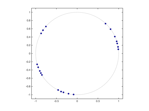
Figure 5: Generalized eigenvalues $\lambda_{i}^{r}$ for (1) with data from Table 1 and $r=11$.

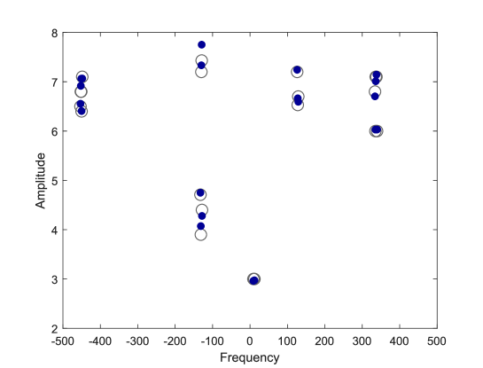
Figure 6: Output $(\omega_{i},\beta_{i}),i=1,\ldots,20$ computed from 240 samples $f_{jr+\rho},r=11,\rho=5$.

5.2 Example where collisions occur without cancellation

In Table 2 we list the $\alpha_{i}$ and $\phi_{i}$ of an exponential model, chosen in such a way that the aliasing causes terms to collide. This enables us to illustrate the workings of the technique explained in Section 4.

The bandwidth is again $\Omega=1000$ and we take $\Delta=1/\Omega$ and $r=100$. We add white Gaussian noise to the samples with SNR$=20$ dB and start our computations. When subsampling, the 6 terms collide into 3, as indicated in Figure 7 by the singular value decomposition of $H^{(0)}_{N}$ with $N=30$, which reveals its numerical rank. Actually

$$\phi(t_{rj})=(\alpha_{1}+\alpha_{2}+\alpha_{3})\exp(\phi_{1}jr\Delta)+\alpha_{4}\exp(\phi_{4}jr\Delta)+(\alpha_{5}+\alpha_{6})\exp(\phi_{5}jr\Delta).$$

We recall that $H_{N}^{(0)}$ is filled with the samples $f_{jr},j=0,\ldots,59$ and not with the samples $f_{j},j=0,\ldots,59$.

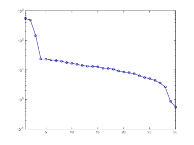
Figure 7: SVD of $H_{30}^{(0)}$ for (1) with data from Table 2 and $r=100$.

We set up the $30\times 30$ generalized eigenvalue problem (2) with the samples $f_{jr},j=0,\ldots,59$ which we solve using oeig, and the $60\times 30$ Vandermonde system (9) that respectively deliver the $\lambda_{i}^{r}$ and the $\alpha_{i}$ for $i=1,\ldots,N$. When retaining the components with largest $|\alpha_{i}|$, we find

$$\lambda_{1}^{(0)} \approx 0.36845+0.93042\mathtt{i}$$

$$\lambda_{2}^{(0)} \approx 0.36745-0.92977\mathtt{i}$$

$$\lambda_{3}^{(0)} \approx-0.72761-0.68801\mathtt{i}$$

and

$$\alpha_{1}^{(0)}=\alpha_{1}+\alpha_{2}+\alpha_{3} \approx 17.718+0.25273\mathtt{i}$$ (20)

$$\alpha_{2}^{(0)}=\alpha_{4} \approx 16.126+0.057118\mathtt{i}$$

$$\alpha_{3}^{(0)}=\alpha_{5}+\alpha_{6} \approx 4.5732-0.53331\mathtt{i}$$

At this point we have not yet been able to recover the correct $\lambda_{i}$ and $\alpha_{i}$ for the signal defined by the parameters in Table 2 (we have unearthed only 3 terms instead of 6) because of two reasons. First, the subsampling creates an aliasing effect and second the aliasing causes frequencies to collide. As explained in Section 4, we can disentangle the information in the collisions from more values $\alpha_{i}^{(1)}(k),k=1,2,\ldots$, where $\alpha_{i}^{(1)}(0)=\alpha_{i}^{(0)}$, simply because the $\alpha_{i}^{(1)}(k)$ are themselves linear combinations of exponentials. To not complicate matters too much yet, the example is cancellation free: so the correct value $n_{0}=3$ is immediately discovered from the sampling at the multiples of $r\Delta$, as we see in (20).

For the disentanglement, we choose $\rho=133$ and we set up the Vandermonde systems (17),

$$\begin{pmatrix}1&\ldots&1\\ \lambda_{1}^{(0)}&\ldots&\lambda_{3}^{(0)}\\ \vdots&&\vdots\\ (\lambda_{1}^{(0)})^{9}&\ldots&(\lambda_{3}^{(0)})^{9}\end{pmatrix}\begin{pmatrix}\alpha_{1}^{(1)}(k)\\ \alpha_{2}^{(1)}(k)\\ \alpha_{3}^{(1)}(k)\end{pmatrix}=\begin{pmatrix}f_{k\rho}\\ f_{r+k\rho}\\ \vdots\\ f_{9r+k\rho}\end{pmatrix},\qquad k=1,\ldots,11.$$

In total so far 170 samples are used. A singular value analysis of the Hankel matrices

$$\begin{pmatrix}\alpha_{i}^{(1)}(0)&\alpha_{i}^{(1)}(1)&\ldots&\alpha_{i}^{(1)}(5)\\ \alpha_{i}^{(1)}(1)&\alpha_{i}^{(1)}(2)&\ldots&\alpha_{i}^{(1)}(6)\\ \vdots&\vdots&\ddots&\vdots\\ \alpha_{i}^{(1)}(5)&\alpha_{i}^{(1)}(6)&\ldots&\alpha_{i}^{(1)}(10)\\ \end{pmatrix},\qquad i=1,2,3$$

reveals the number of components that one can distinguish in and consequently extract from the $\alpha_{i}^{(1)}(k)$. The numbers are respectively 3, 2, 1 for $i=1,2,3$ and so $h_{1}=1,h_{2}=4,h_{3}=6,h_{4}=7$. The size of these Hankel matrices filled with values $\alpha_{i}^{(1)}(k)$, is chosen somewhat larger than necessary so that the correctness of their rank is confirmed a number of times. We can also conclude that

$$n=\sum_{i=1}^{n_{0}}(h_{i+1}-h_{i})=6.$$

For $i=1,2,3$ the generalized eigenvalue problems

$$\begin{pmatrix}\alpha_{i}^{(1)}(1)&\ldots&\alpha_{i}^{(1)}(6)\\ \vdots&\ddots&\vdots\\ \alpha_{i}^{(1)}(6)&\ldots&\alpha_{i}^{(1)}(11)\\ \end{pmatrix}v_{\ell}=\lambda_{\ell}^{(1)}\begin{pmatrix}\alpha_{i}^{(1)}(0)&\ldots&\alpha_{i}^{(1)}(5)\\ \vdots&\ddots&\vdots\\ \alpha_{i}^{(1)}(5)&\ldots&\alpha_{i}^{(1)}(10)\\ \end{pmatrix}v_{\ell}$$

reveal the $\lambda_{\ell}^{(1)}=\exp(\phi_{\ell}\rho\Delta),\ell=h_{i},\ldots,h_{i+1}-1,i=1,\ldots,n_{0}$. Note that we chose a notation where the $\lambda_{\ell}^{(1)}$ are not indexed by a double index $(\ell,i),\ell=1,\ldots,h_{i+1}-h_{i},i=1,\ldots,n_{0}$ but are indexed consecutively from $\ell=h_{1}=1$ to $\ell=h_{n_{0}+1}-1=n$. This matches the indexing of the $\lambda_{\ell}^{(0)}$ of which some are coalescent, namely $\lambda_{h_{i}}^{(0)}=\cdots=\lambda_{h_{i+1}-1}^{(0)},i=1,\ldots,n_{0}$. The respective Vandermonde systems with unknowns $\alpha_{h_{i}},\ldots,\alpha_{h_{i+1}-1}$ and right hand sides $\alpha_{i}^{(1)}(0)$, $\ldots$, $\alpha_{i}^{(1)}(11)$ reveal the $\alpha_{\ell},\ell=h_{i},\ldots,h_{i+1}-1$ in (16). Again we retain only the $h_{i+1}-h_{i}$ components with largest $|\alpha_{\ell}|$. From the $\lambda_{\ell}^{(0)}=\exp(\phi_{\ell}r\Delta),\ell=h_{i},\ldots,h_{i+1}-1,i=1,\ldots,n_{0}$ and $\lambda_{\ell}^{(1)}=\exp(\phi_{\ell}\rho\Delta),\ell=1,\ldots,n$ the imaginary part of $\phi_{i}$ can be recovered as indicated in Lemma 2: with $p_{1}=4$ and $p_{2}=-3$ we have $p_{1}r+p_{2}\rho=1$ and so

$$\Im(\phi_{\ell})=4\operatorname{Arg}(\lambda_{\ell}^{(0)})\Omega-3\operatorname{Arg}(\lambda_{\ell}^{(1)})\Omega+2\pi h\Omega,\qquad 1\leq\ell\leq 6,\qquad h\in\mathbb{Z},$$

where $h$ is taken such that $0\leq\Im(\phi_{\ell})<2\pi\Omega$. Eventually we unearth the following 6 $\phi_{i}$ and $\alpha_{i}$:

$$\phi_{1} \approx-0.021600+\mathtt{i}2\pi 192.29,$$

$$\phi_{2} \approx-0.0085122+\mathtt{i}2\pi 289.87,$$

$$\phi_{3} \approx-0.025728+\mathtt{i}2\pi 386.69,$$

$$\phi_{4} \approx-0.066292+\mathtt{i}2\pi 538.18,$$

$$\phi_{5} \approx-0.043745+\mathtt{i}2\pi 858.70,$$

$$\phi_{6} \approx 0.0026126+\mathtt{i}2\pi 956.23$$

and

$$\alpha_{1} \approx 19.011+\mathtt{i}0.53818,$$

$$\alpha_{2} \approx-20.481+\mathtt{i}0.89352,$$

$$\alpha_{3} \approx 21.445-\mathtt{i}1.5790,$$

$$\alpha_{4} \approx 5.8439-\mathtt{i}0.035907,$$

$$\alpha_{5} \approx 5.0770+\mathtt{i}0.037562,$$

$$\alpha_{6} \approx 10.758-\mathtt{i}0.40878.$$

5.3 Example with cancellations in the collisions

The cancellation strategy is most clearly illustrated by means of a noisefree example, where exact cancellations are observed. The actual occurrence of this situation in case of real-life data is extremely small, but we primarily want to show that the proposed sub-Nyquist method is capable of recovering from it.

Let

$$\phi(t)=\exp(2\pi\mathtt{i}t)-\exp(2\pi\mathtt{i}21t)+\exp(2\pi\mathtt{i}41t)-\exp(2\pi\mathtt{i}61t)+\\ e^{\mathtt{i}2\pi 72/100}\exp(2\pi\mathtt{i}11t)-e^{\mathtt{i}2\pi 32/100}\exp(2\pi\mathtt{i}31t)+\exp(2\pi\mathtt{i}9t).$$ (21)

We take $\Omega=100,\Delta=0.01$ and sample $f_{j}=\phi(j\Delta)$ for particular values of $j$. With $r=5$ the first four terms cancel each other and the fifth and sixth term collide:

$$f_{5j}=0\exp(2\pi\mathtt{i}5j/100)+\left(e^{\mathtt{i}2\pi 72/100}-e^{\mathtt{i}2\pi 32/100}\right)\exp(2\pi\mathtt{i}55j/100)+\\ \exp(2\pi\mathtt{i}45j/100).$$ (22)

So from the samples $f_{0},f_{5},f_{10},\ldots$ only two terms can be retrieved:

$$\text{rank }H^{(0)}_{3}=\text{rank}\begin{pmatrix}f_{0}&f_{5}&f_{10}\\ f_{5}&f_{10}&f_{15}\\ f_{10}&f_{15}&f_{20}\end{pmatrix}=2$$

and rank $H_{N}^{(0)}=2,N\geq 2$. The 2 eigenvalues that we can already compute, are $\lambda_{5}^{(0)}=\exp(2\pi\mathtt{i}55/100)$ and $\lambda_{7}^{(0)}=\exp(2\pi\mathtt{i}45/100)$, satisfying

$$\begin{pmatrix}f_{5}&f_{10}\\ f_{10}&f_{15}\end{pmatrix}v=\lambda\begin{pmatrix}f_{0}&f_{5}\\ f_{5}&f_{10}\end{pmatrix}v.$$

From the Vandermonde system

$$\begin{pmatrix}1&1\\ \lambda_{5}^{(0)}&\lambda_{7}^{(0)}\end{pmatrix}\begin{pmatrix}\alpha_{5}^{(0)}\\ \alpha_{7}^{(0)}\end{pmatrix}=\begin{pmatrix}f_{0}\\ f_{5}\end{pmatrix}$$

we find $\alpha_{5}^{(0)}=e^{\mathtt{i}2\pi 72/100}-e^{\mathtt{i}2\pi 32/100}$ and $\alpha_{7}^{(0)}=1$. We now need to ask ourselves whether $n_{0}$ truly equals 2 or whether some cancellation of terms has happened. With $\rho=12$ we find that

$$f_{5j+12k}=\\ \left(e^{\mathtt{i}2\pi 12k/100}-e^{\mathtt{i}2\pi 52k/100}+e^{\mathtt{i}2\pi 92k/100}-e^{\i 2\pi 32k/100}\right)\exp(2\pi\mathtt{i}5j/100)+\\ \left(e^{\mathtt{i}2\pi 72/100}e^{\mathtt{i}2\pi 32k/100}-e^{\mathtt{i}2\pi 32/100}e^{\mathtt{i}2\pi 72k/100}\right)\exp(2\pi\mathtt{i}55j/100)+\\ e^{\mathtt{i}2\pi 8k/100}\exp(2\pi\mathtt{i}45j/100).$$ (23)

For $k=1$ we hit an accidental zero for the coefficient of $\exp(2\pi\mathtt{i}55j/100)$ and therefore

$$\text{rank }H^{(12)}_{3}=\text{rank}\begin{pmatrix}f_{12}&f_{17}&f_{22}\\ f_{17}&f_{22}&f_{27}\\ f_{22}&f_{27}&f_{32}\end{pmatrix}=2$$

again, with rank $H_{N}^{(12)}=2,N\geq 2$. The generalized eigenvalues satisfying

$$\begin{pmatrix}f_{17}&f_{22}\\ f_{22}&f_{27}\end{pmatrix}v=\lambda\begin{pmatrix}f_{12}&f_{17}\\ f_{17}&f_{22}\end{pmatrix}v,$$

namely $\lambda_{1}^{(0)}=\exp(2\pi\mathtt{i}5/100)$ and $\lambda_{7}^{(0)}=\exp(2\pi\mathtt{i}45/100)$, also belong to the $n_{0}$ eigenvalues that are identifiable from the evaluations at the multiples of $r\Delta$, since a shift does not change the generalized eigenvalues, only their coefficients. From the Vandermonde system

$$\begin{pmatrix}1&1\\ \lambda_{1}^{(0)}&\lambda_{7}^{(0)}\end{pmatrix}\begin{pmatrix}\alpha_{1}^{(1)}(1)\\ \alpha_{7}^{(1)}(1)\end{pmatrix}=\begin{pmatrix}f_{12}\\ f_{17}\end{pmatrix}$$

we find $\alpha_{1}^{(1)}(1)$ and $\alpha_{7}^{(1)}(1)$. Apparently $n_{0}$ equals at least 3, because in the first bunch computed from the samples $f_{5j+12k}$ with $k=0$ we find two eigenvalues and in the second bunch with $k=1$ we find one more. Bringing these results together results in the intermediate estimates

$$h_{1}=1 :\alpha_{h_{1}}^{(1)}(0)=0,\alpha_{h_{1}}^{(1)}(1)=e^{\mathtt{i}2\pi 12/100}-e^{\mathtt{i}2\pi 52/100}+e^{\mathtt{i}2\pi 92/100}-e^{\i 2\pi 32/100},$$

$$h_{2}=5 :\alpha_{h_{2}}^{(1)}(0)=e^{\mathtt{i}2\pi 72/100}-e^{\mathtt{i}2\pi 32/100},\alpha_{h_{2}}^{(1)}(1)=0,$$

$$h_{3}=7 :\alpha_{h_{3}}^{(1)}(0)=1,\alpha_{h_{3}}^{(1)}(1)=e^{\mathtt{i}2\pi 8/100},$$

where the values $h_{i}$ are merely mentioned as a guideline and are not explicitly computed. Remember that in real-life experiments the indices $h_{i}$ are not known and need not be known. They are revealed as the algorithm progresses.

Let us turn our attention to larger values of $k$ to have the current estimate $n_{0}=3$ confirmed and to extract all $n$ distinct terms. As described in Section 4 on the disentangling of collisions, we continue sampling at multiples of the shift, namely we collect the $f_{jr+k\rho}$ for $k>1$. With $k=2$ we obtain

$$f_{5j+24}=\left(e^{\mathtt{i}2\pi 24/100}-e^{\mathtt{i}2\pi 4/100}+e^{\mathtt{i}2\pi 84/100}-e^{\i 2\pi 64/100}\right)\exp(2\pi\mathtt{i}5j/100)+\\ \left(e^{\mathtt{i}2\pi 36/100}-e^{\mathtt{i}2\pi 76/100}\right)\exp(2\pi\mathtt{i}55j/100)+\\ e^{\mathtt{i}2\pi 16/100}\exp(2\pi\mathtt{i}45j/100)$$ (24)

and

$$\text{rank }H^{(24)}_{4}=\text{rank}\begin{pmatrix}f_{24}&f_{29}&f_{34}&f_{39}\\ \vdots&\mathinner{\mskip 1.0mu\raise 1.0pt\vbox{\kern 7.0pt\hbox{.}}\mskip 2.0mu\raise 4.0pt\hbox{.}\mskip 2.0mu\raise 7.0pt\hbox{.}\mskip 1.0mu}&&\vdots\\ f_{39}&\ldots&&f_{54}\end{pmatrix}=3$$

with rank $H_{N}^{(24)}=3,N\geq 4$. Merely for completeness we compute the generalized eigenvalues satisfying

$$\begin{pmatrix}f_{29}&\ldots&f_{39}\\ \vdots&\mathinner{\mskip 1.0mu\raise 1.0pt\vbox{\kern 7.0pt\hbox{.}}\mskip 2.0mu\raise 4.0pt\hbox{.}\mskip 2.0mu\raise 7.0pt\hbox{.}\mskip 1.0mu}&\vdots\\ f_{39}&\ldots&f_{49}\end{pmatrix}v=\lambda\begin{pmatrix}f_{24}&\ldots&f_{34}\\ \vdots&\mathinner{\mskip 1.0mu\raise 1.0pt\vbox{\kern 7.0pt\hbox{.}}\mskip 2.0mu\raise 4.0pt\hbox{.}\mskip 2.0mu\raise 7.0pt\hbox{.}\mskip 1.0mu}&\vdots\\ f_{34}&\ldots&f_{44}\end{pmatrix}v.$$

We find $\lambda_{1}^{(0)}=\exp(2\pi\mathtt{i}5/100),\lambda_{5}^{(0)}=\exp(2\pi\mathtt{i}55/100),\lambda_{7}^{(0)}=\exp(2\pi\mathtt{i}45/100)$, which confirms our earlier obtained combined result. Hence $n_{0}=3$. We also compute the values for $\alpha_{i}^{(1)}(2),i=1,5,7$ from the Vandermonde system

$$\begin{pmatrix}1&1&1\\ \lambda_{1}^{(0)}&\lambda_{5}^{(0)}&\lambda_{7}^{(0)}\\ (\lambda_{1}^{(0)})^{2}&(\lambda_{5}^{(0)})^{2}&(\lambda_{7}^{(0)})^{2}\end{pmatrix}\begin{pmatrix}\alpha_{1}^{(1)}(2)\\ \alpha_{5}^{(1)}(2)\\ \alpha_{7}^{(1)}(2)\end{pmatrix}=\begin{pmatrix}f_{24}\\ f_{29}\\ f_{34}\end{pmatrix}.$$

The purpose now is to find out how many terms are in the expressions $\alpha_{i}^{(1)}(k)$ for each $i$ retrieved so far. We compute $\alpha_{1}^{(1)}(k),\alpha_{5}^{(1)}(k),\alpha_{7}^{(1)}(k)$ for $k\geq 3$ from

$$\begin{pmatrix}1&1&1\\ \lambda_{1}^{(0)}&\lambda_{5}^{(0)}&\lambda_{7}^{(0)}\\ (\lambda_{1}^{(0)})^{2}&(\lambda_{5}^{(0)})^{2}&(\lambda_{7}^{(0)})^{2}\end{pmatrix}\begin{pmatrix}\alpha_{1}^{(1)}(k)\\ \alpha_{5}^{(1)}(k)\\ \alpha_{7}^{(1)}(k)\end{pmatrix}=\begin{pmatrix}f_{12k}\\ f_{5+12k}\\ f_{10+12k}\end{pmatrix},\qquad k=3,4,\ldots,$$

which reuses the $n_{0}\times n_{0}$ Vandermonde coefficient matrix from above.

Let us write $k=2\kappa-2$, so that when we increase $\kappa$ by 1 then $k$ is increased by 2. We check the rank of the $\kappa\times\kappa$ matrices

$$\begin{pmatrix}\alpha_{i}^{(1)}(0)&\ldots&\alpha_{i}^{(1)}(\kappa-1)\\ \vdots&\mathinner{\mskip 1.0mu\raise 1.0pt\vbox{\kern 7.0pt\hbox{.}}\mskip 2.0mu\raise 4.0pt\hbox{.}\mskip 2.0mu\raise 7.0pt\hbox{.}\mskip 1.0mu}&\vdots\\ \alpha_{i}^{(1)}(\kappa-1)&\ldots&\alpha_{i}^{(1)}(2\kappa-2)\end{pmatrix},\qquad i=1,5,7.$$

When pursuing the shifts up to $k=9$, meaning $\kappa=5$, we find that for $i=1$ the rank is 4, for $i=5$ the rank is 2 and for $i=7$ the rank is 1, leading to a grand total of $n=7$ distinct terms. We now separate the terms that are hiding in each of the collisions by computing the generalized eigenvalues satisfying

$$\begin{pmatrix}\alpha_{i}^{(1)}(1)&\ldots&\alpha_{i}^{(1)}(\kappa)\\ \vdots&\mathinner{\mskip 1.0mu\raise 1.0pt\vbox{\kern 7.0pt\hbox{.}}\mskip 2.0mu\raise 4.0pt\hbox{.}\mskip 2.0mu\raise 7.0pt\hbox{.}\mskip 1.0mu}&\vdots\\ \alpha_{i}^{(1)}(\kappa)&\ldots&\alpha_{i}^{(1)}(2\kappa-1)\end{pmatrix}v=\lambda\begin{pmatrix}\alpha_{i}^{(1)}(0)&\ldots&\alpha_{i}^{(1)}(\kappa-1)\\ \vdots&\mathinner{\mskip 1.0mu\raise 1.0pt\vbox{\kern 7.0pt\hbox{.}}\mskip 2.0mu\raise 4.0pt\hbox{.}\mskip 2.0mu\raise 7.0pt\hbox{.}\mskip 1.0mu}&\vdots\\ \alpha_{i}^{(1)}(\kappa-1)&\ldots&\alpha_{i}^{(1)}(2\kappa-2)\end{pmatrix}v,\\ \qquad i=1,5,7.$$ (25)

We find

$$i=1,\kappa=4: \lambda_{1}^{(1)}=\exp(2\pi\mathtt{i}12/100),\lambda_{2}^{(1)}=\exp(2\pi\mathtt{i}52/100),$$

$$\lambda_{3}^{(1)}=\exp(2\pi\mathtt{i}92/100),\lambda_{4}^{(1)}=\exp(2\pi\mathtt{i}32/100),$$

$$i=5,\kappa=2: \lambda_{5}^{(1)}=\exp(2\pi\mathtt{i}32/100),\lambda_{6}^{(1)}=\exp(2\pi\mathtt{i}72/100),$$

$$i=7,\kappa=1: \lambda_{7}^{(1)}=\exp(2\pi\mathtt{i}8/100).$$

At this stage we have all the information to reconstruct the non-aliased generalized eigenvalues:

$$\lambda_{1}^{(0)},\lambda_{1}^{(1)} \to\lambda_{1}=\exp(2\pi\mathtt{i}1/100),$$

$$\lambda_{1}^{(0)},\lambda_{2}^{(1)} \to\lambda_{2}=\exp(2\pi\mathtt{i}21/100),$$

$$\lambda_{1}^{(0)},\lambda_{3}^{(1)} \to\lambda_{3}=\exp(2\pi\mathtt{i}41/100),$$

$$\lambda_{1}^{(0)},\lambda_{4}^{(1)} \to\lambda_{4}=\exp(2\pi\mathtt{i}61/100),$$

$$\lambda_{5}^{(0)},\lambda_{5}^{(1)} \to\lambda_{5}=\exp(2\pi\mathtt{i}11/100),$$

$$\lambda_{5}^{(0)},\lambda_{6}^{(1)} \to\lambda_{6}=\exp(2\pi\mathtt{i}31/100),$$

$$\lambda_{7}^{(0)},\lambda_{7}^{(1)} \to\lambda_{7}=\exp(2\pi\mathtt{i}9/100).$$

Remains to compute the individual linear coefficients of each of the 7 terms. We compute $\alpha_{1},\alpha_{2},\alpha_{3},\alpha_{4}$ from

$$\begin{pmatrix}1&1&1&1\\ \lambda_{1}^{(1)}&\lambda_{2}^{(1)}&\lambda_{3}^{(1)}&\lambda_{4}^{(1)}\\ (\lambda_{1}^{(1)})^{2}&(\lambda_{2}^{(1)})^{2}&(\lambda_{3}^{(1)})^{2}&(\lambda_{4}^{(1)})^{2}\\ (\lambda_{1}^{(1)})^{3}&(\lambda_{2}^{(1)})^{3}&(\lambda_{3}^{(1)})^{3}&(\lambda_{4}^{(1)})^{3}\end{pmatrix}\begin{pmatrix}\alpha_{1}\\ \alpha_{2}\\ \alpha_{3}\\ \alpha_{4}\end{pmatrix}\begin{pmatrix}\alpha_{1}^{(1)}(0)\\ \alpha_{1}^{(1)}(1)\\ \alpha_{1}^{(1)}(2)\\ \alpha_{1}^{(1)}(3)\end{pmatrix},$$

the coefficients $\alpha_{5}$ and $\alpha_{6}$ from

$$\begin{pmatrix}1&1\\ \lambda_{5}^{(1)}&\lambda_{6}^{(1)}\end{pmatrix}\begin{pmatrix}\alpha_{5}\\ \alpha_{6}\end{pmatrix}\begin{pmatrix}\alpha_{5}^{(1)}(0)\\ \alpha_{5}^{(1)}(1)\end{pmatrix}.$$

The coefficient $\alpha_{7}$ is given by $\alpha_{7}=\alpha_{7}^{(0)}=\alpha_{7}^{(1)}(0)$ because there were no collisions in that term.

5.4 Full algorithm in pseudocode

An algorithm covering the eventuality of the above scenarios reads as follows. We assume that $r>1$ otherwise a classical Prony analysis applies.

So far we used the notation $n$ for the number of exponential terms in the signal, which we often don’t know up front. Moreover, the data are usually noisy, so that it is best to add another number of terms in order to model the noise. We denoted the latter in the previous sections by $N-n$ so that the total number of terms we want to identify accumulates to $N$. To this end at least $2N$ samples are required, even without breaking the Shannon-Nyquist rate. We denote the number of samples collected at the uniformly distributed points $t_{jr}$ by the number $M\geq 2N$. These allow us to build the square Hankel matrices $H^{(0)}_{N}$ and $H^{(1)}_{N}$ or somewhat larger rectangular $(M-N)\times N$ versions of these matrices. When sampling at the shifted locations $t_{jr+k\rho}$ we collect for each $k$ not $M$ but $m$ samples where $\lfloor m/2\rfloor>n$. Using the latter we can build the Hankel matrices $H^{(\rho)}_{\lfloor m/2\rfloor}$. Often the total number of samples and the amount of undersampling are dictated by the circumstances and the constraints under which the analysis is performed.

We emphasize that $n_{0}$ indicates the number of terms in the exponential sum after possible collisions, including the vanished ones due to cancellation in the coefficients. Also, the time step $\Delta\in\mathbb{R}$ satisfies $\Delta\leq 1/\Omega$. With this in mind the algorithm continues as follows.

Algorithm.

Input bounds on $n$, subsampling factor $r$ and shift term $\rho$:

• $M,N,m\in\mathbb{N}$ with $M\geq 2N,N\geq n,\lfloor m/2\rfloor>n$.

• $r\in\mathbb{N},\rho\in\mathbb{Z}$ with $r>1$ and $\gcd(r,\rho)=1$.

A0. Obtain $n_{0},\lambda_{i}^{(0)},\alpha_{i}^{(0)}$:

• Collect the samples $f_{jr}=\phi(t_{jr}),j=0,\ldots,M-1$ and estimate $n_{0}\leq n$ by the numerical rank of the matrix $H_{N}^{(0)}$.

• For one or more $1\leq k\leq 2n-1$ collect the samples $f_{jr+k\rho}=\phi(t_{jr+k\rho}),j=0,\ldots,m-1$ and compute the numerical rank $n_{k}$ of $H_{\lfloor m/2\rfloor}^{(k\rho)}$.

• From these different views on the number of collided terms in the exponential sum, we find that the correct value for $n_{0}$ is $n_{0}=\max_{k}n_{k}$.

• Compute for $i=1,\ldots,n_{0}$ the generalized eigenvalues $\lambda_{i}^{(0)}$ and the coefficients $\alpha_{i}^{(0)}$ as in Example 5.3.

• Either $N\times N$ Hankel and $2N\times N$ Vandermonde systems are used or their least squares $(M-N)\times N$ and $M\times N$ versions.

A1. Obtain $\alpha_{i}^{(1)}(k)$ and $h_{i+1}-h_{i}$ for $i=1,\ldots,n_{0}$ and $1\leq k\leq K<2n$:

Put $\alpha_{i}^{(1)}(0):=\alpha_{i}^{(0)},k=1$ and execute the for loop:

1. compute the $\alpha_{i}^{(1)}(k)$ from (17) or its $m\times n_{0}$ least squares version,

2. collect or reuse the samples $f_{jr+(k+1)\rho}=\phi(t_{jr+(k+1)\rho}),j=0,\ldots,m-1$,

3. compute the $\alpha_{i}^{(1)}(k+1)$ from (17) or its $m\times n_{0}$ least squares version,

4. compute the numerical rank $\nu_{i}(\kappa)$ of the $(\kappa+1)\times(\kappa+1)$ matrix

   $$\begin{bmatrix}\alpha_{i}^{(1)}(0)&\cdots&\alpha_{i}^{(1)}(\kappa)\\ \vdots&&\vdots\\ \alpha_{i}^{(1)}(\kappa)&\cdots&\alpha_{i}^{(1)}(k+1)\end{bmatrix},\qquad 2\kappa=k+1,$$

5. if $\nu_{i}(\kappa)=\nu_{i}(\kappa-1)$:

   • then $h_{i+1}-h_{i}=\kappa$,

   • else $k:=k+2$, collect or reuse the samples $f_{jr+k\rho},j=0,\ldots,m-1$ and goto 1.

6. compute the generalized eigenvalues $\lambda_{\ell}^{(1)},\ell=h_{i},\ldots,h_{i+1}-1$ in (18),

7. compute the $\alpha_{\ell},\ell=h_{i},\ldots,h_{i+1}-1$ from (16).

End the for loop.

Output number of terms $n$ and the parameters $\phi_{i},\alpha_{i}$:

From

• $\lambda_{\ell}^{(1)},\ell=h_{1},\ldots,h_{n_{0}+1}-1$ with $h_{1}=1,h_{n_{0}+1}-1=n$

• and $\lambda_{\ell}^{(0)}$ with $\lambda_{h_{i}}^{(0)}=\cdots=\lambda_{h_{i+1}-1}^{(0)},i=1,\ldots,n_{0}$

the $\phi_{i},i=1,\ldots,n$ can be recovered.

The $\alpha_{i},i=1,\ldots,n$ are computed from (16) as in (19).

$i$	$\alpha_{i}$	$\phi_{i}$
1	$6.5\exp(0.15\mathtt{i})$	$-0.19-\mathtt{i}2\pi 453.1$
2	$6.8$	$-0.132-\mathtt{i}2\pi 452.19$
3	$6.8\exp(0.3\mathtt{i})$	$-0.183-\mathtt{i}2\pi 451.02$
4	$6.4\exp(0.9\mathtt{i})$	$-0.11-\mathtt{i}2\pi 450.21$
5	$7.1\exp(0.7\mathtt{i})$	$-0.21-\mathtt{i}2\pi 448.39$
6	$4.71\exp(0.12\mathtt{i})$	$-0.106-\mathtt{i}2\pi 132.5$
7	$3.9\exp(0.1\mathtt{i})$	$-0.129-\mathtt{i}2\pi 131.4$
8	$7.2\exp(-0.234\mathtt{i})$	$-0.203-\mathtt{i}2\pi 130.01$
9	$7.43\exp(0.2\mathtt{i})$	$-0.16-\mathtt{i}2\pi 129.17$
10	$4.4\exp(-0.52\mathtt{i})$	$-0.19-\mathtt{i}2\pi 128.39$
11	$3\exp(0.21\mathtt{i})$	$-0.101+\mathtt{i}2\pi 9.1$
12	$3\exp(-0.8\mathtt{i})$	$-0.127+\mathtt{i}2\pi 11.81$
13	$7.2\exp(-0.106\mathtt{i})$	$-0.21+\mathtt{i}2\pi 126.01$
14	$6.53\exp(0.2\mathtt{i})$	$-0.15+\mathtt{i}2\pi 127.62$
15	$6.7\exp(-0.3\mathtt{i})$	$-0.173+\mathtt{i}2\pi 128.98$
16	$6.8\exp(-0.15\mathtt{i})$	$-0.11+\mathtt{i}2\pi 334.01$
17	$6\exp(0.26\mathtt{i})$	$-0.12+\mathtt{i}2\pi 335.18$
18	$7.1\exp(-0.2\mathtt{i})$	$-0.157+\mathtt{i}2\pi 336.01$
19	$7.1$	$-0.120+\mathtt{i}2\pi 337.91$
20	$6\exp(-0.1\mathtt{i})$	$-0.18+\mathtt{i}2\pi 339.61$

Table 1: Collision-free example.

$i$	$\alpha_{i}$	$\phi_{i}$
1	$18$	$\mathtt{i}2\pi 191.9$
2	$-20$	$\mathtt{i}2\pi 291.9$
3	$20$	$\mathtt{i}2\pi 391.9$
4	$5$	$\mathtt{i}2\pi 526.2$
5	$5$	$\mathtt{i}2\pi 858.1$
6	$11$	$\mathtt{i}2\pi 958.1$

Table 2: Example where collisions occur.

References

- [1] E. J. Candès, C. Fernandez-Granda, Towards a mathematical theory of super-resolution, Communications on Pure and Applied Mathematics 67 (6) (2014) 906–956.
- [2] A. Moitra, Super-resolution, extremal functions and the condition number of Vandermonde matrices, in: Proceedings of the Forty-seventh Annual ACM Symposium on Theory of Computing, STOC ’15, ACM, 2015, pp. 821–830.
- [3] D. W. Kammler, Approximation with sums of exponentials in , Journal of Approximation Theory 16 (4) (1976) 384–408.
- [4] J. Varah, On fitting exponentials by nonlinear least squares, SIAM Journal on Scientific and Statistical Computing 6 (1) (1985) 30–44.
- [5] B. Halder, T. Kailath, Efficient estimation of closely spaced sinusoidal frequencies using subspace-based methods, IEEE Signal Processing Letters 4 (2) (1997) 49–51.
- [6] R. Schmidt, Multiple emitter location and signal parameter estimation, IEEE Transactions on Antennas and Propagation 34 (3) (1986) 276–280.
- [7] R. Roy, T. Kailath, ESPRIT-estimation of signal parameters via rotational invariance techniques, IEEE Transactions on Acoustics, Speech, and Signal Processing 37 (7) (1989) 984–995.
- [8] Y. Hua, T. K. Sarkar, Matrix pencil method for estimating parameters of exponentially damped/undamped sinusoids in noise, IEEE Transactions on Acoustics, Speech, and Signal Processing 38 (1990) 814–824.
- [9] G. Golub, P. Milanfar, J. Varah, A stable numerical method for inverting shape from moments, SIAM Journal on Scientific Computing 21 (1999) 1222–1243.
- [10] S. Das, A. Neumaier, Solving overdetermined eigenvalue problems, SIAM Journal on Scientific Computing 35 (2) (2013) A541–A560.
- [11] G. Beylkin, L. Monzón, On approximation of functions by exponential sums, Applied and Computational Harmonic Analysis 19 (1) (2005) 17–48.
- [12] D. Potts, M. Tasche, Parameter estimation for exponential sums by approximate Prony method, Signal Processing 90 (2010) 1631–1642.
- [13] D. Potts, M. Tasche, Parameter estimation for nonincreasing exponential sums by Prony-like methods, Linear Algebra and its Applications 439 (4) (2013) 1024–1039.
- [14] H. Nyquist, Certain topics in telegraph transmission theory, Transactions of the American Institute of Electrical Engineers 47 (2) (1928) 617–644.
- [15] C. E. Shannon, Communication in the presence of noise, Proceedings of the IRE 37 (1949) 10–21.
- [16] E. J. Candès, J. Romberg, T. Tao, Robust uncertainty principles: exact signal reconstruction from highly incomplete frequency information, IEEE Transactions on Information Theory 52 (2) (2006) 489–509.
- [17] D. L. Donoho, Compressed sensing, IEEE Transactions on Information Theory 52 (4) (2006) 1289–1306.
- [18] M. Vetterli, P. Marziliano, T. Blu, Sampling signals with finite rate of innovation, IEEE Transactions on Signal Processing 50 (6) (2002) 1417–1428.
- [19] P. P. Vaidyanathan, P. Pal, Sparse sensing with co-prime samplers and arrays, IEEE Transactions on Signal Processing 59 (2) (2011) 573–586.
- [20] Z. Tan, Y. C. Eldar, A. Nehorai, Direction of arrival estimation using co-prime arrays: A super resolution viewpoint, IEEE Transactions on Signal Processing 62 (21) (2014) 5565–5576.
- [21] A. Cuyt, W.-s. Lee, Smart data sampling and data reconstruction, patent EP2745404B1.
- [22] A. Cuyt, W.-s. Lee, Smart data sampling and data reconstruction, patent US 9,690,740.
- [23] G. Plonka, M. Tasche, Prony methods for recovery of structured functions, GAMM-Mitt. 37 (2) (2014) 239–258.
- [24] P. Henrici, Applied and computational complex analysis I, John Wiley & Sons, New York, 1974.
- [25] E. Kaltofen, W.-s. Lee, Early termination in sparse interpolation algorithms, Journal of Symbolic Computation 36 (3-4) (2003) 365–400.
- [26] A. Cuyt, M. Tsai, M. Verhoye, W.-s. Lee, Faint and clustered components in exponential analysis, Applied Mathematics and Computation 327 (2018) 93–103.
- [27] B. Beckermann, G. Golub, G. Labahn, On the numerical condition of a generalized Hankel eigenvalue problem, Numerische Mathematik 106 (1) (2007) 41–68.
- [28] W. Gautschi, Norm estimates for inverses of Vandermonde matrices, Numerische Mathematik 23 (1975) 337–347.
- [29] A. Cuyt, W.-s. Lee, An analog Chinese Remainder Theorem, Tech. rep., Universiteit Antwerpen (2017).