Ferrimagnetism and compensation temperature in spin-$1/2$ Ising trilayers

Abstract

The mean-field and effective-field approximations are applied in the study of magnetic and thermodynamic properties of a spin-$1/2$ Ising system containing three layers, each of which is composed exclusively of one out of two possible types of atoms, A or B. The A-A and B-B bonds are ferromagnetic while the A-B bonds are antiferromagnetic. The occurrence of a compensation phenomenon is verified and the compensation and critical temperatures are obtained as functions of the Hamiltonian parameters. We present phase diagrams dividing the parameter space in regions where the compensation phenomenon is present or absent and a detailed discussion about the influence of each parameter on the overall behavior of the system is made.

I Introduction

The interest in studies on ferrimagnets has increased considerably in the last few decades, particularly due to a number of phenomena associated with these systems that present great potential for technological applications Connell et al. (1982); Camley and Barnaś (1989); Felser et al. (2007); Phan and Yu (2007). Since the discovery of ferrimagnetism in 1948 Cullity and Graham (2008), several theoretical models have been proposed to explain their magnetic behavior Syozi and Nakano (1955); Hattori (1966). Essentially, in these models the ferrimagnet is described as a combination of two or more magnetically coupled substructures, e. g., sublattices, layers, or subsets of atoms within the system. Each substructure may exhibit a different thermal behavior for its magnetization and the combination of these different behaviors may lead to the appearance of some interesting phenomena such as compensation points, i. e., temperatures below the critical point for which the total magnetization is zero while the individual substructures remain magnetically ordered Cullity and Graham (2008).

Mixed-spin Ising systems are often used as models to study ferrimagnetism. The occurrence of compensation in such systems has been verified in two-dimensional systems with a number of combinations of different spins (e. g. $s=1/2$, $1$, $3/2$, $2$, $5/2$) Godoy and Figueiredo (2000); Dakhama and Benayad (2000); Nakamura (2000); Abubrig et al. (2001); Boechat et al. (2000, 2002); Godoy et al. (2004); Ekiz and Erdem (2006); Ekiz (2006); Ekiz and Erdem (2006); Wang et al. (2015, 2016a, 2016b, 2017a, 2017b); Lv et al. (2017). Some single-spin systems, such as layered magnets composed of stacked non-equivalent ferromagnetic planes, have also been effectively used to model ferrimagnets. A bilayer Ising system with spin-$1/2$ and no dilution has been studied via transfer matrix (TM) Lipowski and Suzuki (1993); Lipowski (1998), renormalization group (RG) Hansen et al. (1993); Li et al. (2001); Mirza and Mardani (2003), mean-field approximation (MFA) Hansen et al. (1993), and Monte Carlo (MC) simulations Ferrenberg and Landau (1991); Hansen et al. (1993). Also the pair approximation (PA) has been applied to study similar systems such as Ising-Heisenberg bilayers Szałowski and Balcerzak (2012) and multilayers Szałowski and Balcerzak (2013) with spin-$1/2$ and no dilution. Although site dilution is a crucial ingredient for the existence of a compensation point in a single-spin system with even number of layers, even with in the diluted systems the compensation effect will be present only under very specific conditions, as has been verified through PA calculations for the Ising-Heisenberg bilayer Balcerzak and Szałowski (2014) and multilayer Szałowski and Balcerzak (2014) and through MC simulations for the Ising bilayer Diaz and Branco (2017a) and multilayer Diaz and Branco (2017b).

In contrast, for an odd number of layers, site dilution is no longer a necessary condition for the existence of compensation in a single-spin system. This was in fact confirmed in a very recent effective-field approximation (EFA) study of Ising trilayer nanostructures Santos and Barreto (2017) for a few particular cases of Hamiltonian parameter values. In order to study the conditions under which compensation effects may occur, we propose a simple model, which is treatable by theoretical approximations and may also be considerably easier to be built in experimental studies, when compared to previous ferrimagnetic models. The system we introduce in this work does not require the presence of dilution, which is time- and memory-consuming in numerical simulations and may be difficult to control in experimental set-ups. More specifically, we study a three-layer Ising model with two types of atoms (A and B, say), such that each layer is composed of only one type of atom. Only two parameters are involved, the ratios between different interactions. These parameters are changed, in order to establish the conditions for the appearance of the compensation effect. We compare two different theoretical approximations, which are easy to implement in the studied model.

The paper is organized as follows: the theoretical model for the trilayer system is presented in Sec. II, in which we present the Hamiltonian for the system in Sec. II.1, the mean-field analysis of the Hamiltonian in Sec. II.2, and the effective-field analysis in Sec. II.3. The numerical results are presented and discussed in Sec. III and our conclusion and final remarks in Sec. IV.

II Theoretical Model

II.1 Hamiltonian

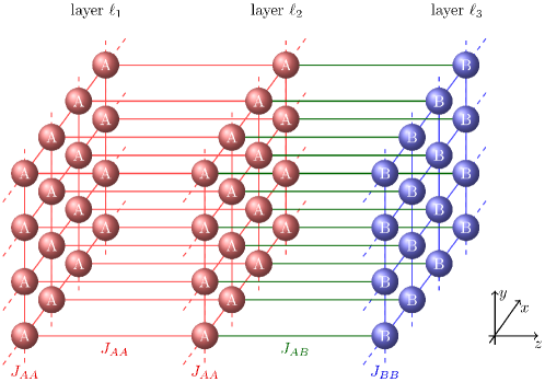
(a) AAB

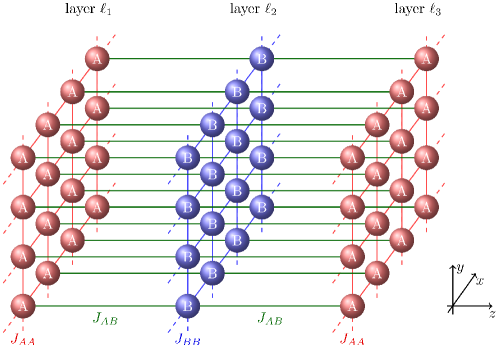
(b) ABA

Figure 1: A schematic representation of the trilayer systems. In (a), we have the AAB system, in which $J_{11}=J_{12}=J_{22}=J_{AA}>0$, $J_{23}=J_{AB}<0$, and $J_{33}=J_{BB}>0$. In (b), we have the ABA system, in which $J_{11}=J_{33}=J_{AA}>0$; $J_{12}=J_{23}=J_{AB}<0$; $J_{22}=J_{BB}>0$.

The trilayer system we study consists of three monoatomic layers, $\ell_{1}$, $\ell_{2}$, and $\ell_{3}$. Each layer is composed exclusively of either type-A or type-B atoms (see Fig. 1). The general system is described by the spin-1/2 Ising Hamiltonian

$$-\beta\mathcal{H}=\sum_{\langle i\in\ell_{1},j\in\ell_{1}\rangle}K_{11}s_{i}s_{j}+\sum_{\langle i\in\ell_{2},j\in\ell_{2}\rangle}K_{22}s_{i}s_{j}+\sum_{\langle i\in\ell_{3},j\in\ell_{3}\rangle}K_{33}s_{i}s_{j}+\sum_{\langle i\in\ell_{1},j\in\ell_{2}\rangle}K_{12}s_{i}s_{j}+\sum_{\langle i\in\ell_{2},j\in\ell_{3}\rangle}K_{23}s_{i}s_{j},$$ (1)

where the sums run over nearest neighbors, $\beta\equiv(k_{B}T)^{-1}$, $T$ is the temperature, $k_{B}$ is the Boltzmann constant, and the spin variables $s_{i}$ assume the values $\pm 1$. The couplings are $K_{\gamma\eta}\equiv\beta J_{\gamma\eta}$, where the exchange integrals $J_{\gamma\eta}$ are $J_{AA}>0$ for A-A bonds, $J_{BB}>0$ for B-B bonds, and $J_{AB}<0$ for A-B bonds.

In this work we consider the two possible configurations of the trilayer with more atoms of type-A than type-B (see Fig. 1). The AAB system is the case in which $J_{11}=J_{12}=J_{22}=J_{AA}$, $J_{23}=J_{AB}$, and $J_{33}=J_{BB}$ (Fig. 1(a)), whereas the ABA system corresponds to $J_{11}=J_{33}=J_{AA}$, $J_{12}=J_{23}=J_{AB}$, and $J_{22}=J_{BB}$ (Fig. 1(b)). In both cases we wish to calculate the magnetization in each layer, $m_{\gamma}\equiv\langle s_{i\in\ell_{\gamma}}\rangle$, $\gamma=1,2,3$, as well as the total magnetization

$$m_{\mbox{\scriptsize{tot}}}=\frac{1}{3}(m_{1}+m_{2}+m_{3}).$$ (2)

II.2 Mean-field approximation (MFA)

For our analysis of the Hamiltonian (1), we start by using the Callen identity Callen (1963) so the magnetizations can be written as

$$m_{\gamma}=\langle\tanh{(\beta E_{i\in\ell_{\gamma}})}\rangle$$ (3)

where $\langle\cdots\rangle$ denotes the canonical thermal average, and

$$\beta E_{i\in\ell_{1}} =K_{11}\sum_{\delta}s_{(i+\delta)\in\ell_{1}}+K_{12}s_{i\in\ell_{2}}$$

$$\beta E_{i\in\ell_{2}} =K_{22}\sum_{\delta}s_{(i+\delta)\in\ell_{2}}+K_{12}s_{i\in\ell_{1}}+K_{23}s_{i\in\ell_{3}}$$

$$\beta E_{i\in\ell_{3}} =K_{33}\sum_{\delta}s_{(i+\delta)\in\ell_{3}}+K_{23}s_{i\in\ell_{2}},$$ (4)

where $\gamma=1,2$ or $3$. The sums $\sum_{\delta}s_{(i+\delta)\in\ell_{\gamma}}$ are over the $z$ nearest neighbors of the $i$-th site in layer $\ell_{\gamma}$, considering only the neighbors in the same layer. For the particular case of square lattices, we have $z=4$.

In the standard mean-field approach, we have $\langle\tanh{(\beta E_{i\in\ell_{\gamma}})}\rangle=\tanh{\langle\beta E_{i\in\ell_{\gamma}}\rangle}$, such that the means in Eq. (3) become

$$m_{1} =\tanh{(zK_{11}m_{1}+K_{12}m_{2})},$$

$$m_{2} =\tanh{(zK_{22}m_{2}+K_{12}m_{1}+K_{23}m_{3})},$$

$$m_{3} =\tanh{(zK_{33}m_{3}+K_{23}m_{2})}.$$ (5)

The system (II.2) was solved numerically to determine the magnetizations $m_{1}$, $m_{2}$, $m_{3}$, and $m_{\mbox{\scriptsize{tot}}}$ as functions of the temperature for various values of the Hamiltonian parameters. The results are presented in Sec. III.

II.3 Effective-field approximation (EFA)

In order to improve the mean-field approximation results we employ the effective-field method first proposed by Honmura and Kaneyoshi Honmura and Kaneyoshi (1979). In this approach we use the differential operator $e^{\lambda D}f(x)=f(x+\lambda)$, where $D\equiv\frac{\partial}{\partial x}$, to we rewrite Eq. (3) as

$$m_{\gamma}=\langle\exp{(\beta E_{i\in\ell_{\gamma}}D)}\rangle\left.\tanh{x}\right|_{x=0},$$ (6)

where $\gamma=1,2$ or $3$, and the $\beta E_{i\in\ell_{\gamma}}$ are given by Eqs. (II.2).

Substituting (II.2) into Eq. (6), expanding the exponentials, and using the identities: $(s_{i})^{2n}=1$ and $(s_{i})^{2n+1}=s_{i}$, we obtain the following exact relations:

$$m_{1}= \langle\Pi_{\delta}\{\cosh{(K_{11}D)}+s_{(i+\delta)\in\ell_{1}}\sinh{(K_{11}D)}\}\times\{\cosh{(K_{12}D)}+s_{i\in\ell_{2}}\sinh{(K_{12}D)}\}\rangle\left.\tanh{(x)}\right|_{x=0},$$

$$m_{2}= \langle\Pi_{\delta}\{\cosh{(K_{22}D)}+s_{(i+\delta)\in\ell_{2}}\sinh{(K_{22}D)}\}\times\{\cosh{(K_{12}D)}+s_{i\in\ell_{1}}\sinh{(K_{12}D)}\}$$

$$\times\{\cosh{(K_{23}D)}+s_{i\in\ell_{3}}\sinh{(K_{23}D)}\}\rangle\left.\tanh{(x)}\right|_{x=0},$$

$$m_{3}= \langle\Pi_{\delta}\{\cosh{(K_{33}D)}+s_{(i+\delta)\in\ell_{3}}\sinh{(K_{33}D)}\}\times\{\cosh{(K_{23}D)}+s_{i\in\ell_{2}}\sinh{(K_{23}D)}\}\rangle\left.\tanh{(x)}\right|_{x=0},$$ (7)

where again the $\delta$ index indicates the products are taken over the $z$ nearest neighbors of the $i$-th site. After performing the thermal averages, neglecting multispin correlations (i. e., $\langle s_{i}s_{j}\cdots s_{k}\rangle=\langle s_{i}\rangle\langle s_{j}\rangle\cdots\langle s_{k}\rangle$), and expanding the hyperbolic sines and cosines as exponentials, it is possible to rewrite Eqs. (II.3) as:

$$m_{1}= \frac{1}{2^{z+1}}\{(1+m_{1})e^{K_{11}D}+(1-m_{1})e^{-K_{11}D}\}^{z}\times\{(1+m_{2})e^{K_{12}D}+(1-m_{2})e^{-K_{12}D}\}\left.\tanh{(x)}\right|_{x=0}$$

$$m_{2}= \frac{1}{2^{z+2}}\{(1+m_{2})e^{K_{22}D}+(1-m_{2})e^{-K_{22}D}\}^{z}$$

$$\times\{(1+m_{1})e^{K_{12}D}+(1-m_{1})e^{-K_{12}D}\}\times\{(1+m_{3})e^{K_{23}D}+(1-m_{3})e^{-K_{23}D}\}\left.\tanh{(x)}\right|_{x=0}$$

$$m_{3}= \frac{1}{2^{z+1}}\{(1+m_{3})e^{K_{33}D}+(1-m_{3})e^{-K_{33}D}\}^{z}\times\{(1+m_{2})e^{K_{23}D}+(1-m_{2})e^{-K_{23}D}\}\left.\tanh{(x)}\right|_{x=0}$$ (8)

As in Sec. II.2, the system (II.3) was solved numerically to determine the magnetizations $m_{1}$, $m_{2}$, $m_{3}$, and $m_{\mbox{\scriptsize{tot}}}$ as functions of the temperature for various values of the Hamiltonian parameters. The results are presented in Sec. III.

III Numerical Results and Discussion

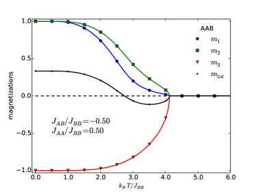
(a) With compensation (MFA).

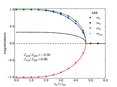
(b) Without compensation (MFA).

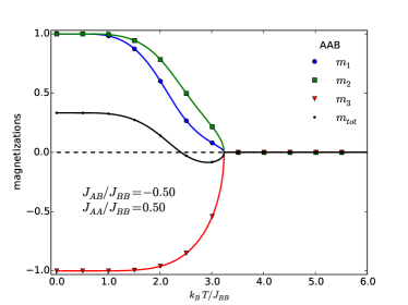
(c) With compensation (EFA).

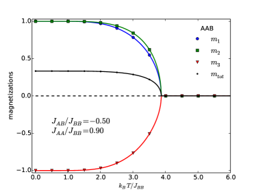
(d) Without compensation (EFA).

Figure 2: Magnetizations as functions of temperature for the AAB system with $J_{AB}/J_{BB}=-0.50$. For $J_{AA}/J_{BB}=0.50$, both mean-field (a) and effective-field (c) approximations show a compensation temperature $T_{comp}$ such that $m_{tot}=0$ and $0<T_{comp}<T_{c}$. For $J_{AA}/J_{BB}=0.90$, both mean-field (b) and effective-field (d) approximations show no compensation effect.

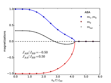
(a) With compensation (MFA).

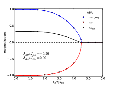
(b) Without compensation (MFA).

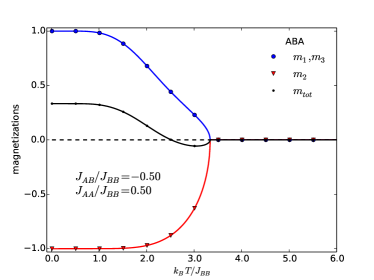
(c) With compensation (EFA).

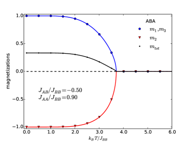
(d) Without compensation (EFA).

Figure 3: (Color online) Magnetizations as functions of temperature for the ABA system with $J_{AB}/J_{BB}=-0.50$. For $J_{AA}/J_{BB}=0.50$, both mean-field (a) and effective-field (c) approximations show a compensation temperature $T_{comp}$ such that $m_{tot}=0$ and $0<T_{comp}<T_{c}$. For $J_{AA}/J_{BB}=0.90$, both mean-field (b) and effective-field (d) approximations show no compensation effect.

We start our analysis by solving the systems in Eqs. (II.2) (MFA) and (II.3) (EFA) and looking at the temperature dependence of the magnetizations of the systems for a range of values of the Hamiltonian parameters, as shown in Figs. 2 and 3. The compensation point is determined for each set of Hamiltonian parameters as the temperature $T_{comp}$ for which $m_{\mbox{\scriptsize{tot}}}=0$, while $m_{1},m_{2},m_{3}\neq 0$. In turn, the critical point is determined as the temperature for which all magnetizations vanish simultaneously. Our goal in this work is to outline the contribution of each parameter to the presence or absence of the compensation phenomenon. To that end we map out the regions of the parameter space for which the system has a compensation point, as seen in Figs. 2(a) and 3(a) for the MFA and Figs. 2(c) and 3(c) for the EFA, and the regions for which the compensation effect does not take place, as seen in Figs. 2(b) and 3(b) for the MFA and Figs. 2(d) and 3(d) for the EFA.

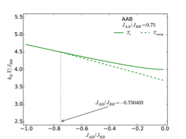
(a) MFA.

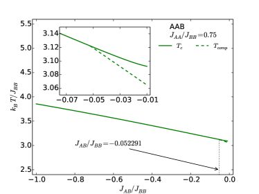
(b) EFA.

Figure 6: $T_{c}$ (full line) and $T_{comp}$ (dashed line) as functions of $J_{AB}/J_{BB}$ for the AAB system with $J_{AA}/J_{BB}=0.75$. The dotted line marks the value of $J_{AB}/J_{BB}$ for which $T_{comp}=T_{c}$ and below which there is no compensation. In (a) we present the results for the mean-field approximation, whereas in (b) the results for the effective-field approximation are depicted. The inset in (b) is a zoom in the region where the $T_{comp}$ and $T_{c}$ curves meet.

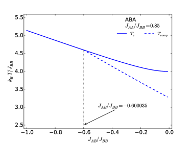
(a) MFA.

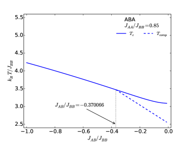
(b) EFA.

Figure 7: $T_{c}$ (full line) and $T_{comp}$ (dashed line) as functions of $J_{AB}/J_{BB}$ for the ABA system with $J_{AA}/J_{BB}=0.85$. The dotted line marks the value of $J_{AB}/J_{BB}$ for which $T_{comp}=T_{c}$ and below which there is no compensation. In (a) we present the results for the mean-field approximation, whereas in (b) the results for the effective-field approximation are depicted.

In order to analyze the influence of $J_{AA}/J_{BB}$ in the behavior of the system, we fix a value for $J_{AB}/J_{BB}$ and plot the critical temperatures and compensation temperatures as functions of $J_{AA}/J_{BB}$, as seen in Fig. 4 for the AAB system and in Fig. 5 for the ABA system, both cases for $J_{AB}/J_{BB}=-0.50$. In Figs. 4(a) and 5(a) we have the results for the mean-field approximation, whereas in Figs. 4(b) and 5(b) we have the results for the effective-field approximation. In all cases, the dotted vertical lines mark the value of $J_{AA}/J_{BB}$ at which $T_{c}=T_{comp}$ and above which there is no compensation for each system. Likewise, to understand the influence of $J_{AB}/J_{BB}$ in the behavior of the trilayers, we fix a value for $J_{AA}/J_{BB}$ and obtain $T_{c}$ and $T_{comp}$ as functions of $J_{AB}/J_{BB}$, as shown in Fig. 6 for an AAB trilayer with $J_{AB}/J_{BB}=0.75$, as well as in Fig. 7 for an ABA trilayer with $J_{AB}/J_{BB}=0.85$. In Figs. 6(a) and 7(a) we have the results for the mean-field approximation, whereas in 6(b) and 7(b) we have the results for the effective-field approximation. The dotted vertical lines mark the value of $J_{AB}/J_{BB}$ at which $T_{c}=T_{comp}$ and below which there is no compensation for each system. The inset in Fig. 7(b) is a zoom in the region where the $T_{comp}$ and $T_{c}$ curves meet.

One important aspect about the comparison between the MFA and EFA results is that the values of $T_{c}$ and $T_{comp}$ are consistently higher for the MFA than for the EFA. For instance, Figs. 2 and 3 show that for $J_{AA}/J_{BB}=0.50$ and $J_{AB}/J_{BB}=-0.50$ the MFA critical temperature is $\approx 27\%$ higher than the EFA estimate for both AAB and ABA systems. When we increase $J_{AA}/J_{BB}$ to $0.90$ while keeping $J_{AB}/J_{BB}$ constant, that percentile difference decreases to $\approx 21\%$ and $\approx 22\%$ for the AAB and ABA systems, respectively. Although the difference is slightly less pronounced, for $J_{AA}/J_{BB}=0.50$ and $J_{AB}/J_{BB}=-0.50$, the MFA compensation temperature is $\approx 14\%$ ($\approx 11\%$) higher than the EFA estimate for the AAB (ABA) trilayer. This is expected since the effective-field theory takes into account short-range correlations, which are entirely neglected by a standard mean-field approximation. Therefore, although both methods overestimate the values of critical and compensation temperatures, the values are expected to approach the true ones within the effective-field approximation framework. It is worth stressing that the same occurs when we contrast pair approximation Balcerzak and Szałowski (2014) and Monte Carlo Diaz and Branco (2017a) results for a site-diluted Ising bilayer, in which case the PA temperatures are higher than the MC ones. Although the PA takes into account longer-range correlations than both EFA and MFA, it still systematically overestimates the temperatures since it is a mean-field-like approximation. Monte Carlo simulations, on the other hand, do not neglect correlations and should therefore provide temperature estimates that are much closer to the true values than their mean-field-like counterparts.

Similarly, by analyzing Figs. 4, 5, 6, and 7, we see that the percentile difference between the MFA and EFA estimates for the critical temperatures is somewhere between $20\%$ and $35\%$, being greater for both small $J_{AA}/J_{BB}$ and small $|J_{AB}/J_{BB}|$. On the other hand, for the compensation temperatures we have percentile differences between MFA and EFA estimates ranging from $\approx 0\%$ to $30\%$, being greater for $J_{AA}/J_{BB}\rightarrow 1$ and for $|J_{AB}/J_{BB}|\rightarrow 0$. Another important difference between mean-field and effective-filed results, which also follows from Figs. 4, 5, 6, and 7, is that the area of these diagrams occupied by the ferrimagnetic phase with compensation is smaller for the EFA than it is for the MFA.

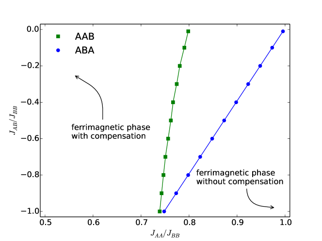
(a) MFA.

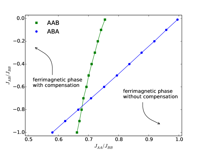
(b) EFA.

Figure 8: Phase diagrams for both AAB and ABA systems. In (a) we present the results for the mean-field approximation, whereas in (b) we present the results for the effective-field approximation.

Finally, as it follows from the analyzes presented above, it is convenient to divide the parameter space of our Hamiltonian in two distinct regions of interest. One is a ferrimagnetic phase for which there is no compensation at any temperature and the second is a ferrimagnetic phase where there is a compensation point at a certain temperature $T_{comp}$. We present the results in Fig. 8, where we plot the phase diagrams for both AAB and ABA types of trilayer and in both mean-field (Fig. 8(a)) and effective-field (Fig. 8(b)) approximations. For each type of system, the line marks the separation between a ferrimagnetic phase with compensation (to the left) and a ferrimagnetic phase without compensation (to the right). These diagrams show that the compensation phenomenon will happen for a sufficiently small $J_{AA}/J_{BB}$ irrespective of the value of $J_{AB}/J_{BB}$, although the range of values of $J_{AA}/J_{BB}$ for which the phenomenon occurs increases as the A-B interplanar coupling gets weaker. This behavior is similar to that of the diluted bilayer Balcerzak and Szałowski (2014); Diaz and Branco (2017a) and multilayer Szałowski and Balcerzak (2014); Diaz and Branco (2017b) systems for sufficiently small dilutions.

The main difference we see in Fig. 8 between systems AAB and ABA in both approximations is that the AAB trilayer is less sensitive to the value of $J_{AB}/J_{BB}$ than the ABA, as the line separating the phases is more like a straight vertical line for the former system than for the latter. This is consistent with the fact that the number of A-B bonds in the AAB trilayer is only half that of the ABA trilayer. In addition, Fig. 8 shows that the area occupied by the ferrimagnetic phase with compensation in the $J_{AB}\times J_{AA}$ diagram is smaller for the EFA than it is for the MFA for both types of trilayer, confirming the trend seen in Figs. 4, 5, 6, and 7. We see the same behavior when we compare the PA Balcerzak and Szałowski (2014) and MC Diaz and Branco (2017a) results for the Ising bilayer, in which case the smaller area is obtained through Monte Carlo simulations, i. e., the area seems to decrease as we use more accurate approximations. Thus, we expect that in future theoretical works on the trilayer systems, the area of the phase with compensation will be smaller in the PA and even smaller in MC simulations than what we obtained in this work for both EFA and MFA.

IV Conclusion

We studied the thermodynamic and magnetic properties of an Ising trilayer model. The system is composed of three planes, each of which can only have atoms of one out of two types (A or B). The interactions between pairs of atoms of the same type (A-A or B-B bonds) are ferromagnetic while the interactions between pairs of atoms of different types (A-B bonds) are antiferromagnetic. The study is carried out through both a mean-field and an effective-field approaches. The magnetic behavior of the system as a function of the temperature is obtained numerically. We verified the occurrence of a compensation phenomenon and determined the compensation temperatures, as well as the critical temperatures of the model for a range of values of the Hamiltonian parameters.

We present phase diagrams and a detailed discussion about the conditions for the occurrence of the compensation phenomenon. For instance, we see that the phenomenon is only possible if the $J_{AA}<J_{BB}$ and that the range of values of $J_{AA}/J_{BB}$ for which there is compensation increases as $|J_{AB}/J_{BB}|$ gets smaller, as it is also the case for similar systems containing a mixture of ferromagnetic and antiferromagnetic bonds Balcerzak and Szałowski (2014); Szałowski and Balcerzak (2014); Diaz and Branco (2017a). The summary of the results is presented in a convenient way on $J_{AB}\times J_{AA}$ diagrams for both types of trilayer and for both mean-field and effective-field approximations. These diagrams separate the Hamiltonian parameter-space in two distinct regions: one corresponding to a ferrimagnetic phase where the system has a compensation point and the other is a ferrimagnetic phase without compensation.

It is clear from these diagrams that the area of the parameter space occupied by the ferrimagnetic phase with compensation is smaller in the EFA than it is in the MFA for both types of trilayer. Thus, in a more sophisticated approach, this area could be even smaller. However, we believe the compensation effect obtained here is robust and cannot be just an artifact of the mean-field-like methods used in this work. The fact that there are more atoms of type A than B in the system, coupled with the fact that the antiferromagnetic interaction between atoms of different types favors the antiparallel alignment of the spins of atoms A and B, causes the system to exhibit a remanent magnetization for $T\rightarrow 0$. Since the three layers are coupled with non-null exchange integrals, all three magnetizations will go to zero at the same critical temperature; therefore it is expected that a careful choice of the Hamiltonian parameters may lead to situations where the individual magnetizations cancel each other out below the critical point. Nevertheless, a confirmation of the occurrence of the phenomenon by more sophisticated theoretical methods, such as pair approximation or Monte Carlo simulations, as well as the experimental realization of a trilayer system with characteristics similar to the model presented in this work would be of great value.

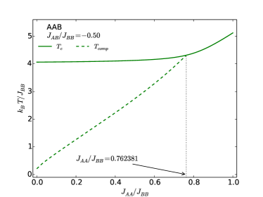
(a) MFA.

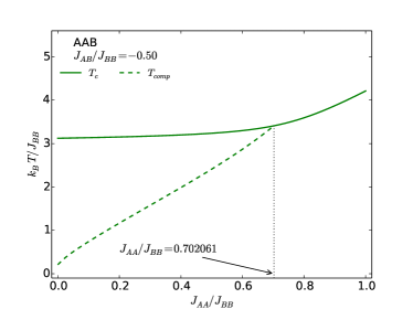
(b) EFA.

Figure 4: $T_{c}$ (full line) and $T_{comp}$ (dashed line) as functions of $J_{AA}/J_{BB}$ for the AAB system with $J_{AB}/J_{BB}=-0.50$. The dotted line marks the value of $J_{AA}/J_{BB}$ for which $T_{comp}=T_{c}$ and above which there is no compensation. In (a) we present the results for the mean-field approximation, whereas in (b) the results for the effective-field approximation are depicted.

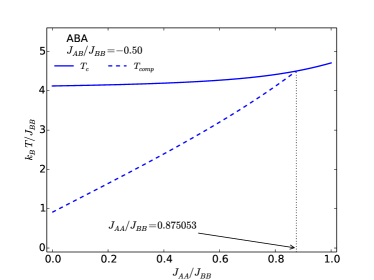
(a) MFA.

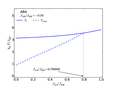
(b) EFA.

Figure 5: $T_{c}$ (full line) and $T_{comp}$ (dashed line) as functions of $J_{AA}/J_{BB}$ for the ABA system with $J_{AB}/J_{BB}=-0.50$. The dotted line marks the value of $J_{AA}/J_{BB}$ for which $T_{comp}=T_{c}$ and above which there is no compensation. In (a) we present the results for the mean-field approximation, whereas in (b) the results for the effective-field approximation are depicted.