Approximate homogenization of convex nonlinear elliptic PDEs

Abstract.

We approximate the homogenization of fully nonlinear, convex, uniformly elliptic Partial Differential Equations in the periodic setting, using a variational formula for the optimal invariant measure, which may be derived via Legendre-Fenchel duality. The variational formula expresses $\overline{H}(Q)$ as an average of the operator against the optimal invariant measure, generalizing the linear case. Several nontrivial analytic formulas for $\overline{H}(Q)$ are obtained. These formulas are compared to numerical simulations, using both PDE and variational methods. We also perform a numerical study of convergence rates for homogenization in the periodic and random setting and compare these to theoretical results.

1. Introduction

We consider homogenization of the periodic, convex, uniformly elliptic Hamilton-Jacobi-Bellman operator

(1) $$H(Q,y)=\sup_{\alpha\in{\mathcal{A}}}L_{\alpha}(Q,y)=\sup_{\alpha\in{\mathcal{A}}}\left\{-A(y,\alpha):Q+h(y,\alpha)\right\}.$$

Note that $H(Q,y)$ is convex in $Q$. Let ${\mathcal{A}}$ be a convex compact control set, and let $A:{\mathbb{T}^{d}}\times{\mathcal{A}}\to{\mathcal{S}^{d}}$ and $h:{\mathbb{T}^{d}}\times{\mathcal{A}}\to\mathbb{R}$ be continuous, where ${\mathcal{S}^{d}}$ is the space of $d\times d$ symmetric matrices, and ${\mathbb{T}^{d}}$ is the $d$-dimensional torus. We assume that $A$ is uniformly elliptic, with $0\ll\lambda I\ll A\ll\Lambda I$.

We will make use of the following result, which follows from Theorem 1.3 below. Consider an admissible control $\alpha(y)$. Let $L_{\alpha}$ be the corresponding linear operator, and let $\overline{L_{\alpha}}(Q)$ the homogenized linear operator. Then

(2) $$\overline{L_{\alpha}}(Q)\leq\overline{H}(Q)$$

with equality when $\alpha(y)$ is optimal, or, equivalently, when the control corresponds to the linearization about the corresponding solution of the cell problem, $Q+D^{2}u^{Q}(y)$.

In Section 2 we consider three example problems. One example is the maximum of two linear operators. In this case, we obtain a formula for $\overline{H}(Q)$, which is new (as far as we know). The second example is one dimensional, but with a quadratic nonlinearity. In this case, by considering constant controls, we find a lower bound for $\overline{H}(Q)$ which is numerically verified to be sharp.

Finally, we consider a two dimensional Pucci operator on stripes. In [FO] we homogenized Pucci operators, mainly with checkerboard coefficients. There we did not require convexity of the operator. We obtained accurate results for values of $Q$ away from the singularities of the operators by simply linearizing the operator about $Q$. However, for stripes coefficients, the linearization about $Q$ is not accurate. Here, we linearize about a control, and find the optimal constant control which corresponds to a control direction which depends on both the eigenvectors of $Q$ and the orientation of the stripes. When compared numerically to $\overline{H}(Q)$, this control gives very accurate results, away from the singularities. Near the singularities, there is still a small nonzero error. In [FO] we also established upper bounds for the linear homogenization error. These estimates included a term which decreased with the distance to the singular set of the operators. Similar results apply here as well.

We compared our estimates for $\overline{H}(Q)$ to numerical results. We computed $\overline{H}(Q)$ numerically using two methods: by solving the PDE for the cell problem, and by using linear programming to solve for the invariant measure. We also considered the case of random coefficients, and we found that very similar formulas for $\overline{L_{\alpha}}(Q)$ hold in the random setting.

We also computed rates of convergence for $\overline{H}(Q)$. In the periodic case, we obtained second order convergence rates, $\mathcal{O}(\varepsilon^{2})$, in one dimension. In the random setting we obtained a convergence rate of $\mathcal{O}(\varepsilon^{1/2})$, again in one dimension. These are consistent with the theoretical results we mention below.

1.1. Related work

We know of few analytical solutions $\overline{H}(Q)$, other than the formula for a separable Hamiltonian in one dimension which can be found in the early paper [LPV87]. In [FO] we obtained a formula for a separable second order operator in one dimension

$$\overline{a(y)F_{0}(Q)}=\operatorname{HM}(a)F_{0}(Q),\qquad y\in\mathbb{R}^{1}$$

where $\operatorname{HM}(a)$ is the harmonic mean of the coefficient $a(y)$. In general, the harmonic mean formula on the right hand side is a lower bound. However, in [FO] we found examples of Pucci type operators where the numerically compute value of $\overline{H}(Q)$ is very close to the right hand side, for values of $Q$ away from the corners of the operator.

For a general reference on theoretical and numerical homogenization in this context, we refer to the review paper [ES08].

A numerical method which uses the $\inf\sup$ formula for the first order case was developed in [GO04]. In [OTV09] we studied homogenization of convex (first order) Hamilton-Jacobi equations; some exact formulas in the periodic setting can be found there. Recently [CC16] studied numerical homogenization of mainly first order equations, along with one dimensional second order equations. In [CG08] the problem of homogenization of a Pucci type equation with checkerboard coefficients was studied. In that case, our results are close to, but different from theirs, see [FO].

In the random setting, the first qualitative homogenization results for fully nonlinear uniformly elliptic operators were obtained in [CSW05], followed by [CS10] which established a logarithmic estimate for convergence rates in strongly mixing environments. Algebraic convergence estimates were established in [AS14], where it was shown that in a uniformly mixing environment,

$$\mathbb{P}\left[\|u^{\varepsilon}-\bar{u}\|_{\infty}\geq C\varepsilon^{\beta}\right]\leq C\varepsilon^{\beta},$$

where $C$ and $\beta$ are constants that do not depend on $\varepsilon$. In the periodic case [CM09], proved that the order of convergence for the cell problem is $\mathcal{O}(\varepsilon^{2})$, when the HJB operator does not depend on first order terms or the macroscopic scale.

1.2. Background Theory

In the periodic uniformly convex setting, the homogenized operator can be obtained by solving the cell problem.

Definition 1.1 (Cell problem).

Given $H$ as in (1), for each $Q\in{\mathcal{S}^{d}}$, there is a unique value $\overline{H}(Q)$ and a periodic function $u^{Q}(y)$ which is a viscosity solution of the cell problem

(3) $$H(Q+D^{2}u^{Q}(y),y)=\overline{H}(Q).$$

Because the operator $H$ is uniformly elliptic, one can show that both the value $\overline{H}(Q)$ and the solution $u^{Q}$ exist and are unique, and that $u^{Q}\in C^{2}({\mathbb{T}^{d}})$ [Eva89].

In the linear case, we may use the Fredholm Alternative to find the invariant measure, and the homogenized operator is then obtained by averaging against the invariant measure, see for example [BLP11] and [FO09]. That is, under an integral compatibility condition, there is a unique invariant probability measure, $\rho$, which solves $D^{2}:(A(y)\rho)=0$, and the homogenized PDE operator is $\bar{L}(Q)=\bar{A}:Q+\bar{h}$ where $\bar{A}=\int_{\mathbb{T}^{d}}A\,\mathrm{d}\rho$ and $\bar{h}=\int_{\mathbb{T}^{d}}h\,\mathrm{d}\rho$.

In the nonlinear case, the homogenized operator may still be found by averaging against the optimal invariant measure [Gom05], or [IMT16].

Definition 1.2 (Optimal invariant measure).

Let $\Pr({\mathbb{T}^{d}}\times{\mathcal{A}})$ denote the space of Borel probability measures on ${\mathbb{T}^{d}}\times{\mathcal{A}}$. For $\rho\in\Pr({\mathbb{T}^{d}}\times{\mathcal{A}})$, we say $\rho$ is an invariant measure if $L_{0}^{*}\rho(y,\alpha)=0$ hold in the weak sense, by which we mean

(4) $$\int_{{\mathcal{A}}\times{\mathbb{T}^{d}}}A(y,\alpha(y)):D^{2}\varphi(y)\,\mathrm{d}\rho(y,\alpha)=0,\quad\forall\varphi\in C^{2}({\mathbb{T}^{d}}).$$

Define

(5) $$\bar{H}_{LP}(Q)=\sup_{\rho\in\Pr({\mathbb{T}^{d}}\times{\mathcal{A}})}\left\{\int L_{\alpha}(Q,y)\,\mathrm{d}\rho(y,\alpha)~{}\Big{|}~{}L_{0}^{*}\rho=0\right\},$$

The result follows from duality and convex analysis, in particular the theorem of Fenchel-Rockafeller. The fact that (5) and (3) give the same value is established in Theorem 1.3.

Theorem 1.3.

Let $\overline{H}(Q)$ be defined by (3) and $H_{LP}(Q)$ be defined by (5). Then

$$\overline{H}(Q)=\bar{H}_{LP}(Q).$$

Remark 1.4.

The formula above expresses an optimal invariant measure as a maximizer of the functional in (5), and the homogenized operator as the average of $L_{\alpha}(Q,y)$ against an optimal invariant measure.

Note that while the optimal invariant measure depends on $Q$, the set of invariant measures does not. This allows us to sometimes find $\bar{H}(Q)$ for all $Q$ once the invariant measures are determined. While $\bar{H}(Q)$ does not depend on how we represent $H(Q,y)$ in (1), the set of invariant measure does. So a more concise representation of the operator can lead to a smaller set of invariant measures.

2. Estimates from Linearization

In this section we apply (2), by considering specific operators where we can obtain analytical values for the homogenized linear operator $\overline{L_{\alpha}}(Q)$.

2.1. Pucci type operators on stripes

Consider the following Pucci type operator.

Definition 2.1.

Let $y\in{\mathbb{T}}^{2}$ and $Q\in\mathcal{S}^{2}$. Write $\lambda_{\text{max}}(Q),\lambda_{\text{min}}(Q)$ for the maximum and minimum eigenvalues of $Q$, respectively. Given $A(y)\geq a(y)>0$, define the convex Pucci type operator

(6) $$F^{A,a}(Q,y)=a(y)\operatorname{Tr}Q+b(y)\lambda_{\text{max}}^{+}(Q)$$

where $b(y)=A(y)-a(y)$ and $t^{+}:=\max\left\{t,0\right\}$

Remark 2.2.

The operator (6) can be rewritten

(7) $$F^{A,a}(Q,y)=a(y)\operatorname{Tr}Q+b(y)\sup_{\left|\mathbf{v}\right|=1,\mathbf{v}=0}\left\{\mathbf{v}^{\intercal}Q\mathbf{v}\right\}$$

When $Q$ is negative definite, the operator is linear, and we obtain the harmonic mean. The level sets of this operator have corners on the negative axes and on the positive diagonal in the $\lambda_{1}-\lambda_{2}$ plane. Elsewhere, the operator is linear in $\lambda_{1}$ and $\lambda_{2}$.

For the rest of the discussion we restrict to $Q$ with at least one positive eigenvalue.

Homogenization Formula 1 (Pucci with stripes).

Consider $F^{A,a}(Q,y)$ given by (6) in dimension $d=2$. Consider piecewise constant stripes, with

(8) $$a(y_{1})=1,\qquad b(y_{1})=\begin{cases}0,\quad 0\leq y_{1}\leq\frac{1}{2}\\ b_{0},\quad\frac{1}{2}\leq y_{1}\leq 1\end{cases}$$

For $Q\not\preceq 0$ and for $t\in[0,1]$ define

$$\overline{L_{t}}(Q)=\operatorname{Tr}Q+\frac{b_{0}}{2+b_{0}t}\left(q_{22}+t(q_{11}-q_{22})+2q_{12}\sqrt{t-t^{2}}\right),$$

Then

(9) $$\overline{F^{A,a}}(Q)\geq\sup_{t\in[0,1]}\overline{L_{t}}(Q),\quad Q\not\preceq 0$$

and

$$\operatorname{HM}(a)\operatorname{Tr}Q,\quad Q\preceq 0.$$

Remark 2.3.

This formula is obtained by considering constant controls in the direction of a given unit vector. We homogenize the linearization about this control, and then optimize over the choice of unit vector. In two dimensions, these unit vectors are determined by a single parameter.

The term in (9) can be simplified further analytically, but the formula becomes complicated. It is more convenient to solve it numerically using one variable equation solvers.

Proof.

We need only consider the case $Q\not\preceq 0$ since the operator is linear otherwise.

1. Since we are on stripes, we restrict to invariant measures which depend only on $y_{1}$. Given any choice of control $\alpha(y_{1})$, the equation for the invariant measure is

$$\partial_{11}\left(c(y_{1})p_{\alpha(y_{1})}(y_{1})\right)=0,\quad c(y_{1})=a(y_{1})+b(y_{1})\alpha(y_{1}).$$

and the corresponding invariant measure is $p_{\alpha(\cdot)}(y_{1})=\frac{\operatorname{HM}(c(y_{1}))}{c(y_{1})}.$

2. Next with coefficients given by (8), restrict to $\alpha(y_{1})$ constant on $b(y_{1})=b_{0}$.

3. In two dimensions, parameterize the unit vectors $(\cos\theta,\sin\theta)$ by $\mathbf{v}_{\alpha}=(\sqrt{\alpha},\sqrt{1-\alpha})$, for $\alpha=\cos^{2}\theta$, and write

(10) $$B_{\alpha}=\mathbf{v}_{\alpha}\mathbf{v}_{\alpha}^{\intercal}=\left[\begin{matrix}\alpha&\sqrt{\alpha(1-\alpha)}\\ \sqrt{\alpha(1-\alpha)}&1-\alpha\end{matrix}\right]$$

so that (7) becomes

$$F^{A,a}(Q,y)=\operatorname{Tr}Q+b(y)\sup_{\alpha\in[0,1]}\operatorname{Tr}B_{\alpha}Q$$

For these measures, the homogenized linear operator becomes

(11) $$\operatorname{HM}(a)\operatorname{Tr}Q+\int_{{\mathbb{T}}^{1}}b(y_{1})\operatorname{Tr}\left(B_{\alpha}Q\right)p_{\alpha}(y)dy$$

after integrating out the invariant measure from the Laplacian term.

Use the representation $B_{\alpha}$ given by (10) to simplify (11) to obtain the expression which is maximized in (9). ∎

2.2. Maximum of two linear operators

Definition 2.4.

Given a (constant) symmetric positive definite matrix, $A$, positive functions $a_{0}(y),a_{1}(y)>0$, and the constant $h$. Define

(12) $$H(Q,y)=\max\{a_{0}(y),a_{0}(y)+a_{1}(y)\}A:Q+h$$

Homogenization Formula 2 (Maximum of two linear operators).

Let $H(Q,y)$ be given by (12). Then

(13) $$\bar{H}(Q)=\max\{-\operatorname{HM}(a_{0})A:Q,-\operatorname{HM}(a_{0}+a_{1})A:Q\}+h$$

Proof.

Write

$$H(Q,y)=\max_{\alpha\in[0,1]}L_{\alpha}(Q,y),\quad L_{\alpha}(Q,y)\equiv-(a_{0}(y)+\alpha a_{1}(y))A:Q+h$$

1. For any choice $\alpha(y)$, the corresponding invariant measure defined by $L_{\alpha(y)}(Q,y)$, is given by

$$p_{\alpha}(y)=\frac{\operatorname{HM}(b(y,\alpha(y))}{b(y,\alpha(y))},\quad b(y,\alpha(y))=a_{0}(y)+\alpha(y)a_{1}(y).$$

and

$$\overline{L_{\alpha(y)}}(Q)=\int_{\mathbb{T}^{d}}L_{\alpha(y)}(Q,y)\,\mathrm{d}p_{\alpha}(y)=\operatorname{HM}(b(y,\alpha(y)))A:Q+h$$

So from (2), we have

$$\overline{H}(Q)=\sup_{\alpha(\cdot)}\overline{L_{\alpha(y)}}(Q)$$

Notice that $b=(a_{0}(y)+\alpha a_{1}(y))$ is increasing in $\alpha$ for each $y$. Moreover, it is easy to verify that the Harmonic Mean is an increasing function of $b$. Thus, depending on the sign of $A:Q$, the optimal value is achieved by either $\alpha(y)\equiv 0$ or $\alpha(y)\equiv 1$, accordingly. This gives (13). ∎

2.3. A one dimensional quadratic operator

Definition 2.5.

Consider for constants, $c$, $a>0$ and for the function $b(y)\geq 0$,

$$H(Q,y)=aQ+b(y)(Q^{+})^{2}-c.$$

It easy to verify that

$$H(Q,y)=\max_{\alpha\in[0,Q]}L_{\alpha}(Q,y),\quad L_{\alpha}(Q,y)=\big{(}a+2b(y)\alpha\big{)}Q-\big{(}b(y)\alpha^{2}+c\big{)}.$$

Homogenization Formula 3.

Let $H(Q,y)$ be given as in Definition 2.5. Consider the one dimensional case, $d=1$, and suppose $b$ is piecewise constant,

(14) $$b(y)=\begin{cases}0,\quad 0\leq y\leq\frac{1}{2}\\ b_{0},\quad\frac{1}{2}\leq y\leq 1\end{cases}$$

Then

(15) $$\overline{H}(Q)\geq a(Q+Q^{+})-c+\frac{a^{2}}{b_{0}}-\frac{1}{b_{0}}\sqrt{a^{3}(a+2b_{0}Q^{+})}.$$

Proof.

Consider constant controls $\alpha(y)\equiv\alpha$. In this case the invariant measure $p_{\alpha}(y)$ is given by

(16) $$p_{\alpha}(y)=\begin{dcases}\frac{a+2b_{0}\alpha}{a+b_{0}\alpha},\quad 0\leq y\leq\frac{1}{2}\\ \frac{a}{a+b_{0}\alpha},\quad\frac{1}{2}\leq y\leq 1.\end{dcases}$$

and

(17) $$\bar{L}_{\alpha}(Q) =\langle L_{\alpha},p_{\alpha}\rangle$$

(18) $$=\frac{a\left(a+2b_{0}\alpha\right)}{a+b_{0}\alpha}\left[Q-\frac{1}{2}\left(\frac{c}{a}+\frac{b_{0}\alpha^{2}+c}{a+2b_{0}\alpha}\right)\right].$$

By (2),

$$\overline{H}(Q)\geq\max_{\alpha\in[0,Q]}\overline{L_{\alpha}}(Q)$$

Next, maximize over $\alpha$. This is accomplished by solving for the roots of the derivative of this expression with respect to $\alpha$. We obtain

(19) $$\alpha^{*}(Q)=\frac{1}{b_{0}}\left(-a+\sqrt{a(a+2b_{0}Q^{+})}\right).$$

Thus the estimate is givenby (18) with $\alpha$ given by (19). Upon simplification, we obtain (15). ∎

3. Numerical results

Here we compare the results of Section 2 with the numerical homogenization of the operators.

Remark 3.1 (Numerical methods).

$\overline{H}(Q)$ was computed with two methods. In the first, the equation (1) was discretized with finite differences. A steady state solution was computed iteratively by Euler step to the parabolic equation $u_{t}+H(Q+D^{2}u,y)$. We used a filtered scheme [FO13] to choose between a monotone finite difference scheme and standard accurate finite differences. However the standard finite difference scheme was always chosen by the filtered scheme, likely because solutions are $C^{2}$ and periodic.

We also computed $\bar{H}_{LP}(Q)$ by discretizing the control space ${\mathcal{A}}$ and formulating the problem (5) as a discrete linear programming problem. Derivatives were discretized via standard second order finite differences. We then solved this LP using the package CVX [GB14, GB08] with the SeDuMi solver [Stu99].

Throughout we set $h(y,\alpha)=c=1$, and subtracted this constant from $\overline{H}(Q)$, so as to avoid trivial solutions.

3.1. Pucci type operator on stripes

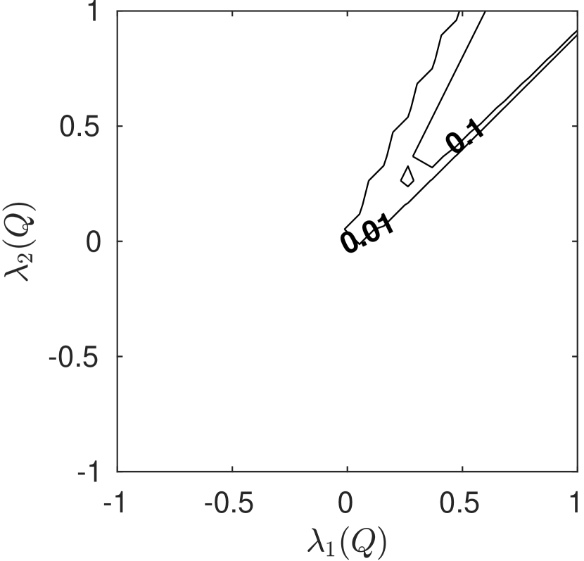
(a) Optimal Linearization error

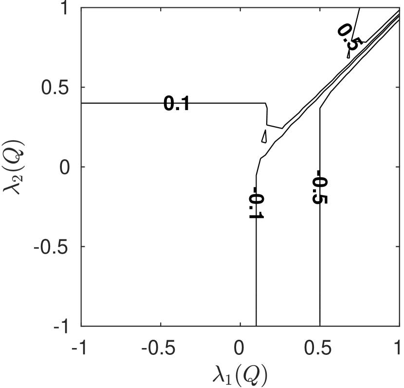
(b) Linearization error

Figure 1. Comparison between homogenization error using an invariant measure, and by homogenizing the linearized operator. In this example the operator is given by (8), with $b_{0}=2$. Here $Q=\text{diag}(\lambda_{1},\lambda_{2})$. In the third quadrant, the operator is linear, and the error was zero up to machine precision. Figure 1(a): error of Formula 1, the error is $110-8$ is most of the domain, with the $110-2$ level set shown. Figure 1(b): error of homogenizing the linearized operator. There the error is order one, outside the third quadrant.

We compared the analytical formula, Homogenization Formula 1, with numerically homogenized values. This required solving a one-variable optimization problem. We used piecewise constant coefficients, where the operator was either $\operatorname{Tr}Q$, or $F^{3,1}(Q)=1\operatorname{Tr}Q+2\lambda_{\text{max}}^{+}(Q)$. The error profile of the analytic lower bound against the numerical homogenization is plotted in Figure 1(a), for a set of diagonal $Q$. In the vicinity of the line $\lambda_{1}(Q)=\lambda_{2}(Q)$ the error is on the order of $110-1$; elsewhere the error is less than $110-2$.

We contrast this homogenization approach with the method of homogenizing the linearized operator [FO]. The homogenizing error by first linearizing the operator is much greater than the error given by Formula 1, as can be seen by comparing Figures 1(a) and 1(b).

There is a symmetry in $\bar{H}(Q)$. We represent

$$Q=R_{\phi}^{T}\text{diag}(\lambda_{1},\lambda_{2})R_{\phi}$$

where $R_{\phi}$ is a rotation matrix. When $\phi=\pi/4$, the orientation of the stripes is at an equal angle to the eigenvectors of $Q$, then $\bar{H}(Q)$ is symmetric about $\lambda_{1}=\lambda_{2}$. More generally $\bar{H}(Q)$ is symmetric under reflections in the angle about the same line of symmetry:

$$\bar{H}(Q|_{\phi=\pi/4-\gamma})=\bar{H}(Q|_{\pi/4+\gamma}),\qquad\text{for $|\gamma|\leq\pi/4$.}$$

3.2. Maximum of two linear operators, in one and two dimensions

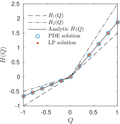
Figure 2. Validation of Formula 2, homogenization of the maximum of two linear operators, (12). Lines represent $\bar{H}(Q)$ and each of the operators $H_{i}(Q)$.

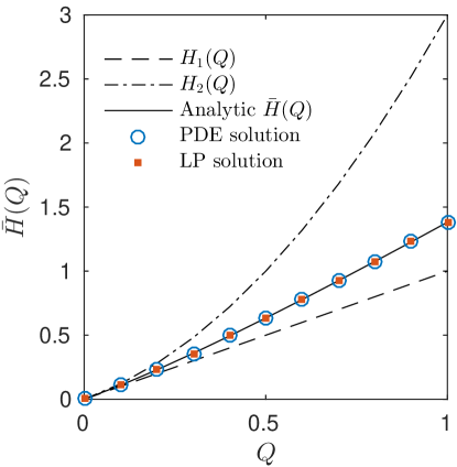
Figure 3. Validation of Formula 3. Value of $H_{1}(Q),H_{2}(Q)$, the numerically homogenized operators, and the analytic homogenized operator.

We numerically validated Homogenization Formula 2, for the maximum of two linear operators. We considered the case when the dimension is one, and we took $A=1$. The interval $[0,1]$ was discretized into $20$ equal sized pieces. The coefficients $a_{0}(y)$ and $a_{1}(y)$ were piecewise constant on these equal-sized pieces. We took $h(y)$ to be constant. In Figure 2 we let $a_{0}$ alternate between $1$ and $\frac{1}{2}$, and let $a_{1}$ alternate between $\frac{3}{2}$ and $\frac{5}{2}$. The values of the analytically homogenized operator are indistinguishable from the numerically computed values, for discrete values of $Q$, using both the direct method and the dual method. Even at the discontinuity $Q=0$, the formula agrees with the numerical homogenization up to machine precision. For reference, we also plotted $H_{1}(Q)=\min_{y}H(Q,y)$ and $H_{2}(Q)=\max_{y}H(Q,y)$. We computed many different examples and obtained similar results. (Note in this example, the invariant measure is piecewise quadratic, so the numerical method is very accurate.) We also visualized the numerical invariant measure, and found that it agreed with our formula.

We also numerically validated Formula 2 in two dimensions, and obtained similar results: in this case the analytic formula and the numerical simulations agree up to $110-12$.

3.3. The quadratic operator

Next we considered the example from §2.3, Homogenization Formula 3, for the operator

$$H(Q,y)=aQ+b(y)(Q^{+})^{2}-c.$$

Here $c$ is a constant. We numerically homogenized this operator on the periodic domain $[0,1]$, divided into 20 pieces. The coefficients are piecewise constant on equal intervals. As illustrated in Figure 3 the analytic homogenization and the numerically homogenized operator are indistinguishable. As in the previous operator (maximum of two linear operators), even at $Q=0$ the formula agrees with the numerical homogenization up to machine precision. Again, we also plot $H_{1}(Q)=\min_{y}H(Q,y)=aQ$ and $H_{2}(Q)=\max_{y}H(Q,y)=aQ+b_{0}(Q^{+})^{2}$.

4. Numerical rates of convergence in the periodic and random case

Using the exact analytical formulas of Section 2 (Formula 2 and Formula 3), we investigate empirical rates of convergence of the small-scale solutions $u^{\varepsilon}$ to the solution $\bar{u}$ of the homogenized operator. Although our theoretical results were for the periodic case, we found that the same formulas applied in the random case. This allows us to study empirical convergence rates in the random case as well.

We solved the Dirichlet problem with zero boundary conditions on the interval $[0,1]$ for the two different operators, in both the random and periodic case. The operators were the maximum of two linear operators, Formula 2; and the quadratic operator, Formula 3. These are both one dimensional examples.

We used a sequence of decreasing cell sizes, of width $\varepsilon$. We used 1 grid point per cell.

We also solved the same problem with the homogenized operator. Numerically we obtained two solutions, $u^{\varepsilon}$, and $\bar{u}$ corresponding to

(20) $$\begin{dcases}H^{\varepsilon}(D^{2}u^{\varepsilon}(x),x)=1\\ u^{\varepsilon}(x)=0,\quad x\in\partial[0,1]\end{dcases}\qquad\text{ and }\quad\begin{dcases}\bar{H}(D^{2}\bar{u}(x),x)=1\\ \bar{u}(x)=0,\quad x\in\partial[0,1].\end{dcases}$$

We chose coefficients which were piecewise constant. Let $H^{\varepsilon}(Q,x)$ be the operator parameterized by checkerboard square width $\varepsilon$. We checked convergence for both the periodic case, and the random case. In the periodic case, the unhomogenized operator alternates between two constituent operators $H_{1}$ and $H_{2}$ between the checkerboard cells. In the random case, in each checkerboard square we randomly sample from the two constituent operators with probability $\frac{1}{2}$.

In the random case, we observed convergence rates consistent with $\mathcal{O}(\varepsilon^{\frac{1}{2}})$ in the sup-norm for both operators. In the periodic case, we observed convergence rates consistent with $\mathcal{O}(\varepsilon^{2})$.

Figure 4 presents the observed rates of convergence as $u^{\varepsilon}\to\bar{u}$ in the sup-norm. In the periodic setting, the order is nearly $\mathcal{O}(\varepsilon^{2})$: we estimate that the order of convergence is $\mathcal{O}(\varepsilon^{1.95})$. In the random setting, we solved each problem 20 times, drawing the random checkerboard anew at each iteration. We then used least squares to estimate the order of convergence. We summarize these convergence estimates in Table 1. It appears that convergence in the sup-norm is roughly $\mathcal{O}(\varepsilon^{\frac{1}{2}})$ on the random checkerboard. We also measured the errors in the $\ell^{2}$ and $\ell^{1}$ norms.

Operator	Periodic, $\|\cdot\|_{\infty}$	Random, $\|\cdot\|_{\infty}$	Random, $\|\cdot\|_{2}$	Random, $\|\cdot\|_{1}$
Max of two in 1D	1.95	0.51	0.49	0.50
Quadratic in 1D	1.95	0.48	0.42	0.41

Table 1. Empirical rates of convergence for the two operators.

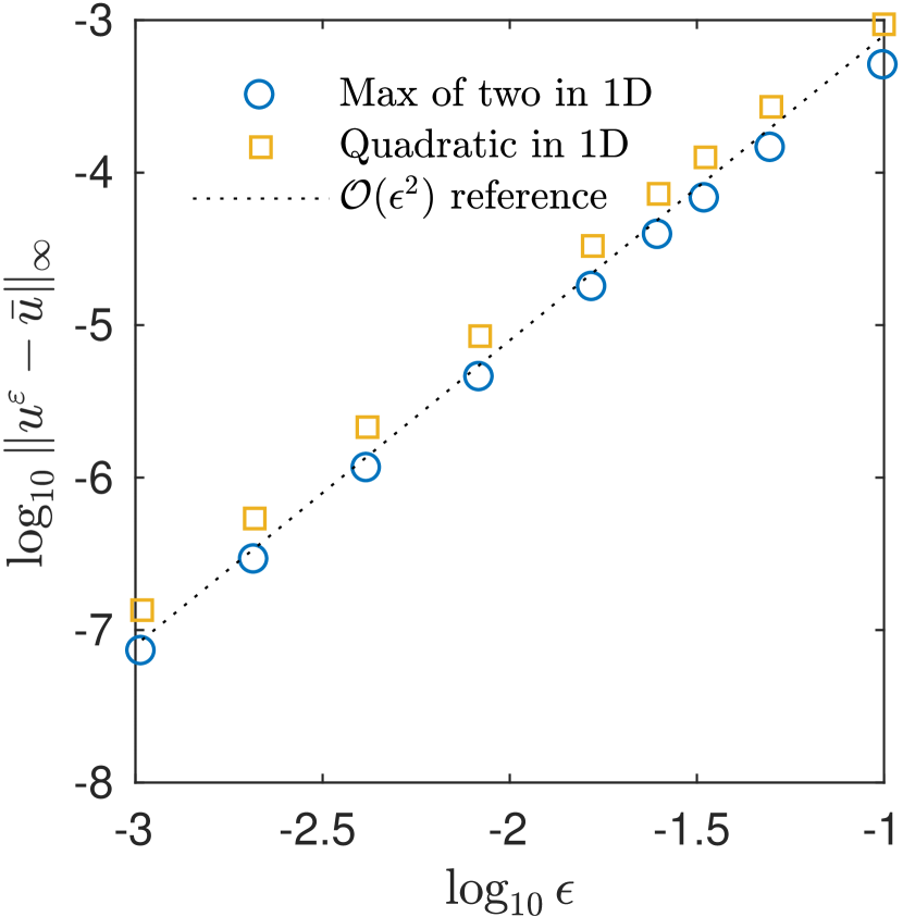
(a) Periodic convergence

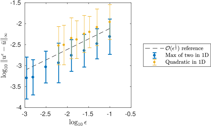
(b) Random convergence

Figure 4. Figure 4: Periodic coefficients: rate of convergence $u^{\varepsilon}\to\bar{u}$. Figure 4(b): Random coefficients: rate of convergence. We plot 90% confidence intervals for a normal distribution.

5. Conclusions

In this article we investigated the accuracy of approximating nonlinear homogenization by the homogenization of a linearization of the operator. In previous work [FO], we simply linearized about a constant. There, we obtained very accurate for checkerboard type coefficients, but significant errors in the case of stripes. In this article, we restricted to convex operators. This allowed us to write operators as the supremum of linear operators. For any linearization over a choice of control $\alpha(y)$

$$\overline{L_{\alpha}}(Q)\leq\overline{H}(Q)$$

with equality when $\alpha(y)$ is optimal.

We applied this formula to three examples. For the example of a maximum of two linear operators, we obtained an exact result, given by the maximum of two harmonic means (see (13)). For a quadratically nonlinear one dimensional operator, we restricted to piecewise constant controls and optimized over the value of the control. This results in a lower bound which was verified by numerical simulations to be exact.

Finally, we consider the Pucci-type operator with stripe coefficients. In this case, the controls depended on a choice of direction vector, which in two dimensions resulted in a one parameter optimization problem for $\overline{L_{\alpha}}(Q)$. The solution of this problem was verified by numerical simulations to be nearly exact over parameter values away from the singularities of the operator. For other values of $Q$ it achieved a small (a few percentages) relative error.

We also consider the numerical convergence rates of the homogenization problem in the scale parameter, obtaining results consistent with recent analytical results, in both the periodic and random case.

References

- [AS14] Scott N. Armstrong and Charles K. Smart. Quantitative Stochastic Homogenization of Elliptic Equations in Nondivergence Form. Archive for Rational Mechanics and Analysis, 214(3):867–911, December 2014.
- [BLP11] Alain Bensoussan, Jacques-Louis Lions, and George Papanicolaou. Asymptotic analysis for periodic structures, volume 374. American Mathematical Soc., 2011.
- [CC16] Simone Cacace and Fabio Camilli. Ergodic problems for Hamilton-Jacobi equations: yet another but efficient numerical method. arXiv preprint arXiv:1601.07107, 2016.
- [CG08] LA Caffarelli and Roland Glowinski. Numerical solution of the dirichlet problem for a pucci equation in dimension two. application to homogenization. Journal of Numerical Mathematics, 16(3):185–216, 2008.
- [CM09] Fabio Camilli and Claudio Marchi. Rates of convergence in periodic homogenization of fully nonlinear uniformly elliptic PDEs. Nonlinearity, 22(6):1481, 2009.
- [CS10] Luis A Caffarelli and Panagiotis E Souganidis. Rates of convergence for the homogenization of fully nonlinear uniformly elliptic pde in random media. Inventiones mathematicae, 180(2):301–360, 2010.
- [CSW05] Luis A Caffarelli, Panagiotis E Souganidis, and Lihe Wang. Homogenization of fully nonlinear, uniformly elliptic and parabolic partial differential equations in stationary ergodic media. Communications on pure and applied mathematics, 58(3):319–361, 2005.
- [ES08] Björn Engquist and Panagiotis E Souganidis. Asymptotic and numerical homogenization. Acta Numerica, 17:147–190, 2008.
- [Eva89] Lawrence C Evans. The perturbed test function method for viscosity solutions of nonlinear PDE. Proceedings of the Royal Society of Edinburgh: Section A Mathematics, 111(3-4):359–375, 1989.
- [FO09] Brittany D. Froese and Adam M. Oberman. Numerical averaging of non-divergence structure elliptic operators. Communications in Mathematical Sciences, 7(4):785–804, 2009.
- [FO13] Brittany D. Froese and Adam M. Oberman. Convergent filtered schemes for the Monge-Ampère partial differential equation. SIAM J. Numer. Anal., 51(1):423–444, 2013.
- [FO] Chris Finlay and Adam M Oberman. Approximate homogenization of fully nonlinear elliptic PDEs: estimates and numerical results for Pucci type equations.
- [GB08] Michael Grant and Stephen Boyd. Graph implementations for nonsmooth convex programs. In V. Blondel, S. Boyd, and H. Kimura, editors, Recent Advances in Learning and Control, Lecture Notes in Control and Information Sciences, pages 95–110. Springer-Verlag Limited, 2008. http://stanford.edu/~boyd/graph_dcp.html.
- [GB14] Michael Grant and Stephen Boyd. CVX: Matlab software for disciplined convex programming, version 2.1. http://cvxr.com/cvx, March 2014.
- [GO04] Diogo A Gomes and Adam M Oberman. Computing the effective Hamiltonian using a variational approach. SIAM journal on control and optimization, 43(3):792–812, 2004.
- [Gom05] Diogo Aguiar Gomes. Trends in Partial Differential Equations of Mathematical Physics, chapter Duality Principles for Fully Nonlinear Elliptic Equations, pages 125–136. Birkhäuser Basel, Basel, 2005.
- [IMT16] Hitoshi Ishii, Hiroyoshi Mitake, and Hung V. Tran. The vanishing discount problem and viscosity mather measures. part 1: The problem on a torus. Journal de Mathématiques Pures et Appliquées, 2016.
- [LPV87] Pierre-Louis Lions, George Papanicolaou, and Srinivasa RS Varadhan. Homogenization of Hamilton-Jacobi equations. 1987.
- [OTV09] Adam M Oberman, Ryo Takei, and Alexander Vladimirsky. Homogenization of metric Hamilton-Jacobi equations. Multiscale Modeling & Simulation, 8(1):269–295, 2009.
- [Stu99] Jos F Sturm. Using SeDuMi 1.02, a MATLAB toolbox for optimization over symmetric cones. Optimization methods and software, 11(1-4):625–653, 1999.