Automatic estimation of attractor invariants

Abstract

The invariants of an attractor have been the most used resource to characterize a nonlinear dynamics. Their estimation is a challenging endeavor in short-time series and/or in presence of noise. In this article, we present two new coarse-grained estimators for the correlation dimension and for the correlation entropy. They can be easily estimated from the calculation of two U-correlation integrals. We have also developed an algorithm that is able to automatically obtain these invariants and the noise level in order to process large data sets. This method has been statistically tested through simulations in low-dimensional systems. The results show that it is robust in presence of noise and short data lengths. In comparison with similar approaches, our algorithm outperforms the estimation of the correlation entropy.

1 Introduction

Correlation dimension (${D}$) and correlation entropy (${K_{2}}$) are quantities that characterize the natural measure of an attractor. The first one can be interpreted as the dimension of the attractor. It is a rough measure of the effective number of degrees of freedom (number of variables) involved in the dynamical process. The correlation entropy is a measure of the rate at which pairs of nearby orbits diverge. In other words, it gives us an estimate of the unpredictability of the system [6].

The correlation dimension and entropy allow us to measure the complexity of a dynamical system. Typically, more complex systems have higher dimensions and larger values of entropy. More important, these quantities help us to identify changes in the system’s complexity. For this reason, they have become very popular and widely used in the biomedical field [27], not only to characterize the dynamics of physiological systems, but also to detect different types of pathologies. For example, Choi et al. used the correlation dimension calculated from voice signal to characterize the dynamics of the phonatory system in normal and pathological conditions. They reported a mean value of $D=1.57$ for normal voices and an increased dimension value for pathological ones [3]. In Hosseinifard et al. [15] used ${D}$, among other nonlinear measures, extracted from electroencephalographic signals to classify between depressed and normal patients. Combining these features with machine learning techniques, they achieved a $90\%$ classification accuracy. On the other hand, in [9, 8] the authors illustrated how ${K_{2}}$ and other related entropy measures have been used to characterize different biological phenomena.

Since the natural measure of an attractor is invariant under the dynamical evolution, both ${D}$ and ${K_{2}}$ can be easily estimated from indirect time measurements of one of the system variables [19]. For an observed stationary time series of length $N$, $\left\{x_{n}\right\}_{n=1}^{N}$, the reconstructed $m$-dimensional delay vectors $\bm{x_{i}}=\E{x_{i},x_{i+\tau}\dots,{x_{i-\E{m-1}\tau}}}$, $i=1,2,\dots,L=N-\E{m-1}\tau$, must be formed. Here $m$ is the embedding dimension and $\tau$ is the embedding lag. As a collection, these delay vectors constitute the reconstructed attractor of the system in $\mathbb{R}^{m}$. From another point of view, this collection can be thought as samples drawn from the natural measure of the system. These samples can be used to estimate the invariants ${D}$ and ${K_{2}}$ using the correlation integral $G_{m}\E{h}$. This last quantity is defined as the probability that the distance $\tilde{z}=\norm{\bm{x_{i}}-\bm{x_{j}}}$ between two randomly selected $m$-dimensional delay vectors $\bm{x_{i}}$ and $\bm{x_{j}}$ is smaller than a value $h$ [6]:

$$G_{m}\E{h}=\int{g\E{h,\tilde{z}}f_{{\Z}}^{m}\!\E{\tilde{z}}\,\text{d}\tilde{z}},$$ (1)

where $g$ is a kernel function and $f_{{\Z}}^{m}\!\E{\tilde{z}}$ is the probability density function (pdf) of the distance between pairs of delay vectors. In this article, the Euclidean distance is used, but others measures of distance can be employed. The Grassberger and Procaccia correlation integral ${{C}_{m}\left(h\right)}$ uses as kernel function $g\E{h,\tilde{z}}=H\E{1-\tilde{z}/h}$, where $H\E{\cdot}$ is the Heaviside step function [11]. On the other hand, the Gaussian kernel correlation integral (GCI) ${{T}_{m}\left(h\right)}$ proposed by Diks et al. [5] adopts $g\E{h,\tilde{z}}=\exp\E{-\tilde{z}^{2}/4h^{2}}$. For deterministic time series and in absence of noise, both correlation integrals scale as:

$$C_{m}\E{h}=T_{m}\E{h} \sim h^{D}e^{{{-m\Delta t\tau K_{2}}\mathord{\vphantom{-m\Delta t\tau K_{2}}\kern-1.2pt}}}.$$

$$\text{for}\quad m\to\infty\,\,\,\text{and}\,\,\,h\to 0,$$

where $\Delta t=1/f_{s}$, being $f_{s}$ the sampling frequency of the time series. This behavior is due to that, in the attractor of a chaotic dynamical system, the expected density of points within a ball of small radius $h$, scales as $h^{D}$. Thus, the greater the correlation dimension, the more complex the attractor, and the longer it takes to revisit the same region in it [2]. On the other hand, the $e^{{{-m\Delta t\tau K_{2}}\mathord{\vphantom{-m\Delta t\tau K_{2}}\kern-1.2pt}}}$ factor is related to the exponential divergence of nearby trajectories. The higher the entropy values, the faster those trajectories diverge [7, 12].

The main advantage of the GCI over the Grassberger and Procaccia correlation integral is that the former allows us to model the influence of additive noise on the scaling law. For a time series with added white Gaussian noise of variance $\sigma^{2}$, the scaling rule is [5, 28, 22]:

$${T_{m}\E{h}}\sim \,\,{h^{m}}\E{h^{2}+\sigma^{2}}^{\frac{D-m}{2}}e^{{{-m\Delta t\tau K_{2}}\mathord{\vphantom{-m\Delta t\tau K_{2}}\kern-1.2pt}}}$$

$$\text{for}\quad m\to\infty\,\,\,\text{and}\,\,\sqrt{h^{2}+\sigma^{2}}\to 0.$$ (2)

In presence of noise, it is very important to be able to quantify its level ${\sigma}$ in order to correct the estimation of ${D}$ and ${K_{2}}$. Moreover, an imprecise estimate of these invariants can lead to mistaken conclusions about the studied phenomena. In this sense, an estimate of the noise level must be reported allowing other researchers to be aware of the limitations of the data.

The main problem of the GCI is that it requires high values of $m$ to obtain a convergent estimate of ${K_{2}}$ [22, 25]. This is a major drawback, since high values of $m$ imply much longer time series in order to achieve good estimations.

The cause of this problem is related with the kernel function of the GCI. It can be seen in Eq. (1) that the pdf of the interpoint distance depends on the embedding dimension. However, the Gaussian kernel function does not change with $m$, and, for this reason, the convergence of the GCI to the ${K_{2}}$ is slowed down [24].

As a solution we have recently proposed the U-correlation integral (UCI) [24]:

$$U_{m}^{\beta}\E{h}=\int{\frac{\Igf{\beta/2}{z/h^{2}}}{\Gf{\beta/2}}\hat{f}_{m}\E{\sigma;z}\,\text{d}z},$$ (3)

where $\Igf{a}{t}$ is the upper incomplete Gamma function, $\Gf{a}$ is the Gamma function and $\hat{f}_{m}\E{\sigma;z}$ is the pdf of the squared interpoint distance. There are two important issues about this correlation integral that deserve further analysis. First, note that the UCI’s kernel function, given by:

$$g\E{h,\beta,z}=\frac{\Igf{\beta/2}{z/h^{2}}}{\Gf{\beta/2}}$$

has a parameter $\beta$ that is used to incorporate information about the embedding dimension. In other words, this kernel function is able to change according to $m$. Second, we are now working with the square of the interpoint distance, i.e., $z=\tilde{z}^{2}$, to reduce the computational cost.

In order to find the scaling behavior of the UCI, we need an expression for the pdf of the squared distances between pairs of noisy delay vectors $\hat{f}_{m}\E{\sigma;z}$ [23, see Eq. (18)]:

$$\hat{f}_{m}\E{\sigma;z}= \frac{z^{m/2-1}}{2\E{2\sigma}^{m\!-\!D}}\frac{\Gf{D/2}}{\Gf{m/2}}$$

$$\times\Hf{\frac{m\!-\!D}{2}}{\frac{m}{2}}{-\frac{z}{4\sigma^{2}}},$$ (4)

where $\Hf{a}{b}{t}$ is the Kummer’s confluent hypergeometric function. This distribution arises under the assumption that, in absence of noise, the pdf of the pairwise distances between $m$-dimensional delay vectors (points in the reconstructed attractor) behaves as $h^{D-1}$ for a certain range of $h$ values [23]. If each of the coordinates of these vectors is perturbed with white Gaussian noise of variance $\sigma^{2}$, then the pdf of the perturbed distances will follow Eq. (4).

The scaling law for the UCI can be obtained by substituting Eq. (4) in Eq. (3) and integrating over $z$ [24]:

$$\UCi{m}{\beta}\E{h}= \frac{\widehat{\phi}}{2}\E{2\sigma}^{D}\frac{\Gf{D/2}\Gf{\E{\beta\!+\!m}/{2}}}{\Gf{\beta/2}\Gf{m/2\!+\!1}}e^{{{-m\Delta t\tau K_{2}}\mathord{\vphantom{-m\Delta t\tau K_{2}}\kern-1.2pt}}}$$

$$\!\!\times\!\!\E{\frac{h^{2}}{4\sigma^{2}}}^{m/2}\!\!\!\HF{\frac{\beta\!+\!m}{2}}{\frac{m\!-\!D}{2}}{\frac{m\!+\!2}{2}}{-\frac{h^{2}}{4\sigma^{2}}},$$ (5)

where $\hat{\phi}$ is a normalization constant and $\HF{a}{b}{c}{t}$ is the Gauss hypergeometric function.

In practical applications, once the scaling law has been selected and the correlation integral has been calculated, there are two main options to estimate ${D}$, ${K_{2}}$ and ${\sigma}$. The first one is to estimate these invariants through a nonlinear fitting of the scaling rule [5, 28]. This method is highly dependent on the range of scale selected to fit the model, and there is not a consensus about the correct way to choose it [19]. The second option is to use coarse-grained estimators. These are explicit expressions for $D$, $K_{2}$, and $\sigma$ as functions of $m$ and $h$ [6]. For example, in [22] Nolte et al. have proposed a set of coarse-grained functions based on the GCI. The most important aspect of their approach is that the calculation of these functions only depends on the estimation of ${{T}_{m}\left(h\right)}$ for two consecutive values of the embedding dimension $m$. Nevertheless, given that these estimators are based on the GCI, the convergence to ${K_{2}}$ needs high values of $m$ and, therefore, large amounts of data.

In [24] we have proposed a set of coarse-grained estimators for ${D}$, ${K_{2}}$ and ${\sigma}$ based on the UCI. However, these estimators are highly dependent on a precise estimation of ${\sigma}$.

In this article we present a new set of coarse-grained estimators for ${D}$ and ${K_{2}}$, based on the UCI, that only needs the calculation of two U-correlation integrals i. e. they do not require the a priori estimation of any quantity. Moreover, we propose a methodology to automatically estimate these invariants and the noise level of the time series.

In Section 2 we derive the here proposed coarse-grained estimators. Section 3 is devoted to describe the algorithm to automatically estimate the invariants. In Section 4 we discuss these results and give some suggestions for the practical of the algorithm. Finally, the conclusions are presented in Section 5.

2 Theory

Following a similar approach to one given by Nolte et al. [22], the here proposed coarse-grained estimators are based on a noise level functional. This quantity, closely related to the noise level of the time series, can be estimated using two U-correlation integrals. In this work, the noise level functional will be employed to correct the deviation of the coarse-grained estimators from the scaling law in presence of noise.

2.1 Noise level functional

The noise level functional based on the UCI can be defined as [24]:

$$\Delta_{m}^{\scriptscriptstyle{U}}\E{h} =\frac{1}{2}\E{\dot{D}^{\beta=m}_{m+2}\E{h}-\dot{D}_{m}^{\beta=m}\E{h}}$$

$$\approx\frac{4\sigma^{2}}{h^{2}+4\sigma^{2}}\qquad\text{for}\,\,m\gg D,$$ (6)

where

$$\dot{D}^{\beta}_{m}\E{h}={\frac{\text{d}\,{\ln\UCi{m}{\beta}\E{h}}}{\text{d}\,{\ln h}}}.$$

As it can be observed from Eq. (6), $\Delta_{m}^{\scriptscriptstyle{U}}\E{h}$ is a function that decreases monotonically from $1$ to $0$ on a scale that is proportional to the value of ${\sigma}$. This functional depends on the logarithmic derivative of two U-correlation integrals: $\UCi{m\phantom{+1}}{\beta=m}\E{h}$ and $\UCi{m+2}{\beta=m}\E{h}$. Note that the parameter $\beta$ is set equal to $m$ in both correlation integrals.

In order illustrate the behavior of this noise level functional, we will use the Henon map:

$$\begin{cases}x_{n+1}=1-ax_{n}^{2}+y_{n}&\\ y_{n+1}=bx_{n}&\end{cases},$$

where $a=1.4$ and $b=0.3$. This map has been widely used in the literature to numerically characterize different methods devoted to estimate attractor’s invariants [26, 23, 20, 6, 28, 22, 19, 25, 16, 4]. For this map, and the given parameters values, the correlation dimension and correlation entropy are ${D}$ $=1.22$ and ${K_{2}}$ $=0.3$, respectively [28].

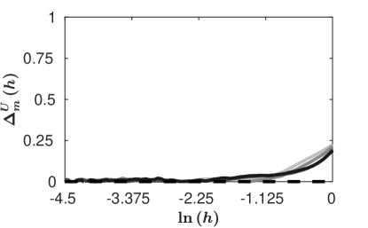
(a)

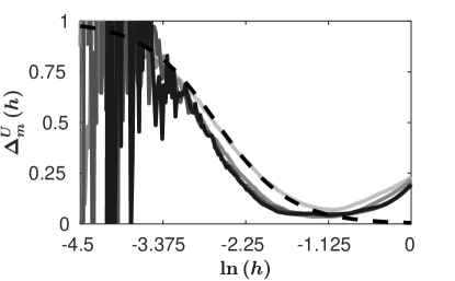
(b)

Figure 1: Henon map: Noise level functional for ${m=\left\{2,4,6,8\right\}}$, the curves for different $m$ values are color-coded in grayscale where the lightest gray corresponds to $m=2$. (a) Noiseless. (b) $\sigma=0.05$. The theoretical curve (right-hand side of Eq. (6)) is shown in dashed black line.

The noise level functionals for both a clean and a noisy ($\sigma=0.05$) realizations of the Henon map of length $N=10000$ are shown in Fig. 1. Note that in absence of noise (Fig. 1a), this functional is close to zero for a wide range of $h$ values regardless the value of $m$. On the other hand, in Fig. 1b it can be observed that $\Delta_{m}^{\scriptscriptstyle{U}}\E{h}$ falls of from $1$ to $0$ and the curves for different $m$ values are very close to the theoretical curve for $\sigma=0.05$. We must point out that the closest curve of this functional to the theoretical value is the one corresponding to $m=2$. For larger values of $m$, $\Delta_{m}^{\scriptscriptstyle{U}}\E{h}$ slightly deviates from this behavior.

2.2 Noise level coarse-grained estimator

Starting from Eq. (6), we have derived the coarse-grained noise level estimator [24]:

$$\CSu\E{h}=\frac{h}{2}\sqrt{\frac{\Delta_{m}^{\scriptscriptstyle{U}}\E{h}}{1-\Delta_{m}^{\scriptscriptstyle{U}}\E{h}}}.$$ (7)

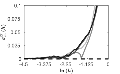
(a)

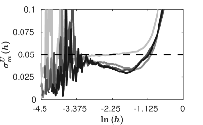
(b)

Figure 2: Henon map: Noise level coarse-grained estimator for $m=\left\{2,4,6,8\right\}$, the curves for different $m$ values are color-coded in grayscale where the lightest gray corresponds to $m=2$. (a) Noiseless. (b) $\sigma=0.05$. The true value of the noise level is shown in dashed black line.

We must point out that all time series used in this work were rescaled to have unitary standard deviation. In consequence, $\sigma$ is the noise level after rescaling, i.e.,

$$\sigma=\frac{\sigma_{n}}{\sqrt{\sigma_{c}^{2}+\sigma_{n}^{2}}},$$

where $\sigma_{n}^{2}$ is the noise variance and $\sigma_{c}^{2}$ is the variance of the clean time series. In this sense $\sigma\to 0$ corresponds to clean time series and $\sigma\to 1$ implies only noise. The signal to noise ratio (SNR) can be calculated as:

$$\text{SNR}=10\log_{10}\E{\frac{1-\sigma^{2}}{\sigma^{2}}}\,\text{dB}.$$

In Fig. 2, it is shown the coarse-grained estimator for noise level as a function of $h$ for $m=\left\{2,4,6,8,10\right\}$ for both a clean and a noisy ($\sigma=0.05$) realization of the Henon map with length $N=10000$. It can be observed in Fig. 2a that, for the noiseless case, $\CSu\E{h}$ approaches to zero as $h\to 0$. On the other hand, Fig. 2b shows that, when the noise level is increased, $\CSu\E{h}$ underestimates the value of ${\sigma}$, but it is not too far from its real value. Note that the curve of $\CSu\E{h}$ closest to the real ${\sigma}$ is the one calculated for $m=2$ (top curve). Moreover, the range of $h$ values where ${\sigma}$ can be estimated is larger for $m=2$ than for the other $m$ values. This suggests that a coarse-grained estimator based on the GCI could be better than one based on the UCI for noise level estimation.

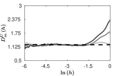
(a)

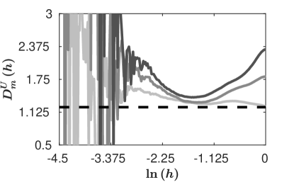
(b)

Figure 3: Henon map: Correlation dimension coarse-grained estimator for $m=\left\{4,6,8\right\}$, the curves for different $m$ values are color-coded in grayscale where the lightest gray corresponds to $m=4$. (a) Noiseless. (b) $\sigma=0.05$. The reported value of the correlation dimension is shown in dashed black line.

2.3 Correlation dimension coarse-grained estimator

Here we present a new coarse-grained estimator for ${D}$ (see Appendix A for deduction) which is given by:

$$\CDu\E{h}= \dot{D}_{m}^{\beta=m}\E{h}+\frac{\Delta_{m}^{\scriptscriptstyle{U}}\E{h}}{1-\Delta_{m}^{\scriptscriptstyle{U}}\E{h}}\bigg{[}\dot{D}_{m}^{\beta=m}\E{h}$$

$$\!+\!2\E{m\!-\!1}\E{\frac{\UCi{m}{\beta=m-2}\E{h}}{\UCi{m}{\beta=m}\E{h}}\!-\!1}\bigg{]}.$$ (8)

The calculation of $\CDu\E{h}$ requires the estimation of $\Delta_{m}^{\scriptscriptstyle{U}}\E{h}$ and two correlation integrals: $\UCi{m}{\beta=m}\E{h}$ and $\UCi{m}{\beta=m-2}\E{h}$. In [24] we have shown that if $\sigma\ll h$, then $\dot{D}_{m}^{\beta=m}\E{h}\to D$. Moreover, under the same condition $\Delta_{m}^{\scriptscriptstyle{U}}\E{h}\to 0$. Replacing in Eq. (8) we have that:

$$\CDu\E{h}\to\dot{D}_{m}^{\beta=m}\E{h}\to D,\quad\text{for}\,\,\sigma\ll h.$$

This means that, in absence of noise, this coarse-grained estimator is the logarithmic derivative of the UCI, which tends to ${D}$. On the other hand, if noise is present, the second term in the right-hand side of Eq. (8) helps to correct the estimation.

Since the GCI is a special case of the UCI for $\beta=2$. The coarse-grained estimator of ${D}$ proposed by Nolte et al. in [22] can be easily derived from Eq. (16) (see Appendix A.1).

In Fig. 3, the estimations of $\CDu\E{h}$ for both a clean and a noisy ($\sigma=0.05$) realizations of the Henon map are shown for $m=\left\{4,6,8\right\}$. In absence of noise, it can be seen in Fig. 3a that the estimator $\CDu\E{h}$ oscillates near the reported value of correlation dimension ($D=1.22$) for a wide range of scales, regardless the value of $m$. In contrast, Fig. 3b shows that $\CDu\E{h}$ overestimates ${D}$. Furthermore, the best estimation is reached with the lowest value of the embedding dimension, $m=4$. This is related with the previously discussed scaling behavior of $\Delta_{m}^{\scriptscriptstyle{U}}\E{h}$. However, it can be observed that the values of $\CDu\E{h}$ are close to the reported value of ${D}$.

(a)

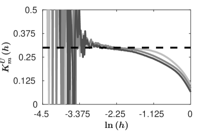
(b)

Figure 4: Correlation entropy coarse-grained estimator for $m=\left\{4,6,8\right\}$, the curves for different $m$ values are color-coded in grayscale where the lightest gray corresponds to $m=4$. (a) Noiseless. (b) $\sigma=0.05$. The reported value of the correlation entropy is shown in dashed black line.

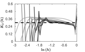
(a)

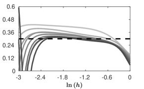
(b)

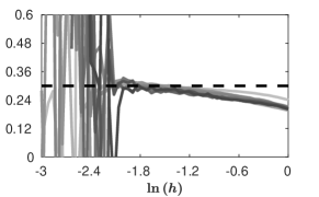
(c)

Figure 5: Henon map with noise ($\sigma=0.05$). Estimation of $K_{2}$ for $m=\left\{4,6,\dots,22\right\}$ through different coarse-grained estimators, the curves for different $m$ values are color-coded in grayscale where the lightest gray corresponds to $m=4$. (a) Jayawardena et al. (b) Nolte et al. (c) $\CKu\E{h}$. The reported value $K=0.3$ is shown in dashed black line.

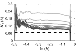
(a)

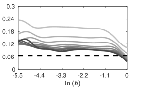
(b)

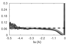
(c)

Figure 6: Rössler system. Estimation of $K_{2}$ for $m=\left\{4,6,\dots,22\right\}$ through different coarse-grained estimators, the curves for different $m$ values are color-coded in grayscale where the lightest gray corresponds to $m=4$. (a) Jayawardena et al. (b) Nolte et al. (c) $\CKu\E{h}$. The reported value $K=0.066$ is shown in dashed black line.

2.4 Correlation entropy coarse-grained estimator

Here proposed coarse-grained entropy estimator is defined as (see Appendix B):

$$\CKu\E{h}= -\frac{1}{2\Delta t\tau}\ln\E{\frac{\UCi{m+2}{\beta=m+2}\E{h}}{\UCi{m}{\beta=m}\E{h}}}$$

$$-\frac{1}{2\Delta t\tau}\ln\E{\frac{\CDu\E{h}}{m}+1}$$

$$+\frac{1}{2\Delta t\tau}\ln\Bigg{[}\Delta_{m}^{\scriptscriptstyle{U}}\E{h}\E{\frac{m\!-\!\dot{D}_{m}^{\beta=m}\E{h}}{m\!-\!\CDu\E{h}}}$$

$$+\E{1\!-\!\Delta_{m}^{\scriptscriptstyle{U}}\E{h}}\E{{\frac{\dot{D}_{m}^{\beta=m}\E{h}}{m}\!+\!1}}\Bigg{]}.$$ (9)

This coarse-grained estimator depends on the correlation integrals $\UCi{m+2}{\beta=m+2}\E{h}$ and $\UCi{m}{\beta=m}\E{h}$, $\Delta_{m}^{\scriptscriptstyle{U}}\E{h}$, the logarithmic derivative $\dot{D}_{m}^{\beta=m}\E{h}$, and the coarse-grained estimator $\CDu\E{h}$. When $\sigma\ll h$ the quantities $\CDu\E{h}\to\dot{D}_{m}^{\beta=m}\E{h}\to D$, and taking into account that for $\sigma\ll h$ [24]:

$$\frac{1}{2\Delta t\tau}\ln\left[\frac{\UCi{m+2}{\beta=m+2}\E{h}}{\UCi{m}{\beta=m}\E{h}}\right]\approx\frac{1}{2\Delta t\tau}\ln\E{\frac{D}{m}+1}-K_{2},$$

then it can be easily shown that:

$$\CKu\E{h}\to K_{2},\quad\text{for}\quad\sigma\ll h\quad\text{and}\quad m\gg D.$$

The estimations of $\CKu\E{h}$ from both a clean and a noisy realization ($\sigma=0.05$) of the Henon map for $m=\left\{4,6,8\right\}$ are presented in Fig. 4. It can be observed that in both cases (Fig. 4a, Fig. 4b) $\CKu\E{h}$ is near to the reported value of $K_{2}=0.3$ for all $m$ values. This is the main advantage of the UCI in comparison with other correlation integrals [24].

The last statement can be confirmed by comparing $\CKu\E{h}$ with two similar coarse-grained estimators based on different correlation integrals. The first one was proposed by Jayawardena et al. [17], and it is based on the Grassberger and Procaccia correlation integral ($C_{m}\E{h}$). The second one was proposed by Nolte et al., and it is calculated from the GCI ($T_{m}\E{h}$). These approaches, as well as the here proposed, $\CKu\E{h}$ only requires the estimation of two correlation integrals of the same kind.

In Fig. 5, the estimations of ${K_{2}}$ for the Henon map through the estimators proposed by Jayawardena et al., Nolte et al. and $\CKu\E{h}$ can be compared. They were calculated from a time series of length $N=5000$ with added white Gaussian noise at a level $\sigma=0.05$. The correlation sums $C_{m}\E{h}$, $T_{m}\E{h}$, $\UCi{m}{\beta=m}\E{h}$ and $\UCi{m}{\beta=m-2}\E{h}$ were calculated for $m=\{4,6,\dots,22\}$ with $\tau=1$. Figure 5a shows the results for the estimator proposed by Jayawardena et al. It can be observed that, as $m$ is increased, this estimator slowly approaches to the reported value of ${K_{2}}$. However, it must be pointed out that, regardless that the dimension of this map is low ($D=1.22$), high values of $m$ are needed in order to converge. On the other hand, it can be seen in Fig. 5b that the results of the coarse-grained estimator proposed by Nolte et al. also converge slowly to the reported value for ${K_{2}}$. In contrast, in Fig. 5c it can be observed that the estimator $\CKu\E{h}$ approaches faster to the value of ${K_{2}}$ than the other two studied estimators. Note that the curves for different $m$ values of $\CKu\E{h}$ are very close to each other, meaning that this estimator is more robust to changes in the parameter $m$. Please note that the curves corresponding to $m=\left\{4,6,8\right\}$ of Fig. 5c are also shown in Fig. 4b.

The same methodology was applied to a clean time series obtained from the Rössler system:

$$\begin{cases}\dot{x}&=-y-z\\ \dot{y}&=x+ay\\ \dot{z}&=b+z\E{x-c}\end{cases},$$

where $a=0.15$, $b=0.2$ and $c=10$. The system was solved using the Runge-Kutta method with time step $0.5$ and initial condition $x\E{0}=0.1$, $y\E{0}=0.1$, $z\E{0}=0.1$. The first $20000$ data points were discarded, and the next $N=10000$ data points were taken to estimate the attractor’s invariants. The correlation sums $C_{m}\E{h}$, $T_{m}\E{h}$, $\UCi{m}{\beta=m}\E{h}$ and $\UCi{m}{\beta=m-2}\E{h}$ were calculated for $m=\left\{4,6,\dots,22\right\}$ with $\tau=3$.

The results for the estimators proposed by Jayawardena, Nolte, and $\CKu\E{h}$ are shown in Figs. 6a, 6b and 6c, respectively. In all three cases, a typical scaling behavior can be observed. Once again, the estimators proposed by Jayawardena and Nolte need high values of $m$, in contrast with $\CKu\E{h}$. Interestingly, all estimators converge to values of correlation entropy that differs from the one reported ($K_{2}=0.066$) [6]. Both the Jayawardena’s and Nolte’s estimators converge to $\hat{K}_{2}\approx 0.085$, while $\CKu\E{h}$ converges to $\hat{K}_{2}\approx 0.052$. From these results, we can conclude that the estimator $\CKu\E{h}$ converges by using low values of $m$, in comparison with the previously proposed estimators [22, 17].

3 Automatic invariants estimation

In practical applications, it is important to verify the existence of a scaling behavior for a range of $h$. The determination of a stable scaling region, which is required to estimate the invariants, is usually done by visual inspection. However, that is not feasible when large sets of data are studied Additionally, the subjective judgment should be avoided. The necessity of an algorithm for the automatic estimation of invariants arises, once the scaling regime has been confirmed. In this section, we propose an algorithm (see algorithm 2) based on the coarse-grained estimators $\CSu\E{h}$, $\CDu\E{h}$ and $\CKu\E{h}$, that is able to automatically estimate these invariants. Before describing this algorithm, we need to detail some aspects about the calculation of the U-correlation integral.

3.1 Noise-assisted correlation algorithm

Figure 7: Noise-assisted correlation algorithm. The $\omega$-th comparator ($\omega=1,2,\dots,\Omega$) with threshold ${\theta_{\omega}=0}$ receives as input the squared distance between two $m$-dimensional delay vectors minus an i.i.d. realization $\alpha_{\omega}\leavevmode\nobreak\ \sim\E{h^{2}/2}\inlineChiS$. All binary outputs $\mu_{\omega}$ are averaged to calculate the U-correlation sum $\widehat{U}_{m}^{\beta}\E{h}$.

The UCI is approximated with U-correlation sum $\widehat{U}_{m}^{\beta}\!\E{h}$. The calculation of $\widehat{U}_{m}^{\beta}\!\E{h}$ requires a computationally expensive numerical integration due to the kernel of the UCI. However, we can use the noise-assisted correlation algorithm instead [24] (see Fig. 7). This algorithm begins by calculating the squared distances between each pair of delay vectors $z_{\omega}=\norm{\bm{x_{i}}-\bm{x_{j}}}^{2}$, where $\omega=\{\left(i,j\right)/\,\,\,i=1,2,\dots L,\,\,j=1,2,\dots,L,\,\,\,i\neq j\}$ and $\Omega=L\E{L-1}$. Then, for each squared distance $z_{\omega}$ an i.i.d. noise realization $\alpha_{\omega}\sim\text{Gamma}\E{\beta/2,h^{2}}$ is subtracted. Here, $\beta/2$ and $h^{2}$ are the shape and scale parameters, respectively. The result is then compared with a threshold $\theta_{\omega}=0$ to produce a binary output $u_{\omega}$. Then $\widehat{U}_{m}^{\beta}\!\E{h}$ is the average of all binary outputs. These steps must be repeated for each value of $h$ and $m$. Algorithm 1 describes all the steps that must be followed in order to estimate the noise-assisted U-correlation sum. The noise realizations $\alpha_{\omega}$ were generated using $\inlineChiS$ realizations given that, if $X\sim\inlineChiS$, then $\E{h^{2}/2}X\sim\text{Gamma}\E{\beta/2,h^{2}}$.

As an example, the correlation integral $\UCi{m}{\beta=m}\E{h}$ can be approximated by $\widehat{U}_{m}^{\beta=m}\!\E{h}$ which in turn is calculated from the squared distances $z_{\omega}$ of $m$-dimensional delay vectors, and noise realizations $\alpha_{\omega}$ that follow a Gamma distribution with shape parameter equal to $m/2$. Similarly, the correlation sum $\widehat{U}_{m+2}^{\beta=m-2}\!\E{h}$ can be obtained from the squared distances $z_{\omega}$ of $(m+2)$-dimensional delay vectors and noise realizations $\alpha_{\omega}$ following a Gamma distribution with shape parameter equal to $m/2-1$.

Algorithm 1 Noise-assisted U-correlation algorithm.

1: Form the $m$-dimensional delay vectors from the temporal series and calculate all pairwise squared distances $z_{\omega}$ with $1\leq\omega\leq\Omega=L\E{L-1}$.

2: Fix the value of the parameter $h$ and obtain $\Omega$ realization of noise $\alpha_{\omega}$ from the distribution $\E{h^{2}/2}\inlineChiS$.

3: Calculate the binary variable:

$$u_{\omega}\E{h}=\begin{cases}0&\text{if}\quad z_{\omega}-\alpha_{\omega}\geq 0\\ 1&\text{otherwise}\end{cases}.$$

4: Calculate the U-correlation sum as:

$$\widehat{U}_{m}^{\beta}\E{h}=\frac{1}{\Omega}\sum_{\omega=1}^{\Omega}{u_{\omega}}.$$

5: Repeat steps $1$-$4$ for all values of $h$ and $m$.

3.2 Algorithm for automatic estimation of invariants

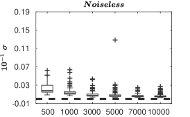
(a)

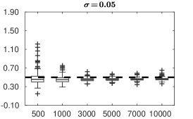
(b)

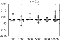
(c)

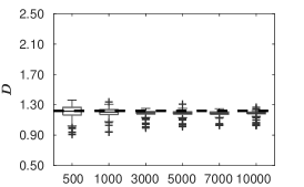
(d)

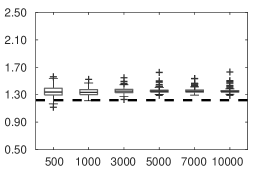
(e)

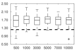
(f)

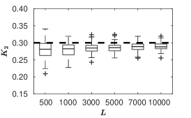
(g)

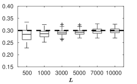
(h)

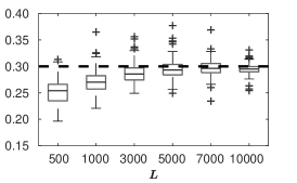
(i)

Figure 8: Henon map. Box plot of the estimation of $\sigma$, $D$, and $K_{2}$ for different numbers of available delay vectors ${L=\left\{500,1000,3000,5000,10000\right\}}$. First row: estimation of $\sigma$. (a) noiseless, (b) $\sigma=0.05$, and (c) $\sigma=0.2$. Second row: estimation of $D$. (d) noiseless, (e) $\sigma=0.05$, and (f) $\sigma=0.2$. Third row: estimation of $K_{2}$. (g) noiseless, (h) $\sigma=0.05$, and (i) $\sigma=0.2$. The reported values are shown in dashed black line.

The automatic algorithm to estimate invariants begins by approximating the U-correlation integrals $\UCi{m}{\beta=m}\E{h}$ and $\UCi{m}{\beta=m-2}\E{h}$, for different $m$ values ($m>2$) using the noise-assisted correlation algorithm (Alg. 1). This step does not requires a narrow range of $h$ as initial guess. For example, for a normalized time series the range $10^{-8}\leq h\leq 10$ is a good choice. On the other hand, note that the expression $\UCi{m}{\beta=m-2}\E{h}$ requires values of $m>2$ since Gamma distribution’s shape parameter must be greater than zero.

Next, the logarithmic derivatives $\dot{D}_{m}^{\beta=m}\E{h}$, $\dot{D}^{\beta=m}_{m+2}\E{h}$ are computed and $\Delta_{m}^{\scriptscriptstyle{U}}\E{h}$ is calculated using Eq. (6). To calculate the logarithmic derivatives, we make use of a wavelet transform approach to approximate the derivative [21]. This allows us to achieve better estimations of the invariants because it implements a low-pass filter reducing the high-frequency oscillations that are naturally present in estimators derived from the noise-assisted algorithm [24]. Please observe that correlation integral $\UCi{m+2}{\beta=m}\E{h}$ is equal to $\UCi{\hat{m}}{\beta=\hat{m}-2}\E{h}$ correlation integral evaluated at $\hat{m}=m+2$. In order to obtain ${\sigma}$, the coarse-grained estimator $\CSu\E{h}$ must be calculated [Eq. (7)].

To obtain a suitable range of scale values where the invariants can be estimated, one must look for a range of $h$ where the coarse-grained estimator is nearly constant and its variation across the different $m$ values is the smallest. In this sense, for the noise level we define the functions:

$$A_{\sigma}\E{h}= \frac{1}{M}\sum_{i=1}^{M}{\frac{\text{d}\,\sigma^{U}_{m_{i}}\E{h}}{\text{d}\ln h}},$$

$$V_{\sigma}\E{h}= \frac{1}{M-1}\sum_{i=1}^{M}{\E{\sigma^{U}_{m_{i}}\E{h}-\hat{\sigma}^{U}\E{h}}^{2}},$$

and

$$F_{\sigma}\E{h}= A_{\sigma}\E{h}V_{\sigma}\E{h},$$

where $m\in\left\{m_{1},m_{2},\dots,m_{i},\dots,m_{M}\right\}$, $\hat{\sigma}^{U}\E{h}$ is the average of $\CSu\E{h}$ across $m$. $A_{\sigma}\E{h}$ is the average over $m$ of the derivative of $\CSu\E{h}$ with respect to $\ln h$, $V_{\sigma}$ gives the variation of $\CSu\E{h}$ across $m$ and $F_{\sigma}\E{h}$ is the product of the aforementioned functions. We propose to estimate ${\sigma}$ within a range of $h$ centered at the $h$ value at which $F_{\sigma}\E{h}$ is minimum. In this way, ${\sigma}$ is estimated in a range of $h$ centered in a plateaued region (scaling region) of $\CSu\E{h}$, and its value is consistent through the parameter $m$.

The correlation dimension is determined using the coarse-grained estimator $\CDu\E{h}$ [Eq. (8)]. To find a range of $h$ values to estimate ${D}$, we define the functions $A_{D}\E{h}$, $V_{D}\E{h}$ and $F_{D}\E{h}$ similarly to the ones above but using the estimator $\CDu\E{h}$ instead of $\CSu\E{h}$. The estimation of ${D}$ must be done within a range of $h$ centered at the $h$ value at which $F_{D}\E{h}$ is minimum.

Finally, the correlation entropy can be estimated using the coarse-grained estimator $\CKu\E{h}$. As it can be seen in Eq. (9), this estimator depends on $\Delta_{m}^{\scriptscriptstyle{U}}\E{h}$, $\dot{D}_{m}^{\beta=m}\E{h}$, the coarse-grained estimator $\CDu\E{h}$ and the ratio between $\UCi{m}{\beta=m}\E{h}$ and $\UCi{m+2}{\beta=m+2}\E{h}$. ${K_{2}}$ must be determined within a range of $h$ centered at the $h$ value at which $F_{K_{2}}\E{h}$ is minimum.

Algorithm 2 Automatic estimation of attractors’ invariants.

1: Calculate $\UCi{m}{\beta=m}\E{h}$ and $\UCi{m}{\beta=m-2}\E{h}$ using Alg. 1 for $m>2$.

2: Calculate $\Delta_{m}^{\scriptscriptstyle{U}}\E{h}$ using Eq. (6) and the UCI obtained in step $1$.

3: Compute $\CSu\E{h}$ with Eq. (7) and obtain the function $F_{\sigma}\E{h}$. Estimate $\sigma$ within a range of $h$ centered at the value $h$ where $F_{\sigma}\E{h}$ is minimum.

4: Use $\UCi{m}{\beta=m}\E{h}$, $\UCi{m}{\beta=m-2}\E{h}$ and $\Delta_{m}^{\scriptscriptstyle{U}}\E{h}$ to calculate $\CDu\E{h}$ (Eq. (8)) and obtain the function $F_{D}\E{h}$. Estimate $D$ within a range of $h$ centered at the value $h$ where $F_{D}\E{h}$ is minimum.

5: Obtain $\CKu\E{h}$ (Eq. (9)) using $\UCi{m}{\beta=m}\E{h}$, $\Delta_{m}^{\scriptscriptstyle{U}}\E{h}$ and $\CDu\E{h}$. Calculate the function $F_{K_{2}}\E{h}$. Estimate $K_{2}$ within a range of $h$ centered at the value $h$ where $F_{D}\E{h}$ is minimum.

3.3 Simulations

The aforementioned methodology was applied to a set of $128$ realization of the Henon map with different noise levels ${\sigma=\left\{0,0.05,0.2\right\}}$ and data lengths which are proportional to the number $L$ of available delay vectors to estimate the invariants ${\sigma}$, ${D}$ and ${K_{2}}$. To calculate the UCI s for ${m=\left\{4,5,\dots,8\right\}}$ all realizations were normalized (unitary standard deviation), and the nearest $15$ temporal neighbors of each delay vector were discarded [19].

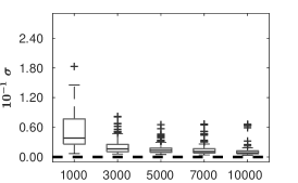
(a)

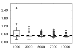
(b)

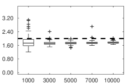
(c)

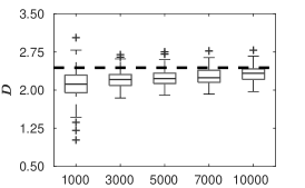
(d)

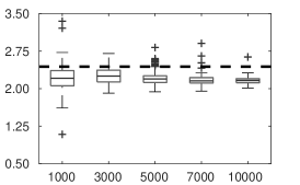
(e)

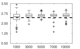
(f)

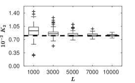
(g)

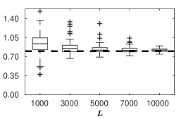
(h)

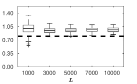
(i)

Figure 9: Mackey-Glass box plot of the estimation of $\sigma$, $D$, and $K_{2}$ for different numbers of available delay vectors, ${L=\left\{1000,3000,5000,10000\right\}}$. First row: estimation of $\sigma$. (a) noiseless, (b) $\sigma=0.05$, and (c) $\sigma=0.2$. Second row: estimation of $D$. (d) noiseless, (e) $\sigma=0.05$, and (f) $\sigma=0.2$. Third row: estimation of $K_{2}$. (g) noiseless, (h) $\sigma=0.05$, and (i) $\sigma=0.2$. The reported values are shown in dashed black line.

Figure 8 shows the boxplots of the invariants ${\sigma}$, ${D}$ and ${K_{2}}$ for $L=\left\{500,1000,3000,5000,10000\right\}$. Unfortunately, there is no other automatic algorithm for the estimation of invariants. Due to this reason, we only can compare the results of our estimations with previously reported values calculated by selecting the scaling range by visual inspection. For the noise level estimation (first row of Fig. 8), it can be observed that, in absence of noise, our algorithm overestimates the value of ${\sigma}$ (dashed black line). On the contrary, for higher noise levels ($\sigma=\left\{0.05,0.2\right\}$) the proposed method slightly underestimates ${\sigma}$. It can be noticed that, regardless the noise level, the median of each box is very close to the true value of ${\sigma}$ and the variance of the estimation decreases as the number of data points increases. The estimation of the correlation dimension is shown in the second row of Fig. 8. It can be seen in Fig. 8d that for noiseless time series the estimation of ${D}$ is very close to the reported value ($D=1.22$) and its variance decreases as the length of the time series is increased. For higher noise levels, the correlation dimension is slightly biased, but the estimations are still close to the previously reported value.

The results for the correlation entropy are shown in the third row of Fig. 8. In general, the here proposed method yields correlation entropy values converging to values lesser than the reported for this map ($K_{2}=0.3$).

The proposed approach was also tested on the Mackey-Glass time series, which is generated by the following nonlinear time-delay differential equation:

$$\dot{x}\E{t}=\frac{ax\E{t-\lambda}}{1+\left[x\E{t-\lambda}\right]^{10}}-bx\E{t},$$

where $a=0.2$, $b=0.1$, and $\lambda=23$. We estimate the invariants $\sigma$, $D$, and $K_{2}$ from $128$ realizations with different initial conditions and normalized to have unitary standard deviation. The embedding dimensions were $m=\left\{4,6,\dots,10\right\}$ and the embedding lag $\tau$ was set to the first local minimum of the mutual information function ($\tau=20$) [18]. Finally, the nearest $15$ temporal neighbors of each delay vector were discarded.

The results of these simulations are presented in Fig. 9 and the estimations of the noise level are presented in Figs. 9a, 9b and 9c. In absence of noise the algorithm estimates small positive values of ${\sigma}$. This behavior is explained because the function $\Delta_{m}^{\scriptscriptstyle{U}}\E{h}$ tends to zero as the length of the time series increases, producing more accurate estimations with less variance. In presence of noise ($\sigma=0.05$ and $\sigma=0.2$) the here proposed algorithm underestimates the noise level, but in Fig.8 it can be seen how the median values tend to the real value of ${\sigma}$ as $L$ increases.

The estimations of the correlation dimension are shown in the second row of Fig. 9. For clean time series, our algorithm provides estimations of ${D}$ very close to the reported value $D=2.44$ [13]. As the data length is increased, the estimations approach the reported value. In case of noisy time series, the estimations of the correlation dimension are greater than those obtained in the noiseless case. Nevertheless, the estimation of ${D}$ is still very good.

In Figs. 9g, 9h and 9i the estimations for the correlation entropy are presented. Our algorithm achieves satisfactory estimations of ${K_{2}}$ (reported value $K_{2}=0.008$) [14], even in presence of noise. It can be observed that regardless the value of $L$ the estimation of $K_{2}$ is consistent, but its variance decreases as the data length increases.

4 Discussion

In this section, we review the main contributions of this article and give some practical recommendations for its implementation. In this work, we introduce a new methodology to estimate the correlation dimension, the correlation entropy and the noise level of time series. This approach is based on the recent proposed U-correlation integral (Eq. (3)), introduced in [24], which uses a kernel function that depends on the embedding dimension. From the scaling function of the UCI (Eq. (5)), we have developed a set of coarse-grained estimators for the correlation dimension (Eq. (8)), the correlation entropy (Eq. (9)) and the noise level (Eq. (7)). The advantage of these coarse-grained estimators is that they only depend on the estimation of two U-correlation integrals. In other words, they do not need of the tuning of any external parameter and/or the estimation of the noise level, as it does other approaches [6, 16, 24].

From the results presented in the previous section, we can conclude that the here proposed algorithm (Alg. 2) is able to automatically select the scaling region and to estimate the invariants. As far as we know, there is no other algorithms with these features reported in the literature. For this reason, our results were compared against reported estimations that were obtained selecting the scaling region by visual inspection.

Regarding the coarse-grained estimators, the most outstanding result was obtained with $\CKu\E{h}$. It is more accurate than previously proposed estimators and needs lesser values of $m$ to converge.

Finally, it is important to recall that the implementation of our method only requires the calculation of two correlation integrals: $\UCi{m}{\beta=m}\E{h}$ and $\UCi{m}{\beta=m-2}\E{h}$, that can be obtained through the noise-assisted correlation algorithm (Alg. 1). It is also important to say that the time series must be normalized to have unitary standard deviation. As it was reported in [24], the correlation integrals computed using the noise-assisted correlation algorithm present oscillations for small values of $h$. This phenomenon makes difficult to look for scaling regions over small $h$ values. In order to avoid this difficulty three strategies can be followed: The first one is to increase the number of comparators $\Omega$ in the noise-assisted correlation algorithm by increasing the data length. This will make coarse-grained curves smoother and also will improve the convergence of these estimators. The second one is to increase $\Omega$ by making copies of the squared distances between delay vectors $z_{\omega}$ and adding different noise realizations $\mu_{\omega}$ to them. This will not improve the convergence of any coarse-grained estimators to the invariant since no new information is added, but the ripple in the coarse-grained curves will be reduced. The third one, and the one we have found as the more adequate, is to use the algorithm proposed in [21] to calculate the logarithmic derivatives of the UCI. This algorithm calculates a smoothed version of the derivative of a function using the wavelet transform.

5 Conclusions

The original contributions of this document are twofold: both a new method for the estimation of invariants based on the recently proposed U-correlation integral, and an algorithm for the automatic selection of the scaling region. The combined use of these two ideas allows to automatically estimate the noise level, correlation dimension and correlation entropy of a dynamical system. This approach have been statistically tested using synthetic data coming from low-dimensional systems with different data lengths and noise levels. The results suggest that our algorithm provides robust estimations of the correlation dimension, the correlation entropy and the noise level.

Appendix A Analytic deduction for the coarse-grained $D$ estimator

Let:

$$a=\frac{\beta+m}{2}; b=\frac{m-D}{2}; c=\frac{m+2}{2};$$

$$y=-\frac{h^{2}}{4\sigma^{2}}; \frac{\,\text{d}y}{\,\text{d}h}=-\frac{h}{2\sigma^{2}},$$ (10)

and

$$P=\E{-1}^{m/2}\frac{\hat{\phi}}{2}e^{{{-m\Delta t\tau K_{2}}\mathord{\vphantom{-m\Delta t\tau K_{2}}\kern-1.2pt}}}\frac{\Gf{D/2}\Gf{\E{\beta\!+\!m}/{2}}}{\Gf{\beta/2}\Gf{m/2\!+\!1}}$$

then Eq. (5) can be rewritten as:

$$\UCi{m}{\beta}\E{y}=Py^{m/2}\HF{a}{b}{c}{y}$$ (11)

We need to find the logarithmic derivative of Eq. (11). For this end we can find its first derivative as:

$${\frac{\text{d}\left[\UCi{m}{\beta}\E{y}\right]}{\text{d}h}}= {\frac{\text{d}\left[Py^{m/2}\HF{a}{b}{c}{y}\right]}{\text{d}y}}{\frac{\text{d}y}{\text{d}h}}$$

using Eq. 15.2.1 from Ref. [1]:

$${\frac{\text{d}\left[\UCi{m}{\beta}\E{y}\right]}{\text{d}h}}= -\frac{Ph}{2\sigma^{2}}y^{m/2}\bigg{[}\frac{m}{2}\HF{a}{b}{c}{y}$$

$$+\frac{ab}{c}\HF{a\!+\!1}{b\!+\!1}{c\!+\!1}{y}\bigg{]}$$

Then the logarithmic derivative can be found as:

$${\frac{\text{d}\left[\ln\UCi{m}{\beta}\E{y}\right]}{\text{d}\ln h}}= \frac{h}{{\UCi{m}{\beta}\E{y}}}{{\frac{\text{d}\UCi{m}{\beta}\E{y}}{\text{d}h}}}$$

$$= m+\frac{2aby}{c}\frac{\HF{a+1}{b+1}{c+1}{y}}{\HF{a}{b}{c}{y}},$$ (12)

and for simplicity in the notation:

$$\dot{D}_{m}^{\beta}\E{y}={\frac{\text{d}\left[\ln\UCi{m}{\beta}\E{y}\right]}{\text{d}\ln h}}.$$

Using the identity [10, Eq. 9.137.9]:

$$\frac{aby}{c}\HF{a\!+\!1}{b\!+\!1}{c\!+\!1}{y}= \frac{1}{1\!-\!y}\big{[}\E{c\!-\!a}\HF{a\!-\!1}{b}{c}{y}$$

$$+\E{a\!-\!c\!+\!by}\HF{a}{b}{c}{y}\big{]}$$ (13)

we can rewrite Eq. (12) as:

$$\dot{D}_{m}^{\beta}\E{y}= m+\frac{2}{1\!-\!y}\left[\E{a\!-\!c\!+\!by}+\E{c\!-\!a}\frac{\HF{a\!-\!1}{b}{c}{y}}{\HF{a}{b}{c}{y}}\right]$$ (14)

From Eq. (5) and using the definitions in (10) it is possible to demonstrate that:

$$\frac{\UCi{m}{\beta-2}\E{y}}{\UCi{m}{\beta}\E{y}}=\frac{\beta-2}{2\E{a-1}}\frac{\HF{a-1}{b}{c}{y}}{\HF{a}{b}{c}{y}}.$$ (15)

Substituting Eq. (15) into (14):

$$\dot{D}_{m}^{\beta}\E{y}= m+\frac{2}{1\!-\!y}\left[\E{a\!-\!c\!+\!by}+\frac{2\E{c\!-\!a}\E{a\!-\!1}}{\beta\!-\!2}\frac{\UCi{m}{\beta-2}\E{y}}{\UCi{m}{\beta}\E{y}}\right]$$

Restoring the values of $\beta$, $m$ and $D$ and clearing for $D$

$$D= \dot{D}_{m}^{\beta}\E{y}\!-\!\frac{1}{y}\left[\dot{D}_{m}^{\beta}\E{y}\!+\!\E{m\!+\!\beta\!-\!2}\E{\frac{\UCi{m}{\beta-2}\E{y}}{\UCi{m}{\beta}\E{y}}\!-\!1}\right]$$

notice that $-1/y=4\sigma^{2}/h^{2}$ and from Eq. (6)

$$\frac{h^{2}}{4\sigma^{2}}=\frac{\Delta_{m}^{\scriptscriptstyle{U}}\E{h}}{1-\Delta_{m}^{\scriptscriptstyle{U}}\E{h}},$$

then

$$D= \dot{D}_{m}^{\beta}\E{h}+\frac{\Delta_{m}^{\scriptscriptstyle{U}}\E{h}}{1-\Delta_{m}^{\scriptscriptstyle{U}}\E{h}}\bigg{[}\dot{D}_{m}^{\beta}\E{h}$$

$$\!+\!\E{m\!+\!\beta\!-\!2}\E{\frac{\UCi{m}{\beta-2}\E{h}}{\UCi{m}{\beta}\E{h}}\!-\!1}\bigg{]}.$$ (16)

Making $\beta=m$, the coarse-grained estimator for $D$ can be defined as:

$$\CDu\E{h}= \dot{D}_{m}^{\beta=m}\E{h}+\frac{\Delta_{m}^{\scriptscriptstyle{U}}\E{h}}{1-\Delta_{m}^{\scriptscriptstyle{U}}\E{h}}\bigg{[}\dot{D}_{m}^{\beta=m}\E{h}$$

$$\!+\!2\E{m\!-\!1}\E{\frac{\UCi{m}{\beta=m-2}\E{h}}{\UCi{m}{\beta=m}\E{h}}\!-\!1}\bigg{]}.$$ (17)

A.1 Relation with Nolte’s et al. coarse-grained $D$ estimator:

It was proved in [24] that the Gaussian correlation integral is a particular case of the U-correlation integral that arises when $\beta$ is constant and equal to $2$. Let $\beta=2$, then from Eq. (15) it can be proved that:

$$\frac{\UCi{m}{\beta-2}\E{h}}{\UCi{m}{\beta}\E{h}}=0,$$

for all $m$ values. Thus, Eq. (16) can be rewritten as:

$$D= \dot{D}^{\beta=2}_{m}\E{h}-\frac{\Delta_{m}^{\scriptscriptstyle{U}}\E{h}}{1-\Delta_{m}^{\scriptscriptstyle{U}}\E{h}}\E{m-\dot{D}^{\beta=2}_{m}\E{h}}.$$ (18)

Finally, given that the Gaussian correlation integral is a particular case of the U-correlation integral for $\beta=2$, i.e., ${\UCi{m}{\beta=2}\E{h}=T_{m}\E{h}}$, we can write:

$$\dot{D}^{\beta=2}_{m}\E{h}={\frac{\text{d}\left[\ln T_{m}\E{h}\right]}{\text{d}\ln h}}.$$

Then, Eq. (18) is the same coarse-grained estimator for the correlation dimension that was derived by Nolte et al. in [22].

Appendix B Analytic deduction for the coarse-grained $K_{2}$ estimator

The analytic deduction of the coarse-grained estimator for ${K_{2}}$ begins by defining the quantity:

$$M=\frac{\hat{\phi}}{2}\E{2\sigma^{2}}^{D}\Gf{D/2}.$$

Substituting this equation and Eq. (10) into Eq. (5) we can write:

$$\UCi{m}{\beta}\E{y}=M\frac{\Gf{a}}{\Gf{\beta/2}\Gf{c}}e^{{{-m\Delta t\tau K_{2}}\mathord{\vphantom{-m\Delta t\tau K_{2}}\kern-1.2pt}}}\E{-y}^{m/2}\HF{a}{b}{c}{y}$$

Then the ratio $\UCi{m+2}{\beta+2}\E{y}/\UCi{m}{\beta}\E{y}$ can be written as:

$$\frac{\UCi{m+2}{\beta+2}\E{y}}{\UCi{m}{\beta}\E{y}}=\frac{2a\E{a\!+\!1}}{\beta c}e^{{{-2\Delta t\tau K_{2}}\mathord{\vphantom{-2\Delta t\tau K_{2}}\kern-1.2pt}}}\E{-y}\frac{\HF{a\!+\!2}{b\!+\!1}{c\!+\!1}{y}}{\HF{a}{b}{c}{y}}.$$

Making $\alpha=a+1$:

$$\frac{\UCi{m+2}{\beta+2}\E{y}}{\UCi{m}{\beta}\E{y}}=\frac{2\E{\alpha\!-\!1}\alpha}{\beta c}e^{{{-2\Delta t\tau K_{2}}\mathord{\vphantom{-2\Delta t\tau K_{2}}\kern-1.2pt}}}\E{-y}\frac{\HF{\alpha\!+\!1}{b\!+\!1}{c\!+\!1}{y}}{\HF{\alpha\!-\!1}{b}{c}{y}}.$$ (19)

The identity in Eq. (13) can be rewritten as:

$$\frac{\alpha\E{-y}}{c}\frac{\HF{\alpha\!+\!1}{b\!+\!1}{c\!+\!1}{y}}{\HF{\alpha\!-\!1}{b}{c}{y}}= \frac{-1}{b\E{1\!-\!y}}\bigg{[}\E{c\!-\!\alpha}$$

$$+\E{\alpha\!-\!c\!+\!by}\frac{\HF{\alpha}{b}{c}{y}}{\HF{\alpha\!-\!1}{b}{c}{y}}\bigg{]}.$$ (20)

Substituting Eq. (20) into Eq. (19) and restituting $a$:

$$\frac{\UCi{m+2}{\beta+2}\E{y}}{\UCi{m}{\beta}\E{y}}= \frac{-2a}{\beta b\E{1-y}}e^{{{-2\Delta t\tau K_{2}}\mathord{\vphantom{-2\Delta t\tau K_{2}}\kern-1.2pt}}}\bigg{[}\E{c\!-\!a\!-\!1}+$$

$$+\E{a\!+\!1\!-\!c\!+\!by}\frac{\HF{a\!+\!1}{b}{c}{y}}{\HF{a}{b}{c}{y}}\bigg{]}.$$ (21)

Using the identity [10, Eq. 9.137.12]:

$$\frac{by}{c}\frac{\HF{a+1}{b+1}{c+1}{y}}{\HF{a}{b}{c}{y}}+1=\frac{\HF{a+1}{b}{c}{y}}{\HF{a}{b}{c}{y}}.$$ (22)

Equation (21) can be written as:

$$\frac{\UCi{m+2}{\beta+2}\E{y}}{\UCi{m}{\beta}\E{y}}= \frac{e^{{{-2K_{2}\Delta t\tau}\mathord{\vphantom{-2K_{2}\Delta t\tau}\kern-1.2pt}}}}{2b\beta\E{y-1}}\bigg{[}4a\E{c\!-\!a\!-\!1}+$$

$$+2\E{a\!+\!1\!-\!c\!+\!by}\E{\frac{2aby}{c}\frac{\HF{a\!+\!1}{b\!+\!1}{c\!+\!1}{y}}{\HF{a}{b}{c}{y}}+2a}\bigg{]}.$$ (23)

Using Eq. (14)

$$\frac{\UCi{m+2}{\beta+2}\E{y}}{\UCi{m}{\beta}\E{y}}= \frac{e^{{{-2K_{2}\Delta t\tau}\mathord{\vphantom{-2K_{2}\Delta t\tau}\kern-1.2pt}}}}{2b\beta\E{y-1}}\bigg{[}4a\E{c\!-\!a\!-\!1}+$$

$$+2\E{a\!+\!1\!-\!c\!+\!by}\E{\dot{D}_{m}^{\beta}\E{y}-m+2a}\bigg{]}.$$ (24)

Replacing the values of $a$, $c$ and $b$:

$$\frac{\UCi{m+2}{\beta+2}\E{y}}{\UCi{m}{\beta}\E{y}}= \frac{e^{{{-2K_{2}\Delta t\tau}\mathord{\vphantom{-2K_{2}\Delta t\tau}\kern-1.2pt}}}}{2b\beta\E{y\!-\!1}}\left[\!-\!\beta\E{m\!+\!\beta}\!+\!\E{\beta\!+\!2by}\E{\dot{D}_{m}^{\beta}\E{y}\!+\!\beta}\right]$$

$$= \frac{e^{{{-2K_{2}\Delta t\tau}\mathord{\vphantom{-2K_{2}\Delta t\tau}\kern-1.2pt}}}}{2b\E{y\!-\!1}}\bigg{[}\dot{D}_{m}^{\beta}\E{y}\!-\!m\!+\!{2by}\E{{\frac{\dot{D}_{m}^{\beta}\E{y}}{\beta}\!+\!1}}\bigg{]}$$

$$= \frac{e^{{{-2K_{2}\Delta t\tau}\mathord{\vphantom{-2K_{2}\Delta t\tau}\kern-1.2pt}}}}{\E{y\!-\!1}}\left[\frac{\dot{D}_{m}^{\beta}\E{y}\!-\!m}{m\!-\!D}+y\E{{\frac{\dot{D}_{m}^{\beta}\E{y}}{\beta}\!+\!1}}\right].$$ (25)

It can be shown that $\Delta_{m}^{\scriptscriptstyle{U}}\E{h}=1/\E{1-y}$ and $1-\Delta_{m}^{\scriptscriptstyle{U}}\E{h}=y/\E{y-1}$ so:

$$\frac{\UCi{m+2}{\beta+2}\E{y}}{\UCi{m}{\beta}\E{y}}= e^{{{-2K_{2}\Delta t\tau}\mathord{\vphantom{-2K_{2}\Delta t\tau}\kern-1.2pt}}}\Bigg{[}\Delta_{m}^{\scriptscriptstyle{U}}\E{h}\E{\frac{m\!-\!\dot{D}_{m}^{\beta}\E{y}}{m\!-\!D}}+$$

$$+ \E{1\!-\!\Delta_{m}^{\scriptscriptstyle{U}}\E{h}}\E{{\frac{\dot{D}_{m}^{\beta}\E{y}}{\beta}\!+\!1}}\Bigg{]}.$$

Taking natural logarithm, subtracting the term $\ln\E{D/\beta+1}$ on both sides and dividing by $2\Delta t\tau$:

$$K_{2}-\frac{1}{2\Delta t\tau}\ln\E{\frac{D}{\beta}+1}= \frac{1}{2\Delta t\tau}\Bigg{\{}\ln\Bigg{[}\Delta_{m}^{\scriptscriptstyle{U}}\E{h}\E{\frac{m\!-\!\dot{D}_{m}^{\beta}\E{y}}{m\!-\!D}}+$$

$$+ \E{1\!-\!\Delta_{m}^{\scriptscriptstyle{U}}\E{h}}\E{{\frac{\dot{D}_{m}^{\beta}\E{y}}{\beta}\!+\!1}}\Bigg{]}$$

$$- \ln\left[\frac{\UCi{m+2}{\beta+2}\E{y}}{\UCi{m}{\beta}\E{y}}\right]-\ln\E{\frac{D}{\beta+1}}\Bigg{\}}.$$ (26)

Let call the left-hand side of Eq. (26) as $\CKu\E{h}$:

$$\CKu\E{h}= \frac{1}{2\Delta t\tau}\Bigg{\{}\ln\Bigg{[}\Delta_{m}^{\scriptscriptstyle{U}}\E{h}\E{\frac{m\!-\!\dot{D}_{m}^{\beta}\E{h}}{m\!-\!D}}+$$

$$+ \E{1\!-\!\Delta_{m}^{\scriptscriptstyle{U}}\E{h}}\E{{\frac{\dot{D}_{m}^{\beta}\E{y}}{\beta}\!+\!1}}\Bigg{]}-$$

$$- \ln\left[\frac{\UCi{m+2}{\beta+2}\E{h}}{\UCi{m}{\beta}\E{h}}\right]-\ln\E{\frac{D}{\beta}+1}\Bigg{\}}.$$ (27)

Note that this estimator still depends on the correlation dimension $D$. However, this dependency can be avoided using $\CDu\E{h}$ as estimator for $D$. Making $\beta=m$ we can define the coarse-grained entropy estimator as:

$$\CKu\E{h}= \frac{1}{2\Delta t\tau}\Bigg{\{}\ln\Bigg{[}\Delta_{m}^{\scriptscriptstyle{U}}\E{h}\E{\frac{m\!-\!\dot{D}_{m}^{\beta=m}\E{h}}{m\!-\!\CDu\E{h}}}+$$

$$+ \E{1\!-\!\Delta_{m}^{\scriptscriptstyle{U}}\E{h}}\E{{\frac{\dot{D}_{m}^{\beta=m}\E{y}}{m}\!+\!1}}\Bigg{]}-$$

$$- \ln\left[\frac{\UCi{m+2}{\beta=m+2}\E{h}}{\UCi{m}{\beta=m}\E{h}}\right]-\ln\E{\frac{\CDu\E{h}}{m}+1}\Bigg{\}}.$$ (28)

References

• [1] Abramowitz, M., Stegun, I.: Handbook of mathematical functions: with formulas, graphs, and mathematical tables. Applied mathematics series. Dover Publications (1964)
• [2] Chan, K.S., Tong, H.: Chaos: a statistical perspective. Springer Science & Business Media (2013)
• [3] Choi, S.H., Zhang, Y., Jiang, J.J., Bless, D.M., Welham, N.V.: Nonlinear dynamic-based analysis of severe dysphonia in patients with vocal fold scar and sulcus vocalis. Journal of Voice 26(5), 566–576 (2012)
• [4] Çoban, G., Büyüklü, A.H., Das, A.: A linearization based non-iterative approach to measure the Gaussian noise level for chaotic time series. Chaos, Solitons and Fractals 45(3), 266–278 (2012)
• [5] Diks, C.: Estimating invariants of noisy attractors. Physical Review E 53(5), R4263–R4266 (1996)
• [6] Diks, C.: Nonlinear time series analysis: methods and applications. Nonlinear Time Series and Chaos. World Scientific (1999)
• [7] Frank, M., Blank, H.R., Heindl, J., Kaltenhäuser, M., Köchner, H., Kreische, W., Müller, N., Poscher, S., Sporer, R., Wagner, T.: Improvement of K2-entropy calculations by means of dimension scaled distances. Physica D: Nonlinear Phenomena 65, 359–364 (1993)
• [8] Gao, J., Hu, J., Liu, F., Cao, Y.: Multiscale entropy analysis of biological signals: a fundamental bi-scaling law. Frontiers in Computational Neuroscience 9(June), 1–9 (2015)
• [9] Gao, J., Hu, J., Tung, W.W.: Entropy measures for biological signal analyses. Nonlinear Dynamics 68(3), 431–444 (2012)
• [10] Gradshteyn, I.S., Ryzhik, I.M.: Table of integrals, series, and products, 5th edn. Academic Press (1994)
• [11] Grassberger, P., Procaccia, I.: Characterization of strange attractors. Physical Review Letters 50, 346–349 (1983)
• [12] Grassberger, P., Procaccia, I.: Estimation of the Kolmogorov entropy from a chaotic signal. Physical review A 28(4), 2591–2593 (1983)
• [13] Grassberger, P., Procaccia, I.: Measuring the strangeness of strange attractors. Physica D: Nonlinear Phenomena 9, 189–208 (1983)
• [14] Grassberger, P., Procaccia, I.: Dimensions and entropies of strange attractors from a fluctuating dynamics approach. Physica D: Nonlinear Phenomena 13, 34–54 (1984)
• [15] Hosseinifard, B., Moradi, M.H., Rostami, R.: Classifying depression patients and normal subjects using machine learning techniques and nonlinear features from EEG signal. Computer Methods and Programs in Biomedicine 109(3), 339–345 (2013)
• [16] Jayawardena, a.W., Xu, P., Li, W.K.: A method of estimating the noise level in a chaotic time series. Chaos 18 (2008)
• [17] Jayawardena, a.W., Xu, P., Li, W.K.: Modified correlation entropy estimation for a noisy chaotic time series. Chaos (Woodbury, N.Y.) 20(2), 023,104 (2010)
• [18] Kaffashi, F., Foglyano, R., Wilson, C.G., Loparo, K.A.: The effect of time delay on approximate and sample entropy calculations. Physica D: Nonlinear Phenomena 237(23), 3069–3074 (2008)
• [19] Kantz, H., Schreiber, T.: Nonlinear time series analysis. Cambridge University Press (2004)
• [20] Kugiumtzis, D.: Correction of the correlation dimension for noisy time series. International Journal of Bifurcation and Chaos 07(06), 1283–1294 (1997)
• [21] Luo, J.W., Bai, J., Shao, J.H.: Application of the wavelet transforms on axial strain calculation in ultrasound elastography. Progress in Natural Science 16(9), 942–947 (2006)
• [22] Nolte, G., Ziehe, A., Müller, K.R.: Noise robust estimates of correlation dimension and K2 entropy. Physical Review E 64, 1–10 (2001)
• [23] Oltmans, H., Verheijen, P.: Influence of noise on power-law scaling functions and an algorithm for dimension estimations. Physical Review E 56(1), 1160–1170 (1997)
• [24] Restrepo, J.F., Schlotthauer, G.: Noise-assisted estimation of attractor invariants. Phys. Rev. E 94, 012,212 (2016)
• [25] Small, M.: Applied nonlinear time series analysis: applications in physics, physiology and finance. World Scientific (2005)
• [26] Smith, R.L.: Estimating Dimension in Noisy Chaotic Time Series. Journal of the Royal Statistical Society: Series B (Statistical Methodology) 54(2), 329–351 (1992)
• [27] Strogatz, S.H.: Nonlinear dynamics and chaos: with applications to physics, biology, chemistry, and engineering. Westview press (2014)
• [28] Yu, D., Small, M., Harrison, R.G., Diks, C.: Efficient implementation of the Gaussian kernel algorithm in estimating invariants and noise level from noisy time series data. Physical Review E 61(4), 3750–3756 (2000)