Robust adaptive efficient estimation for a semi-Markov continuous time regression from discrete data ††thanks: This research was supported by RSF, project no 20-61-47043 (National Research Tomsk State University , Russia).
Abstract
In this article we consider the nonparametric robust estimation problem for regression models in continuous time with semi-Markov noises observed in discrete time moments. An adaptive model selection procedure is proposed. A sharp non-asymptotic oracle inequality for the robust risks is obtained. We obtain sufficient conditions on the frequency observations under which the robust efficiency is shown. It turns out that for the semi-Markov models the robust minimax convergence rate may be faster or slower than the classical one.
MSC: primary 62G08, secondary 62G05
Keywords: Non-asymptotic estimation; Robust risk; Model selection; Sharp oracle inequality; Asymptotic efficiency.
1 Introduction
In this paper we consider the semi-Markov regression model in continuous time introduced in [1], i.e.
| (1.1) |
where is an unknown -periodic function defined on with values on , is the unobserved noise process defined through a certain semi-Markov process in Section 2.
Our problem in the present paper is to estimate the unknown function in the model (1.1) on the basis of observations
| (1.2) |
where the integer is the observation frequency. Firstly, this problem was considered in the framework “signal+white noise” (see, for example, [6] or [22]). Later, to introduce a dependence in the continuous time regression model in [11], [9], [8] [14], the Ornstein-Uhlenbeck processes has been used to model the “color noise”. Moreover, in order to introduce the dependence and the jumps in the regression model (1.1), the papers [15] and [16] use the non Gaussian Ornstein-Uhlenbeck processes defined in [2]. The problem in all these papers is that the introduced Ornstein-Uhlenbeck type of dependence decreases with a geometric rate. So, asymptotically when the duration of observations goes to infinity, we obtain the same “signal+white noise” model very quick. To keep the dependence for sufficiently large duration of observations, in [1] it was proposed the model (1.1) with a semi-Markov component in the jumps of the noise process .
The main goal of this paper is to develop adaptive robust method from [1], that was based on continuous observations, to the estimation problem based on discrete observations given in (1.2). In this paper we use quadratic risk defined as
| (1.3) |
where is some estimate (i.e. any periodical function measurable with respect to the observations ), and is the expectation with respect to the distribution of the process (1.1) corresponding to the unknown noise distribution in the Skorokhod space . We assume that this distribution belongs to some distribution family specified in Section 2.
To study the properties of the estimators uniformly over the noise distribution (what is really needed in practice), we use the robust risk defined as
| (1.4) |
Thus the goal of this paper is to develop a robust efficient model selection method based on the observations (1.2) for the model (1.1) with the semi-Markov components in the jumps of the noise . We use the approach proposed by Konev and Pergamenshchikov in [16] for continuous-time regression models observed in the discrete time moments. Unfortunately, we cannot use directly this method for semi-Markov regression models, since their tool essentially uses the fact that the Ornstein-Uhlenbeck dependence decreases with geometrical rate and obtain sufficiently quickly the “white noise” case. In the present paper, in order to obtain the sharp non-asymptotic oracle inequalities, we use the renewal methods from [1] developed for the model (1.1). As a consequence, we can obtain the constructive sufficient conditions that provide the robust efficiency for proposed model selection procedures.
The rest of the paper is organized as follows. In Section 2 we state the main conditions under which we consider the model (1.1). In Section 3 we construct the model selection procedure on the basis of weighted least squares estimates, here we also specify the set of admissible weight sequences in the model selection procedure. In Section 4 we state the main results in the form of oracle inequalities for the quadratic risk and the robust risk. In Section 5 we study some properties of the regression model (1.1). Section 6 is devoted to some numerical results. In section A.2 we study some properties of the stochastic integral. Section 7 gives the proofs of the oracle inequalities for the regression model (1.1) with the noises introduced in Section 2. Some auxiliary are given in an Appendix.
2 Main conditions
First, we assume that the noise process in the model (1.1) is defined as
| (2.1) |
where , and are unknown coefficients, is a standard Brownian motion, is a jump Lévy process defined as
| (2.2) |
is the jump measure with deterministic compensator , is the Levy measure on (see, for example [10, 7] for details), with
| (2.3) |
Here we use the usual notations for . Note that may be equal to . In this paper we assume that the “dependent part” in the noise (2.1) is modeled by the semi- Markov process defined as
| (2.4) |
where is a sequence of random variables verifies the following Condition
and
Now let us give some examples:
independent with
such that the random vector has a spherically symmetric distribution with and are such that
such that , is a Gaussian Mixture.
Here is a general counting process (see, for example, [18]) defined as
| (2.5) |
with an i.i.d. sequence of positive integrated random variables with the distribution and mean . We assume that the processes and are independent between them and are also independent of . Note that the process is a special case of a semi-Markov process (see, e.g., [3] and [4]).
Remark 2.1.
It should be noted that, if is an Exponential random variable, i.e. is the Exponential density, then is a Poisson process and, in this case, is a Lévy process for which this model is studied in [12], [13] and [15]. But, in the general case when the process (2.4) is not a Lévy process, this process has a memory and cannot be treated in the framework of semi-martingales with independent increments. One needs to develop a new tool based on the renewal theory arguments.
Remark 2.2.
Note that the noise in our model is the sum of the Lévy process given by and the semi-Markov process in order to include dependent observations.
Let us denote by the density of the renewal measure defined as
| (2.6) |
where is the th convolution power of the measure . As to the parameters in (2.1), we assume that
| (2.7) |
where , the unknown bounds are functions of , i.e. and , such that for any
| (2.8) |
We denote by the family of all distributions of the process (2.1) in satisfying the properties (2.7) – (2.8).
Remark 2.3.
We assume that the distribution has a density that satisfies the following conditions.
) Assume that, for any there exist the finite limits
and, for any there exists for which
| (2.9) |
) For any
) There exists such that
Let be a truncated Fractional Poisson process defined as in (2.5) where is an i.i.d. sequence with the Mittag-Leffler distribution (see, for example, [23] given by
for and , where
has the same distribution as , is a Mittag-Leffler waiting time with distribution and is an exponential random variable with intensity and density , in this case is light lailed , i.e
it’s easy to check that the density of the variables is given by
and verifies conditions –
Remark 2.4.
In the case where conditions – don’t hold. Indeed, the variable has heavy tails and infinite mean, i.e
Remark 2.5.
It should be noted that Condition means that there exists an exponential moment for the random variable , i.e. these random variables are not too large. This is a natural constraint since these random variables define the intervals between jumps, i.e. the jump frequency. So, to study the influence of the jumps in the model (1.1) one needs to consider the noise process (2.1) with “small” intervals between jumps or large jump frequency.
For the next condition we need the Fourier transform for any function from defined by
| (2.10) |
) There exists such that the function belongs to for any .
It is clear that Conditions – hold true for any continuously differentiable function having an exponential moment, for example, for the density.
3 Model selection
In this section we construct a model selection procedure for estimating the unknown function given in(1.1) starting from the discrete-time observations (1.2) and we establish the oracle inequality for the associated risk. To this end, note that for any function from , the integral
| (3.1) |
is well defined, with . Moreover, as it is shown in Lemma A.2 under the conditions –
| (3.2) |
where and .
In this paper we will use the trigonometric basis in defined as
| (3.3) |
where the function for even and for odd , denotes the integer part of . By making use of this basis we consider the discrete Fourier transformation of
| (3.4) |
where the Fourier coefficients are defined by
| (3.5) |
In the sequel the corresponding norm will be denoted by . These Fourier coefficients can be estimated by
| (3.6) |
Let us note that the system of the functions is orthonormal in because
In the sequel we need the Fourier coefficients of the function with respect to the new basis These coefficients can be written as
| (3.7) |
where
From (1.1) it follows directly that these Fourier coefficients satisfy the equation
| (3.8) |
For any we estimate the function by the weighted least squares estimator
| (3.9) |
where the weight vector belongs to some finite set from , was defined in (3.6) and in (3.3). Now let us consider
| (3.10) |
where is the cardinal number of and . In the sequel we assume that and for .
In order to find a proper weight sequence in the set one needs to specify a cost function. When choosing an appropriate cost function, one can use the following argument. Let as consider the empirical squared error
| (3.11) |
which in our case is equal to
| (3.12) |
Since the Fourier coefficients are unknown, the weight coefficients cannot be determined by minimizing this quality. To circumvent this difficulty, one needs to replace the terms by their estimators . Let us set
| (3.13) |
Here is an estimate for the proxy variance defined in (2.7). For, example, we can take it as
| (3.14) |
where and we set For this change in the empirical squared error, one has to pay some penalty. Thus we obtain the cost function of the form
| (3.15) |
where is some threshold which will be specified later and the penalty term is
| (3.16) |
Minimizing the cost function, that is
| (3.17) |
and substituting the obtained weight coefficients in (3.9), lead to the model selection procedure
| (3.18) |
We recall that the set is finite, so exists. In the case when is not unique we take one of them.
4 Main results
4.1 Oracle inequalities
First we define the following constant which will be used to describe the rest term in the oracle inequalities. We set
| (4.1) |
Firstly, we obtain the non asymptotic oracle inequality for the model selection procedure (3.18).
Theorem 4.1.
Assume that Conditions – hold true. Then, there exists some constant such that, for any noise distribution , the weight vector set , for any periodic function for any , and , the procedure (3.18) satisfies the following oracle inequality
| (4.2) |
Corollary 4.2.
Assume that Conditions – hold true and that the proxy variance is known. Then there exists some constant such that for any noise distribution , the weight vectors set , for any periodic function for any , and , the procedure (3.18) with , satisfies the following oracle inequality
| (4.3) |
Theorem 4.3.
Assume that the function is continuously differentiable and that Conditions – hold true. Then there exists some constant such that for any noise distribution , the weight vectors set , for any periodic function for any , and , the procedure (3.18) satisfies the following oracle inequality
| (4.4) |
Let us study the robust risks (1.4) for the procedure (3.18). In this case this family consists of all distributions on the Skorokhod space of the process (2.1) with the parameters satisfying Conditions (2.7)–(2.8).
In order to obtain the efficiency property, we specify the weight coefficients in the procedure (3.18). Consider, for some fixed a numerical grid of the form
| (4.5) |
where . We assume that both parameters and are functions of , i.e. and , such that
| (4.6) |
for any . One can take, for example, for
| (4.7) |
where is some fixed constant. For each , we introduce the weight sequence
with the elements
| (4.8) |
where , ,
We remind that the threshold is introduced in the definition of the distribution family in (2.7). Now we define the set as
| (4.9) |
These weight coefficients are used in [15, 16] for continuous time regression models to show the asymptotic efficiency. Note also that in this case the cardinal of the set is
| (4.10) |
Moreover, taking into account that for we obtain for the set (4.9)
| (4.11) |
Therefore, the last condition in (4.6) yields
Our goal is to bound asymptotically the term
(4.1)
by any power of . To this end, we assume the following condition
on the frequency of the observations.
) Assume that there exists such that for any
| (4.12) |
Now, Theorem 4.3 implies the following oracle inequality.
Theorem 4.4.
Assume that the unknown function is continuously differentiable. Moreover, assume that Conditions – hold true. Then, for the robust risks defined in (1.4) through the distribution family (2.7)–(2.8), the procedure (3.18) with the coefficients (4.8) for any and satisfies the following oracle inequality
| (4.13) |
where the sequence is such that under condition (4.6) for any and
| (4.14) |
4.2 Robust asymptotic efficiency
Now we study the asymptotically efficiency properties for the procedure (3.18), (4.8) with respect to the robust risks (1.4) defined by the distribution family (2.7) – (2.8). To this end, we assume that the unknown function in the model (1.1) belongs to the Sobolev ball
| (4.15) |
where are some parameters, is the set of times continuously differentiable functions such that for all . The function class can be written as an ellipsoid in , i.e.
| (4.16) |
where .
Similarly to [15, 16] we will show here that the asymptotic sharp lower bound for the robust risk (1.4) is given by
| (4.17) |
Note that this is the well-known Pinsker constant obtained for the nonadaptive filtration problem in “signal + small white noise” model (see, for example, [22]).
Let be the set of all estimators measurable with respect to the sigma-algebra generated by the process (1.1).
Note that, if the parameters and are known, i.e. for the non-adaptive estimation case, in order to obtain the efficient estimation for the “signal+white noise” model, Pinsker proposed in [22] to use the estimate defined in (3.9) with the weights (4.8) in which
| (4.19) |
where . For the model (1.1) – (2.1) we show the same result.
Proposition 4.6.
The estimator satisfies the following asymptotic upper bound
For the adaptive estimation we user the model selection procedure (3.18) with the parameter defined as a function of satisfying
| (4.20) |
for any . For example, we can take .
Theorem 4.7.
Corollary 4.8.
Under the conditions of Theorem 4.7,
| (4.22) |
Remark 4.1.
It is well known that the optimal (minimax) risk convergence rate for the Sobolev ball is (see, for example, [22], [21]). We see here that the efficient robust rate is , i.e. if the distribution upper bound as we obtain a faster rate with respect to , and if as we obtain a slower rate. In the case when is constant the robuste rate is the same as the classical non robuste convergence rate.
5 Properties of the regression model (1.1)
In order to prove the oracle inequalities we need to study the conditions introduced in [15] for the general semi-martingale model (1.1). To this end, we set for any the functions
| (5.1) |
where is defined in (2.7) and .
Proposition 5.1.
Assume that Conditions – hold true. Then
| (5.2) |
Proof. Firstly, we set
| (5.3) |
Then,
In view of (2.4) the last integral can be represented as
| (5.4) |
Therefore,
| (5.5) |
Using Proposition from [1] we get
where is the renewal density introduced in (2.6). Taken into account that
| (5.6) |
Then we obtain,
where . This directly implies the desired result.
To study the function we have to analyze the correlation properties for the following stochastic integrals
| (5.7) |
To do this we set
| (5.8) |
Now we investigate the behavior of the integrals defined in (5.7) as functions of .
Proposition 5.2.
For any left continuous functions such that , , we have
| (5.9) |
Using these properties we can obtain the following bound.
Proposition 5.3.
Assume that Conditions – hold true. Then, for all ,
| (5.10) |
where .
Proof. Note that
Using here Proposition 5.2 and taking into account that
we obtain the bound (5.10). Hence we obtain the desired result.
Now we can study the estimate (3.18).
Proposition 5.4.
Assume that Conditions and hold true for the model (1.1) and that is continuously differentiable. Then, for any and ,
| (5.11) |
where .
6 Simulation
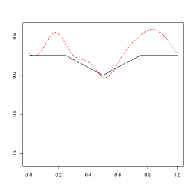
In this section we report the results of a Monte Carlo experiment to assess the performance of the proposed model selection procedure (3.18). In (1.1) we chose a -periodic function which, for is defined as
| (6.1) |
We simulate the model
where . Here is the semi-Markov process defined in (2.4) with a Gaussian sequence and used in (2.5) taken as .
We use the model selection procedure (3.18) with the weights (4.8) in which , , and . We define the empirical risk as
| (6.2) |
where the observation frequency and the expectations was taken as an average over replications, i.e.
We set the relative quadratic risk as
| (6.3) |
In our case . The table below gives the values for the sample risks (6.2) and (6.3) for different numbers of observations .
| n | ||
|---|---|---|
| 20 | 0.0398 | 0.211 |
| 100 | 0.0091 | 0.0483 |
| 200 | 0.0067 | 0.0355 |
| 1000 | 0.0022 | 0.0116 |
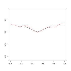
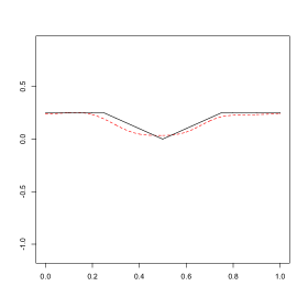
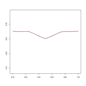
Figures 2–4 show the behavior of the regression function and its estimates by the model selection procedure (3.18) depending on the values of observation periods . The black full line is the regression function (6.1) and the red dotted line is the associated estimator.
Remark 6.1.
From numerical simulations of the procedure (3.18) with various observations numbers we may conclude that the quality of the proposed procedure is good for practical needs, i.e. for reasonable (non large) number of observations. We can also add that the quality of the estimation improves as the number of observations increases.
7 Proofs
7.1 Proof of Theorem 4.1
Using the cost function given in (3.15), we can rewrite the empirical squared error in (3.12) as follows
| (7.1) |
where
with and . Setting
| (7.2) |
we can rewrite (7.1) as
| (7.3) |
where and the function was defined in (3.10). Let be a fixed sequence in and be defined as in (3.17). Substituting and in Equation (7.3), we obtain
| (7.4) |
where , and . Note that, by (3.10),
The inequality
| (7.5) |
implies that, for any
Taking into account that , we get
where . Moreover, noting that in view of (3.10) , we can rewrite the previous bound as
| (7.6) |
To estimate the second term in the right side of this inequality we set
Thanks to (3.2) we estimate the term for any as
| (7.7) |
To estimate this function for a random vector , we set
So, through the Inequality (7.5), we get
| (7.8) |
It is clear that the last term here can be estimated as
| (7.9) |
where . Moreover, note that, for any ,
| (7.10) |
where . Taking into account now that, for any , the components , we can estimate this term as in (7.7), i.e.
Similarly to the previous reasoning we set
and we get
| (7.11) |
Using the same type of arguments as in (7.8), we can derive
| (7.12) |
From here and (7.10), we get
| (7.13) |
for any . Using this bound in (7.8) yields
Taking into account that , we obtain
Using this bound in (7.1) we obtain
Moreover, for we can rewrite this inequality as
Now, in view of the condition Proposition 5.3, we estimate the expectation of the term in (7.1) as
Now, taking into account that , we get
By using the upper bound for in Lemma A.1, we obtain that
Taking into account here that for and that and using the bounds (5.2) and (5.10) we obtain the inequality (4.2). Hence Theorem 4.1 .
7.2 Proof of Proposition 5.2
By Ito’s formula one gets
| (7.14) |
where . Taking into account that the processes and are independent and the time of jumps defined in (2.5) have a density, we have a.s. for any . Therefore, we can rewrite the differential (7.14) as
| (7.15) |
Therefore, using Lemma A.3 we obtain
where , is the density of the renewal measure and with the distribution of . Therefore,
| (7.16) |
where and . By the Ito formula we get
| (7.17) |
First, note that the process is a martingale and, using Lemma A.5, we get
The last integral can be represented as
where
By Lemma A.4 we get
where
We obtain directly that
and
From Lemma A.3 we obtain that
Therefore,
Taking into account that we can estimate the last integral as
From this and by the symmetry arguments we obtain that
| (7.18) |
Note now that
| (7.19) |
where
It should be noted that the continuous and the discrete parts of the processes (7.16) can be represented as
So, in view of Lemma 6.1 from [1],
| (7.20) |
with . Taking into account that and we can estimate the last integral as
Therefore,
| (7.21) |
To study the last term in (7.19) note that
Taking into account that for any
we obtain that
So, using the symmetry arguments, we find that
| (7.22) |
where
Note that
where
and
Now, similarly to (7.20) and taking into account that we get
So,
| (7.23) |
Moreover, taking into account that we get
So, in view of Lemma A.4
where
Noting now that
we obtain
Furthermore, the expectation of can be represented as
where the last term in this equality can be represented as
This implies
Therefore,
| (7.24) |
Finally we obtain that
| (7.25) |
As to the last term in (7.22) we can calculate directly
i.e.
From here we obtain that
| (7.26) |
where is given in (5.8). From this and (7.21) we find
| (7.27) |
7.3 Proof of Proposition 5.4
It is clear that the Inequality (5.11) holds true for . Let now . Setting and subtituting (3.8) in (3.14) yields,
| (7.28) |
where is defined in (7.2). Furthermore, putting , one can write the last term on the right hand side of (7.28) as
where the functions and are given in (5.1). Using Proposition 5.1, Proposition 5.3 and Lemma A.7 , we come to the following upper bound
Taking into account that and using the bounds (5.2) and (5.10) we obtain the inequality (5.11). Hence Proposition 5.4 holds true.
7.4 Proof of Theorem 4.3
7.5 Proof of Theorem 4.5
7.6 Proof of Proposition 4.6
First, we note that in view of (3.9) one can represent the quadratic risk for the empiric norm as
where . We put here for if The first term can be estimated by the bound (5.2) as
where . Therefore, taking into account that , we get
Note that
| (7.29) |
Furthermore, by the Inequality (7.5) for any we get
| (7.30) |
where . In view of Definition (4.8), we can represent this term as
where , and . Applying Lemma A.9 yields
Similarly, through Lemma A.8 we have
Hence,
where . Moreover, note that
Moreover, for any . From here and Lemma A.10 we get
Moreover, in view of Condition )
So,
To estimate the term we set
where the sequence is defined in (4.16). This leads to the inequality
Taking into account that , we get
where the coefficient is given in (4.8). This implies immediately that
| (7.31) |
Moreover, note that
So, applying (7.29) and (7.31), yields
| (7.32) |
Furthermore, Lemma A.6 yields that for any
So, in view of Condition ), we derive the desired inequality
Hence we obtain Proposition 4.6.
Acknowledgments. The last author is partially supported by the Russian Federal Professor program (Project No 1.472.2016/1.4, Ministry of Education and Science of the Russian Federation).
8 Appendix
A.1 Property of the penalty term
A.2 Properties of stochastic integrals (3.1)
In this section we give some results of stochastic calculus for the process given in (2.1), needed all along this paper. As the process is the combination of a Lévy process and a semi-Markov process, these results are not standard and need to be provided.
Lemma A.2.
Lemma A.3.
Lemma A.4.
Let and be bounded functions defined on Then, for any
where is the -field generated by the sequence , i.e., .
Lemma A.5.
Assume that Conditions – hold true. Then, for any measurable bounded non-random functions and , one has
A.3 Properties of the Fourier coefficients
Lemma A.6.
Let be an absolutely continuous function, with and be a simple function, of the form where are some constants. Then for any the function satisfies the following inequalities
Lemma A.7.
Lemma A.8.
For any , and , the coefficients of functions from the class satisfy, for any , the following inequality
| (A.3) |
Lemma A.9.
For any and , the coefficients of functions from the class satisfy the following inequality
| (A.4) |
Lemma A.10.
For any and the correction coefficients for the functions from the class satisfy the following inequality
| (A.5) |
References
- [1] V. S. Barbu, S. Beltaif and S. M. Pergamenchtchikov. Robust adaptive efficient estimation for semi-Markov nonparametric regression models. - Preprint, 25 March (2017), https://arxiv.org/pdf/1604.04516.pdf published in Statistical inference for stochastic processes.
- [2] O. E. Barndorff-Nielsen and N. Shephard. Non-Gaussian Ornstein-Uhlenbeck-based models and some of their uses in financial mathematics. J. Royal Stat. Soc., B 63, 167–241, 2001.
- [3] V. S. Barbu and N. Limnios. Semi-Markov Chains and Hidden Semi-Markov Models toward Applications - Their use in Reliability and DNA Analysis. Lecture Notes in Statistics, 191, Springer, New York, 2008.
- [4] N. Limnios and G. Oprisan. Semi-Markov Processes and Reliability. Birkhäuser, Boston, 2001.
- [5] C. M. Goldie. Implicit renewal theory and tails of solutions of random equations. The Annals of Applied Probability, 1 (1), 126–166, 1991.
- [6] I. A. Ibragimov and R. Z. Khasminskii. Statistical Estimation: Asymptotic Theory. Springer, Berlin–New York, 1981.
- [7] R. Cont, P. Tankov. Financial Modelling with Jump Processes. Chapman & Hall, 2004.
- [8] R. Höpfner and Yu. A. Kutoyants. Estimating discontinuous periodic signals in a time inhomogeneous diffusion. Statistical Inference for Stochastic Processes, 13 (3), 193–230, 2010.
- [9] R. Höpfner and Yu. A. Kutoyants. On LAN for parametrized continuous periodic signals in a time inhomogeneous diffusion. Statist. Decisions, 27 (4), 309–326, 2009.
- [10] J. Jacod, A. N. Shiryaev. Limit theorems for stochastic processes. Springer, Berlin, 2nd edition, 2002.
- [11] V. V. Konev and S. M. Pergamenshchikov. Sequential estimation of the parameters in a trigonometric regression model with the gaussian coloured noise. Statistical Inference for Stochastic Processes, 6, 215–235, 2003.
- [12] V. V. Konev and S. M. Pergamenshchikov. Nonparametric estimation in a semimartingale regression model. Part 1. Oracle Inequalities. Vestnik Tomskogo Universiteta, Mathematics and Mechanics, 3, 23–41, 2009.
- [13] V. V. Konev and S. M. Pergamenshchikov. Nonparametric estimation in a semimartingale regression model. Part 2. Robust asymptotic efficiency. Vestnik Tomskogo Universiteta, Mathematics and Mechanics, 4, 31–45, 2009.
- [14] V. V. Konev and S. M. Pergamenshchikov. General model selection estimation of a periodic regression with a Gaussian noise. Annals of the Institute of Statistical Mathematics, 62, 1083–1111, 2010.
- [15] V. V. Konev and S.M. Pergamenshchikov. Efficient robust nonparametric estimation in a semimartingale regression model. Ann. Inst. Henri Poincaré Probab. Stat., 48 (4), 1217–1244, 2012.
- [16] V.V. Konev and S.M. Pergamenshchikov. Robust model selection for a semimartingale continuous time regression from discrete data. Stochastic processes and their applications, 125, 294–326, 2015.
- [17] D. Lamberton and B. Lapeyre. Introduction to stochastic calculus applied to finance. Chapman & Hall, London, 1996.
- [18] T. Mikosch. Non-Life Insurance Mathematics. An Introduction with Stochastic Processes. Springer, 2004.
- [19] J. Jacod and A. N. Shiryaev. Limit theorems for stochastic processes. Vol.1, Springer, New York, 1987.
- [20] C. Mallows. Some comments on . Technometrics, 15, 661–675, 1973.
- [21] M. Nussbaum. Spline smoothing in regression models and asymptotic efficiency in . Ann. Statist., 13, 984–997, 1985.
- [22] M. S. Pinsker. Optimal filtration of square integrable signals in gaussian white noise. Problems of Transimission information, 17, 120–133, 1981.
- [23] R. Biard and B. Saussereau. Fractional Poisson processes: long-range dependence and applications in ruin theory. Applied Probability Trust, 2014.