SGDLibrary:
A MATLAB library for stochastic gradient descent algorithms

Abstract

We consider the problem of finding the minimizer of a function $f:\mathbb{R}^{d}\rightarrow\mathbb{R}$ of the finite-sum form $\min f(w)=1/n\sum_{i}^{n}f_{i}(w)$. This problem has been studied intensively in recent years in the field of machine learning (ML). One promising approach for large-scale data is to use a stochastic optimization algorithm to solve the problem. SGDLibrary is a readable, flexible and extensible pure-MATLAB library of a collection of stochastic optimization algorithms. The purpose of the library is to provide researchers and implementers a comprehensive evaluation environment for the use of these algorithms on various ML problems.

Published in Journal of Machine Learning Research (JMLR) entitled
“SGDLibrary: A MATLAB library for stochastic gradient optimization algorithms” [1]

1 Introduction

This work aims to facilitate research on stochastic optimization for large-scale data. We particularly address a regularized finite-sum minimization problem defined as

$$\min_{w\in\mathbb{R}^{d}}f(w):=\frac{1}{n}\sum_{i=1}^{n}f_{i}(w)=\frac{1}{n}\sum_{i=1}^{n}L(w,x_{i},y_{i})+\lambda R(w),$$ (1)

where $w\in\mathbb{R}^{d}$ represents the model parameter and $n$ denotes the number of samples $(x_{i},y_{i})$. $L(w,x_{i},y_{i})$ is the loss function and $R(w)$ is the regularizer with the regularization parameter $\lambda\geq 0$. Widely diverse machine learning (ML) models fall into this problem. Considering $L(w,x_{i},y_{i})=(w^{T}x_{i}-y_{i})^{2}$, $x_{i}\in\mathbb{R}^{d}$, $y_{i}\in\mathbb{R}$ and $R(w)=\|w\|_{2}^{2}$, this results in an $\ell_{2}$-norm regularized linear regression problem (a.k.a. ridge regression) for $n$ training samples $(x_{1},y_{1}),\cdots,({\color[rgb]{0,0,0}x_{n}},y_{n})$. In the case of binary classification with the desired class label $y_{i}\in\{+1,-1\}$ and $R(w)=\|w\|_{1}$, an $\ell_{1}$-norm regularized logistic regression (LR) problem is obtained as $f_{i}(w)=\log(1+\exp(-y_{i}w^{T}x_{i}))+\lambda\|w\|_{1}$, which encourages the sparsity of the solution of $w$. Other problems covered are matrix completion, support vector machines (SVM), and sparse principal components analysis, to name but a few.

Full gradient descent (a.k.a. steepest descent) with a step-size $\eta$ is the most straightforward approach for (1), which updates as $w_{k+1}\leftarrow w_{k}-{\color[rgb]{0,0,0}\eta}\nabla f(w_{k})$ at the $k$-th iteration. However, this is expensive when $n$ is extremely large. In fact, one needs a sum of $n$ calculations of the inner product $w^{T}x_{i}$ in the regression problems above, leading to $\mathcal{O}(nd)$ cost overall per iteration. For this issue, a popular and effective alternative is stochastic gradient descent (SGD), which updates as $w_{k+1}\leftarrow w_{k}-{\color[rgb]{0,0,0}\eta}\nabla f_{i}(w_{k})$ for the ${\color[rgb]{0,0,0}i}$-th sample uniformly at random [2, 3]. SGD assumes an unbiased estimator of the full gradient as $\mathbb{E}_{i}[\nabla f_{i}(w^{k})]=\nabla f(w^{k})$. As the update rule represents, the calculation cost is independent of $n$, resulting in $\mathcal{O}(d)$ per iteration. Furthermore, mini-batch SGD [3] calculates $1/|\mathcal{S}_{k}|\sum_{i\in\mathcal{S}_{k}}\nabla f_{i}(w_{k})$, where $\mathcal{S}_{k}$ is the set of samples of size $|\mathcal{S}_{k}|$. SGD needs a diminishing step-size algorithm to guarantee convergence, which causes a severe slow convergence rate [3]. To accelerate this rate, we have two active research directions in ML; Variance reduction (VR) techniques [4, 5, 6, 7, 8] that explicitly or implicitly exploit a full gradient estimation to reduce the variance of the noisy stochastic gradient, leading to superior convergence properties. Another promising direction is to modify deterministic second-order algorithms into stochastic settings, and solve the potential problem of first-order algorithms for ill-conditioned problems. A direct extension of quasi-Newton (QN) is known as online BFGS [9]. Its variants include a regularized version (RES) [10], a limited memory version (oLBFGS) [9, 11], a stochastic QN (SQN) [12], an incremental QN [13], and a non-convex version. Lastly, hybrid algorithms of the SQN with VR are proposed [14, 15]. Others include [16, 17].

The performance of stochastic optimization algorithms is strongly influenced not only by the distribution of data but also by the step-size algorithm [3]. Therefore, we often encounter results that are completely different from those in papers in every experiment. Consequently, an evaluation framework to test and compare the algorithms at hand is crucially important for fair and comprehensive experiments. One existing tool is Lightning [18], which is a Python library for large-scale ML problems. However, its supported algorithms are limited, and the solvers and the problems such as classifiers are mutually connected. Moreover, the implementations utilize Cython, which is a C-extension for Python, for efficiency. Subsequently, they decrease users’ readability of code, and also make users’ evaluations and extensions more complicated. SGDLibrary is a readable, flexible and extensible pure-MATLAB library of a collection of stochastic optimization algorithms. The library is also operable on GNU Octave. The purpose of the library is to provide researchers and implementers a collection of state-of-the-art stochastic optimization algorithms that solve a variety of large-scale optimization problems such as linear/non-linear regression problems and classification problems. This also allows researchers and implementers to easily extend or add solvers and problems for further evaluation. To the best of my knowledge, no report in the literature and no library describe a comprehensive experimental environment specialized for stochastic optimization algorithms. The code is available at https://github.com/hiroyuki-kasai/SGDLibrary.

2 Software architecture

The software architecture of SGDLibrary follows a typical module-based architecture, which separates problem descriptor and optimization solver. To use the library, the user selects one problem descriptor of interest and no less than one optimization solvers to be compared.

Problem descriptor: The problem descriptor, denoted as problem, specifies the problem of interest with respect to $w$, noted as w in the library. This is implemented by MATLAB classdef. The user does nothing other than calling a problem definition function, for instance, logistic_regression() for the $\ell_{2}$-norm regularized LR problem. Each problem definition includes the functions necessary for solvers; (i) (full) cost function $f(w)$, (ii) mini-batch stochastic derivative v=$1/|\mathcal{S}|\nabla f_{i\in\mathcal{S}}(w)$ for the set of samples $\mathcal{S}$. (iii) stochastic Hessian [17], and (iv) stochastic Hessian-vector product for a vector v. The built-in problems include, for example, $\ell_{2}$-norm regularized multidimensional linear regression, $\ell_{2}$-norm regularized linear SVM, $\ell_{2}$-norm regularized LR, $\ell_{2}$-norm regularized softmax classification (multinomial LR), $\ell_{1}$-norm multidimensional linear regression, and $\ell_{1}$-norm LR. The problem descriptor provides additional specific functions. For example, the LR problem includes the prediction and the classification accuracy calculation functions.

Optimization solver: The optimization solver implements the main routine of the stochastic optimization algorithm. Once a solver function is called with one selected problem descriptor problem as the first argument, it solves the optimization problem by calling some corresponding functions via problem such as the cost function and the stochastic gradient calculation function. Examples of the supported optimization solvers in the library are listed in categorized groups as; (i) SGD methods: Vanila SGD [2], SGD with classical momentum, SGD with classical momentum with Nesterov’s accelerated gradient [19], AdaGrad [16], RMSProp, AdaDelta, Adam, and AdaMax, (ii) Variance reduction (VR) methods: SVRG [4], SAG [5], SAGA [7], and SARAH [8], (iii) Second-order methods: SQN [17], oBFGS-Inf [9, 11], oBFGS-Lim (oLBFGS) [9, 11], Reg-oBFGS-Inf (RES) [10], and Damp-oBFGS-Inf, (iv) Second-order methods with VR: SVRG-LBFGS [15], SS-SVRG [15], and SVRG-SQN [14], and (v) Else: BB-SGD and SVRG-BB. The solver function also receives optional parameters as the second argument, which forms a struct, designated as options in the library. It contains elements such as the maximum number of epochs, the batch size, and the step-size algorithm with an initial step-size. Finally, the solver function returns to the caller the final solution w and rich statistical information, such as a record of the cost function values, the optimality gap, the processing time, and the number of gradient calculations.

Others: SGDLibrary accommodates a user-defined step-size algorithm. This accommodation is achieved by setting as options.stepsizefun=@my_stepsize_alg, which is delivered to solvers. Additionally, when the regularizer $R(w)$ in the minimization problem (1) is a non-smooth regularizer such as the $\ell_{1}$-norm regularizer $\|w\|_{1}$, the solver calls the proximal operator as problem.prox(w,stepsize), which is the wrapper function defined in each problem. The $\ell_{1}$-norm regularized LR problem, for example, calls the soft-threshold function as w = prox(w,stepsize)=soft_thresh(w,stepsize*lambda), where stepsize is the step-size $\eta$ and lambda is the regularization parameter $\lambda>0$ in (1).

3 Tour of the SGDLibrary

We embark on a tour of SGDLibrary exemplifying the $\ell_{2}$-norm regularized LR problem. The LR model generates $n$ pairs of $(x_{i},y_{i})$ for an unknown model parameter $w$, where $x_{i}$ is an input $d$-dimensional vector and $y_{i}\in\{-1,1\}$ is the binary class label, as $P(y_{i}|x_{i},w)=1/(1+\exp(-y_{i}w^{T}x_{i})).$ The problem seeks $w$ that fits the regularized LR model to the generated data $(x_{i},y_{i})$. This problem is cast as a minimization problem as $\min f(w):=1/n\sum_{i=1}^{n}\log[1+\exp(-y_{i}w^{T}x_{i})]+\lambda/2\|w\|^{2}.$ The code for this problem is in Listing 1.

⬇

1% generate synthetic 300 samples of dimension 3 for logistic regression

2d = logistic_regression_data_generator(300,3);

3% define logistic regression problem

4problem = logistic_regression(d.x_train,d.y_train,d.x_test,d.y_test);

5

6options.w_init = d.w_init; % set initial value

7options.step_init = 0.01; % set initial stepsize

8options.verbose = 1; % set verbose mode

9[w_sgd, info_sgd] = sgd(problem, options); % perform SGD solver

10[w_svrg, info_svrg] = svrg(problem, options); % perform SVRG solver

11[w_svrg, info_svrg] = sqn(problem, options); % perform SQN solver

12% display cost vs. number of gradient evaluations

13display_graph(’grad_calc_count’,’cost’,{’SGD’,’SVRG’},...

14 {w_sgd,w_svrg},{info_sgd,info_svrg});

Listing 1: Demonstration code for logistic regression problem.

First, we generate train/test datasets d using logistic_regression_data_generator(), where the input feature vector is with $n=300$ and $d=3$. $y_{i}\in\{-1,1\}$ is its class label. The LR problem is defined by calling logistic_regression(), which internally contains the functions for cost value, the gradient and the Hessian. This is stored in problem. Then, we execute solvers, i.e., SGD and SVRG, by calling solver functions, i.e., sgd() and svrg() with problem and options after setting some options into the options struct. They return the final solutions of {w_sgd,w_svrg} and the statistical information {info_sgd,info_svrg}. Finally, display_graph() visualizes the behavior of the cost function values in terms of the number of gradient evaluations. It is noteworthy that each algorithm requires a different number of evaluations of samples in each epoch. Therefore, it is common to use this value to evaluate the algorithms instead of the number of iterations. Illustrative results additionally including SQN and SVRG-LBFGS are presented in Figure 1, which are generated by display_graph(), and display_classification_result() specialized for classification problems. Thus, SGDLibrary provides rich visualization tools as well.

(a) Cost function value

(b) Optimality gap

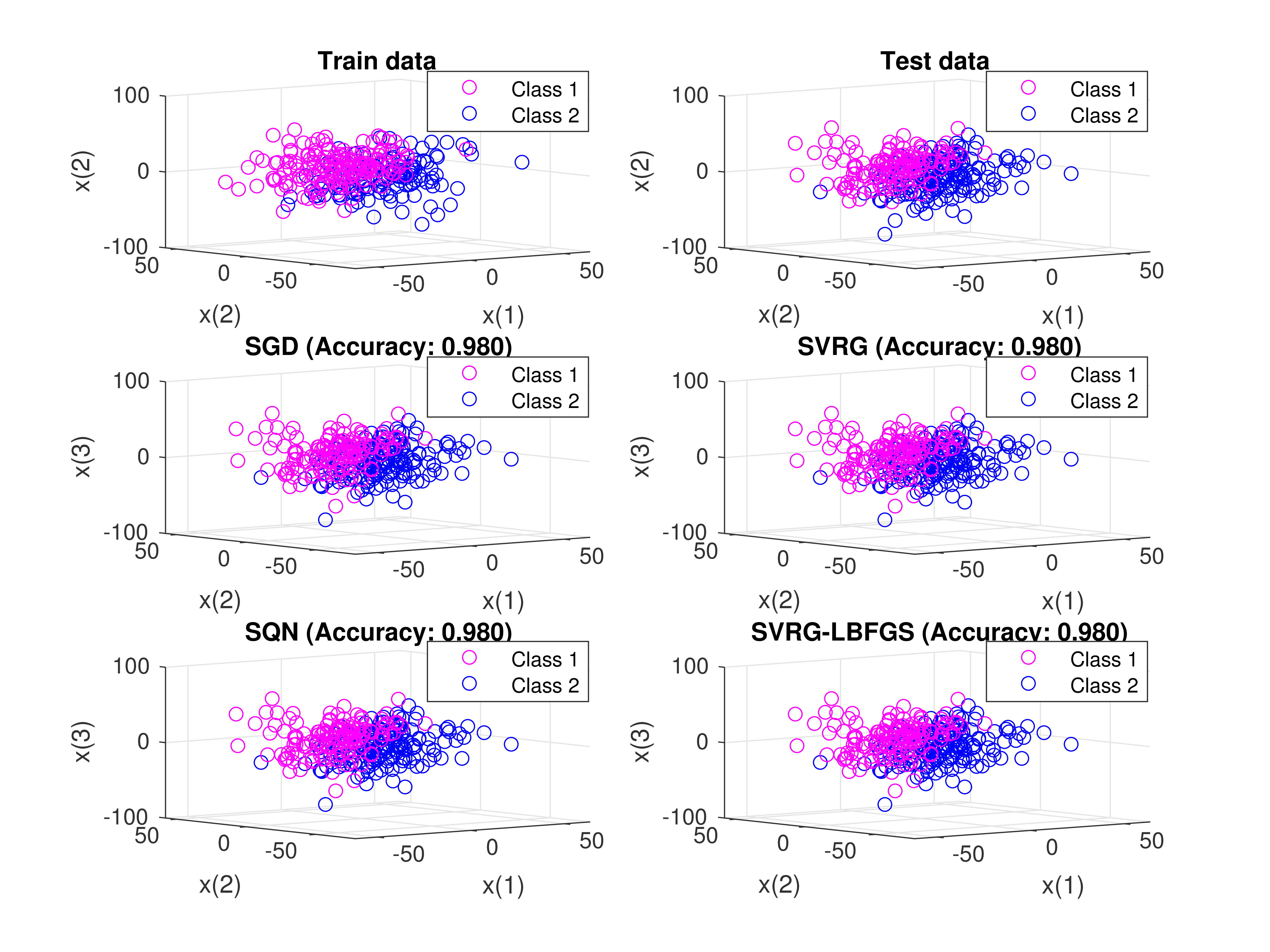
(c) Classification result

Figure 1: Results of $\ell_{2}$-norm regularized logistic regression problem.

Appendix A Supported stochastic optimization solvers

Table 1 summarizes the supported stochastic optimization algorithms and configurations.

Table 1: Supported stochastic optimization algorithms and configurations

algorithm name	solver	sub_mode	other options	Reference
SGD	sgd.m			[2]
SGD-CM	sgd_cm.m	CM
SGD-CM-NAG	sgd_cm.m	CM-NAG		[19]
AdaGrad	adagrad.m	AdaGrad		[16]
RMSProp	adagrad.m	RMSProp		[20]
AdaDelta	adagrad.m	AdaDelta		[21]
Adam	adam.m	Adam		[22]
AdaMax	adam.m	AdaMax		[22]
SVRG	svrg.m			[23]
SAG	sag.m	SAG		[24]
SAGA	sag.m	SAGA		[7]
SARAH	sarah.m			[8]
SARAH-Plus	sarah.m	Plus		[8]
SQN	slbfgs.m	SQN		[12]
oBFGS-Inf	obfgs.m	Inf-mem		[9]
oLBFGS-Lim	obfgs.m	Lim-mem		[9]
				[11]
Reg-oBFGS-Inf	obfgs.m	Inf-mem	delta $\neq 0$	[10]
Damp-oBFGS-Inf	obfgs.m	Inf-mem	delta $\neq 0$ &	[25]
			damped=true
IQN	iqn.m			[13]
SVRG-SQN	slbfgs.m	SVRG-SQN		[26]
SVRG-LBFGS	slbfgs.m	SVRG-LBFGS		[15]
SS-SVRG	subsamp			[15]
	_svrg.m
BB-SGD	bb_sgd.m			[27]
SVRG-BB	svrg_bb.m			[28]

Appendix B Directory and file structure

The tree structure below represents the directory and file structure of SGDLibrary. .1 /. .2 README.mdReadme file. .2 run$\_$me$\_$first.mFirst script to run. .2 demo.mDemonstration script to check library. .2 demo$\_$ext.mDemonstration script to check library. .2 sgdlibrary$\_$version.mVersion and release date information. .2 LICENSE.txtLicense file. .2 problem/Problem definitions. .2 sgd$\_$solver/Stochastic optimization sovlers. .2 sgd$\_$test/Test scripts to use this library. .2 plotter/Tools for plotting. .2 tool/Auxiliary tools. .2 gd$\_$solver/Gradient descent optimization solver files. .2 gd$\_$test/Test scripts for gradient descent solvers.

Appendix C How to use SGDLibrary

C.1 First to do

Run run_me_first for path configurations.

>> run_me_first;
##########################################################
###                                                    ###
###                Welcome to SGDLibrary               ###
###        (version:1.0.16, released:01-April-2017)    ###
###                                                    ###
##########################################################

Now, we are ready to use the library. Just execute demo for the simplest demonstration of this library. This is the case of $\ell_{2}$-norm regularized logistic regression problem.

>> demo;
SGD: Epoch = 000, cost = 3.3303581454622559e+01, optgap = Inf
SGD: Epoch = 001, cost = 1.1475439725295747e-01, optgap = Inf
............
SGD: Epoch = 099, cost = 7.9162101289075484e-02, optgap = Inf
SGD: Epoch = 100, cost = 7.8493133230913101e-02, optgap = Inf
Max epoch reached: max_epochr = 100
SVRG: Epoch = 000, cost = 3.3303581454622559e+01, optgap = Inf
SVRG: Epoch = 001, cost = 1.531453394302157711148737e-01, optgap = Inf
SVRG: Epoch = 002, cost = 9.330987606770735354189128e-02, optgap = Inf
............
SVRG: Epoch = 099, cost = 7.715265139028108787311311e-02, optgap = Inf
SVRG: Epoch = 100, cost = 7.715265135253832062822710e-02, optgap = Inf
Max epoch reached: max_epochr = 100

The cost function values every iteration of two algorithms are shown in the Matlab command window. Additionally, the convergence plots of the cost function values are shown as in Figure 2.

Figure 2: Result of $\ell_{2}$-norm regularized logistic regression problem.

C.2 Simplest usage example: 4 steps!

The code of demo.m is shown in Listing 2.

⬇

1% generate synthetic 300 samples of dimension 3 for logistic regression

2d = logistic_regression_data_generator(300,3);

3

4% define logistic regression problem

5problem = logistic_regression(d.x_train,d.y_train,d.x_test,d.y_test);

6

7options.w_init = d.w_init; % set initial value

8options.step_init = 0.01; % set initial stepsize

9opitons.verbose = 2; % set verbose mode

10[w_sgd, info_sgd] = sgd(problem, options); % perform SGD solver

11[w_svrg, info_svrg] = svrg(problem, options); % perform SVRG solver

12

13% display cost vs. number of gradient evaluations

14display_graph(’grad_calc_count’,’cost’,{’SGD’,’SVRG’},...

15 {w_sgd,w_svrg},{info_sgd,info_svrg});

Listing 2: Demonstration code for the logistic regression problem

Let us take a closer look at the code above bit by bit. The procedure has only 4 steps!

Step 1: Generate data

First, we generate datasets including train set and test set using a data generator function logistic_regression_data_generator(). The output includes train & test set and an initial value of the solution w.

⬇

1% generate synthetic 300 samples of dimension 3 for logistic regression

2d = logistic_regression_data_generator(300,3);

Listing 3: Code for data generation.

Step 2: Define problem

The problem to be solved should be defined properly from the supported problems. logistic_regression() provides the comprehensive functions for a logistic regression problem. This returns the cost value by cost(w), the gradient by grad(w) and the hessian by hess(w) when given w. These are essential for any gradient descent algorithms.

⬇

4% define logistic regression problem

5problem = logistic_regression(d.x_train,d.y_train,d.x_test,d.y_test);

Listing 4: Code for problem definition.

Step 3: Perform solver

Now, you can perform optimization solvers, i.e., SGD and SVRG, calling solver functions, i.e., sgd() function and svrg() function, after setting some optimization options as the options struct.

⬇

7options.w_init = d.w_init; % set initial value

8options.step_init = 0.01; % set initial stepsize

9opitons.verbose = 2; % set verbose mode

10[w_sgd, info_sgd] = sgd(problem, options); % perform SGD solver

11[w_svrg, info_svrg] = svrg(problem, options); % perform SVRG solver

Listing 5: Code for optimization solver execution.

They return the final solutions of w and the statistics information that include the histories of the epoch numbers, the cost function values, norms of gradient, the number of gradient evaluations and so on.

Step 4: Show result

Finally, display_graph() provides output results of decreasing behavior of the cost values in terms of the number of gradient evaluations. Note that each algorithm needs different number of evaluations of samples in each epoch. Therefore, it is common to use this number to evaluate stochastic optimization algorithms instead of the number of iterations.

⬇

13% display cost vs. number of gradient evaluations

14display_graph(’grad_calc_count’,’cost’,{’SGD’,’SVRG’},...

15 {w_sgd,w_svrg},{info_sgd,info_svrg});

Listing 6: Code for showing results.

Appendix D Problem definition

This specifies the problem of interest with respect to w, noted as w in the library. It is noteworthy that the problem is defined as the class-based structure by exploiting MATLAB classdef.

The user does nothing other than calling a problem definition function.

The build-in problems in the library include

• $\ell_{2}$-norm regularized multidimensional linear regression

• $\ell_{2}$-norm regularized linear support vector machines (SVM)

• $\ell_{2}$-norm regularized logistic regression (LR)

• $\ell_{2}$-norm regularized softmax classification (multinomial LR)

• $\ell_{1}$-norm regularized multidimensional linear regression

• $\ell_{1}$-norm regularized logistic regression (LR)

Each problem definition contains the functions necessary for solvers;

• cost(w): calculate full cost function $f(w)$,

• grad(w,indices) : calculate mini-batch stochastic derivative $\verb+v+=1/|\mathcal{S}|\nabla f_{i\in\mathcal{S}}(w)$ for the set of samples $\mathcal{S}$, which is noted as indices.

• hess(w,indices): calculate stochastic Hessian for indices.

• hess_vec(w,v,indices): calculate stochastic Hessian-vector product for v and indices.

We illustrate the code of the definition of $\ell_{2}$-norm regularized linear regression function as an example. Listing 7 shows its entire code of linear_regression() function.

⬇

1classdef linear_regression

2 properties

3 name;

4 dim;

5 samples;

6 lambda;

7 hessain_w_independent;

8 d;

9 n_train;

10 n_test;

11 x_train;

12 y_train;

13 x_test;

14 y_test;

15 x_norm;

16 x;

17 end

18

19 methods

20 % define constructor

21 function obj=linear_regression(x_train, y_train, x_test, y_test, varargin)

22 obj.x_train = x_train;

23 obj.y_train = y_train;

24 obj.x_test = x_test;

25 obj.y_test = y_test;

26 if nargin < 5; obj.lambda = 0.1;

27 else; obj.lambda = varargin{1}; end

28

29 obj.d = size(x_train, 1);

30 obj.n_train = length(y_train);

31 obj.n_test = length(y_test);

32 obj.name = ’linear_regression’;

33 obj.dim = obj.d;

34 obj.samples = obj.n_train;

35 obj.hessain_w_independent = true;

36 obj.x_norm = sum(x_train.^2,1);

37 obj.x = x_train;

38 end

39

40 % define cost function

41 function f = cost(obj, w)

42 f = sum((w’*obj.x_train-obj.y_train).^2)/(2 * obj.n_train) ...

43 + obj.lambda/2*w’*w;

44 end

45

46 % define stochastic gradient

47 function g = grad(obj, w, indices)

48 residual = w’*obj.x_train(:,indices) - obj.y_train(indices);

49 g = obj.x_train(:,indices) * residual’/length(indices) ...

50 + obj.lambda*w;

51 end

52

53 % define full gradient

54 function g = full_grad(obj, w)

55 g = obj.grad(w, 1:obj.n_train);

56 end

57

58 % define stochastic hessian

59 function h = hess(obj, w, indices)

60 h = 1/length(indices) * obj.x_train(:,indices) ...

61 * (obj.x_train(:,indices)’) + obj.lambda * eye(obj.d);

62 end

63

64 % define full hessian

65 function h = full_hess(obj, w)

66 h = hess(w, 1:obj.n_train);

67 end

68

69 % define stochastic hessian-vector

70 function hv = hess_vec(obj, w, v, indices)

71 hv = 1/length(indices) * obj.x_train(:,indices) ...

72 * ((obj.x_train(:,indices)’*v)) + obj.lambda*v;

73 end

74

75 % define prediction function

76 function p = prediction(obj, w)

77 p = w’ * obj.x_test;

78 end

79

80 % define mse calculation function

81 function e = mse(obj, y_pred)

82 e = sum((y_pred-obj.y_test).^2)/(2 * obj.n_test);

83 end

84 end

85end

Listing 7: Demonstration code for linear regression problem.

We explain line-by-line of Listing 7 below;

Listing 8 defines the properties (i.e., class variables) properties of the class.

⬇

2 properties

3 name;

4 dim;

5 samples;

6 lambda;

7 hessain_w_independent;

8 d;

9 n_train;

10 n_test;

11 x_train;

12 y_train;

13 x_test;

14 y_test;

15 x_norm;

16 x;

17 end

Listing 8: Properties for linear regression problem class.

Listing 9 defines the constructor linear_regression() of the class.

⬇

20 % define constructor

21 function obj=linear_regression(x_train, y_train, x_test, y_test, varargin)

22 obj.x_train = x_train;

23 obj.y_train = y_train;

24 obj.x_test = x_test;

25 obj.y_test = y_test;

26 if nargin < 5; obj.lambda = 0.1;

27 else; obj.lambda = varargin{1}; end

28

29 obj.d = size(x_train, 1);

30 obj.n_train = length(y_train);

31 obj.n_test = length(y_test);

32 obj.name = ’linear_regression’;

33 obj.dim = obj.d;

34 obj.samples = obj.n_train;

35 obj.hessain_w_independent = true;

36 obj.x_norm = sum(x_train.^2,1);

37 obj.x = x_train;

38 end

Listing 9: Constructor for linear regression problem class.

Listing 10 defines the cost calculation function cost() with respect to w.

⬇

40 % define cost function

41 function f = cost(obj, w)

42 f = sum((w’*obj.x_train-obj.y_train).^2)/(2 * obj.n_train) ...

43 + obj.lambda/2*w’*w;

44 end

Listing 10: Cost function code for linear regression problem class.

Listing 11 defines the stochastic gradient calculation function grad() with respect to w for indices. full_grad() calculates the full gradient estimation.

⬇

53 % define cost function

54 function f = cost(obj, w)

55 f = sum((w’*obj.x_train-obj.y_train).^2)/(2 * obj.n_train) ...

56 + obj.lambda/2*w’*w;

57 end

58

59 % define stochastic gradient

60 function g = grad(obj, w, indices)

61 residual = w’*obj.x_train(:,indices) - obj.y_train(indices);

62 g = obj.x_train(:,indices) * residual’/length(indices) ...

63 + obj.lambda*w;

64 end

Listing 11: Gradient calculation function code for linear regression problem class.

Listing 12 defines the stochastic Hessian calculation function hess() with respect to w for indices. full_hess() calculates the full Hessian estimation.

⬇

64 % define stochastic hessian

65 function h = hess(obj, w, indices)

66 h = 1/length(indices) * obj.x_train(:,indices) ...

67 * (obj.x_train(:,indices)’) + obj.lambda * eye(obj.d);

68 end

69

70 % define full hessian

71 function h = full_hess(obj, w)

72 h = hess(w, 1:obj.n_train);

73 end

Listing 12: Hessian calculation function code for linear regression problem class.

Listing 13 defines the stochastic Hessian-vector product calculation function hess_vec() with respect to w and a vector v for indices.

⬇

70 % define stochastic hessian-vector

71 function hv = hess_vec(obj, w, v, indices)

72 hv = 1/length(indices) * obj.x_train(:,indices) ...

73 * ((obj.x_train(:,indices)’*v)) + obj.lambda*v;

74 end

Listing 13: Hessian-vector product calculation function code for linear regression problem class.

The problem descriptor also provides some specific functions that are necessary for a particular problem. For example, the linear regression problem predicts the class for test data based on the model parameter that is trained by a stochastic optimization algorithm. Then, the final classification are calculated. Therefore, the regression problem equips the prediction and the mean squares error (MSE) calculation functions.

• prediction(w)

• mse(y_pred)

Listing 14 shows the prediction function prediction from the final solution w, and the MSE calculation function mse.

⬇

75 % define prediction function

76 function p = prediction(obj, w)

77 p = w’ * obj.x_test;

78 end

79

80 % define mse calculation function

81 function e = mse(obj, y_pred)

82 e = sum((y_pred-obj.y_test).^2)/(2 * obj.n_test);

83 end

Listing 14: Prediction and MSE calculation code for linear regression problem class.

Meanwhile, in case of the logistic regression problem, the final classification are calculated. Therefore, the regression problem equips the prediction and the prediction accuracy calculation functions.

• prediction(w)

• accuracy(y_pred)

Listing 15 illustrates the binary-class prediction function prediction with the final solution w, and prediction accuracy calculation function accuracy with the predicted classes.

⬇

1 % define prediction function

2 Problem.prediction = @prediction;

3 function p = prediction(w)

4 p = sigmoid(w’ * x_test);

5 class1_idx = p>0.5;

6 class2_idx = p<=0.5;

7 p(class1_idx) = 1;

8 p(class2_idx) = -1;

9 end

10

11 % define prediction accuracy calculation function

12 Problem.accuracy = @accuracy;

13 function a = accuracy(y_pred)

14 a = sum(y_pred == y_test)/n_test;

15 end

Listing 15: Prediction and prediction accuracy calculation code for logistric regression problem.

The last example is the softmax regression problem case. This case also contains the prediction function prediction and the prediction accuracy calculation function accuracy as shown in Listing 16.

⬇

1 % define prediction function

2 Problem.prediction = @prediction;

3 function max_class = prediction(w)

4 w_mat = reshape(w, [d n_classes]);

5 p = w_mat’ * x_test;

6 [~, max_class] = max(p, [], 1);

7 end

8

9 % define prediction accuracy calculation function

10 Problem.accuracy = @accuracy;

11 function a = accuracy(class_pred)

12 [~, class_test] = max(y_test, [], 1);

13 a = sum(class_pred == class_test) / n_test;

14 end

Listing 16: Prediction and prediction accuracy calculation code for softmax regression problem.

Appendix E Solver definition

This implements the main routine of the stochastic optimization solver. The optimization solver solves an optimization problem by calling the corresponding functions via the problem definition, such as cost(w), grad(w,indices), and possibly hess(w,indices). The final optimal solution w and the statistic information are returned. The latter is stored as the info struct. See also Appendix H.

This section illustrates the definition of the SGD function sgd() as an example. The entire code of sgd() is shown in Listing 17.

⬇

1function [w,infos]=sgd(problem, in_options)

2 n=problem.samples(); % number of samples

3

4 % set options

5 local_options=[];

6 options=mergeOptions(get_default_options(problem.dim()),local_options);

7 options=mergeOptions(options,in_options);

8

9 % initialize

10 iter=0; epoch=0; grad_calc_count=0;

11 w=options.w_init;

12 num_of_bachces=floor(n/options.batch_size);

13

14 % store first statistics infos

15 infos=store_infos(problem,w,options,[],epoch,grad_calc_count,0);

16

17 % outer loop

18 s_time = tic();

19 while(optgap>options.tol_optgap) && (epoch<options.max_epoch)

20 perm_idx = randperm(n); % permute samples

21

22 % inner loop

23 for j = 1 : num_of_bachces

24 step=options.stepsizefun(iter,options); % step-size

25

26 s_index=(j-1)*options.batch_size+1;

27 indice_j=perm_idx(s_index:s_index+options.batch_size-1);

28 grad=problem.grad(w, indice_j); % calculate gradient

29

30 w=w-step*grad; % update w

31

32 if isfield(problem,’prox’) % proximal operator

33 w=problem.prox(w, step);

34 end

35

36 iter=iter+1;

37 end

38

39 grad_calc_count=grad_calc_count+num_of_bachces*options.batch_size;

40 epoch=epoch+1;

41

42 % store statistics infos

43 infos=store_infos(problem,w,options,infos,epoch,...

44 grad_calc_count,toc(s_time));

45 end

46end

Listing 17: Demonstration code for SGD solver.

We explain line-by-line of Listing 17 below.

We first set option parameters as a options struct. The solver merges the local default options local_options, the default options get_default_options() that are commonly used in all solvers, and the input options in_options. This is shown in Listing 18.

⬇

4 % set options

5 local_options=[];

6 options=mergeOptions(get_default_options(problem.dim()),local_options);

7 options=mergeOptions(options,in_options);

Listing 18: Optional parameter configuration code for SGD solver.

Next, the initial statistics data are collected by store_infos function as shown in Listing 19 before entering the main optimization routine. The statistics data are also collected at the end of every epoch, i.e., outer iteration, as Listing 20. See also Appendix H.

⬇

113 % store first statistics infos

114 infos=store_infos(problem,w,options,[],epoch,grad_calc_count,0);

Listing 19: Initial statistics data collection code for SGD solver.

⬇

141 % store statistics infos

142 infos=store_infos(problem,w,options,infos,epoch,...

143 grad_calc_count,toc(s_time));

Listing 20: Statistics data collection code for SGD solver.

The code in Listing 21 shows the calculation of the stepsize. If the user does not specify his/her user-defined stepsize algorithm, the solver calls a default stepsize algorithm function with options parameter. This parameter contains the stepsize algorithm type, the initial stepsize and so on. Otherwise, the user-defined stepsize algorithm is called. See also Appendix G.

⬇

24 step=options.stepsizefun(iter,options); % step-size

Listing 21: Stepsize calculation code for SGD solver.

Listing 22 illustrates the code for the stochastic gradient calculation, where indice_j is calculated from the number of the inner iteration, j, and the batch size options.batch_size.

⬇

26 s_index=(j-1)*options.batch_size+1;

27 indice_j=perm_idx(s_index:s_index+options.batch_size-1);

28 grad=problem.grad(w, indice_j); % calculate gradient

Listing 22: Stochastic gradient calculation code for SGD solver.

Finally, the model parameter w is updated using the calculated stepsize step and the stochastic gradient grad as Listing 23.

⬇

30 w=w-step*grad; % update w

Listing 23: Mode parameter update code for SGD solver.

Appendix F Default stepsize algorithms

SGDLibrary supports four stepsize algorithms. This can be switched by the setting option struct such as options.step_alg=’decay-2’. After $\eta_{0}(=\verb+options.step_init+)$ and $\lambda(=\verb+options.lambda+)$ are properly configured, we can use one of the following algorithms according to the total inner iteration number $k$ as;

• fix: This case uses below;

  $$\eta = \eta_{0}.$$

• decay : This case uses below;

  $$\eta = \frac{\eta_{0}}{1+\eta_{0}\lambda k}.$$

• decay-2: This case uses below;

  $$\eta = \frac{\eta_{0}}{1+k}.$$

• decay-3: This case uses below;

  $$\eta = \frac{\eta_{0}}{\lambda+k}.$$

SGDLibrary also accommodates a user-defined stepsize algorithm. See the next section.

Appendix G User-defined stepsize algorithm

SGDLibrary allows the user to define a new user-defined stepsize algorithm. This is done by setting as options.stepsizefun = @my_stepsize_alg, which is delivered to solvers via their input arguments. The illustrative example code is shown in Listing 24.

⬇

1function stepsize_alg_demo()

2 % generate synthetic 1000 samples of dimension 10

3 d = logistic_regression_data_generator(1000,10);

4

5 % define logistic regression problem

6 problem = logistic_regression(d.x_train, d.y_train, d.x_test, d.y_test);

7

8 options.w_init = d.w_init; % set initial value

9 options.step_init = 0.01; % set initial stepsize

10 options.step_alg = ’decay’; % set decay stepsize algorithm

11 [w_sgd,info_sgd] = sgd(problem, options); % perform SGD solver

12 options.stepsizefun = @my_stepalg; % set my_stepalg stepsize algorithm

13 [w_sgd_my,info_sgd_my] = sgd(problem, options);% perform SGD solver

14

15 % display cost/optimality gap vs number of gradient evaluations

16 display_graph(’grad_calc_count’,’cost’,{’SGD(decay)’,’SGD(My algorithm)’},{w_sgd, w_sgd_my},{info_sgd,info_sgd_my});

17end

18

19% define user-defined stepsize algorithm

20function step = my_stepalg(iter,options)

21 step = options.step_init/(10+iter*0.5);

22end

Listing 24: Demonstration code for user-define stepsize algorithm.

Listing 25 defines an example of the user-defined stepsize algorithm named as my_stepalg.

⬇

19% define user-defined stepsize algorithm

20function step = my_stepalg(iter,options)

21 step = options.step_init/(10+iter*0.5);

22end

Listing 25: Definition code of user-define stepsize algorithm.

Then, the new algorithm function my_stepalg is set to the algorithm via options value for each solver as shown in Listing 26.

⬇

12 options.stepsizefun = @my_stepalg; % set my_stepalg stepsize algorithm

Listing 26: Setting code of user-define stepsize algorithm.

Appendix H Collect statistics information

The solver automatically collects statistics information every epoch, i.e., outer iteration, via store_infos() function. The collected data are stored in infos struct, and it is returned to the caller function to visualize the results. The information contain below.

• iter: number of iterations

• time: elapsed time

• grad_calc_count: count of gradient calculations

• optgap: optimality gap

• cost: cost function value

• gnorm: norm of full gradient

Additionally, when a regularizer exists, its value is collected. This provides informative information, for example, the sparsity when $R(w)=\|w\|_{1}$. Furthermore, the user can collect the history of solution w in every epoch.

The code of store_infos() is illustrated in Listing 27.

⬇

1function [infos,f_val,optgap] = store_infos(problem,w,options,infos,...

2 epoch,grad_calc_count,elapsed_time)

3 % calculation of cost function value

4 f_val = problem.cost(w);

5 % calculation of norm of full gradient

6 gnorm = norm(problem.full_grad(w));

7 % calculation of optimality gap

8 optgap = f_val - options.f_opt;

9

10 % number of iterations

11 infos.iter = [infos.iter epoch];

12 % elapsed time

13 infos.time = [infos.time elapsed_time];

14 % count of gradient calculations

15 infos.grad_calc_count = [infos.grad_calc_count grad_calc_count];

16 % optimality gap

17 infos.optgap = [infos.optgap optgap];

18 % cost function value

19 infos.cost = [infos.cost f_val];

20 % norm of full gradient

21 infos.gnorm = [infos.gnorm gnorm];

22 % value of regularizer

23 if isfield(problem, ’reg’)

24 reg = problem.reg(w);

25 infos.reg = [infos.reg reg];

26 end

27 % solution w

28 if options.store_w

29 infos.w = [infos.w w];

30 end

31end

Listing 27: Statistic information collection code.

Appendix I Visualizations

SGDLibrary provides various visualization tools, which include

• display_graph(): display various graphs such as cost function values vs. the number of gradient evaluations, and the optimality gap vs. the number of gradient evaluations.

• display_regression_result(): show regression results for regression problems.

• display_classification_result(): show classification results specialized for classification problems.

• draw_convergence_animation(): draw convergence behavior animation of solutions.

This section provides illustrative explanations in case of $\ell_{2}$-norm regularized logistic regression problem. The entire code is shown in Listing 28.

⬇

1% generate synthetic 300 samples of dimension 2 for logistic regression

2d=logistic_regression_data_generator(300,2);

3

4% define problem definitions

5problem=logistic_regression(d.x_train,d.y_train,d.x_test,d.y_test);

6

7w_opt=problem.calc_solution(problem,1000); % calculate optimal w

8options.f_opt=problem.cost(w_opt); % calculate optimal f

9options.store_w=true; % store w for convergence animation

10

11options.w_init=d.w_init; % set initial value

12options.step_init=0.01; % set initial stepsize

13[w_sgd,info_sgd]= gd(problem,options); % perform SGD solver

14[w_svrg,info_svrg]=svrg(problem,options); % perform SVRG solver

15

16% display cost/optimality gap vs number of gradient evaluations

17display_graph(’grad_calc_count’,’cost’,{’SGD’,’SVRG’},...

18 {w_sgd,w_svrg},{info_sgd,info_svrg});

19display_graph(’grad_calc_count’,’optimality_gap’,{’SGD’,’SVRG’},...

20 {w_sgd,w_svrg},{info_sgd,info_svrg});

21

22% display classification results

23y_pred_sgd=problem.prediction(w_sgd); % predict for SGD

24accuracy_sgd=problem.accuracy(y_pred_sgd); % calculate accuracy for SGD

25fprintf(’Classificaiton accuracy:%s:%.4f\n’,’SGD’,accuracy_sgd);

26y_pred_sgd(y_pred_sgd==-1)=2; % convert from {1,-1} to {1,2}

27y_pred_sgd(y_pred_sgd==1)=1;

28y_pred_svrg = problem.prediction(w_svrg); % predict for SVRG

29accuracy_svrg=problem.accuracy(y_pred_svrg);% calculate accuracy for SVRG

30fprintf(’Classificaiton accuracy:%s:%.4f\n’,’SVRG’,accuracy_svrg);

31y_pred_svrg(y_pred_svrg==-1) = 2; % convert from {1,-1} to {1,2}

32y_pred_svrg(y_pred_svrg==1) = 1;

33d.y_train(d.y_train==-1)=2; d.y_train(d.y_train==1)=1;

34d.y_test(d.y_test==-1)=2; d.y_test(d.y_test==1)=1;

35display_classification_result(problem, {’SGD’,’SVRG’},{w_sgd,w_svrg}, ...

36 {y_pred_sgd,y_pred_svrg},{accuracy_sgd,accuracy_svrg}, ...

37 d.x_train,d.y_train,d.x_test,d.y_test);

38

39% display convergence animation

40draw_convergence_animation(problem,{’SGD’,’SVRG’},...

41 {info_sgd.w,info_svrg.w},100,0.1);

Listing 28: Demonstration code for result visualization.

First, for the calculation of optimality gap, the user needs the optimal solution w_opt beforehand. This is obtained by calling problem.calc_solution() function of the problem definition function. This case uses the L-BFGS solver inside it to obtain the optimal solution under maximum iteration $1000$ with a very precise tolerant stopping condition. Then, the optimal cost function value f_opt is calculated from w_opt. Listing 29 shows the code.

⬇

7w_opt=problem.calc_solution(problem,1000); % calculate optimal w

8options.f_opt=problem.cost(w_opt); % calculate optimal f

Listing 29: Optimal solution and cost function value calculation code.

Then, you obtain the result of the optimality gap by display_graph() as Listing 30. The first argument and the second argument correspond to the values of $x$-axis and $y$-axis, respectively, in the graph. We can change these values according to the statistics data explained in Appendix H. The third argument represents the list of the algorithm names that are shown in the legend of the graph. The forth parameter indicates the list of the info structs to be shown.

⬇

16% display cost/optimality gap vs number of gradient evaluations

17display_graph(’grad_calc_count’,’cost’,{’SGD’,’SVRG’},...

18 {w_sgd,w_svrg},{info_sgd,info_svrg});

19display_graph(’grad_calc_count’,’optimality_gap’,{’SGD’,’SVRG’},...

20 {w_sgd,w_svrg},{info_sgd,info_svrg});

Listing 30: Display graph code.

Additionally, in case of $\ell_{2}$-norm regularized logistic regression problems, the results of classification accuracy are calculated using the corresponding prediction function probrem.prediction() and the accuracy calculating function probrem.accuracy(). Then, the classification accuracies are illustrated by display_classification_result() function. The code is shown as Listing 31.

⬇

22% display classification results

23y_pred_sgd=problem.prediction(w_sgd); % predict for SGD

24accuracy_sgd=problem.accuracy(y_pred_sgd); % calculate accuracy for SGD

25fprintf(’Classificaiton accuracy:%s:%.4f\n’,’SGD’,accuracy_sgd);

26y_pred_sgd(y_pred_sgd==-1)=2; % convert from {1,-1} to {1,2}

27y_pred_sgd(y_pred_sgd==1)=1;

28y_pred_svrg = problem.prediction(w_svrg); % predict for SVRG

29accuracy_svrg=problem.accuracy(y_pred_svrg);% calculate accuracy for SVRG

30fprintf(’Classificaiton accuracy:%s:%.4f\n’,’SVRG’,accuracy_svrg);

31y_pred_svrg(y_pred_svrg==-1) = 2; % convert from {1,-1} to {1,2}

32y_pred_svrg(y_pred_svrg==1) = 1;

33d.y_train(d.y_train==-1)=2; d.y_train(d.y_train==1)=1;

34d.y_test(d.y_test==-1)=2; d.y_test(d.y_test==1)=1;

35display_classification_result(problem, {’SGD’,’SVRG’},{w_sgd,w_svrg}, ...

36 {y_pred_sgd,y_pred_svrg},{accuracy_sgd,accuracy_svrg}, ...

37 d.x_train,d.y_train,d.x_test,d.y_test);

Listing 31: Display classification results code.

Figure 3: Logistic regression problem.

Finally, you can also show a demonstration of convergence animation. You need specify additional options before executing solvers as Listing 32.

⬇

9options.store_w=true; % store w for convergence animation

Listing 32: Store history of solutions.

Now, the animation of the convergence behavior is shown. The code is shown in Listing 33. It should be noted that draw_convergence_animation() is executable when only the dimension $d$ of the parameters is $2$. The last parameter for the function, i.e., $0.1$ in this example, indicates the speed of the animation.

⬇

39% display convergence animation

40draw_convergence_animation(problem,{’SGD’,’SVRG’},...

41 {info_sgd.w,info_svrg.w},100,0.1);

Listing 33: Draw convergence animation.

Figure 4: convergence animation.

Appendix J More results

We show more results for $\ell_{2}$-norm regularized linear regression problem, $\ell_{2}$-norm softmax classifier problem, and $\ell_{2}$-norm regularized linear SVM problem in Figures 5 to 7, respectively.

Figure 5: Linear regression problem.

Figure 6: Softmax classifier problem.

Figure 7: Linear SVM problem.

References

- [1] H. Kasai. SGDLibrary: A MATLAB library for stochastic gradient optimization algorithms. J. Mach. Learn. Res., 18(215):1–5, 2018.
- [2] H. Robbins and S. Monro. A stochastic approximation method. Ann. Math. Statistics, 22(3):400–407, 1951.
- [3] L. Bottou. Online algorithm and stochastic approximations. In David Saad, editor, On-Line Learning in Neural Networks. Cambridge University Press, 1998.
- [4] R. Johnson and T. Zhang. Accelerating stochastic gradient descent using predictive variance reduction. In NIPS, 2013.
- [5] N. L. Roux, M. Schmidt, and F. R. Bach. A stochastic gradient method with an exponential convergence rate for finite training sets. In NIPS, 2012.
- [6] S. Shalev-Shwartz and T. Zhang. Stochastic dual coordinate ascent methods for regularized loss minimization. J. Mach. Learn. Res., 14:567–599, 2013.
- [7] A. Defazio, F. Bach, and S. Lacoste-Julien. SAGA: A fast incremental gradient method with support for non-strongly convex composite objectives. In NIPS, 2014.
- [8] L. M. Nguyen, J. Liu, K. Scheinberg, and M. Takac. SARAH: A novel method for machine learning problems using stochastic recursive gradient. In ICML, 2017.
- [9] N. N. Schraudolph, J. Yu, and S. Gunter. A stochastic quasi-Newton method for online convex optimization. In AISTATS, 2007.
- [10] A. Mokhtari and A. Ribeiro. RES: Regularized stochastic BFGS algorithm. IEEE Trans. on Signal Process., 62(23):6089–6104, 2014.
- [11] A. Mokhtari and A. Ribeiro. Global convergence of online limited memory BFGS. J. Mach. Learn. Res., 16:3151–3181, 2015.
- [12] R. H. Byrd, S. L. Hansen, J. Nocedal, and Y. Singer. A stochastic quasi-Newton method for large-scale optimization. SIAM J. Optim., 26(2), 2016.
- [13] A. Mokhtari, M. Eizen, and A. Ribeiro. An incremental quasi-Newton method with a local superlinear convergence rate. In ICASSP, 2017.
- [14] P. Moritz, R. Nishihara, and M. I. Jordan. A linearly-convergent stochastic L-BFGS algorithm. In AISTATS, 2016.
- [15] R. Kolte, M. Erdogdu, and A. Ozgur. Accelerating SVRG via second-order information. In OPT2015, 2015.
- [16] J. Duchi, E. Hazan, and Y. Singer. Adaptive subgradient methods for online learning and stochastic optimization. J. Mach. Learn. Res., 12:2121–2159, 2011.
- [17] A. Bordes, L. Bottou, and P. Callinari. SGD-QN: Careful quasi-Newton stochastic gradient descent. J. Mach. Learn. Res., 10:1737–1754, 2009.
- [18] M. Blondel and F. Pedregosa. Lightning: large-scale linear classification, regression and ranking in Python, 2016.
- [19] I. Sutskever, J. Martens, G. Dahl, and G. Hinton. On the importance of initialization and momentum in deep learning. In ICML, 2013.
- [20] G. Tieleman, T. Hinton. Lecture 6.5 - RMSProp. Technical report, COURSERA: Neural Networks for Machine Learning, 2012.
- [21] M. D. Zeiler. Adadelta: An adaptive learning rate method. arXiv preprint arXiv:1212.5701, 2012.
- [22] D. Kingma and J. Ba. Adam: A method for stochastic optimization. In ICLR, 2015.
- [23] R. Johnson and T. Zhang. Accelerating stochastic gradient descent using predictive variance reduction. In NIPS, 2013.
- [24] N. L. Roux, M. Schmidt, and F. R. Bach. A stochastic gradient method with an exponential convergence rate for finite training sets. In NIPS, 2012.
- [25] X. Wang, S. Ma, D. Goldfarb, and W. Liu. Stochastic quasi-Newton methods for nonconvex stochastic optimization. SIAM J. Optim., 27(2):927–956, 2017.
- [26] P. Moritz, R. Nishihara, and M. I. Jordan. A linearly-convergent stochastic L-BFGS algorithm. In AISTATS, pages 249–258, 2016.
- [27] S. De, A. Yadav, D. Jacobs, and T. Goldstein. Automated inference with adaptive batches. In AISTATS, 2017.
- [28] C. Tan, S. Ma, Y. Dai, and Y. Qian. Barzilai-Borwein step size for stochastic gradient descent. In NIPS, 2016.