Scanning the skeleton of the 4D F-theory landscape

Abstract

Using a one-way Monte Carlo algorithm from several different starting points, we get an approximation to the distribution of toric threefold bases that can be used in four-dimensional F-theory compactification. We separate the threefold bases into “resolvable” ones where the Weierstrass polynomials $(f,g)$ can vanish to order (4,6) or higher on codimension-two loci and the “good” bases where these (4,6) loci are not allowed. A simple estimate suggests that the number of distinct resolvable base geometries exceeds $10^{3000}$, with over $10^{250}$ “good” bases, though the actual numbers are likely much larger. We find that the good bases are concentrated at specific “end points” with special isolated values of $h^{1,1}$ that are bigger than 1,000. These end point bases give Calabi-Yau fourfolds with specific Hodge numbers mirror to elliptic fibrations over simple threefolds. The non-Higgsable gauge groups on the end point bases are almost entirely made of products of $E_{8}$, $F_{4}$, $G_{2}$ and SU(2). Nonetheless, we find a large class of good bases with a single non-Higgsable SU(3). Moreover, by randomly contracting the end point bases, we find many resolvable bases with $h^{1,1}(B)\sim 50$-200 that cannot be contracted to another smooth threefold base.

1 Introduction

F-theory [1, 2, 3] is a useful geometric framework that describes a large class of strongly coupled IIB superstring compactifications. The geometric data in an F-theory construction consist of a complex $d$-dimensional manifold $B$ and an elliptic Calabi-Yau fibration $X$ over $B$; each choice of $B,X$ leads to a certain $(10-2d)$-dimensional low-energy physics.

A grand classification program of all the possible F-theory compactifications to $\mathbb{R}^{9-2d,1}$ can be carried out in the following three steps:

(1) Classify up to isomorphism all the $d$-dimensional base manifolds $B$ that can support an elliptic Calabi-Yau $(d+1)$-fold. For a large fraction of bases, the generic elliptic fibration $X$ over $B$ has singularities corresponding to 7-branes carrying gauge groups. These gauge groups are called non-Higgsable gauge groups [4, 5], and are a characteristic feature of the base geometry $B$ itself. For $d=2$, the base manifolds have been almost completely classified [6, 7, 8, 9].

(2) Classify all the topologically distinct (non-generic) elliptic fibrations over $B$. The Weierstrass model of an elliptic fibration $X^{\prime}$ is usually singular, and can be resolved to another Calabi-Yau manifold $X$. We are actually interested in classifying the different $X$ up to isomorphism. In the physics language, different fibrations correspond to different gauge groups and matter content [10, 11, 12, 13, 14, 15]. For a non-generic elliptic fibration, the geometric gauge group is always larger than the non-Higgsable gauge group on $B$, and the number of complex structure moduli generally decreases.

(3) Classify other non-geometric information that affects the low energy physics, such as $G_{4}$ flux [16, 17, 18, 19, 20, 21, 22] or T-brane structures [23, 24, 25]. The $G_{4}$ flux has especially important impact on the physics of 4D F-theory compactifications, such as producing net chirality for matter and generating the Gukov-Vafa-Witten superpotential [26]. But we will not take it into account in this paper.

In this paper, we focus on the classification of complex threefold bases, which is the foundation of this whole classification program for 4D F-theory. We restrict ourselves to the set of 3D toric bases, where we have good control on the birational transitions (blow up/down) between one base and another. The special class of bases that have the form of $\mathbb{P}^{1}$ bundles over toric surfaces was studied in [27]; this subset contains only $\sim 10^{5}$ 3D toric bases. A more general partial classification of toric threefold bases was done in our previous work [28], where we performed random sequences of blow up/downs starting from the base $\mathbb{P}^{3}$. For technical reasons, we restricted ourselves to the set of bases connected through transitions without any intermediate codimension-two (4,6) locus, which effectively leaves out the bases with non-Higgsable $E_{8}$s. The estimated total number of bases in this restricted set is about $10^{48}$. In a more recent work by Long, Halverson and Sung [29], the more general set of toric bases allowing codimension-two (4,6) loci is considered. a lower bound of the total number of bases from blowing up $\mathbb{P}^{3}$ was estimated as $4/3\times 2.96\times 10^{755}$. However, this is also a restricted subset since they imposed fairly stringent bounds on the number and structure of allowed blow-ups to avoid overcounting using their systematic approach.

In this work, we perform a sequence of random blow ups starting from a fixed base, using a one-way version of the Monte Carlo approach in [28]. Toric codimension-two (4,6) loci are allowed to appear on the bases in this process. We call bases with such loci “resolvable bases” in this paper. From the point of view of the elliptic Calabi-Yau fourfold, the codimension-two (4, 6) locus indicates a non-flat fibration; a Calabi-Yau resolution can generally be achieved by first blowing up the (4, 6) locus in the base and then resolving further local Kodaira singularities in the usual way. Physically, the presence of a codimension-two (4, 6) locus indicates the presence of an infinite family of massless states in the low-energy theory, and the general consequences of this for physics in 4D are not fully understood. In the context of 6D F-theory, a (4, 6) point on the base surface indicates the presence of a 6D (1,0) superconformal field theory (SCFT) [30, 31, 32, 33], and blowing up the point in the base corresponds to taking the SCFT onto the tensor branch. We call a toric threefold generated in the blow-up process a “good base” if it has no toric codimension-two (4,6) locus, since no toric blow-up of the base is necessary for a maximal crepant resolution.

The set of toric threefold base geometries explored in this paper and the earlier works [28, 29] can be thought of as the “skeleton” of the landscape of 4D ${\cal N}=1$ F-theory vacua. Specifically, there is a large but finite set of toric threefold bases that are connected to one another and to simple toric bases like $\mathbb{P}^{3}$ by blow up and blow down transitions with a simple toric description as adding or removing rays in the toric fan. This large connected moduli space forms arguably the most concrete mathematical realization so far of a systematic description of a large connected portion of the space of 4D ${\cal N}=1$ supergravity theories. This “skeleton” is only a coarse picture of the full space of theories; there are a variety of non-toric F-theory threefold bases possible, it has not been proven that all allowed toric threefold bases are in the connected set, and for each base geometry there can be many different elliptic Calabi-Yau fourfolds with different physics, with a potentially very large multiplicity of flux vacua for each CY fourfold, separated by a superpotential that lifts most or all moduli in the connected geometric moduli space. Nevertheless, understanding this skeleton of the full space of theories seems like a worthwhile first step in obtaining a global understanding of the space of ${\cal N}=1$ theories in 4D. Furthermore, the analyses mentioned above of the corresponding problem in 6D show that the roughly 65,000 “good” toric base surfaces that support elliptic Calabi-Yau threefolds for 6D F-theory compactifications indeed fit into the analogous connected set, and give a good global picture of the set of allowed Calabi-Yau threefolds, even though additional local non-toric structure and a variety of tuned elliptic fibration structures are possible on many toric bases and substantially increase the richness of the moduli space of 6D theories at a more detailed level. This suggests that in 4D as well, the connected set of toric threefold bases may serve as a good guide to the global structure of the set of vacua, and is not just a small subset of non-generic special cases.

On each independent run of the one-way Monte Carlo trajectory through the connected set of toric threefold bases, we assign a dynamic weight factor to each base in the blow-up sequence. After generating a large number of independent random blow-up sequences, averaging information about the bases across runs using the dynamic weight factor can give us statistical information about the whole set of bases. From this weight factor, we estimate that the total number of distinct resolvable bases one can get from blowing up $\mathbb{P}^{3}$ is approximately $10^{1,964}$, while the total number of good bases is approximately $10^{253}$. We observe, however, that these numbers are likely dramatically underestimated since the estimated number of bases with larger $h^{1,1}(B)$ becomes significantly smaller than 1. This underestimate appears to occur in large part because our estimations are based on assuming a graph in which all blow downs return to the starting point, which as we discuss is generally far from the case.

The dominating class of good bases that we encounter are the “end point” bases, which are the end points of each sequence of blow ups. They typically have large $h^{1,1}(B)$, on the order of $10^{3}$–$10^{4}$, with a number of $E_{8}$, $F_{4}$, $G_{2}$ and SU(2) non-Higgsable gauge group factors. These end point bases are not random; the generic elliptic CY 4-fold $X$ over them resembles the mirror fourfold of generic elliptic CY 4-folds over simple bases, in terms of Hodge numbers. The dominance of these specific structures in the whole set of good bases appears to come at least in part from the large number of possible flops of these bases, and their robustness against a sequence of random contractions and blow ups, though there also appears to be significant multiplicity of bases with common Hodge numbers and more disparate detailed structure beyond flops.

The set of resolvable bases has fewer clear organizing principles that we have been able to detect. However, by performing multiple blow-down operations on various bases reached in the Monte Carlo runs, we find a lot of resolvable bases with $h^{1,1}(B)\sim 50$–200 that cannot be contracted to another smooth base, and which are neither Fano or fiber bundles. This implies that a complete survey of resolvable toric bases from blowing up starting points should include these “exotic starting points”. Alternatively, as indicated by Mori theory, it may be necessary to deal more systematically with singular starting bases. As mentioned above, these exotic smooth toric starting points make an accurate estimate of the full number of bases difficult.

The structure of this paper is as follows: in Section 2, we provide the essential mathematical background on F-theory compactification and toric bases. In Section 3, the details of random blow ups and the weighting of bases is explicitly described. We present the results of the random blow ups from $\mathbb{P}^{3}$ and other bases in Section 4. We further investigate the global structure of the set of threefold bases and explore the set of exotic starting points in Section 5. Finally, we include further discussions and conclusions in Section 6.

2 F-theory on the generic elliptic CY 4-folds over toric bases

2.1 F-theory in the non-Higgsable phase and the allowed singularities

A summary of geometric techniques describing F-theory on the generic elliptic CY 4-fold over a toric base can be found in [28]. Here we only restate the essential information.

The elliptic CY 4-fold over the base manifold $B$ with effective anticanonical line bundle $-K_{B}$ is described by a Weierstrass equation:

$$y^{2}=x^{3}+fx+g,$$ (2.1)

where the Weierstrass polynomials $f$ and $g$ are holomorphic sections of line bundles $\mathcal{O}(-4K_{B})$, $\mathcal{O}(-6K_{B})$. At some loci $L\subset B$, the determinant $\Delta=4f^{3}+27g^{2}$ vanishes. The elliptic fiber over such loci $L$ is singular. If $L$ is a (codimension-one) divisor, then the 7-branes over this locus may give rise to a gauge group factor in the 4D supergravity theory after compactification.

In this paper, we assume that $f$ and $g$ are generic sections, such that the order of vanishing of $\Delta$ over each irreducible codimension-one locus $L$ is minimal. Under this condition, the list of gauge groups that can arise from the codimension-one locus $L$ is limited. We list the possible gauge groups with the associated order of vanishing of $(f,g,\Delta)$ in Table 1.

Kodaira type	ord ($f$)	ord ($g$)	ord ($\Delta$)	gauge group
$III$	1	2	3	SU(2)
$IV$	$\geq 2$	2	4	SU(3) or SU(2)
$I_{0}^{*}$	$\geq 2$	3	$6$	SO(8) or SO(7) or $G_{2}$
$IV^{*}$	$\geq 3$	4	8	$E_{6}$ or $F_{4}$
$III^{*}$	3	5	9	$E_{7}$
$II^{*}$	4	5	10	$E_{8}$
non-min	4	6	12	-

Table 1: Table of non-Higgsable non-Abelian gauge groups and their Kodaira singular fiber type. For the Kodaira fibers $IV$, $I_{0}^{*}$ and $IV^{*}$, the gauge group is not uniquely determined by the orders of vanishing of $f,g$. One needs additional monodromy information in the Weierstrass polynomials to fix the precise gauge group. Note that actually only the gauge algebra is determined by the Kodaira vanishing type; we do not concern ourselves with quotients of the gauge group by discrete factors in this paper and generally loosely refer only to the gauge group.

Note that for the fiber types $IV$, $I_{0}^{*}$ and $IV^{*}$, the gauge group is specified by additional information encoded in the “monodromy cover polynomials” $\mu(\psi)$ [10, 12, 13]. Suppose that the divisor is given by a local equation $w=0$, then for the case of type $IV$,

$$\mu(\psi)=\psi^{2}-(g/w^{2})|_{w=0}=\psi^{2}-g_{2}.$$ (2.2)

Here, $g_{2}$ is the order $w^{2}$ term in an expansion of $g$ around $L=\{w=0\}$. The gauge group given by a type $IV$ singular fiber is SU(3) if and only if $g_{2}$ is a complete square. The case of type $IV^{*}$ is similar, where the monodromy cover polynomial is

$$\mu(\psi)=\psi^{2}-(g/w^{4})|_{w=0}=\psi^{2}-g_{4}.$$ (2.3)

When $g_{4}$ is a complete square, then the corresponding gauge group is $E_{6}$, otherwise it is $F_{4}$. For the case of type $I_{0}^{*}$, the monodromy cover polynomial is

$$\mu(\psi)=\psi^{3}+(f/w^{2})|_{w=0}\psi+(g/w^{3})|_{w=0}=\psi^{3}+f_{2}\psi+g_{3}.$$ (2.4)

When $\mu(\psi)$ can be decomposed into three factors:

$$\mu(\psi)=(\psi+a)(\psi+b)(\psi-a-b),$$ (2.5)

the corresponding gauge group is SO(8). Otherwise, if it can be decomposed into two factors:

$$\mu(\psi)=(\psi+a)(\psi^{2}-a\psi+b),$$ (2.6)

the gauge group is SO(7). If it cannot be decomposed at all, then the gauge group is the lowest rank one: $G_{2}$.

Non-Higgsable Abelian groups arise from the Mordell-Weil group of the generic elliptic fibration, and have been shown to not appear on toric bases [39]. Hence we do not need to include them in this study.

When non-Abelian gauge groups appear, the Weierstrass form (2.1) is singular. In the conventional F-theory/M-theory duality, the singular fourfold $X_{sing}$ should be resolved to a smooth one $X_{sm}$, on which M-theory compactifies. In the M-theory picture with one lower dimension, this corresponds to giving a v.e.v. to the scalar in the 3D $\mathcal{N}=2$ vector multiplet and entering the Coulomb branch. When $(f,g,\Delta)$ vanishes to order $(4,6,12)$ or higher over a codimension-one locus, such a resolution does not exist and the F-theory geometry does not describe a supersymmetric vacua. On the other hand, there are three types of singularities that are not entirely bad:

$\bullet$ Codimension-two (4,6) loci.

When $(f,g,\Delta)$ vanish to order $(4,6,12)$ or higher over one or more codimension-two loci on $B$, we can try to blow up these loci and lower the degree of vanishing of $(f,g)$ to be less than $(4,6)$. If this blow-up procedure can be done without introducing a codimension-one (4,6) locus in the process, then we call this base $B$ a “resolvable base”. In fact, the numbers $h^{0}(\mathcal{O}(-4K))$ and $h^{0}(\mathcal{O}(-6K))$ are unchanged after this resolution process. Suppose that the codimension-two locus can be described by local equations $s=t=0$. Then $f$ and $g$ can be written as

$$f=\sum_{p}f_{p}s^{f_{1}(p)}t^{f_{2}(p)}\ ,\ g=\sum_{p}g_{p}s^{g_{1}(p)}t^{g_{2}(p)}\,,$$ (2.7)

where $p$ labels different monomials and $f_{i}(p),g_{i}(p)$ are natural numbers. We know that $\forall p$, $f_{1}(p)+f_{2}(p)\geq 4$, $g_{1}(p)+g_{2}(p)\geq 6$. Hence after we blow up $s=t=0$, none of the polynomials in $f$ and $g$ are removed.

In 6D F-theory, the existence of such a codimension-two (4,6) locus signifies an SCFT sector coupled to gravity. On the tensor branch where this locus is blown up, the D3 brane wrapping the exceptional 2-cycle on the base gives a massive string in the 6D F-theory. Going back to the limit where this exceptional 2-cycle is shrunk to zero volume, this object will become a tensionless string, giving an infinite tower of massless states.

In 4D F-theory, the correspondence between such codimension-two (4,6) loci and the 4D $\mathcal{N}=1$ SCFT is not as clear. However, analogously there can be a D5 brane wrapping the exceptional 4-cycle after the blow up. Hence in the limit where this exceptional 4-cycle is shrunk to zero volume, we will have a tensionless string when we attempt to directly compactify F-theory over the base with a codimension-two (4,6) locus. The physical consequences of the resulting infinite tower of massless string modes coupled to gravity is not clearly understood in general 4D situations of this type.

Note that sometimes we have codimension-two (4,6) singularities with no gauge group involved, for example:

$$y^{2}=x^{3}+(a_{0}s^{4}+a_{1}t^{4}+\dots)x+(b_{0}s^{6}+b_{1}t^{6}+\dots),$$ (2.8)

where the coefficients $a_{0},a_{1},b_{0},b_{1},\ldots$ are generic functions of $u$ and there may be other higher order terms in $s$ and $t$. Since there is no gauge group on $s=0$ or $t=0$, we cannot enter the Coulomb branch in the 3D M-theory picture. However, we are free to blow up the base locus $s=t=0$ without changing the complex structure moduli of the Calabi-Yau fourfold. After this blow up, the singular locus $x=y=s=t$ vanishes and we have a smooth Calabi-Yau fourfold.

$\bullet$ Terminal singularities on the Calabi-Yau fourfold.

Sometimes there are non-resolvable singularities on the CY 4-fold that cannot be resolved to a smooth Calabi-Yau geometry, but which have nothing to do with a $(4,6)$ singularity. For example, we can write a Weierstrass equation in the following form using local coordinates $(s,t,u)$:

$$y^{2}=x^{3}+(a_{0}s+a_{1}t)x+(b_{0}s^{2}+b_{1}st+b_{2}t^{2}),$$ (2.9)

where the coefficients $a_{0},a_{1},b_{0},b_{1},b_{2}$ are generic functions of $u$. Then there will be a singularity over the locus $x=y=s=t=0$. We cannot resolve this singularity without changing the canonical class of the CY 4-fold. This type of terminal singularity appears generically in the complex structure moduli space for many bases, but we treat these singularities as acceptable ones. Singularities of this type were encountered in a large fraction of the toric threefold bases found in our earlier Monte Carlo analysis [28]. In a recent paper on elliptic CY 3-folds [35], these terminal singularities are shown to correspond to a finite number of neutral chiral matter fields. The impact of these terminal singularities in a CY 4-fold is not yet well-understood.

$\bullet$ Codimension-three (4,6) locus

It is also a common feature that $f$ and $g$ vanish to order (4,6) or higher over a codimension-three locus in the base [36, 28]. This may lead to a non-flat fibration in the resolution process if there is only one gauge group involved, see Table 1 in [37, 38]. For example, if there is an $E_{7}$ gauge group on $s=0$:

$$y^{2}=x^{3}+(a_{0}s^{3}+a_{1}s^{4}+\dots)+(b_{0}s^{5}+b_{1}s^{6}+\dots),$$ (2.10)

then there is a codimension-three (4,6) locus at $a_{0}=b_{0}=s=0$, which leads to a non-flat fiber at this point [37].

There are also other types of codimension-three (4,6) loci giving rise to non-resolvable singularities, such as the following SU(2)$\times G_{2}$ model:

$$y^{2}=x^{3}+s^{2}t^{2}x+s^{2}t^{3}b_{0},$$ (2.11)

where $b_{0}$ is a function of $u$. After the crepant resolutions $(x,y,s;\xi_{0})$, $(x,y,t;\eta_{0})$ and $(y,\eta_{0};\eta_{1})$ ($(x,y,s;\xi_{0})$ means blowing up $x=y=s=0$ to get an exceptional divisor $\xi_{0}=0$), we get

$$y^{2}\eta_{1}=(x^{3}\xi_{0}+s^{2}t^{2}x\xi_{0}+s^{2}t^{3}b_{0})\eta_{0}.$$ (2.12)

This is still singular at the codimension-3 locus $y=b_{0}=(x^{2}+s^{2}t^{2})x=\xi_{0}=0$, which cannot be resolved crepantly since there is no gauge group on the base locus $b_{0}=0$.

There is no way to resolve the singular Calabi-Yau fourfold by blowing up the base at a point unless $f$ and $g$ vanish to order (8,12) or higher. Hence we treat such codimension-three (4,6) loci in an equal way to the terminal singularities, and we keep the bases with them as good bases. A clearer classification of codimension-three (4,6) loci and their physical consequences should be done in further research.

In this paper, we are mainly generating resolvable bases and its small subset: the “good bases” without a codimension-two (4,6) locus. Terminal singularities are generally accepted, and the good bases we generated in this paper never possess any codimension-three locus where $f$ and $g$ vanish to (8,12) or higher. (This is an empirical observation from the limited set of runs described here; we are not aware of any reason that such loci cannot arise in principle.) Hence we do not worry about codimension-three loci in the later sections.

2.2 Toric bases

We use the following notation for the data of the (smooth, compact) toric base:

$\bullet$ $v_{i}(i=1,\dots,h^{1,1}(B)+3)$: 3D vectors denoting the 1D rays in the fan of the toric base. Note that the total number of these vectors is always equal to $h^{1,1}(B)+3$.

$\bullet$ $D_{i}$: The divisor corresponding to the ray $v_{i}$, which is described by the local equation $z_{i}=0$.

$\bullet$ $\{\sigma\}$: The set of 3D cones in the fan of the toric base. Because the bases are smooth and compact, each cone $\sigma$ has unit volume, and the total number of 3D cones is always equal to $2h^{1,1}(B)+2$.

For toric threefold bases, the set of Weierstrass monomials is a set of lattice points in $\mathbb{Z}^{3}$:

$$\mathcal{F}=\{u\in\mathbb{Z}^{3}|\forall v_{i},\langle u,v_{i}\rangle\geq-4\},$$ (2.13)

$$\mathcal{G}=\{u\in\mathbb{Z}^{3}|\forall v_{i},\langle u,v_{i}\rangle\geq-6\},$$ (2.14)

where $v_{i}$ are the 1D rays in the fan of the toric base.

The order of vanishing of $f$ and $g$ on a toric divisor $D_{i}$ corresponding to a ray $v_{i}$ is

$$\begin{split}&\text{ord}_{D_{i}}(f)=\min(\langle u,v_{i}\rangle+4)|_{u\in\mathcal{F}},\\ &\text{ord}_{D_{i}}(g)=\min(\langle u,v_{i}\rangle+6)|_{u\in\mathcal{G}},\end{split}$$ (2.15)

We can also write down the order of vanishing of $f$, $g$ and $\Delta$ on a toric curve $D_{i}D_{j}$ corresponding to a 2D cone $v_{i}v_{j}$:

$$\begin{split}&\text{ord}_{D_{i}D_{j}}(f)=\min(\langle u,v_{i}\rangle+\langle u,v_{j}\rangle+8)|_{u\in\mathcal{F}},\\ &\text{ord}_{D_{i}D_{j}}(g)=\min(\langle u,v_{i}\rangle+\langle u,v_{j}\rangle+12)|_{u\in\mathcal{G}},\end{split}$$ (2.16)

Hence the set of Weierstrass monomials of a blown up base is always a subset of the old one, because a new ray is added into the fan after the blow up. We can blow up a toric curve $D_{i}D_{j}$ by adding a new ray $v=v_{i}+v_{j}$, which removes monomials in $\mathcal{F},\mathcal{G}$ with $\langle u,v\rangle<4,6$. Or we can blow up a toric point $D_{i}D_{j}D_{k}$ by adding a new ray $v=v_{i}+v_{j}+v_{k}$ and similarly removing monomials. As we have discussed earlier, if a curve $D_{i}D_{j}$ with $\text{ord}_{D_{i}D_{j}}(f)\geq 4,\text{ord}_{D_{i}D_{j}}(g)\geq 6$ is blown up, then the sets of Weierstrass monomials will not change. To check whether the new base is resolvable or not after a blow-up, one needs to look at the structure of the lattice polytope $\mathcal{G}$. If the origin $(0,0,0)$ does not lie on the boundary of the lattice polytope $\mathcal{G}$, then after the resolution process where all the (4,6) curves are blown up, there will not be a codimension-one (4,6) locus on any divisor. This follows because if there exists such a divisor corresponding to the ray $v$, then all the points $u\in\mathcal{G}$ satisfying $\langle u,v\rangle<0$ will vanish and the origin $(0,0,0)$ lies on the boundary plane $\langle u,v\rangle=0$ of $\mathcal{G}$.

In summary, one only needs to check whether $(0,0,0)$ lies on the boundary of $\mathcal{G}$ or not to see whether a base is non-resolvable or resolvable.

We can estimate the Hodge numbers $h^{1,1}$ and $h^{3,1}$ of the generic elliptic fourfold $X$ over a good base $B$ using the toric data and the monomials in $f$ and $g$. For $h^{1,1}(X)$, we use the Shioda-Tate-Wazir formula:

$$h^{1,1}(X)=h^{1,1}(B)+\text{rk}(G)+1+N(blp),$$ (2.17)

where $G$ is the non-Abelian gauge group on $B$. $N(blp)$ is the number of additional blow ups to resolve the (non-toric) codimension-two (4,6) locus on divisors with $E_{8}$ gauge groups. If this codimension-two (4,6) locus is irreducible, then it contributes 1 to $N(blp)$. If it is reducible, then its contribution to $N(blp)$ is the number of irreducible components.

For the Hodge number $h^{3,1}(X)$, we use an approximate Batyrev type formula [28]:

$$h^{3,1}(X) \cong \tilde{h}^{3,1}(X)$$

$$= |\mathcal{F}|+|\mathcal{G}|-\sum_{\Theta\in\Delta,\dim\Theta=2}l^{\prime}(\Theta)-4+\sum_{\Theta_{i}\in\Delta,\Theta_{i}^{*}\in\Delta^{*},\dim(\Theta_{i})=\dim(\Theta_{i}^{*})=1}l^{\prime}(\Theta_{i})\cdot l^{\prime}(\Theta_{i}^{*})\,.$$

Here $\Delta^{*}$ is the convex hull of $\{v_{i}\}$ and $\Delta$ is the dual polytope of $\Delta^{*}$, defined to be

$$\Delta=\{u\in\mathbb{R}^{3}|\forall v\in\Delta^{*}\ ,\ \langle u,v\rangle\geq-1\}.$$ (2.19)

The symbol $\Theta$ denotes 2d faces of $\Delta$. $\Theta_{i}$ and $\Theta_{i}^{*}$ denote the 1d edges of the polytopes $\Delta$ and $\Delta^{*}$. $l^{\prime}(\cdot)$ counts the number of integral interior points on a face.

3 A one-way Monte Carlo approach to blowing up toric base threefolds

3.1 The old approach

In [28], we performed a random walk starting from the base $\mathbb{P}^{3}$. In that original algorithm, at each step we do a random blow up or blow down with equal probability for each choice. We never allow a base with codimension-one or codimension-two (4,6) locus in the process. This effectively excludes the bases with non-Higgsable $E_{8}$ factors, because they can only be achieved by passing through bases with codimension-two (4,6) loci on the divisors containing $E_{8}$. The information such as Hodge numbers ($h^{1,1}$ of the base, $h^{1,1}$ and $h^{3,1}$ of the generic elliptic fourfold over the base) and gauge groups were tracked for each base over a number of independent runs of this algorithm. After about 10,000 steps in each run, it turns out that we entered a region with Hodge numbers in a certain range and characteristic gauge groups. In total, we gathered the information of 100,000 bases in this random walk for each run. We ran this process 100 different times and averaged the data among the runs, providing a general distribution of data for Hodge numbers, gauge groups and possible matter curves. We estimated the total number of bases to be around $10^{48}$, using the “bounded random walk” approach. For example, if we want to know the number of bases with $h^{1,1}(B)=7$, we can do a random walk with limit $h^{1,1}(B)\leq 7$. We compute the ratio of the number of bases with $h^{1,1}(B)=7$ to the number of bases with $h^{1,1}(B)=2$: $\mathcal{N}(7)/\mathcal{N}(2)$. Then because we know that the number of bases with $h^{1,1}(B)=2$ that is connected to $\mathbb{P}^{3}$ is 27, we can estimate the number of bases with $h^{1,1}(B)$ to be $27\cdot\mathcal{N}(7)/\mathcal{N}(2)$. Similarly we can repeat the process with higher and higher upper bound on $h^{1,1}(B)$. (This estimation needs to be done in this incremental bounded fashion, since the unbounded random walk rapidly moves to larger $h^{1,1}$ and never returns to the smaller values for which the explicit enumeration is known.)

There are two drawbacks of this approach. First, the set of bases we generated is incomplete, since a lot of allowed bases can only be generated by going through bases with codimension-two (4,6) loci and are not reached by this algorithm. As a 2D example, the base that leads to the self-mirror elliptic Calabi-Yau threefold with $h^{1,1}=h^{2,1}=251$ can only be generated by blowing up the Hirzebruch surface $\mathbb{F}_{12}$ through these kind of codimension-two (4, 6) regions [6, 7]. Specifically, we expect that a lot of F-theory bases will give rise to non-Higgsable $E_{8}$ gauge groups, and these are not included in the old Monte Carlo runs. Second, the graph with these $10^{48}$ bases has low connectivity, so that each run appears to “thermalize” in a local region of the landscape. For example, it happened that in some particular runs, most of the 100,000 gauge groups have some special characteristic gauge group such as SO(8) or $E_{7}$ that cannot be seen from most other runs. This fact indicates that the random walks do not necessarily capture the global average features of the whole graph, and that the 100,000 steps in each run may be an inefficient way to estimate global averages over the full landscape.

Figure 1: $\log_{10}N$ of the number of bases with certain $h^{1,1}(B)$ in the old Monte Carlo approach. The average and error bar are computed among 100 runs.

Similar to the 2D toric approach, we want to cover as many as good bases as we can. As discussed above, “good” here means that the generic fibration over the base has no (4,6) locus on toric curves. There may be (4,6) loci on (non-toric) curves on a divisor with $E_{8}$, similar to the cases with $(-9/-10/-11)$-curves on the 2D toric bases. They are allowed since we can get a base without these (4,6) loci by simply blowing up these loci. The gauge group on the divisor remains $E_{8}$, which is not affected by the process. Hence we want to run a Monte Carlo program that is allowed to pass through these threefold bases with toric codimension-two (4,6) loci that are resolvable into good bases. Then we wish to estimate the number of these resolvable bases and the number of good bases, and to determine the generic features of bases in this ensemble. The old random walk approach will not work, because the number of good bases is negligible compared to the vast number of resolvable bases, so the possibility of finding a good base in a random walk is almost zero.

3.2 The new random blow up algorithm

3.2.1 The algorithm

In this paper, we try a different Monte Carlo approach. We start from a base, say $a_{1}=\mathbb{P}^{3}$, and then randomly generate a blow-up sequence from it, giving bases $a_{2},a_{3},\ldots$. After $(k-1)$ blow ups, $h^{1,1}(B)=h^{1,1}(a_{1})+k-1$; so for $a_{1}=\mathbb{P}^{3},h^{1,1}(a_{k})=k$. Resolvable codimension-two singularities are allowed throughout the process, including (4,6) singularities on toric curves and on curves on $E_{8}$ divisors. The numbers of possible ways of blowing up and down from a base $a_{i}$ are recorded, and are called $N_{\rm out}(a_{i})$ and $N_{\rm in}(a_{i})$. These numbers are relatively easy to compute. The number of possible blow-downs $N_{\rm in}$ is easier to compute than the number of blow ups, because from the definition of resolvable bases, any smooth blow down of a resolvable base gives another resolvable base. The number of blow-ups $N_{\rm out}(a_{i})$ can be evaluated by checking for each possible blow up of toric curves and points whether the point (0, 0, 0) is on the boundary of the set of monomials in $\mathcal{G}$, as discussed above. In the counting of $N_{\rm out}(a_{i})$ and $N_{\rm in}(a_{i})$, we only count the number of toric bases up to an $SL(3,\mathbb{Z})$ transformation on the toric fan. Note that in the older work [28], we introduced a “symmetry factor” to correctly count the non-isomorphic bases (see Section 2.6). But here we explicitly construct the bases after each possible blow-up/down and compare them.

At each step in the blow-up process, we pick one of the $N_{\rm out}$ possible blow ups, choosing each with equal probability $1/N_{\rm out}$. After some finite number of blow ups, this sequence terminates at an “end point” where there is no possible blow up to another resolvable base. This end point has to be good from definition, and not just resolvable, because there cannot be any toric (4,6) curve to be blown up; otherwise we can always blow up this toric (4,6) curve to get a base with exactly the same sets $\mathcal{F},\mathcal{G}$. As discussed in the introduction, we know that this procedure must in principle terminate as the number of toric threefold bases is finite; in practice it generally terminates after somewhere between 3000 and 13000 blow ups.

3.2.2 Weighting factors

To correctly take into account the unequal possibilities of entering each branch, we introduce a dynamic weight for each node $a_{n}$ from the path $p=a_{1}\rightarrow a_{2}\rightarrow\dots\rightarrow a_{n}$:

$$D(p=a_{1}\rightarrow a_{n})=\prod_{i=1}^{n-1}\frac{N_{\rm out}(a_{i})}{N_{\rm in}(a_{i+1})}.$$ (3.1)

We call the subscript $i$ of node $a_{i}$ the “layer number” of $a_{i}$. We claim that (3.1) gives the correct weight of each node such that the weighted possibility of getting each node $a_{n}$ sums up to 1, under the assumption that the whole graph can be scanned by moving up from one initial node $a_{1}$.

We prove this by induction. Assume that this holds for all the nodes with layer number less than or equal to $k-1$, so that

$$\sum_{p\rightarrow a_{k-1}}D(p\rightarrow a_{k-1})\mathcal{P}(p\rightarrow a_{k-1})=1$$ (3.2)

for all the nodes $a_{k-1}$ with layer number $k-1$. Here the sum is over all the paths leading to the node $a_{k-1}$, and $\mathcal{P}(p\rightarrow a_{k-1})$ is the probability of this path.

Now suppose that a node $a_{k}$ with layer number $k$ has $m_{k}$ nodes $a_{k-1,1},a_{k-1,2},\dots,a_{k-1,m_{k}}$ linked to it. Then the sum

$$\begin{split}&\sum_{p\rightarrow a_{k}}D(p\rightarrow a_{k})\mathcal{P}(p\rightarrow a_{k})\\ =&\sum_{q=1}^{m_{k}}\sum_{p\rightarrow a_{k-1,q}}D(p\rightarrow a_{k-1,q})\cdot\frac{N_{\rm out}(a_{k-1,q})}{N_{\rm in}(a_{k})}\cdot\mathcal{P}(p\rightarrow a_{k})\\ =&\sum_{q=1}^{m_{k}}\sum_{p\rightarrow a_{k-1,q}}D(p\rightarrow a_{k-1,q})\cdot\frac{N_{\rm out}(a_{k-1,q})}{m_{k}}\cdot\mathcal{P}(p\rightarrow a_{k-1,q})\cdot\frac{1}{N_{\rm out}(a_{k-1,q})}\\ =&\sum_{p\rightarrow a_{k-1,q}}D(p\rightarrow a_{k-1,q})\mathcal{P}(p\rightarrow a_{k-1,q})\\ =&1.\end{split}$$ (3.3)

Here we used the fact that $D(p\rightarrow a_{k})=D(p\rightarrow a_{k-1,q})\cdot\frac{N_{\rm out}(a_{k-1,q})}{N_{\rm in}(a_{k})}$ and $\mathcal{P}(p\rightarrow a_{k})=\mathcal{P}(p\rightarrow a_{k-1,q})\cdot\frac{1}{N_{\rm out}(a_{k-1,q})}$.

The identity (3.2) simply holds for $k-1=1$, which completes the proof.

From the dynamical weight factor, we can estimate the average of quantities across the graph. For a given property $f(a_{k})$ of a node in the graph, such as the number of outgoing edges, we can determine the total of $f$ across all nodes at level $k$ as

$$\sum_{a_{k}}f(a_{k})=\langle f(a_{k})D(k)\rangle=\sum_{{\rm paths}\;p=a_{1}\rightarrow a_{n}}f(a_{k})D(p\rightarrow a_{k}){\cal P}(p\rightarrow a_{k})\,,$$ (3.4)

which can be estimated by simply averaging $f(a_{k})D(k)$ across a large number of one-way Monte Carlo runs from the initial node $a_{1}$ to level $k$.

In particular, we can directly estimate the number of nodes at level $k$ in the graph as

$$N_{\rm nodes}(k)=\langle 1\cdot D(k)\rangle\approx\frac{1}{N(p)}\sum_{i=1}^{N(p)}D(p\rightarrow k),$$ (3.5)

where $N(p)$ is the total number of sampling branches and $D(p\rightarrow k)$ is the weight factor when a branch $p$ reaches the layer $k$. If a branch never reaches layer $k$ then we take $D(p\rightarrow k)=0$.

We can estimate the average of a quantity $f(k)$ across all nodes $a_{k}$ at level $k$ by dividing the total by the number of nodes

$$\langle f(k)\rangle_{D}\equiv\frac{\langle f(a_{k})D(k)\rangle}{\langle D(k)\rangle}\,.$$ (3.6)

This gives an alternative expression relating the total number of nodes in layer $k$ to the total number of nodes in layer $k-1$,

$$N_{\rm nodes}(k)=\frac{\langle N_{\rm out}(k-1)\rangle_{D}}{\langle N_{\rm in}(k)\rangle_{D}}\cdot N_{\rm nodes}(k-1)\,.$$ (3.7)

Following through the definitions shows that this estimate is precisely equivalent to (3.5), even for a finite number of samples $N(p)$.

Finally, we can compute the number of good bases $N_{\rm good}(k)$ out of the resolvable bases, simply by multiplying the relative weight factor on $N_{\rm nodes}(k)$:

$$N_{\rm good}(k)=N_{\rm nodes}(k)\times\frac{\sum_{a_{k}\textrm{ is good}}D(p\rightarrow a_{k})}{\sum_{a_{k}}D(p\rightarrow a_{k})}.$$ (3.8)

To estimate this quantity with a finite set of runs, we can simply use (3.5), where trajectories that do not reach a good base at level $k$ contribute 0, i.e. simply averaging the sampled value of $D(k)$ over the good bases at that level and multiplying by the fraction of trajectories that reach a good base at level $k$.

3.2.3 Systematic issues with estimating the number of bases

There are several reasons that the methodology described so far leads to a systematic underestimate of the number of bases. One key issue is that we have assumed in the analysis above that for each base $a_{k}$ that is reached from a sequence of blow ups from the starting point $a_{1}$, every acceptable blow-down of $a_{k}$ can also be reached by a sequence of blow ups from $a_{1}$. A problem arises, however, when the graph is like the one shown in Figure 2. If there are side branches entering the tree, the estimated number of nodes will be lower than the correct one, since the measured $\langle N_{\rm in}(k)\rangle$ will be higher than its correct value when considering only blow-ups of $a_{1}$.

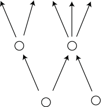
Figure 2: A typical graph where there are side branches entering the tree from the starting point. The $N_{\rm in}$ of the right node in the second layer should be 1 instead of 2, if we are interested in computing averages across the tree of nodes accessible from only the left starting point.

Because we are counting the number of bases one can get from blowing up the starting point, one should only count the $N_{\rm in}(a_{k})$ of a node for the blown down bases $b_{k-1}$ of $a_{k}$ that can be contracted to the starting point by a sequence of blow downs. This new $N^{\prime}_{\rm in}(a_{k})$ is always smaller or equal than $N_{\rm in}(a_{k})$. The discrepancy between $N^{\prime}_{\rm in}(a_{k})$ and $N_{\rm in}(a_{k})$ depends upon both the number of possible other starting point bases (bases that do not admit a smooth blow down) that connect to the graph after blowing up, and also upon the degree of connectivity of the graph. If the total number of possible starting points is order one, or much smaller than the total number of bases — as it is in six dimensions, where only the Hirzebruch surfaces and $\mathbb{P}^{2}$ are minimal starting points — then the estimation of the total number of bases in the ensemble should be reasonably accurate for one or more of the starting point bases. If, however, the number of minimally contracted bases is very large, this can lead to a dramatic underestimate of the total number of bases using this algorithm. Even if the number of possible starting bases is large, however, it only causes a significant problem with counting if a large fraction of the incoming edges to the nodes $a_{k}$ reached from blowing up $a_{1}$ lead only to other starting points besides $a_{1}$.

Focusing on the latter issue of connectivity, we can try to make a simple estimate of $N^{\prime}_{\rm in}(a_{k})$ by checking for each possible blow down whether the contracted ray is one of the rays on the starting point base or not. If it is not one of them, then we can add it into an estimated value $\tilde{N}^{\prime}_{\rm in}(a_{k})$, but otherwise we do not. The motivation for dropping these contractable rays is that if we contract one of the rays on the starting point, then in general the base may no longer contain a set of rays that are linearly equivalent to the set of rays on the starting point by an $SL(3,\mathbb{Z})$ transformation. It is possible, however, that after we contract a ray that corresponds to a ray on the starting point, there may still exist another configuration of the starting base somewhere else to which the base may be contracted. Hence this estimated $\tilde{N}^{\prime}_{\rm in}(a_{k})$ may be smaller than the actual value $N^{\prime}_{\rm in}(a_{k})$. On the other hand, there can also be bases that still include the rays of the starting point base $a_{1}$ but cannot be contracted to $a_{1}$ for other reasons; these will cause $\tilde{N}^{\prime}_{\rm in}$ to overestimate $N^{\prime}_{\rm in}$. As we see in the next section, the distinction between $N_{\rm in}$ and $\tilde{N}^{\prime}_{\rm in}$ amounts to a fairly minor difference in numerical results in the one-way Monte Carlo computations, so this crude estimation does not detect any significant under or overcounting due to a misestimation of $N^{\prime}_{\rm in}$. On the other hand, as we discuss in more detail in Section 5, it seems that there are many other starting point bases possible at large $h^{1,1}(B)$ that are “dead ends” reached when we blow down along random incoming edges of the $N_{\rm in}$ possibilities for $a_{k}$, so that both $N_{\rm in}$ and $\tilde{N}^{\prime}_{\rm in}$ are likely substantially over estimating the correct value $N^{\prime}_{\rm in}$ that would need to be used to correctly determine the number of nodes in the graph.

Finally, there is one further issue in this one-way Monte Carlo approach that results in a smaller estimation of the total number of bases, even if there are no additional starting points possible or additional edges entering the tree. While in principle the estimate (3.5) gives an accurate estimate of the number of nodes when carried out over many runs of the one-way Monte Carlo, this estimate may only be accurate when enough runs are done to completely explore the set of possibilities, which is practically impossible as the number of trajectories through the graph grows exponentially in $k$. In practice, the most probable branches of the blow-up tree that we enter are the ones with small weight factors, which lead to a small estimated number of $N_{\rm nodes}$ and $N_{\rm good}$. As an example, consider the red branch shown in Figure 3. If we only do one random blow up sequence through this graph, then we have a 60% possibility to enter this branch or the other two branches besides it. Applying (3.7) repeatedly along this path, we get that the estimation of the number of nodes in the top layer is given by the weight factor $D=5/27$ rather than 1. Thus, most of the time a random blow-up algorithm on this graph would give an expected number of nodes of $<0.2$ at the top level. This is compensated by low-probability paths with large weight; for example, the path along the left side of the graph has probability $0.1$ but gives a weight factor $D=10/3$. While indeed one can check that the expectation value over all paths in this graph is indeed $\langle D\rangle=1$, in a larger graph, such as one composed of many iterated copies of this graph, the distribution of $D$ values becomes highly asymmetric, and typical paths will give much lower values of $D$ than the idealized average. For graphs with a simple regular structure, such as an iterated version of the graph in Figure 3, this systematic underestimate can be compensated for by observing that the distribution of $D$’s takes a lognormal form. An example of how this can be corrected for in the case of a simple toy model is worked out in detail in Appendix A. Because the graph of connected threefold toric bases that we are exploring does not have a simple regular structure, it is unclear to what extent we can systematically compensate for this effect, but as we discuss in the following section this may be possible at least for local perturbations around a given trajectory.

To summarize the situation, there are several reasons why the approximation methods described in the previous subsection can give a systematic underestimate of the total number of nodes that can be reached by sequential blow-ups of a given toric threefold base $a_{1}$. We have not identified a clear and simple way of accurately compensating for the systematic underestimates just described, so the results presented here should be taken as lower bounds, with a more accurate estimation requiring an improved methodology for dealing with incoming branches such as in Figure 2 or the effect of more likely branches as in Figure 3. We will discuss this issue further in Section 4.4 in the context of the experimental data.

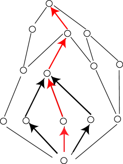
Figure 3: An example of a common branch in a random graph. Only from the information of $N_{\rm out}$ and $N_{\rm in}$ along this branch, we get a substantially underestimated total number of nodes in the top layer: $\frac{5}{27}$

4 Results

4.1 Blowing up $\mathbb{P}^{3}$

We have done 2,000 random blow up sequences starting from $\mathbb{P}^{3}$. We plot $\tilde{h}^{3,1}(X)$ of a generic elliptic fourfold over the base $B$ (see (2.2)) for some example blow up sequences as a function of $h^{1,1}(B)$ in Figure 4. As we can see, the number of Weierstrass moduli quickly drops to a very small number after about 50 blow ups.

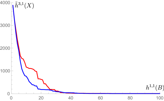
Figure 4: The change in $\tilde{h}^{3,1}(X)$ as a function of $h^{1,1}(B)$ for two random blow up sequences. The number of Weierstrass moduli drops quickly.

The sequences terminate after somewhere between 3,000 and 13,000 individual blow ups. We summarize the results of this numerical experiment, beginning with the set of good bases encountered and then addressing the estimation of the number of nodes in the full graph using the methods described in the previous section.

4.1.1 Good bases and end points

In the first 20 steps of the blow-up trajectory, many of the sequences encounter “good” bases without codimension-two (4, 6) loci. After this, all the sequences developed codimension-two (4, 6) toric curves, which continue to dominate the base geometry until the process converges at a terminal “end point” base that cannot be blown up further, which as discussed above is always “good”. An interesting feature of the results of this computation is that the Hodge numbers of the good end point bases appear to be clustered at certain specific isolated values, with some geometric significance.

We list the unweighted number of good bases $n_{\rm good}$ encountered among the 2,000 runs at each level $k$, with $h^{1,1}(B)=k$, in Table 2. This gives some estimation of the probability of finding a specific end point base from a random sequence. For those values with $h^{1,1}(B)<20$, the good bases encountered arise near the beginning of the blow-up sequence, and these are never terminal end point bases. The number of good bases decreases when $h^{1,1}(B)$ increases, since codimension-two (4,6) loci appear during the blow up process. The remaining good bases arise as end points. These have very large $h^{1,1}(B)$ and are concentrated at sporadic values of $h^{1,1}(B)$.

$h^{1,1}(B)$	$n_{\rm good}$	$h^{1,1}(B)$	$n_{\rm good}$	$h^{1,1}(B)$	$n_{\rm good}$	$h^{1,1}(B)$	$n_{\rm good}$
1	2000	2	2000	3	2000	4	1900
5	1645	6	1259	7	846	8	545
9	283	10	129	11	48	12	26
13	13	14	8	15	4	16	1
1317	1	1727	17	1799	4	1882	1
1943	198	2015	41	2047	23	2057	139
2186	44	2199	10	2249	315	2303	306
2395	10	2399	31	2491	6	2591	205
2599	17	2623	64	2636	6	2661	29
2821	4	2824	16	2891	1	2915	2
2943	1	2961	21	2999	40	3037	9
3071	3	3086	112	3157	1	3247	2
3276	4	3295	2	3374	4	3401	4
3422	34	3498	3	3539	2	3599	2
3658	12	3686	55	3739	1	3741	2
3789	1	3811	3	3817	1	3887	27
3992	1	4049	4	4211	1	4274	1
4373	25	4375	3	4394	21	4468	4
4520	1	4741	1	4748	1	4913	5
4939	10	4946	1	5143	21	5356	1
5383	5	5503	2	5522	1	5623	1
5878	1	5989	6	6143	2	6440	2
6784	1	6802	5	6911	8	6945	1
7373	1	7498	2	7526	1	7909	7
8111	3	8230	1	8435	1	8938	1
8980	5	8999	1	10124	3	11341	2
12631	1	-	-	-	-	-	-

Table 2: The number of good bases encountered for each $h^{1,1}(B)$ among the 2,000 runs, without counting the weight factor. Bases at small $h^{1,1}(B)<20$ are not end points, all bases with large $h^{1,1}(B)>1000$ are end points of the algorithm.

One can see from Table 2 that for bases with $h^{1,1}(B)\leq 3$, all bases are good. Indeed an explicit analysis by hand shows that only blowing up two points or curves is insufficient to generate a codimension-two (4, 6) locus. As $h^{1,1}(B)$ increases above $k=3$, the number of good bases among the 2,000 runs decreases quickly, because there are an increasing number of ways to generate bases with codimension-two (4,6) loci after a number of blow ups.

The other set of good bases encountered in the runs is the set of scattered end points with $h^{1,1}(B)>1,000$, whose number indeed adds up to 2,000, as one can check explicitly. While some $h^{1,1}(B)$ only arise as the end points of one or a few runs, there are sharp spikes in the distribution associated with particular values that arise frequently; of the 2,000 runs, the number of distinct values of $h^{1,1}(B)$ at the endpoint is only 89. It is interesting to study the structures of the bases at the most prominent spikes, for example $h^{1,1}(B)=1943$, 2249, 2303 and 2591, each of which arises for roughly 10% or more of the blow-up trajectories. It turns out that for all the end point bases we found with each specific value of $h^{1,1}(B)$, the non-Higgsable gauge group contents are the same. For $h^{1,1}(B)=1943$, 2249, 2303 and 2591, the gauge groups are $G=E_{8}^{29}\times F_{4}^{81}\times G_{2}^{216}\times SU(2)^{324}$, $E_{8}^{33}\times F_{4}^{94}\times G_{2}^{250}\times SU(2)^{375}$, $E_{8}^{34}\times F_{4}^{96}\times G_{2}^{256}\times SU(2)^{384}$ and $E_{8}^{38}\times F_{4}^{108}\times G_{2}^{288}\times SU(2)^{432}$ respectively. This general structure is a common feature of the end point bases, since $f$ almost always vanishes to degree 4 on every divisor (i.e. $\mathcal{F}=\{(0,0,0)\}$), so that the most common non-Higgsable gauge group factors will be SU(2), $G_{2}$, $F_{4}$ and $E_{8}$, corresponding to the cases where $g$ vanishes to degree 2,3,4 and 5 respectively. (This same structure arises for elliptic Calabi-Yau threefolds over base surfaces, where at large $h^{1,1}(B_{2})$ the geometry is dominated by “$E_{8}$ chains” containing the non-Higgsable clusters $-12,-5$, and $(-3,-2)$, which carry the gauge groups $E_{8},F_{4}$, and $G_{2}\times SU(2)$ respectively [6, 7].) The gauge groups SU(3) and SO(8) also appear in some places, but infrequently; for example the bases with $h^{1,1}=2999$ have gauge groups $E_{8}^{44}\times F_{4}^{125}\times G_{2}^{332}\times SU(3)\times SU(2)^{500}$. An empirical formula for the number of gauge group factors SU(2), $G_{2}$, $F_{4}$ and $E_{8}$ in terms of $h^{1,1}(B)$ goes roughly as

$$N_{SU(2)}\cong\left[\frac{h^{1,1}(B)+1}{6}\right]\ ,\ N_{G_{2}}\cong\left[\frac{h^{1,1}(B)+1}{9}\right]\ ,\ N_{F_{4}}\cong\left[\frac{h^{1,1}(B)+1}{24}\right]\ ,\ N_{E_{8}}\cong\left[\frac{h^{1,1}(B)}{68}\right].$$ (4.1)

While the non-Higgsable gauge groups appear to be quite uniform across end points with common $h^{1,1}(B)$, the non-Higgsable cluster structures on the bases with the same $h^{1,1}(B)$ are very different; this can be easily checked by looking at the different total number of non-Higgsable clusters and their different sizes. These bases also can have different convex hulls of the fan, hence they are not always related by a series of flops.

A potentially very interesting finding is that the Hodge numbers of the elliptic Calabi-Yau fourfolds associated with end point bases at large $h^{1,1}(X)$ seem to give the mirror Hodge numbers to those of various generic elliptically fibered Calabi-Yau fourfolds over bases with small $h^{1,1}(B)$. For example, some of the bases with $h^{1,1}(B)=2303$ give $h^{1,1}(X)=3878$ and $h^{3,1}(X)=2$. Since a generic elliptic fibration over $\mathbb{P}^{3}$ gives an $X$ with $h^{1,1}(X)=2$ and $h^{3,1}(X)=3878$, these look exactly like mirror Calabi-Yau fourfold pairs. There are also other bases with $h^{1,1}(B)=2303$ that give $h^{1,1}(X)=3877$ and $h^{3,1}(X)=4$. They are also included in the dataset of Calabi-Yau fourfolds constructed as hypersurfaces in weighted projective space using reflexive polytopes [42]. For the bases with $h^{1,1}(B)=1943$, the generic elliptic Calabi-Yau fourfold has $h^{1,1}(X)=3277$ and $h^{3,1}(X)=3$, which exactly looks like the dual of a generic elliptic fibration over the generalized Hirzebruch threefold $\tilde{\mathbb{F}}_{0}$, which is $\mathbb{P}_{1}\times\mathbb{P}_{2}$. We list many of these interesting cases in Table 3. In this table, the generalized Hirzebruch threefold $\tilde{\mathbb{F}}_{n}$ is a $\mathbb{P}_{1}$ bundle over $\mathbb{P}_{2}$ with total twist $n$. In toric language, the 1D rays in the fan are $v_{1}=(1,0,0),v_{2}=(0,1,0),v_{3}=(0,0,1),v_{4}=(0,0,-1)$ and $v_{5}=(-1,-1,-n)$. The 3D cones in the fan are $\{v_{1}v_{2}v_{3},v_{1}v_{5}v_{3},v_{2}v_{5}v_{3},v_{1}v_{2}v_{4},v_{1}v_{5}v_{4},v_{2}v_{5}v_{4}\}$. Note that in other cases the end point bases support elliptic Calabi-Yau fourfolds that seem to be dual to other Calabi-Yau fourfolds with small $h^{1,1}(X)$ but that are not elliptically fibered. For example, the bases with $h^{1,1}(B)=2249$ give Calabi-Yau fourfolds with $h^{1,1}(X)=3786$ and $h^{3,1}(X)=2$, which is also in the database [42], but there is no other threefold base besides $\mathbb{P}^{3}$ with $h^{1,1}(B)=1$, so there are no other elliptic Calabi-Yau fourfolds with $h^{1,1}(X)=2$ besides the generic elliptic fibration over $\mathbb{P}^{3}$, and the dual Calabi-Yau in this case it seems is not a simple elliptic fibration.

$h^{1,1}(B)$ (toric)	gauge group	$h^{1,1}(X)$	$h^{3,1}(X)$	Mirror base
1943	$E_{8}^{29}\times F_{4}^{81}\times G_{2}^{216}\times SU(2)^{324}$	3277	3	$\tilde{\mathbb{F}}_{0}$
2015	$E_{8}^{30}\times F_{4}^{84}\times G_{2}^{224}\times SU(2)^{336}$	3397	3	$\tilde{\mathbb{F}}_{1}$
2303	$E_{8}^{34}\times F_{4}^{96}\times G_{2}^{256}\times SU(2)^{384}$	3878	2	$\mathbb{P}^{3}$
2591	$E_{8}^{38}\times F_{4}^{108}\times G_{2}^{288}\times SU(2)^{432}$	4358	3	$\tilde{\mathbb{F}}_{3}$
3086	$E_{8}^{45}\times F_{4}^{129}\times G_{2}^{343}\times SU(2)^{513}$	5187	4	$\tilde{\mathbb{F}}_{4}$
3686	$E_{8}^{54}\times F_{4}^{153}\times G_{2}^{409}\times SU(2)^{615}$	6191	5	$\tilde{\mathbb{F}}_{5}$
4373	$E_{8}^{64}\times F_{4}^{180}\times SO(8)\times G_{2}^{486}\times SU(2)^{729}$	7341	7	$\tilde{\mathbb{F}}_{6}$
5143	$E_{8}^{75}\times F_{4}^{213}\times G_{2}^{571}\times SU(2)^{858}$	8629	7	$\tilde{\mathbb{F}}_{7}$
5989	$E_{8}^{87}\times F_{4}^{249}\times G_{2}^{664}\times SU(2)^{999}$	10045	7	$\tilde{\mathbb{F}}_{8}$
10124	$E_{8}^{145}\times F_{4}^{423}\times G_{2}^{1125}\times SU(2)^{1683}$	16959	10	$\tilde{\mathbb{F}}_{12}$
11341	$E_{8}^{162}\times F_{4}^{474}\times G_{2}^{1261}\times SU(2)^{1887}$	18994	12	$\tilde{\mathbb{F}}_{13}$
12631	$E_{8}^{180}\times F_{4}^{528}\times G_{2}^{1405}\times SU(2)^{2103}$	21151	12	$\tilde{\mathbb{F}}_{14}$

Table 3: A list of end point bases with the feature that the generic elliptic fibration over the base gives a Calabi-Yau fourfold with interesting Hodge numbers. In these cases the fourfolds seem to form mirror pairs with generic elliptic Calabi-Yau fourfolds over simple “mirror bases” with small $h^{1,1}(B)$. The $h^{1,1}(B)$ listed in the first column means the $h^{1,1}(B)$ of the toric base before the codimension-two (4,6) loci on divisors with $E_{8}$ are blown up.

It is hard to directly prove that these Calabi-Yau fourfolds with large $h^{1,1}$ are actually the mirrors of the Calabi-Yau fourfolds with small $h^{1,1}$ and large $h^{3,1}$, because the Calabi-Yau fourfolds over specific threefold bases with large $h^{1,1}$ are generally hard to realize explicitly as hypersurfaces in reflexive polytopes. It is natural that the Calabi-Yau fourfolds with the same Hodge numbers could be isomorphic to each other. But it is still an open question how to check this isomorphism.

4.1.2 Approximating the total number of resolvable and good bases

Given the results of the 2,000 one-way Monte Carlo runs starting from $\mathbb{P}^{3}$, we can try to estimate the total number of resolvable and good bases that can be reached as blow-ups of $\mathbb{P}^{3}$ using (3.1), (3.5) and (3.8).

For each run of the one-way Monte Carlo, the dynamic weight $D(n)$ given by (3.1) gives an estimate of the total number of accessible nodes at level $n$. We can write this as

$$D(n)=\prod_{i=1}^{n-1}d_{k},\;\;\;\;\;d_{k}=\frac{N_{\rm out}(a_{k})}{N_{\rm in}(a_{k+1})}\,.$$ (4.2)

To get a sense of the overall shape of the graph, we plot in Figure 5 the value of

$$\log_{10}(d_{k})\equiv\log_{10}\left(\frac{N_{\rm out}(a_{k})}{N_{\rm in}(a_{k+1})}\right)$$ (4.3)

at each layer $k$ for three specific random sequences, which end at $h^{1,1}=4373$, 3498 and 2249 respectively. Note that

$$\log_{10}D(n)=\sum_{i=1}^{n-1}\log_{10}d_{k}\,.$$ (4.4)

One can see that for each run there is a specific value $k=k^{\star}$ where $\log_{10}(d_{k})$ changes sign. That location of $k$ will correspond to the maximal value of the weight factor $D({k^{\star}})$ along a particular trajectory through the graph, which varies with the trajectory. For small $k$, the weight factor from (4.2) will grow roughly exponentially, until as $k$ reaches $k^{\star}$ on a given trajectory the weight factor peaks and begins to go down.

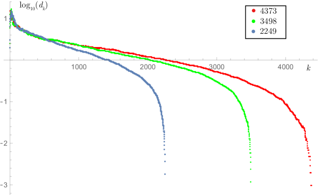
Figure 5: The plot of $\log_{10}(d_{k})=\log_{10}\left(\frac{N_{\rm out}(a_{k})}{N_{\rm in}(a_{k+1})}\right)$ for each node $a_{k}$ in each layer $k$ for three random blow-up sequences, whose end points are $h^{1,1}(B)=4373$, 3498 and 2249 respectively.

Combining the different runs, we can compute the average value of $D(n)$ at each $n$ using (3.5), which gives the expected number of resolvable bases, and the number of good bases can be estimated as discussed following equation (3.8) by using (3.5) with a 0 contribution to $D$ for any trajectory that does not reach a good base at level $n$. We plot the logarithm of the estimated number of resolvable bases and good bases in Figure 6 and Figure 7 respectively. As one may expect, the number of resolvable bases varies smoothly. As we have discussed above, however, the distribution of good bases consists of spikes. Because the weight factor has a large exponent, and as seen in Figure 5 the $k$-dependence of $d_{k}$ varies fairly widely between runs, the distribution of resolvable bases is dominated by the trajectory with the largest value of $k^{*}$, while the distribution of good bases is a sum from the spikes of the different end point bases.

Figure 6: Logarithm of the estimated number of resolvable bases $N_{\rm nodes}$ as function of $h^{1,1}(B)$, from blowing up $\mathbb{P}^{3}$.

Figure 7: Logarithm of the estimated number of good bases $N_{\rm good}$ as function of $h^{1,1}(B)$, from blowing up $\mathbb{P}^{3}$.

We can see from the figure that when $h^{1,1}(B)>5,000$, the estimated number of good bases with that $h^{1,1}(B)$ is significantly smaller than 1, even though we found some good end point bases with much larger values of $h^{1,1}(B)$. Moreover, the estimated number of resolvable bases is smaller than 1 at $h^{1,1}(B)>11,000$. For example, for the base with biggest $h^{1,1}(B)=12,631$, the total number of bases is estimated as $2.2\times 10^{-2474}$. This fact verifies that we have indeed underestimated the total number of bases by a large exponential factor. Typically there are $\sim 10^{3}$ incoming edges for the bases near the end points but only a few outgoing edges, hence the situation is more extreme than Figure 3 shows.

Using the uncorrected $N_{\rm in}(a_{k})$ in (3.1), the estimated total number of resolvable bases is equal to $3.5\times 10^{1964}$ and the estimated number of good bases equals to $3.0\times 10^{253}$. If we use the corrected estimation $\tilde{N}^{\prime}_{\rm in}(a_{k})$ as discussed in Section 3.2.3, then the total number of resolvable bases is again estimated at to $3.5\times 10^{1964}$ and the number of good bases is estimated at $9.1\times 10^{253}$. Hence from the experimental results, it seems that the different definition between $\tilde{N}^{\prime}_{\rm in}(a_{k})$ and $N_{\rm in}(a_{k})$ does not much affect the estimation, so this mechanism does not capture the source of the underestimation. We discuss the reasons for the underestimation and possible corrections further in Section 4.4.

Note that even with the underestimation error, it is clear that the set of resolvable bases that can be constructed through this approach is significantly larger than the $10^{755}$ bases found in [29]. We can relate these computations in terms of the possible “heights” of divisors $h(D_{i})$ used in that paper. We assign a number 1 to each divisor on the starting point $\mathbb{P}^{3}$. Whenever we blow up a 3D cone $D_{i}D_{j}D_{k}$, we assign a number $h(E)=h(D_{i})+h(D_{j})+h(D_{k})$ to the exceptional divisor. Similarly, if we blow up a 2D cone $D_{i}D_{j}$, we assign a number $h(E)=h(D_{i})+h(D_{j})$ to the exceptional divisor. In [29] they use a sufficient criterion that the height of any divisor on a base cannot exceed 6 in order to avoid codimension-one (4,6) loci. However, in our Monte Carlo algorithm, the typical maximal height of a divisor on an end point ranges from 50–350, which drastically exceeds the limit 6.

4.2 Blowing up other starting points with small $h^{1,1}(B)$

To cross-check the results in the previous section, we have also looked at blow-up trajectories from other starting point bases with small $h^{1,1}(B)$.

Two other starting bases we have tried are the generalized Hirzebruch threefold $\tilde{\mathbb{F}}_{2}$ with $h^{1,1}(B)=2$ and a simple product space $\mathbb{P}^{1}\times\mathbb{P}^{1}\times\mathbb{P}^{1}$ with $h^{1,1}(B)=3$. Similar to $\mathbb{P}^{3}$, these bases do not have non-Higgsable gauge groups. After 1,000 random blow up sequences starting from $\tilde{\mathbb{F}}_{2}$, we found a larger fraction of end point bases with large $h^{1,1}(B)$ than when starting from $\mathbb{P}^{3}$. For $\tilde{\mathbb{F}}_{2}$, 1% of end points have $h^{1,1}(B)>10,000$, while this percentage is 0.3% from the starting point $\mathbb{P}^{3}$. The largest $h^{1,1}(B)$ we got is 20,341, and the non-Higgsable gauge group on the resulting good endpoint base is $E_{8}^{290}\times F_{4}^{850}\times G_{2}^{2261}\times SU(2)^{3383}$. We estimate the total number of resolvable bases from $\tilde{\mathbb{F}}_{2}$ at $1.24\times 10^{3046}$ while the total number of good bases is estimated at $1.10\times 10^{254}$, using weight factors with $N^{\prime}_{\rm in}(a_{k})$. On the other hand, after 1,000 random blow up sequences from $\mathbb{P}^{1}\times\mathbb{P}^{1}\times\mathbb{P}^{1}$, the total number of resolvable bases is estimated to be $1.43\times 10^{1811}$ and the total number of good bases is estimated to be $1.80\times 10^{271}$.

We plot the distribution of resolvable bases and good bases from the three starting points in Figures 8 and  9 respectively.

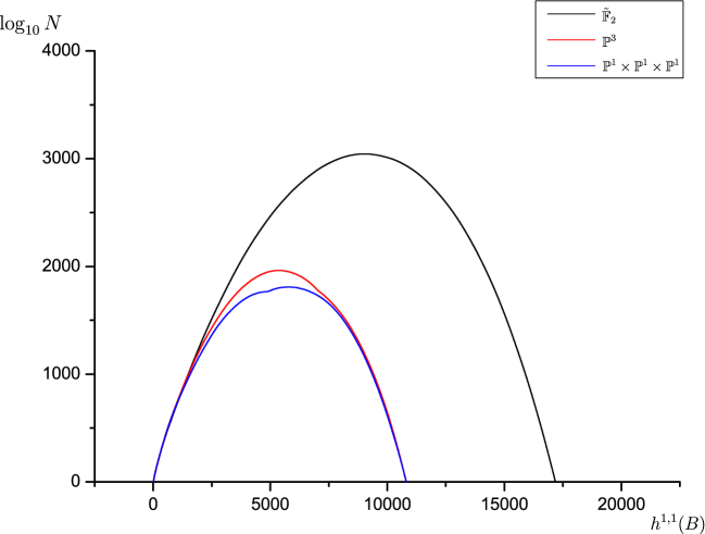
Figure 8: Logarithm of the estimated number of resolvable bases as function of $h^{1,1}(B)$ from blowing up $\mathbb{P}^{3}$, $\tilde{\mathbb{F}}_{2}$ and $\mathbb{P}^{1}\times\mathbb{P}^{1}\times\mathbb{P}^{1}$.

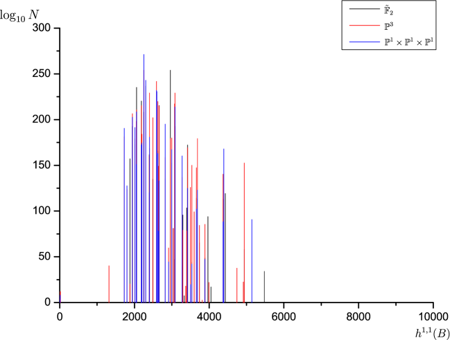
Figure 9: Logarithm of the estimated number of good bases as function of $h^{1,1}(B)$ from blowing up $\mathbb{P}^{3}$, $\tilde{\mathbb{F}}_{2}$ and $\mathbb{P}^{1}\times\mathbb{P}^{1}\times\mathbb{P}^{1}$.

Many peaks in Figure 9 indeed overlap between starting points; for example, the total number of good bases with $h^{1,1}(B)=2249$, 2303, 2591, 2961 and 2999 for the starting points ($\mathbb{P}^{3}$,$\mathbb{F}_{2}$,$\mathbb{P}^{1}\times\mathbb{P}^{1}\times\mathbb{P}^{1}$) are on the order of $(10^{254},10^{208},10^{271})$, $(10^{211},10^{236},10^{243})$, $(10^{241},10^{161},10^{232})$, $(10^{179},10^{254},10^{-227})$ and $(10^{180},10^{152},10^{167})$ respectively. The highest peaks from the starting points ($\mathbb{P}^{3}$,$\mathbb{F}_{2}$,$\mathbb{P}^{1}\times\mathbb{P}^{1}\times\mathbb{P}^{1}$) locate at $h^{1,1}(B)=(2249,2961,2249)$ respectively. Because of the big exponential error on these estimations, we cannot fix the exact peak in the distribution of good bases, and these numbers are clearly not very accurate estimates. We discuss some related issues further in Section 5

Similar to the runs from $\mathbb{P}^{3}$, the total number of bases with large $h^{1,1}(B)$ seems to be hugely underestimated. Starting from $\tilde{\mathbb{F}}_{2}$, we get an extremely small estimation $6\times 10^{-4221}$ for the number of bases with $h^{1,1}(B)=20,341$. Starting from $\mathbb{P}^{1}\times\mathbb{P}^{1}\times\mathbb{P}^{1}$, we find that the total number of bases with $h^{1,1}(B)=12,631$ is estimated at $5\times 10^{-2454}$. Since in both cases the actual number must be at least 1, we may roughly expect that the error in the exponent grows linearly with $k$, so that the true number of bases may be closer to $10^{6000}$ than the underestimate $10^{3000}$, though more careful analysis would be needed to nail down this number more precisely.

As another starting point with somewhat different structure, we have also tried blowing up starting with the generalized Hirzebruch threefold $\tilde{\mathbb{F}}_{12}$, which has $h^{1,1}(B)=2$ and a non-Higgsable gauge group $E_{7}$. Despite the existence of an $E_{7}$, the Weierstrass model does not suffer from the problem of codimension-three (4,6) loci and non-flat fibration described in Section 2, because the coefficient $b_{0}$ in (2.10) cannot vanish. After 100 random blow up sequences, the total number of resolvable bases is estimated as $1.77\times 10^{2130}$ while the total number of good bases is estimated as $2.02\times 10^{7}$.

The distribution of $h^{1,1}(B)$ among the 100 runs starting from $\tilde{\mathbb{F}}_{12}$ has a greater preference towards large $h^{1,1}(B)$ than the other starting points we have investigated. 17% of end point bases have $h^{1,1}(B)>10,000$, and the largest $h^{1,1}(B)$ we found is $33,021$. Nonetheless, we can still find 1 base with $h^{1,1}(B)=2249$, 4 bases with $h^{1,1}(B)=2303$ and 8 bases with $h^{1,1}(B)=2591$, which are common bases in Table 2. Another interesting phenomenon is that none of the end point bases has an $E_{7}$ gauge group factor. The divisor possessing an $E_{7}$ gauge group at the starting point always has an $E_{8}$ at the end point instead.

4.3 Blowing up the base $B_{\rm max}$ that gives rise to the elliptic CY fourfold $\mathcal{M}_{\rm max}$ with the largest $h^{3,1}$

In [43], we explicitly constructed the base $B_{\rm max}$ such that the generic elliptic CY fourfold $\mathcal{M}_{\rm max}$ over it has the largest $h^{3,1}$: $(h^{1,1},h^{3,1})=(252,303148)$. This is the largest value of $h^{3,1}$ known for any Calabi-Yau fourfold, elliptic or not. As argued in [43], we believe this should be the largest possible value for any elliptic Calabi-Yau fourfold, but unlike the analogous maximum value of $h^{2,1}(X_{3})=491$ for elliptic Calabi-Yau threefolds [7], we do not have a rigorous proof of the upper bound for fourfolds. The base $B_{\rm max}$ is constructed as a $B_{2}$ bundle over $\mathbb{P}^{1}$, where $B_{2}$ is a toric surface characterized by a closed cycle of toric curves with self-intersections $0,+6,$ -12//-11//-12//-12//-12//-12//-12//-12//-12, where $//$ denotes the “$E_{8}$ chain” of self-intersections $-1,-2,-2,-3,-1,-5,-1,-3,-2,-2,-1$. The generic elliptic CY threefold over $B_{2}$ is a self-mirror CY3 with Hodge numbers $(251,251)$ [6, 7]. The toric rays $w_{i}$ on $B_{2}$ can be choosen to be

$$w_{1} = (-1,-12)$$ (4.5)

$$w_{2} = (0,1)$$ (4.6)

$$w_{3} = (1,6)$$ (4.7)

$$\vdots \vdots$$ (4.8)

$$w_{99} = (0,-1)\,.$$ (4.9)

The intermediate rays can be determined by the condition $w_{i-1}+w_{i+1}+(C_{i}\cdot C_{i})w_{i}=0$, where $C_{i}\cdot C_{i}$ is the self-intersection of the $i$th curve. From the rays $w_{i}$ we can construct the toric fan for $B_{\rm max}$, which is given by the rays

$$v_{0} = (0,0,1)$$ (4.10)

$$v_{i} = (w_{i},0),\;\;\;\;\;1\leq i\leq 99$$ (4.11)

$$v_{100} = (84,492,-1)=(12w_{15},-1)\,,$$ (4.12)

where $C_{15}$ is the curve in $B_{2}$ of self-intersection $-11$. The 3D cones of the fan for $B_{\rm max}$ are given by $(v_{0},v_{i},v_{i+1})$ and $(v_{100},v_{i},v_{i+1})$, including the ones $(v_{0}/v_{100},v_{99},v_{1})$.

We performed 100 random blow up sequences from $B_{\rm max}$, getting 100 endpoints with $h^{1,1}(B)=2636-16103$. The total number of resolvable bases is estimated at $1.14\times 10^{520}$ while the total number of good bases is $4.3\times 10^{4}$, which is an extremely small number. This is a common feature of this Monte Carlo approach when one starts from bases with large non-Higgsable gauge groups, and we can conclude that the number of bases we can get by blowing up bases with larger $h^{1,1}(B)$ is significantly smaller than the number of bases we can get by blowing up $\mathbb{P}^{3}$. This matches with what we expect from the case of base surfaces where the complete set of toric bases is known.

It is notable that although the structure of $B_{\rm max}$ looks completely different from $\mathbb{P}^{3}$, 42% of the end point bases we get from blowing up $B_{\rm max}$ have $h^{1,1}(B)$ that can be found in Table 2. For example, 7% of bases have $h^{1,1}(B)=7909$ and 5% of bases have $h^{1,1}(B)=8980$. This implies that the end point bases from different starting points have a large overlap, and the ensemble of bases we get from blowing up $\mathbb{P}^{3}$ may be a decent 0th order approximation to the total set of 3D toric bases.

Another interesting challenge is to find a blow-up sequence to explicitly generate the base $B$ with the largest value of $h^{1,1}(B)$, which gives rise to the elliptic fourfold $X$ with the largest $h^{1,1}(X)$. In the lower dimensional (base surface) case, we know that the generic elliptic Calabi-Yau threefold over $\mathbb{F}_{12}$ has Hodge numbers $(h^{1,1},h^{2,1})=(11,491)$. If one blows it up, the “end point” bases include one with $h^{1,1}(B)=174$, which gives rise to the Calabi-Yau threefold with $(h^{1,1},h^{2,1})=(491,11)$. These two Calabi-Yau threefolds are the currently known (irreducible) Calabi-Yau threefolds with the largest $h^{2,1}$ and $h^{1,1}$ respectively. So if we start from the base $B_{\rm max}$ and blow it up, requiring that the number of complex structure moduli is maximized at each step, we may expect to finally reach a base with the largest $h^{1,1}(B)$ that gives rise to the mirror fourfold of $\mathcal{M}_{\rm max}$, with $(h^{1,1},h^{3,1})=(303148,252)$ [40]. But it is quite time consuming to actually perform such a search, since one has to enter a region where typical bases have $\mathcal{O}(100,000)$ rays and $\mathcal{O}(100,000)$ complex structure moduli; we leave the resolution of this challenge to future work.

4.4 Systematic error of the estimated total number

As we have mentioned before, the number of bases at large $h^{1,1}(B)$ tends to be substantially underestimated by using the weight factor through (3.5). For example, the weight factor suggests that for the starting point $\tilde{\mathbb{F}}_{2}$, the total number of bases with $h^{1,1}(B)>20,000$ is something like $10^{-4000}$. Not only do we know that there is at least one base in this range, but there is actually a large multiplicity of such bases.

We can get a rough estimate of the multiplicity of bases at the large Hodge numbers where there are good end points by considering flops. In general, for many of the bases we encounter we know that there exist a large number of flop operations on the base which transform it to another base with the same rays but a different cone structure. Such a flop appears when there are rays $v_{i},v_{j},v_{k},v_{l}$ satisfying the relation $v_{i}+v_{j}=v_{k}+v_{l}$, and there is a 2d cone $v_{i}v_{j}$, see Figure 10. When there are many rays on a face of the convex hull of the polytope formed from the base fan, there are generally many possible flops. For example, the number of possible flop operations on an end point base with $h^{1,1}(B)=10,124$ ranges from 3440 to 3980, and there are 7040 flops on an end point base with $h^{1,1}(B)=20,341$. In general, we can empirically estimate that the number of flops on an end point base scales linearly as $N_{flop}\approx 0.3h^{1,1}(B)$–$0.4h^{1,1}(B)$. As discussed in [28], a rough estimate for the number of distinct bases associated with a given base with $n$ flops is $2^{n}$. This implies that there are at least something like $\sim 2^{3500}\approx 10^{1000}$ bases with $h^{1,1}(B)=10,124$ and at least $\sim 2^{7000}\approx 10^{2000}$ bases with $h^{1,1}(B)=20,341$, just from the different combinations of flop operations on these bases. In the set of bases studied in [28], flops were not the primary source of multiplicity for bases with common Hodge numbers. Indeed, for the good end point base values of $h^{1,1}(B)$ encountered here, there are generally many bases with different set of rays that cannot be identified with flops. Thus, the number of different end point bases with $h^{1,1}(B)\gtrsim 10,000$ should be significantly larger than 1.

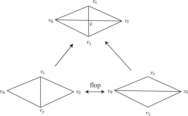
Figure 10: An illustration of the flop process, which can happen when $v_{i}+v_{j}=v_{k}+v_{l}$.

The underestimation of the number of bases at large $h^{1,1}(B)$ has two potential origins that we are aware of:

(1) The branches with highest probability will have a weight factor that is lower than the actual average weight factor, leading to a systematic exponential underestimate of the number of bases for typical blow-up trajectories. As in the toy model described in Appendix A, this effect can also produce an exponential suppression $e^{-ak}$ on the weight factor.

(2) We are overcounting $N_{\rm in}$ because for some of the bases $B$ that are generated by blowing up the starting point a number of times some of the incoming edges are associated with contractions to bases that cannot be contracted to the starting point through a sequence of smooth bases. This overcounting issue may occur at most levels of the blow-up process, which is likely to lead to a roughly exponential underestimation $e^{-bk}$ on the weight factor $D$.

Because both of these effects can have an exponential suppression of the weight factor it is important to distinguish their relative significance. We believe that the factor (2) is the primary cause of the underestimation, but we cannot quantify it precisely yet since it is difficult to tell whether a base can be contracted to $\mathbb{P}^{3}$ or not. This issue may be addressed by systematically understanding what fraction of incoming edges $N_{\rm in}$ can lead to a contraction back to the starting point, or potentially by systematically understanding the set of starting point bases that are either smooth or admit certain kinds of singularities. We discuss the two possible issues related to undercounting in turn, first by arguing that (1) is not the principal source of underestimation error, and then by making some simple observations on the existence of additional starting points relevant to (2).

4.4.1 Weight factors and the lognormal distribution

Problem (1) is illustrated with a toy model of a homogeneous random graph in Appendix A, where the actual number of nodes for each layer $k$ is constant, but the formula (3.5) will lead to an exponentially small number $D\propto e^{-ak}$ for typical blow-up trajectories, and the proper average is only restored by sampling exponentially unlikely trajectories. In this simple model, the logarithm of $D(k)/D(k-1)$ is essentially a random variable sampled independently at each level, so the distribution of weight factors $D$ at layer $k$ obeys a lognormal distribution and the standard deviation $\sigma$ of $\log_{10}(D)$ scales as $\sigma\propto\sqrt{k}$, while the mean $\mu$ of $\log_{10}(D)$ scales as $k$. In such a situation, we can compute the expectation value of the weight factor:

$$\begin{split}\langle D\rangle&=\int_{-\infty}^{\infty}e^{x\log 10}\cdot\frac{1}{\sqrt{2\pi\sigma^{2}}}e^{-\frac{(x-\mu)^{2}}{\sigma^{2}}}dx\\ &=\exp\left[\mu\log 10+\frac{\sigma^{2}(\log 10)^{2}}{2}\right].\end{split}$$ (4.13)

Typical trajectories will only see the first term, so there is a systematic underestimate of $D$ of the form $e^{-ak}$ that can be corrected by including the $\sigma^{2}$ term in the exponent by hand as a correction factor.

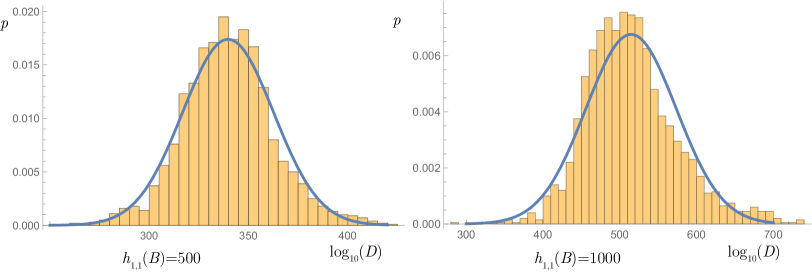
Figure 11: Distribution of the logarithm of the dynamic weight factor $D$ at $h^{1,1}(B)=500$ and 1,000 and the fitting curve using a normal distribution. For $h^{1,1}(B)=500$, the mean value of $\log_{10}(D)$ is 339.707 while the standard deviation is 22.9357. For $h^{1,1}(B)=1,000$, the mean value of $\log_{10}(D)$ is 514.694 while the standard deviation is 59.0485.

While this analysis is directly applicable for homogeneous graphs like the toy model in Appendix A, which have a structure that is identical at each level and homogeneous across the graph at each level, it is more subtle to use this kind of analysis for the graph of toric threefold bases sampled through successive blow-ups, which is different at each level and not homogeneous across trajectories that explore different parts of the graph. As a simple illustration of this distinction, we plot the distribution of the logarithm of the weight factors at $h^{1,1}(B)=500$ and 1,000 starting from $\mathbb{P}^{3}$ in Figure 11. We also fit the logarithm of weight factors $x=\log_{10}(D)$ using a normal distribution with mean value $\mu$ and standard deviation $\sigma$. It turns out that for this data, the standard deviation grows faster than $\sqrt{k}$, at least in some regime of values of $k$. Hence the actual distribution of $D$ cannot be approximated by the simple lognormal distribution arising from a product of equally distributed factors, as it can for the random graph toy model in the Appendix A.

An important distinction in the toric threefold blow-up graph is that each random blow-up sequence actually enters a separate region of the graph with different local statistics at a given level. This statement even holds for different branches that lead to the same end point. For example, we plot $\log_{10}(d_{k})=\log_{10}\left(\frac{N_{\rm out}(a_{k})}{N_{\rm in}(a_{k+1})}\right)$ of three different branches that lead to end points with $h^{1,1}(B)=2249$ in Figure 12. Since $D(a_{k})=\prod_{i=1}^{k-1}d_{i}$, the weight factor $D$ for the red branch at $k>1000$ will be significantly smaller than the $D$ for blue and green branches. Furthermore, the divergence between different branches, particularly those with different endpoints, leads to an extremely large standard deviation on $D$ when compared across paths. This would lead to an unreasonably large correction factor $e^{c\sigma^{2}}$ from the second term in the exponent of (4.13) if we naively assume a lognormal distribution.

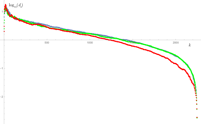
Figure 12: The plot of $\log_{10}(d_{k})=\log_{10}\left(\frac{N_{\rm out}(a_{k})}{N_{\rm in}(a_{k+1})}\right)$ for each node $a_{k}$ in each layer $k$ for three random blow up sequences, whose end points are bases with $h^{1,1}(B)=2249$.

Thus, it does not make sense to consider the full set of trajectories in the context of a lognormal distribution on $D$. Nonetheless, we may imagine that each trajectory follows a path where the local factor $d_{k}$ is chosen at each $k$ from some distribution such that the final distribution on $\log(D)$ can be described as the summation of the distributions on $\log(d_{k})$, which will again give a roughly lognormal form given the local distribution of $d_{k}$ factors in each region of the full graph traversed by a given trajectory. To estimate the effect in such a local model, we can compute the local variation or smoothness of the curve $f(k)\equiv\log_{10}(d_{k})$ for a single branch to roughly estimate the standard deviation responsible for the underestimation of type (1) along a particular trajectory. As described in Appendix A, we can compute the “local” standard deviation

$$\sigma(a_{k})=\sqrt{\frac{\sum_{i=k-l}^{k+l}\left(f(i)-\frac{1}{2l+1}\sum_{j=k-l}^{k+l}f(j)\right)^{2}}{2l+1}}$$ (4.14)

for each node $a_{k}$ and take the the standard deviation $\sigma$ in the compensation formula (4.13) to be

$$\sigma=\sqrt{\sum_{i=l+1}^{k-l}\sigma^{2}(a_{i})}.$$ (4.15)

Here $l$ can be an arbitrary positive integer with the condition $l\ll k$. A slightly more sophisticated analysis could take account of correlations between successive values of $f(k)$, but this would only serve to reduce the $\sigma^{2}$-based correction factor.

As an example of this local analysis, for the blue curve in Figure 12, if we take $l=4$, then the final standard deviation for $k=2249$ is $\sigma=0.683$, which is extremely small, and is essentially a negligible correction to the weight factor given the large apparent undercounting error in the exponent. This can be compared, for example, with the toy model in Appendix A, where there is an underestimation factor of $10^{-50}$ at $k=1000$, and the standard deviation is $\sigma=21.7307$. This analysis suggests that the unevenness of the weight factor due to local fluctuations in the structure of the graph in the vicinity of specific blow-up trajectories, i.e. explanation (1) above, is not the major cause of the exponentially small number $N_{\rm node}\propto e^{-ak}$.

4.4.2 Exotic smooth starting points

To investigate the question of whether some of the $N_{\rm in}$ incoming edges at a typical node $B$ may not lead down to a base that can be contracted to the starting point, a natural question that we can address is: what is the maximal number of blow downs we can perform with a random sequence starting at an end point base $B$ before reaching a starting point that cannot be contracted through a blow down to another smooth base. It turns out that after a random sequence of blow downs on a typical good end point base, we almost always hit a base with $h^{1,1}(B)=50$–$200$ that cannot be contracted to another smooth base, even if we require that the original rays on the starting point are never removed. These “exotic starting points” have a complicated fan structure. Most of the rays in the fan have more than four neighbors, hence this base is clearly neither a $\mathbb{P}^{1}$ bundle over $B_{2}$ or a $B_{2}$ bundle over $\mathbb{P}^{1}$. An exotic starting point base typically has a lot of toric curves where $f$ and $g$ vanish to order (4,6) or higher. We explicitly write down an example of an exotic starting point in Appendix B.

This observation suggests that there is a large number of such exotic starting points, however at this point we neither have a good estimation of their total numbers or their general structures. If we want to extensively survey the set of resolvable bases, then these starting points should be taken into account. Knowing the distribution of these exotic starting points would also potentially help in resolving the underestimation issue. One possible approach would be to allow for singular bases, as suggested by Mori theory. These exotic starting points could be blown down further by allowing the contraction of rays associated with divisors other than $\mathbb{P}^{2}$, giving singular starting points. However, if we only focus on identifying the set of good bases, then these other starting points may not be too important since a random blow up sequence from an exotic starting point may end on a similar class of end point bases to those encountered here, as we found in the previous subsection where the same end point values of $h^{1,1}(B)$ were encountered from quite different starting points.

5 Global structure of the set of good bases

One aspect of the set of toric threefold bases that we would like to understand better is the distribution and nature of the good bases without codimension-two (4, 6) curves among the much larger set of resolvable bases. In the Monte Carlo experiments we have done, from all the random blow up sequences we never found any other good bases between $h^{1,1}(B)=20$ and the end points. As discussed in the previous section, the good end point bases have some interesting features; in particular, they seem to lead to elliptic Calabi-Yau fourfolds with mirror duals that are often elliptic fibrations over simple bases. These are not, however, the only good bases among the toric threefolds. They are just the only ones we encounter in the one-way Monte Carlo since (4, 6) curves are so plentiful that they generally dominate the geometry of the base up to the final end point of the blow-up sequence. In this section we discuss another set of good bases that can be accessed using the results of our Monte Carlo computations.

Another way to construct a good base besides the end point ones is to start from some base in the middle of the blow-up sequence and from there only blow up the codimension-two (4,6) loci wherever they appear. In this process, many good bases with $h^{1,1}(B)$ different from the list in Table 2 can be generated. The non-Higgsable gauge group structure of this type of intermediate good base (which we denote by $B_{\rm int}$) is similar to the end points, and the number of each gauge group factor SU(2), $G_{2}$, $F_{4}$ and $E_{8}$ can be approximated by the formula (4.1). One qualitative difference between these intermediate good bases and the end point bases is that the generic elliptic fourfold $X$ over a base $B_{\rm int}$ typically has a larger $h^{3,1}(X)$, since we prefer blowing up codimension-two (4,6) loci, which does not reduce the number of Weierstrass monomials in $f$ and $g$. For example, we can get an $X$ with $h^{1,1}(X)=7097$ and $h^{3,1}(X)=1452$. For intermediate bases with larger $h^{3,1}(X)$ we may generally expect a wider range of factors in the gauge group since $f$ is more likely to contain nontrivial monomials. Nevertheless, the intermediate base generally admits further blow ups, and continuing the blow-up process the whole sequence ends at a usual end point base, such as the one with $h^{1,1}(B)=11341$.

The dynamic weight factor $D$ of such intermediate bases $B_{\rm int}$ can be as large as $\sim 10^{1,000}$ if we count $N_{\rm out}$ and $N_{\rm in}$ including all the possible blow up and blow downs along the sequence leading to $B_{\rm int}$. However, this does not mean that the actual number of these intermediate bases is necessarily so large, since we are tightly restricting the possible blow ups, and the actual probability to get into such branches is exponentially small for any given path (even smaller than the reciprocal of $D$, since the weight factor goes as $\prod N_{\rm out}/N_{\rm in}$ while the probability for a given path is $\prod 1/N_{\rm out}$). Hence a given intermediate base reached by a given path does not really compete with the end point bases in terms of total numbers. It is rather unclear, however, whether in the overall graph the intermediate good bases or the end point good bases dominate. There can be many ways in which the (4, 6) curves can be blown up from a given point to reach an intermediate good base, and the number of distinct topological types of intermediate good bases may be large compared to the end points. Further analysis is needed to determine how these fit into the full distribution. Note that in the analogous situation of base surfaces, most of the good toric base surfaces are not end points.

Another qualitative difference between the intermediate good bases and the end point bases is the sensitivity to a small perturbation. Suppose that we randomly blow down a base $B_{\rm int}$ two times and then randomly blow it back up two times. Doing this computational experiment, we find that in general we get a base with the same $h^{1,1}(B)$ as $B_{\rm int}$, but with codimension-two (4,6) loci. This indicates that the set of intermediate bases with a particular $h^{1,1}(B_{\rm int})$ is sensitive to a small perturbation. On the other hand, if we blow down an end point base $B_{\rm end}$ two times and then randomly blow it up two times, we almost always return to the exact same base that we started at (of course in this random blow up process we only include the resolvable bases). Usually we get the exact same base even if we blow it down and then blow up $\sim$20 times. If we perform this process about $100$–$500$ times, we generally get a base that is similar to $B_{\rm end}$, although transformed by a few flops, while the non-Higgsable cluster structure remains the same. If we do this process $\sim 1000$ times, we get another good end point base with a different non-Higgsable cluster structure; for example one can simply check that the the number of connected non-Higgsable clusters are different. More surprisingly, some bases are even more robust; for example if we take an end point base with $h^{1,1}(B)=2623$, then even if we randomly blow it down 2400 times and then randomly blow up 2400 times, we still always get another end point base with the same set of rays as $B$ but different cone structure! This other base actually shares the same set of toric rays as $B_{\rm end}$, hence the base is only different up to a number of flops. This clearly shows how robust these end point bases are, and this observation and the large number of flops mentioned earlier suggest that the good end points may actually dominate in the ensemble of good bases.

6 Conclusions and open questions

In this paper, following the earlier works [28, 29], we have explored the “skeleton” of the landscape of 4D ${\cal N}=1$ F-theory vacua, which is a mathematically well-defined finite graph whose nodes are the toric threefolds that can act as bases of a Calabi-Yau fourfold, and whose edges are given by toric blow-up and blow-down transitions that take points and curves to divisors and vice versa. Understanding the structure of this graph represents a first step towards a global understanding of the ${\cal N}=1$ landscape; further steps would involve expanding the set of bases to include singular and/or non-toric bases, considering the variety of elliptic Calabi-Yau fourfolds over each base associated with Weierstrass tunings, and including further information beyond the algebraic geometry such as fluxes and T-brane information.

Even at the basic level of this “skeleton,” however, the structure of this set of string compactifications is very rich. This work and the previous related works really have only begun to scratch the surface of the set of questions that may usefully be asked of the global structure of this space. In this paper we have used a new one-way Monte Carlo algorithm to investigate the global distribution of bases and the features of “good” bases that have no codimension-two (4, 6) curves.

One significant observation from the results of this paper and [29] is that when codimension-two (4, 6) curves are allowed in the base threefold, bases with such loci dramatically dominate the set of geometries. Naively, the corresponding F-theory models have massless strings associated with an infinite family of massless excitations; an important question for understanding the physics of 4D F-theory vacua is to characterize the physics associated with these singularities in the elliptic fibration and to determine the consequences of such curves for low-energy physics.

More generally, this work makes it clear that even the number of distinct geometries in F-theory compactifications is an exponentially large number, at least $10^{{3000}}$ by the underestimate of this paper, when codimension-two (4, 6) curves are included, and likely much larger. While it has been appreciated for some years that the combinatorics of fluxes can generate such large numbers of solutions in string geometries [16, 17, 18], the fact that the number of distinct geometries itself is already so large gives a new perspective on the string landscape. In particular, the tools of F-theory and the incredible power of holomorphic structure give us a way of systematically describing the connected space of all the toric threefold geometries, describing the nonperturbative physics of the landscape globally in a much more precise and controlled way than exists at present for sets of flux vacua on distinct Calabi-Yau geometries in other approaches to string compactification.

In this new Monte Carlo approach, beginning from various different starting points, we have achieved an approximation of the structure of the set of 3D toric bases without codimension-two (4,6) loci. Many of these bases are concentrated at discrete peaks in the range $h^{1,1}(B)=1,000$—$20,000$; see Figure 9. The significance of these classes of bases can be verified from the fact that entirely different starting points lead to end points of the one-way Monte Carlo trajectories with the same set of $h^{1,1}(B)$. We have found some intriguing structure; in particular, the Hodge numbers of the elliptic Calabi-Yau fourfolds over these good end point bases are mirror to those of elliptic Calabi-Yau fourfolds over very simple complex base threefolds. Among other things, this suggests that just as minimal bases that cannot be blown down have simple structure (e.g. Mori theory), maximal bases that cannot be blown up may have some kind of mirror of this simple structure. More generally, it would be very interesting to further investigate the relations between the different bases within a single peak with the same $h^{1,1}(B)$ in more detail. These bases seem to vary generally have the same non-Higgsable gauge groups but not the same non-Higgsable clusters, and it is not clear whether they will give rise to isomorphic elliptic Calabi-Yau fourfolds or not. We will leave these questions to further research.

These good end point bases seem to have a fairly universal structure. The non-Higgsable gauge groups generally take the form $E_{8}^{a}\times F_{4}^{b}\times G_{2}^{c}\times SU(2)^{d}\times G$ where $G$ is another relatively small gauge group with a few factors such as SU(3) or SO(8). The numbers of each of the primary factors in the gauge group can be approximated by the empirical formula (4.1). There is a significant peak $h^{1,1}(B)=2999$ with a single non-Higgsable SU(3) (and many non-Higgsable SU(2) factors), which suggests potential phenomenological interest. However, it is hard to tune a U(1) gauge group on this base due to the presence of many $E_{8}$ gauge groups. So it is challenging to realize any standard model-like field theory on it directly. Another interesting phenomenon is that non-Higgsable $E_{6}$ and $E_{7}$ gauge groups are clearly disfavored, at least among the end point good bases. If one starts from a base $\tilde{\mathbb{F}}_{12}$ with a non-Higgsable $E_{7}$, one still does not get any non-Higgsable $E_{7}$ gauge groups at the end points.

Using a dynamical weighting factor in the one-way Monte Carlo program, an (under) estimate of the total number of good bases without any codimension-two (4,6) locus is on the order of $10^{250}$—$10^{270}$. This number is significantly bigger than the previous estimation $10^{48}$ in [28]. A lower limit of the total number of resolvable bases with codimension-two (4,6) loci that one can get from blowing up one weak Fano base is at order of $10^{1,900}$—$10^{3,000}$ for different starting point bases, which is significantly bigger than the lower bound $10^{755}$ in [29]. These numbers are all likely dramatically underestimated for reasons that we attribute primarily to systematic errors from the abundance of starting points that we have not systematically classified but which feed into the graph in a way that suppresses the weight factor, leading to an underestimate of the total number of nodes in the graph.

In this paper, we also constructed two further special classes of bases. The first one is the class of intermediate good bases that can be generated by blowing up codimension-two (4,6) loci consecutively on a resolvable base. The generic elliptic Calabi-Yau fourfolds over these bases typically have a large $h^{3,1}$ on the order of $10^{2}$—$10^{3}$. It is not clear whether the total number of bases in this class is much smaller than or greater than the total of end point bases, although the stability of the end point bases under perturbation and their large degeneracy under flops suggests that they may dominate. The second special class of bases we have discussed is the set of exotic starting points constructed by blowing down the end point bases randomly, which cannot be further blown down to another smooth base. These exotic starting points are generally resolvable bases with a large number of codimension-two (4,6) loci, but they are still a crucial component in understanding the full structure of the set of toric threefold bases in F-theory landscape, because of their status as starting points before the blow ups. It would be interesting to estimate their total number and study their structures, and/or to extend the set of nodes of interest by including singularities in the base.

Of course, it is also very important to clarify the physical consequences of not only codimension-two (4,6) loci, but also of codimension-three (4, 6) loci and terminal singularities. The resolution of a singular elliptic fourfold with a codimension-two (4,6) locus or codimension-three (4,6) locus involving an $E_{7}$ gauge group will lead to a non-flat fibration. There is a general statement that a tensionless string will arise in all these cases [38] from M5 branes wrapping the 4-cycles in the non-flat fiber. It will be very interesting if one can find an $\mathcal{N}=1$ SCFT description. On the other hand, there is no classification of general codimension-three (4,6) loci and terminal singularities in the elliptic Calabi-Yau fourfold yet. We leave the further study of when a codimension-three (4,6) locus leads to non-flat fibration or non-resolvable singularity to future work.

With such a huge data set of resolvable bases and good bases that can be accessed on this ${\cal N}=1$ “skeleton” graph using the techniques of this paper and more generally by traversing the graph using blow up and blow down transitions to move along the edges, and in particular with such a large number of bases available and only partial information so far about the global structure, it may be interesting to extract more physical information and patterns using machine learning methods. Such an approach has already been explored in [46], and we hope to learn more about this data set using a variety of methods in future work.

Finally, a complete understanding of the set of threefold bases used in 4D F-theory compactification requires a classification of non-toric threefold bases. A first step is to try to blow up a generic toric base once on a non-toric curve or point. We will try to estimate the total number of such blow ups and obtain a lower bound on the number of non-toric bases in a future work. Of course, most of the bases we get from this process are only resolvable, and it is very interesting to ask whether and how these non-toric bases can converge to some non-toric end points similar to the toric case by continuing the blow-up process.

7 Acknowledgements

We would like to thank Thomas Grimm, James Halverson, Ling Lin, Cody Long, and David Morrison for useful discussions. This research was supported by the DOE under contract #DE-SC00012567.

Appendix A A toy model of one-way Monte Carlo with a lognormal distribution

To illustrate the effectiveness of the lognormal distribution in compensating for the difficulty in sampling the long tail in a random walk on a highly branched layered graph, we consider a simple example.

Consider a graph containing $N$ nodes at each level $k$, where $N$ is very large, with the following structure: Each node at level $k$ has either one or two outgoing edges, each with probability 1/2. Each node at level $k+1$ has either one or two incoming edges, again with probability 1/2. (To be precise, we can impose the condition that the outgoing and incoming branches are distributed randomly, but subject to the constraint that the total number of edges between level $k$ and level $k+1$ is precisely $3N/2$.) The $3N/2$ outgoing edges from level $k$ are connected randomly to the incoming edges at level $k+1$.

Now assume that we initiate a random walk at an arbitrary initial node at level $k=0$, with the weight factor $D=N$ in all cases. This initiates the random walk with the condition that $\langle D\rangle=N$ as desired. Now, let us consider the possible changes that may occur to the dynamical weight factor when performing a one-way Monte Carlo on the graph, according to (3.1), when going from level $k$ to level $k+1$. We can have either $N_{\rm out}=1$ or $N_{\rm out}=2$ each with probability 1/2. And we have $N_{\rm in}=1$ or $N_{\rm in}=2$, but with probabilities 1/3 and 2/3 respectively. Thus, we can have the following changes in the dynamical weight factor:

$$D(k)=D\;\;\rightarrow\;\;D(k+1)=\begin{array}[]{ll}D/2,&{\rm probability}=1/3,\\ D,&{\rm probability}=1/2,\\ 2D,&{\rm probability}=1/6\,.\end{array}$$ (A.1)

Note that the average value of $D(k+1)$ is $\langle D\rangle$ as desired. But over many iterations, this procedure will give a lognormal distribution, with a very long tail. A typical Monte Carlo run will give a value of $D$ that diminishes exponentially with the number of steps. To analyze this explicitly, we consider the effect of the one-way Monte Carlo step on the logarithm of $D$ base 2:

$$\log_{2}D(k+1)=\log_{2}D(k)+x\,,$$ (A.2)

where $x$ is a random variable taking the value $-1$ with probability 1/3, $0$ with probability 1/2, and $+1$ with probability 1/6. We can easily compute

$$x_{0}=\langle x\rangle=-1/6,\;\;\;\;\;\sigma^{2}=\langle x^{2}\rangle-\langle x\rangle^{2}=17/36.$$ (A.3)

After $K$ rounds of the Monte Carlo process therefore, we will have a distribution on $\log_{2}(D(K)/D(0))$ that will be peaked around $Kx_{0}=-K/6$, with a standard deviation of $\sqrt{K}\sigma$. For example, for $K=100$, a typical run will give a value like $D(K)\cong 10^{-5}N$, even though the average over an exponentially large number of runs will eventually give $\langle D\rangle=N$.

Given a finite sampling of runs of the one-way Monte Carlo algorithm on this graph (i.e. a number of runs that is small compared to $e^{K}$), the proper way to accurately estimate the total number of nodes at level $K$ is to estimate the mean and standard deviation of the logarithm $x$ as described above. We can then properly estimate the number of nodes at level $K$ assuming the lognormal distribution as

$$\langle D(K)\rangle\equiv\int dx\;\frac{1}{\sqrt{2\pi}\sqrt{K}\sigma}e^{-(x-Kx_{0})^{2}/2K\sigma^{2}}e^{x\ln 2}=2^{K(x_{0}+\sigma^{2}(\ln 2)/2)}=2^{K(-1/6+17(\ln 2)/72)}\,.$$ (A.4)

Evaluating numerically, we see that $17(\ln 2)/72\equiv 0.16365$, so the correction factor

$${\rm correction}=e^{\sigma^{2}(\ln 2)^{2}/2}$$ (A.5)

almost precisely captures the proper rate of growth (or absence thereof in this case) of $D$ in the one-way Monte Carlo.

This method only works in this form when the distribution on $d_{k}=D(k+1)/D(k)$ is independent of $k$ and uniform across the graph, so that the standard deviation scales as $\sigma\propto\sqrt{k}$.

Another way to estimate the standard deviation $\sigma=\sqrt{\frac{17K}{36}}$, which is applicable in a broader range of circumstances, is to compute the “local” standard deviation of $f(k)=\log_{2}(d_{k})=\log_{2}(N_{\rm out}(a_{k})/N_{\rm in}(a_{k+1}))$:

$$\sigma(a_{k})=\sqrt{\frac{\sum_{i=k-l}^{k+l}\left(f(i)-\frac{1}{2l+1}\sum_{j=k-l}^{k+l}f(j)\right)^{2}}{2l+1}}$$ (A.6)

for each node $a_{k}$. The $\sigma$ in the compensation formula (4.13) then becomes

$$\sigma=\sqrt{\sum_{i=l+1}^{k-l}\sigma^{2}(a_{i})}.$$ (A.7)

Because this method of computation is local in $k$ and only depends on the region of the graph through which a single trajectory passes, it may be useful in a much broader range of circumstances, in particular for the one-way Monte Carlo algorithm of this paper where the connectivity of the graph depends on the level $k$ and region in the overall graph being traversed. Nonetheless, this method can still be used in the more specialized case of the homogeneous toy model described above. For example, we can generate a random sequence of $f(k)$ in the toy model, with $k=1$—$1,000$ and $l=4$. A computation shows that the $\sigma$ for the largest possible $k=1,000$, (A.7) gives $\sigma=19.9276$, which is close to $\sigma=\sqrt{17\times 1000/36}=21.7307$ from the previous analytical computation.

Appendix B An example of an exotic starting point

Here we explicitly present the data of an exotic starting point $B_{\rm ex}$ with $h^{1,1}(B_{\rm ex})=59$, which cannot be contracted to another smooth base. We list the toric rays in Table 4 and the 3D cones in Table 5.

$v_{0}$	(0,0,1)	$v_{21}$	(3,4,1)	$v_{42}$	(-3,-6,-2)
$v_{1}$	(0,1,0)	$v_{22}$	(0,1,-1)	$v_{43}$	(-11,-25,-8)
$v_{2}$	(1,0,0)	$v_{23}$	(0,2,-1)	$v_{44}$	(-5,-6,-3)
$v_{3}$	(-1,-1,-1)	$v_{24}$	(-6,-7,-4)	$v_{45}$	(-12,-29,-9)
$v_{4}$	(1,1,1)	$v_{25}$	(1,1,0)	$v_{46}$	(-12,-15,-8)
$v_{5}$	(-1,-1,0)	$v_{26}$	(1,-2,1)	$v_{47}$	(-7,-16,-5)
$v_{6}$	(-2,-2,-1)	$v_{27}$	(-1,-4,-1)	$v_{48}$	(2,-1,4)
$v_{7}$	(0,-1,0)	$v_{28}$	(2,1,0)	$v_{49}$	(1,-1,4)
$v_{8}$	(-1,-3,-1)	$v_{29}$	(-1,-5,-2)	$v_{50}$	(-13,-26,-9)
$v_{9}$	(-1,0,-1)	$v_{30}$	(2,-1,2)	$v_{51}$	(1,-1,5)
$v_{10}$	(-2,-5,-2)	$v_{31}$	(4,4,1)	$v_{52}$	(-2,-7,-2)
$v_{11}$	(2,2,1)	$v_{32}$	(2,-1,3)	$v_{53}$	(-10,-20,-7)
$v_{12}$	(0,4,-1)	$v_{33}$	(1,-1,2)	$v_{54}$	(-8,-19,-6)
$v_{13}$	(1,-1,1)	$v_{34}$	(-7,-9,-5)	$v_{55}$	(-13,-25,-9)
$v_{14}$	(-3,-3,-2)	$v_{35}$	(1,-1,3)	$v_{56}$	(-17,-35,-12)
$v_{15}$	(-4,-5,-3)	$v_{36}$	(-1,-2,-1)	$v_{57}$	(-4,-9,-3)
$v_{16}$	(0,-5,-1)	$v_{37}$	(-10,-13,-7)	$v_{58}$	(-5,-13,-4)
$v_{17}$	(-3,-5,-2)	$v_{38}$	(-4,-10,-3)	$v_{59}$	(-11,-24,-8)
$v_{18}$	(2,3,1)	$v_{39}$	(-3,-4,-2)	$v_{60}$	(-14,-29,-10)
$v_{19}$	(2,-1,1)	$v_{40}$	(-9,-11,-6)	$v_{61}$	(-15,-33,-11)
$v_{20}$	(3,3,1)	$v_{41}$	(-7,-15,-5)

Table 4: The list of toric rays of the exotic starting point $B_{\rm ex}$.

(22,23,9)	(13,26,19)	(19,30,2)	(19,30,13)	(30,32,2)	(30,32,13)
(34,40,24)	(34,40,37)	(37,46,40)	(32,48,2)	(32,48,35)	(49,51,26)
(49,51,49)	(53,55,50)	(53,56,50)	(55,60,59)	(60,61,59)	(52,27,16)
(28,2,23)	(54,53,56)	(51,48,2)	(33,32,13)	(33,13,26)	(35,32,33)
(35,33,26)	(49,48,35)	(49,35,26)	(20,2,28)	(20,28,31)	(28,21,31)
(2,16,12)	(28,21,25)	(28,25,23)	(41,45,43)	(59,53,55)	(59,53,54)
(1,9,23)	(1,23,25)	(21,31,20)	(38,45,43)	(58,27,52)	(27,38,45)
(21,20,18)	(2,34,24)	(36,34,37)	(27,59,54)	(27,54,45)	(2,22,23)
(1,21,25)	(7,19,2)	(41,45,54)	(41,54,56)	(6,40,24)	(46,44,37)
(2,24,15)	(24,14,15)	(58,55,57)	(2,11,20)	(11,19,20)	(46,44,40)
(58,55,60)	(42,41,56)	(42,56,50)	(58,60,61)	(58,61,59)	(58,59,27)
(7,38,43)	(2,9,22)	(14,15,2)	(7,47,43)	(17,42,50)	(8,12,16)
(17,57,55)	(17,55,50)	(7,26,19)	(3,14,9)	(39,36,37)	(6,44,40)
(2,9,3)	(0,2,51)	(6,29,44)	(2,3,14)	(7,27,16)	(7,16,2)
(18,21,1)	(39,29,36)	(8,2,12)	(39,37,44)	(30,44,29)	(7,27,38)
(10,29,6)	(6,14,24)	(36,29,2)	(36,2,34)	(2,4,11)	(8,10,29)
(8,29,2)	(8,16,52)	(6,14,9)	(0,26,51)	(7,0,26)	(1,6,9)
(8,17,52)	(17,52,57)	(52,58,57)	(42,47,7)	(42,47,43)	(42,43,41)
(4,1,18)	(4,18,11)	(4,2,0)	(8,10,17)	(10,6,17)	(7,6,5)
(7,5,0)	(7,42,6)	(42,17,6)	(1,6,5)	(1,5,0)	(1,0,4)

Table 5: The list of 3D fans of the exotic starting point $B_{\rm ex}$. We use $(i,j,k)$ to denote the triple element set $(v_{i},v_{j},v_{k})$.

If we try to contract a $\mathbb{P}^{2}$ divisor on $B_{\rm ex}$, for example the divisor corresponding to the ray $v_{61}$, then the volume of the new 3D cone $v_{58}v_{59}v_{60}$ is 2. Hence the resulting base after the contraction is singular. This is a well known feature of the toric Mori program, see [45] for example.

References

- [1] C. Vafa, “Evidence for F-Theory,” Nucl. Phys. B 469, 403 (1996) arXiv:hep-th/9602022.
- [2] D. R. Morrison and C. Vafa, “ Compactifications of F-Theory on Calabi-Yau Threefolds - I,” Nucl. Phys. B 473, 74 (1996) arXiv:hep-th/9602114.
- [3] D. R. Morrison and C. Vafa, “Compactifications of F-Theory on Calabi-Yau Threefolds - II,” Nucl. Phys. B 476, 437 (1996) arXiv:hep-th/9603161.
- [4] D. R. Morrison and W. Taylor, “Classifying bases for 6D F-theory models,” Central Eur. J. Phys. 10, 1072 (2012) arXiv:1201.1943 [hep-th].
- [5] D. R. Morrison and W. Taylor, “Non-Higgsable clusters for 4d F-theory models,” JHEP 1505, 080 (2015) arXiv:1412.6112 [hep-th].
- [6] D. R. Morrison and W. Taylor, “Toric bases for 6D F-theory models,” Fortsch. Phys. 60, 1187 (2012) arXiv:1204.0283 [hep-th].
- [7] W. Taylor, “On the Hodge structure of elliptically fibered Calabi-Yau threefolds,” JHEP 1208, 032 (2012) arXiv:1205.0952 [hep-th].
- [8] G. Martini and W. Taylor, “6D F-theory models and elliptically fibered Calabi-Yau threefolds over semi-toric base surfaces,” JHEP 1506, 061 (2015) arXiv:1404.6300 [hep-th].
- [9] Y. Wang and W. Taylor, “Non-toric bases for 6D F-theory models and elliptic Calabi-Yau threefolds,” arXiv:1504.07689 [hep-th].
- [10] M. Bershadsky, K. A. Intriligator, S. Kachru, D. R. Morrison, V. Sadov and C. Vafa, “Geometric singularities and enhanced gauge symmetries,” Nucl. Phys. B 481, 215 (1996) arXiv:hep-th/9605200.
- [11] S. H. Katz and C. Vafa, “Matter from geometry,” Nucl. Phys. B 497, 146 (1997) arXiv:hep-th/9606086.
- [12] S. Katz, D. R. Morrison, S. Schafer-Nameki and J. Sully, “Tate’s algorithm and F-theory,” JHEP 1108, 094 (2011) arXiv:1106.3854 [hep-th].
- [13] A. Grassi and D. R. Morrison, “Anomalies and the Euler characteristic of elliptic Calabi-Yau threefolds,” arXiv:1109.0042 [hep-th].
- [14] D. R. Morrison and W. Taylor, “Matter and singularities,” JHEP 1201, 022 (2012) arXiv:1106.3563 [hep-th].
- [15] S. B. Johnson and W. Taylor, “Enhanced gauge symmetry in 6D F-theory models and tuned elliptic Calabi-Yau threefolds,” Fortsch. Phys. 64, 581 (2016) arXiv:1605.08052 [hep-th].
- [16] M. Grana, “Flux compactifications in string theory: A Comprehensive review,” Phys. Rept. 423 (2006) 91 arXiv: hep-th/0509003.
- [17] M. R. Douglas and S. Kachru, “Flux compactification,” Rev. Mod. Phys. 79, 733 (2007) arXiv: hep-th/0610102.
- [18] F. Denef, “Les Houches Lectures on Constructing String Vacua,” arXiv:0803.1194 [hep-th].
- [19] O. DeWolfe, A. Giryavets, S. Kachru and W. Taylor, “Type IIA moduli stabilization,” JHEP 0507, 066 (2005) arXiv: hep-th/0505160.
- [20] B. S. Acharya and M. R. Douglas, “A Finite landscape?,” arXiv: hep-th/0606212.
- [21] A. P. Braun and T. Watari, “Distribution of the Number of Generations in Flux Compactifications,” Phys. Rev. D 90, no. 12, 121901 (2014) arXiv:1408.6156 [hep-ph]; A. P. Braun and T. Watari, “The Vertical, the Horizontal and the Rest: anatomy of the middle cohomology of Calabi-Yau fourfolds and F-theory applications,” JHEP 1501, 047 (2015) arXiv:1408.6167 [hep-th].
- [22] T. Watari, “Statistics of Flux Vacua for Particle Physics,” arXiv:1506.08433 [hep-th].
- [23] R. Donagi, S. Katz and E. Sharpe, “Spectra of D-branes with higgs vevs,” Adv. Theor. Math. Phys. 8, no. 5, 813 (2004) hep-th/0309270.
- [24] S. Cecotti, C. Cordova, J. J. Heckman and C. Vafa, “T-Branes and Monodromy,” JHEP 1107, 030 (2011) arXiv:1010.5780 [hep-th].
- [25] L. B. Anderson, J. J. Heckman and S. Katz, “T-Branes and Geometry,” JHEP 1405, 080 (2014) arXiv:1310.1931 [hep-th].
- [26] S. Gukov, C. Vafa and E. Witten, “CFT’s from Calabi-Yau four folds,” Nucl. Phys. B 584, 69 (2000) Erratum: [Nucl. Phys. B 608, 477 (2001)] hep-th/9906070.
- [27] J. Halverson and W. Taylor, “-bundle bases and the prevalence of non-Higgsable structure in 4d F-theory models,” JHEP 1509, 086 (2015) arXiv:1506.03204 [hep-th].
- [28] W. Taylor and Y. N. Wang, “A Monte Carlo exploration of threefold base geometries for 4d F-theory vacua,” JHEP 1601, 137 (2016) arXiv:1510.04978 [hep-th].
- [29] J. Halverson, C. Long and B. Sung, “On Algorithmic Universality in F-theory Compactifications,” arXiv:1706.02299 [hep-th].
- [30] N. Seiberg, “Nontrivial fixed points of the renormalization group in six-dimensions,” Phys. Lett. B 390, 169 (1997) arXiv:hep-th/9609161.
- [31] J. J. Heckman, D. R. Morrison and C. Vafa, “On the Classification of 6D SCFTs and Generalized ADE Orbifolds,” JHEP 1405, 028 (2014), Erratum: [JHEP 1506, 017 (2015)] arXiv:1312.5746 [hep-th].
- [32] M. Del Zotto, J. J. Heckman, A. Tomasiello and C. Vafa, “6d Conformal Matter,” JHEP 1502, 054 (2015) arXiv:1407.6359 [hep-th].
- [33] J. J. Heckman, D. R. Morrison, T. Rudelius and C. Vafa, “Atomic Classification of 6D SCFTs,” Fortsch. Phys. 63, 468 (2015) arXiv:1502.05405 [hep-th].
- [34] G. Di Cerbo and R. Svaldi, “Birational boundedness of low dimensional elliptic Calabi-Yau varieties with a section,” arXiv:1608.02997 [math.AG].
- [35] P. Arras, A. Grassi and T. Weigand, “Terminal Singularities, Milnor Numbers, and Matter in F-theory,” J. Geom. Phys. 123, 71 (2018) arXiv:1612.05646 [hep-th].
- [36] P. Candelas, D. -E. Diaconescu, B. Florea, D. R. Morrison and G. Rajesh, “Codimension three bundle singularities in F theory,” JHEP 0206, 014 (2002) arXiv:hep-th/0009228.
- [37] C. Lawrie and S. Schäfer-Nameki, “The Tate Form on Steroids: Resolution and Higher Codimension Fibers,” JHEP 1304, 061 (2013) arXiv:1212.2949 [hep-th].
- [38] V. Braun, T. W. Grimm and J. Keitel, “Geometric Engineering in Toric F-Theory and GUTs with U(1) Gauge Factors,” JHEP 1312, 069 (2013) arXiv:1306.0577 [hep-th].
- [39] Y. N. Wang, “Tuned and Non-Higgsable U(1)s in F-theory,” JHEP 1703, 140 (2017) arXiv:1611.08665 [hep-th].
- [40] A. Klemm, B. Lian, S. S. Roan and S. T. Yau, “Calabi-Yau fourfolds for M theory and F theory compactifications,” Nucl. Phys. B 518, 515 (1998) hep-th/9701023.
- [41] K. Mohri, “F theory vacua in four-dimensions and toric threefolds,” Int. J. Mod. Phys. A 14, 845 (1999) hep-th/9701147.
- [42] M. Kreuzer and H. Skarke, “Calabi-Yau four folds and toric fibrations,” J. Geom. Phys. 26, 272 (1998) hep-th/9701175.
- [43] W. Taylor and Y. N. Wang, “The F-theory geometry with most flux vacua,” JHEP 1512, 164 (2015) arXiv:1511.03209 [hep-th].
- [44] M. Del Zotto, J. J. Heckman, D. R. Morrison and D. S. Park, “6D SCFTs and Gravity,” JHEP 1506, 158 (2015) arXiv:1412.6526 [hep-th].
- [45] J. A. Wisniewski. “Toric Mori theory and Fano manifolds.” Lectures given during the third week of the Summer School “Geometry of Toric Varieties” in Grenoble (Institut Fourier (2000).
- [46] J. Carifio, J. Halverson, D. Krioukov and B. D. Nelson, “Machine Learning in the String Landscape,” JHEP 1709, 157 (2017) arXiv:1707.00655 [hep-th].