Detecting outliers and learning complex structures with large spectroscopic surveys - a case study with APOGEE stars

Abstract

In this work we apply and expand on a recently introduced outlier detection algorithm that is based on an unsupervised random forest. We use the algorithm to calculate a similarity measure for stellar spectra from the Apache Point Observatory Galactic Evolution Experiment (APOGEE). We show that the similarity measure traces non-trivial physical properties and contains information about complex structures in the data. We use it for visualization and clustering of the dataset, and discuss its ability to find groups of highly similar objects, including spectroscopic twins. Using the similarity matrix to search the dataset for objects allows us to find objects that are impossible to find using their best fitting model parameters. This includes extreme objects for which the models fail, and rare objects that are outside the scope of the model. We use the similarity measure to detect outliers in the dataset, and find a number of previously unknown Be-type stars, spectroscopic binaries, carbon rich stars, young stars, and a few that we cannot interpret. Our work further demonstrates the potential for scientific discovery when combining machine learning methods with modern survey data.

1 Introduction

Extracting and analyzing information from ongoing and future astronomical surveys, with their increasing size and complexity, requires astronomers to take advantage of the tools developed in the (also rapidly growing) fields of data science and machine learning. Most commonly in astronomy, these methods enable detection or classification of specified objects using supervised machine learning (ML) algorithms, while unsupervised ML is used to search for correlations or clusters in high dimensional data. Recent examples for such work are Bloom et al. (2012) - identification and classification of transits and variable stars using imaging, Meusinger et al. (2012) - outlier detection with quasar spectra, Masci et al. (2014) - classification of periodic variable stars using photometric time-series, Baron et al. (2015) - clustering diffuse interstellar band lines based on their pairwise correlation, Miller et al. (2017) - Star-Galaxy classification based on imaging. A review of data science applications in astronomy can be found in Ball & Brunner (2010).

In this work we focus on unsupervised exploration of a dataset based on a similarity matrix, containing a pair-wise similarity measure between every two objects (the simplest possible measure being the euclidean distance between the features of two objects). We show that such a similarity matrix (or its inverse, the distance matrix) is a powerful tool for exploring a dataset in a data-driven way. We calculate an unsupervised Random Forest based similarity measure for stellar spectra and show that, without any additional input other than the spectra themselves, the similarity matrix traces physical properties such as metallicity, effective temperature and surface gravity. This allows us to visualize the complex structure of the dataset, to query for similar objects based on their spectra alone, to put an object in the context of the general population, to scan the dataset for different object types, and to detect outliers.

These possibilities are only partly available with traditional representation of an object in an astronomical database, i.e. by its fit parameters. Fitting a model requires making assumptions about the object. This can work well for a large fraction of the data, but usually cannot account for all the objects nor all of the features. In datasets composed of astronomical spectra, the model fitting is usually based on spectral templates, that do not cover the entire range of parameters available in the dataset. Furthermore, templates are usually not available for rare or unexpected objects. This leaves a fraction of the objects, even if well understood, not well fitted, and impossible to query using the database.

Generative models have recently gained popularity within the astronomical community and outside of it, as they solve some of the issues raised above. Generative models are generated from the dataset, with few to no assumption about the data structure and distribution of information content. These models, which are purely data-driven, have been shown to generalise well, and describe even the most extreme objects in the sample without the need for dedicated treatment. An example of generative models is generative adversarial neural networks (GANs), for a recent use in astrophysics see Schawinski et al. (2017). In this work, we show that the unsupervised RF algorithm can be viewed as a generative model, as it grasps complex features in the dataset, and is able to describe the most extreme objects in the sample in the same context as the common ones.

Perhaps the most intriguing usage of a similarity matrix is outlier detection. Outliers in a dataset can have different origins and interpretations. Some are measurement or data processing errors, and others are objects not expected to be in the dataset, extreme and rare objects, and most importantly, unknown unknowns - objects we did not know we should be looking for. In addition, in astronomy, rare objects could actually be important and common evolutionary phases that are short lived, and therefore challenging to observe. It is worth noting that finding the mundane outliers is still useful in order to clean the dataset from erroneous and unwanted objects, to allow for a better analysis of the rest of the sample.

Outlier detection algorithms can be divided into different types: (i) Distance based algorithms, which we use in this work, relying on a (case specific) definition of a pair-wise distance between the objects, (ii) Probabilistic algorithms, based on estimating the probability density function of the data, (iii) Domain based algorithms, which create boundaries in feature space, (iv) Reconstruction based algorithms, which model the data and calculate the reconstruction error as a measure for novelty, and (v) Information-theoretic algorithms, which use the information content of the data (for example by computing the entropy of the data), and measure how specific objects in the dataset change this value. For a review see Pimentel et al. (2014). We use a distance based algorithm as it allows us to explore the data in additional ways, as discussed above. One thing to note is that for a large and complex enough dataset it is likely that there is not a single outlier detection algorithm that is best, i.e. one algorithm that detects all the interesting outliers. In general, different algorithms could be sensitive to different types of outliers. An obvious test for such an algorithm is whether it detects the expected outliers, if it does then it could be worthwhile to investigate all the detected outliers. But even then there is no guarantee that a different algorithm would not detect additional interesting objects.

In this work we expand the outlier detection algorithm presented in Baron & Poznanski (2017) and apply it to infrared stellar spectra. The core of the algorithm is calculating a distance matrix of the objects in the sample This distance is based on Random Forest Dissimilarity. For Random Forest (RF) see Breiman et al. (1984); Breiman (2001), for RF Dissimilarity see Breiman & Cutler (2003); Shi & Horvath (2006). There are many possible choices for a similarity measure, a simple example being the euclidian distance between the features of the objects. See Yang (2006) for a survey of distance metric learning. It is known (see Yang (2006) and references therein) that a good choice of distance metric can improve the accuracy of K-nearest-neighbor classification (a common application of a distance metric), over simple euclidian distances. Similarly to outlier detection algorithms, there is no best distance metric, even for a specific dataset. As there are many possible usages for a distance metric, it is even less clear how such best distance metric would be defined. An intuitive reason to use RF dissimilarity is that, as described below, it is sensitive to the correlation between different features. This is is often of importance in spectra. For instance line ratios are usually of more interest then the strength of a single line. A euclidian distance metric will be more sensitive to strength of single lines. See Garcia-Dias et al. (2018) for an application of an euclidian distance metric in a clustering algorithm with APOGEE spectra.

Baron & Poznanski (2017) applied this algorithm to find outliers in galaxy spectra from Sloan Digital Sky Survey (SDSS; Eisenstein et al., 2011) and used the distance matrix to detect outliers. They found spectra showing various rare phenomena such as supernovae, galaxy-galaxy gravitational lenses, and double peaked emission-lines, as well as the first reported evidence for AGN-driven outflows, traced by ionized gas, in post starburst E+A galaxies. The last discovery is discussed in Baron et al. (2017). The algorithm was applied to galaxy spectra using the flux values at every wavelength as features for the RF (i.e., without generating user defined features). Here we do the same with stellar spectra from the Apache Point Observatory Galactic Evolution Experiment (APOGEE, Majewski et al., 2016), which is part of the SDSS-III, and explore additional applications of the distance matrix produced by the algorithm. We visualize the distance matrix using the t-Distributed Stochastic Neighbor Embedding (t-SNE) algorithm (van der Maaten & Hinton, 2008), find objects which are similar to objects of interest, and find the most similar objects in the dataset (that is - spectroscopic twins).

This paper is organized as follows. Section 2 describes the APOGEE dataset we use in this work. In section 3 we use t-SNE to visualize the distance matrix produced by our algorithm, and show that it traces stellar parameters. We use the distance matrix to find groups of similar objects, and spectroscopic twins. In section 4 we discuss ways to select and classify outliers efficiently. In section 5 we present the classification of the outliers we detected. We summarize in section 6.

2 APOGEE spectra

The 14th SDSS data release (DR14; Abolfathi et al., 2017) contains the first data release for the APOGEE-2 survey. The APOGEE-2 survey consists of high resolution ($\mathrm{R}\sim$ 22,500), high signal to noise ratio (typically $S/N>100$), infrared $H$-band (1.51-1.70 $\mu$m) spectra for $\sim$ 263,000 different stars. The APOGEE-2 main survey spans all galactic environments (bulge, disk, and halo) and is composed mainly of red giant stars. The main survey targets were chosen using a cut on the $H$-band magnitude, gravity-sensitive optical photometry, and dereddened $\left(J-K_{s}\right)_{0}$ color limits. The color limit and optical photometry criteria are intended to separate red giants from main sequence dwarfs. The APOGEE-2 dataset contains $\sim$ 32,000 non main survey targets, including $\sim$ 13,300 ancillary targets, and $\sim$ 27,000 hot stars used for telluric correction. More details on the target selection in APOGEE-2 are in Zasowski et al. (2017). A large fraction of the work done with APOGEE data is devoted to investigating the Milky Way structure and evolution using chemical abundances and radial velocities (RVs) derived from the spectra; for examples see Frinchaboy et al. (2013); Nidever et al. (2014); Bovy et al. (2014); Ness et al. (2015); Chiappini et al. (2015); Hayden et al. (2015). We note that APOGEE spectra are rich with information, and a single spectrum can contain hundreds of absorption lines.

The input to our algorithm is the pseudo-continuum normalized (PCN) spectrum. The pseudo-continuum normalization procedure is done with the APOGEE Stellar Parameters and Chemical Abundances Pipeline (ASPCAP; García Pérez et al., 2016) in order to remove variations of spectral shape arising from interstellar reddening, errors in relative fluxing, detector response, and broad band atmospheric absorption. The APOGEE spectra contain two gaps in wavelength. Our preprocessing stage consists of removing flux values in these gaps (these values are set to zero in the original PCN spectrum), as well as interpolating the spectra to the same wavelength grid. This leaves us with 7,514 flux values per object, which are the features used by the outlier detection algorithm.

Applying our algorithm to the APOGEE-2 spectra from DR14, it became clear that many objects have faulty PCN spectra (these objects are discussed in section 5). Our algorithm naturally classifies these objects as outliers, making it harder to find the more interesting outliers. For this reason, since DR13 does not suffer from this contamination, we apply the algorithm to DR13 data as well. DR13 contains spectra for 163,000 stars, 25,000 of which are non main survey. DR13 contains results from APOGEE-1, for which the target selection is somewhat different, and is described in Zasowski et al. (2013). Unless otherwise stated the results presented in this paper refer to DR14, APOGEE-2 (which we will refer to as APOGEE) data.

We use only objects with $S/N>100$, of which there are 193,556 in DR14 (107,390 in DR13). The input data size is therefore the product of the number of objects by the number of features (wavelengths). The reason for not using low $S/N$ objects is that when included, objects with spectra dominated by noise are detected as outliers. We note that for the high $S/N$ objects we used, the weirdness score and the $S/N$ are not correlated.

3 Exploring the APOGEE dataset using a distance matrix

Using our distance matrix to find physically interesting outliers and study the structure of the dataset requires it to retain the complex information that we see in each object in the sample, which is a non-trivial task. In this section we explore what type of information our distance matrix contains. Baron & Poznanski (2017) have seen some hints that the RF distance matrix contains a wealth of complex spectral information aggregated to a single number, the pair-wise distance, here to explore that question using visualization and dimensionality reduction tools.

3.1 Random Forest Dissimilarity

Briefly, the distance is calculated by the following procedure. First, synthetic data are created with the same marginal distributions as the original data in every feature, but stripped of the correlation between different features (the features in our application are the flux values at each wavelength of the spectra, as described below). Having two types of objects, one real and one synthetic, an RF classifier is trained to separate between the two. In the process of separating the synthetic objects with un-correlated features from the real ones, the RF learns to recognize correlations in the spectra of real objects. The RF is composed of a large number of classification trees, each tree is trained to separate real and synthetic objects using a subset of the data (the ’Random’ in ’Random Forest’ is referring to the randomness in which a subset of the data is selected for each tree, see Breiman et al. (1984); Breiman (2001) for details). Having a large number of trees, the similarity $S$ between two objects (objects in the original dataset, i.e. real objects) is then calculated by counting the number of trees in which the two objects ended up on the same leaf (a leaf being a tree node with no children nodes), and dividing by the number of trees. This is done only for the trees in which both objects are classified as real. We define the distance matrix to be $D=1-S$. Using the distance matrix we can calculate a ’weirdness score’ for every object, defined to be the average distance to all other objects. Below we refer to this weirdness score as $W_{all}$. See Baron & Poznanski (2017) for a detailed description of the algorithm.

To build the distance matrix we use the scikit-learn implementation of Random Forest. The number of trees we used is 5000. We note that this number was necessary to reach convergence, i.e. increasing this number further does not alter the results. Every 200 trees are built using a random subset of 10000 objects.

3.2 The t-SNE algorithm

t-SNE is a dimensionality reduction algorithm that is particularly well suited for the visualization of high-dimensional datasets. We use t-SNE to visualize our distance matrix. A-priori, these distances could define a space with almost as many dimensions as objects, i.e., tens of thousand of dimensions. Obviously, since many stars are quite similar, and their spectra are defined by a few physical parameters, the minimal spanning space might be smaller. By using t-SNE we can examine the structure of our sample projected into 2D. We use our distance matrix as input to the t-SNE algorithm and in return get a 2D map of the objects in our dataset. In this map, nearby objects have a small pair-wise distance, and distant objects have a large pair-wise distance. The two t-SNE dimensions have no physical interpretation. Since the dimensionality in greatly reduced in the process, this is approximate, and breaks for large distances. That is, the map does not show the relative pair-wise distance between "far away" and "very far away" objects. The map does preserve small scale structure.

The general idea of the t-SNE algorithm is quite simple - trying to preserve the distances of each object to its nearest neighbors (the number of which is determined by the perplexity parameter), while forcing the distances to reside on a lower dimensional plane, in our case 2D. There is usually no single best t-SNE map. Maps calculated with different numbers of nearest neighbors can provide the user with different information about the dataset. For example a map calculated with 10000 nearest neighbors is not likely to show a cluster that contains 100 objects, while a map with 100 nearest neighbors is. Other free parameters in t-SNE are of computational nature, and control speed vs. accuracy (accuracy of approximations done in different calculations inside the algorithm). A bad choice of parameters is usually manifested by a large fraction of the objects distributed randomly on the map. We consider a map in which all or almost all of the objects are located in structures to be a good map. Once we have that we can change the perplexity to determine the ’scale’ in which the objects are clustered. A guide for effective use of t-SNE is available in Wattenberg et al. (2016).

We use the scikit-learn (Pedregosa et al., 2011) implementation of t-SNE. We note that to get informative maps we had to significantly increase the learning rate parameter (in the t-SNE map shown below it was set to 40,000) from its default value of 1000. The perplexity we used was 2000. Both of these parameters required adjustment when changing the number of objects in the distance matrix. Building the map took about 3 days of computation on a machine with 32 cores and 1TB of RAM. When using the current version of scikit-learn (0.17), t-SNE is using memory of about 8 times the size of the distance matrix. The memory usage will be significantly reduced in future scikit-learn versions. We used the development version of t-SNE which will be included in scikit-learn 0.19. With this version the memory usage was reduced by roughly a factor of 4, depending on the perplexity.

3.3 A t-SNE map of the APOGEE dataset

We apply the t-SNE algorithm to our RF dissimilarity distance matrix. The map produced can be especially informative when using different object attributes to color the points.

In Figure 1 we use the following for color: $\mathrm{T}_{\mathrm{eff}}$, highlight of M-type stars, metallicity, and $\mathrm{log}\left(g\right)$, based on the ASPCAP fit. Most of the objects lie in a right hand, mainly vertical, component of the map. In this part we see that the stars are sequenced by their surface gravity, where giants are located at the top and dwarfs at the bottom, as well as their effective temperature for which we get two separate sequences, one for dwarfs at the bottom of the map and one for giants at the top of the map. We also see an horizontal sequence that follows the metallicity, high metallicity on the right. On the left hand side of the map we have the hotter stars in the APOGEE sample, including the stars used for telluric calibration. The very low metallicity stars are located near these telluric objects, both having mainly featureless spectra.

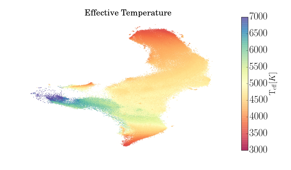
(a)

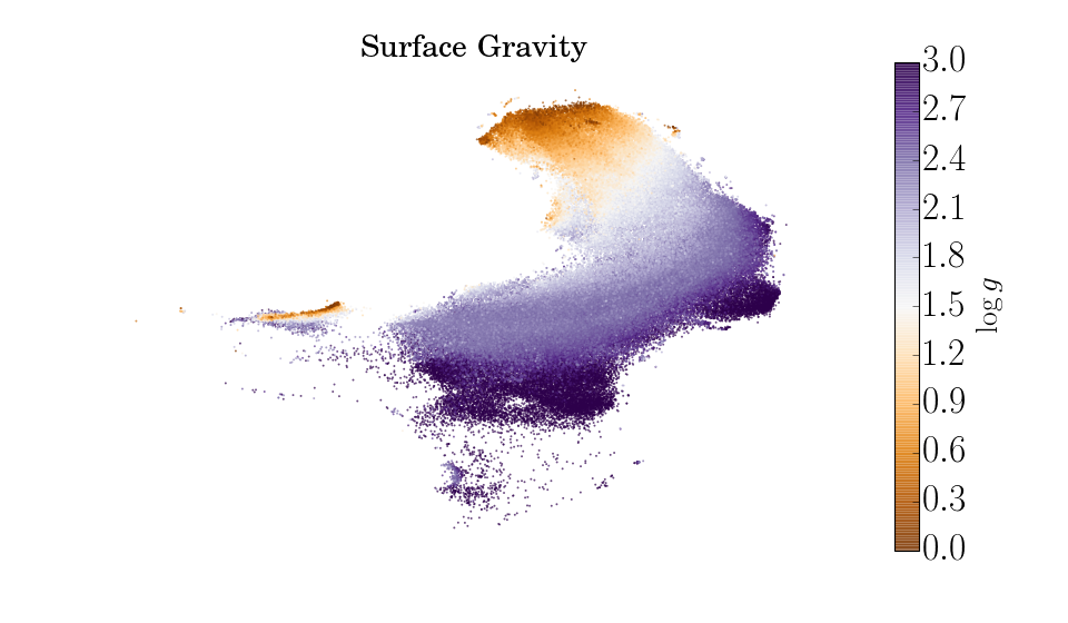
(b)

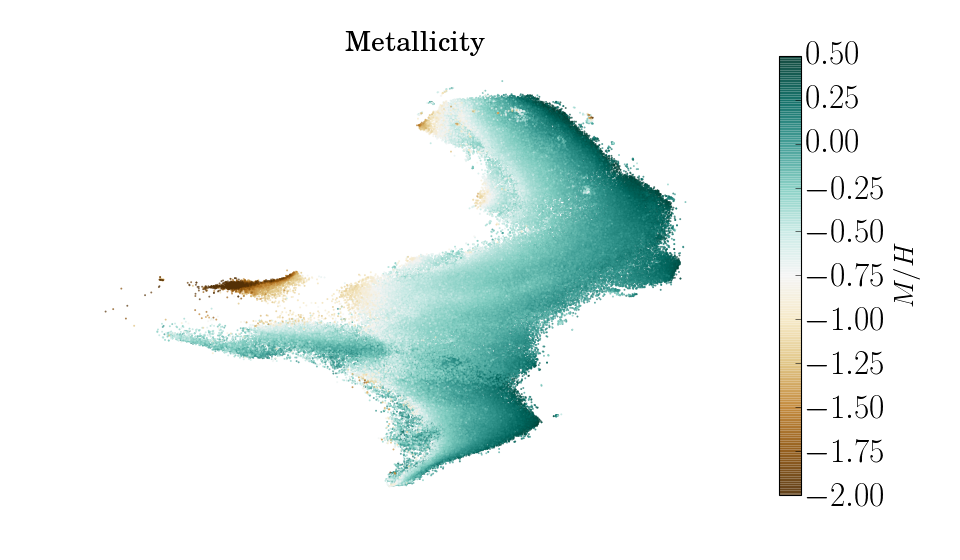
(c)

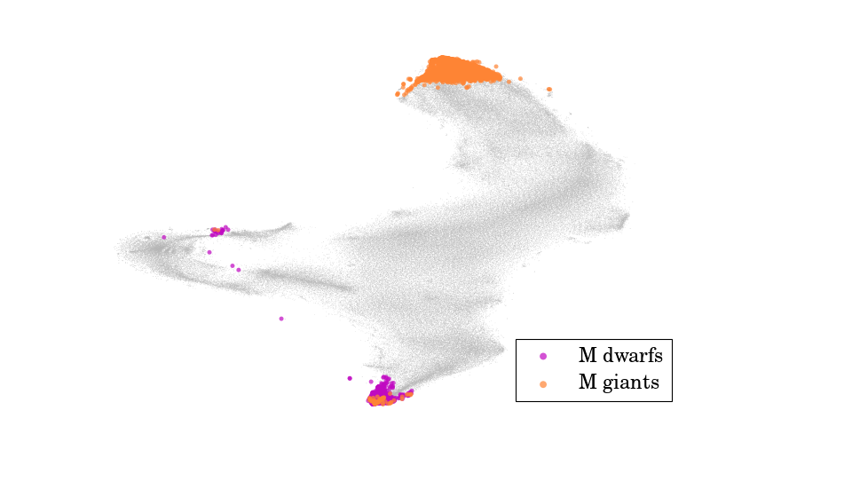
(d)

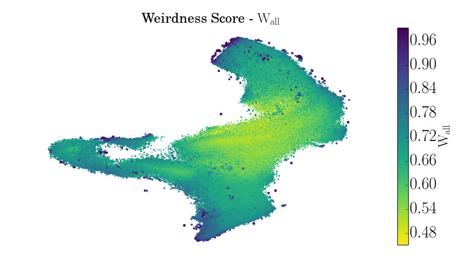
(e)

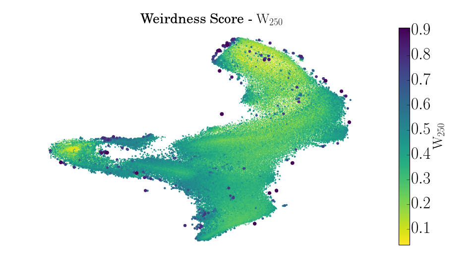
(f)

Figure 1: t-SNE map of our distance matrix. Each point on the map represents a star, where spectrally similar objects cluster on small scales. The axes do not have any physical significance. In the different panels, different coloring schemes are presented. Panel (a): effective temperature, panel (b): surface gravity, panel (c): metallicity, panel (d): highlighted M-type stars. The values used for the different coloring are taken from ASPCAP. Stars with no available value for a parameter do not appear on the map. For example, many dwarf stars do not have $\log{g}$ values, so the clusters containing dwarfs disappear from the $\log{g}$ map. The complex structure of the sample is apparent. In panels (e) and (f) we color the map by the weirdness score. $W_{all}$ is in panel (e), and $W_{250}$ is in panel (f). We see that when using $W_{250}$, low $\mathrm{T}_{\mathrm{eff}}$ stars no longer dominate the high weirdness score population, and we get a more diverse outlier population that is spread on the t-SNE map.

In panel 1d we see that some M-type stars are located far from the rest. We manually inspect these objects as an example to see if this is due to the algorithm mis-locating a few objects, or if these objects are really different from the rest of their respective groups. We find that in this case the objects really have different looking spectra, with poor ASPCAP fitting. For example, some of these misplaced-M-type stars turn out to be B-type emission line stars (Be stars).

From the t-SNE maps we learn that our distance matrix is capable of aggregating non-trivial information about the objects in the sample. Figure 1 shows that the distance matrix holds information about various physical properties, namely the figure is showing sequences in the effective temperature, surface gravity, and metallicity. These properties, in addition to the chemical abundances, affect the spectral features in non-trivial and partly degenerate ways, which we see are captured in the distance matrix.

The APOGEE pipeline derives the stellar parameters by means of best fitting templates. We see that some of the stars in the sample do not have derived parameter values. This is usually because these stars are extreme, at least with respect to the rest of the sample, and their stellar parameters fall outside the grid of spectral templates used by the pipeline. One can use the distance matrix to find these objects. As seen on the t-SNE map, the algorithm places the extreme objects next to the less extreme ones in a continuous sequence. In this sense we say that the similarity measure could be viewed as a generative model of the data.

Seeing here that globally the distance matrix captures the structure of the dataset, in the next two subsections we see that it could also be used to investigate the dataset at a ’smaller scale’ - by looking at the most similar objects.

3.4 Object retrieval

We can use the distance matrix to query the dataset for similar objects based on their spectra alone. We use the example of carbon rich stars to show that the algorithm can find objects that were not possible to find using their ASPCAP fit parameters. Carbon-rich stars have atmospheres with over-abundance of carbon compared to oxygen. In this case the excess carbon (i.e., carbon that is not tied in $\mathrm{CO}$) will allow $\mathrm{CN}$ (and other carbon molecules) to form. In regular stars there will be excess oxygen, that will form $\mathrm{OH}$. In Figure 2 we show a t-SNE map colored by the carbon to oxygen abundance ratio, from ASPCAP.

Focusing on a cluster of carbon rich stars we see that the objects are sequenced on the map according the the C/O abundance ratio. Most importantly we see that a number of objects without pipeline abundance value are located at the top of the sequence. We suggest that the pipeline is not able to fit these objects due to them having extreme abundances, and due to the difficulty of abundance analysis of spectra with very strong molecular lines. We manually inspect the 51 objects with no ASPCAP value shown in Figure 2 and see that they all show strong $\mathrm{CN}$ and weak $\mathrm{OH}$, typical for carbon rich stars. Moreover, all of the 35 objects that have SIMBAD (Wenger et al., 2000) entry are classified as carbon stars, making the 15 objects without SIMBAD entry carbon star candidates. We note that many of these objects were observed as part of the APOGEE-2 AGB stars ancillary program, see Zasowski et al. (2017).

This in an example of a query for objects based on their spectra, instead of on their fit parameters. This is of importance for objects with bad or nonexistent fit parameters, that would otherwise be lost in the dataset. In a large enough dataset it is very likely such objects will exist, these can be extreme cases of known phenomenon outside the range of the model, rare objects outside the scope of the model, or other types of outliers in the dataset.

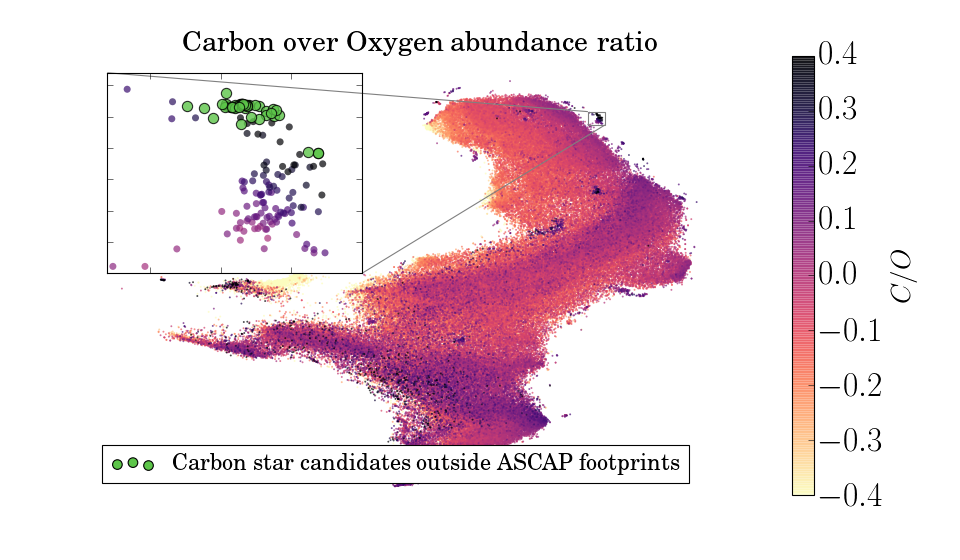
Figure 2: A t-SNE map colored by the carbon to oxygen abundance ratio, from ASPCAP. We focus on a cluster of carbon rich stars. We see that, according to a sequence visibly detectable on the map, objects at the high end of the sequence are not fitted by ASPCAP. Detecting these objects is possible using the similarity matrix.

3.5 Spectroscopic twins

The distance matrix produced by the algorithm can be used for finding objects with spectra similar to each other, objects sometimes referred to as spectroscopic twins. This is trivially achieved by sorting the distance matrix.

One use of spectroscopic twins is measuring distances (Jofré et al., 2015). Twin stars will have the same luminosity, and if we know the distance to one of the stars (e.g. using parallax), we can calculate the distance to the other by comparing observed magnitudes. Jofré et al. (2015) looked for spectroscopic twins among 536 FGK stars, and detected 175 pairs with spectra indistinguishable within the errors. As we work with a rather homogeneous sample of $\sim 10^{5}$ stars, we expect a large fraction of (multiple) twins.

Example spectra for spectroscopic twins are shown in 8b. It can be seen that the pairs have virtually identical spectra. Note that in the top example in Figure 8b one of the spectra lacks an ASPCAP fit, preventing identification of a twin via these parameters. The middle pair have very similar parameters, while the bottom twins show more significantly different parameters. Our method finds them all, irrespectively.

One thing we note is that this method for finding twins works well for the common object types (common in terms of representation in the dataset), but might be less so for underrepresented types of objects (in which case we still get similar spectra, but not identical). The reason being that our unsupervised RF uses more extensively the features that are important for regular objects, and as a result it can separate objects based on subtle differences in these features. For other features that might not be important to most of the objects (for example hydrogen absorption or emission), the RF uses cruder cuts to separate objects.

As a test for the selection of twin objects we look at the angular separation of stars with similar spectra. APOGEE stars living in the same environment are more likely to have similar physical properties, and thus similar spectra. We expect that pairs of stars we detect as having similar spectra will have higher probability to be located near each other compared with random pairs of stars. We note that there is an observational effect playing a role here - the APOGEE sample is not uniform in different parts of the galaxy (for example, dwarfs from the galactic bulge are too faint for APOGEE and are not observed). In Figure 3 we show the distribution of the angular separation of each star in our sample with its nearest neighbor (as defined by our distance matrix), compared to random pairs of stars. Clearly the twins we find are physically associated. We release our entire distance matrix, and we will update it with future data releases, allowing others to use the twins for further study. We note that our methodology does not allow one to compare well objects with different $S/N$, nor does it give a statistically meaningful similarity measure. However, it bypasses the difficulties of comparing spectra in data or model space, while producing very robust results. An additional example for using a distance metric to find similar objects is found in Jofré et al. (2017), who looked for nearest neighbors on a t-SNE map of RAVE stars in search for spectroscopic twins. To build the t-SNE map euclidian distance were used.

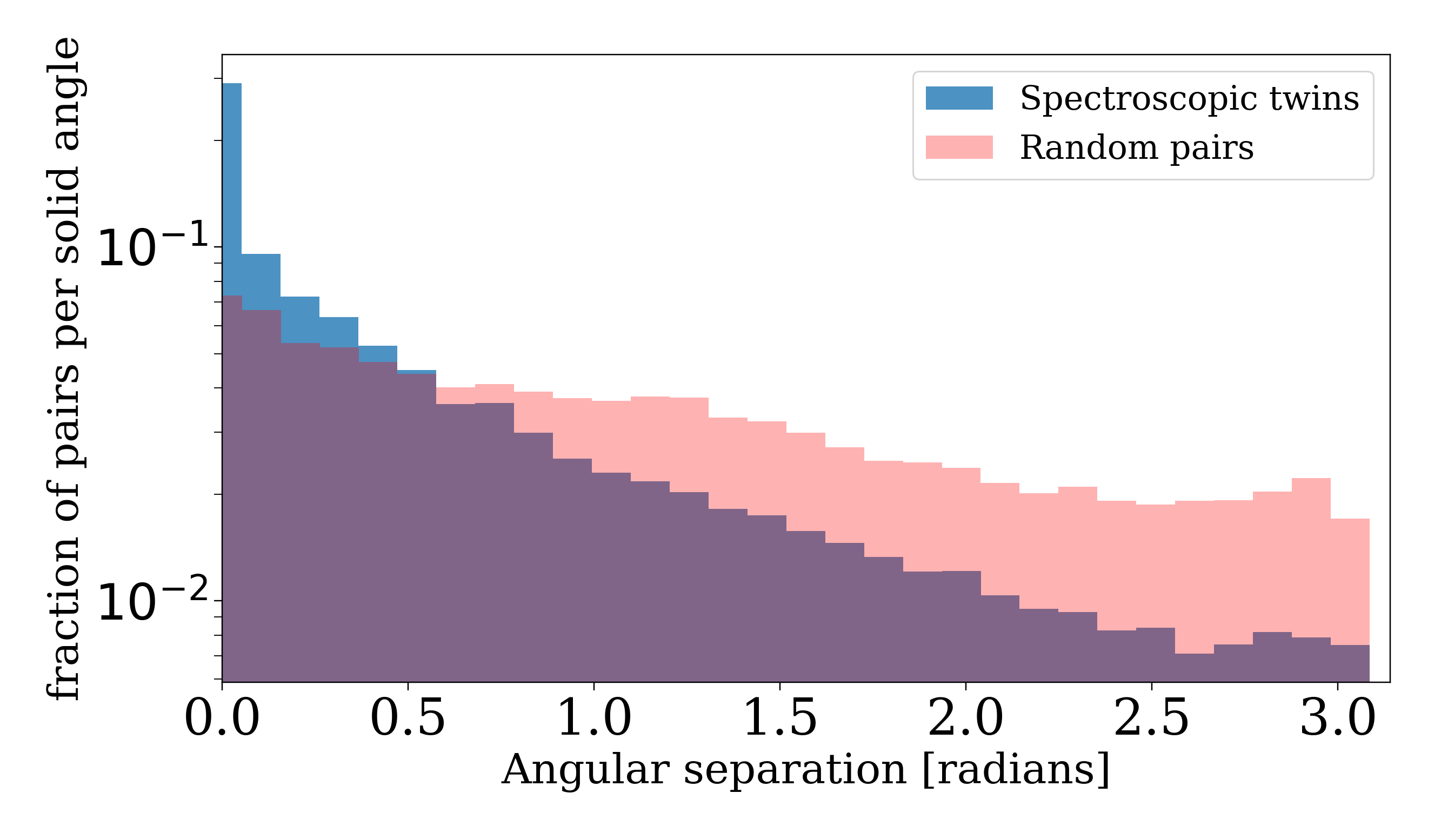
Figure 3: A comparison between angular separation of pairs of stars detected as having similar spectra, and random pairs of stars. The similar spectra stars shown here are each star in our sample and its nearest neighbor according to our distance matrix.

4 Efficient outlier detection

An important usage of the distance matrix is outlier detection. For this purpose we calculate a weirdness score for each object in the sample. This weirdness score is calculated by summing over the distance matrix. In this section we use the t-SNE visualization in order to understand the properties of this weirdness score. We present a new, local, definition of a weirdness score. We use this local weirdness score for APOGEE stars, and find it is more suitable for detecting outliers.

We can use the t-SNE map in order learn about the weirdness score properties. In Figure 1e we color the t-SNE map by the weirdness score. The central, low $\mathrm{W_{all}}$ part of the t-SNE map contains about half of the objects in the sample. These objects are $\mathrm{G}$ and $\mathrm{K}$ giant stars, with weak molecular features in their spectra, but with prominent metallic features. They comprise one large group of objects with similar spectra. Below we refer to these objects as the main group. Example spectra for such objects are presented in Figure 8a. For each object in the figure we present the percentile of the object’s weirdness score, i.e. the percent of the objects with lower weirdness score.

In order to better understand the properties of $W_{all}$, we examine its distribution in Figure 4. The distribution decreases smoothly to high weirdness except for two bumps. We interpret the bumps as clusters of stars in our similarity space. One bump consists partially of low-temperature stars, and the other is due to stars with weak or non existent absorption lines - - metal poor stars and telluric calibration targets. The bumps in the distribution of $W_{all}$ are due to the fact that there is one dominant cluster of objects in the dataset, and the objects in smaller clusters receive a weirdness score based on how different they are from objects in the main cluster. These results might be useful to detect clusters, or to clean up the dataset from objects outside the main group, but in order to find small classes of interesting outliers, we need a better outlier definition.

Figure 4: $W_{all}$ distribution for all objects in the sample. The two bumps in the distribution are composed mostly of objects with no ASPCAP fit parameters. Inspecting the spectra of these objects, we see that one bump contains low $\mathrm{T}_{\mathrm{eff}}$ stars, while the other contains low metallicity and hot telluric calibration stars (i.e. stars with weak or non existent absorption lines).

To address the issue described above we introduce the ’nearest neighbors weirdness score’, a modification to the algorithm that produces ’better outliers’ for the APOGEE dataset. When looking for better outliers, we wish to get several different types of objects detected as outliers, in contrast to a weirdness score that strongly correlates to a single attribute (e.g. the effective temperature). In addition we expect to be able to detect known outliers such as binaries and bad spectra.

Instead of defining outliers based on their average distance to the entire sample, we use a more local measure, and for every object we calculate distances to its nearest neighbors. This measure of unusualness is used for distance-based outlier detection in other fields (Knorr & Ng, 1999; Knorr et al., 2000). The resulting weirdness score distribution is shown in figure 5. We can see that the bumps in the weirdness score distribution go away for a small enough number of nearest neighbors. When choosing the number of nearest neighbors to use in the weirdness score calculation, one can check at what point the weirdness score distribution does not contain bumps.

Figure 5: Weirdness score distribution for different numbers of nearest neighbors included in the calculation.

A t-SNE map with the 250 nearest neighbors weirdness score ($W_{250}$) is shown in Figure 1f . Clearly, there is a group of stars that have persistently high (percentile) weirdness score for any number of nearest neighbors used. On the other hand, the high $\mathrm{T}_{\mathrm{eff}}$ stars no longer have high weirdness score for small numbers of nearest neighbors. This results in various other groups of stars receiving higher percentile weirdness score.

An open question regarding many outlier detection algorithms is setting a threshold on the weirdness score, i.e., determining above which weirdness score we mark an object as an "outlier" and inspect it further. The t-SNE map could be of help here too: looking at the $W_{250}$ t-SNE map (Figure 1f) we can see that for each group of stars on the map, the edges receive higher weirdness score. We do not want to mark these edges as outliers, and from the t-SNE map we determine that this would be achieved with a threshold of 0.6, for this specific dataset.

The classification of the outliers is made easier by sorting the objects using their position on the t-SNE map. This way we can classify groups of similar objects instead of one object at a time. Another method we try for outlier inspection is called DEMUD (Wagstaff et al., 2013). Instead of examining the outliers sequentially, one starts from the weirdest object, and then inspects the weird object that is the farthest from the first, followed by the one farthest from the first two, and so forth. The idea is to sample the different populations of outliers quickly, stopping once we start seeing the same types of objects repeating. For the final classification of the outliers we chose a threshold on the weirdness score (as discussed above) and use the t-SNE map to help with the classification. This is followed by taking a lower threshold on the weirdness score and using DEMUD to look for additional types of outliers. This second step did not result in new types of outliers.

5 APOGEE Outliers

In this section we present the results of manual classification of the highest $W_{250}$ stars. Here we use results from both DR14 and DR13, as in DR14 many objects have poorly determined continua. In total we look at 577 objects. The distribution of the different groups of outliers for DR13 only is shown in Figure 6. We find the following large groups: Be stars, young stellar objects, carbon enriched stars, double lined spectroscopic binaries (SB2), fast rotators, M dwarfs, M giants and cool K giants (these stars have the highest $W_{all}$), and stars with bad spectra. In addition we find a number of objects that do not fit into any of the above classes.

“Bad spectra” are objects with ASPCAP warn flags, combined with a strange looking spectrum. The flags we encounter for the outliers are commissioning, persist high, and persist jump neg(high). Other "bad spectra" objects are not flagged but have faulty spectra. These appear only in DR14 and we discuss them below.

We note that these classes are not mutually exclusive (in Figure 6 each object is assigned to a single class we believe describes it best).

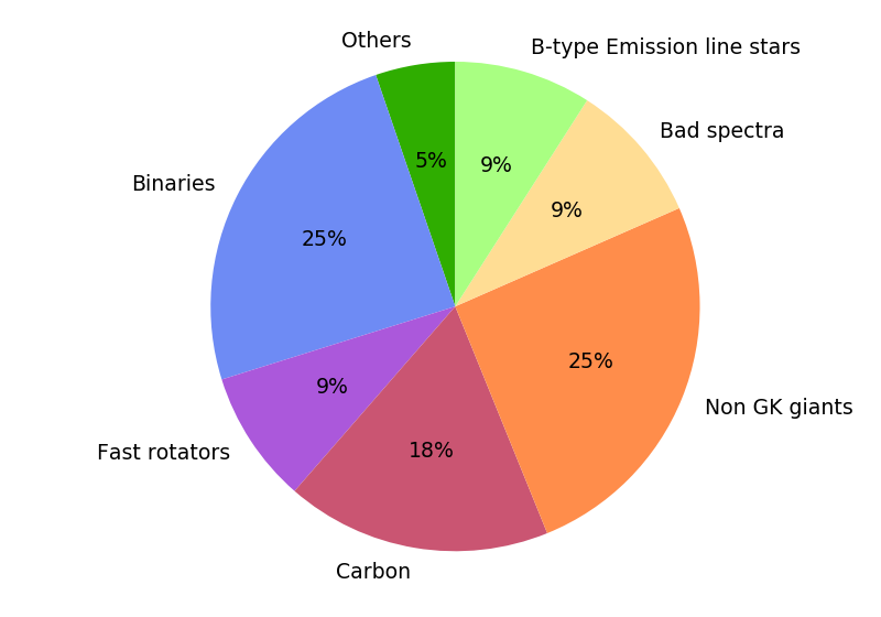
Figure 6: Results of the manual classification of 348 highest $W_{250}$. In the next sections we discuss each of these groups. The Non GK giants group contains mostly M dwarfs. This figure refers to DR13.

5.1 B-type emission line stars

The objects in this group are Be stars. APOGEE targeted approximately 50 known Be stars in an ancillary program, while the additional Be stars in the APOGEE sample were originally targeted as telluric standard stars. Chojnowski et al. (2015a, 2017) compiled a catalog of 238 Be stars in the APOGEE dataset. They identified these stars by visual inspection.

We find 40 Be stars not included in the Chojnowski et al. (2015a) catalog. These new Be stars first appeared in DR14. For 26 of these stars emission was never reported before. We list these objects in table 2. Some of these stars were detected as outliers, while the rest were found by inspecting the neighbors, in the distance matrix and t-SNE map, of the outliers.

As seen in Figure 8j, these stars have double peaked H-Br emission lines and weak absorption lines. For some Be stars, metallic emission is also present. ASPCAP fails to derive radial velocities for these objects, due to their unusual spectra.

5.2 Spectroscopic binaries

Example spectra of SB2s are shown in Figure 8c along with their best fitting synthetic spectra. As seen, ASPCAP does not account for binarity. For some of the SB2s ASPCAP fits broad lines, and for others it fits only one of the two sets of lines. In general the APOGEE reduction pipeline does not have an automatic binary identification routine (Nidever et al., 2015).

Chojnowski et al. (2015b) compiled a catalog of spectroscopic binaries in APOGEE . The catalog is constructed by searching for multiple peaks in the spectra cross correlation function, when comparing to the synthetic template spectra. 15 of the 72 binaries we find as outliers are not listed in the catalog of Chojnowski et al. (2015b) and are therefore new.

5.3 Fast rotators

Broad line stars are also detected as outliers. ASPCAP fits broad lines well for dwarf stars but not for giants, as can be seen in Figure 8d. These stars are all flagged with suspect broad lines by the ASPCAP pipeline.

5.4 Carbon rich stars

Carbon rich stars (discussed in section 3.4) are also detected as outliers. In Figure 8e we can see the strong $\mathrm{CN}$ compared to $\mathrm{OH}$ lines for a few carbon enriched stars. The weirdness score increases with the strength of the $\mathrm{CN}$ features.

5.5 Young stellar objects

Stars in this group show both H-Br emission lines as well as regular metallic absorption lines. They are mostly young stars included in the INfrared Survey of Young Nebulous Clusters (IN-SYNC, Cottaar et al., 2014). We detect stars with both broad and narrow emission, and with absorption that can be broad or narrow as well as double lined (SB2s). SIMBAD classification for stars in this group include ’Variable star of Orion type’, ’T Tau-type Star’, ’Pre-main sequence Star’, and ’Young stellar object’.

5.6 M dwarfs

M dwarf stars are also detected as outliers. This is due to the small number of M dwarf stars in the APOGEE sample. Example spectra are in Figure 8g.

5.7 Other outliers

Some of the objects detected as outliers did not fall into any of the above classes. These include a brown dwarf, a Wolf-Rayet star, a few AGB stars including an OH-IR star, and known variable stars, as well as three red supergiants observed in the massive stars ancillary program. Also detected as outliers are special non stellar targets, such as the center of M32, a few M31 globular clusters, and three planetary nebulae.

Two outliers show double peaked H-Br emission lines, as well as absorption lines typical to the APOGEE dataset. Both of these objects show RV modulations, suggesting they are multiple star systems. For the first, 2M04052624+5304494, the RV modulation of the absorption lines (determined from APOGEE visit spectra), could be modeled with a period of $\mathrm{P}=11.152\pm 0.072\;\mathrm{days}$, and amplitude of $\mathrm{K}=78\pm 15\;\mathrm{km}\;\mathrm{s}^{-1}$. The emission lines in the APOGEE spectra show smaller RV modulation, if any. For the second, 2M06415063-0130177, the absorption lines RV changes by $\sim 160\;\mathrm{km}\;\mathrm{s}^{-1}$ between two APOGEE visits. The visits are separated by 28 days. For the emission lines we could not get a good estimate on the RVs, as the emission line profiles change significantly between the visits. A CoRoT light-curve is available for this system, showing clear periodic modulation. A period of $\mathrm{P}=29.04\;\mathrm{days}$ was derived for this light-curve by Affer et al. (2012). We note that this period does not agree with the RV modulation. For both of these systems additional work is required to determine their nature.

We also detect a group of objects with similar, very broad features. Most of these objects have SIMBAD classifications as contact binaries, mainly W Ursae Majoris.

A few objects remain unexplained. We divide these objects into two groups. In the first group we have objects with spectra that seems to have similar features to typical APOGEE red giants (by means of visual inspection). The second group contains stars with spectra that are clearly different from typical APOGEE red giants. We refer to the first group as unexplained red giants, and to the second group as unexplained non red giants. Some of the unexplained red giants stars have low carbon and high nitrogen ASPCAP abundances. Inspecting their spectra, we do see significantly weaker CO features relative to low weirdness score stars with similar stellar parameters. One of these stars, 2M17534571-2949362, is discussed in Fernández-Trincado et al. (2017) as having low Mg, but high Al and N abundances. There are three unexplained non red giants, the first is 2M03411288+2453344, which was targeted as a telluric calibrator target. As could be seen in Figure 8h, the ASPCAP fit does not catch many of the features in the spectrum, in particular there is no H-Br absorption. The cross correlation function shows a single peak, suggesting it is not a binary star. There are 3 visits to this star, all showing the same features. The objects most similar to this one, according to the distance matrix, do not show similar features. 2M05264478+1049152 has very broad features that we do not identify. Same goes for 2M23375653+8534449 which also has a single emission line centered at $\lambda=16055[\mbox{\AA}]$ that we cannot identify. We show the spectra of the unexplained non red giants in Figure 7.

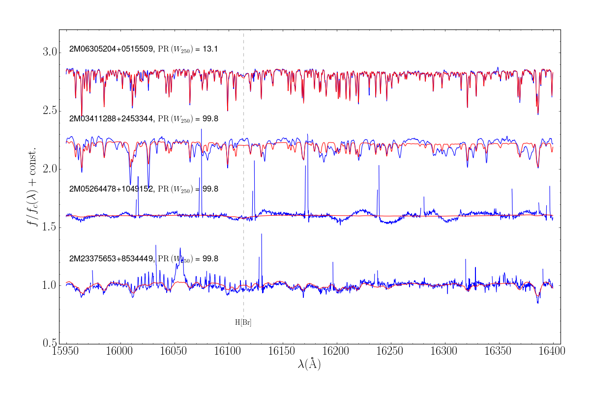
Figure 7: Spectra for the three unclassified outliers. Top spectrum is a typical APOGEE red giant, for comparison. The red line is the ASPCAP fit and the blue line is the PCN spectrum, except where indicated. $\mathrm{PR}\left(W_{250}\right)$ indicates the percentile of objects with lower weirdness score. Relative fluxes are offset by a constant for display purposes.

5.8 Bad reductions

In DR14 roughly half of the high weirdness score objects have badly determined continua. We show a few examples in Figure 8. These objects can be divided into two groups. For the first group, the issue seems to be a bug in the ASPCAP PCN process. For objects in this group the combined unnormalized spectra looks regular, as well as the DR13 PCN spectra (for objects with available DR13 data). For the second group already at least one of the visit spectra is faulty, and this error propagates down the pipeline. Examples for both of these errors are presented in Figure 8i.

6 Summary

In this work we calculate a similarity measure for APOGEE infrared spectra of stars. We show that this similarity matrix traces physical properties such as effective temperature, metallicity and surface gravity. Such a similarity matrix could be used for object retrieval, i.e., finding objects that are similar to a given example, it can be used to detect outliers, and more generally to assist learning about the structure of a dataset. The similarity is obtained without inputing information derived by model fitting, and thus the similarity could be used to query and learn about objects that are not well fitted by the pipeline and as such are hard to find using the fit parameters database.

As noted above, we find that the unsupervised RF is capable of aggregating complex spectral information into a single number, the pair-wise distance between two objects. We find that various stellar parameters are encoded into this distance, and that the resulting RF represents a general model of stellar spectra (Baron & Poznanski (2017) showed that this is true for spectra of galaxies). As such, one can imagine inverting the process, and using the trained RF to generate “real-looking" objects, which is in turn a generative model.

Using this unsupervised RF distance matrix and dimensionality reduction techniques, one can study the structure of the data, and the relations between different classes of objects within a dataset. However, it is worth noting that much of the insight gained about the APOGEE sample was made possible using the derived ASPCAP stellar parameters. Without these labels, coloring the t-SNE map would not have been possible. While our proposed unsupervised distance matrix contains various types of information, the extraction of this information still heavily depends on annotations of the distance matrix. Thus, for many applications, it is only the combination of our approach and existing knowledge about the dataset that can be useful to gain additional insight.

Using our distance matrix to detect outliers, we find objects from the following types of known classes: B-type emission-line stars, carbon rich stars, spectroscopic binaries, broad line stars, young stars, bad spectra, and M dwarfs (which are ordinary but underrepresented in the dataset), showing that the algorithm is capable of detecting a wide variety of phenomena. A few dozens of objects that were detected as outliers did not fall into any of the large groups, these include special targets such as galaxies, globular clusters, and planetary nebulae, stars with unusual abundances, contact binaries, stars observed with the massive star ancillary program and more. Three outliers remain without explanation.

Some of the carbon rich outliers have a poor ASPCAP fit, though these groups are included in the ASPCAP stellar spectral library. Possibly the objects without a good fit are extreme cases and could be used to improve and test the pipeline. The SB2s detected as outliers have diverse types of spectra and could be used to test SB2 detection specific algorithms. Bad spectra objects and underrepresented objects are not interesting by themselves, but detecting them could be useful in order to clean the sample and find bugs in the pipeline. Finding new Be stars is an example for detection of new objects of known types using the distance matrix or t-SNE map. This is especially useful in larger surveys, where visual inspection is not feasible.

The use of t-SNE to visualize the distance matrix was also useful for the purpose of outlier detection. This enabled us to speed up the classification of the outliers by classifying nearby objects together. More importantly, the t-SNE map proved to be useful in learning about the regular objects in the data set, an important step to take before looking at the outliers. Viewing spectra of objects located in different regions of the t-SNE map allowed us to quickly review the different classes of regular objects. For the APOGEE dataset, in which there is one large group of similar objects, a nearest neighbors weirdness score, or a ’local’ weirdness score, was needed in order to detect the interesting outliers. Although this was not required to detect the interesting outlying galaxies in Baron & Poznanski (2017), we believe the the local weirdness score is more general and should be used in future work. The number of nearest neighbors to use when calculating the local weirdness score is dataset dependent. Coloring the t-SNE map by the different weirdness scores or building t-SNE maps with different perplexities, can help decide on which number of nearest neighbors is appropriate. It is also possible that in order to detect all interesting objects one type of nearest neighbors weirdness score would not be enough, as different types of outliers can come in different (small) cluster sizes. In our case the outliers population seemed robust to a number of nearest neighbors from a few to a few thousands. We note that for the map shown in Figure 1 we used perplexity of 2000. This value was chosen in order to make the visualization relatively simple. With smaller perplexity we obtained maps with more complex small scale structure, such as small clusters. These maps could be useful for investigating the data further but for a clean visualization of the large scale structure we used a high perplexity map.

Future work could involve combining the distance matrix, which is based on spectral data alone, with other types of available data. A natural direction is the physical position of a star. For example, one can look for stars that are normal compared to the entire population of stars, but are weird when compared to their local environment. A table with the 100 nearest neighbors of each object, including their respective distances, is available online. We also include the coordinates for the t-SNE map shown above. Examples for using these data products are available in a Jupyter Notebook .

Appendix A Spectra and tables

In Figure 8 we show example spectra of objects from the different outlying groups, as well as spectroscopic twins.

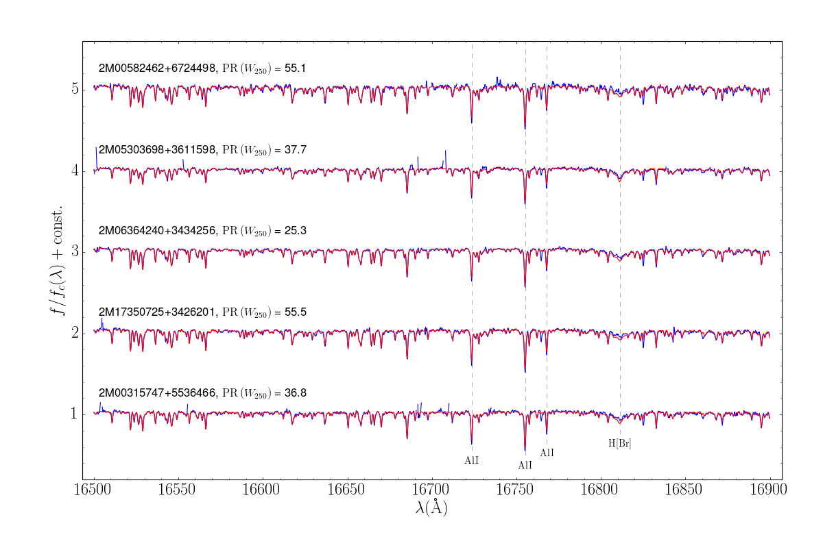
(a) Regular objects, i.e. objects with low weirdness scores. Clearly, all have similar spectra. $\mathrm{PR}\left(W_{250}\right)$ indicates the percentile of objects with lower weirdness score.

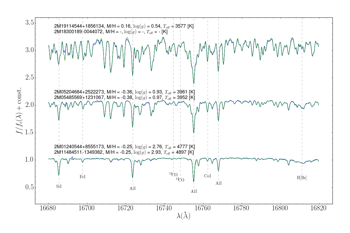
(b) Three example pairs of spectroscopic twins. The twin spectra are over-plotted, one in green and the other in blue. Note that in the top example one of the stars lacks an ASPCAP fit, preventing identification as a twin via these parameters.

Figure 8: Example spectra for different groups of objects. The spectra plots were made using the APOGEE toolkit by Bovy (2016). The red line is the ASPCAP fit and the blue line is the PCN spectrum, except where indicated. $\mathrm{PR}\left(W_{250}\right)$ indicates the percentile of objects with lower weirdness score. Relative fluxes are offset by a constant for display purposes. In every panel we choose the most informative wavelength range.

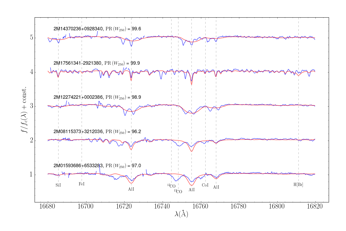
(c) Spectroscopic binaries.

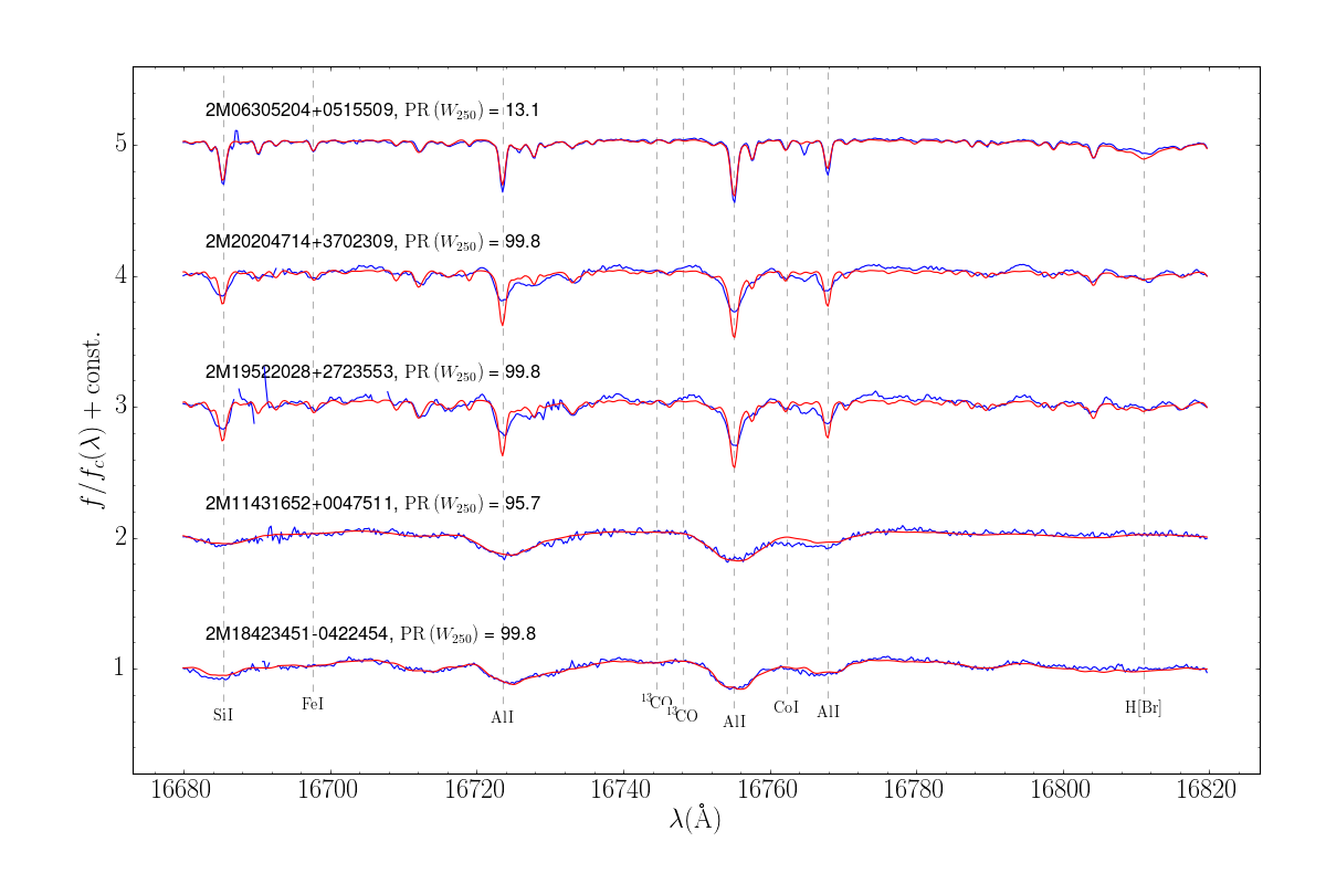
(d) Fast rotators. Top spectrum is a typical APOGEE red giant, for comparison.

Figure 8: Continued.

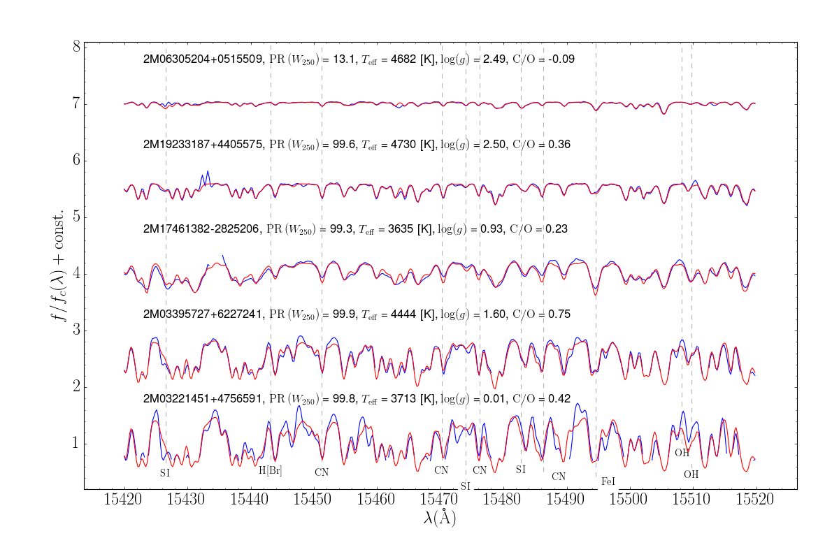
(e) Carbon enriched stars. Top spectrum is a typical APOGEE red giant, for comparison.

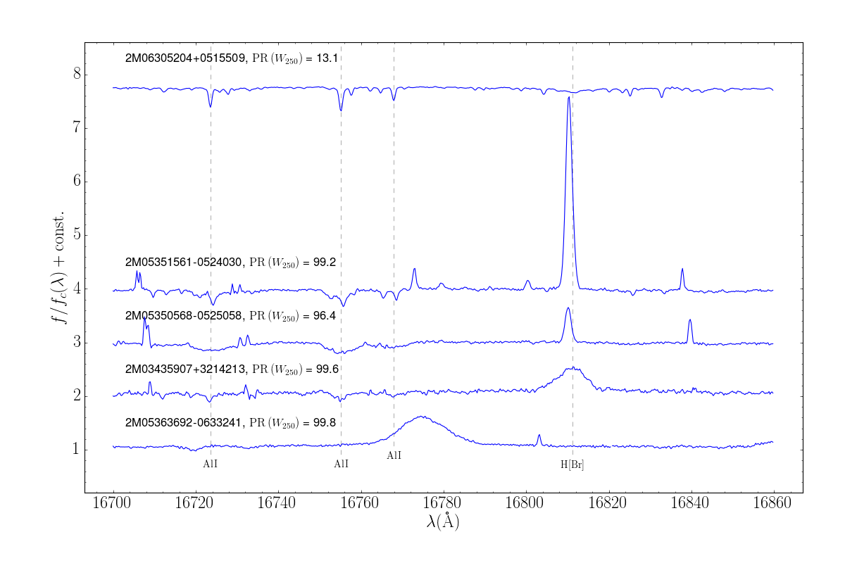
(f) Stars with both absorption and hydrogen emission. Top spectrum is a typical APOGEE red giant, for comparison. We see both narrow and broad emission stars, and also both narrow and broad absorption. The second spectra from the top is also an SB2. The bottom spectrum has bad RV determination.

Figure 8: Continued.

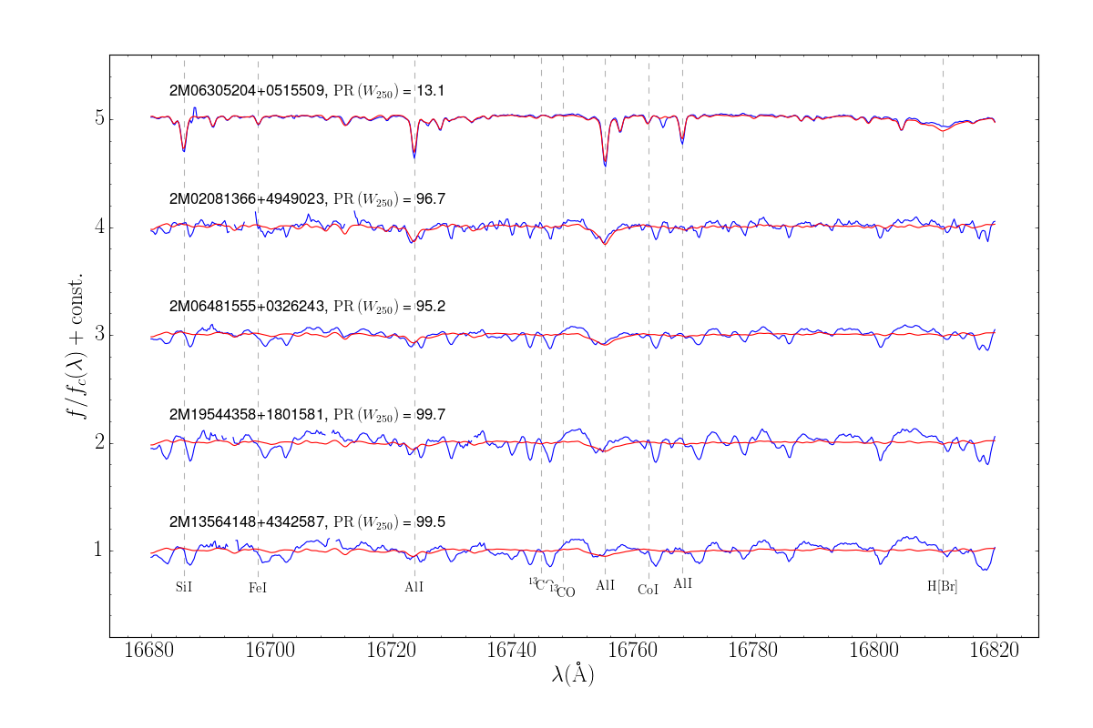
(g) M dwarfs. Top spectrum is a typical APOGEE red giant, for comparison. M dwarfs are detected as outliers due to their underrepresentation in the APOGEE dataset.

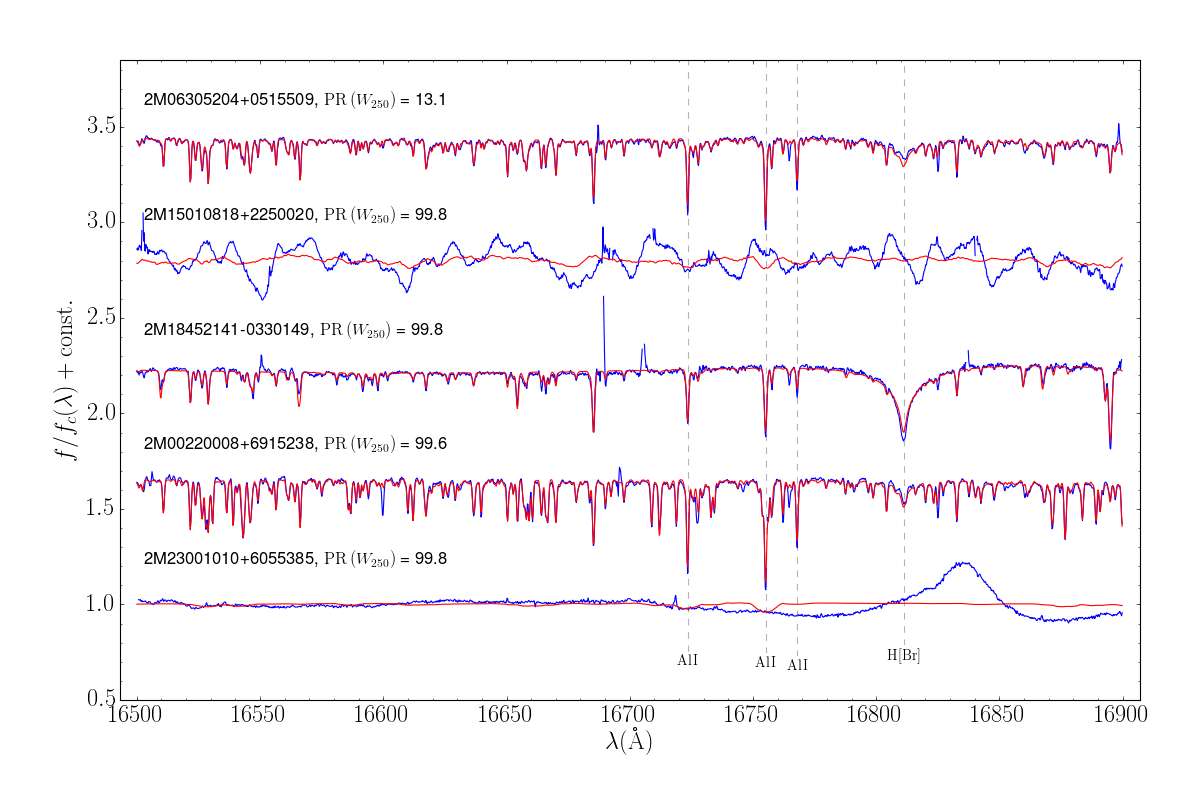
(h) Stars from the ’others’ pile. Top spectrum is a typical APOGEE red giant, for comparison. Starting from the second from top, the four outlying spectra are brown dwarf, massive star target, unexplained red giant, and a Wolf-Rayet star.

Figure 8: Continued.

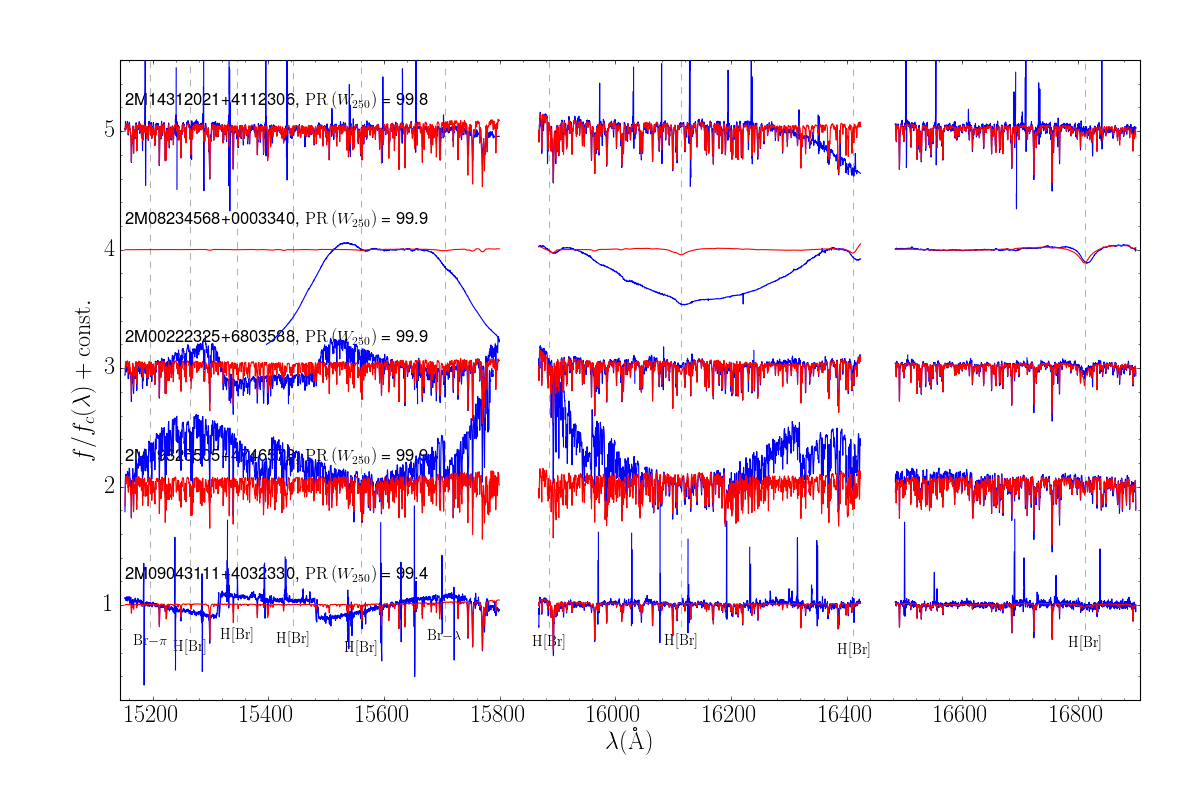
(i) DR14 Faulty spectra. For the top two objects the problems are due to an issue in the PCN process, for the bottom three one of the visit spectra is bad.

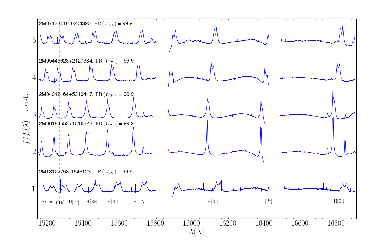
(j) B-type emission line stars showing double peaked hydrogen emission. The emission lines are not on the dotted lines due to wrong RV determination by the APOGEE pipeline.

Figure 8: Continued.

In Table 1 we present all the objects detected as outliers, and did not fall into any of the large groups. Tables with the objects in the rest of the groups are available online.

APOGEE ID	RA [deg]	DEC [deg]	Classification
2M15010818+2250020	225.284	22.8339	Brown dwarf
2M14323054+5049406	218.127	50.828	Contact binary
2M03114116-0043477	47.9215	-0.72993	Contact binary
2M14304297+0905087	217.679	9.08575	Contact binary
2M13465180+2257140	206.716	22.9539	Contact binary
2M14120965+0508201	213.04	5.13893	Contact binary
2M16145863+3016356	243.744	30.2766	Contact binary
2M03242324-0042148	51.0969	-0.704119	Contact binary
2M03242324-0042148	51.0969	-0.704119	Contact binary
2M16241043+4555265	246.043	45.924	Contact binary
2M16524137+4723275	253.172	47.391	Contact binary
2M06415063-0130177	100.461	-1.50494	Double-peaked emission
2M04052624+5304494	61.3594	53.0804	Double-peaked emission
2M13145725+1713303	198.739	17.2251	Galaxy
AP00425080+4117074	10.7117	41.2854	Globular cluster
AP00442956+4121359	11.1232	41.36	Globular cluster
AP00430957+4121321	10.7899	41.3589	Globular cluster
AP00424183+4051550	10.6743	40.8653	Globular cluster
AP00424183+4051550	10.6743	40.8653	Globular cluster
AP00431764+4127450	10.8235	41.4625	Globular cluster
2M18445087-0325251	281.212	-3.42364	Massive star
2M18452141-0330149	281.339	-3.50416	Massive star
2M18440079-0353160	281.003	-3.88778	Massive star
2M03411288+2453344	55.3037	24.8929	Unexplained non red giant
2M05264478+1049152	81.6866	10.8209	Unexplained non red giant
2M23375653+8534449	354.486	85.5792	Unexplained non red giant
2M04255084+6007127	66.4619	60.1202	Planetary nebula
2M21021878+3641412	315.578	36.6948	Planetary nebula- Egg nebula
2M18211606-1301256	275.317	-13.0238	Planetary nebula- Red Square nebula
2M17534571-2949362	268.44	-29.8267	Unexplained red giant
2M06361326+0919120	99.0553	9.32001	Unexplained red giant
2M00220008+6915238	5.50037	69.2566	Unexplained red giant
2M21184119+4836167	319.672	48.6047	Unexplained red giant
2M20564714+5013372	314.196	50.227	Unexplained red giant
2M05501847-0010369	87.577	-0.176939	Unexplained red giant
2M23001010+6055385	345.042	60.9274	Wolf-Rayet star
2M05473667+0020060	86.9028	0.33501	Young stellar object

Table 1: Outliers that and did not fall into any of the large groups.

In Table 2 we list Be stars which are new in DR14 and thus not included in the Chojnowski et al. (2015a) catalog.

APOGEE ID	RA [deg]	DEC [deg]
2M20383016+2119439	309.626	21.3289
2M22425730+4443183	340.739	44.7218
2M06490825+0005220	102.284	0.089448
2M04480651+3359160	72.0271	33.9878
2M05284845+0209529	82.2019	2.16471
2M21582976+5429057	329.624	54.4849
2M22082542+5413262	332.106	54.2239
2M19322817-0454283	293.117	-4.90786
2M03145531+4841448	48.7305	48.6958
2M21523408+4713436	328.142	47.2288
2M04454937+4323302	71.4557	43.3917
2M18574904+1758251	284.454	17.9736
2M05312677+1101226	82.8616	11.0229
2M05384719-0235405	84.6967	-2.59459
2M22075623+5431064	331.984	54.5185
2M21380289+5037030	324.512	50.6175
2M06521036-0017440	103.043	-0.29556
2M04125427+6647203	63.2262	66.789
2M22142219+4206020	333.592	42.1006
2M04493134+3313091	72.3806	33.2192
2M02374876+5248458	39.4532	52.8127
2M05122466+4816538	78.1028	48.2816
2M23570808+6118272	359.284	61.3076
2M05441926+5241437	86.0803	52.6955
2M18042714-0958113	271.113	-9.96982
2M06514059+0019363	102.919	0.326773
2M02273460+4813548	36.8942	48.2319
2M23293672+4822513	352.403	48.3809
2M18040936-0827329	271.039	-8.45915
2M21151579+3235270	318.816	32.5909
2M06552851+2430188	103.869	24.5052
2M19575932+2714001	299.497	27.2334
2M04563331+6345566	74.1388	63.7657
2M19562230+2626258	299.093	26.4405
2M10214707+1532036	155.446	15.5344
2M05271779+1308569	81.8241	13.1492
2M02571539+4601118	44.3142	46.02
2M21504079+5518451	327.67	55.3125
2M04503901+3243187	72.6626	32.7219
2M22165865+6738450	334.244	67.6458

Table 2: Be stars.

In Table 3 we list carbon rich stars that were detected as outliers.

APOGEE ID	RA [deg]	DEC [deg]
2M21095891+1111013	317.495	11.1837
2M12553245+4328014	193.885	43.4671
2M08031240+5311340	120.802	53.1928
2M17552511-2517291	268.855	-25.2914
2M18442763-0614402	281.115	-6.24452
2M06211564-0124429	95.3152	-1.41194
2M12410240-0853066	190.26	-8.88517
2M13150364+1806426	198.765	18.1119
2M07384226+2131021	114.676	21.5173
2M05264861+2551545	81.7026	25.8652
2M16334467-1343201	248.436	-13.7223
2M13381781-1458456	204.574	-14.9793
2M13122536+1313575	198.106	13.2327
2M15000319+2955500	225.013	29.9306
2M21330683+1209406	323.278	12.1613
2M18455347-0328585	281.473	-3.48293
2M18495015-0235162	282.459	-2.58786
2M19425134+2235573	295.714	22.5993
2M19474632+2349074	296.943	23.8187
2M00242588+6221034	6.10785	62.3509
2M04501927+3947587	72.5803	39.7996
2M05012902+4023388	75.3709	40.3941
2M21053099+2952201	316.379	29.8723
2M01403590+6254392	25.1496	62.9109
2M04405098+4705190	70.2124	47.0886
2M18191371-1218145	274.807	-12.304
2M18030503-2157460	270.771	-21.9628
2M18015024-2638220	270.459	-26.6395
2M17520031-2308488	268.001	-23.1469
2M18052874-2505351	271.37	-25.0931
2M18063056-2435442	271.627	-24.5956
2M18111704-2352577	272.821	-23.8827
2M18115753-1503100	272.99	-15.0528
2M18185547-1119080	274.731	-11.3189
2M18524968-2834454	283.207	-28.5793
2M17301939-2913292	262.581	-29.2248
2M19295061+0010102	292.461	0.16951
2M19411240+4936344	295.302	49.6096
2M19003459+4408290	285.144	44.1414
2M19023427+4246148	285.643	42.7708
2M19095794+4325272	287.491	43.4242
2M06343313+0643006	98.6381	6.71686
2M01471583+5753060	26.816	57.885

Table 3: Carbon rich stars.

APOGEE ID	RA [deg]	DEC [deg]
2M21473632+5932259	326.901	59.5405
2M21544864+5916346	328.703	59.2763
2M11475977-0019182	176.999	-0.32173
2M18284700-1010553	277.196	-10.182
2M17043371-2212322	256.14	-22.209
2M19233187+4405575	290.883	44.0993
2M12553245+4328014	193.885	43.4671
2M14561660+1702441	224.069	17.0456
2M15015733+2713595	225.489	27.2332
2M15100330+3054073	227.514	30.902
2M23290070+5711558	352.253	57.1989
2M02403149+5600473	40.1312	56.0132
2M07094794+0006382	107.45	0.11062
2M07232483-0823577	110.853	-8.39936
2M03463234+3221127	56.6348	32.3536
2M19531095+4635518	298.296	46.5977
2M19200927+1317078	290.039	13.2855
2M21315424+5219122	322.976	52.3201
2M00334926+6837330	8.45529	68.6258
2M04174731+4211335	64.4472	42.1926
2M04195310+4109094	64.9713	41.1526
2M06372981+0515011	99.3742	5.25033
2M00373109+5743345	9.37956	57.7263
2M03244820+6300289	51.2009	63.008
2M03271166+6240211	51.7986	62.6725
2M03330010+6330443	53.2504	63.5123
2M03395727+6227241	54.9886	62.4567
2M06393827+2403560	99.9095	24.0656
2M05152962+2400147	78.8734	24.0041
2M03103113+4831002	47.6297	48.5167
2M03221451+4756591	50.5605	47.9498
2M05522651+4329557	88.1105	43.4988
2M20553607+5613011	313.9	56.217
2M21031081+5414127	315.795	54.2369
2M21084459+5442122	317.186	54.7034
2M21590597+4539010	329.775	45.6503
2M21554492+5414593	328.937	54.2498
2M21573025+5440529	329.376	54.6814
2M21594113+5351121	329.921	53.8534
2M22085910+5434192	332.246	54.572
2M18300408+0416050	277.517	4.26807
2M04113023+2255071	62.876	22.9187
2M06531594-0439506	103.316	-4.66407

In Table 4 we list the spectroscopic binaries that were detected as outliers.

APOGEE ID	RA [deg]	DEC [deg]
2M14251536+3915337	216.314	39.2594
2M08115373+3212036	122.974	32.201
2M12274221+0002386	186.926	0.044058
2M05284223+4359528	82.176	43.998
2M05240837+2711064	81.0349	27.1851
2M03563567+7857072	59.1487	78.952
2M09314691+5618248	142.945	56.3069
2M13413548-1723167	205.398	-17.388
2M01193634+8435481	19.9014	84.5967
2M14542303+3122323	223.596	31.3756
2M09315645+3714213	142.985	37.2393
2M10280514+1735219	157.021	17.5894
2M11081296-1205110	167.054	-12.0864
2M21302403+1132483	322.6	11.5468
2M15002128+3645004	225.089	36.7501
2M18460678-0337057	281.528	-3.61827
2M19430973+2357587	295.791	23.9663
2M19225746+3824509	290.739	38.4141
2M21523747+3853140	328.156	38.8872
2M18054943-3059442	271.456	-30.9956
2M18075069-3116452	271.961	-31.2792
2M18081808-2553287	272.075	-25.8913
2M17561341-2921380	269.056	-29.3606
2M17360668-2710099	264.028	-27.1694
2M18103554-1811011	272.648	-18.1836
2M18192203-1411326	274.842	-14.1924
2M18192899-1452043	274.871	-14.8679
2M18280206-1217422	277.009	-12.2951
2M17345651-2048568	263.735	-20.8158
2M18001201-2631398	270.05	-26.5277
2M18041435-2455385	271.06	-24.9274
2M18165573-1852394	274.232	-18.8776
2M18040248-1805575	271.01	-18.0993
2M17464152-2713191	266.673	-27.222
2M17531813-2816161	268.326	-28.2711
2M18042203-2917298	271.092	-29.2916
2M17282574-2906578	262.107	-29.1161
2M17285197-2815064	262.217	-28.2518
2M18104783-2824046	272.699	-28.4013
2M19383737+4957227	294.656	49.9563
2M19454606+5113275	296.442	51.2243
2M19301580+4932086	292.566	49.5357
2M18544916+4512355	283.705	45.2099
2M19123630+4603326	288.151	46.0591
2M01593686+6533283	29.9036	65.5579
2M14370236+0928340	219.26	9.47612

Table 4: Spectroscopic binaries.

APOGEE ID	RA [deg]	DEC [deg]
2M15021575+2319460	225.566	23.3295
2M11254661+5217235	171.444	52.2899
2M11012916+1215329	165.372	12.2592
2M13405651+0031563	205.235	0.532321
2M18411589-1016542	280.316	-10.2817
2M19564877+4458058	299.203	44.9683
2M20034832+4536148	300.951	45.6041
2M19190180+4153127	289.758	41.8869
2M19561994+4120265	299.083	41.3407
2M13483079+1750445	207.128	17.8457
2M12115853+1425463	182.994	14.4295
2M12462044+1251325	191.585	12.8591
2M12505092+1324147	192.712	13.4041
2M14123798+5426481	213.158	54.4467
2M11542519+5554150	178.605	55.9042
2M11044917+4840467	166.205	48.6797
2M14232001+0541233	215.833	5.68982
2M16582628+0939165	254.61	9.65459
2M09242547-0650183	141.106	-6.83842
2M19400944+3832454	295.039	38.546
2M00065508+0154022	1.72953	1.90061
2M05502340+0420349	87.5975	4.34304
2M07054011+3812529	106.417	38.2147
2M07250686+2435451	111.279	24.5959
2M05345563-0601036	83.7318	-6.01768
2M05350392-0529033	83.7663	-5.48426
2M05360185-0517365	84.0077	-5.29349
2M05350138-0615175	83.7558	-6.25487
2M05351236-0543184	83.8015	-5.7218
2M05351561-0524030	83.8151	-5.40085
2M05351798-0604430	83.8249	-6.07862
2M05371161-0723239	84.2984	-7.38999
2M19383668+4723194	294.653	47.3887
2M18534305+0026394	283.429	0.444304
2M04135110+4938317	63.463	49.6422
2M03361242+4651208	54.0518	46.8558
2M17393731-2324309	264.905	-23.4086
2M17340500-2808243	263.521	-28.1401
2M18234612-1501159	275.942	-15.0211
2M17190649-2745172	259.777	-27.7548
2M17380171-2858281	264.507	-28.9745
2M17535762-2841520	268.49	-28.6978
2M17144370-2449231	258.682	-24.8231
2M17364991-2728343	264.208	-27.4762
2M19252567+4229371	291.357	42.4936

In Table 5 we list the spectroscopic binaries that were detected as outliers.

APOGEE ID	RA [deg]	DEC [deg]
2M21031344+0942207	315.806	9.70577
2M07365631+4517467	114.235	45.2963
2M07560603+2626563	119.025	26.449
2M17550303-2557141	268.763	-25.9539
2M18423451-0422454	280.644	-4.3793
2M11431652+0047511	175.819	0.797531
2M04131296+5546540	63.304	55.7817
2M03283689+7947391	52.1537	79.7942
2M16132421+5140269	243.351	51.6742
2M13553588+4436441	208.9	44.6123
2M18451898-0150567	281.329	-1.84909
2M19421896+2426209	295.579	24.4392
2M21131747+4843554	318.323	48.7321
2M20111813+2058271	302.826	20.9742
2M03464878+2304074	56.7033	23.0687
2M19142629+1202560	288.61	12.0489
2M20204714+3702309	305.196	37.0419
2M19014937+0520105	285.456	5.33626
2M03220356+5654161	50.5148	56.9045
2M17434496-2941008	265.937	-29.6836
2M18142425-1911037	273.601	-19.1844
2M18202527-1537239	275.105	-15.6233
2M18313707-1222341	277.904	-12.3761
2M19154842+4636261	288.952	46.6073
2M19544569+4041406	298.69	40.6946
2M20000263+4529265	300.011	45.4907
2M18543899+0012432	283.662	0.212021
2M19522028+2723553	298.085	27.3987

Table 5: Fast rotators.

In Table 6 we list the objects with bad DR14 reductions.

APOGEE ID	RA [deg]	DEC [deg]
2M00354276+8619045	8.92818	86.3179
2M19315445+4813349	292.977	48.2264
2M19294950+4740246	292.456	47.6735
2M00250046+5503033	6.25194	55.0509
2M19205656+4846274	290.236	48.7743
2M19410822+4019319	295.284	40.3255
2M19325505+4746578	293.229	47.7827
2M19432504+2229419	295.854	22.495
2M06365780+0702069	99.2409	7.03526
2M19100818-0553311	287.534	-5.89197
2M07542422+3916064	118.601	39.2685
2M19193061+4842214	289.878	48.706
2M19341894+4800216	293.579	48.006
2M18315699-0100106	277.987	-1.00296
2M21223490+5110033	320.645	51.1676
2M14315024+5101159	217.959	51.0211
2M03292627+4656162	52.3595	46.9379
2M05322756+2658537	83.1149	26.9816
2M19130107-0549328	288.254	-5.82579
2M19411184+4013301	295.299	40.225
2M19455347+2412201	296.473	24.2056
2M14283924+4014496	217.164	40.2471
2M19570041+2059538	299.252	20.9983
2M19522176+1840186	298.091	18.6718
2M20464928+3411241	311.705	34.19
2M14273401+4014470	216.892	40.2464
2M20353553+5428403	308.898	54.4779
2M19343359+4823093	293.64	48.3859
2M03324489+4623388	53.1871	46.3941
2M19441693+4905154	296.071	49.0876
2M07014143+0449051	105.423	4.81809
2M21201614-0109393	320.067	-1.16092
2M08235914+0008354	125.996	0.143176
2M23583343+5635047	359.639	56.5847
2M23230618+5733020	350.776	57.5506
2M06381497+0557479	99.5624	5.96331
2M17470159-2849173	266.757	-28.8215
2M04424759+3825359	70.6983	38.4267
2M19095216+1120219	287.467	11.3394
2M17103385+3641103	257.641	36.6862
2M17192832+5804145	259.868	58.0707
2M07591385+4049311	119.808	40.8253
2M08013264+4307298	120.386	43.125
2M09095175+4254040	137.466	42.9011
2M09104765+4139238	137.699	41.6566
2M10265734+4149117	156.739	41.8199
2M10400281+4306255	160.012	43.1071
2M16011348+4149493	240.306	41.8304
2M16023049+3949503	240.627	39.8306
2M16034776+4051552	240.949	40.8653
2M16034893+4047314	240.954	40.7921
2M16042629+4030585	241.11	40.5163
2M16060267+4042385	241.511	40.7107
2M16062342+4023224	241.598	40.3896
2M16065762+4012407	241.74	40.2113
2M16103330+4146123	242.639	41.7701
2M16111200+4132006	242.8	41.5335
2M14250643+3912427	216.277	39.2119
2M14263122+3921276	216.63	39.3577
2M14264018+4018477	216.667	40.3133
2M14270892+4008013	216.787	40.1337
2M14285271+4015518	217.22	40.2644

Table 6: Bad reductions.

APOGEE ID	RA [deg]	DEC [deg]
2M06285236+0007407	97.2182	0.127981
2M13441054+2735078	206.044	27.5855
2M16280255-1306104	247.011	-13.1029
2M17181861+4206399	259.578	42.1111
2M09082892+3618428	137.121	36.3119
2M13044971+7301298	196.207	73.025
2M09294773+5544429	142.449	55.7453
2M12242677+2534571	186.112	25.5826
2M12283815+2613370	187.159	26.227
2M12284457+2553575	187.186	25.8993
2M10265302+1713099	156.721	17.2194
2M10282637+1545209	157.11	15.7558
2M21310488+1250496	322.77	12.8471
2M13500810+4233262	207.534	42.5573
2M10521368+0101300	163.057	1.02502
2M21103095+4741321	317.629	47.6923
2M18312899-0138055	277.871	-1.63487
2M18350820+0002348	278.784	0.043008
2M20510547+5125023	312.773	51.4173
2M20535239+4932004	313.468	49.5334
2M21302584+4452299	322.608	44.875
2M20321595+5337112	308.066	53.6198
2M07115139+0539169	107.964	5.65472
2M18043735+0155085	271.156	1.91904
2M20412525+3317111	310.355	33.2864
2M19532259+0424013	298.344	4.40037
2M04291231+3515567	67.3013	35.2658
2M16553254-2134100	253.886	-21.5695
2M17564183-2803554	269.174	-28.0654
2M19281906+4915086	292.079	49.2524
2M19331420+4841507	293.309	48.6974
2M19343984+4809524	293.666	48.1646
2M19094607+3747391	287.442	37.7942
2M23483899+6452355	357.162	64.8765
2M04060214+4655320	61.5089	46.9256
2M22190955-0133473	334.79	-1.56315
2M22472985+0553172	341.874	5.88812
2M14442821+4511096	221.118	45.186
2M14493515+4634280	222.396	46.5745
2M14140537+5438148	213.522	54.6375
2M23240792+5732077	351.033	57.5355
2M05060092+3556109	76.5038	35.9364
2M06202991+0723133	95.1246	7.38705
2M03353783+3140491	53.9077	31.6803
2M05350478-0443546	83.7699	-4.73184
2M21425212+6955149	325.717	69.9208
2M00474266+0351290	11.9278	3.85806
2M02275302-0855544	36.971	-8.9318
2M02310705-0758192	37.7794	-7.97201
2M02325195-0806163	38.2165	-8.10455
2M02332095-0903458	38.3373	-9.06273
2M14484064-0706253	222.169	-7.10704
2M14362130+5733384	219.089	57.5607
2M06391017+0518525	99.7924	5.3146
2M09235450+2753539	140.977	27.8983
2M09260229+2839009	141.51	28.6503
2M00525338+3832558	13.2224	38.5488
2M15122530+6658305	228.105	66.9752
2M05495923+4136264	87.4968	41.6073
2M06232278-0441150	95.845	-4.68751
2M11540771+1810106	178.532	18.1696
2M15044648+2224548	226.194	22.4152

References

- Abolfathi et al. (2017) Abolfathi B., et al., 2017, preprint, (arXiv:1707.09322)
- Affer et al. (2012) Affer L., Micela G., Favata F., Flaccomio E., 2012, MNRAS, 424, 11
- Astropy Collaboration et al. (2013) Astropy Collaboration et al., 2013, A&A, 558, A33
- Ball & Brunner (2010) Ball N. M., Brunner R. J., 2010, International Journal of Modern Physics D, 19, 1049
- Baron & Poznanski (2017) Baron D., Poznanski D., 2017, MNRAS, 465, 4530
- Baron et al. (2015) Baron D., Poznanski D., Watson D., Yao Y., Cox N. L. J., Prochaska J. X., 2015, MNRAS, 451, 332
- Baron et al. (2017) Baron D., Netzer H., Poznanski D., Prochaska J. X., Förster Schreiber N. M., 2017, MNRAS, 470, 1687
- Bloom et al. (2012) Bloom J. S., et al., 2012, PASP, 124, 1175
- Bovy (2016) Bovy J., 2016, ApJ, 817, 49
- Bovy et al. (2014) Bovy J., et al., 2014, ApJ, 790, 127
- Breiman (2001) Breiman L., 2001, Machine Learning, 45, 5
- Breiman & Cutler (2003) Breiman L., Cutler A., 2003, Thechnical Report
- Breiman et al. (1984) Breiman L., Friedman J. H., Olshen R. A., Stone C. J., 1984, -
- Chiappini et al. (2015) Chiappini C., et al., 2015, A&A, 576, L12
- Chojnowski et al. (2015a) Chojnowski S. D., et al., 2015a, AJ, 149, 7
- Chojnowski et al. (2015b) Chojnowski S. D., et al., 2015b, in American Astronomical Society Meeting Abstracts. p. 340.05
- Chojnowski et al. (2017) Chojnowski S. D., et al., 2017, AJ, 153, 174
- Cottaar et al. (2014) Cottaar M., et al., 2014, ApJ, 794, 125
- Eisenstein et al. (2011) Eisenstein D. J., et al., 2011, AJ, 142, 72
- Fernández-Trincado et al. (2017) Fernández-Trincado J. G., et al., 2017, ApJ, 846, L2
- Frinchaboy et al. (2013) Frinchaboy P. M., et al., 2013, ApJ, 777, L1
- Garcia-Dias et al. (2018) Garcia-Dias R., Allende Prieto C., Sánchez Almeida J., Ordovás-Pascual I., 2018, preprint, (arXiv:1801.07912)
- García Pérez et al. (2016) García Pérez A. E., et al., 2016, AJ, 151, 144
- Hayden et al. (2015) Hayden M. R., et al., 2015, ApJ, 808, 132
- Hunter (2007) Hunter J. D., 2007, Computing In Science & Engineering, 9, 90
- Jofré et al. (2015) Jofré P., Mädler T., Gilmore G., Casey A. R., Soubiran C., Worley C., 2015, MNRAS, 453, 1428
- Jofré et al. (2017) Jofré P., et al., 2017, MNRAS, 472, 2517
- Jones et al. (01 ) Jones E., Oliphant T., Peterson P., et al., 2001–, SciPy: Open source scientific tools for Python, http://www.scipy.org/
- Knorr & Ng (1999) Knorr E. M., Ng R. T., 1999, in Proceedings of the 25th International Conference on Very Large Data Bases. VLDB ’99. Morgan Kaufmann Publishers Inc., San Francisco, CA, USA, pp 211–222, http://dl.acm.org/citation.cfm?id=645925.671529
- Knorr et al. (2000) Knorr E. M., Ng R. T., Tucakov V., 2000, The VLDB Journal, 8, 237
- Majewski et al. (2016) Majewski S. R., APOGEE Team APOGEE-2 Team 2016, Astronomische Nachrichten, 337, 863
- Masci et al. (2014) Masci F. J., Hoffman D. I., Grillmair C. J., Cutri R. M., 2014, AJ, 148, 21
- Meusinger et al. (2012) Meusinger H., Schalldach P., Scholz R.-D., in der Au A., Newholm M., de Hoon A., Kaminsky B., 2012, A&A, 541, A77
- Miller et al. (2017) Miller A. A., Kulkarni M. K., Cao Y., Laher R. R., Masci F. J., Surace J. A., 2017, AJ, 153, 73
- Ness et al. (2015) Ness M., Hogg D. W., Rix H.-W., Ho A. Y. Q., Zasowski G., 2015, ApJ, 808, 16
- Nidever et al. (2014) Nidever D. L., et al., 2014, ApJ, 796, 38
- Nidever et al. (2015) Nidever D. L., et al., 2015, AJ, 150, 173
- Pedregosa et al. (2011) Pedregosa F., et al., 2011, Journal of Machine Learning Research, 12, 2825
- Pérez & Granger (2007) Pérez F., Granger B. E., 2007, Computing in Science and Engineering, 9, 21
- Pimentel et al. (2014) Pimentel M. A., Clifton D. A., Clifton L., Tarassenko L., 2014, Signal Processing, 99, 215
- Schawinski et al. (2017) Schawinski K., Zhang C., Zhang H., Fowler L., Santhanam G. K., 2017, MNRAS, 467, L110
- Shi & Horvath (2006) Shi T., Horvath S., 2006, Journal of Computational and Graphical Statistics, 15, 118
- Wagstaff et al. (2013) Wagstaff K. L., Lanza N. L., Thompson D. R., Dietterich T. G., Gilmore M. S., 2013, in Proceedings of the Twenty-Seventh AAAI Conference on Artificial Intelligence. AAAI’13. AAAI Press, pp 905–911, http://dl.acm.org/citation.cfm?id=2891460.2891586
- Wattenberg et al. (2016) Wattenberg M., Viégas F., Johnson I., 2016, Distill
- Wenger et al. (2000) Wenger M., et al., 2000, A&AS, 143, 9
- Yang (2006) Yang L., 2006, Distance Metric Learning: A Comprehensive Survey
- Zasowski et al. (2013) Zasowski G., et al., 2013, AJ, 146, 81
- Zasowski et al. (2017) Zasowski G., et al., 2017, preprint, (arXiv:1708.00155)
- van der Maaten & Hinton (2008) van der Maaten L., Hinton G., 2008, -