Stable and unstable vortex knots in a trapped Bose-Einstein condensate

Abstract

The dynamics of a quantum vortex torus knot ${\cal T}_{P,Q}$ and similar knots in an atomic Bose-Einstein condensate at zero temperature in the Thomas-Fermi regime has been considered in the hydrodynamic approximation. The condensate has a spatially nonuniform equilibrium density profile $\rho(z,r)$ due to an external axisymmetric potential. It is assumed that $z_{*}=0$, $r_{*}=1$ is a maximum point for function $r\rho(z,r)$, with $\delta(r\rho)\approx-(\alpha-\epsilon)z^{2}/2-(\alpha+\epsilon)(\delta r)^{2}/2$ at small $z$ and $\delta r$. Configuration of knot in the cylindrical coordinates is specified by a complex $2\pi P$-periodic function $A(\varphi,t)=Z(\varphi,t)+i[R(\varphi,t)-1]$. In the case $|A|\ll 1$ the system is described by relatively simple approximate equations for re-scaled functions $W_{n}(\varphi)\propto A(2\pi n+\varphi)$, where $n=0,\dots,P-1$, and $iW_{n,t}=-(W_{n,\varphi\varphi}+\alpha W_{n}-\epsilon W_{n}^{*})/2-\sum_{j\neq n}1/(W_{n}^{*}-W_{j}^{*})$. At $\epsilon=0$, numerical examples of stable solutions as $W_{n}=\theta_{n}(\varphi-\gamma t)\exp(-i\omega t)$ with non-trivial topology have been found for $P=3$. Besides that, dynamics of various non-stationary knots with $P=3$ was simulated, and in some cases a tendency towards a finite-time singularity has been detected. For $P=2$ at small $\epsilon\neq 0$, rotating around $z$ axis configurations of the form $(W_{0}-W_{1})\approx B_{0}\exp(i\zeta)+\epsilon C(B_{0},\alpha)\exp(-i\zeta)+\epsilon D(B_{0},\alpha)\exp(3i\zeta)$ have been investigated, where $B_{0}>0$ is an arbitrary constant, $\zeta=k_{0}\varphi-\Omega_{0}t+\zeta_{0}$, $k_{0}=Q/2$, $\Omega_{0}=(k_{0}^{2}-\alpha)/2-2/B_{0}^{2}$. In the parameter space $(\alpha,B_{0})$, wide stability regions for such solutions have been found. In unstable bands, a recurrence of the vortex knot to a weakly excited state has been noted to be possible.

I Introduction

Dynamics and statics of quantum vortex filaments is among the most important and interesting problems in the theory of Bose-Einstein-condensed cold atomic gases (see review F2009 , and references therein). The problem is greatly complicated (but simultaneously enriched) when the condensate is in an external trap potential $V({\bf r})$, since in that case the vortex motion occurs against a spatially nonuniform density background. A large body of research was reported about this topic (see, e.g., SF2000 ; FS2001 ; R2001 ; AR2001 ; GP2001 ; A2002 ; AR2002 ; RBD2002 ; AD2003 ; AD2004 ; SR2004 ; D2005 ; Kelvin_vaves ; ring_istability ; v-2015 ; reconn-2017 ; top-2017 ), but the subject has not yet been exhausted. In particular, dynamics of topologically nontrivial vortex configurations was considered so far at a uniform density background only (see RSB999 ; MABR2010 ; POB2012 ; KI2013 ; POB2014 ; LMB016 ; KKI2016 , and references therein). To fill partly this gap in the theory, some simplest vortex knots in trapped axisymmetric condensates will be studied in the present work.

Let us first make necessary preliminary remarks that later will ensure quite simple derivation of approximate equations of motion for knotted vortex filaments, suitable for analysis.

In the general case, vortices essentially interact with potential excitations and with over-condensate atoms. But if the condensate at zero temperature is in the so called Thomas-Fermi regime (a core width $\xi$ is much less than a typical vortex size $R_{*}$), then potential degrees of freedom can be neglected, and the “anelastic” hydrodynamical approximation can be used (see appropriate examples in SF2000 ; FS2001 ; R2001 ; A2002 ; SR2004 ; BN2015 ; R2017-1 ; R2017-2 ). At the formal level this means that the condensate wave function $\Psi({\mathbf{r}},t)=|\Psi|\exp(i\Phi)$ is completely determined by geometry of the vortex filament ${\mathbf{R}}(\beta,t)$ (where $\beta$ is an arbitrary longitudinal parameter, $t$ is the time) and corresponds to a minimum of the Gross-Pitaevskii functional (all the notations are standard)

$${\cal H}=\int\Big{[}\frac{\hbar^{2}}{2m_{\rm at}}|\nabla\Psi|^{2}+[V({\bf r})-\mu]|\Psi|^{2}+\frac{g}{2}|\Psi|^{4}\Big{]}d^{3}{\bf r}$$ (1)

under additional condition of the presence of a given shape vortex, and with conservation of the total number of atoms assumed. From the minimum ${\cal H}$ requirement, in the limit $\xi\ll R_{*}$, approximate conditions on the velocity field ${\bf v}=(\hbar/m_{\rm at})\nabla\Phi$ follow in the form

$$\mbox{div\,}(\rho({\bf r}){\bf v})=0,\qquad\mbox{curl\,}{\bf v}=\Gamma\oint\delta({\bf r}-{\bf R}){\bf R}_{\beta}d\beta,$$ (2)

where $\rho({\bf r})=m_{\rm at}|\Psi_{0}({\bf r})|^{2}\approx m_{\rm at}[\mu-V({\bf r})]/g$ is the undisturbed equilibrium condensate density in the absence of vortex, and $\Gamma=2\pi\hbar/m_{\rm at}$ is the velocity circulation quantum.

It is very important for our purposes that from the Hamiltonian structure of the Gross-Pitaevskii equation governing the wave function,

$$i\hbar\Psi_{t}={\delta{\cal H}}/{\delta\Psi^{*}},$$ (3)

a variational equation follows for the filament motion at $\xi\ll R_{*}$,

$$\Gamma[{\bf R}_{\beta}\times{\bf R}_{t}]\rho({\bf R})\approx\delta{\cal H}/\delta{\bf R(\beta)}.$$ (4)

A direct proof of this statement for a uniform condensate can be found in a recent work BN2015 . Generalization to the nonuniform case is very simple, so we do not place it here. Earlier, Eq.(4) was derived in a more complicated way in Ref.R2001 . It is the equation (4), which will serve as a basis of the theory developed below. It will simplify significantly our consideration of vortex knot dynamics, since it will allow us, first, to derive approximate equations of motion in the most compact and controlled manner; second, — to use methods of Hamiltonian mechanics for their analysis.

A fully consistent application of the hydrodynamical approximation would require solution of the auxiliary equations (2), and that would result in the Hamiltonian of a vortex line ${\cal H}\{{\bf R}(\beta)\}$ as a double loop integral with involvement of a three-dimensional matrix Green function (for technical details, see Ref.R2017-2 ):

$${\cal H}\{{\bf R}(\beta)\}=\frac{\Gamma^{2}}{2}\oint\oint{\bf R}_{1}^{\prime}\cdot\hat{G}({\bf R}_{1},{\bf R}_{2}){\bf R}_{2}^{\prime}d\beta_{1}d\beta_{2},$$ (5)

where ${\bf R}^{\prime}={\bf R}_{\beta}$. But if configuration of vortex line is far from self-intersections (as, for example, in the case of a moderately deformed vortex ring) then the local induction approximation (LIA) is applicable,

$${\cal H}\{{\bf R}(\beta)\}\approx{\cal H}_{LIA}=\frac{\Gamma^{2}\Lambda}{4\pi}\oint\rho({\bf R})|{\bf R}^{\prime}|d\beta,$$ (6)

where $\Lambda=\ln(R_{*}/\xi)\approx$ const $\gg 1$ is a large logarithm. Substitution of this expression into Eq.(4) and subsequent resolution with respect to the time derivative give the local induction equation SF2000 ; FS2001 ; R2001

$${\mathbf{R}}_{t}\big{|}_{\rm norm}=\frac{\Gamma\Lambda}{4\pi}\Big{(}\varkappa{\mathbf{b}}+[\nabla\ln\rho({\mathbf{R}})\times{\boldsymbol{\tau}}]\Big{)},$$ (7)

where $\varkappa$ is a local curvature of the line, ${\mathbf{b}}$ is a unit bi-normal vector, and ${\boldsymbol{\tau}}$ is a unit tangent vector.

It is a well known fact that at $\rho=$ const, the local induction equation is reduced by the Hasimoto transform to a one-dimensional focusing nonlinear Schrodinger equation Hasimoto , so the dynamics of a vortex filament at a uniform background can be nearly integrable. As to nonuniform density profiles, examples of application of this model can be found in Refs.Kelvin_vaves ; ring_istability ; R2016-1 ; R2016-2 ; R2017-3 .

But in a number of interesting cases the LIA turns out to be certainly insufficient. For instance, let in the system a closed vortex filament like a torus knot ${\cal T}_{P,Q}$ be present (where $P>1$ and $Q>1$ are co-prime integers), and its shape in cylindrical coordinates be specified by two $2\pi P$-periodic on the angle $\varphi$ functions $Z(\varphi,t)$ and $R(\varphi,t)$. Then it is easy to evaluate that with reasonable values of the parameter $\Lambda=5.0\div 9.0$, a contribution of the local induction into the filament dynamics is though essential, but sub-dominant as compared to non-local quasi-two-dimensional interactions between different parts of the same vortex line corresponding to $\varphi$ values differing by $2\pi n$. Vortex knots on a uniform density background were extensively investigated earlier (see RSB999 ; MABR2010 ; POB2012 ; KI2013 ; POB2014 ; LMB016 ; KKI2016 and references therein), while analytical results for knots in nonuniform condensates are in fact absent so far.

The purpose of this work is to study the dynamics of simplest vortex knots in a trapped axisymmetric Bose-Einstein condensate with equilibrium density profile $\rho(z,r)$. We will derive simplified equations of motion for the case when function $r\rho(z,r)$ has a quadratic maximum at a point $z=0$, $r=R_{*}$, so that

$$\frac{\delta(r\rho)}{R_{*}\rho_{*}}\approx-\Big{[}(\alpha-\epsilon)\frac{z^{2}}{2R_{*}^{2}}+(\alpha+\epsilon)\frac{(\delta r)^{2}}{2R_{*}^{2}}\Big{]},\quad 0\leq|\epsilon|<\alpha,$$

and the shape of vortex filament is described by rather small functions $u=Z(\varphi,t)/R_{*}$ and $v=R(\varphi,t)/R_{*}-1$. Analytical solutions of the approximate equations will be found corresponding to stationary rotating around $z$-axis vortex torus knots. In some domains of parameters $\alpha$ and $\epsilon$, the stationary solutions turn out to be unstable, and that fact seemingly should correspond to long-lived knots in the original system described by the Gross-Pitaevskii equation.

II Derivation of simplified equations

To keep formulas clean, below we use dimensionless units, so that $\Gamma/{2\pi}=1$, $R_{*}=1$, $\rho_{*}=1$. We divide the full period $2\pi P$ of functions $u$ and $v$ on the azimuthal angle into $P$ equal parts of length $2\pi$ each, and introduce notations $u_{j}(\varphi)\equiv u(2\pi j+\varphi)$, $v_{j}(\varphi)\equiv v(2\pi j+\varphi)$, where the index $j$ runs from $0$ to $P-1$. We will suppose the following inequalities are valid,

$$(u,v)\ll 1,\quad a_{jl}\equiv\sqrt{(u_{j}-u_{l})^{2}+(v_{j}-v_{l})^{2}}\gg(\xi/R_{*}).$$

Apparently, typical values $\tilde{u}$, $\tilde{v}$, and $\tilde{a}_{jl}$ are all of the same order of magnitude.

Now we are going to use the fact that vector equation (4) with the chosen parametrization of vortex line is equivalent to non-canonical Hamiltonian system

$$(1+v)\rho(u,1+v)u_{t} = \delta H/\delta v,$$ (8)

$$-(1+v)\rho(u,1+v)v_{t} = \delta H/\delta u.$$ (9)

Since at small $u$ and $v$ we have

$$(1+v)\rho(u,1+v)\approx 1-(\alpha-\epsilon)u^{2}/2-(\alpha+\epsilon)v^{2}/2,$$ (10)

it will be sufficient to put in the l. h. sides of Eqs.(8)-(9) $(1+v)\rho(u,1+v)\approx 1$. In fact, that will mean neglecting terms of order $\tilde{u}^{2}/\tilde{a}_{jl}\sim\tilde{u}$ in comparison to terms of order $\Lambda\tilde{u}$ in equations of motion, as it will become clear from further consideration. As to the r.h. sides, we will use an approximate Hamiltonian $H\approx H_{LIA}^{(2)}+H_{2D}$, with the first part being the expanded to the second order Hamiltonian of local induction in terms of functions $u$ and $v$, while the second part is the interaction Hamiltonian between strictly co-axial perfect vortex rings near the maximum of function $r\rho$:

$$H_{LIA}^{(2)}=\frac{\Lambda}{2}\int\limits_{0}^{2\pi P}\Big{[}\frac{u_{\varphi}^{2}}{2}+\frac{v_{\varphi}^{2}}{2}-(\alpha-\epsilon)\frac{u^{2}}{2}-(\alpha+\epsilon)\frac{v^{2}}{2}\Big{]}d\varphi,$$ (11)

$$H_{2D}\approx\frac{1}{2}\int\limits_{0}^{2\pi}\sum_{j}\sum_{l\neq j}\ln\Big{[}(u_{j}-u_{l})^{2}+(v_{j}-v_{l})^{2}\Big{]}^{-\frac{1}{2}}d\varphi,$$ (12)

and summation on $l$ and $j$ in the double sum goes from $0$ to $P-1$, excluding diagonal terms. Generally speaking, instead of the logarithm in Eq.(12), there should appear a Green function $G$ which is a solution of equation

$$-\partial_{z}\Big{[}\frac{G_{z}}{r\rho(z,r)}\Big{]}-\partial_{r}\Big{[}\frac{G_{r}}{r\rho(z,r)}\Big{]}=2\pi\delta(z-z_{0})\delta(r-r_{0}),$$ (13)

and actually it is a cylindrical stream function created by a point vortex [placed at position $(z_{0},r_{0})$] in the half-plane $(z,r)$ for divergence-free field $\rho{\bf v}$. Formula

$$G(z,r;z_{0},r_{0})=\sqrt{r\rho(z,r)r_{0}\rho(z_{0},r_{0})}\tilde{G}(z,r;z_{0},r_{0}),$$

is valid, with function $\tilde{G}$ satisfying the equation

$$[-\partial^{2}_{z}-\partial^{2}_{r}+\tilde{\kappa}^{2}(z,r)]\tilde{G}=2\pi\delta(z-z_{0})\delta(r-r_{0}),$$ (14)

where $\tilde{\kappa}^{2}(z,r)=\sqrt{r\rho}[\partial^{2}_{z}+\partial^{2}_{r}](1/\sqrt{r\rho})$. In the vicinity of the maximum we have $\tilde{\kappa}^{2}\approx\alpha+{\cal O}(u^{2},v^{2})$, and therefore with sufficient accuracy

$$\tilde{G}\approx K_{0}\Big{(}\sqrt{\alpha}\sqrt{(u-u_{0})^{2}+(v-v_{0})^{2}}\Big{)},$$

where $K_{0}(\dots)$ is the modified Bessel function. Thus,

$$G \approx \Big{[}1-\frac{1}{4}(\alpha-\epsilon)(u^{2}+u_{0}^{2})-\frac{1}{4}(\alpha+\epsilon)(v^{2}+v_{0}^{2})\Big{]}$$ (15)

$$\qquad\times K_{0}\Big{(}\sqrt{\alpha}\sqrt{(u-u_{0})^{2}+(v-v_{0})^{2}}\Big{)}.$$

Replacing this expression by the logarithm in the Hamiltonian, we neglect terms of order $\tilde{u}^{2}\ln\tilde{u}$ in comparison with the main contribution from local induction which has the order $\Lambda\tilde{u}^{2}$. It is also clear we have neglected those effects in the interaction Hamiltonian which are related to a difference between actual filament shape and a perfect co-axial ring.

As the result of all the simplifications made, a canonical Hamiltonian system of nonlinear equations on $u_{n}$ and $v_{n}$ is obtained, which is able to describe dynamics of vortex knots:

$$u_{t} = -\frac{\Lambda}{2}[v_{\varphi\varphi}+(\alpha+\epsilon)v]$$ (16)

$$\qquad-\sum_{j\neq n}\frac{(v_{n}-v_{j})}{(u_{n}-u_{j})^{2}+(v_{n}-v_{j})^{2}},$$

$$-v_{t} = -\frac{\Lambda}{2}[u_{\varphi\varphi}+(\alpha-\epsilon)u]$$ (17)

$$\qquad-\sum_{j\neq n}\frac{(u_{n}-u_{j})}{(u_{n}-u_{j})^{2}+(v_{n}-v_{j})^{2}}.$$

Re-scaling here the time as $\Lambda t_{\rm old}=t_{\rm new}$, and introducing complex-valued functions $W_{n}=\sqrt{\Lambda}(u_{n}+iv_{n})$, we represent our system in a more compact form,

$$iW_{n,t}=-\frac{1}{2}(W_{n,\varphi\varphi}+\alpha W_{n}-\epsilon W^{*}_{n})-\sum_{j\neq n}\frac{1}{(W^{*}_{n}-W^{*}_{j})},$$ (18)

with the cyclic permutation in the boundary conditions, $W_{0}(2\pi)=W_{1}(0)$, $W_{1}(2\pi)=W_{2}(0)$, $\dots$, $W_{P-1}(2\pi)=W_{0}(0)$. Let us note on the way, the same system but with different boundary conditions, when the permutation contains several cycles, is able to describe dynamics of several vortex filaments including linked and knotted ones.

We also note that sum $w=\sum_{n}W_{n}$ satisfies the linear equation

$$iw_{t}=-\frac{1}{2}(w_{\varphi\varphi}+\alpha w-\epsilon w^{*})$$ (19)

with periodic boundary conditions. It is easy for solution and has the eigen-frequencies

$$\omega_{m}=\mbox{sgn}(m^{2}-\alpha+|\epsilon|)\sqrt{(m^{2}-\alpha+\epsilon)(m^{2}-\alpha-\epsilon)},$$ (20)

where $m$ is an integer. Taking into account next-order corrections on amplitudes would result in considerably more cumbersome equations of motion than Eq.(18). In many cases such corrections are not necessary. Exceptions are possible parametric resonances as $\omega_{0}=-2\omega_{m}$, which require special relations between $\alpha$ and $\epsilon$ (see examples in Ref.R2017-3 ). We assume here non-resonant situation for simplicity.

III Solutions at $\epsilon=0$

A spatial inhomogeneity of the condensate came into Eqs.(18) through the coefficients $\alpha$ and $\epsilon$. They both have essential influence on the dynamics only when $\epsilon\neq 0$. If $\epsilon=0$ then a simple phase factor as $W_{n}=\Theta_{n}\exp(i\alpha t/2)$ removes the terms with $\alpha$ from the system, resulting in well-known equations which are used for modeling long-wave dynamics of weakly curved, nearly parallel vortex filaments in a uniform perfect fluid (see, e.g., v_filaments1 ; v_filaments2 ; v_filaments3 ; v_filaments4 , and references therein):

$$i\Theta_{n,t}=-\frac{1}{2}\Theta_{n,\varphi\varphi}-\sum_{j\neq n}\frac{1}{(\Theta^{*}_{n}-\Theta^{*}_{j})}.$$ (21)

In this case, besides the corresponding Hamiltonian

$$H_{0}=\int\limits_{0}^{2\pi}\Big{(}\sum_{n}|\Theta_{n,\varphi}|^{2}/2-\sum_{n}\sum_{l\neq n}\ln|\Theta_{n}-\Theta_{l}|\Big{)}d\varphi$$ (22)

and the angular momentum (with respect to $z$-axis)

$$M=\frac{1}{2i}\int_{0}^{2\pi}\sum_{n}(\Theta_{n}^{*}\Theta_{n,\varphi}-\Theta_{n}\Theta^{*}_{n,\varphi})d\varphi,$$ (23)

there are additional integrals of motion in the system,

$$N_{\sigma}=\int_{0}^{2\pi}\sum_{n}|\Theta_{n}-\sigma|^{2}d\varphi.$$ (24)

Consequently, stable (within the approximate model under consideration) solutions exist in the form $\Theta_{n}=\sigma+\theta_{n}(\varphi-\gamma t)\exp(i\lambda t)$, each configuration corresponding to a local minimum of a bounded from below functional $\tilde{H}_{0}=H_{0}+\lambda N_{\sigma}-\gamma M$, with some constants $\lambda$, $\sigma$, and $\gamma$ (without loss of generality, we put $\sigma=0$). In particular torus knots ${\cal T}_{P,Q}$, when

$$\theta_{n}=c\exp\Big{(}i\frac{2\pi nQ}{P}+i\frac{Q}{P}\varphi\Big{)},$$ (25)

are certainly stable at $P\leq 6$, which property follows from the classical result about stability of regular $P$-polygon of point vortices on a plane.

Thus, we have obtained an interesting theoretical result: at definite parameters of external potential, long-lived vortex knots can exist in the condensate. In particular, for an anisotropic harmonic trap, where the density profile in the Thomas-Fermi regime is

$$\rho=3/2-(r^{2}+\alpha_{\parallel}z^{2})/2,$$

the coefficients of system (18) are

$$\alpha=(3+\alpha_{\parallel})/2,\qquad\epsilon=(3-\alpha_{\parallel})/2.$$

To have the most stable knots, it is necessary to use here the anisotropy parameter $\alpha_{\parallel}\approx 3$.

Numerical finding of examples of such “stationary” solutions is easy and can be efficiently made by the method of gradient descent, that is by simulation of an auxiliary evolutionary system

$$f_{n,\tau}=-\frac{\delta\tilde{H}_{0}}{\delta f^{*}_{n}}=\frac{1}{2}f_{n,\varphi\varphi}-i\gamma f_{n,\varphi}-\lambda f_{n}+\sum_{j\neq n}\frac{1}{(f^{*}_{n}-f^{*}_{j})}.$$ (26)

Several nontrivial examples for $P=3$ are shown in Fig.1 (with the choice $\Lambda=6.25$; the line in the figure is more thick where a local value of coordinate $z$ is larger).

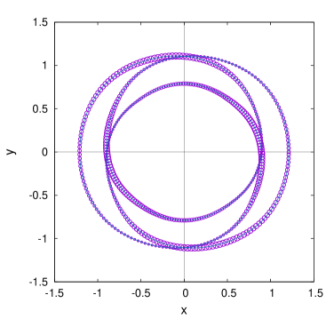
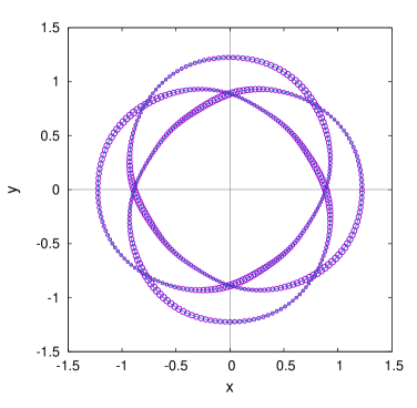
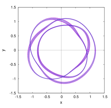
Figure 1: Examples of stable knots at $P=3$, found by simulation of equations (26) with different initial conditions: a) $f(\varphi,0)=0.6[i\cos(2\varphi/3)-0.5\sin(4\varphi/3)]$ — “figure-eight knot”; b) $f(\varphi,0)=0.6[i\cos(4\varphi/3)-0.5\sin(8\varphi/3)]$; c) $f(\varphi,0)=0.6i\{\cos(\varphi/3)+\exp(11i\varphi/3)[1+\cos(2[\varphi-\pi]/3)]^{4}/16\}$ — “granny knot”. In cases a) and b) the parameters $\lambda=4.0$, $\gamma=0$. In case c) $\gamma=1.5$, $\lambda=\gamma^{2}/2+4.5$.

But it would be a mistake to believe that, having taken arbitrary initial data $f_{n}(\varphi,\tau=0)$, we can integrate the gradient equations to very long $\tau$ with conservation of initial topology of the knot, and that in the limit $\tau\to+\infty$ we will inevitably get some smooth functions $f_{n}\to\theta_{n}$. On the contrary, it is quite possible that after a finite “time”, a singularity will develop in system (26), when $\delta(\tau)\equiv\mbox{min}_{\varphi}|f_{j}(\varphi,\tau)-f_{l}(\varphi,\tau)|\to 0$ at $\tau\to\tau_{\rm sing}$. Numerical discretization of the curve will result in a self-intersection, and topology will change at that event. In other words, a dispersive tendency towards smoothing of locally twisted filaments can prevail over their mutual repulsion. Indeed, when a typical scale along $\varphi$ becomes of order $\delta$, then the dispersive term $f_{\varphi\varphi}$ has the same order $1/\delta$ as the nonlinear term. Therefore the question remains open, if a stationary solution always exists at a given knot topology.

But nevertheless, in many cases $\delta(\tau)$ does not go to zero, topology of initial knot is conserved, and smooth solutions are found successfully (sometimes, however, the “relaxation” to a minimum of $\tilde{H}_{0}$ occurs rather slowly).

We also mention a possible case $\alpha<0$, when function $r\rho(z,r)$ has a minimum at point $z=0$, $r=1$ instead of maximum. In that case at $\epsilon\neq 0$ the integrals $N_{\sigma}$ are absent, but the functional $H-\gamma M$ itself is bounded from below. Therefore stable rotating around $z$-axis knots of the form $W_{n}=F_{n}(\varphi-\gamma t)$ exist.

Another noteworthy result is about numerical simulations of equations of motion. It turns out that also conservative system (21) can exhibit a tendency towards a finite-time singularity, not only the gradient system (26). An appropriate example is given in Fig.2. In the framework of the Gross-Pitaevskii equation, such a rapid collision of vortex lines typically results in their re-connection. Of course, our simplified equations loose their literal applicability closely to the singularity, but an initial stage of its formation is described correctly. Clarification of collapse conditions and its relation to vortex knot topology are interesting tasks for future research.

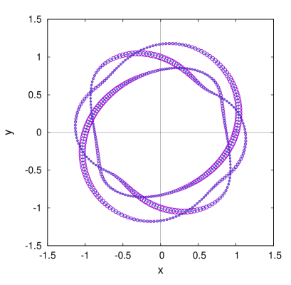
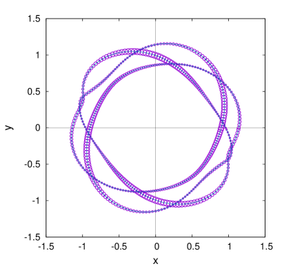
Figure 2: A tendency towards finite-time singularity in Eqs.(21): a) initial knot configuration obtained by simulation of auxiliary system (26) (with parameters $\gamma=0.7$, $\lambda=\gamma^{2}/2+4.0$) to $\tau_{\rm max}=7.0$, with initial conditions $f(\varphi,0)=0.6[\exp(2i\varphi/3)+\exp(4i\varphi/3)+\exp(8i\varphi/3)]$; b) the knot at $t=2.3$ with locally convergent parts of the filament [shown without taking into account the phase factor $\exp(i\alpha t/2)$].

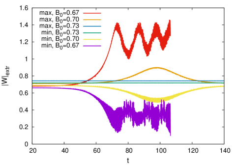
Figure 3: Examples of the dynamics of extreme deviations for stable and unstable solutions (30).

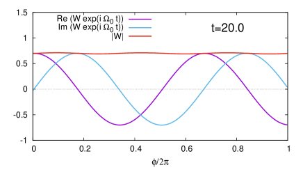
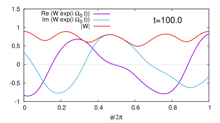
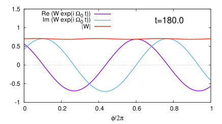
Figure 4: Growth and subsequent decay of unstable mode at $\alpha=2.8$, $\epsilon=0.2$, $B_{0}=0.7$.

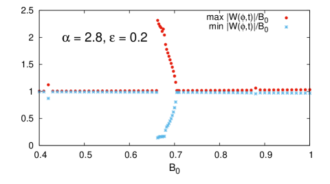
Figure 5: Structure of stable and unstable bands at $\alpha=2.8$, $\epsilon=0.2$. One strongly unstable band is seen near $B_{0}=0.66$, and two weakly unstable bands are near $B_{0}=0.42$ and $B_{0}=0.88$.

IV Case $P=2$

Let us now consider in more detail the simplest vortex configurations with $P=2$. Introducing the sum $w=W_{0}+W_{1}$ and the difference $W=W_{0}-W_{1}$, we obtain two “un-linked” equations: Eq.(19) and

$$iW_{t}=-\frac{1}{2}(W_{\varphi\varphi}+\alpha W-\epsilon W^{*})-\frac{2}{W^{*}},$$ (27)

the last one with anti-periodic boundary conditions. Let us concentrate our attention on this equation. In the case $\epsilon=0$, exact solutions exist of the form

$$W=B_{0}\exp(ik_{0}\varphi-i\Omega_{0}t+i\zeta_{0}),$$ (28)

depending on a real parameter $B_{0}>0$, where

$$\Omega_{0}=\frac{1}{2}(k_{0}^{2}-\alpha)-\frac{2}{B_{0}^{2}},$$ (29)

and $k_{0}$ should be a half-integer $Q/2$ (at $k_{0}=3/2$ the solution corresponds to “trefoil” ${\cal T}_{2,3}$). It is not difficult to analyze small perturbations and make sure that the given solution is stable at all $B_{0}$ and $\alpha$.

Situation is more complicated when $\epsilon\neq 0$. In that case there are stationary solutions as well. At small $\epsilon$ up to the first-order accuracy we easily obtain

$$W\approx B_{0}\exp(i\zeta)+\epsilon C\exp(-i\zeta)+\epsilon D\exp(3i\zeta),$$ (30)

where $\zeta=k_{0}\varphi-\Omega_{0}t+\zeta_{0}$, and coefficients $C$ and $D$ satisfy a linear system of equations

$$-\Omega_{0}C = \frac{1}{2}(k_{0}^{2}-\alpha)C+\frac{2}{B_{0}^{2}}D+\frac{B_{0}}{2},$$ (31)

$$3\Omega_{0}D = \frac{1}{2}(9k_{0}^{2}-\alpha)D+\frac{2}{B_{0}^{2}}C.$$ (32)

The solution of this system is

$$D=B_{0}/J,\qquad C=-B_{0}^{3}(3k_{0}^{2}+\alpha+6/B_{0}^{2})/(2J),$$ (33)

$$J=-4/B_{0}^{2}+B_{0}^{2}(k_{0}^{2}-\alpha-2/B_{0}^{2})(3k_{0}^{2}+\alpha+6/B_{0}^{2}).$$ (34)

A difference in comparison to the case $\epsilon=0$ is that at some relations between $B_{0}$ and $\alpha$, parametric resonances turn out be possible in the dynamical system under consideration, thus resulting in instabilities. In other words, with small random initial perturbations near the stationary solution, three possible scenarios can develop in subsequent dynamics of the largest and the smallest values of $|W|$. When solution (30) is stable, $|W|_{\rm max,min}$ do not exhibit considerable changes. But if (30) is unstable then deviations of $|W|$ first grow exponentially, and after that either return closely to initial small values or the system passes to a quasi-turbulent regime. For illustration, in Fig.3 examples of numerically found temporal dependencies of extreme quantities $\mbox{max}_{\varphi}|W(\varphi,t)|$ and $\mbox{min}_{\varphi}|W(\varphi,t)|$ are given at $\alpha=2.8$, $\epsilon=0.2$ for several $B_{0}$. Fig.4 shows how the solution looks at recurrent dynamics of unstable mode.

If in each such numerical simulation on a sufficiently long time interval we record globally reached extreme values of quantity $|W|/B_{0}$, and after that we draw their dependencies on $B_{0}$, then a structure of stable and unstable bands at fixed $\alpha$ and $\epsilon$ is obtained. An example is given in Fig.5. It is important that with rather small $\epsilon$, stable bands dominate.

V Conclusions

Thus, in this work for the first time relatively simple and convenient for analytical study and for numerical modeling, Hamiltonian equations have been derived which are able to describe in a definite limit the dynamics of knotted quantum vortex lines in spatially nonuniform axisymmetric Bose-Einstein condensates in the Thomas-Fermi regime at zero temperature. In numerical experiments, in a number of cases, a tendency towards a finite-time singularity was observed for knots with nontrivial topology. In the framework of suggested model, at definite values of parameters, stable stationary solutions with different topology have been found, with no analogs in uniform condensates. It has been revealed that in general case, solutions in the form of torus knots can be parametrically unstable but unstable bands are relatively narrow at small anisotropy of the maximum of function $r\rho(z,r)$, in the vicinity of which all the dynamics occurs.

Our theory is heavily based upon a large parameter $\Lambda$ which however can hardly be very large in reality. Therefore, it seems very desirable to compare in the future the predictions of the present simplified model to results of direct numerical simulation of the Gross-Pitaevskii equation at moderate $\Lambda$.

References

- (1) A. L. Fetter, Rev. Mod. Phys. 81, 647 (2009).
- (2) A. A. Svidzinsky and A. L. Fetter, Phys. Rev. A 62, 063617 (2000).
- (3) A. L. Fetter and A. A. Svidzinsky, J. Phys.: Condens. Matter 13, R135 (2001).
- (4) V. P. Ruban, Phys. Rev. E 64, 036305 (2001).
- (5) A. Aftalion and T. Riviere, Phys. Rev. A 64, 043611 (2001).
- (6) J. Garcia-Ripoll and V. Perez-Garcia, Phys. Rev. A 64, 053611 (2001).
- (7) J. R. Anglin, Phys. Rev. A 65, 063611 (2002).
- (8) A. Aftalion and R. L. Jerrard, Phys. Rev. A 66, 023611 (2002).
- (9) P. Rosenbusch, V. Bretin, and J. Dalibard, Phys. Rev. Lett. 89, 200403 (2002).
- (10) A. Aftalion and I. Danaila, Phys. Rev. A 68, 023603 (2003).
- (11) A. Aftalion and I. Danaila, Phys. Rev. A 69, 033608 (2004).
- (12) D. E. Sheehy and L. Radzihovsky, Phys. Rev. A 70, 063620 (2004).
- (13) I. Danaila, Phys. Rev. A 72, 013605 (2005).
- (14) A. Fetter, Phys. Rev. A 69, 043617 (2004).
- (15) T.-L. Horng, S.-C. Gou, and T.-C. Lin, Phys. Rev. A 74, 041603 (2006).
- (16) S. Serafini, M. Barbiero, M. Debortoli, S. Donadello, F. Larcher, F. Dalfovo, G. Lamporesi, and G. Ferrari, Phys. Rev. Lett. 115, 170402 (2015).
- (17) S. Serafini, L. Galantucci, E. Iseni, T. Bienaime, R. N. Bisset, C. F. Barenghi, F. Dalfovo, G. Lamporesi, and G. Ferrari, Phys. Rev. X 7, 021031 (2017).
- (18) R. N. Bisset, S. Serafini, E. Iseni, M. Barbiero, T. Bienaime, G. Lamporesi, G. Ferrari, and F. Dalfovo, Phys. Rev. A 96, 053605 (2017).
- (19) R. L. Ricca, D. C. Samuels, and C. F. Barenghi, J. Fluid Mech. 391, 29 (1999).
- (20) F. Maggioni, S. Alamri, C. F. Barenghi, and R. L. Ricca, Phys. Rev. E 82, 026309 (2010).
- (21) D. Proment, M. Onorato, and C. F. Barenghi, Phys. Rev. E 85, 036306 (2012).
- (22) D. Kleckner and W. T. M. Irvine, Nature Physics 9, 253 (2013).
- (23) D. Proment, M. Onorato, and C. F. Barenghi, J. Phys.: Conf. Ser. 544, 012022, (2014).
- (24) P. Clark di Leoni, P. D. Mininni, and M. E. Brachet, Phys. Rev. A 94, 043605 (2016).
- (25) D. Kleckner, L. H. Kauffman, and W. T. M. Irvine, Nature Physics 12, 650 (2016).
- (26) M. D. Bustamante and S. Nazarenko, Phys. Rev. E 92, 053019 (2015).
- (27) V. P. Ruban, JETP Letters 105, 458 (2017).
- (28) V. P. Ruban, JETP 124, 932 (2017).
- (29) H. Hasimoto, J. Fluid Mech. 51, 477 (1972).
- (30) V. P. Ruban, JETP Letters 103, 780 (2016).
- (31) V. P. Ruban, JETP Letters 104, 868 (2016).
- (32) V. P. Ruban, JETP Letters 106, 223 (2017).
- (33) V. E. Zakharov, Usp. Fiz. Nauk 155, 529 (1988).
- (34) R. Klein, A. J. Majda, and K. Damodaran, J. Fluid Mech. 288, 201 (1995).
- (35) C. E. Kenig, G. Ponce, and L. Vega, Commun. Math. Phys. 243, 471 (2003).
- (36) N. Hietala, R. Hanninen, H. Salman, and C. F. Barenghi, Phys. Rev. Fluids 1, 084501 (2016).