Inferences on the Higgs Boson and Axion Masses
through a Maximum Entropy Principle

Abstract

The Maximum Entropy Principle (MEP) is a method that can be used to infer the value of an unknown quantity in a set of probability functions. In this work we review two applications of MEP: one giving a precise inference of the Higgs boson mass value; and the other one allowing to infer the mass of the axion. In particular, for the axion we assume that it has a decay channel into pairs of neutrinos, in addition to the decay into two photons. The Shannon entropy associated to an initial ensemble of axions decaying into photons and neutrinos is then built for maximization.

The Method of Maximum Entropy Principle

Among the biggest challenges of physics is to find an explanation for the values of the masses of the elementary particles. With the discovery of the Higgs boson at the LHC, and the measurements of its properties, we have now the experimental evidence that the mechanism of spontaneous symmetry breaking is effectively behind the mass generation for the elementary particles, as implemented in the Standard Model (SM). Although this represented an invaluable advance for understanding of subatomic physics, the spontaneous symmetry breaking mechanism in the SM does not determine the value of the masses of the elementary particles, except for the photon which is correctly left massless and all the neutrinos which are incorrectly left massless. It means that some still missing mechanism must supplement, or totally replace, the spontaneous symmetry breaking in order to allow a full determination of the masses of the elementary particles.

In particular, for the Higgs boson some ideas have arised relating its mass to the maximum of a probability distribution built from the branching ratios [1], [2]. As observed in Ref. [1] a probability distribution function constructed multiplying the main branching ratios for the SM Higgs boson decay has a peak near to the measured value $M_{H}\approx 125$ GeV. This could be connected to some sort of entropy so that such a mass value maximizes, simultaneously, the decay probabilities into all SM particles. In the work of Ref. [2] we presented a development based on the Shannon entropy built with the Higgs boson branching ratios, showing that the value of the Higgs boson mass follows from a Maximum Entropy Principle (MEP).

In the following we present a short review of our MEP method to infer the mass of the SM Higgs boson. After that we also review an application of MEP for inferring the mass of the axion assuming a specific low energy effective Lagrangian [3].

Inferring the Higgs boson mass

Consider an initial state of $N$ Higgs bosons that evolves, through decay, to a final state composed by many different particles as represented in Fig. 1. After a time $\tau\gg 1/\Gamma_{total}$ the system transforms into a thermal bath of particles from the Higgs boson decays, according to its branching ratios $BR_{k}(M_{H}|\boldsymbol{\theta})={\Gamma_{k}(M_{H}|\boldsymbol{\theta})}/{\Gamma_{total}(M_{H}|\boldsymbol{\theta})}$, where $k=\gamma\gamma,\;gg,\;Z\gamma,\;q\bar{q},\;\ell^{+}\ell^{-}$, $WW^{*},\;ZZ^{*}$, are the 14 main SM decay modes; and $\boldsymbol{\theta}$ represents all the other predetermined parameters entering into the formula; $\Gamma_{k}(M_{H}|\boldsymbol{\theta})$ and $\Gamma_{total}(M_{H}|\boldsymbol{\theta})$ are the partial and the total Higgs boson widths, respectively. The probability that the $N$ Higgs bosons system evolve to a given final state of a bath of Standard Model particles, defined by a partition of $n_{1}$ particles decaying into the mode $1$, $n_{2}$ particles decaying into the mode $2$, and so on until $n_{m}$ particles decaying into the mode $m$, is given by

$$\hskip 8.5359ptP(\{n_{k}\}_{k=1}^{m})\equiv\frac{N!}{n_{1}!\cdots n_{m}!}\prod_{k=1}^{m}\left[BR_{k}(M_{H}|\boldsymbol{\theta})\right]^{n_{k}},$$ (1)

in which $\sum_{i}n_{i}=N$.

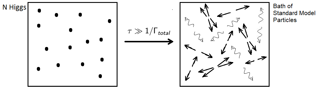
Figure 1: System of $N$ Higgs boson decaying into a bath of Standard Model particles.

We define the Shannon entropy [4] associated to the decay of the system of $N$ Higgs bosons summing over each possible partition as

$$S_{N}=-\sum_{\{n\}}^{N}P(\{n_{k}\}_{k=1}^{m})\;\ln\left[P(\{n_{k}\}_{k=1}^{m})\right]=-\langle\ln(P)\rangle.$$ (2)

It can be shown, taking the asymptotic limit $N\rightarrow\infty$ formula for $S_{N}$ [5], that maximization of $S_{N}$ is equivalent to the maximization of

$$S_{\infty}(M_{H}|\boldsymbol{\theta})=\ln\left(\prod_{k=1}^{m}BR_{k}(M_{H}|\boldsymbol{\theta})\right)$$ (3)

The expression in Eq. (3) is in fact the log-likelihood from the product of the branching ratios. Thus, we see as an outcome of MEP that the simultaneous maximization of the Higgs boson decays into Standard Model particles is equivalent to the maximization of the log-likelihood.

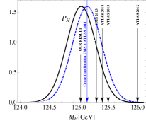
Figure 2: Probability distribution function $P(M_{H})$ obtained in [2] from the maximum solution of $S_{\infty}$ is shown in the black curve.

Taking into account several sets of values within the experimental errors in the Standard Model electroweak parameters $\boldsymbol{\theta}$ [6], a gaussian probability distribution function, $P_{H}(\hat{M}_{H})$, is then fitted with the maximum solutions, $\hat{M}_{H}$, of $S_{\infty}(M_{H}|\boldsymbol{\theta})$. The result is shown in Fig. 2. The peak of $P_{H}(\hat{M}_{H})$ is interpreted as the most probable value for the mass of the SM Higgs boson derived from MEP. Such a peak occurs for $M_{H}^{th}=125.04\pm 0.25\;\hbox{GeV}$, and reflects the combined uncertainties over the SM parameters. It must be pointed out that this mass value determined from MEP is almost identical to the latest experimental value $M_{H}^{exp}=125.09\pm 0.21\,(stat.)\,\pm 0.11\,(syst.)\,{\rm GeV}$  [7].

Inferring the axion mass

We now review an application of MEP for inferring the mass of the hypothetical axion under two general assumptions. First, the axion can decay into pairs of neutrinos, in addition to the typical two photons decay channel. Second, the effective Lagrangian describing the axion field, $A(x)$, interactions with the electromagnetic strength tensor, $F^{\mu\nu}$, and neutrinos fields, $\nu_{i}$, is

$$\mathscr{L}_{eff}=\frac{1}{2}\partial_{\mu}A\,\partial^{\mu}A-\frac{1}{2}m_{A}^{2}\,A^{2}-\frac{g_{A\gamma}}{4}\,A\,F^{\mu\nu}{\widetilde{F}}_{\mu\nu}-\frac{g_{A\nu}}{2}\,\overline{\nu}_{i}\gamma^{\mu}\gamma_{5}\nu_{i}\,\partial_{\mu}A\,,$$ (4)

where $i=1,\,2,\,3$, and ${\widetilde{F}}_{\mu\nu}=\frac{1}{2}\epsilon_{\mu\nu\sigma\rho}F^{\sigma\rho}$. The axion-photon and the axion-neutrinos couplings are defined in terms of the axion decay constant, $f_{A}$, the fine structure constant, $\alpha$, and the order 1 model dependent anomaly coefficients, $C_{A\nu}$, ${\widetilde{C}}_{A\gamma}$, as $g_{A\gamma}={\alpha{\widetilde{C}}_{A\gamma}}/{2\pi f_{A}}$ and $g_{A\nu}={C_{A\nu}}/{f_{A}}$. The effective Lagrangian in Eq. (4) can be derived from a kind of DFSZ axion model with the addition of right-handed neutrinos [3]. It can be seen that the axion branching ratios $BR_{A\rightarrow\gamma\gamma}$ and $BR_{A\rightarrow\nu_{i}\nu_{i}}$ computed with Eq. (4) depend only on the ratio $C_{A\nu}/{\widetilde{C}}_{A\gamma}$, the mass of the axion, $m_{A}$, and the lightest neutrino mass, $m_{1}$.

The neutrinos squared mass differences, $\Delta m_{12}^{2}=m_{2}^{2}-m_{1}^{2}=(7.45\pm 0.25)\times 10^{-5}\,\mathrm{eV}^{2}$ and $\Delta m_{31}^{2}=m_{3}^{2}-m_{1}^{2}=(2.55\pm 0.05)\times 10^{-3}\,\mathrm{eV}^{2}$  [8], assuming the normal hierarchy, enter as a prior information for the maximization of $S(m_{A}|m_{1},r_{\nu})=\ln\left(BR_{0}BR_{1}BR_{2}BR_{3}\right)$. Still, there is the bound on the sum of neutrinos masses $0.059\text{ eV}<\sum_{i}m_{i}<0.23\;\text{eV}$, from the measurements of cosmic microwave background anisotropies [9], implying that $0\leq m_{1}<0.0712\;\text{eV}$.

It is shown in green on Fig. 3 the maximum points of the entropy $S(m_{A}|m_{1},r_{\nu})$. The boundaries given by the gray curves are defined by the largest (upper) and lowest (lower) allowed value of $m_{1}$. For the DFSZ model with right-handed neutrinos the anomaly coefficients are such that $r_{\nu}<0.46$ and the region beyond the red dashed line in Fig. 3 is excluded. Taking into account the astrophysical bounds from red giants [10] we obtain $r_{\nu}<0.034$, excluding the region beyond the green dashed line in Fig. 3, and this implies that $0.1$ eV $<m_{A}<6.3$ eV.

A more strong inference can be made maximizing the entropy as being a function of three unknowns, i. e., $S\equiv S(m_{A},m_{1},r_{\nu})$. In this case we have a more sharp prediction of $0.1$ eV $<m_{A}<0.2$ eV, which is represented with the blue line in Fig. 3.

Finally, supposing that the axion can decay only into a pair of the lightest neutrino the inference made with MEP is a linear relation between $m_{A}$ and $m_{1}$, with the proportionality coefficient depending on $r_{\nu}$.

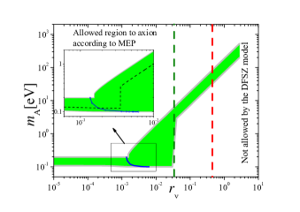
Figure 3: Green region represents the maximum points of $S(m_{A}|m_{1},r_{\nu})$ as obtained in Ref. [3].

Acknowledgments: The authors thank CNPq and Fapesp. A. G. D. also thanks the organizers of Patras 2017 workshop, in special Hero and Konstantin Zioutas for their hospitality.

References

- [1] D. d’Enterria, “On the Gaussian peak of the product of decay probabilities of the standard model Higgs boson at a mass 125 GeV,” arXiv:1208.1993 [hep-ph].
- [2] A. Alves, A. G. Dias and R. da Silva, “Maximum Entropy Principle and the Higgs Boson Mass,” Physica A 420, 1 (2015) [arXiv:1408.0827 [hep-ph]].
- [3] A. Alves, A. G. Dias and R. Silva, “Maximum Entropy Inferences on the Axion Mass in Models with Axion-Neutrino Interaction,” Braz. J. Phys. 47, no. 4, 426 (2017) [arXiv:1703.02061 [hep-ph]].
- [4] C. E. Shannon, “A mathematical theory of communication,” Bell Syst. Tech. J. 27, 379 (1948) [Bell Syst. Tech. J. 27, 623 (1948)].
- [5] J. Cichon and Z. Golebiewski, 23rd International Meeting on Probabilistic, Combinatorial and Asymptotic Methods for the Analysis of Algorithms, http://luc.devroye.org/AofA2012-CfP.html.
- [6] S. Dawson et al., “Working Group Report: Higgs Boson,” arXiv:1310.8361 [hep-ex].
- [7] G. Aad et al. [ATLAS and CMS Collaborations], “Combined Measurement of the Higgs Boson Mass in Collisions at and 8 TeV with the ATLAS and CMS Experiments,” Phys. Rev. Lett. 114, 191803 (2015) [arXiv:1503.07589 [hep-ex]].
- [8] S. F. King, “Unified Models of Neutrinos, Flavour and CP Violation,” Prog. Part. Nucl. Phys. 94, 217 (2017) [arXiv:1701.04413 [hep-ph]].
- [9] P. A. R. Ade et al. [Planck Collaboration], “Planck 2015 results. XIII. Cosmological parameters,” Astron. Astrophys. 594, A13 (2016) [arXiv:1502.01589 [astro-ph.CO]].
- [10] N. Viaux, M. Catelan, P. B. Stetson, G. Raffelt, J. Redondo, A. A. R. Valcarce and A. Weiss, “Neutrino and axion bounds from the globular cluster M5 (NGC 5904),” Phys. Rev. Lett. 111, 231301 (2013) [arXiv:1311.1669 [astro-ph.SR]].