Partial Homology Relations - Satisfiability in terms of Di-Cographs

Abstract

Directed cographs (di-cographs) play a crucial role in the reconstruction of evolutionary histories of genes based on homology relations which are binary relations between genes. A variety of methods based on pairwise sequence comparisons can be used to infer such homology relations (e.g. orthology, paralogy, xenology). They are satisfiable if the relations can be explained by an event-labeled gene tree, i.e., they can simultaneously co-exist in an evolutionary history of the underlying genes. Every gene tree is equivalently interpreted as a so-called cotree that entirely encodes the structure of a di-cograph. Thus, satisfiable homology relations must necessarily form a di-cograph. The inferred homology relations might not cover each pair of genes and thus, provide only partial knowledge on the full set of homology relations. Moreover, for particular pairs of genes, it might be known with a high degree of certainty that they are not orthologs (resp. paralogs, xenologs) which yields forbidden pairs of genes. Motivated by this observation, we characterize (partial) satisfiable homology relations with or without forbidden gene pairs, provide a quadratic-time algorithm for their recognition and for the computation of a cotree that explains the given relations.

1 Introduction

Directed cographs (di-cographs) are a well-studied class of graphs that can uniquely be represented by an ordered rooted tree $(T,t)$, called cotree, where each inner vertex gets a unique label “$1$”, “$\overrightarrow{1}$” or “$0$” [5, 7, 9, 12]. In particular, di-cographs have been shown to play an important role for the reconstruction of the evolutionary history of genes or species based on genomic sequence data [18, 17, 20, 23, 11, 21]. Genes are the molecular units of heredity holding the information to build and maintain cells. During evolution, they are mutated, duplicated, lost and passed to organisms through speciation or horizontal gene transfer (HGT), which is the exchange of genetic material among co-existing species. A gene family comprises genes sharing a common origin. Genes within a gene family are called homologs.

The history of a gene family is equivalent to an event-labeled gene tree, the leaves correspond to extant genes, internal vertices to ancestral genes and the label of an internal vertex highlighting the event at the origin of the divergence leading to the offspring, namely speciation-, duplication- or HGT-events [13]. Equivalently, the history of genes is described by an event-labeled rooted tree for which each inner vertex gets a unique label “$1$” (for speciation) , “$0$” (for duplication) or “$\overrightarrow{1}$” (for HGT). In other words, any gene tree is also a cotree. The type of event “$1$”, “$0$” and “$\overrightarrow{1}$” of the lowest common ancestor of two genes gives rise to one of three distinct homology relations respectively, the orthology-relation $R_{1}$, the paralogy-relation $R_{0}$ and the xenology-relation $R_{\overrightarrow{1}}$. The orthology-relation $R_{1}$ on a set of genes forms an undirected cograph [17]. In [18] it has been shown that the graph $G$ with arc set $E(G)=R_{1}\cup R_{\overrightarrow{1}}$ must be a di-cograph (see [19] for a detailed discussion).

In practice, these homology relations are often estimated from sequence similarities and synteny information, without requiring any a priori knowledge on the topology of either the gene tree or the species tree (see e.g. [1, 2, 3, 6, 25, 26, 29, 33, 34, 10, 24, 30]). The starting point of this contribution is a set of estimated relations $R_{1}$, $R_{\overrightarrow{1}}$ and $R_{0}$. In particular, we consider so-called partial and forbidden relations: In fact, similarity-based homology inference methods often depend on particular threshold parameters to determine whether a given pair of genes is in one of $R_{0},R_{1}$ or $R_{\overrightarrow{1}}$. Gene pairs whose sequence similarity falls below (or above) a certain threshold cannot be unambiguously identified as belonging to one of the considered homology relations. Hence, in practice one usually obtains partial relations only, as only subsets of these relations may be known. Moreover, different homology inference methods may lead to different predictions. Thus, instead of a yes or no orthology, paralogy or xenology assignment, a confidence score can rather be assigned to each relation [11]. A simple way of handling such weighted gene pairs is to set an upper threshold above which a relation is predicted, and a lower threshold under which a relation is rejected, leading to partial relations with forbidden gene pairs, i.e., gene pairs that are not included in any of the three relations but for which it is additionally known to which relations they definitely not belong to.

In this contribution, we generalize results established by Lafond and El-Mabrouk [22] and characterize satisfiable partial relations with and without forbidden relations. We provide a recursive quadratic-time algorithm testing whether the considered relations are satisfiable, and if so reconstructing a corresponding cotree. This, in turn, allows us to extend satisfiable partial relations to full relations. Finally, we evaluate the accuracy of the designed algorithm on large-scaled simulated data sets. As it turns out, it suffices to have only a very few but correct pairs of relations to recover most of them.

Note, the results established here may also be of interest for a broader scientific community. Di-cographs play an important role in computer science because many combinatorial optimization problems that are NP-complete for arbitrary graphs become polynomial-time solvable on di-cographs [8, 5, 14]. However, the cograph-editing problem is NP-hard [27]. Thus, an attractive starting point for heuristics that edit a given graph to a cograph may be the knowledge of satisfiable parts that eventually lead to partial information of the underlying di-cograph structure of the graph of interest.

2 Preliminaries

Basics.

In what follows, we always consider binary and irreflexive relations $R\subseteq V^{\times}_{\mathrm{irr}}\coloneqq V\times V\setminus\{(v,v)\mid v\in V\}$ and we omit to mention it each time. If we have a non-symmetric relation $R$, then we denote $R^{\mathrm{sym}}=R\cup\{(x,y)\mid(y,x)\in R\}$ the symmetric extension of $R$ and by $\overleftarrow{R}$ the set $\{(x,y)\mid(y,x)\in R\}$. For a subset $W\subseteq V$ and a relation $R$, we define $R[W]=\{(x,y)\in R\mid x,y\in W\}$ as the sub-relation of $R$ that is induced by $W$. Moreover, for a set of relations $\mathcal{R}=\{R_{1},\dots,R_{n}\}$ we set $\mathcal{R}[W]=\{R_{1}[W],\dots,R_{n}[W]\}$.

A directed graph (digraph) $G=(V,E)$ has vertex set $V(G)=V$ and arc set $E(G)=E\subseteq V^{\times}_{\mathrm{irr}}$. Given two disjoint digraphs $G=(V,E)$ and $H=(W,F)$, the digraph $G\cup H=(V\cup W,E\cup F)$, $G\oplus H=(V\cup W,E\cup F\cup\{(x,y),(y,x)\mid x\in V,y\in W\})$ and $G\oslash H=(V\cup W,E\cup F\cup\{(x,y)\mid x\in V,y\in W\})$ denote the union, join and directed join of $G$ and $H$, respectively. For a given subset $W\subseteq V$, the induced subgraph $G[W]=(W,F)$ of $G=(V,E)$ is the subgraph for which $x,y\in W$ and $(x,y)\in E$ implies that $(x,y)\in F$. We call $W\subseteq V$ a (strongly) connected component of $G=(V,E)$ if $G[W]$ is a maximal (strongly) connected subgraph of $G$.

Given a digraph $G=(V,E)$ and a partition $\{V_{1},V_{2},\dots,V_{k}\}$ of its vertex set $V$, the quotient digraph $G/\{V_{1},V_{2},\dots,V_{k}\}$ has as vertex set $\{V_{1},V_{2},\dots,V_{k}\}$ and two distinct vertices $V_{i},V_{j}$ form an arc $(V_{i},V_{j})$ in $G/\{V_{1},\dots,V_{k}\}$ if there are vertices $x\in V_{i}$ and $y\in V_{j}$ with $(x,y)\in E$.

An acyclic digraph is called DAG. It is well-known that the vertices of a DAG can be topologically ordered, i.e., there is an ordering of the vertices as $v_{1},\dots,v_{n}$ such that $(v_{i},v_{j})\in E$ implies that $i<j$. To check whether a digraph $G$ contains no cycles one can equivalently check whether there is a topological order, which can be done via a depth-first search in $O(|V(G)|+|E(G)|)$ time.

Furthermore, we consider a rooted tree $T=(W,E)$ (on $V$) with root $\rho_{T}\in V$ and leaf set $V\subseteq W$ such that the root has degree $\geq 2$ and each vertex $v\in W\setminus V$ with $v\neq\rho_{T}$ has degree $\geq 3$. We write $x\succeq_{T}y$, if $x$ lies on the path from $\rho_{T}$ to $y$. The children of a vertex $x$ are all adjacent vertices $y$ for which $x\succeq_{T}y$. Given two leaves $x,y\in V$, their lowest common ancestor $\operatorname{lca}(x,y)$ is the first vertex that lies on both paths from $x$ to the root and $y$ to the root. We say that rooted trees $T_{1},\dots,T_{k}$, $k\geq 2$ are joined under a new root in the tree $T$ if $T$ is obtained by the following procedure: add a new root $\rho_{T}$ and all trees $T_{1},\dots,T_{k}$ to $T$ and connect the root $\rho_{T_{i}}$ of each tree $T_{i}$ to $\rho_{T}$ with an edge $(\rho_{T},\rho_{T_{i}})$.

Di-cographs.

Di-cographs generalize the notion of undirected cographs [12, 9, 7, 5] and are defined recursively as follows: The single vertex graph $K_{1}$ is a di-cograph, and if $G$ and $H$ are di-cographs, then $G\cup H$, $G\oplus H$, and $G\oslash H$ are di-cographs [15, 7]. Each Di-cograph $G=(V,E)$ is associated with a unique ordered least-resolved tree $T=(W,F)$ (called cotree) with leaf set $L=V$ and a labeling function $t:W\setminus L\to\{0,1,\overrightarrow{1}\}$ defined by

$$t(\operatorname{lca}(x,y))=\begin{cases}0,&\text{ if }(x,y),(y,x)\notin E\\ 1,&\text{ if }(x,y),(y,x)\in E\\ \overrightarrow{1},&\text{ otherwise.}\end{cases}$$

Since the vertices in the cotree $T$ are ordered, the label $\overrightarrow{1}$ on some $\operatorname{lca}(x,y)$ of two distinct leaves $x,y\in L$ means that there is an arc $(x,y)\in E$, while $(y,x)\notin E$, whenever $x$ is placed to the left of $y$ in $T$.

Some important properties of di-cographs that we need for later reference are given now.

Lemma 1 ([7, 15, 28])

A digraph $G=(V,E)$ is a di-cograph if and only if each induced subgraph of $G$ is a di-cograph.

Determining whether a digraph is a di-cograph, and if so, computing the corresponding cotree can be done in $O(|V|+|E|)$ time.

3 Problem Statement

As argued in the introduction and explained in more detail in [18], the evolutionary history of genes is equivalently described by an ordered rooted tree $\mathcal{T}=({T},{t})$ where the leaf set of ${T}$ are genes and $t$ is a map that assigns to each non-leaf vertex a unique label $0,1$ or $\overrightarrow{1}$. The labels correspond to the classical evolutionary events that act on the genes through evolution, namely speciation ($1$), duplication ($0$) and horizontal gene transfer (HGT) ($\overrightarrow{1}$). The tree $T$ is ordered to represent the inherently asymmetric nature of HGT events with their unambiguous distinction between the vertically transmitted “original” gene and the horizontally transmitted “copy”.

Therefore, a given gene tree $\mathcal{T}=({T},{t})$ is a cotree of some di-cograph $G(\mathcal{T})=(V,E)$. In particular, $\mathcal{T}$ gives rise to the following three well-known homology relations between genes:

the orthology-relation: $$R_{1}({\mathcal{T}})=\{(x,y)\mid t(\operatorname{lca}(x,y))=1\},$$

the paralogy-relation: $$R_{0}({\mathcal{T}})=\{(x,y)\mid t(\operatorname{lca}(x,y))=0\},\text{ and}$$

the xenology-relation: $$R_{\overrightarrow{1}}({\mathcal{T}})=\{(x,y)\mid t(\operatorname{lca}(x,y))=\overrightarrow{1}\text{ and }x\text{ is left of }y\text{ in }T\}.$$

Equivalently, $R_{1}({\mathcal{T}})=\{(x,y)\mid(x,y),(y,x)\in E\}$, $R_{0}({\mathcal{T}})=\{(x,y)\mid(x,y),(y,x)\notin E\}$, $R_{\overrightarrow{1}}({\mathcal{T}})=\{(x,y)\mid(x,y)\in E,(y,x)\notin E\}$. By construction, $R_{1}({\mathcal{T}})$ and $R_{0}({\mathcal{T}})$ are symmetric relations, while $R_{\overrightarrow{1}}({\mathcal{T}})$ is an anti-symmetric relation.

In practice, however, one often has only empirical estimates $R_{0},R_{1}$ and $R_{\overrightarrow{1}}$ of some “true” relations $R_{0}({\mathcal{T}}),R_{1}({\mathcal{T}})$ and $R_{\overrightarrow{1}}({\mathcal{T}})$, respectively. Moreover, it is often the case that for two distinct leaves $x,y$ none of the pairs $(x,y)$ and $(y,x)$ is contained in the estimates $R_{0},R_{1}$ and $R_{\overrightarrow{1}}$.

In what follows we always assume that $R_{0},R_{1}$ and $R_{\overrightarrow{1}}$ are subsets of $V^{\times}_{\mathrm{irr}}$ and pairwisely disjoint. Furthermore $R_{0}$ and $R_{1}$ are always symmetric relations while $R_{\overrightarrow{1}}$ is always an anti-symmetric relation.

Definition 1 (Full and Partial Relations)

A set $\mathcal{H}=\{R_{0},R_{1},R_{\overrightarrow{1}}\}$ of relations is full if $R_{0}\cup R_{1}\cup R_{\overrightarrow{1}}^{\mathrm{sym}}=V^{\times}_{\mathrm{irr}}$ and partial if $R_{0}\cup R_{1}\cup R_{\overrightarrow{1}}^{\mathrm{sym}}\subseteq V^{\times}_{\mathrm{irr}}$.

The definition allows considering full relations as partial. In other words, all results that will be obtained for partial relations will also be valid for full relations.

The question arises under which conditions the given partial relations $R_{0},R_{1}$ and $R_{\overrightarrow{1}}$ are satisfiable, i.e., there is a cotree $\mathcal{T}=(T,t)$ such that $R_{1}\subseteq R_{1}({\mathcal{T}})$, $R_{0}\subseteq R_{0}({\mathcal{T}})$ and $R_{\overrightarrow{1}}\subseteq R_{\overrightarrow{1}}({\mathcal{T}})$, or equivalently, there is a di-cograph $G^{\star}=(V,E^{\star})$ such that $(R_{1}\cup R_{\overrightarrow{1}})\subseteq E^{\star}$ and $R_{0}\cap E^{\star}=\overleftarrow{R_{\overrightarrow{1}}}\cap E^{\star}=\emptyset$.

Definition 2 (Satisfiable Relations)

A full set $\mathcal{H}=\{R_{0},R_{1},R_{\overrightarrow{1}}\}$ is satisfiable, if there is a cotree $\mathcal{T}=({T},{t})$ such that $R_{1}=R_{1}({\mathcal{T}})$, $R_{0}=R_{0}({\mathcal{T}})$ and $R_{\overrightarrow{1}}=R_{\overrightarrow{1}}({\mathcal{T}})$.

A partial set $\mathcal{H}=\{R_{0},R_{1},R_{\overrightarrow{1}}\}$ is satisfiable, if there is a full set $\mathcal{H}^{\star}=\{R^{\star}_{0},R^{\star}_{1},R^{\star}_{\overrightarrow{1}}\}$ that is satisfiable such that $R_{0}\subseteq R^{\star}_{0}$, $R_{1}\subseteq R^{\star}_{1}$, and $R_{\overrightarrow{1}}\subseteq R^{\star}_{\overrightarrow{1}}$.

In this case, we say that $\mathcal{H}$ can be extended to a satisfiable full set $\mathcal{H}^{\star}$ and that $\mathcal{T}$ explains $\mathcal{H}$ and $\mathcal{H}^{\star}$.

It is easy to see that a full set $\mathcal{H}$ is satisfiable if and only if the graph $G(R_{1},R_{\overrightarrow{1}})=(V,R_{1}\cup R_{\overrightarrow{1}})$ is a di-cograph. The latter result has already been observed in [18] and is summarized bellow.

Theorem 3.1 ([18])

The full set $\mathcal{H}=\{R_{0},R_{1},R_{\overrightarrow{1}}\}$ is satisfiable if and only if $G(R_{1},R_{\overrightarrow{1}})=(V,R_{1}\cup R_{\overrightarrow{1}})$ is a di-cograph.

Due to errors and noise in the data, the graph $G(R_{1},R_{\overrightarrow{1}})$ is often not a di-cograph. However, in case that $\mathcal{H}$ is partial, it might be possible to extend $G(R_{1},R_{\overrightarrow{1}})$ to a di-cograph. Moreover, in practice, one often has additional knowledge about the unknown parts of the relations, that is, one may know that a pair $(x,y)$ is not in relation $R_{i}$ for some $i\in\{0,1,\overrightarrow{1}\}$. To be able to model such forbidden pairs, we introduce the concept of satisfiability in terms of forbidden relations.

Definition 3 (Satisfiable Relations w.r.t. Forbidden Relations)

Let $\mathcal{F}=\{F_{0},F_{1},F_{\overrightarrow{1}}\}$ be a partial set of relations. We say that a full set $\mathcal{H}=\{R_{0},R_{1},R_{\overrightarrow{1}}\}$ is satisfiable w.r.t. $\mathcal{F}$ if $\mathcal{H}$ is satisfiable and

$$R_{0}\cap F_{0}=R_{1}\cap F_{1}=R_{\overrightarrow{1}}\cap F_{\overrightarrow{1}}=\emptyset.$$

On the other hand, a partial set $\mathcal{H}=\{R_{0},R_{1},R_{\overrightarrow{1}}\}$ is satisfiable w.r.t. $\mathcal{F}$ if $\mathcal{H}$ can be extended to a full set $\mathcal{H}^{\star}$ that is satisfiable w.r.t. $\mathcal{F}$.

Equivalently, a partial set $\mathcal{H}=\{R_{0},R_{1},R_{\overrightarrow{1}}\}$ is satisfiable w.r.t. $\mathcal{F}$, if there is a cotree $\mathcal{T}=({T},{t})$ such that $R_{0}\subseteq R_{0}(\mathcal{T})$, $R_{1}\subseteq R_{1}(\mathcal{T})$, $R_{\overrightarrow{1}}\subseteq R_{\overrightarrow{1}}(\mathcal{T})$ and $R_{0}(\mathcal{T})\cap F_{0}=R_{1}(\mathcal{T})\cap F_{1}=R(\mathcal{T})_{\overrightarrow{1}}\cap F_{\overrightarrow{1}}=\emptyset$.

4 Satisfiable Relations

In what follows, we consider the problem of deciding whether a partial set $\mathcal{H}$ of relations is satisfiable, and if so, finding an extended full set $\mathcal{H}^{\star}$ of $\mathcal{H}$ and the respective cotree that explains $\mathcal{H}$. Due to space limitation, all proofs are omitted and can be found in the appendix.

Based on results provided by Böcker and Dress [4], the following result has been established for the HGT-free case.

Theorem 4.1 ([22, 17])

Let $R_{\overrightarrow{1}}=\emptyset$ , $F_{0}=F_{1}=\emptyset$ and $F_{\overrightarrow{1}}=V^{\times}_{\mathrm{irr}}$. A full set $\mathcal{H}=\{R_{0},R_{1},R_{\overrightarrow{1}}\}$ is satisfiable w.r.t. $\mathcal{F}=\{F_{0},F_{1},F_{\overrightarrow{1}}\}$ if and only if the graph $G=(V,R_{1})$ is an undirected cograph.

A partial set $\mathcal{H}=\{R_{0},R_{1},\emptyset\}$ is satisfiable w.r.t. $\mathcal{F}$ if and only if at least one of the following statements is satisfied:

1. $G=(V,R_{1})$ is disconnected and each of its connected components is satisfiable.

2. $G=(V,R_{0})$ is disconnected and each of its connected components is satisfiable.

To generalize the latter result for non-empty relations $R_{\overrightarrow{1}},F_{0}$ and $F_{1}$ and to allow pairs to be added to $R_{\overrightarrow{1}}$, i.e., $F_{\overrightarrow{1}}\neq V^{\times}_{\mathrm{irr}}$, we need the following result.

Lemma 2

A partial set $\mathcal{H}=\{R_{0},R_{1},R_{\overrightarrow{1}}\}$ is satisfiable w.r.t. the set of forbidden relations $\mathcal{F}=\{F_{1},F_{0},F_{\overrightarrow{1}}\}$ if and only if for any partition $\{C_{1},\dots,C_{k}\}$ of $V$ the set $\mathcal{H}[C_{i}]$ is satisfiable w.r.t. $\mathcal{F}[C_{i}]$, $1\leq i\leq k$.

Lemma 2 characterizes satisfiable partial sets $\mathcal{H}=\{R_{0},R_{1},R_{\overrightarrow{1}}\}$ in terms of a partition $\{C_{1},\dots,C_{k}\}$ of $V$ and the induced sub-relations in $\mathcal{H}[C_{i}]$. In what follows, we say that a component $C$ of a graph is satisfiable if the set $\mathcal{H}[C]$ is satisfiable w.r.t. $\mathcal{F}[C]$.

We are now able to state the main result.

Theorem 4.2

Let $\mathcal{H}=\{R_{0},R_{1},R_{\overrightarrow{1}}\}$ be a partial set. Then, $\mathcal{H}$ is satisfiable w.r.t.  the set of forbidden relations $\mathcal{F}=\{F_{0},F_{1},F_{\overrightarrow{1}}\}$ if and only if $R_{0}\cap F_{0}=R_{1}\cap F_{1}=R_{\overrightarrow{1}}\cap F_{\overrightarrow{1}}=\emptyset$ and at least one of the following statements hold:

Rule (0):  $|V|=1$.

Rule (1):  (a) $G_{0}\coloneqq(V,R_{1}\cup R_{\overrightarrow{1}}\cup F_{0})$ is disconnected and (b) each connected component of $G_{0}$ is satisfiable.

Rule (2):  (a) $G_{1}\coloneqq(V,R_{0}\cup R_{\overrightarrow{1}}\cup F_{1})$ is disconnected and (b) each connected component of $G_{1}$ is satisfiable.

Rule (3):  (a) $G_{\overrightarrow{1}}\coloneqq(V,R_{0}\cup R_{1}\cup R_{\overrightarrow{1}}\cup\overleftarrow{F_{\overrightarrow{1}}})$ contains more than one strongly connected component, and (b) each strongly connected component of $G_{\overrightarrow{1}}$ is satisfiable.

Note, the notation $G_{0}$, $G_{1}$ and $G_{\overrightarrow{1}}$ in Thm. 4.2 is chosen because if $G_{0}$ (resp. $G_{1}$ and $G_{\overrightarrow{1}}$) satisfies Rule (1) (resp. (2) and (3)), then the root of the cotree that explains $\mathcal{H}$ is labeled “$0$” (resp. “$1$” and “$\overrightarrow{1}$”).

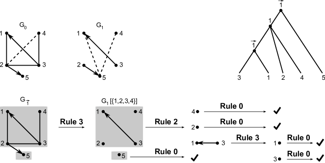
Figure 1: Consider the partial relations $R_{0}=\emptyset$, $R_{1}=\{[1,2],[2,3],[3,4]\}$, and $R_{\overrightarrow{1}}=\{(3,1),(2,5)\}$, and the forbidden relations $F_{0}=\{[2,4]\}$, $F_{1}=\{[1,5],[4,5]\}$ and $F_{\overrightarrow{1}}=\emptyset$. Here $[x,y]\in R$ means that both $(x,y)$ and $(y,x)$ are contained in $R$. Left, the three graphs $G_{0},G_{1}$ and $G_{\overrightarrow{1}}$ as defined in Thm. 4.2 are shown (arrows are omitted for symmetric arcs and dashed arcs correspond to forbidden pairs). Both $G_{0}$ and $G_{1}$ are connected. However, $G_{\overrightarrow{1}}$ contains the two strongly connected components $C_{1}=\{1,2,3,4\}$ and $C_{2}=\{5\}$ (highlighted with gray rectangles). Thus, Rule (3) can be applied. The graphs $G_{0}[C_{1}]$ and $G_{\overrightarrow{1}}[C_{1}]$ are connected. However, since $G_{1}[C_{1}]$ is disconnected one can apply Rule (2). For the graph $G[C_{2}]$ only Rule (0) can be applied. The workflow in the lower part shows stepswise application of allowed rules on the respective components. The final cotree $(T,t)$ that explains the full set $\mathcal{H}^{\star}=\{R^{\star}_{0}=\emptyset,R_{1}=\{[1,2],[2,3],[3,4],[1,4],[2,4]\},R_{\overrightarrow{1}}=\{(3,1),(1,5),(2,5),(3,5),(4,5)\}$ is shown in the upper right part.

In the absence of forbidden relations, Thm.  4.2 immediately implies

Corollary 1

The partial set $\mathcal{H}=\{R_{0},R_{1},R_{\overrightarrow{1}}\}$ is satisfiable if and only if at least one of the following statements hold

 Rule (0):

$|V|=1$

 Rule (1):

(a) $G_{0}\coloneqq(V,R_{1}\cup R_{\overrightarrow{1}})$ is disconnected and (b) each connected component of $G_{0}$ is satisfiable.

 Rule (2):

(a) $G_{1}\coloneqq(V,R_{0}\cup R_{\overrightarrow{1}})$ is disconnected and (b) for each connected component of $G_{1}$ is satisfiable.

 Rule (3):

(a) $G_{\overrightarrow{1}}\coloneqq(V,R_{0}\cup R_{1}\cup R_{\overrightarrow{1}})$ contains more than one strongly connected component, and (b) each strongly connected component of $G_{\overrightarrow{1}}$ is satisfiable.

Thm.  3.1 and 4.2 together with Cor. 1 imply the following characterization of di-cographs.

Corollary 2

$G=(V,E)$ is a di-cograph if and only if either

(0)

$|V|=1$

(1)

$G$ is disconnected and each of its connected components are di-cograph.

(2)

$\overline{G}$ is disconnected and each of its connected components are di-cographs.

(3)

$G$ and $\overline{G}$ are connected, but $G$ contains more than one strongly connected component, each of them is a di-cograph.

Thm.  4.2 gives a characterization of satisfiable partial sets $\mathcal{H}=\{R_{0},R_{1},R_{\overrightarrow{1}}\}$ with respect to some forbidden sets $\mathcal{F}=\{F_{0},F_{1},F_{\overrightarrow{1}}\}$. In the appendix, it is shown that the order of applied rules has no influence on the correctness of the algorithm. Clearly, Thm.  4.2 immediately provides an algorithm for the recognition of satisfiable sets $\mathcal{H}$, which is summarized in Alg. 1. Fig.  1 shows an example of the application of Thm.  4.2 and Alg. 1.

Theorem 4.3 ()

Let $\mathcal{H}=\{R_{0},R_{1},R_{\overrightarrow{1}}\}$ be a partial set, and $\mathcal{F}=\{F_{0},F_{1},F_{\overrightarrow{1}}\}$ a forbidden set. Additionally, let $n=|V|$ and $m=|R_{0}\cup R_{1}\cup R_{\overrightarrow{1}}\cup F_{0}\cup F_{1}\cup F_{\overrightarrow{1}}|$. Then, Alg.  1 runs in $O(n^{2}+nm)$ time and either:

1. outputs a cotree $(T,t)$ that explains $\mathcal{H}$; or

2. outputs the statement “$\mathcal{H}$ is not satisfiable w.r.t.  $\mathcal{F}$”.

Alg.  1 provides a cotree; $(T;t)$, explaining a full satisfiable set; $\mathcal{H}^{\star}=\{R^{\star}_{0},R^{\star}_{1},R^{\star}_{\overrightarrow{1}}\}$ extended from a given partial set $\mathcal{H}$, such that $\mathcal{H}^{\star}$ is satisfiable w.r.t. a forbidden set $\mathcal{F}$. Nevertheless, it can be shown that $\mathcal{H}^{\star}$ can easily be reconstructed from a given cotree $(T;t)$ in $O(|V|^{2})$ time (see Appendix).

Algorithm 1 Recognition of satisfiable partial sets $\mathcal{H}$ w.r.t. forbidden sets $\mathcal{F}$ and reconstruction of a cotree $(T,t)$ that explains $\mathcal{H}$.

1:Partial sets $\mathcal{H}=\{R_{0},R_{1},R_{\overrightarrow{1}}\}$ and $\mathcal{F}=\{F_{0},F_{1},F_{\overrightarrow{1}}\}$

2: A cotree $(T;t)$ that explains $\mathcal{H}$, if one exists and $R_{0}\cap F_{0}=R_{1}\cap F_{1}=R_{\overrightarrow{1}}\cap F_{\overrightarrow{1}}=\emptyset$ or the statement “$\mathcal{H}$ is not satisfiable w.r.t.  $\mathcal{F}$”

3:if $R_{0}\cap F_{0}=R_{1}\cap F_{1}=R_{\overrightarrow{1}}\cap F_{\overrightarrow{1}}=\emptyset$ then Call BuildCotree($V,\mathcal{H},\mathcal{F}$)

4:else

5:     Halt and output: “$\mathcal{H}$ is not satisfiable w.r.t. $\mathcal{F}$”

6:function BuildCotree($V,\mathcal{H}=\{R_{0},R_{1},R_{\overrightarrow{1}}\},\mathcal{F}=\{F_{0},F_{1},F_{\overrightarrow{1}}\}$ ) $\triangleright$ $G_{0}$, $G_{1}$ and $G_{\overrightarrow{1}}$ are defined as in Thm. 4.2 for given $\mathcal{H}$ and $\mathcal{F}$

7:     if $|V|=1$ then return the cotree $((V,\emptyset),\emptyset)$

8:     else if $G_{0}$ (resp. $G_{1}$) is disconnected then

9:         $\mathcal{C}\coloneqq$ the set of connected components $\{C_{1},\dots,C_{k}\}$ of $G_{0}$ (resp. $G_{1}$)

10:         $\mathcal{T}\coloneqq\{\texttt{BuildCotree}(V[C_{i}],\ \mathcal{H}[C_{i}],\ \mathcal{F}[C_{i}])\mid C_{i}\in\mathcal{C}\}$

11:         return the cotree from joining the cotrees in $\mathcal{T}$ under a new root labeled $0$ (resp. $1$)

12:     else if $G_{\overrightarrow{1}}$ has more than one strongly connected component then

13:         $\mathcal{C}\coloneqq$ the set of strongly connected components $\{C_{1},\dots,C_{k}\}$ of $G_{\overrightarrow{1}}$

14:         $\pi\coloneqq$ a topological order on the quotient $G/\{C_{1},\dots,C_{k}\}$

15:         $\mathcal{T}\coloneqq\{\texttt{BuildCotree}(V[C_{i}],\ \mathcal{H}[C_{i}],\ \mathcal{F}[C_{i}])\ |\ \text{ for all }C_{i},\ i=1,\dots,k\}$

16:         return the cotree $(T,t)$ obtained by joining the cotrees in $\mathcal{T}$ under a new root             with label $\overrightarrow{1}$, where $T_{i}$ is placed left from $T_{j}$ whenever $\pi(C_{i})<\pi(C_{j})$

17:     else

18:         Halt and output: “$\mathcal{H}$ is not satisfiable w.r.t.  $\mathcal{F}$”      

5 Experiments

In this section, we investigate the accuracy of the recognition algorithm and compare recovered relations with known full sets that are obtained from simulated cotrees. The intended practical application that we have in mind, is to reconstruct estimated homology relations. In this view, sampling random trees would not be sufficient, as the evolutionary history of genes and species tend to produce fairly balanced trees. Therefore, we used the DendroPy uniform_pure_birth_tree model [32, 16] to simulate 1000 binary gene trees for each of the three different leaf sizes $|L|\in\{25,50,100\}$. In addition, we randomly labeled the inner vertices of all trees as “$0$”, “$1$” or “$\overrightarrow{1}$” with equal probability.

Each cotree $\mathcal{T}=(T;t)$ then represents a full set $\mathcal{H}^{\star}(\mathcal{T})=\{R^{\star}_{0}(\mathcal{T}),R^{\star}_{1}(\mathcal{T}),R^{\star}_{\overrightarrow{1}}(\mathcal{T})\}$. For each of the full sets $\mathcal{H}^{\star}(\mathcal{T})$ and any two vertices $x,y\in V$, the corresponding gene pairs $(x,y)$ and $(y,x)$ is removed from $R^{\star}_{0}(\mathcal{T})\cup R^{\star}_{1}(\mathcal{T})\cup R^{\star}_{\overrightarrow{1}}(\mathcal{T})$ with a fixed probability $p\in\{0.1,0.2,\dots,1\}$. Hence, for each $p\in\{0.1,0.2,\dots,1\}$ and each fixed leaf size $|L|\in\{25,50,100\}$, we obtain 1000 partial sets $\mathcal{H}=\{R_{0},R_{1},R_{\overrightarrow{1}}\}$. We then use Alg.  1 on each partial set $\mathcal{H}$, to obtain a cotree $\widetilde{\mathcal{T}}=(\widetilde{T};\tilde{t})$ explaining the full set $\mathcal{H}^{\star}(\widetilde{\mathcal{T}})=\{R^{\star}_{0}(\widetilde{\mathcal{T}}),R_{1}(\widetilde{\mathcal{T}}),R_{\overrightarrow{1}}(\widetilde{\mathcal{T}})\}$.

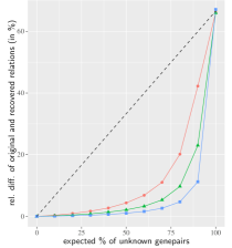
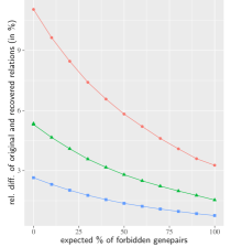
Figure 2: Shown are the average relative differences of original and recovered relations depending on the size of unknowns (left) and the size of additional forbidden relations (right).

Fig.  2(left) shows the average relative difference of the original full set $\mathcal{H}^{\star}(\mathcal{T})$ and the recovered full sets $\mathcal{H}^{\star}(\widetilde{\mathcal{T}})$ for each instance. The dashed line in the plots of Fig.  2(left) shows the expected relative difference when each unknown gene pair is assigned randomly to one of the relations in the partial set $\mathcal{H}$. As expected, the relative differences increases with the number of unassigned leaf pairs. Somewhat surprisingly, even if 80% of pairs of leaves are expected to be unassigned in $\mathcal{H}$, it is possible to averagely recover 79.8% - 95.3% of the original relations. Moreover, the plot in Fig. 2(left) also suggest that the accuracy of recovered homology relations increases with the input size, i.e., the number of leaves. To explain this fact, observe that the number of constraints given by the full set of homology relations on some leaf set $L$ is $O(|L|^{2})$. Conversely, the number of inner vertices in a tree only increases linearly with $L$, $O(|L|)$. Hence, on average the number of constraints given on the labeling of an internal vertex in the gene tree is $O(|L|^{2})/O(|L|)=O(|L|)$. Note, Alg. 1 constructs cotrees and hence, if there are more leaves, then there are also more constraints for the rules (labeling of the inner vertices) that are allowed to be applied. Therefore, with an increasing number of leaves the correct relation between unassigned pairs of leaves in $\mathcal{H}$ are already determined.

Fig.  2(right) shows the impact of additional forbidden relations for the instances where we have removed pairs $(x,y)$ with probability $p=0.7$. For each of the partial sets $\mathcal{H}$, we have chosen two vertices $x$ and $y$ where neither $(x,y)$ nor $(y,x)$ is contained in $\mathcal{H}$ with probability $p^{\prime}\in\{0.1,0.2,\dots,1\}$ and assigned $(x,y),(y,x)$ to a forbidden relation $F_{i}$ such that $(x,y),(y,x)\in R^{\star}_{j}(\mathcal{T})$ with $i,j\in\{0,1,\overrightarrow{1}\}$ implies that $i\neq j$. In other words, if $(x,y),(y,x)$ are assigned to $F_{i}$ with $i\in\{0,1,\overrightarrow{1}\}$ then $(x,y),(y,x)$ were not in the original set $R^{\star}_{j}(\mathcal{T})$. The latter is justified to ensure satisfiability of the partial relations w.r.t. the forbidden relations. Again, we compared the relative difference of the original full sets $\mathcal{H}^{\star}(\mathcal{T})$ and the recovered full sets $\mathcal{H}^{\star}(\widetilde{\mathcal{T}})$ computed with Alg.  1. The plot shows that, with an increasing number of forbidden leaf pairs, the relative difference decreases. Clearly, the more leaf pairs are forbidden the more of such leaf pairs are not allowed to be assigned to one of the relations. Therefore, the degree of freedom for assigning a relation to an unassigned pair decreases with an increase of the number of forbidden pairs.

One factor that may affect the results of the plots shown in Fig. 2 is the order in which rules are chosen when more than one rule is satisfied. By construction, Alg.  1 fixes the order of applied rules as follows: first Rule (1), then Rule (2), then Rule (3). In other words, when possible the trees for the satisfiable (strongly) connected components are first joined by a common root labeled “$1$”; if this does not apply, then with common root labeled “$0$”, and “$\overrightarrow{1}$” otherwise. To investigate this issue in more details, we modified Alg.  1 so that either a different fixed rule order or a random rule order is applied.

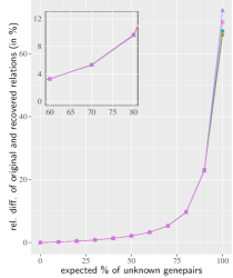
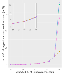
Figure 3: Shown are the average relative differences of original and recovered relations, depending on the percentage of unassigned pairs and the rule order for cotrees with uniform (left) and skewed (right) label distribution.

Fig.  3(left) shows the plot for the partial relations for the fixed leaf size $|L|=50$. The rule orders are shown in the legend of Fig.  3. Here, $X/Y/Z$, with $X,Y,Z\in\{1\ \widehat{=}\textrm{ Rule(2)},0\ \widehat{=}\textrm{ Rule(1)},\overrightarrow{1}\ \widehat{=}\textrm{ Rule(3)}\}$ being distinct; indicates that first rule $X$ is checked, then rule $Y$ and, if both are not applicable, then rule $Z$ is used. RAND means that each of the allowed rules are chosen with equal probability. As one can observe, the rule order does not have a significant impact on the quality of the recovered full sets. This observation might be explained by the fact that we have used a random assignment of events $0,1$ and $\overrightarrow{1}$ for the vertices of the initial simulated trees $T$.

To investigate this issue in more detail, we additionally used 1000 unlabeled simulated trees $T$ with $|L|=50$ and assigned to each vertex $v$ a label $t(v)=1$ with a probability $p=0.8$, label $t(v)=\overrightarrow{1}$ with $p=0.1$ and label $t(v)=0$ with $p=0.1$ Again, each resulting cotree $\mathcal{T}=(T;t)$ represents a full set $\mathcal{H}^{\star}(\mathcal{T})=\{R^{\star}_{0}(\mathcal{T}),R^{\star}_{1}(\mathcal{T}),R^{\star}_{\overrightarrow{1}}(\mathcal{T})\}$ from which we obtain partial sets $\mathcal{H}=\{R_{0},R_{1},R_{\overrightarrow{1}}\}$ as for the other instances. Fig.  3(right) shows the resulting plots. As it can be observed, even a quite skewed distribution of labels in the cotrees and the choice of rule order does not have an effect on the quality of the recovered full sets.

In summary, the results show that it suffices to have only a very few but correct pairs of the original relations to reconstruct most of them.

Appendix

Proof of Lemma 2

Proof

Assume that $\mathcal{H}$ is satisfiable w.r.t. $\mathcal{F}$. Hence, $\mathcal{H}$ can be extended to a full set $\mathcal{H}^{\star}=\{R^{\star}_{0},R^{\star}_{1},R^{\star}_{\overrightarrow{1}}\}$ that is satisfiable w.r.t. $\mathcal{F}$. Thus, there is a cotree $\mathcal{T}=({T},{t})$ that explains $\mathcal{\mathcal{H}^{\star}}$ and, in particular, $G^{\star}=(V,R^{\star}_{1}\cup R^{\star}_{\overrightarrow{1}})$ must be a di-cograph.

Let $\{C_{1},\dots,C_{k}\}$, $k\geq 1$ be a partition of $V$. Lemma 1 implies that $G^{\star}[C_{i}]$ is a di-cograph for any $i\in\{1,\dots,k\}$. Since $R^{\star}_{0}\cap F_{0}=R^{\star}_{1}\cap F_{1}=R^{\star}_{\overrightarrow{1}}\cap F_{\overrightarrow{1}}=\emptyset$, the di-cograph $G^{\star}$ as well as the relation $R^{\star}_{0}$ does not contain arcs in $F_{1},F_{0}$ and $F_{\overrightarrow{1}}$. Therefore, $G^{\star}[C_{i}]$ as well as the relation $R^{\star}_{0}[C_{i}]$ does not contain arcs in $F_{1},F_{0}$ and $F_{\overrightarrow{1}}$. This implies that the full set $\mathcal{H}^{\star}[C_{i}]$ restricted to the vertices in $C_{i}$ is satisfiable w.r.t. $\mathcal{F}[C_{i}]$. Hence, there is an extension $\mathcal{H}^{\star}[C_{i}]$ of the partial set $\mathcal{H}[C_{i}]$ that is satisfiable w.r.t. $\mathcal{F}[C_{i}]$ and therefore, $\mathcal{H}[C_{i}]$ is satisfiable w.r.t. $\mathcal{F}[C_{i}]$.

Now assume that for any partition $\{C_{1},\dots,C_{k}\}$ of $V$ the induced sub-relations in $\mathcal{H}[C_{i}]$ are satisfiable w.r.t. $\mathcal{F}[C_{i}]$. Thus, for the trivial partition $\{V\}$ of $V$, we have $\mathcal{H}[V]=\mathcal{H}$ is satisfiable w.r.t. $\mathcal{F}[V]=\mathcal{F}$, which completes the proof. ∎

Proof of Theorem 4.2

Proof

”$\Leftarrow$:” Assume that at least one of the conditions of Rule (0-3) is satisfied. We will show that one can extend $\mathcal{H}$ to a full set $\mathcal{H}^{\star}$ that is satisfiable w.r.t. $\mathcal{F}$.

Clearly, if Rule (0) is satisfied, then $\mathcal{H}$ is already full and the cotree that corresponds to the single-vertex graph $K_{1}$ explains $\mathcal{H}$. Hence, $\mathcal{H}$ is satisfiable w.r.t. $\mathcal{F}$. In what follows, we will therefore assume that $|V|\geq 2$.

Assume that Rule (1) is satisfied, and let $C_{1},\dots,C_{k}$, $k\geq 2$, be the connected components of $G_{0}$. Since $\mathcal{H}[C_{i}]$ is satisfiable w.r.t. $\mathcal{F}[C_{i}]$ for all $i\in\{1,\dots,k\}$, we can extend $\mathcal{H}[C_{i}]$ to a full set $\mathcal{H}^{\star}[C_{i}]$ that is satisfiable w.r.t. $\mathcal{F}[C_{i}]$. Hence, there exists a cotree $(T_{i},t_{i})$ representing $\mathcal{H}^{\star}[C_{i}]$. Let $\mathcal{H}^{\prime}=\{R^{\prime}_{0},R^{\star}_{1},R^{\star}_{\overrightarrow{1}}\}$ be the resulting partial set obtained from extending $\mathcal{H}$, such that $\mathcal{H}^{\star}[C_{i}]$ is full and satisfiable w.r.t. $\mathcal{F}[C_{i}]$ for all $i\in\{1,\dots,k\}$, and let $(T_{1},t_{1}),\dots,(T_{k},t_{k})$ be the cotrees explaining $\mathcal{H}^{\star}[C_{1}],\dots,\mathcal{H}^{\star}[C_{k}]$, respectively.

For any remaining unassigned pair $(x,y)\not\in R^{\prime}_{0}\cup R^{\star}_{1}\cup R_{\overrightarrow{1}}^{\star,sym}$, the vertices $x$ and $y$ must be contained in two distinct connected components $C_{i}$ and $C_{j}$ of $G_{0}$. Now, we extend $\mathcal{H^{\prime}}$ to a full set $\mathcal{H}^{\star}$ by adding all unassigned pairs to $R^{\prime}_{0}$ to obtain the set $R^{\star}_{0}$. We continue to show that $\mathcal{H}^{\star}=\{R^{\star}_{0},R^{\star}_{1},R^{\star}_{\overrightarrow{1}}\}$ is satisfiable w.r.t. $\mathcal{F}$. Let $x$ and $y$ be two vertices that reside in distinct connected components $C_{i}$ and $C_{j}$ of $G_{0}$. Clearly, $(x,y)\notin F_{0}\cup R_{1}\cup R_{\overrightarrow{1}}^{sym}$, as otherwise, $x$ and $y$ would be in the same connected component of $G_{0}$. By construction, $(x,y)\notin F_{0}\cup R^{\star}_{1}\cup R_{\overrightarrow{1}}^{\star,sym}$ and $F_{0}\cap R^{\star}_{0}=\emptyset$.

Now, we join cotrees $(T_{1},t_{1}),\dots,(T_{k},t_{k})$ the under a new root $\rho_{T}$ with label $0$ to obtain the cotree $(T,t)$. Note, any subtree rooted at a child of $\rho_{T}$ explains $\mathcal{H}^{\star}[C_{i}]$ for some connected component $C_{i}$ of $G_{0}$. Thus, $(x,y)\in R^{\star}_{0}$ if and only if $t(\operatorname{lca}(x,y))=0$. It follows that $(T,t)$ explains the full set $\mathcal{H}^{\star}=\{R^{\star}_{0},R^{\star}_{1},R^{\star}_{\overrightarrow{1}}\}$ and $R^{\star}_{0}\cap F_{0}=R^{\star}_{1}\cap F_{1}=R^{\star}_{\overrightarrow{1}}\cap F_{\overrightarrow{1}}=\emptyset$. Therefore $\mathcal{H}^{\star}$ is satisfiable w.r.t. $\mathcal{F}$. Hence, $\mathcal{H}$ is satisfiable w.r.t. $\mathcal{F}$.

The same arguments can be applied on the connected components of $G_{1}$ if Rule (2) is satisfied by extending every unassigned pair $x,y\in V$ between two distinct connected components of $G_{1}$ to $1$ and setting $t(\rho_{T})\coloneqq 1$. Again, $\mathcal{H}$ is satisfiable w.r.t. $\mathcal{F}$.

Finally, assume that Rule (3) is satisfied, and let $C_{1},\dots,C_{k}$, $k\geq 2$, be the strongly connected components of $G_{\overrightarrow{1}}$. As before, since $\mathcal{H}[C_{i}]$ is satisfiable w.r.t. $\mathcal{F}[C_{i}]$ for all $i\in\{1,\dots,k\}$, the induced subgraph $\mathcal{H}[C_{i}]$ can be extended to a full set that is satisfiable w.r.t. $\mathcal{F}[C_{i}]$. Again, we let $\mathcal{H}^{\prime}=\{R^{\star}_{0},R^{\star}_{1},R_{\overrightarrow{1}}^{\prime}\}$ be the resulting partial set obtained from $\mathcal{H}$, such that $\mathcal{H}^{\prime}[C_{i}]$ is a full satisfiable set w.r.t. $\mathcal{F}[C_{i}]$, for all $i\in\{1,\dots,k\}$. Let $(T_{1},t_{1}),\dots,(T_{k},t_{k})$ be the corresponding cotrees explaining $\mathcal{H}^{\prime}[C_{1}],\dots,\mathcal{H}^{\prime}[C_{k}]$, respectively. In what follows, we want to show that the cotree $(T,t)$ with root $\rho_{T}$ with $\overrightarrow{1}$ that is obtained by joining the cotrees $(T_{1},t_{1}),\dots(T_{k},t_{k})$ under the root $\rho_{T}$ in a particular order explains a full set $\mathcal{H}^{\star}=\{R^{\star}_{0},R^{\star}_{1},R^{\star}_{\overrightarrow{1}}\}$ that extends $\mathcal{H^{\prime}}$ and is satisfiable w.r.t.  $\mathcal{F}$. To this end, however, we need to investigate the structure of the relations $R_{0},R_{1},R_{\overrightarrow{1}}$ and $R^{\star}_{0},R^{\star}_{1},R_{\overrightarrow{1}}^{\prime}$ in some more detail.

Let $Q\coloneqq G_{\overrightarrow{1}}/\{C_{1},\dots,C_{k}\}$ be the quotient graph. By definition, $Q$ is a DAG, and thus, there exists a topological order $\pi$ on $Q$ such that for any arc $(C_{i},C_{j})\in E(Q)$, it holds that $\pi(C_{i})<\pi(C_{j})$. W.l.o.g. assume that $\pi$ is already given by the ordering of $C_{1},\dots,C_{k}$, i.e., $\pi(C_{i})\coloneqq i$ for all $i\in\{1,\dots,k\}$.

By construction, for any unassigned pair $(x,y)\not\in R^{\star}_{0}\cup R^{\star}_{1}\cup R^{\prime}_{\overrightarrow{1}}$ of $\mathcal{H}^{\prime}$, the two vertices $x$ and $y$ are contained in two distinct strongly connected components $C_{i}$ and $C_{j}$ of $G_{\overrightarrow{1}}$. Now, we extend $\mathcal{H}^{\prime}$ to a full set $\mathcal{H}^{\star}=\{R^{\star}_{0},R^{\star}_{1},R^{\star}_{\overrightarrow{1}}\}$, by adding all unassigned pairs $(x,y)$ with $x\in C_{i}$ and $y\in C_{j}$ to the relation $R^{\prime}_{\overrightarrow{1}}$ if and only if $i<j$, to obtain $R^{\star}_{\overrightarrow{1}}$.

Let $C_{i}$ and $C_{j}$ be distinct strongly connected components of $G_{\overrightarrow{1}}$. We show now that $(x,y)\in R^{\star}_{\overrightarrow{1}}$ for all $x\in C_{i}$ and $y\in C_{j}$ if and only if $i<j$. By construction, the latter is satisfied for all $(x,y)\in R^{\star}_{\overrightarrow{1}}\setminus R^{\prime}_{\overrightarrow{1}}$. Let $(u,v)$ be an already assigned pair that is contained in $R^{\star}_{0}\cup R^{\star}_{1}\cup R^{\prime}_{\overrightarrow{1}}$ such that $u\in C_{i}$ and $v\in C_{j}$. Therefore, $(x,y)\in R_{0}\cup R_{1}\cup R_{\overrightarrow{1}}$ since no pairs $(x,y)$ have been added between vertices $x\in C_{i}$ and $y\in C_{j}$ to obtain $R^{\star}_{0}\cup R^{\star}_{1}\cup R^{\prime}_{\overrightarrow{1}}$. But then, $(x,y)\in R_{\overrightarrow{1}}$, as otherwise symmetry of $R_{0}$ and $R_{1}$ would imply that $u$ and $v$ are in the same strongly connected component of $G_{\overrightarrow{1}}$. Furthermore, we added only pairs $(a,b)$ to $R_{\overrightarrow{1}}$ to obtain $R^{\prime}_{\overrightarrow{1}}$ where $a$ and $b$ are contained within the same strongly connected component of $G_{\overrightarrow{1}}$. Thus, for all $(u,v)\in R^{\star}_{0}\cup R^{\star}_{1}\cup R^{\prime}_{\overrightarrow{1}}$ with $u$ and $v$ in distinct strongly connected components $C_{1},\dots,C_{k}$ it holds that $(u,v)\in R_{\overrightarrow{1}}$. In summary, we added the unassigned pair $(x,y)$ with $x\in C_{i}$ and $y\in C_{j}$ to $R^{\prime}_{\overrightarrow{1}}$ if and only if $\pi(C_{i})=i<j=\pi(C_{j})$. In addition, any already assigned pair $(u,v)$ with $u\in C_{i}$ and $v\in C_{j}$ must be contained in $R_{\overrightarrow{1}}$, which implies that $(C_{i},C_{j})\in E(Q)$, and hence, $\pi(C_{i})=i<j=\pi(C_{j})$. Therefore, $(x,y)\in R^{\star}_{\overrightarrow{1}}$ if and only if $i<j$. Moreover, the latter arguments also ensure that the sets $R^{\star}_{0},R^{\star}_{1}$ and $R^{\star}_{\overrightarrow{1}}$ are pairwisely disjoint.

We continue to show that $R^{\star}_{\overrightarrow{1}}\cap F_{\overrightarrow{1}}=\emptyset$. By construction, $R^{\prime}_{\overrightarrow{1}}[C_{i}]$ is satisfiable w.r.t.  $F_{\overrightarrow{1}}[C_{i}]$ for all $i\in\{1,\dots,k\}$. Hence, $R^{\prime}_{\overrightarrow{1}}\cap F_{\overrightarrow{1}}=\emptyset$. Thus, it remains to show that for all $(x,y)\in R^{\star}_{\overrightarrow{1}}\setminus R^{\prime}_{\overrightarrow{1}}$ it holds that $(x,y)\not\in F_{\overrightarrow{1}}$. Let $(x,y)\in R^{\star}_{\overrightarrow{1}}\setminus R^{\prime}_{\overrightarrow{1}}$. Thus, $x\in C_{i}$ and $y\in C_{j}$ for some strongly connected components of $G_{\overrightarrow{1}}$ with $i<j$. Since $(x,y)\notin R^{\prime}_{\overrightarrow{1}}$, we also have $(x,y)\not\in R_{\overrightarrow{1}}$. Assume for contraction that $(x,y)\in F_{\overrightarrow{1}}$. Hence, $(y,x)\in\overleftarrow{F_{\overrightarrow{1}}}$. However, this would imply that $(C_{j},C_{i})\in E(Q)$, meaning that $i>j$ and therefore $(x,y)\not\in R^{\star}_{\overrightarrow{1}}$; a contradiction.

We are now in the position to create a cotree $(T,t)$ that explains $\mathcal{H}^{\star}=\{R^{\star}_{0},R^{\star}_{1},R^{\star}_{\overrightarrow{1}}\}$. To this end, we join the cotrees $(T_{1},t_{1}),\dots(T_{k},t_{k})$ under common root $\rho_{T}$ with label $\overrightarrow{1}$. Moreover, cotrees $(T_{1},t_{1}),\dots(T_{k},t_{k})$ are added to $(T,t)$ such that any leaf of $T_{i}$ is left of any leaf of $T_{j}$ iff $i<j$. By construction $(T,t)$ explains all sub-relations in $\mathcal{H}^{\star}[C_{i}]$, $1\leq i\leq k$. For any other pair $(x,y)$ where $x$ and $y$ are contained in different strongly connected components $C_{i}$ and $C_{j}$ of $G_{\overrightarrow{1}}$, respectively, we have $(x,y)\in R^{\star}_{\overrightarrow{1}}$, $(y,x)\not\in R^{\star}_{\overrightarrow{1}}$, $(x,y)\not\in F_{\overrightarrow{1}}$ and $i<j$. As shown above, $R^{\star}_{0}\cap F_{0}=R^{\star}_{1}\cap F_{1}=R^{\star}_{\overrightarrow{1}}\cap F_{\overrightarrow{1}}=\emptyset$. By construction, $t(\operatorname{lca}_{T}(x,y))=t(\rho_{T})=\overrightarrow{1}$ and $x$ is placed left of $y$ in $T$. Therefore, any pair $(x,y)\in R^{\star}_{\overrightarrow{1}}$ is explained by $(T,t)$. In summary, $(T,t)$ explains $\mathcal{H}^{\star}$ and $\mathcal{H}^{\star}$ is satisfiable w.r.t. $\mathcal{F}$. Hence, $\mathcal{H}$ is satisfiable w.r.t. $\mathcal{F}$.

“$\Rightarrow:$” Assume that $\mathcal{H}=\{R_{0},R_{1},R_{\overrightarrow{1}}\}$ is satisfiable w.r.t. $\mathcal{F}$. Trivially, Rule (0) is satisfied in the case that $|V|=1$. Hence, let $|V|\geq 2$. By assumption, $R_{0},R_{1}$ and $R_{\overrightarrow{1}}$ can be extended to obtain a full satisfiable set $\mathcal{H}^{\star}=\{R^{\star}_{0},R^{\star}_{1},R^{\star}_{\overrightarrow{1}}\}$ such that $R^{\star}_{0}\cap F_{0}=R^{\star}_{1}\cap F_{1}=R^{\star}_{\overrightarrow{1}}\cap F_{\overrightarrow{1}}=\emptyset$. Hence, there is a cotree $(T;t)$ that explains $\mathcal{H}^{\star}$. Consider the root $\rho_{T}$ of $T$ with children $v_{1},\dots,v_{k}$ and the particular leaf sets $L(v_{1}),\dots,L(v_{k})$. Note that, by definition of cotrees each inner vertex of $(T;t)$, and in particular the root $\rho_{T}$ has at least two children.

Assume that $\rho_{T}$ is labeled $0$. Since $(T;t)$ explains $\mathcal{H}^{\star}$, for any $x\in L(v_{i})$ and $y\in L(v_{j})$, $i\neq j$ we have $(x,y),(y,x)\in R^{\star}_{0}$. Since additionally $R^{\star}_{0}\cap F_{0}=\emptyset$, the digraph $G^{\star}_{0}\coloneqq(V,R^{\star}_{1}\cup R^{\star}_{\overrightarrow{1}}\cup F_{0})$ must be disconnected. Since $G_{0}$ is a subgraph of $G^{\star}_{0}$, the graph $G_{0}$ is disconnected as well. By Lemma 2, $\mathcal{H}[C]$ is satisfiable w.r.t. $\mathcal{F}[C]$ for any connected components $C$ of $G_{0}$. Hence, Rule (1) is satisfied.

If $\rho_{T}$ is labeled $1$, then we can apply analogous arguments to see that $G^{\star}_{1}$ and $G_{1}$ are disconnected and that Rule (2) is satisfied.

Now assume that $\rho_{T}$ is labeled $\overrightarrow{1}$. Let $x\in L(v_{i})$ and $y\in L(v_{j})$, $i\neq j$ and assume that $x$ is placed left of $y$ in $T$. Since $(T,t)$ explains $\mathcal{H}^{\star}$, we have $(x,y)\in R^{\star}_{\overrightarrow{1}}$ and $(y,x)\notin R^{\star}_{\overrightarrow{1}}$. Moreover, $(x,y)\in R^{\star}_{\overrightarrow{1}}$ implies that $(x,y)\notin F_{\overrightarrow{1}}$ and thus, $(y,x)\notin\overleftarrow{F_{\overrightarrow{1}}}$. The latter together with the disjointedness of the sets $R^{\star}_{0},R^{\star}_{1},R^{\star}_{\overrightarrow{1}}$ implies that $(x,y)\in E(G^{\star}_{\overrightarrow{1}})$ and $(y,x)\notin E(G^{\star}_{\overrightarrow{1}})$, where $G^{\star}_{\overrightarrow{1}}\coloneqq(V,R^{\star}_{0}\cup R^{\star}_{1}\cup R^{\star}_{\overrightarrow{1}}\cup\overleftarrow{F_{\overrightarrow{1}}})$. Since the latter is satisfied for all elements in any of the leaf sets $L(v_{1}),\dots,L(v_{k})$, we immediately obtain that $G^{\star}_{\overrightarrow{1}}=G^{\star}_{\overrightarrow{1}}[L(v_{1})]\oslash\dots\oslash G^{\star}_{\overrightarrow{1}}[L(v_{k})]$. Hence, $G^{\star}_{\overrightarrow{1}}$ contains more than one strongly connected component. Since $G_{\overrightarrow{1}}$ is a subgraph of $G^{\star}_{\overrightarrow{1}}$, it follows that $G_{\overrightarrow{1}}$ contains more than one strongly connected component. By Lemma 2, $\mathcal{H}[C]$ is satisfiable w.r.t. $\mathcal{F}[C]$ for all strongly connected components $C$ of $G_{\overrightarrow{1}}$. Hence, Rule (3) is satisfied. ∎

Correctness of Recognition Algorithm 1

In this part we provide a polynomial-time algorithm for the recognition of partial satisfiable sets $\mathcal{H}$ and the reconstruction of respective extended sets $\mathcal{H}^{\star}$ and a cotree $(T,t)$ that explains $\mathcal{H}$, in case $\mathcal{H}$ is satisfiable. Thm.  4.2 gives a characterization of satisfiable partial sets with respect to some forbidden set. However, in order to design a polynomial-time algorithm, we have to decide which rule can be applied at which step. Note, several rules might be fulfilled at the same time, that is, the graph $G_{0}$ and $G_{1}$ can be disconnected and $G_{\overrightarrow{1}}$ can contain more than one strongly connected component at the same time. Since sub-condition (b) for each Rule (1-3) is recursively defined, we might end in a non-polynomial algorithm, if a “correct” choice of the rule would be important. A trivial example where all rules can be applied at the same time is given by the partial set of empty relations $\mathcal{H}=\{\emptyset,\emptyset,\emptyset\}$. Interestingly, Lemma 2 immediately implies that it does not matter which applicable rule is chosen to obtain $\mathcal{H}^{\star}$ that is satisfiable w.r.t. $\mathcal{F}$.

Corollary 3

Let $\mathcal{H}=\{R_{0},R_{1},R_{\overrightarrow{1}}\}$ be a partial set, and $\mathcal{F}=\{F_{0},F_{1},F_{\overrightarrow{1}}\}$ a forbidden set. Assume that Rule (i).a and (j).a with $i,j\in\{1,2,3\}$ (as given in Thm. 4.2) are satisfied.

Then, $\mathcal{H}$ is satisfiable w.r.t. $\mathcal{F}$ if and only if Rule i.b and j.b are satisfied.

Thm.  4.2 together with Corollary 3 immediately yields a polynomial time recursive algorithm to determine satisfiability of a homology set with respect to a forbidden set. Moreover, if $\mathcal{H}$ is satisfiable w.r.t $\mathcal{F}$ the proof of Thm.  4.2 describes how to construct a cotree explaining a full satisfiable set w.r.t $\mathcal{F}$ extended from $\mathcal{H}$. The algorithm is summarized in Alg.  1.

See 4.3

Proof

The correctness of Alg.  1 follows from Thm.  4.2 and Corollary 3. To be more precise, Alg. 1 checks whether condition Rule (0) or Rule (1-3)(a), as defined in Thm.  4.2, is satisfied.

As a preprocessing step, the algorithm first checks if $R_{0}\cap F_{0}=R_{1}\cap F_{1}=R_{\overrightarrow{1}}\cap F_{\overrightarrow{1}}=\emptyset$ (Line 3). If this is not the case, clearly $\mathcal{H}$ cannot be satisfiable w.r.t. $\mathcal{F}$, and hence the algorithm stops. If no forbidden pairs are present in $\mathcal{H}$, we will try and build the cotree explaining a full set, extended from $\mathcal{H}$, that is satisfiable w.r.t. $\mathcal{F}$. Note, Corollary 3 implies that the order of applied rules does not matter.

If Rule (0) is satisfied, i.e., $|V|=1$, then $\mathcal{H}$ is already full and satisfiable w.r.t. $\mathcal{F}$, and $(T;t)=((V,\emptyset);\emptyset)$ is a valid cotree explaining $\mathcal{H}$, and thus returned on Line 7.

If Rule (1a) (resp. (2a)) is satisfied (Line 8), then Alg.  1 is called recursively on each of the connected components defined by $G_{0}$ ($G_{1}$ resp.) to verify that Rule (1b) (resp. (2b)) is satisfied. If the connected components are indeed satisfiable, the obtained cotrees are joined into a single cotree explaining a full set $\mathcal{H}^{\star}$ that is satisfiable w.r.t. $\mathcal{F}$ as described in the proof of Thm.  4.2. This set $\mathcal{H}^{\star}$ is an extension of $\mathcal{H}$. The resulting cotree is then returned.

If Rule (3a) is satisfied (Line 12), Alg.  1 is then called recursively to verify whether Rule (3b) is satisfied, and if so, the obtained cotrees are joined into a single cotree $(T;t)$. Note, $Q\coloneqq G_{\overrightarrow{1}}/\{C_{1},\dots,C_{k}\}$ is a DAG and there exists a topological order $\pi$ on $Q$. The cotrees are joined to obtain cotree $(T;t)$ from left to right such that ordering $\pi$ is preserved, as in the construction described in the proof of Thm.  4.2. Thus, we obtain a cotree $(T,t)$ that explains a full set $\mathcal{H}^{\star}$ that is satisfiable w.r.t. $\mathcal{F}$ and an extension of $\mathcal{H}$. Finally, $(T;t)$ is returned.

If neither of the rules are satisfied, Thm.  4.2 implies that $\mathcal{H}$ is not satisfiable w.r.t. $\mathcal{F}$ and the algorithm stops. Hence, a cotree is returned that explains the partial set $\mathcal{H}$ if and only if $\mathcal{H}$ is satisfiable w.r.t. $\mathcal{F}$.

For the runtime, observe first that $R_{0}\cap F_{0}=R_{1}\cap F_{1}=R_{\overrightarrow{1}}\cap F_{\overrightarrow{1}}$ (Line 3) can be computed in $O(m)$ time. Moreover, all digraphs defined in Rule (1-3) of Thm.  4.2, can be constructed in $O(n+m)$ time. Furthermore, each of the following tasks can be performed in $O(n+m)$ time: finding the (strongly) connected components of each digraph, building the defined quotient graph, and finding the topological order on the quotient graph. Similarly, constructing $V[C_{i}]$, $\mathcal{H}[C_{i}]$, and $\mathcal{F}[C_{i}]$ (Line 10, 15) for each (strongly) connected component, can also be done in $O(n+m)$ time for all components, by going through every element in $V$, $\mathcal{H}$, and $\mathcal{F}$ and assigning each pair to their respective induced subset.

Thus, every pass of BuildCotree takes $O(n+m)$ time. Since every call to BuildCotree adds a vertex to the final constructed cotree, and the number of vertices in a tree is bounded by the number $n$ of leaves, it follows that BuildCotree can be called at most $O(n)$ times. Therefore, we end in an overall running time of $O(m+n(n+m))=O(n^{2}+nm)$ for Alg.  1. ∎

Alg.  1 provides a cotree, $(T;t)$, explaining a full satisfiable set, $\mathcal{H}^{\star}=\{R^{\star}_{0},R^{\star}_{1},R^{\star}_{\overrightarrow{1}}\}$, extended from a given partial set $\mathcal{H}$, such that $\mathcal{H}^{\star}$ is satisfiable w.r.t. a forbidden set $\mathcal{F}$. The algorithm however, does not directly output $\mathcal{H}^{\star}$. Nevertheless, $\mathcal{H}^{\star}$ can easily be constructed given $(T;t)$:

Theorem 5.1

Let $\mathcal{H}=\{R_{0},R_{1},R_{\overrightarrow{1}}\}$ be a partial set that is satisfiable w.r.t a forbidden set $\mathcal{F}=\{F_{0},F_{1},F_{\overrightarrow{1}}\}$ and $(T,t)$ be a cotree that explains $\mathcal{H}$. Then, a full satisfiable homology set $\mathcal{H}^{\star}=\{R^{\star}_{0},R^{\star}_{1},R^{\star}_{\overrightarrow{1}}\}$ that extends $\mathcal{H}$ can be constructed in $O(|V|^{2})$ time.

Proof

To recap, the leaf set of $(T=(W,E);t)$ is $L(T)=V$. The full set $\mathcal{H}^{\star}$ can be obtained from $(T;t)$ as follows: For every two leaves $x,y\in V$, where $x$ is left of $y$ in $T$ and $(x,y)\not\in R_{0}\cup R_{1}\cup{R_{\overrightarrow{1}}^{sym}}$, we add the unassigned pair $(x,y)$ to $R_{0}$, $R_{1}$, or $R_{\overrightarrow{1}}$ depending on whether $t(\operatorname{lca}(x,y))$ equals $0$, $1$, or $\overrightarrow{1}$ respectively. If $(x,y)$ was added to $R_{0}$ (resp. $R_{1}$), then we also add $(y,x)$ to $R_{0}$ (resp. $R_{1}$). Since we address all two leaves $x,y\in V$, we obtain $R^{\star}_{0}=R_{0}({\mathcal{T}})$, $R^{\star}_{1}=R_{1}({\mathcal{T}})$, and $R^{\star}_{\overrightarrow{1}}=R_{\overrightarrow{1}}({\mathcal{T}})$. Hence, the resulting set $\mathcal{H}^{\star}$ is full and explained by $(T;t)$.

It was shown in [31], that the lowest common ancestor, $\operatorname{lca}(x,y)$, can be accessed in constant time, after an $O(|W|)$ preprocessing step. Since we look up the label $t(\operatorname{lca}(x,y))$ for each pair of leaves in $T$, it follows that $\mathcal{H}^{\star}$ can be constructed in $O(|L(T)|^{2})=O(|V|^{2})$ time. Hence, $\mathcal{H}^{\star}$ can be constructed from $(T,t)$ in $O(n^{2})$. ∎

The relative difference of original and recovered full sets

The relative difference between the true full set $\mathcal{H}^{\star}$ on $V^{\times}_{\mathrm{irr}}$ and the respective recovered full set $\mathcal{H}^{\prime}$ is given by

$$\frac{|R^{\star}_{0}\Delta R_{0}^{\prime}|+|R^{\star}_{1}\Delta R_{1}^{\prime}|+2|R^{\star}_{\overrightarrow{1}}\cap\overleftarrow{R^{\prime}_{\overrightarrow{1}}}|+2|(R^{\star}_{\overrightarrow{1}}\setminus\overleftarrow{R^{\prime}_{\overrightarrow{1}}})\Delta R_{\overrightarrow{1}}^{\prime}|}{|L|^{2}-|L|},$$

where $\Delta$ denotes the symmetric set difference.

Here, the term $|L|^{2}-|L|$ gives the number of all possible elements in a symmetric and irreflexive relation on $L$. Thus, the terms $|R^{\star}_{0}\Delta R_{0}^{\prime}|/(|L|^{2}-|L|)$ and $|R^{\star}_{1}\Delta R_{1}^{\prime}|/(|L|^{2}-|L|)$ gives the relative difference for the symmetric relations $R^{\star}_{0},R_{0}^{\prime}$ and $R^{\star}_{1},R_{1}^{\prime}$, respectively. For the term $f=2|R^{\star}_{\overrightarrow{1}}\cap\overleftarrow{R^{\prime}_{\overrightarrow{1}}}|/(|L|^{2}-|L|)$, recall that $R^{\star}_{\overrightarrow{1}}$ and $R_{\overrightarrow{1}}^{\prime}$ are anti-symmetric relations and observe that $(x,y)\in R^{\star}_{\overrightarrow{1}},(y,x)\in R_{\overrightarrow{1}}^{\prime}$ implies that $(x,y)\in R^{\star}_{\overrightarrow{1}}\cap\overleftarrow{R^{\prime}_{\overrightarrow{1}}}$. The term $\frac{1}{2}(|L|^{2}-|L|)$ gives the number of all possible elements in an anti-symmetric irreflexive relation on $L$. Hence, to count the relative differences of these sets we have to add the term $f$. Furthermore, $(R^{\star}_{\overrightarrow{1}}\setminus\overleftarrow{R^{\prime}_{\overrightarrow{1}}})\Delta R_{\overrightarrow{1}}^{\prime}$ contains all pairs $(x,y)\in R^{\star}_{\overrightarrow{1}}$ for which there is no pair on $x$ and $y$ contained in $R_{\overrightarrow{1}}^{\prime}$, or vice versa. By similar arguments as before, we finally have to add the term $2|(R^{\star}_{\overrightarrow{1}}\setminus\overleftarrow{R^{\prime}_{\overrightarrow{1}}})\Delta R_{\overrightarrow{1}}^{\prime}|/(|L|^{2}-|L|)$.

References

- [1] Altenhoff, A.M., Dessimoz, C.: Phylogenetic and functional assessment of orthologs inference projects and methods. PLoS Comput Biol. 5, e1000262 (2009)
- [2] Altenhoff, A.M., Gil, M., Gonnet, G.H., Dessimoz, C.: Inferring hierarchical orthologous groups from orthologous gene pairs. PLoS ONE 8(1), e53786 (2013)
- [3] Altenhoff, A.M., Škunca, N., Glover, N., Train, C.M., Sueki, A., Piližota, I., Gori, K., Tomiczek, B., Müller, S., Redestig, H., Gonnet, G.H., Dessimoz, C.: The OMA orthology database in 2015: function predictions, better plant support, synteny view and other improvements. Nucleic Acids Res 43(D1), D240–D249 (2015)
- [4] Böcker, S., Dress, A.W.M.: Recovering symbolically dated, rooted trees from symbolic ultrametrics. Adv. Math. 138, 105–125 (1998)
- [5] Brandstädt, A., Le, V.B., Spinrad, J.P.: Graph Classes: A Survey. Society for Industrial and Applied Mathematics, Philadelphia, PA, USA (1999)
- [6] Chen, F., Mackey, A.J., Stoeckert, C.J., Roos, D.S.: OrthoMCL-db: querying a comprehensive multi-species collection of ortholog groups. Nucleic Acids Res 34(S1), D363–D368 (2006)
- [7] Corneil, D.G., Lerchs, H., Steward Burlingham, L.: Complement reducible graphs. Discr. Appl. Math. 3, 163–174 (1981)
- [8] Corneil, D.G., Perl, Y., Stewart, L.K.: A linear recognition algorithm for cographs. SIAM J. Computing 14, 926–934 (1985)
- [9] Crespelle, C., Paul, C.: Fully dynamic recognition algorithm and certificate for directed cographs. Discr. Appl. Math. 154, 1722–1741 (2006)
- [10] Dessimoz, C., Margadant, D., Gonnet, G.H.: DLIGHT – lateral gene transfer detection using pairwise evolutionary distances in a statistical framework. In: Proceedings RECOMB 2008. pp. 315–330. Springer, Berlin, Heidelberg (2008)
- [11] Dondi, R., El-Mabrouk, N., Lafond, M.: Correction of weighted orthology and paralogy relations-complexity and algorithmic results. In: International Workshop on Algorithms in Bioinformatics. pp. 121–136. Springer (2016)
- [12] Engelfriet, J., Harju, T., Proskurowski, A., Rozenberg, G.: Characterization and complexity of uniformly nonprimitive labeled 2-structures. Theor. Comp. Sci. 154, 247–282 (1996)
- [13] Fitch, W.M.: Homology: a personal view on some of the problems. Trends Genet. 16, 227–231 (2000)
- [14] Gao, Y., Hare, D.R., Nastos, J.: The cluster deletion problem for cographs. Discrete Mathematics 313(23), 2763 – 2771 (2013)
- [15] Gurski, F.: Dynamic programming algorithms on directed cographs. Statistics, Optimization & Information Computing 5(1), 35–44 (2017)
- [16] Hartmann, K., Wong, D., Stadler, T.: Sampling trees from evolutionary models. Systematic biology 59(4), 465–476 (2010)
- [17] Hellmuth, M., Hernandez-Rosales, M., Huber, K.T., Moulton, V., Stadler, P.F., Wieseke, N.: Orthology relations, symbolic ultrametrics, and cographs. J. Math. Biology 66(1-2), 399–420 (2013)
- [18] Hellmuth, M., Stadler, P.F., Wieseke, N.: The mathematics of xenology: Di-cographs, symbolic ultrametrics, 2-structures and tree- representable systems of binary relations. Journal of Mathematical Biology 75(1), 199–237 (2017)
- [19] Hellmuth, M., Wieseke, N.: From sequence data including orthologs, paralogs, and xenologs to gene and species trees. In: Pontarotti, P. (ed.) Evolutionary Biology: Convergent Evolution, Evolution of Complex Traits, Concepts and Methods. pp. 373–392. Springer, Cham (2016)
- [20] Hellmuth, M., Wieseke, N., Lechner, M., Lenhof, H.P., Middendorf, M., Stadler, P.F.: Phylogenomics with paralogs. Proceedings of the National Academy of Sciences 112(7), 2058–2063 (2015)
- [21] Lafond, M., Dondi, R., El-Mabrouk, N.: The link between orthology relations and gene trees: a correction perspective. Algorithms for Molecular Biology 11(1), 1 (2016)
- [22] Lafond, M., El-Mabrouk, N.: Orthology and paralogy constraints: satisfiability and consistency. BMC Genomics 15(6), S12 (2014)
- [23] Lafond, M., El-Mabrouk, N.: Orthology relation and gene tree correction: complexity results. In: International Workshop on Algorithms in Bioinformatics. pp. 66–79. Springer (2015)
- [24] Lawrence, J.G., Hartl, D.L.: Inference of horizontal genetic transfer from molecular data: an approach using the bootstrap. Genetics 131(3), 753–760 (1992)
- [25] Lechner, M., Findeiß, S., Steiner, L., Marz, M., Stadler, P.F., Prohaska, S.J.: Proteinortho: detection of (co-)orthologs in large-scale analysis. BMC Bioinformatics 12, 124 (2011)
- [26] Lechner, M., Hernandez-Rosales, M., Doerr, D., Wiesecke, N., Thevenin, A., Stoye, J., Hartmann, R.K., Prohaska, S.J., Stadler, P.F.: Orthology detection combining clustering and synteny for very large datasets. PLoS ONE 9(8), e105015 (08 2014)
- [27] Liu, Y., Wang, J., Guo, J., Chen, J.: Complexity and parameterized algorithms for cograph editing. Theoretical Computer Science 461(0), 45 – 54 (2012)
- [28] McConnell, R.M., De Montgolfier, F.: Linear-time modular decomposition of directed graphs. Discrete Applied Mathematics 145(2), 198–209 (2005)
- [29] Östlund, G., Schmitt, T., Forslund, K., Köstler, T., Messina, D.N., Roopra, S., Frings, O., Sonnhammer, E.L.: InParanoid 7: new algorithms and tools for eukaryotic orthology analysis. Nucleic acids research 38(suppl 1), D196–D203 (2010)
- [30] Ravenhall, M., Škunca, N., Lassalle, F., Dessimoz, C.: Inferring horizontal gene transfer. PLoS Comput Biol 11(5), e1004095 (2015)
- [31] Schieber, B., Vishkin, U.: On finding lowest common ancestors: Simplification and parallelization. SIAM Journal on Computing 17(6), 1253–1262 (1988)
- [32] Sukumaran, J., Holder, M.T.: Dendropy: a python library for phylogenetic computing. Bioinformatics 26(12), 1569–1571 (2010)
- [33] Tatusov, R.L., Galperin, M.Y., Natale, D.A., Koonin, E.V.: The COG database: a tool for genome-scale analysis of protein functions and evolution. Nucleic Acids Research 28(1), 33–36 (2000)
- [34] Trachana, K., Larsson, T.A., Powell, S., Chen, W.H., Doerks, T., Muller, J., Bork, P.: Orthology prediction methods: A quality assessment using curated protein families. BioEssays 33(10), 769–780 (2011)