Perturbative Renormalization of Wilson line operators

Abstract

We present results for the renormalization of gauge invariant nonlocal fermion operators which contain a Wilson line, to one loop level in lattice perturbation theory. Our calculations have been performed for Wilson/clover fermions and a wide class of Symanzik improved gluon actions. The extended nature of such ‘long-link’ operators results in a nontrivial renormalization, including contributions which diverge linearly as well as logarithmically with the lattice spacing, along with additional finite factors. We present nonperturbative prescriptions to extract the linearly divergent contributions.

1 Introduction

Parton distribution functions (PDFs) provide important information on the quark and gluon structure of hadrons; at leading twist, they give the probability of finding a specific parton in the hadron carrying certain momentum and spin, in the infinite momentum frame. Due to the fact that PDFs are light-cone correlation functions, they cannot be computed directly on a Euclidean lattice. Nevertheless, there is an alternative approach, proposed by X. Ji, involving the computation of quasi-distribution functions, which are accessible in Lattice QCD. Exploratory studies of the quasi-PDFs reveal promising results for the non-singlet operators in the unpolarized, helicity and transversity cases.

A standard way of extracting quasi-distribution functions in lattice simulations involves computing hadronic matrix elements of certain gauge-invariant nonlocal operators; these are made up of a product of an anti-quark field at position $x$, possibly some Dirac gamma matrices, a path-ordered exponential of the gauge field (Wilson line) along a path joining points $x$ and $y$, and a quark field at position $y$. Given the extended nature of such operators, an endless variety of them, with different quantum numbers, can be defined and studied in lattice simulations and in phenomenological models. In pure gauge theories, prototype nonlocal operators are path-ordered exponentials along closed contours (Wilson loops); the contours may be smooth, but they may also contain angular points (cusps) and self-intersections.

The history of investigations of nonlocal operators in gauge theories goes back a long time. In particular, the renormalization of Wilson loops has been studied perturbatively, in dimensional regularization (DR). Using arguments valid to all orders in perturbation theory, it was shown that smooth Wilson loops in DR are finite functions of the renormalized coupling, while the presence of cusps and self-intersections introduces logarithmically divergent multiplicative renormalization factors; at the same time, it was shown that other regularization schemes are expected to lead to further renormalization factors $Z$ which are linearly divergent with the dimensionful ultraviolet cutoff $a$:

$$Z=e^{\displaystyle-c\,L/a}\,,$$ (1)

where $c$ is a dimensionless function of the renormalized coupling $g$, and $L$ is the loop length.

There are several obstacles which need to be overcome before a transparent picture of PDFs can emerge via Ji’s approach; one such obstacle is clearly the intricate renormalization behavior, which is the object of our present study. In what follows we formulate the problem, providing the definitions for the operators which we set out to renormalize, along with the renormalization prescription. Our calculations are performed both in dimensional regularization and on the lattice; we address in detail new features appearing on the lattice, such as contributions which diverge linearly and logarithmically with the lattice spacing, and finite mixing effects allowed by hypercubic symmetry. We also provide a prescription for estimating the linear divergence using non-perturbative data and extending arguments from perturbation theory. Finally, we point out some open questions for future investigations. A long write-up of our work, together with an extended list of references, can be found in Constantinou:2017sej (see also the companion paper Alexandrou:2017huk ).

2 Formulation

In our lattice calculations we make use of the clover (Sheikholeslami-Wohlert) fermion action; we allow the clover parameter, $c_{\rm SW}$, to be free throughout. We are interested in mass-independent renormalization schemes, and therefore we set the Lagrangian masses for each flavor, $m^{f}_{0}$ , to their critical value; for a one-loop calculation this corresponds to $m^{f}_{0}{=}0$. In the gluon sector we employ a 3-parameter family of Symanzik-improved actions involving Wilson loops with 4 and 6 links; members of this family are the Wilson, Iwasaki and tree-level Symanzik-improved actions.

The operators which we study in this work have the general form:

$$\mathcal{O}_{\Gamma}\equiv\overline{\psi}(x)\,\Gamma\,\mathcal{P}\,e^{i\,g\,\int_{0}^{z}A^{\mu}(x+\zeta\hat{\mu})d\zeta}\,\psi(x+z\hat{\mu})\,,$$ (2)

with a Wilson line of length $z$ inserted between the fermion fields in order to ensure gauge invariance. The appearance of contact terms beyond tree level renders the limit $z\to 0$ nonanalytic. We consider only cases where the Wilson line is a straight line along the $\mu$-axis. Without loss of generality we choose $\mu=1$. We perform our calculation for all independent combinations of Dirac matrices, $\Gamma$, that is:

$$\Gamma=\hat{1},\quad\gamma^{5},\quad\gamma^{\nu},\quad\gamma^{5}\,\gamma^{\nu},\quad\sigma^{\nu\rho}.$$ (3)

In the above, $\rho\neq\mu$ and we distinguish between the cases in which the index $\nu$ is in the same direction as the Wilson line ($\nu=\mu$), or perpendicular to the Wilson line ($\nu\neq\mu$). The 16 possible choices of $\Gamma$ are separated into 8 subgroups, whose renormalization is a priori different, defined as follows:

$$\begin{array}[]{lcllcllcllclrcl}{S}&\equiv&\mathcal{O}_{\hat{1}}&{V}_{1}&\equiv&\mathcal{O}_{\gamma^{1}}&{V}_{\nu}&\equiv&\mathcal{O}_{\gamma^{\nu}}&{T}_{1\nu}&\equiv&\mathcal{O}_{\sigma^{1\nu}}&(\nu,\rho&=&2,3,4)\\ {P}&\equiv&\mathcal{O}_{\gamma^{5}}&{A}_{1}&\equiv&\mathcal{O}_{\gamma^{5}\gamma^{1}}&{A}_{\nu}&\equiv&\mathcal{O}_{\gamma^{5}\gamma^{\nu}}&{T}_{\nu\rho}&\equiv&\mathcal{O}_{\sigma^{\nu\rho}}\,.\end{array}$$ (4)

We perform the calculation in both dimensional (DR) and lattice (LR) regularizations, which allows one to extract the lattice renormalization functions directly in the continuum ${\overline{\rm MS}}$-scheme.

In the LR calculation we encounter finite mixing for some pairs of operators (see Subsection 3.2), and, thus, here we provide the renormalization prescription in the presence of mixing between two structures, $\Gamma_{1}$ and $\Gamma_{2}$, where one has, a $2\times 2$ mixing matrix ($Z$). More precisely, we find mixing within each of the pairs: $\{S,\,V_{1}\}$, $\{A_{2},\,T_{34}\}$, $\{A_{3},\,T_{42}\}$, $\{A_{4},\,T_{23}\}$, in the lattice regularization. In these cases, the renormalization of the operators is then given by a set of 2 equations:

$$\binom{{\cal O}_{\Gamma_{1}}^{R}}{{\cal O}_{\Gamma_{2}}^{R}}=\begin{pmatrix}Z_{11}&Z_{12}\\ Z_{21}&Z_{22}\end{pmatrix}^{-1}\binom{{\cal O}_{\Gamma_{1}}}{{\cal O}_{\Gamma_{2}}}\,.$$ (5)

Once the mixing matrix $Z_{ij}$ is obtained through the perturbative calculation of certain amputated Green’s functions, as shown below, it can be applied to non-perturbative bare Green’s functions derived from lattice simulation data, in order to deduce the renormalized, disentangled Green’s functions for each of the two operators separately Alexandrou:2017huk .

The one-loop renormalized Green’s function of operator $\mathcal{O}_{\Gamma_{i}}$ can be obtained from the one-loop bare Green’s function of $\mathcal{O}_{\Gamma_{i}}$ and the tree-level Green’s function of $\mathcal{O}_{\Gamma_{j}}$ ($j\neq i$); this can be seen starting from the general expression:

$$\langle\psi^{R}\,{\cal O}^{R}_{\Gamma_{i}}\,\bar{\psi}^{R}\rangle=Z_{\psi}\,\sum_{j=1}^{2}\,(Z^{-1})_{ij}\,\langle\psi\,{\mathcal{O}}_{\Gamma_{j}}\,\bar{\psi}\rangle\,,\qquad\psi=Z^{1/2}_{\psi}\psi^{R}\,,$$ (6)

where the matrix $Z$ and the fermion field renormalization $Z_{\psi}$ have the following expansion:

$$Z_{ij}=\delta_{ij}+g^{2}z_{ij}+\mathcal{O}(g^{4})\,,\qquad Z_{\psi}=1+g^{2}z_{\psi}+\mathcal{O}(g^{4})\,.$$ (7)

Once the ${\overline{\rm MS}}$ Green’s functions have been computed in DR, the condition for extracting $Z^{LR,\,{\overline{\rm MS}}}_{ij}$ is simply the requirement that renormalized Green’s functions be regularization independent:

$$\langle\psi^{R}\,{\cal O}^{R}_{\Gamma_{i}}\,\bar{\psi}^{R}\rangle^{DR,\,{\overline{\rm MS}}}=\left.\langle\psi^{R}\,{\cal O}^{R}_{\Gamma_{i}}\,\bar{\psi}^{R}\rangle^{LR,\,{\overline{\rm MS}}}\right|_{a\to 0}\,.$$ (8)

Substituting the right-hand side of the above relation by the expression in Eq. (6), there follows:

$$\langle\psi^{R}\,{\cal O}^{R}_{\Gamma_{1}}\,\bar{\psi}^{R}\rangle^{DR,\,{\overline{\rm MS}}}-\langle\psi\,{\cal O}_{\Gamma_{1}}\,\bar{\psi}\rangle^{LR}=g^{2}\,\Big{(}z_{\psi}^{LR,\,{\overline{\rm MS}}}-z_{11}^{LR,\,{\overline{\rm MS}}}\Big{)}\langle\psi\,{\cal O}_{\Gamma_{1}}\,\bar{\psi}\rangle^{\rm tree}-g^{2}\,z^{LR,\,{\overline{\rm MS}}}_{12}\langle\psi\,{\cal O}_{\Gamma_{2}}\,\bar{\psi}\rangle^{\rm tree}+\mathcal{O}(g^{4}).$$ (9)

The Green’s functions on the left-hand side of Eq. (9) are the main results of this work, where $\langle\psi\,{\cal O}_{\Gamma_{1}}\,\bar{\psi}\rangle^{DR,\,{\overline{\rm MS}}}$ is the renormalized Green’s function for ${\cal O}_{\Gamma_{1}}$ which has been computed in DR and renormalized using the ${\overline{\rm MS}}$-scheme, while $\langle\psi\,{\cal O}_{\Gamma_{1}}\,\bar{\psi}\rangle^{LR}$ is the bare Green’s function of ${\cal O}_{\Gamma_{1}}$ in LR. The difference between these Green’s functions is polynomial in the external momentum (of degree 0, in our case, since no lower-dimensional operators mix); in fact, verification of this property constitutes a highly nontrivial check of our calculations. Thus, Eq. (9) is an appropriate definition of the momentum-independent renormalization functions, $Z_{11}$ and $Z_{12}$.

Non-perturbative evaluations of the renormalization functions cannot be obtained directly in the ${\overline{\rm MS}}$ scheme; rather, one may calculate them in some appropriately defined variant of the RI^′ scheme, and then introduce the corresponding conversion factors between RI^′ and ${\overline{\rm MS}}$. Here we propose a convenient RI^′ scheme which can be applied non-perturbatively, similar to the case of the ultra-local fermion composite operators, with due attention to mixing. Defining, for brevity: $\Lambda_{\Gamma_{i}}=\langle\psi\,{\mathcal{O}}_{\Gamma_{i}}\,\bar{\psi}\rangle$ , and denoting the corresponding renormalized Green’s functions by $\Lambda_{\Gamma_{i}}^{{\rm RI}^{\prime}}$ , we require:

$${\rm Tr}\Big{[}\Lambda_{\Gamma_{i}}^{{\rm RI}^{\prime}}\,(\Lambda_{\Gamma_{j}}^{\rm tree})^{\dagger}\Big{]}_{q_{\nu}={\bar{q}}_{\nu}}={\rm Tr}\Big{[}\Lambda_{\Gamma_{i}}^{\rm tree}\,(\Lambda_{\Gamma_{j}}^{\rm tree})^{\dagger}\Big{]}\qquad\left(\ =12\delta_{ij}\ \right).$$ (10)

The momentum of the external fermion fields is denoted by $q_{\nu}$, and the four-vector ${\bar{q}}_{\nu}$ denotes the RI^′ renormalization scale. We note that the magnitude of $\bar{q}$ alone is not sufficient to specify completely the renormalization prescription: Different directions in $\bar{q}$ amount to different renormalization schemes, which are related among themselves via finite renormalization factors. In what follows we will select the RI’ renormalization scale 4-vector to point along the direction $\mu=1$ of the Wilson line: $(\bar{q},0,0,0)$.

Using Eq. (6) we express Eq. (10) in terms of bare Green’s functions, obtaining:

$$\frac{1}{12}\,Z_{\psi}^{LR,{\rm RI}^{\prime}}\,\sum_{k=1}^{2}{(Z^{LR,{\rm RI}^{\prime}})^{-1}}_{ik}\,{\rm Tr}\Big{[}\Lambda_{\Gamma_{k}}\,(\Lambda_{\Gamma_{j}}^{\rm tree})^{\dagger}\Big{]}=\delta_{ij}\,.$$ (11)

Eq. (11) amounts to four conditions for the four elements of the matrix $Z^{LR,{\rm RI^{\prime}}}$. As it was intended, it lends itself to a non-perturbative evaluation of $Z^{LR,{\rm RI^{\prime}}}$, using simulation data for $\Lambda_{\Gamma_{k}}$ .

Converting the non-perturbative, RI’-renormalized Green’s functions $\Lambda_{\Gamma_{i}}^{{\rm RI}^{\prime}}$ to the ${\overline{\rm MS}}$ scheme relies necessarily on perturbation theory, given that the very definition of ${\overline{\rm MS}}$ is perturbative. We write:

$$\binom{{\cal O}_{\Gamma_{1}}^{\overline{\rm MS}}}{{\cal O}_{\Gamma_{2}}^{\overline{\rm MS}}}=(Z^{LR,{\overline{\rm MS}}})^{-1}\cdot(Z^{LR,{\rm RI}^{\prime}})\cdot\binom{{\cal O}_{\Gamma_{1}}^{{\rm RI}^{\prime}}}{{\cal O}_{\Gamma_{2}}^{{\rm RI}^{\prime}}}\equiv(\mathcal{C}^{{\overline{\rm MS}},{\rm RI}^{\prime}})\cdot\binom{{\cal O}_{\Gamma_{1}}^{{\rm RI}^{\prime}}}{{\cal O}_{\Gamma_{2}}^{{\rm RI}^{\prime}}}.$$ (12)

The conversion factor $\mathcal{C}^{{\overline{\rm MS}},{\rm RI}^{\prime}}$ is a $2{\times}2$ matrix in this case; it is constant ($q$-independent) and stays finite as the regulator is sent to its limit ($a\to 0$ for LR, $D\to 4$ for DR). Most importantly, its value is independent of the regularization; thus, the evaluation of $\mathcal{C}^{{\overline{\rm MS}},{\rm RI}^{\prime}}$ can be performed in DR, where evaluation beyond one loop is far easier than in LR; this, in a nutshell, is the advantage of using the RI’ scheme as an intermediary. A further simplification originates from the fact that the DR mixing matrices $Z^{DR,{\overline{\rm MS}}}$ and $Z^{DR,{\rm RI}^{\prime}}$ are both diagonal (the latter is true because of the specific direction we have chosen for the renormalization scale 4-vector); as a result, $\mathcal{C}^{{\overline{\rm MS}},{\rm RI}^{\prime}}$ turns out to be diagonal as well. We stress that, unlike the case of ultra-local operators, the conversion factor may (and, in general, will) depend on the length of the Wilson line and on the individual components of the RI^′ renormalization scale four-vector, through the dimensionless quantities $z{\bar{q}}_{\nu}$ .

3 Calculation - Results

The Feynman diagrams that enter our one-loop calculations are shown in Fig. 1, where the filled rectangle represents the insertion of a nonlocal operator $\mathcal{O}_{\Gamma}$ . These diagrams will appear in both LR and DR, since all vertices are present in both regularizations, and since even the “tadpole” diagram does not vanish in DR, by virtue of the nonlocal nature of $\mathcal{O}_{\Gamma}$ . However, the LR calculation is much more challenging: The vertices of $\mathcal{O}_{\Gamma}$ are more complicated, and extracting the singular parts of the Green’s functions is a more lengthy and subtle procedure.

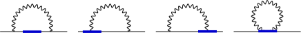
Figure 1: Feynman diagrams contributing to the one-loop calculation of the Green’s functions of operator $\mathcal{O}_{\Gamma}$. The straight (wavy) lines represent fermions (gluons). The operator insertion is denoted by a filled rectangle.

3.1 Dimensional Regularization

The perturbative calculation in $D=4-2\epsilon$ dimensions has been performed in an arbitrary covariant gauge in order to see first-hand the gauge invariance of the renormalization functions, as a consistency check. Pole parts in $\epsilon$ are multiples of the tree-level values, which indicates no mixing between operators of equal or lower dimension in the ${\overline{\rm MS}}$ scheme. Another important characteristic of the ${\cal O}(g^{2})/\epsilon$ contributions is that they are operator independent, in terms of both the Dirac structure and the length of the Wilson line, $z$. We find a gauge independent renormalization function for the operators of Eq. (2), in agreement with old results:

$$Z^{DR,\,{\overline{\rm MS}}}_{\Gamma}=1+\frac{3}{\epsilon}\,\frac{g^{2}\,C_{f}}{16\,\pi^{2}}\,,$$ (13)

While the independence of $Z^{DR,\,{\overline{\rm MS}}}_{\Gamma}$ from the Dirac matrix insertion $\Gamma$ is a feature valid to one-loop level, its independence from the length of the Wilson line $z$ is expected to hold to all orders in perturbation theory; this, in essence, is due to the fact that the most dominant pole at every loop can depend neither on the external momenta nor on the renormalization scale, thus there is no dimensionless $z$-dependent factor that could appear in the pole part.

The Green’s functions in DR are essential for the computation of the conversion factors between different renormalization schemes, and here we are interested in the RI^′ scheme defined in Eq. (11). The conversion factor is the same for each of the following pairs: ($S,\ P$), ($V_{1},\ A_{1}$), ($V_{\nu},\ A_{\nu}$), ($T_{1\nu},\ T_{\nu\rho}$). The general expressions for $\mathcal{C}_{\Gamma}$ involve integrals over modified Bessel functions; they are written out explicitly in Constantinou:2017sej . The conversion factors depend on the dimensionless quantities $z\bar{q}$ and $\bar{q}/\bar{\mu}$, where the RI’ and ${\overline{\rm MS}}$ renormalization scales ($\bar{q}$ and $\bar{\mu}$, respectively) have been left independent.

The Green’s functions of operators with a Wilson line are complex-valued; this property holds also for the non-perturbative matrix elements between nucleon states and for the conversion factors.

Note that for a scale of the form $(\bar{q},0,0,0)$ the one-loop Green’s functions are a multiple of the tree-level value of the operator under consideration. It is interesting to plot the conversion factors for the cases used in simulations, that is, $C_{V_{1}(A_{1})}$ and $C_{T}$. For convenience we choose the coupling constant and the RI’ momentum scale to match the ensemble of twisted mass fermions employed in Ref. Alexandrou:2016jqi : $g^{2}{=}3.077$, $a{=}0.082$fm, lattice size: $32^{3}\times 64$ and $a\bar{q}{=}\frac{2\pi}{32}(\frac{n_{t}}{2}{+}\frac{1}{4},0,0,n_{z})$, for $n_{t}{=}8$ and $n_{z}{=}4$ (the nucleon is boosted in the $z$ direction). The ${\overline{\rm MS}}$ scale is set to $\bar{\mu}=2{\rm GeV}$. The conversion factors are gauge dependent and we choose the Landau gauge which is mostly used in non-perturbative renormalization. In Fig. 2 we plot the real (left panel) and imaginary (right panel) parts of $C_{V_{1}(A_{1})}$ and $C_{T}$, as a function of $z/a$. One observes that for large values of $z$ the dependence of the conversion factor on the choice of operator becomes milder. However, this behavior is not granted at higher loops.

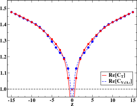
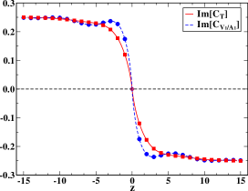
Figure 2: Real (left panel) and imaginary (right panel) parts of the conversion factors for the operators $V_{1}$ and $T$ as a function of $z/a$ in the Landau gauge. The RI’ momentum scale employed is $a\bar{q}=\frac{2\pi}{32}\left(4{+}\frac{1}{4},0,0,4\right)$.

3.2 Lattice Regularization

We now turn to the evaluation of the lattice-regularized bare Green’s functions $\langle\psi\,{\cal O}_{\Gamma_{1}}\,\bar{\psi}\rangle^{LR}$ ; this is a far more complicated calculation, as compared to dimensional regularization, because the extraction of the divergences is more delicate. Despite the complexity of the bare Green’s functions, their difference in DR and LR is necessarily independent of the external momentum $q$, which leads to a prescription for extracting $Z_{\mathcal{O}}^{LR,{\overline{\rm MS}}}$ (potentially $z$-dependent!) without an intermediate (e.g., RI^′-type) scheme.

By analogy with closed Wilson loops in regularizations other than DR, we find a linear divergence also for Wilson line operators in LR; it is proportional to $|z|/a$ and arises from the tadpole diagram, with a proportionality coefficient which depends solely on the choice of the gluon action.

Just as with other contributions to the bare Green’s function, the linear divergence is the same – at one-loop level – for all operator insertions. In a resummation of all orders in perturbation theory, the powers of $|z|/a$ are expected to exponentiate as: $\Lambda_{\Gamma}=\exp(-c\,|z|/a)\,{\tilde{\Lambda}}_{\Gamma}\,$, where $c$ is a power series in coupling, and ${\tilde{\Lambda}}_{\Gamma}$ is related to $\Lambda_{\Gamma}^{\overline{\rm MS}}$ by a further renormalization factor which is at most logarithmically divergent with $a$. To one loop, we find the following form for the difference between the bare lattice Green’s functions and the ${\overline{\rm MS}}$-renormalized ones ($\beta=1-\alpha$ is the gauge parameter):

$$\langle\psi\,{\cal O}_{\Gamma}\,\bar{\psi}\rangle^{DR,\,{\overline{\rm MS}}}-\langle\psi\,{\cal O}_{\Gamma}\,\bar{\psi}\rangle^{LR}=\frac{g^{2}\,C_{f}}{16\,\pi^{2}}\,e^{i\,q_{\mu}z}\, \Bigg{[} \Gamma\Big{(}\alpha_{1}+\alpha_{2}\,\beta+\alpha_{3}\,\frac{|z|}{a}+\log\left(a^{2}\bar{\mu}^{2}\right)\left(4-\beta\right)\Big{)}$$ (14)

$$+\left(\Gamma\cdot\gamma_{\mu}+\gamma_{\mu}\cdot\Gamma\right)\,\Big{(}\alpha_{4}+\alpha_{5}\,c_{\rm SW}\Big{)}\Bigg{]}\,.$$

Using Eq. (14) together with Eq. (9) one can extract the gauge invariant multiplicative renormalization and mixing coefficients in the ${\overline{\rm MS}}$-scheme and LR. In our calculation $\alpha_{3}$ is negative, as expected.

A few interesting properties of Eq. (14) can be pointed out: The contribution $\left(\Gamma\cdot\gamma_{\mu}{+}\gamma_{\mu}\cdot\Gamma\right)$ indicates mixing between operators of equal dimension, which is finite and appears in the lattice regularization. Moreover, this combination vanishes for certain choices of the Dirac structure $\Gamma$ in the operator. For the operators $P$, $V_{\nu}$ ($\nu\neq\mu$), $A_{\mu}$, $T_{\mu\nu}$ ($\nu\neq\mu$) the combination $\left(\Gamma\cdot\gamma_{\mu}+\gamma_{\mu}\cdot\Gamma\right)$ is zero and only a multiplicative renormalization is required. This has significant impact in the non-perturbative calculation of the unpolarized quasi-PDFs, as there is a mixing with a twist-3 scalar operator. Such a mixing must be eliminated using a proper renormalization prescription, ideally non-perturbatively Alexandrou:2017huk .

To one-loop level, the diagonal elements of the mixing matrix (multiplicative renormalization) are the same for all operators under study, and through Eq. (9) one obtains:

$$Z_{\Gamma}^{LR,{\overline{\rm MS}}}=1+\frac{g^{2}\,C_{f}}{16\,\pi^{2}}\,\left(e_{1}+e_{2}\,\frac{|z|}{a}+e_{3}\,c_{\rm SW}+e_{4}\,c_{\rm SW}^{2}-3\log\left(a^{2}\bar{\mu}^{2}\right)\right),$$ (15)

where the coefficients $e_{1}-e_{4}$ are given in Table 1, for different gluon actions. As expected, $Z_{\Gamma}^{LR,{\overline{\rm MS}}}$ is gauge independent, and the cancelation of the gauge dependence was numerically confirmed up to ${\cal O}(10^{-5})$. This gives an estimate on the accuracy of the numerical loop integrations. Similar to $Z_{\Gamma}^{LR,{\overline{\rm MS}}}$, the nonvanishing mixing coefficients are operator independent and have the general form:

$$Z_{12}^{LR,{\overline{\rm MS}}}=Z_{21}^{LR,{\overline{\rm MS}}}=0+\frac{g^{2}\,C_{f}}{16\,\pi^{2}}\,\left(e_{5}+e_{6}\,c_{\rm SW}\right),$$ (16)

where $Z_{ij}^{LR,{\overline{\rm MS}}}$ ($i\neq j$) is nonzero only for the operator pairs: $\{S,\,V_{1}\}$, $\{A_{2},\,T_{34}\}$, $\{A_{3},\,T_{42}\}$, $\{A_{4},\,T_{23}\}$. The coefficients $e_{5}$ and $e_{6}$ are shown in Table 1. Given that the strength of mixing depends on the value of $c_{\rm SW}$, one may tune the clover parameter in order to eliminate mixing at one loop.

Table 1: Numerical values of the coefficients $e_{1}$ - $e_{4}$ of the multiplicative renormalization functions and $e_{5}$ - $e_{6}$ of the mixing coefficients for Wilson, tree-level (TL) Symanzik and Iwasaki gluon actions.

Action	$e_{1}$	$e_{2}$	$e_{3}$	$e_{4}$	$e_{5}$	$e_{6}$
Wilson	24.3063	-19.9548	-2.24887	-1.39727	14.4499	-8.28467
TL Symanzik	19.8442	-17.2937	-2.01543	-1.24220	12.7558	-7.67356
Iwasaki	12.5576	-12.9781	-1.60101	-0.97321	9.93653	-6.52764

The linear divergence in the lattice-regularized Wilson line operator requires a careful removal before the continuum limit can be reached in the non-perturbative matrix elements. One way to eliminate this divergence is to use the estimate of the one-loop coefficient $e_{2}$ of Eq. (15) and subtract it from the non-perturbative matrix elements. However, this subtraction only partially removes the divergence, as higher orders still remain and they will dominate in the $a\to 0$ limit. Thus, it is preferable to develop a non-perturbative method to extract the linear divergence.

Our proposal is based on using bare matrix elements of the Wilson line operators from numerical simulations, denoted by $q(P_{3},z)$ in Ref. Alexandrou:2016jqi . We focus on the helicity (axial) and transversity (tensor); these exhibit no mixing. In non-perturbative calculations, the nucleon is boosted by momentum $P_{3}$ along the direction of the Wilson line. Based on the arguments presented in the previous Subsection we expect that the renormalized matrix elements can depend on $z$ only through the dimensionless quantity $P_{3}z$. Furthermore, the dependence on the scale $\bar{\mu}$ in the renormalized matrix element is well defined and involves the anomalous dimension ($\gamma_{\Gamma}$) of the operator: $q^{R}(P_{3}z,P_{3}/\bar{\mu})\propto{\bar{\mu}}^{-2\gamma_{\Gamma}}$, which is matched by the $\bar{\mu}$ dependence in the renormalization function. Thus,

$$q^{R}(P_{3}z,P_{3}/\bar{\mu})=(P_{3}/\bar{\mu})^{2\gamma_{\Gamma}}\cdot{\tilde{q}}^{R}(P_{3}z).$$ (17)

Similarly, the function $Z_{\Gamma}^{LR,{\overline{\rm MS}}}(a\bar{\mu},z/a)$, given its expected $\bar{\mu}$-dependence, will factorize as:

$$Z_{\Gamma}^{LR,{\overline{\rm MS}}}(a\bar{\mu},z/a)={\tilde{Z}}_{\Gamma}(a\bar{\mu})\cdot\hat{Z}(z/a).$$ (18)

The factor $\hat{Z}(z/a)$ originates exclusively from tadpole diagrams; the one-loop contribution proportional to $e_{2}$ in Eq. (15) will exponentiate, upon considering higher powers of $g$, leading to:

$$\hat{Z}(z/a)=e^{-\delta m\,|z|/a},\qquad\delta m=-\frac{g^{2}\,C_{f}}{16\,\pi^{2}}\,e_{2}+{\cal O}(g^{4}).$$ (19)

This is entirely consistent with the exponential behavior $\exp(-\delta m\,|z|/a)$ proven for Wilson loops.

We can thus write the ratio of the bare matrix elements for different values of $P_{3}$ and $z$ as:

$$\frac{q(P_{3},z)}{q(P^{\prime}_{3},z^{\prime})}=\frac{Z_{\Gamma}^{LR,{\overline{\rm MS}}}(a\bar{\mu},z/a)\cdot q^{R}(P_{3}z,P_{3}/\bar{\mu})}{Z_{\Gamma}^{LR,{\overline{\rm MS}}}(a\bar{\mu},z^{\prime}/a)\cdot q^{R}(P^{\prime}_{3}z^{\prime},P^{\prime}_{3}/\bar{\mu})}=\frac{e^{-\delta m\,|z|/a}\,\tilde{Z}_{\Gamma}(a\bar{\mu})\,\left({\displaystyle\frac{P_{3}}{\bar{\mu}}}\right)^{2\gamma_{\Gamma}}\,\tilde{q}^{R}(P_{3}z)}{e^{-\delta m\,|z^{\prime}|/a}\,\tilde{Z}_{\Gamma}(a\bar{\mu})\,\left({\displaystyle\frac{P^{\prime}_{3}}{\bar{\mu}}}\right)^{2\gamma_{\Gamma}}\,\tilde{q}^{R}(P^{\prime}_{3}z^{\prime})}\,,$$ (20)

where the one-loop anomalous dimension is $\gamma_{\Gamma}=-3g^{2}C_{f}/(16\pi^{2})$ for all operator insertions. Choosing $P_{3},\,P^{\prime}_{3},\,z,\,z^{\prime}$ such that $P_{3}z=P^{\prime}_{3}z^{\prime}$, simplifies the ratio considerably:

$$q(P_{3},z)/q(P^{\prime}_{3},z^{\prime})=e^{-\delta m\,(|z|-|z^{\prime}|)/a}\,(P_{3}/P^{\prime}_{3})^{-6g^{2}C_{f}/(16\pi^{2})}\,.$$ (21)

Thus, by forming this ratio from non-perturbative data, and by choosing several combinations of $P_{3}z=P^{\prime}_{3}z^{\prime}$, one can fit to extract the coefficient of the linear divergence, $\delta m$. This ratio can be investigated for the helicity and transversity separately. Since the right-hand side of Eq. (21) is independent of the operator insertion, one expects the same value for the exponential coefficient, up to lattice artifacts. We have tested this method with the data of ETMC presented in Ref. Alexandrou:2016jqi , with encouraging results: $\bullet$ The ratio $q(P_{3},z)/q(P^{\prime}_{3},z^{\prime})$ was found to be real for the helicity and transversity as expected from Eq. (21), despite the fact that the matrix elements themselves are complex $\bullet$ The analogous ratio for the unpolarized operator, which mixes with the scalar, leads to a nonzero imaginary part $\bullet$ The extracted value for the coefficient $\delta m/a$, using different combinations of $P_{3}z$, is consistent within statistical accuracy $\bullet$ Both helicity and transversity give very similar estimates for $\delta m/a$.

4 Future Work

A natural continuation of this project is the addition of smearing to the fermionic part of the action and/or to the gauge links of the Wilson line operator. This is important, as modern simulations employ such smearing techniques (e.g., stout and HYP) that suppress the power divergence and bring the renormalization functions closer to their tree-level values. Smearing the operator under study alters its renormalization functions, thus, the same smearing must be employed in the renormalization process.

An extension of this calculation that we intend to pursue, is the evaluation of lattice artifacts to one loop and to all orders in the lattice spacing, ${\cal O}(a^{\infty},\,g^{2})$. This has been successfully applied to local and one-derivative fermion operators suppressing lattice artifacts from non-perturbative estimates. For operators with a long Wilson line ($z{>>}a$) the lattice artifacts are likely to be more prominent, and therefore, such a calculation will be extremely beneficial for non-perturbative renormalization.

A possible addition to the present work is the two-loop calculation in DR, from which one can extract the conversion factor between different renormalization schemes, as well as the anomalous dimension of the operators. The conversion factor up to two loops may be applied to non-perturbative data on the renormalization functions, to bring them to the ${\overline{\rm MS}}$-scheme at a better accuracy. Nonzero renormalized masses in the conversion factors, and differences between flavor-singlet and -nonsinglet operators would further improve accuracy.

Finally, the techniques developed in this work for the renormalization of quasi-PDFs may be inspiring for the renormalization of Wilson-line fermion operators of different structure, such as staples. This will be of high importance for matrix elements of the transverse momentum-dependent parton distributions (TMDs) that are currently under investigation for the nucleon and pion in lattice QCD.

Acknowledgments: We would like to thank the members of ETMC, in particular Krzysztof Cichy, for fruitful discussions. MC acknowledges financial support by the U.S. Department of Energy, Office of Science, Office of Nuclear Physics, within the framework of the TMD Topical Collaboration, as well as by the National Science Foundation under Grant No. PHY- 1714407.

References

- (1) M. Constantinou, H. Panagopoulos, Phys. Rev. D96, 054506 (2017), 1705.11193
- (2) C. Alexandrou, K. Cichy, M. Constantinou, K. Hadjiyiannakou, K. Jansen, H. Panagopoulos, F. Steffens, Nucl. Phys. B923, 394 (2017), 1706.00265
- (3) C. Alexandrou, K. Cichy, M. Constantinou, K. Hadjiyiannakou, K. Jansen, F. Steffens, C. Wiese, Phys. Rev. D96, 014513 (2017), 1610.03689