Classical and relativistic models for time duration of gamma-ray bursts

Abstract

A classical model based on a power law assumption for the radius-time relationship in the expansion of a Supernova (SN) allows to derive an analytical expression for the flow of mechanical kinetic energy and the time duration of Gamma-ray burst (GRB). A random process based on the ratio of two truncated lognormal distributions for luminosity and luminosity distance allows to derive the statistical distribution for time duration of GRBs. The high velocities involved in the first phase of expansion of a SN requires a relativistic treatment. The circumstellar medium is assumed to follow a density profile of Plummer type with eta=6. A series solution for the relativistic flow of kinetic energy allows to derive in a numerical way the duration time for GRBs. Here we analyse two cosmologies: the standard cosmology and the plasma cosmology.

Keywords: Cosmology; Observational cosmology; Distances, redshifts, radial velocities, spatial distribution of galaxies;

1 Introduction

The theoretical efforts for gamma-ray bursts (GRBs) analyze: (i) the different predictions between cannonball and fireball model, see [1, 2], (ii) the acceleration of ultrahigh-energy cosmic rays (UHECRs) at the afterglow phase, see [3], (iii) a possible connection with High-energy neutrinos (HEN) and gravitational waves (GW), see [4], (iv) the frames of Hypersphere World-Universe Model (WUM), see [5]. We briefly recall that the time duration for Gamma-ray burst (GRB) is measured without the knowledge of the redshift, see as an example [6]. The distance of GRBs is therefore unknown and the galactic or extra-galactic origin should be analyzed. We test therefore in the following the reliability of time duration for GRBs along two astrophysical hypothesis: (i) the GRBs are generated in external galaxies, (ii) the GRBs are connected with the light curve (LC) of a Supernova (SN). A first classification of time duration provides a division between short and long GRBs, with the boundary at $\approx$ 2 s, see [7]. The form of the probability density function (PDF) which produces the better fit to the sequence of times is also subject of research, as an example a two Gaussian-fits has been suggested by [8] and a lognormal PDF by [9].

This paper reviews in Section 2 the current status of the observations for the time duration of GRBs. Section 3 develops a simple classic model for theoretical time duration for GRBs. Section 4 contains a simulation for time duration of GRBs based on the random generation of luminosity and distance luminosity. Section 5 derives a relativistic equation of motion for SN, deduces the relativistic flow of energy and finally evaluates the time duration for GRBS in a relativistic environment.

2 Preliminaries

This section reviews the observations of the Fermi Gamma-ray Burst Monitor (GBM) for the time duration and fits the data with the truncated lognormal PDF.

2.1 The observations

Most of the typical GRBs have two stages: the initial prompt emission phase observed in the gamma-ray band and the following afterglow phase with multi-bands’ emission. The observational time duration is measured during the prompt emission phase with the typical energy band between tens of keV to hundreds of keV. Observationally, the light curve of the afterglow phase can be fitted by a broken power-law, but the light curve during the prompt emission phase is highly variable and completely different from the afterglow phase. The time duration of GRBs has been monitored by GBM in the $50-300$ keV energy range, see the third catalog [6] which is available on line at http://cdsweb.u-strasbg.fr/. The above catalog reports two times of burst duration $T_{50}$ and $T_{90}$ which are defined as the interval between the times where the burst has reached $25\%$ and $75\%$ of its maximum fluence. Figure 1 reports the sky distribution of GRBs in Galactic coordinates.

Figure 1: Sky distribution of GRBs in Galactic coordinates projected using the Mollweide projection.

A simple test on the isotropy of the arrival direction of GRBs can be performed dividing the the surface area of a sphere of unit radius in $N\times N$ boxes of equal area. We then choose $N$ in order to have $\approx\,7$ theoretical events, $n_{th}$, assuming a uniform distribution on the total surface area, which means $N=14$. We now evaluate the observed averaged number of GRBs in each box, $n$, which turns out to be $n=7.16\pm 2.7$. The goodness of the isotropy is evaluated through the percentage error, $\delta$, which is

$$\delta=\frac{\big{|}n_{th}-n\big{|}}{n_{th}}\times 100\quad=2.4\%\quad.$$ (1)

The low value of the percentage error for the isotropy allows to state that:

• the GRBs have an extra-galactic origin

• the spatial distribution of GRBs is isotropic.

The histogram of time distribution for GRBs for the case of $T_{50}$ in Figure 2 and in Figure 3 for the case of $T_{90}$

Figure 2: Frequencies distribution (linear scale)) of $T_{50}$ (decimal logarithm scale) for GRBs.

Figure 3: Frequencies distribution (linear scale)) of $T_{90}$ (decimal logarithm scale) for GRBs.

Tables 1 and 2 report the main statistical parameters of $T_{50}$ and $T_{90}$ respectively.

Table 1: The sample parameters of $T_{50}$ for GRBs in seconds.

$$\begin{array}[]{ll}\hline\cr Parameter&value~{}(seconds)\\ \vskip 3.0pt plus 1.0pt minus 1.0pt\cr\hline\cr\vskip 3.0pt plus 1.0pt minus 1.0pt\cr elements&1405\\ maximum&736.51\\ mean&18.23\\ minimum&0.016\\ standard~{}deviation&41.22\\ \hline\cr\end{array}$$

Table 2: The sample parameters of $T_{90}$ for GRBs in seconds.

$$\begin{array}[]{ll}\hline\cr Parameter&value~{}(seconds)\\ \vskip 3.0pt plus 1.0pt minus 1.0pt\cr\hline\cr\vskip 3.0pt plus 1.0pt minus 1.0pt\cr elements&1405\\ maximum&828.67\\ mean&39.64\\ minimum&0.048\\ standard~{}deviation&62.55\\ \hline\cr\end{array}$$

2.2 The fit

The high number of decades, $\approx$ 4, covered by the distribution of $T_{50}$ and $T_{90}$ suggests to fit the data with the truncated lognormal (TL) PDF

$$TL(x;m,\sigma,x_{l},x_{u})=$$

$$\frac{\sqrt{2}{{\rm e}^{-\frac{1}{2}\,{\frac{1}{{\sigma}^{2}}\left(\ln\left({\frac{x}{m}}\right)\right)^{2}}}}}{\sqrt{\pi}\sigma\,\left(-{\rm erf}\left(\frac{1}{2}\,{\frac{\sqrt{2}}{\sigma}\ln\left({\frac{x_{{l}}}{m}}\right)}\right)+{\rm erf}\left(\frac{1}{2}\,{\frac{\sqrt{2}}{\sigma}\ln\left({\frac{x_{{u}}}{m}}\right)}\right)\right)x}\quad,$$ (2)

where $x$ is the random variable, $x_{l}$ is the lower bound, $x_{u}$ is the upper bound, $m$ is the scale parameter and $\sigma$ is the shape parameter, see [10] for more details. Tables 3 and 4 report the four parameters of the TL for $T_{50}$ and $T_{90}$ respectively. Table 4 reports also the parameters of the lognormal PDF as well the maximum distance, $d_{max}$, between the theoretical and the observed distribution function (DF) in the Kolmogorov–Smirnov test (K–S), see [11, 12, 13].

The DF is

$$DF(x;m,\sigma,x_{l},x_{u})=\frac{-{\rm erf}\left(\frac{1}{2}\,{\frac{\sqrt{2}}{\sigma}\ln\left({\frac{x}{m}}\right)}\right)+{\rm erf}\left(\frac{1}{2}\,{\frac{\sqrt{2}}{\sigma}\ln\left({\frac{x_{{l}}}{m}}\right)}\right)}{{\rm erf}\left(\frac{1}{2}\,{\frac{\sqrt{2}}{\sigma}\ln\left({\frac{x_{{l}}}{m}}\right)}\right)-{\rm erf}\left(\frac{1}{2}\,{\frac{\sqrt{2}}{\sigma}\ln\left({\frac{x_{{u}}}{m}}\right)}\right)}\quad.$$ (3)

A random generation of the variate X can be found by solving the following non linear equation

$$R=DF(X;m,\sigma,x_{l},x_{u})\quad,$$ (4)

where $R$ is the unit rectangular variate.

Table 3: The TL parameters of $T_{50}$ for GRBs.

$$\begin{array}[]{ll}\hline\cr Parameter&value\\ \vskip 3.0pt plus 1.0pt minus 1.0pt\cr\hline\cr\vskip 3.0pt plus 1.0pt minus 1.0pt\cr elements&1405\\ x_{l}&0.016\\ x_{u}&736.51\\ m&5.33\\ \sigma&1.89\\ \hline\cr\end{array}$$

Table 4: The TL PDF and lognormal PDF parameters of $T_{90}$ for GRB.

$$\begin{array}[]{lll}\hline\cr Parameter&value~{}TL&value~{}lognormal\\ \vskip 3.0pt plus 1.0pt minus 1.0pt\cr\hline\cr\vskip 3.0pt plus 1.0pt minus 1.0pt\cr elements&1405&1405\\ x_{l}&0.048&0\\ x_{u}&828.6&\infty\\ m&14.62&13.57\\ \sigma&1.911&1.8\\ d_{max}&0.096&0.1\\ \hline\cr\end{array}$$

3 A classical model for the light curve

We assume that the observed radius–time relationship, $R(t)$, for SN has a power law dependence of the type

$$R(t)=C\times t^{\alpha}\quad,$$ (5)

where $C$ is a constant and $\alpha$ a parameter which can be fixed by the observation of the temporal evolution of the radius of a SN, in the case of SN 1993J   $\alpha=0.82$, see [14]. At time $t_{0}$ the radius $R_{0}$ is

$$R_{0}(t)=C\times t_{0}^{\alpha}\quad.$$ (6)

The velocity, $V(t)$, is

$$V(t)=C\times\alpha t^{(\alpha-1)}\quad,$$ (7)

and the velocity at time $t_{0}$ is

$$V_{0}(t)=C\times\alpha t_{0}^{(\alpha-1)}\quad.$$ (8)

In classical physics the density of kinetic energy, $K$, is

$$K=\frac{1}{2}\rho V^{2}\quad,$$ (9)

where $\rho$ is the density and $V$ the velocity. In presence of an area $A$ and when the velocity is perpendicular to that area, the mechanical flux of kinetic energy $L_{m}$ is

$$L_{m}=\frac{1}{2}\rho AV^{3}\quad,$$ (10)

which in SI is measured in $W$ and in CGS in erg $s^{-1}$ see formula (A28) in [15]. In our case, $A=4\pi R^{2}$, which means

$$L_{m}=\frac{1}{2}\rho 4\pi R^{2}V^{3}\quad.$$ (11)

The density in the advancing layer as function of the radius, $\rho(R)$, is assumed to scale as

$$\rho(R)=\rho_{0}(\frac{R}{R_{0}})^{-d}\quad,$$ (12)

where $\rho_{0}$ is the density at radius $R_{0}$. According to previous formula the scaling law for the mechanical luminosity as function of the time is

$$L_{m}=L_{m,0}\bigl{(}\frac{t}{t0}\bigr{)}^{5\,\alpha-d\alpha-3}\quad,$$ (13)

where $L_{m,0}$ is the mechanical luminosity at $t=t_{0}$. The observed luminosity at a given frequency $\nu$, $L$, is assumed to be proportional to the mechanical luminosity

$$L=\epsilon L_{m}\quad,$$ (14)

where $\epsilon$ is a constant of conversion. The luminosity at a given range of energy is expressed in $\frac{erg}{s}$ in CGS and $W$ in SI. As a useful example the astrophysical version of the luminosity at $t=t_{0}$ is

$$L=2.68521\,{\it n_{0}}\,({{\it R_{0,pc}}})^{2}({\frac{V_{0}}{c}})^{3}\,10^{32}\,W\quad,$$ (15)

where $R_{0,pc}$ is the radius at $t=t_{0}$ in pc, $V_{0}$ is the velocity at $t=t_{0}$ in $\frac{km}{s}$, $c$ is the light velocity in $\frac{km}{s}$ and $n_{0}$ is the number density expressed in particles $\mathrm{cm}^{-3}$ (density $\rho_{0}=n_{0}m$, where $m=m_{\mathrm{H}}$).

The observed flux, $F$, as a function of the luminosity distance, $D_{L}$, is

$$F=\frac{L}{4\pi D^{2}}\quad,$$ (16)

or

$$F(L,D_{L})=\frac{L_{0}\bigl{(}\frac{t}{t0}\bigr{)}^{5\,\alpha-d\alpha-3}}{4\pi D_{L}^{2}}\quad,$$ (17)

where $L_{0}=\epsilon L_{m,0}$. The observed flux at a given range of energy is expressed in $\frac{erg}{s\,cm^{2}}$ in CGS and $\frac{W}{m^{2}}$ in SI. An on line collection of light curves for GRBs is made by the Swift GRB Mission and can be found at http://swift.gsfc.nasa.gov/index.html, see also [16, 17]: the band of the observations is (0.3-10) kev. As a practical example we processed GRB 161214B , see [18], with review data in Table 5, and real data available at http://www.swift.ac.uk/xrt_curves/00726885/. Figure 4 displays the LC of such burst as well a power law fit.

Table 5: Some parameters of GRB 161214B .

$$\begin{array}[]{ll}\hline\cr Parameter&value\\ \vskip 3.0pt plus 1.0pt minus 1.0pt\cr\hline\cr\vskip 3.0pt plus 1.0pt minus 1.0pt\cr date&16/12/14\\ T_{50}(s)&9.67\\ T_{90}(s)&24.82\\ C_{k}~{}t<100\,s&8.43\times 10^{-5}\\ k~{}~{}~{}t<100\,s&-2.54\\ \hline\cr\end{array}$$

Figure 4: Light curve of GRB 161214B in the first 100 seconds (empty stars) and power law fit (dotted line).

A first numerical analysis of the observed flux, $F_{0}$, versus time relationship can be done by assuming a power law dependence

$$F_{0}(t)=C_{k}t^{k}\,erg\,s^{-1}\quad,$$ (18)

where the two parameters $C$ and $k$ are found from a numerical analysis of the data, see Table 5. We now match the observed value of $k$ with the theoretical exponent given by equation (17)

$$k=5\,\alpha-d\alpha-3\quad.$$ (19)

The above equation allows to deduce $d$ once $\alpha$ and $k$ are given: as an example, when $\alpha=0.82$ and $k=-2.54$, $d=4.44$. The decreasing flux will be visible until a minimum value of threshold in the flux $F_{T}$ is reached. As an example the instrument Windowed Timing (WT) of X-ray telescope (XRT) on the Swift satellite has a threshold value of $F_{T}\approx 3.1\frac{fW}{m^{2}}$. Therefore the GRB will be visible up to a maximum value in time of $t_{max}$

$$t_{max}=t_{0}(\frac{F_{T}4\pi D_{L}^{2}}{L_{0}})^{\frac{1}{5\,\alpha-d\alpha-3}}\quad,$$ (20)

or

$$t_{max}=t_{0}(\frac{F_{T}}{F_{0}})^{\frac{1}{5\,\alpha-d\alpha-3}}\quad,$$ (21)

where $F_{0}$ is the observed flux at $t=t_{0}$.

4 The simulation

A simulation of the duration time for GRBs according to equation 20 requires the ratio of two two lognormal PDFs ( one for $L_{0}$ and the other one for $D_{L}$) and a cosmological environment.

4.1 The ratio of two lognormal PDFs

We now evaluate the mean and the variance of the ratio of two lognormal distributions , $\frac{X}{Y}$. From the fact that $\ln(\frac{X}{Y})=\ln(X)-\ln(Y)$ and $X$ and $Y$ are lognormally distributed, it turns out that $\ln(X)$ and $\ln(Y)$ are distributed as a normal PDF. We assume that $\ln(X)$ and $\ln(Y)$ have means $\mu_{X}$ and $\mu_{Y}$, variances $\sigma^{2}_{X}$ and $\sigma^{2}_{Y}$ , and covariance $\sigma^{2}_{XY}$ (equal to zero if X and Y are independent) and are jointly normally distributed. The difference $Z$ is then distributed as a normal PDF with mean $\mu_{Z}=\mu_{X}-\mu_{Y}$ and variance $\sigma^{2}_{Z}$ = $\sigma^{2}_{X}$ + $\sigma^{2}_{Y}$ - 2 $\sigma^{2}_{XY}$.

Note that $\frac{X}{Y}=\exp(Z)$ , which means that $\frac{X}{Y}$ is distributed as a lognormal PDF with parameters $\mu_{Z}$ and $\sigma^{2}_{Z}$.

4.2 Cosmological models

We deal with two cosmologies: the $\Lambda$CDM cosmology and the plasma cosmology. The the $\Lambda$CDM cosmology is characterized by three parameters which are the Hubble constant, $H_{0}$, expressed in $\mathrm{km\,s^{-1}\,Mpc^{-1}}$ and the two numbers $\Omega_{\rm M}$ and $\Omega_{\Lambda}$, see Table 6.

Table 6: Numerical values for parameters of the two cosmologies.

$$\begin{array}[]{ccccc}\hline\cr cosmology&compilation&H_{0}~{}in~{}\mathrm{km\,s^{-1}\,Mpc^{-1}}&\Omega_{\rm M}&\Omega_{\Lambda}\\ \hline\cr\Lambda\!CDM&~{}Union~{}2.1&69.81&0.239&0.651\\ plasma&~{}Union~{}2.1&74.2&{}\hfil&{}\hfil\\ \hline\cr\end{array}$$

A simple expression for the luminosity distance, $D_{l}$, in $\Lambda$CDM is obtained with the minimax approximation ($p=3,q=2$)

$$D_{\rm L,3,2}=$$

$$\frac{0.3597252600+5.612031882\,z+5.627811123\,{z}^{2}+0.05479466285\,{z}^{3}}{0.0105878216+0.1375418627\,z+0.1159043801\,{z}^{2}}.$$ (22)

More details on the analytical derivation of the luminosity distance in terms of Padé approximant can be found in [19].

The plasma cosmology is characterized by one parameter which is $H_{0}$ and by a simple formula for the luminosity distance which is the same of the distance, $d_{p}$,

$$D_{L}(z;H_{0})\equiv d_{p}(z;H_{0})=$$

$$\frac{0.359725+5.61203\,z+5.62781\,{z}^{2}+0.0547946\,{z}^{3}}{0.010587+0.137541\,z+0.115904\,{z}^{2}}\quad,$$ (23)

see [20, 21, 22, 23] and Table 6.

A careful examination of equation (20) which gives the time duration for a GRB isolates five fixed basic parameters which are $\alpha$, $d$, $R_{0}$, $V_{0}$,$t_{0}$ and two random parameters are , $L$,$D_{L}$. In order to allow the simulation the five fixed parameters are reported in Table 7.

Table 7: The fixed parameters of the simple model.

$$\begin{array}[]{cc}\hline\cr Parameter&value\\ \hline\cr t_{0}~{}(s)&0.1\\ R_{0}~{}(pc)&0.06\\ V_{0}~{}(\frac{km}{s})&200000\\ \alpha&0.8288\\ d&3.075\\ \hline\cr\end{array}$$

The variable $L$ is generated in a random way which follows a TL PDF with the following meanings: $L_{l}$ lower luminosity, $L_{u}$ upper luminosity and $L^{*}$ the scale, see Table 8.

Table 8: The parameters of the simulation for $L$ in $\Lambda$CDM and plasma cosmology.

$$\begin{array}[]{cccc}\hline\cr Parameter&\Lambda\!CDM~{}cosmology&Plasma~{}cosmology\\ \hline\cr x_{l}=\frac{L_{l}}{10^{51}erg\,s^{-1}}&8.11\,10^{-6}&1.77\,10^{-9}\\ x_{u}=\frac{L_{u}}{10^{51}erg\,s^{-1}}&4.05\,10^{-2}&2.36\,10^{-3}\\ m=\frac{L^{*}}{10^{51}erg\,s^{-1}}&4.05\,10^{-5}&5.9\,10^{-9}\\ \sigma&2.0&1.8\\ \hline\cr\end{array}$$

The theoretical luminosity at $t=t_{0}$, $L_{0}$, is obtained inserting in equation (15) the number density $n_{0}$ for which $L=L_{0}$.

The variable $D_{L}$, in the case of $\Lambda$CDM or plasma cosmology, is generated in a random way which follows a TL PDF with the following meanings: $D_{L,l}$ lower luminosity distance, $L_{L,u}$ upper luminosity distance and $m$ the scale , see Table 9.

Table 9: The parameters of the simulation for $D_{L}$ in $\Lambda$CDM and plasma cosmology.

$$\begin{array}[]{cccc}\hline\cr Parameter&\Lambda\!CDM~{}cosmology&Plasma~{}cosmology\\ \hline\cr D_{L,l}\,(Mpc)&3&1\\ D_{L,u}\,(Mpc)&40000&5000\\ m\,(Mpc)&700&181.45\\ \sigma&1.8&1.19\\ \hline\cr\end{array}$$

Once a sequence of theoretical times of duration is obtained according to equation (20), see results in Table 10, we compare the observed and simulated data, see Figures 5 and 6.

Table 10: Theoretical time duration for GRBs in seconds.

$$\begin{array}[]{lll}\hline\cr Parameter&\Lambda\!CDM~{}cosmology&Plasma~{}cosmology\\ \vskip 3.0pt plus 1.0pt minus 1.0pt\cr\hline\cr\vskip 3.0pt plus 1.0pt minus 1.0pt\cr elements&1405&1405\\ maximum~{}(s)&3875.1&433\\ mean~{}(s)&36.2&16.84\\ minimum~{}(s)&0.828&0.162\\ standard~{}deviation(s)&140.2&48.22\\ \hline\cr\end{array}$$

The theoretical reason which allows to fit the ratio of two lognormal PDFs with another lognormal is outlined in Section 4.1.

Figure 5: Frequencies distribution (linear scale)) of $T_{90}$ (decimal logarithm scale) for GRBs (full line) and theoretical simulation in the case of the $\Lambda$CDM cosmology (dotted line) with parameters as in Tables 8 and 9.

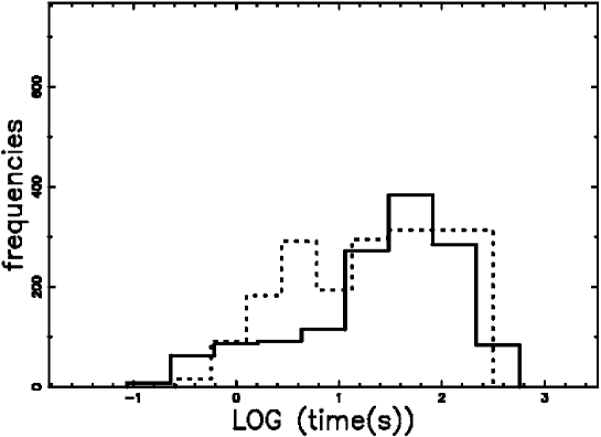
Figure 6: Frequencies distribution (linear scale) of $T_{90}$ (decimal logarithm scale) for GRBs (full line) and theoretical simulation in the case of the plasma cosmology (dotted line) with parameters as in Tables 8 and 9.

5 Relativistic case

The density, $\rho$, of the ISM at a distance $r$ from the SN is here modeled by a Plummer-like profile, see [24],

$$\rho(r;R_{flat})=\rho_{c}({\frac{R_{flat}}{({R_{flat}^{2}+r^{2}})^{1/2}}})^{\eta}\quad.$$

where $r$ is the distance from the center, $\rho$ is the density, $\rho_{c}$ is the density at the center, $R_{flat}$ is the distance before which the density is nearly constant, and $\eta$ is the power law exponent at large values of $r$. The following transformation, $R_{flat}=\sqrt{3}b$, gives

$$\rho(r;b)=\rho_{c}\bigl{(}\frac{1}{1+\frac{1}{3}\,{\frac{{r}^{2}}{{b}^{2}}}}\bigr{)}^{\eta/2}\quad.\quad$$ (24)

The total mass $M(r;b)$ comprised between 0 and $r$, when $\eta=6$, is

$$M(r;b)=\int_{0}^{r}4\pi r^{2}\rho(r;b)dr=\frac{3}{2}\,{\frac{\rho\_c,\pi\,{b}^{3}}{(3\,{b}^{2}+{r}^{2})^{2}}\Bigl{(}9\,\arctan(\frac{1}{3}\,{\frac{r\sqrt{3}}{b}})\sqrt{3}{b}^{4}}$$

$${+6\,\arctan(\frac{1}{3}\,{\frac{r\sqrt{3}}{b}})\sqrt{3}{b}^{2}{r}^{2}}{+\arctan(\frac{1}{3}\,{\frac{r\sqrt{3}}{b}})\sqrt{3}{r}^{4}-9\,{b}^{3}r+3\,b{r}^{3}\Bigr{)}}\quad.$$ (25)

The relativistic conservation of momentum, see [25, 26, 27], states that

$$M(R_{0};b)\gamma_{0}\beta_{0}=M(r;b)\gamma\beta\quad,$$

with

$$\gamma_{0}=\frac{1}{\sqrt{1-\beta_{0}^{2}}}\quad;\qquad\gamma=\frac{1}{\sqrt{1-\beta^{2}}}\quad,$$

and

$$\beta_{0}=\frac{V_{0}}{c}\quad;\qquad\beta=\frac{v}{c}\quad,$$

where $R_{0}$ is the initial radius of the advancing sphere, $V_{0}$ is the initial velocity at $R_{0}$ and $c$ is the light velocity.

The relativistic conservation of momentum for a Plummer profile with $\eta=6$ is

$$\frac{AN}{AD}=\frac{BN}{BD}\quad,$$ (26)

$$AN=3\,\,\pi\,{b}^{3}\Bigl{(}9\,\arctan(\frac{1}{3}\,{\frac{r(t)\sqrt{3}}{b}})\sqrt{3}{b}^{4}+6\,\arctan(\frac{1}{3}\,{\frac{r(t)\sqrt{3}}{b}})\sqrt{3}{b}^{2}(r(t))^{2}$$

$$+\arctan(\frac{1}{3}\,{\frac{r(t)\sqrt{3}}{b}})\sqrt{3}(r(t))^{4}-9\,{b}^{3}r(t)+3\,b(r(t))^{3}\Bigr{)}{\frac{\rm d}{{\rm d}t}}r(t)$$ (27)

$$AD=2\,\left(3\,{b}^{2}+\left(r\left(t\right)\right)^{2}\right)^{2}c\sqrt{1-{\frac{\left({\frac{\rm d}{{\rm d}t}}r\left(t\right)\right)^{2}}{{c}^{2}}}}\quad,$$ (28)

$$BN=3\,\,\pi\,{b}^{3}\Bigl{(}9\,\arctan(\frac{1}{3}\,{\frac{R_{{0}}\sqrt{3}}{b}})\sqrt{3}{b}^{4}+6\,\arctan(\frac{1}{3}\,{\frac{R_{{0}}\sqrt{3}}{b}})\sqrt{3}{b}^{2}{R_{{0}}}^{2}$$

$$+\arctan(\frac{1}{3}\,{\frac{R_{{0}}\sqrt{3}}{b}})\sqrt{3}{R_{{0}}}^{4}-9\,{b}^{3}R_{{0}}+3\,b{R_{{0}}}^{3}\Bigr{)}\beta_{{0}}\quad,$$ (29)

$$BD=2\,\left(3\,{b}^{2}+{R_{{0}}}^{2}\right)^{2}\sqrt{1-{\beta_{{0}}}^{2}}\quad.$$ (30)

The relativistic transfer of energy through a surface, $A$, is

$$L_{m,r}=A\gamma^{2}(\rho c^{2}+p)v\quad,$$ (31)

where $p$ is the pressure here assumed to be $p$=0; see Eq. A31 in [15] or Eq. (43.44) in [28].

The astrophysical version of the relativistic transfer of energy ( the luminosity) at $t=t_{0}$ is

$$L=5.37\,{\frac{{\it n_{0}}\,{{\it R_{0,pc}}}^{2}\beta_{0}}{1-{\beta_{0}}^{2}}}10^{32}\,W\quad,$$ (32)

where $R_{0,pc}$ is the radius at $t=t_{0}$ in pc.

In the case of a spherical cold expansion

$$L_{m,r}=4\pi r(t)^{2}\frac{1}{1-\beta(t)^{2}}\rho(t)c^{3}\beta(t)\quad.$$ (33)

We now assume the following power law behavior for the density in the advancing thin layer

$$\rho(t)=\rho_{0}(\frac{t_{0}}{t})^{d}\quad,$$ (34)

and we obtain

$$L_{m,r}=4\pi r(t)^{2}\frac{1}{1-\beta(t)^{2}}\rho_{0}(\frac{t_{0}}{t})^{d}c^{3}\beta(t)\quad.$$ (35)

We can now derive $L_{m,r}$ in two ways: (i) from a numerical evaluation of r(t) and v(t), (ii) from a Taylor series of $L_{m,r}(t)$ of the type

$$L_{m,r}(t)=\sum_{n=0}^{3}a_{{n}}{(t-t_{0})}^{n}\quad.$$ (36)

The first two coefficients are

$$a_{0}= -\rho_{0}\,4\,\pi\,{R_{{0}}}^{2}\left({\frac{t_{{0}}}{t}}\right)^{d}{c}^{3}\beta_{{0}}$$

$$a_{1}= \rho_{0}\,\frac{A1N}{A1D}\quad,$$

where

$$A1N=-8\,\pi\,R_{{0}}\left({\frac{t_{{0}}}{t}}\right)^{d}{c}^{4}{\beta_{{0}}}^{2}\Biggl{(}27\,\sqrt{3}{b}^{6}\arctan\left(\frac{1}{3}\,{\frac{r_{{0}}\sqrt{3}}{b}}\right)$$

$$+27\,\sqrt{3}{b}^{4}{R_{{0}}}^{2}\arctan\left(\frac{1}{3}\,{\frac{R_{{0}}\sqrt{3}}{b}}\right)+9\,\sqrt{3}{b}^{2}{R_{{0}}}^{4}\arctan\left(\frac{1}{3}\,{\frac{R_{{0}}\sqrt{3}}{b}}\right)$$

$$+\sqrt{3}{R_{{0}}}^{6}\arctan\left(\frac{1}{3}\,{\frac{R_{{0}}\sqrt{3}}{b}}\right)-36\,{R_{{0}}}^{3}{\beta_{{0}}}^{2}{b}^{3}-27\,{b}^{5}R_{{0}}$$

$$-36\,{R_{{0}}}^{3}{b}^{3}+3\,b{R_{{0}}}^{5}\Biggr{)}\quad,$$ (37)

and

$$A1D=\Biggl{(}27\,\sqrt{3}{b}^{6}\arctan(\frac{1}{3}\,{\frac{R_{{0}}\sqrt{3}}{b}})+27\,\sqrt{3}{b}^{4}{R_{{0}}}^{2}\arctan(\frac{1}{3}\,{\frac{R_{{0}}\sqrt{3}}{b}})$$

$$+9\,\sqrt{3}{b}^{2}{R_{{0}}}^{4}\arctan(\frac{1}{3}\,{\frac{R_{{0}}\sqrt{3}}{b}})+\sqrt{3}{R_{{0}}}^{6}\arctan(\frac{1}{3}\,{\frac{R_{{0}}\sqrt{3}}{b}})-27\,{b}^{5}R_{{0}}+3\,b{R_{{0}}}^{5}\Biggr{)}\times$$

$$(1-{\beta_{{0}}}^{2})\quad.$$ (38)

Figure 7 compares the numerical solution for the luminosity and the series expansion for the luminosity about the ordinary point $t_{0}$.

Figure 7: Numerical $L_{m,r}$ computed according to equation (35) (dotted line) and series solution of order 7 as given by equation (36) (full line). Data as in Table 11.

Table 11: Numerical values of the parameters used in the Plummer relativistic solution.

$$\begin{array}[]{c}\hline\cr\hline\cr\vskip 3.0pt plus 1.0pt minus 1.0pt\cr parameters\\ t_{0}=1\times 10^{-7}~{}\mathrm{yr}~{}or~{}t_{0}=3.15~{}\mathrm{seconds}{}\\ R_{0}=0.01~{}\mathrm{pc}\\ \beta_{0}=0.666\\ b=0.028~{}\mathrm{pc}\\ d=1\\ \vskip 3.0pt plus 1.0pt minus 1.0pt\cr\hline\cr\end{array}$$

The relativistic theory is now applied to GRB 050814 at 0.3-10 kev in the time interval $10^{-5}-3$ days, see [29], with data available at http://www.swift.ac.uk/xrt_curves/150314.

The theoretical flux without absorption is given by equation 16 and Figure 8 reports the comparison of the theoretical flux and the observed one.

Figure 8: The XRT flux of GRB 050814 at 0.3-10 kev (empty stars) and theoretical curve as given by the relativistic numerical model, see equation (35) (full line) , no absorption.

The presence of the absorption can be modeled as

$$F=\frac{L}{4\pi D^{2}}(1-e^{-\tau_{\nu}(t)})\quad,$$ (39)

where $\tau_{nu}(t)$ is the optical thickness here assumed to be dependent from the time. As a model for ${\tau_{\nu}}$ as function of time we select a logarithmic polynomial approximation, of degree 5 , see [30] for more details. Figure 9 reports the LC for the relativistic case with absorption for GRB 050814 .

Figure 9: The XRT flux of GRB 050814 at 0.3-10 kev (empty stars) and theoretical curve as given by the relativistic numerical model, see equation (35), in presence of absorption as given by equation (39) (full line).

5.1 The relativistic simulation for time duration

In the relativistic case the theoretical luminosity is provided by a series solution of order 7, see equation (36), The fixed parameters adopted for the simulation of duration time are reported in Table 12.

Table 12: Numerical values of the parameters used in the Plummer relativistic simulation for duration time of GRBs.

$$\begin{array}[]{c}\hline\cr\hline\cr\vskip 3.0pt plus 1.0pt minus 1.0pt\cr parameters\\ t_{0}=0.1\mathrm{s}\\ R_{0}=0.06~{}\mathrm{pc}\\ \beta_{0}=\frac{2}{3}\\ b=0.028~{}\mathrm{pc}\\ d=1.04\\ \vskip 3.0pt plus 1.0pt minus 1.0pt\cr\hline\cr\end{array}$$

The random luminosity $L$ is generated according to a TL PDF, see Table 13.

Table 13: The parameters of the relativistic simulation for $L$ in $\Lambda$CDM and plasma cosmology.

$$\begin{array}[]{cccc}\hline\cr Parameter&\Lambda\!CDM~{}cosmology&Plasma~{}cosmology\\ \hline\cr x_{l}=\frac{L_{l}}{10^{51}erg\,s^{-1}}&4.11\,10^{-8}&5.9\,10^{-12}\\ x_{u}=\frac{L_{u}}{10^{51}erg\,s^{-1}}&4.05\,10^{-2}&2.95\,10^{-5}\\ m=\frac{L^{*}}{10^{51}erg\,s^{-1}}&9.8\,10^{-4}&5.9\,10^{-9}\\ \sigma&1.42&1.42\\ \hline\cr\end{array}$$

The value of $n_{0}$ which allows to generate $L_{0}$ in a random way is deduced by $L=L_{0}$ with $L$ as evaluated in equation (32). The distance luminosity, $D_{L}$, in the case of $\Lambda$CDM or plasma cosmology, i randomly generated according to a TL PDF, see Table 14.

Table 14: The parameters of the relativistic simulation for $D_{L}$ in $\Lambda$CDM and plasma cosmology.

$$\begin{array}[]{cccc}\hline\cr Parameter&\Lambda\!CDM~{}cosmology&Plasma~{}cosmology\\ \hline\cr D_{L,l}\,(Mpc)&3&1.19\\ D_{L,u}\,(Mpc)&38000&6225\\ m\,(Mpc)&1000&181.45\\ \sigma&1.4&1.19\\ \hline\cr\end{array}$$

The sequence of theoretical times of duration is obtained in a numerical way, see results in Table 15. The observed and simulated data are displayed in Figures 10 and 11.

Table 15: Theoretical time duration for GRBs in seconds in a relativistic framework.

$$\begin{array}[]{lll}\hline\cr Parameter&\Lambda\!CDM~{}cosmology&Plasma~{}cosmology\\ \vskip 3.0pt plus 1.0pt minus 1.0pt\cr\hline\cr\vskip 3.0pt plus 1.0pt minus 1.0pt\cr elements&1405&1405\\ maximum~{}(s)&400&200\\ mean~{}(s)&34.94&53.46\\ minimum~{}(s)&0.2&0.2\\ standard~{}deviation(s)&77.32&56.88\\ \hline\cr\end{array}$$

Figure 10: Frequencies distribution (linear scale)) of $T_{90}$ (decimal logarithm scale) for GRBs (full line) and theoretical simulation in the case of the $\Lambda$CDM cosmology (dotted line) with parameters as in Tables 8 and 9. The model is relativistic, see equation (35) (full line) without absorption.

Figure 11: Frequencies distribution (linear scale)) of $T_{90}$ (decimal logarithm scale) for GRBs (full line) and theoretical simulation in the case of the plasma cosmology (dotted line) in a relativistic framework with parameters as in Tables 13 and 14.

6 Conclusions

Extra-galactic versus Galactic origin

The direction of arrival of GRBs shows an isotropic universe with a percentage error of $2.4\%$. This means that the GRBs are originated in external galaxies in a random way as suggested by [31].

Truncated lognormal distribution

The lognormal PDF is usually adopted to model the duration time of GRBs, see [9]. The TL PDF improves the reliability of the fit, see Table 2. Careful attention should be paid to the fact that a two-Gaussian and a three-Gaussian fit are also used to model the duration times for GRBs, see [8].

A simple model

The theoretical time of duration can be derived from the light curve for GRBs, A power law approximation for the time of expansion of a shell, see equation (5), coupled with a power law behavior for the density as function of the radius, see equation (12), allows to derive a formula for the theoretical luminosity, see equation (14). A theoretical time of duration is obtained, see equation (20) which contains an evaluation of the luminosity and the luminosity distance. The cosmological evaluation of the luminosity distance is given both in $\Lambda$CDM cosmology and plasma cosmology. The results are given in Table 10, Figures 5 and 6.

Relativistic model

The temporal evolution of a SN in a medium of the Plummer type, $\eta=6$, can be found by applying the conservation of relativistic momentum in the thin layer approximation. This relativistic invariant is evaluated as a differential equation of the first order, see equation (26). Two different relativistic solutions for the theoretical luminosity as a function of time are derived: (i) a numerical solution, see Eq. (35); (ii) a series solution, see Eq. (36), which has a limited range of validity, $10^{-1}\mathrm{s}<\,t<10^{6}\,\mathrm{s}$.

The coupling of the previous series with a logarithmic polynomial approximation allows to model fine details such as the oscillation in LC visible at $\approx$ 1000 s in GRB 161214B , see Figure 9.

The relativistic time of duration is reported in in Table 15, Figures 10 and 11.

An enlightening example of such relativistic simulation is absence of bursts at $t\approx 15.8\,s$ visible in Figure 10. This means that the claimed boundary at $t\approx 2\,s$ which divides the short by the long bursts, see [7], is due to random events rather than two different kind of bursts.

References

• [1] Dado S and Dar A 2016 Critical test of gamma-ray burst theories Phys. Rev. D 94(6) 063007 (Preprint 1603.06537)
• [2] Willingale R and Mészáros P 2017 Gamma-Ray Bursts and Fast Transients - Multi-wavelength Observations and Multi-messenger Signals Space Science Reviews pp 1–24
• [3] Asano K and Mészáros P 2016 Ultrahigh-energy cosmic ray production by turbulence in gamma-ray burst jets and cosmogenic neutrinos Phys. Rev. D 94(2) 023005 (Preprint 1607.00732)
• [4] Moharana R, Razzaque S, Gupta N and Mészáros P 2016 High-energy neutrinos from the gravitational wave event GW150914 possibly associated with a short gamma-ray burst Phys. Rev. D 93(12) 123011 (Preprint 1602.08436)
• [5] Netchitailo V S 2017 Burst astrophysics Journal of High Energy Physics, Gravitation and Cosmology 03(02), 157
• [6] Narayana Bhat P, Meegan C A, von Kienlin A and Paciesas W S 2016 The Third Fermi GBM Gamma-Ray Burst Catalog: The First Six Years ApJS 223 28 (Preprint 1603.07612)
• [7] Berger E 2014 Short-Duration Gamma-Ray Bursts ARA&A 52, 43 (Preprint 1311.2603)
• [8] Tarnopolski M 2015 Analysis of Fermi gamma-ray burst duration distribution A&A  581 A29 (Preprint 1506.07324)
• [9] Horváth I and Tóth B G 2016 The duration distribution of Swift Gamma-Ray Bursts Astrophysics and Space Science 361 155 (Preprint 1604.00887)
• [10] Zaninetti L 2016 The Truncated Lognormal Distribution as a Luminosity Function for SWIFT-BAT Gamma-Ray Bursts Galaxies 4, 57 (Preprint 1611.01650)
• [11] Kolmogoroff A 1941 Confidence limits for an unknown distribution function The Annals of Mathematical Statistics 12(4), 461 ISSN 00034851
• [12] Smirnov N 1948 Table for estimating the goodness of fit of empirical distributions The Annals of Mathematical Statistics 19(2), 279 ISSN 00034851
• [13] Massey Frank J J 1951 The kolmogorov-smirnov test for goodness of fit Journal of the American Statistical Association 46(253), 68
• [14] Zaninetti L 2011 Time-dependent models for a decade of SN 1993J Astrophysics and Space Science 333, 99
• [15] De Young D S 2002 The physics of extragalactic radio sources (Chicago: University of Chicago Press)
• [16] Evans P A, Beardmore A P and Page K L 2007 An online repository of Swift/XRT light curves of $\gamma$-ray bursts A&A  469, 379 (Preprint 0704.0128)
• [17] Evans P A, Beardmore A P and Page K L 2009 Methods and results of an automatic analysis of a complete sample of Swift-XRT observations of GRBs MNRAS  397, 1177 (Preprint 0812.3662)
• [18] Krimm H A, Barthelmy S D, Cummings J R, D’Avanzo P, Gehrels N, Lien A Y, Markwardt C B, Palmer D M, Sakamoto T, Stamatikos M and Ukwatta T N 2016 GRB 161214B: Swift-BAT refined analysis. GRB Coordinates Network 20270
• [19] Zaninetti L 2016 Pade approximant and minimax rational approximation in standard cosmology Galaxies 4(1), 4 ISSN 2075-4434 URL http://www.mdpi.com/2075-4434/4/1/4
• [20] Brynjolfsson A 2004 Redshift of photons penetrating a hot plasma arXiv:astro-ph/0401420
• [21] Ashmore L 2006 Recoil between photons and electrons leading to the hubble constant and cmb Galilean Electrodynamics 17(3), 53
• [22] Zaninetti L 2015 On the Number of Galaxies at High Redshift Galaxies 3, 129
• [23] Ashmore L 2016 A relationship between dispersion measure and redshift derived in terms of new tired light. Journal of High Energy Physics, Gravitation and Cosmology 2, 512
• [24] Plummer H C 1911 On the problem of distribution in globular star clusters MNRAS  71, 460
• [25] French, AP 1968 Special Relativity (New York: CRC)
• [26] Zhang Y 1997 Special Relativity and Its Experimental Foundations (Singapore: World Scientific) ISBN 9789810227494
• [27] Guéry-Odelin D and Lahaye T 2010 Classical Mechanics Illustrated by Modern Physics: 42 Problems with Solutions (London: Imperial College Press) ISBN 9781848164802
• [28] Mihalas D and Mihalas B 2013 Foundations of Radiation Hydrodynamics Dover Books on Physics (New York: Dover Publications) ISBN 9780486135885 URL http://books.google.it/books?id=GVK8AQAAQBAJ
• [29] Jakobsson P, Levan A and Fynbo J P 2006 A mean redshift of 2.8 for Swift gamma-ray bursts A&A  447, 897 (Preprint astro-ph/0509888)
• [30] Zaninetti L 2015 Relativistic Scaling Laws for the Light Curve in Supernovae Applied Physics Research 7, 48
• [31] Balázs L G, Vavrek R, Mészáros A, Horváth I, Bagoly Z, Veres P and Tusnády G 2010 Is sky distribution of gamma-ray bursts random? Astrophysical Bulletin 65, 277