A simple kinetic model for the phase transition of the van der Waals fluid

Abstract

A simple kinetic model, which is presumably minimum, for the phase transition of the van der Waals fluid is presented. In the model, intermolecular collisions for a dense gas has not been treated faithfully. Instead, the expected interactions as the non-ideal gas effect are confined in a self-consistent force term. Collision term plays just a role of thermal bath. Accordingly, it conserves neither momentum nor energy, even globally. It is demonstrated that (i) by a natural separation of the mean-field self-consistent potential, the potential for the non-ideal gas effect is determined from the equation of state for the van der Waals fluid, with the aid of the balance equation of momentum, (ii) a functional which monotonically decreases in time is identified by the H theorem and is found to have a close relation to the Helmholtz free energy in thermodynamics, and (iii) the Cahn–Hilliard type equation is obtained in the continuum limit of the present kinetic model. Numerical simulations based on the Cahn–Hilliard type equation are also performed.

Keywords: Boltzmann equation, Kinetic theory for non-ideal gases, Phase transitions, Nonlinear dynamics

1 Introduction

It is well-known that gas behavior in both equilibrium and non-equilibrium states is well described by the kinetic theory of gases or the Boltzmann equation. In the Boltzmann equation, short-range molecular interactions are treated as instantaneous binary collision events between sizeless particles, and accordingly it is applied to ideal (or perfect) gases. The first attempt to deal with the non-ideal gas effect in the framework of kinetic theory goes back to the dates of Enskog CC95 ; HCB64 . In his celebrated equation, the displacement effect in collision events is considered, leading to instantaneous transfer of momentum and energy in a molecular-size distance. Some authors make use of the Vlasov–Enskog equation G71 ; FGL05 ; KOW12 for the study of liquid-vapor phase transition. In this equation the collision dynamics of the Enskog model is retained and long-range interactions are dealt with by a collective mean field, like in the Vlasov (or Vlasov–Poisson) equation for plasma. Some recent research trends in the connection to the kinetic theory for both gas and liquid phases can be found, e.g., in FB17 .

The above mentioned approaches are quite reasonable. For our primary concern, however, it contains too much details of the molecular scale information. We are not necessarily interested in full details in that scale but rather interested in the dynamics of phase transition and a simple kinetic theory description for it. We require to such a theory a capability of describing gas flows far out of equilibrium near the liquid interface and hopefully simplifying the descriptions in the recent literature. In this sense, our aim falls into the category of the original kinetic theory extension like FGL05 ; KOW12 . It is in its philosophy different from many proposals in the framework of the lattice Boltzmann method, e.g., SOOY96 ; GLS07 , because they are naturally limited to the continuum regime and thus to weakly nonequilibrium setting.

In the present paper, we introduce the simplest version of our model. This is the first step of our approach toward the construction of kinetic model equipped with the above mentioned capability that we want. In this version, full details of intermolecular collisions for the non-ideal gas are not considered; the collision term plays a role just as a thermal bath and conserves neither momentum nor energy, even globally. The expected interactions that induce non-ideal gas effects are simply collected into a self-consistent force field. We stress that, even with this simplest version, the essential features of phase transition dynamics can be recovered, as will be shown both theoretically and numerically in sections 6.2 and 6.3. We here mainly show that (i) by a natural separation of the mean-field self-consistent potential, the potential for the non-ideal gas effect is determined from the equation of state for the van der Waals fluid, with the aid of the balance equation of momentum, (ii) a functional which monotonically decreases in time is identified from the H theorem and is found to have a close relation to the Helmholtz free energy in thermodynamics, and (iii) the Cahn–Hilliard type equation is obtained in the continuum limit of the present kinetic model. The last item (iii) is a natural consequence of the dissipative nature of the collision term. Some results of numerical simulations based on the obtained Cahn–Hilliard type equation will be presented as well.

2 Thermal bath and self-consistent mean field

We are going to consider the following kinetic equation for a system composed of innumerable molecules in a periodic spatial domain $D$:

$$\frac{\partial f}{\partial t}+ \xi_{i}\frac{\partial f}{\partial X_{i}}+F_{i}\frac{\partial f}{\partial\xi_{i}}=C_{*}[f],$$ (1a)

$$C_{*}[f]=A(\rho)(\rho M_{*}-f),\quad A(\rho)>0,$$ (1b)

$$\rho[f]=\int fd\bm{\xi},\quad F_{i}=-\frac{\partial\phi}{\partial X_{i}},\quad\phi=\Phi_{S}(\rho)+\Phi_{L}[\rho],$$ (1c)

$$M_{*}=\frac{1}{(2\pi RT_{*})^{3/2}}\exp(-\frac{\xi^{2}}{2RT_{*}}),$$ (1d)

where $t$ is a time, $\bm{X}$ a position, $\bm{\xi}$ a molecular velocity, $\xi=|\bm{\xi}|$, $f(t,\bm{X},\bm{\xi})$ a velocity distribution function (VDF), $m\bm{F}$ a force acting on a single molecule, with $m$ being its mass, and $\phi$ its corresponding potential. $C_{*}[f]$ is a so-called collision term and plays a role of a thermal bath and drives the system toward the thermal equilibrium at temperature $T_{*}$. $A$ is assumed to be a positive function of the local density $\rho$ and $R=k_{B}/m$ with $k_{B}$ being the Boltzmann constant. We distinct two types of brackets $(\cdot)$ and $[\cdot]$ in the above: the former represents the argument of a function, while the latter represents that of a functional or an operator. The range of intergration $\mathbb{R}^{3}$ with respect to $\bm{\xi}$ (and its dimensionless counterpart $\bm{\zeta}$) will be omitted in the present paper, following the convention in nonmathematical literature. Einstein’s notation on repeated indexes will be used throughout the present paper. Some explanation of the splitting of $\phi$ into $\Phi_{S}$ and $\Phi_{L}$ would be in order.

The self-consistent force potential $\phi$ is split into attractive and repulsive parts. The attractive part, $\Phi_{A}$, is of long-range, while the repulsive part, $\Phi_{R}$, is of short-range and is a function of the local density $\rho$. By the latter and a part of the former, we intend to reproduce a non-ideal gas feature under the isothermal approximation, which is represented by the potential $\Phi_{S}$. Excluding effect by the repulsive force is usually included in the collision term with detailed collision dynamics, like in the Enskog equationCC95 ; HCB64 . Hence, the simplification by combining the mean-field repulsive potential and the simplified role of the collision term is the main difference from the existing model G71 ; FGL05 .

The attractive mean field is expressed by

$$m\Phi_{A}(t,\bm{X}) =\int_{\mathbb{R}^{3}}\Psi(|\bm{r}|)\{\rho(t,\bm{X}+\bm{r})-\rho(t,\bm{X})\}d\bm{r}+\int_{\mathbb{R}^{3}}\Psi(|\bm{r}|)d\bm{r}\rho(t,\bm{X})$$

$$\equiv m\Phi_{L}[\rho]+\int_{\mathbb{R}^{3}}\Psi(|\bm{r}|)d\bm{r}\ \rho(t,\bm{X}),$$ (2)

where $m\Psi$ is the attractive intermolecular potential and is assumed to be isotropic. Here, $\Phi_{L}$ may be considered as a contribution from the long tail to the total attractive potential. The subtracted part $\int_{\mathbb{R}^{3}}\Psi(|\bm{r}|)d\bm{r}\ \rho(t,\bm{X})$ will be combined with the repulsive part to form the residue $m\Phi_{S}$ in the total self-consistent potential $m\phi$:

$$m\Phi_{S}=m\Phi_{R}+\{\int_{\mathbb{R}^{3}}\Psi(|\bm{r}|)d\bm{r}\}\rho(t,\bm{X}),$$ (3)

the functional form of which will be determined later from the van der Waals equation of state in section 3. Since $\Phi_{S}$ is of short range, we are motivated to treat this as a local (or internal) variable, the stress tensor. This is the key idea behind our phenomenological determination of $\Phi_{S}$ from the equation of state (see section 3 for details). With the potential information thus determined, the above system (1a)–(1d) is closed.

When $\Psi$ decays fast in the system size as usually expected, the variation of $\rho$ is moderate in that scale and the Taylor expansion is allowed to yield

$$\Phi_{L}[\rho](t,\bm{X}) =\frac{1}{m}\int_{\mathbb{R}^{3}}\Psi(|\bm{r}|)\{\rho(t,\bm{X}+\bm{r})-\rho(t,\bm{X})\}d\bm{r}$$

$$=\frac{1}{m}\int_{\mathbb{R}^{3}}\Psi(|\bm{r}|)\{r_{i}\frac{\partial}{\partial X_{i}}\rho(t,\bm{X})+\frac{1}{2}r_{i}r_{j}\frac{\partial^{2}}{\partial X_{i}\partial X_{j}}\rho(t,\bm{X})+\cdots\}d\bm{r}$$

$$\simeq\frac{1}{6m}\int_{\mathbb{R}^{3}}\Psi(|\bm{r}|)r^{2}d\bm{r}\frac{\partial^{2}}{\partial X_{i}^{2}}\rho(t,\bm{X})\equiv-\kappa\frac{\partial^{2}}{\partial X_{i}^{2}}\rho(t,\bm{X}).$$ (4)

Here $\kappa>0$, since $\Psi$ is attractive. The reduction from the second to the last line is a consequence of the isotropic assumption on $\Psi$.

3 Balance equations and short range potential

Let us use the notation $\langle\cdot\rangle=\int\,\cdot\,d\bm{\xi}$ and define the flow velocity $v_{i}$ by $\rho v_{i}=\langle\xi_{i}f\rangle$. By taking the $1$ and $\xi_{j}$-moments of (1a), the balance equations of mass and momentum are obtained:

$$\frac{\partial}{\partial t}\rho+\frac{\partial}{\partial X_{i}}(\rho v_{i})=0,$$ (5a)

$$\frac{\partial}{\partial t}(\rho v_{j})+\frac{\partial}{\partial X_{i}}\langle\xi_{i}\xi_{j}f\rangle+\rho\frac{\partial\phi}{\partial X_{j}}=-A(\rho)\rho v_{j}.$$ (5b)

Although we do not show it here, the balance equation of energy is obtained as well by taking $\xi^{2}$-moment of (1a). With the notation $c_{i}=\xi_{i}-v_{i}$ and the following reduction of the third term of (5b)

$$\rho\frac{\partial}{\partial X_{j}}\phi =\rho\frac{\partial}{\partial X_{j}}\{\Phi_{S}(\rho)+\Phi_{L}\}=\rho\Phi_{S}^{\prime}\frac{\partial\rho}{\partial X_{j}}+\rho\frac{\partial\Phi_{L}}{\partial X_{j}}$$

$$=\frac{\partial}{\partial X_{j}}(\int\rho\Phi_{S}^{\prime}d\rho)+\rho\frac{\partial\Phi_{L}}{\partial X_{j}},$$ (6)

where $\Phi_{S}^{\prime}$ denotes the derivative of $\Phi_{S}$, the above balance equations are recast as

$$\frac{\partial}{\partial t}\rho+\frac{\partial}{\partial X_{i}}(\rho v_{i})=0,$$ (7a)

$$\frac{\partial}{\partial t}(\rho v_{j})+\frac{\partial}{\partial X_{i}}(\rho v_{i}v_{j}+\langle c_{i}c_{j}f\rangle+\int\rho\Phi_{S}^{\prime}d\rho\delta_{ij})+\rho\frac{\partial\Phi_{L}}{\partial X_{j}}=-A(\rho)\rho v_{j}.$$ (7b)

Here and in what follows, unless otherwise stated, the integrals with respect to $\rho$ (and its dimensionless counterparts $\tilde{\rho}$ and $\chi$ that will appear later) are indefinite integrals.

Now, let us assume the van der Waals fluid. Then, the equation of state is given by RW02

$$p=\frac{\rho RT}{1-b\rho}-\rho^{2}a,$$ (8)

where $a$ and $b$ are positive constants. In the meantime, the observation of the balance equation of momentum motivates us to define the stress tensor $p_{ij}$ and pressure $p$ as

$$p_{ij}=\langle c_{i}c_{j}f\rangle+\int\rho\Phi_{S}^{\prime}d\rho\delta_{ij},$$ (9a)

$$p=\frac{1}{3}\langle\bm{c}^{2}f\rangle+\int\rho\Phi_{S}^{\prime}d\rho=\rho RT+\int\rho\Phi_{S}^{\prime}d\rho,$$ (9b)

where the following usual definition of temperature $$T$$ has been introduced

$$T=\frac{1}{3\rho R}\langle\bm{c}^{2}f\rangle.$$ (9c)

With these in mind, we can identify the functional form of $\Phi_{S}$, under the isothermal approximation $T=T_{*}$, by the relation

$$\rho RT_{*}+\int\rho\Phi_{S}^{\prime}d\rho\equiv p=\frac{\rho RT_{*}}{1-b\rho}-\rho^{2}a=\rho RT_{*}+\frac{b\rho^{2}RT_{*}}{1-b\rho}-\rho^{2}a,$$ (10)

namely

$$\int\rho\Phi_{S}^{\prime}d\rho=\rho RT_{*}(\frac{1}{1-b\rho}-1)-\rho^{2}a=\frac{b\rho^{2}RT_{*}}{1-b\rho}-\rho^{2}a.$$ (11)

Straightforward calculations lead to the following expressions:

$$\rho\Phi_{S}^{\prime} =\frac{b\rho RT_{*}}{1-b\rho}+\frac{b\rho RT_{*}}{(1-b\rho)^{2}}-2\rho a,$$ (12a)

$$\Phi_{S}^{\prime} =\frac{bRT_{*}}{1-b\rho}+\frac{bRT_{*}}{(1-b\rho)^{2}}-2a,$$ (12b)

$$\Phi_{S} =-RT_{*}\ln(1-b\rho)+(\frac{RT_{*}}{1-b\rho}-RT_{*})-2a\rho$$

$$=-RT_{*}\ln(1-b\rho)+\frac{b\rho RT_{*}}{1-b\rho}-2a\rho,$$ (12c)

$$\int\Phi_{S}d\rho =RT_{*}\frac{(1-b\rho)\ln(1-b\rho)}{b}-\frac{RT_{*}}{b}\ln(1-b\rho)-a\rho^{2}$$

$$=-\rho RT_{*}\ln(1-b\rho)-a\rho^{2}.$$ (12d)

In the equation for $\Phi_{S}$, the integration constant has been chosen so that $\Phi_{S}$ vanishes in the low density limit ($\rho\to 0$).

In the meantime, a thermodynamically consistent definition of the specific internal energy $e$ is given by

$$e=\int\rho^{-2}(p-T\frac{\partial p}{\partial T})d\rho+\frac{3}{2}RT,$$ (13)

which leads to the following definition within the present isothermal approximation:

$$e =\frac{1}{2\rho}\langle\bm{c}^{2}f\rangle+\int\rho^{-2}(1-T_{*}\frac{\partial}{\partial T_{*}})(\int\rho\Phi_{S}^{\prime}d\rho)d\rho$$

$$=\frac{1}{2\rho}\langle\bm{c}^{2}f\rangle-\rho^{-1}(1-T_{*}\frac{\partial}{\partial T_{*}})(\int\rho\Phi_{S}^{\prime}d\rho)+\int\rho^{-1}(1-T_{*}\frac{\partial}{\partial T_{*}})(\rho\Phi_{S}^{\prime})d\rho$$

$$=\frac{1}{2\rho}\langle\bm{c}{}^{2}f\rangle-(1-T_{*}\frac{\partial}{\partial T_{*}})(\Phi_{S}-\rho^{-1}\int\Phi_{S}d\rho)+(1-T_{*}\frac{\partial}{\partial T_{*}})\Phi_{S}$$

$$=\frac{1}{2\rho}\langle\bm{c}{}^{2}f\rangle+\rho^{-1}(1-T_{*}\frac{\partial}{\partial T_{*}})\int\Phi_{S}d\rho=\frac{3}{2}RT-a\rho.$$ (14)

In a similar way, a thermodynamically consistent definition of the specific entropy $s$ leads to the following definition of $s$ within the present isothermal approximation:

$$s \equiv\frac{3}{2}R\ln T-R\ln\rho-\frac{1}{\rho}\int\frac{\partial\Phi_{S}}{\partial T_{*}}d\rho+\mathrm{const.}$$

$$=\frac{3}{2}R\ln\frac{T}{T_{*}}-R\ln\frac{\rho}{\rho_{0}}-\frac{1}{\rho}\int\frac{\partial\Phi_{S}}{\partial T_{*}}d\rho$$

$$=R\ln(T/T_{*})^{3/2}-R\ln(\rho/\rho_{0})+\frac{1}{T_{*}}(e-\frac{3}{2}RT-\frac{1}{\rho}\int\Phi_{S}d\rho)$$

$$=R\ln(T/T_{*})^{3/2}-R\ln(\rho/\rho_{0})+R\ln(1-b\rho),$$ (15)

where the constant on the first line is determined so that $s$ for the ideal gas vanishes when its density and temperature are respectively $\rho_{0}$ and $T_{*}$. Combining above two, we have a relation that

$$\frac{1}{2}\langle\bm{c}{}^{2}f\rangle+\int\Phi_{S}d\rho =\rho e+T_{*}\frac{\partial}{\partial T_{*}}\int\Phi_{S}d\rho$$

$$=\rho e+T_{*}\{-\rho s+\rho R\ln(T/T_{*})^{3/2}-\rho R\ln(\rho/\rho_{0})\}$$

$$=\rho(e-T_{*}s)+\rho RT_{*}\{\ln(T/T_{*})^{3/2}-\ln(\rho/\rho_{0})\}$$

$$=\rho\mathcal{A}+\rho RT_{*}\{\ln(T/T_{*})^{3/2}-\ln(\rho/\rho_{0})\},$$ (16)

where $\rho_{0}$ is a reference density and $\mathcal{A}(\equiv e-T_{*}s)$ is identified, within the isothermal approximation, as the specific Helmholtz free energy. The above relation is useful to have a physical interpretation of a functional which monotonically decreases in time in section 4.

Remark 1

Since we have retained the effect of long-range interaction as it is, the long-range part is not necessarily local. Accordingly, we have included only the short-range part into the definition of pressure and stress tensor. If one assumes $\Phi_{L}=-\kappa(\partial^{2}\rho/\partial X_{i}^{2})$ from the beginning, the long-range part ought to be local as well and can be included into the pressure and stress tensor. In the case, the third term on the right-hand side of (26) that appears later, namely the interface energy, may be interpreted as the effect of additional stress term which is appreciable only in a sharp change region, like the interface. This type of interpretation corresponds to a phenomenological fluiddynamic approach that introduces an additional stress at the interface. Here we do not take this interpretation, since we treat the long-range interaction which is not necessarily local.

4 H theorem and Helmholtz free energy

The collision operator $C_{*}$ plays a role of the thermal bath and has a following property:

$$\langle(1+\ln\frac{f}{\rho_{0}M_{*}})\,C_{*}[f]\rangle =\langle\{1+\ln(\frac{\rho}{\rho_{0}})+\ln(\frac{f}{\rho M_{*}})\}\,A(\rho)(\rho M_{*}-f)\rangle$$

$$=A(\rho)\rho\langle M_{*}(1-\frac{f}{\rho M_{*}})\ln\frac{f}{\rho M_{*}}\rangle\leq 0,$$ (17)

where the equality holds only when $f=\rho M_{*}$. The same operation as above on the left-hand side of (1a) eventually leads to

$$\langle(1+ \ln\frac{f}{\rho_{0}M_{*}})(\frac{\partial f}{\partial t}+\xi_{i}\frac{\partial f}{\partial X_{i}}+F_{i}\frac{\partial f}{\partial\xi_{i}})\rangle$$

$$= \frac{\partial}{\partial t}\{\langle f\ln\frac{f}{c_{0}}\rangle+\rho\ln(\frac{T^{3/2}}{T_{*}^{3/2}}\frac{\rho_{0}}{\rho})+\frac{\rho}{RT_{*}}(\mathcal{A}+\frac{1}{2}v^{2})\}$$

$$+\frac{\partial}{\partial X_{i}}\Big{\{}\langle\xi_{i}f\ln\frac{f}{c_{0}}\rangle+\rho v_{i}\ln(\frac{T^{3/2}}{T_{*}^{3/2}}\frac{\rho_{0}}{\rho})+\frac{1}{RT_{*}}\{\rho(\mathcal{A}+\frac{1}{2}v^{2})v_{i}$$

$$\qquad+\frac{1}{2}\langle c_{i}\bm{c}^{2}f\rangle+p_{ij}v_{j}\}\Big{\}}+\frac{\rho v_{i}}{RT_{*}}\frac{\partial\Phi_{L}}{\partial X_{i}},$$ (18)

where $v=|\bm{v}|$ and $c_{0}=\rho_{0}(2\pi RT_{*})^{-3/2}$. We, thus, obtain the following inequality from (1a):

$$\frac{\partial}{\partial t}\{\langle f\ln\frac{f}{c_{0}}\rangle+\rho\ln(\frac{T^{3/2}}{T_{*}^{3/2}}\frac{\rho_{0}}{\rho})+\frac{\rho}{RT_{*}}(\mathcal{A}+\frac{1}{2}v^{2})\}$$

$$+\frac{\partial}{\partial X_{i}}\Big{\{}\langle\xi_{i}f\ln\frac{f}{c_{0}}\rangle+\rho v_{i}\ln(\frac{T^{3/2}}{T_{*}^{3/2}}\frac{\rho_{0}}{\rho})$$

$$+\frac{1}{RT_{*}}\{\rho(\mathcal{A}+\frac{1}{2}v^{2})v_{i}+\frac{1}{2}\langle c_{i}\bm{c}^{2}f\rangle+p_{ij}v_{j}\}\Big{\}}+\frac{\rho v_{i}}{RT_{*}}\frac{\partial\Phi_{L}}{\partial X_{i}}\leq 0,$$ (19)

where the equality holds only when $f=\rho M_{*}$.

Now we integrate (19) with respect to $\bm{X}$. After some lines of calculations with the aid of the mass balance equation, we first note that

$$\int_{D}\rho v_{i}\frac{\partial\Phi_{L}}{\partial X_{i}}d\bm{X}=\int_{D}\frac{\partial\rho}{\partial t}\Phi_{L}d\bm{X},$$ (20)

and that

$$\int_{D}\frac{\partial\rho}{\partial t}\Phi_{L}d\bm{X}=\frac{d}{dt}\int_{D}\rho\Phi_{L}d\bm{X}-\int_{D}\frac{\partial\rho}{\partial t}\Phi_{L}d\bm{X},$$ (21)

(see Appendix A). Hence, we have

$$\int_{D}\frac{\rho v_{i}}{RT_{*}}\frac{\partial\Phi_{L}}{\partial X_{i}}d\bm{X}=\frac{1}{2RT_{*}}\frac{d}{dt}\int_{D}\rho\Phi_{L}d\bm{X}.$$ (22)

With (22) in mind, we introduce the following quantities

$$\mathcal{F}=\langle f\ln\frac{f}{c_{0}}\rangle+ \rho\ln(\frac{T^{3/2}}{T_{*}^{3/2}}\frac{\rho_{0}}{\rho})+\frac{\rho}{RT_{*}}(\mathcal{A}+\frac{1}{2}\bm{v}^{2}+\frac{1}{2}\Phi_{L}),$$ (23a)

$$\mathcal{F}_{i}=\langle\xi_{i}f\ln\frac{f}{c_{0}}\rangle +\rho v_{i}\ln(\frac{T^{3/2}}{T_{*}^{3/2}}\frac{\rho_{0}}{\rho})$$

$$+\frac{1}{RT_{*}}\{\rho(\mathcal{A}+\frac{1}{2}v^{2})v_{i}+\frac{1}{2}\langle c_{i}\bm{c}^{2}f\rangle+p_{ij}v_{j}\}.$$ (23b)

By the substitution of the above into (19) integrated over the spatial domain $D$, we have

$$\frac{d}{dt}\int_{D}\mathcal{F}d\bm{X}+\int_{D}\frac{\partial\mathcal{F}_{i}}{\partial X_{i}}d\bm{X}=\int_{D}\langle(\ln\frac{f}{\rho M_{*}})\,C_{*}[f]\rangle d\bm{X}\leq 0.$$ (24)

Since the system is periodic, the second term on the left-hand side vanishes because of the Gauss divergence theorem. Then, we are left with

$$\frac{d}{dt}\mathcal{M}(t)=\frac{d}{dt}\int_{D}\mathcal{F}d\bm{X}=\int_{D}\langle(\ln\frac{f}{\rho M_{*}})\,C_{*}[f]\rangle d\bm{X}\leq 0,$$ (25)

where $\mathcal{M}(t)\equiv\int_{D}\mathcal{F}d\bm{X}$, which is reduced to (see Appendix A)

$$\mathcal{M}(t)=\int_{D}\{\langle f\ln\frac{f}{\rho_{0}M_{*}}\rangle+\frac{1}{RT_{*}}\int\Phi_{S}d\rho+\frac{\rho}{2RT_{*}}\Phi_{L}[\rho]\}d\bm{X}.$$ (26)

This is the functional to be minimized in time.

Note that the last equality in (25) holds only when $f=\rho M_{*}$. Moreover, if $f$ is a local Maxwellian with temperature $T_{*}$, then $\langle f\ln\frac{f}{c_{0}}\rangle+\rho\ln(\frac{T^{3/2}}{T_{*}^{3/2}}\frac{\rho_{0}}{\rho})$ vanishes, up to a constant multiple of $\rho$, and the functional $\mathcal{M}$ corresponds to the Helmholtz free energy plus the potential energy of the tail part of long-range attractive potential [see the first line of (66); note that $\bm{v}=0$ and $T=T_{*}$, if $f$ is a local Maxwellian with temperature $T_{*}$]. The present observation is thermodynamically reasonable, because the system is in contact with the thermal bath with temperature $T_{*}$ and the volume of domain $D$ is fixed.

In the case $\Phi_{L}=-\kappa(\partial^{2}\rho/\partial X_{i}^{2})$, the third term of (26) is reduced to

$$\int_{D}\frac{\rho\Phi_{L}}{2RT_{*}}d\bm{X}=-\frac{\kappa}{2RT_{*}}\int_{D}\rho\frac{\partial^{2}\rho}{\partial X_{i}^{2}}d\bm{X}=\frac{\kappa}{2RT_{*}}\int_{D}(\frac{\partial\rho}{\partial X_{i}})^{2}d\bm{X},$$ (27)

so that $\mathcal{M}$ is expressed as

$$\mathcal{M}(t)=\int_{D}\left(\langle f\ln\frac{f}{\rho_{0}M_{*}}\rangle+\frac{1}{RT_{*}}\int\Phi_{S}d\rho+\frac{\kappa}{2RT_{*}}(\frac{\partial\rho}{\partial X_{i}})^{2}\right)d\bm{X}.$$ (28)

The last term in the above is often regarded as an energy of interface in the literature.

5 Dimensionless formulation

Let us introduce the following notation:

$$t=t_{*}\tilde{t},\ X_{i}=Lx_{i},\ \xi_{i}=(2RT_{*})^{1/2}\zeta_{i},\ \zeta=|\bm{\zeta}|,\ \rho=\rho_{0}\tilde{\rho},$$ (29a)

$$f=\frac{\rho_{0}}{(2RT_{*})^{3/2}}\tilde{f}=c_{0}\pi^{3/2}\tilde{f},\ E=\pi^{-3/2}\exp(-\zeta^{2}),\ F_{i}=\frac{2RT_{*}}{L}\tilde{F}_{i},$$ (29b)

$$\phi=2RT_{*}\tilde{\phi},\ \Phi_{S}=2RT_{*}\tilde{\Phi}_{S},\ \Phi_{L}=2RT_{*}\tilde{\Phi}_{L},\ \Psi=\frac{2RT_{*}}{(\rho_{0}/m)L^{3}}\tilde{\Psi},$$ (29c)

$$\kappa=(2RT_{*}L^{2}/\rho_{0})\tilde{\kappa},\ a=\tilde{a}RT_{*}/\rho_{0},\ b=\tilde{b}/\rho_{0},\ A(\rho)=A_{0}\tilde{A}(\tilde{\rho}).$$ (29d)

The original equation is then reduced to

$$\mathrm{Sh}\frac{\partial\tilde{f}}{\partial\tilde{t}} +\zeta_{i}\frac{\partial\tilde{f}}{\partial x_{i}}+\tilde{F}_{i}\frac{\partial\tilde{f}}{\partial\zeta_{i}}=\frac{2}{\sqrt{\pi}}\frac{1}{\mathrm{Kn}}\tilde{C}_{*}[\tilde{f}],$$ (30a)

$$\tilde{C}_{*} [\tilde{f}]=\tilde{A}(\tilde{\rho}E-\tilde{f}),\ \tilde{\rho}[\tilde{f}]=\!\!\int\tilde{f}d\bm{\zeta},\ E=\pi^{-3/2}\exp(-\zeta^{2}),\ \tilde{A}>0,$$ (30b)

$$\tilde{F}_{i} =-\frac{\partial\tilde{\phi}}{\partial x_{i}},\quad\tilde{\phi}=\tilde{\Phi}_{S}(\tilde{\rho})+\tilde{\Phi}_{L},$$ (30c)

where

$$\tilde{\Phi}_{S} =-\frac{1}{2}\ln(1-\tilde{b}\tilde{\rho})-\tilde{a}\tilde{\rho}+\frac{1}{2}\frac{\tilde{b}\tilde{\rho}}{1-\tilde{b}\tilde{\rho}},$$ (31a)

$$\int\tilde{\Phi}_{S}d\tilde{\rho} =-\frac{1}{2}\tilde{\rho}\ln(1-\tilde{b}\tilde{\rho})-\frac{1}{2}\tilde{a}\tilde{\rho}^{2},$$ (31b)

$$\tilde{\Phi}_{L}(\bm{x}) =\int_{\mathbb{R}^{3}}\tilde{\Psi}(|\tilde{\bm{r}}|)\{\tilde{\rho}(\bm{x}+\tilde{\bm{r}})-\tilde{\rho}(\bm{x})\}d\tilde{\bm{r}}$$

$$\mathrm{or} =-\tilde{\kappa}\Delta\tilde{\rho},\quad\mathrm{with}\quad\tilde{\kappa}=-\frac{1}{6}\int_{\mathbb{R}^{3}}\tilde{\Psi}(|\tilde{\bm{r}}|)\tilde{r}^{2}d\tilde{\bm{r}}=-\frac{2}{3}\pi\int_{0}^{\infty}\tilde{\Psi}(\tilde{r})\tilde{r}^{4}d\tilde{r},$$ (31c)

and

$$\mathrm{Sh}=\frac{L}{t_{*}(2RT_{*})^{1/2}},\quad\mathrm{Kn}=\frac{(8RT_{*}/\pi)^{1/2}}{A_{0}L}.$$ (31d)

Here and in what follows, $\Delta=\partial^{2}/\partial x_{i}^{2}$. We also introduce the dimensionless quantities for the moments of $f$ , i.e., $v_{i}=(2RT_{*})^{1/2}\tilde{v}_{i}$, $p=\rho_{0}RT_{*}\tilde{p}$, $p_{ij}=\rho_{0}RT_{*}\tilde{p}_{ij}$, $e=RT_{*}\tilde{e}$, $s=R\tilde{s}$, $\mathcal{A}=RT_{*}\tilde{\mathcal{A}}$, and $T=T_{*}\tilde{T}$. Then, the quantities with tilde are expressed as

$$\tilde{\rho}\tilde{v}_{i}=\langle\zeta_{i}\tilde{f}\rangle,\quad\tilde{T}=\frac{2}{3\tilde{\rho}}\langle\tilde{\bm{c}}^{2}\tilde{f}\rangle,\quad\tilde{p}=\frac{2}{3}\langle\tilde{\bm{c}}^{2}\tilde{f}\rangle+2\int\tilde{\rho}\tilde{\Phi}_{S}^{\prime}d\tilde{\rho}=\tilde{\rho}\tilde{T}+2\int\tilde{\rho}\tilde{\Phi}_{S}^{\prime}d\tilde{\rho},$$ (32a)

$$\tilde{p}_{ij}=2\langle\tilde{c}_{i}\tilde{c}_{j}\tilde{f}\rangle+2\int\tilde{\rho}\tilde{\Phi}_{S}^{\prime}d\tilde{\rho}\delta_{ij},\quad\tilde{\rho}\tilde{e}=\langle\tilde{\bm{c}}^{2}\tilde{f}\rangle-\tilde{a}\tilde{\rho}^{2},$$ (32b)

$$\tilde{\rho}\tilde{\mathcal{A}}=\tilde{\rho}(\tilde{e}-\tilde{s})=\frac{3}{2}\tilde{\rho}+\tilde{\rho}\ln\tilde{\rho}+2\int\tilde{\Phi}_{S}d\tilde{\rho},$$ (32c)

where $\tilde{\bm{c}}=(2RT_{*})^{-1/2}\bm{c}$. Here and in what follows, $\langle\,\cdot\,\rangle=\int\,\cdot\,d\bm{\zeta}$. In the meantime, the equation of state (8) is recast as

$$\tilde{p}=\frac{\tilde{\rho}\tilde{T}}{1-\tilde{b}\tilde{\rho}}-\tilde{a}\tilde{\rho}^{2}.$$ (33)

The balance laws of mass and momentum are rewritten as

$$\mathrm{Sh}\frac{\partial\tilde{\rho}}{\partial\tilde{t}}+\frac{\partial}{\partial x_{i}}(\tilde{\rho}\tilde{v}_{i})=0,$$ (34a)

$$\mathrm{Sh}\frac{\partial}{\partial\tilde{t}}(\tilde{\rho}\tilde{v}_{j})+\frac{\partial}{\partial x_{i}}(\tilde{\rho}\tilde{v}_{i}\tilde{v}_{j}+\frac{1}{2}\tilde{p}_{ij})+\tilde{\rho}\frac{\partial\tilde{\Phi}_{L}}{\partial x_{j}}=-\frac{2}{\sqrt{\pi}}\frac{\tilde{A}}{\mathrm{Kn}}\tilde{\rho}\tilde{v}_{j}.$$ (34b)

Furthermore, by setting $\mathcal{F}=\rho_{0}\tilde{\mathcal{F}}$ and reminding $c_{0}=\rho_{0}(2\pi RT_{*})^{-3/2}$, we have

$$\tilde{\mathcal{F}}=\langle\tilde{f}\ln\frac{\tilde{f}}{E}\rangle+2\int\tilde{\Phi}_{S}d\tilde{\rho}+\tilde{\rho}\tilde{\Phi}_{L},$$ (35)

and

$$\frac{d\tilde{\mathcal{M}}}{d\tilde{t}}\leq 0,$$ (36)

where $\tilde{\mathcal{M}}=(\rho_{0}L^{3})\mathcal{M}$ and it is written as

$$\tilde{\mathcal{M}}(\tilde{t})=\int_{\tilde{D}}\tilde{\mathcal{F}}d\bm{x}=\int_{\tilde{D}}\{\langle\tilde{f}\ln\frac{\tilde{f}}{E}\rangle+2\int\tilde{\Phi}_{S}d\tilde{\rho}+\tilde{\rho}\tilde{\Phi}_{L}\}d\bm{x},$$ (37)

where $\tilde{D}$ is the dimensionless spatial region, the counterpart of the dimensional one $D$. Remind that $\tilde{\mathcal{M}}$ is non-increasing in time $\tilde{t}$ and reaches a stationary state only when $\tilde{f}=\tilde{\rho}E$.

When $\tilde{\Phi}_{L}=-\tilde{\kappa}\Delta\tilde{\rho}$, $\tilde{\mathcal{M}}$ is further reduced to

$$\tilde{\mathcal{M}}(\tilde{t}) =\int_{\tilde{D}}\{\langle\tilde{f}\ln\frac{\tilde{f}}{E}\rangle+2\int\tilde{\Phi}_{S}d\tilde{\rho}+\tilde{\kappa}(\frac{\partial\tilde{\rho}}{\partial x_{i}})^{2}\}d\bm{x},$$ (38a)

$$2\int\tilde{\Phi}_{S}d\tilde{\rho}=-\tilde{a}\tilde{\rho}^{2}-\tilde{\rho}\ln(1-\tilde{b}\tilde{\rho}),$$ (38b)

because

$$\int_{\tilde{D}}\tilde{\rho}\tilde{\Phi}_{L}d\bm{x}=-\tilde{\kappa}\int_{\tilde{D}}\tilde{\rho}\Delta\tilde{\rho}d\bm{x}=\tilde{\kappa}\int_{\tilde{D}}(\frac{\partial\tilde{\rho}}{\partial x_{i}})^{2}d\bm{x}.$$ (38c)

6 Asymptotic analysis for small $\bm{\mathrm{Kn}}$

In the present section, we carry out the asymptotic analysis of (30a) for small $\mathrm{Kn}$, in order to study the behavior in the strong interaction with the thermal bath. Hereafter, we drop tildes from the dimensionless notation. Note that, if we set $A(\rho)=1$, the nonlinearity comes solely from the self-consistent force field.

The original dimensionless equation (30a) recasts as

$$\varepsilon\Big{\{}\mathrm{Sh} \frac{\partial f}{\partial t}+\zeta_{i}\frac{\partial f}{\partial x_{i}}-\frac{\partial\phi}{\partial x_{i}}\frac{\partial f}{\partial\zeta_{i}}\Big{\}}=A(\rho)(\rho E-f),$$ (39a)

$$\phi=\Phi_{S}(\rho)+\Phi_{L}[\rho],\quad\rho[f]=\int fd\bm{\zeta},\quad E=\pi^{-3/2}\exp(-\zeta^{2}),$$ (39b)

where $\varepsilon=(\sqrt{\pi}/2)\mathrm{Kn}$. When $\mathrm{Kn}$ or $\varepsilon$ is small, the right-hand side is dominant in (39a), and we are motivated to write $f=f_{0}+g$, where $f_{0}=\rho E$. We construct $g$ by an iterative procedure under the constraint $\int gd\bm{\zeta}=0$. From (39a),

$$g=-\varepsilon(\mathrm{Sh}\frac{\partial f}{\partial t}+\zeta_{i}\frac{\partial f}{\partial x_{i}}-\frac{\partial\phi}{\partial x_{i}}\frac{\partial f}{\partial\zeta_{i}})\frac{1}{A(\rho)},$$ (40)

and the constraint leads to

$$\mathrm{Sh}\frac{\partial\rho}{\partial t}+\frac{\partial}{\partial x_{i}}\int\zeta_{i}gd\bm{\zeta}=0.$$ (41)

Our procedure below yields a successive approximation to $\int\zeta_{i}gd\bm{\zeta}$.

The first approximation $g_{1}$ is obtained by setting $f=f_{0}$ in (40), i.e.,

$$g_{1}= -\varepsilon\Big{(}\mathrm{Sh}\frac{\partial f_{0}}{\partial t}+\zeta_{i}\frac{\partial f_{0}}{\partial x_{i}}-\frac{\partial\phi}{\partial x_{i}}\frac{\partial f_{0}}{\partial\zeta_{i}}\Big{)}\frac{1}{A(\rho)}$$

$$= -\varepsilon\Big{(}\mathrm{Sh}\frac{\partial\rho}{\partial t}+\frac{\zeta_{i}}{\rho}\frac{\partial\rho}{\partial x_{i}}+2\zeta_{i}\frac{\partial\phi}{\partial x_{i}}\Big{)}\frac{\rho E}{A(\rho)}.$$ (42)

Because $g_{1}$ is an approximation to $g$ within the error of $o(\varepsilon)$, it is enough that the constraint is satisfied within the same order of error, namely $\int g_{1}d\bm{\zeta}=o(\varepsilon)$. Hence, by substitution of the above expression of $g_{1}$, we see that $\varepsilon\mathrm{Sh}\partial\rho/\partial t=o(\varepsilon)$, which implies $\mathrm{Sh}=o(1)$.The first approximation is then simply written as

$$g_{1}=-\varepsilon\zeta_{i}\Big{(}\frac{1}{\rho}\frac{\partial\rho}{\partial x_{i}}+2\frac{\partial\phi}{\partial x_{i}}\Big{)}\frac{\rho E}{A(\rho)}+o(\varepsilon),$$ (43)

which yields

$$\int\zeta_{i}g_{1}d\bm{\zeta} =-\varepsilon\int\zeta_{i}\zeta_{j}\Big{(}\frac{1}{\rho}\frac{\partial\rho}{\partial x_{j}}+2\frac{\partial\phi}{\partial x_{j}}\Big{)}\frac{\rho E}{A(\rho)}d\bm{\zeta}+o(\varepsilon)$$

$$=-\varepsilon\frac{1}{3}\int\zeta^{2}\frac{\rho E}{A(\rho)}d\bm{\zeta}\Big{(}\frac{1}{\rho}\frac{\partial\rho}{\partial x_{i}}+2\frac{\partial\phi}{\partial x_{i}}\Big{)}+o(\varepsilon)$$

$$=-\varepsilon\frac{1}{2}\frac{\rho}{A(\rho)}\frac{\partial}{\partial x_{i}}(\ln\rho+2\phi)+o(\varepsilon).$$ (44)

Therefore, the first approximation to (41) is given by

$$\mathrm{Sh}\frac{\partial\rho}{\partial t}-\frac{\varepsilon}{2}\frac{\partial}{\partial x_{i}}\Big{(}\frac{\rho}{A(\rho)}\frac{\partial}{\partial x_{i}}(\ln\rho+2\phi)\Big{)}=o(\varepsilon).$$ (45)

To proceed to the second approximation, we set $f=f_{0}+g_{1}$ in (40). After some manipulations (see Appendix A), we have

$$g_{2}=-\varepsilon\frac{\rho}{A(\rho)}\frac{\partial}{\partial x_{i}}(\ln\rho+2\phi)\zeta_{i}E+\frac{\varepsilon^{2}}{A(\rho)}\Big{\{}\frac{\partial}{\partial x_{i}}\{\frac{\rho}{A(\rho)}\frac{\partial}{\partial x_{j}}(\ln\rho+2\phi)\}$$

$$\qquad+\frac{2\rho}{A(\rho)}\frac{\partial\phi}{\partial x_{i}}\frac{\partial}{\partial x_{j}}(\ln\rho+2\phi)\Big{\}}(\zeta_{i}\zeta_{j}-\frac{1}{2}\delta_{ij})E+o(\varepsilon^{2}).$$ (46)

It is seen that the above form has already satisfied the constraint $\int g_{2}d\bm{\zeta}=o(\varepsilon^{2})$. Therefore, by substitution, the second approximation to (41) is obtained as

$$\mathrm{Sh}\frac{\partial\rho}{\partial t}-\frac{\varepsilon}{2}\frac{\partial}{\partial x_{i}}\Big{\{}\frac{\rho}{A(\rho)}\frac{\partial}{\partial x_{i}}(\ln\rho+2\phi)\Big{\}}=o(\varepsilon^{2}).$$ (47)

It should be noted that the accuracy estimate of (47) is improved by one order from the stage of (45), although the resulting equation looks the same.

Further reduction of (47) is possible by using the concrete form of $\phi$. Since $\phi=\Phi_{S}(\rho)+\Phi_{L}$, we have

$$\mathrm{Sh}\frac{\partial\rho}{\partial t}-\frac{\varepsilon}{2}\frac{\partial}{\partial x_{j}}\{\frac{1}{A(\rho)}(1+2\rho\Phi_{S}^{\prime})\frac{\partial\rho}{\partial x_{j}}+\frac{2\rho}{A(\rho)}\frac{\partial\Phi_{L}}{\partial x_{j}}\}=o(\varepsilon^{2}).$$ (48)

By setting $\mathrm{Sh}=\varepsilon$ and taking the limit $\varepsilon\to 0$, we have

$$\frac{\partial\rho}{\partial t}-\frac{\partial}{\partial x_{j}}\{\frac{1}{A(\rho)}(\frac{1}{2}+\rho\Phi_{S}^{\prime})\frac{\partial\rho}{\partial x_{j}}+\frac{\rho}{A(\rho)}\frac{\partial\Phi_{L}}{\partial x_{j}}\}=0.$$ (49)

Remind that

$$\Phi_{S}(\rho)= -\frac{1}{2}\ln(1-b\rho)-a\rho+\frac{1}{2}\frac{b\rho}{1-b\rho},$$ (50a)

$$\Phi_{S}^{\prime}(\rho)= -a+\frac{1}{2}\frac{b(2-b\rho)}{(1-b\rho)^{2}},$$ (50b)

$$\Phi_{L}[\rho](\bm{x}) =\int_{\mathbb{R}^{3}}\Psi(|\bm{r}|)\{\rho(\bm{x}+\bm{r})-\rho(\bm{x})\}d\bm{r}$$

$$\mathrm{or} =-\kappa\Delta\rho,\quad\mathrm{with}\quad\kappa=-\frac{1}{6}\int_{\mathbb{R}^{3}}\Psi(|\bm{r}|)r^{2}d\bm{r}.$$ (50c)

For later convenience, let us introduce a rescaled density $\chi=b\rho$ and rewrite (49) for the case that $\Phi_{L}$ is local. Then, we have

$$\frac{\partial\chi}{\partial t} -\frac{\partial}{\partial x_{j}}\{\frac{\chi}{A(\chi/b)}\frac{\partial}{\partial x_{j}}(\Phi-K\frac{\partial^{2}\chi}{\partial x_{i}^{2}})\}=0,$$ (51a)

$$\Phi=-c\chi+\frac{1}{2}\frac{1}{(1-\chi)}+\frac{1}{2}\ln\frac{\chi}{1-\chi},\quad K=\frac{\kappa}{b},\quad c=\frac{a}{b},$$ (51b)

where $0<\chi<1$ and $\Phi(\chi)$ is related to $\Phi_{S}$ as $\Phi=(1/2)\ln\chi-1/2+\Phi_{S}(\chi/b)$. By setting $A\equiv 1$, we have a following Cahn–Hilliard type equation:

$$\frac{\partial\chi}{\partial t}- \frac{\partial}{\partial x_{j}}\{\chi\frac{\partial}{\partial x_{j}}(\Phi-K\frac{\partial^{2}\chi}{\partial x_{i}^{2}})\}=0,$$ (52a)

$$\Phi=-c\chi+\frac{1}{2}\frac{1}{(1-\chi)}+\frac{1}{2}\ln\frac{\chi}{1-\chi}.$$ (52b)

6.1 Linear stability of a uniform state

In the present subsection, we study the linear stability of the uniform state on the basis of (52). Substituting $\chi=\chi_{\mathrm{av}}+\epsilon\exp(\sigma t+ik_{j}x_{j})$ and retaining the terms of $O(\epsilon)$, we obtain

$$\sigma =\chi_{\mathrm{av}}\{-\Phi^{\prime}(\chi_{\mathrm{av}})-Kk^{2}\}k^{2},$$ (53a)

$$\Phi^{\prime}(\chi)=-c+\frac{1}{2}\frac{1}{\chi(1-\chi)^{2}},\quad k^{2}\equiv k_{i}^{2}.$$ (53b)

Thus, $\sigma$ is positive when $Kk^{2}+\Phi^{\prime}(\chi_{\mathrm{av}})<0$. Namely, when $c>\frac{1}{2}\frac{1}{\chi_{\mathrm{av}}(1-\chi_{\mathrm{av}})^{2}}$, the uniform state $\chi=\chi_{\mathrm{av}}$ is (linear) unstable. The most rapidly growing mode $k_{\mathrm{mr}}$ can be found by the condition $d\sigma/dk=0$, which leads to $\{-2\Phi^{\prime}(\chi_{\mathrm{av}})-4Kk_{\mathrm{mr}}^{2}\}k_{\mathrm{mr}}=0$, namely

$$k_{\mathrm{mr}}^{2}=-\frac{1}{2K}\Phi^{\prime}(\chi_{\mathrm{av}})=\frac{1}{2K}\{c-\frac{1}{2}\frac{1}{\chi_{\mathrm{av}}(1-\chi_{\mathrm{av}})^{2}}\}.$$ (54)

6.2 Free energy at a local equilibrium and stationary states

Let us recall the functional $\mathcal{M}$ for the case $\Phi_{L}=-\kappa\Delta\rho$:

$$\mathcal{M}(t) =\int_{D}\{\langle f\ln\frac{f}{E}\rangle+2\int\Phi_{S}d\rho+\kappa(\frac{\partial\tilde{\rho}}{\partial x_{i}})^{2}\}d\bm{x},$$ (55a)

$$2\int\Phi_{S}d\rho=-a\rho^{2}-\rho\ln(1-b\rho).$$ (55b)

Under the assumption $f=\rho E$, $\mathcal{M}$ is reduced to

$$\mathcal{M}(t)=\int_{D}(\rho\ln\rho+2\int\Phi_{S}d\rho-\kappa\rho\Delta\rho)d\bm{x}.$$ (56)

Note that, except for a constant multiple of $\rho$, the sum of the first two terms of the integrand in (56) is identical with $\rho\mathcal{A}$ [see (32c)]. It is identical with $(2/b)\int\Phi(\chi)d\chi$ as well, except for a constant multiple of $\chi$. We therefore simply call $\int\Phi d\chi$ a local free energy in the sequel. A similar result for the nonlocal self-consistent force field can be found, e.g., in RW02 and CCELM05 . We rewrite (56) in terms of the rescaled density $\chi$ to have an equivalent functional

$$\mathcal{M_{\chi}}(t)\equiv b\mathcal{M}(t)=\int_{D}\{\chi(\ln\frac{\chi}{1-\chi}-c\chi)-K\chi\Delta\chi-\chi\ln b\}d\bm{x}.$$ (57)

Here $\ln b$ in the integrand plays the same role as the Lagrangian multiplier under the constraint $\int_{D}\chi d\bm{x}=\mathrm{const.}$ and is to be written as $\lambda$ below. We can find stationary states by the variational method, namely by the condition that $\delta\mathcal{M}_{\chi}/\delta\chi=0$, which yields

$$\int_{D}\{(\ln\frac{\chi}{1-\chi}-c\chi)+\chi(\frac{1}{\chi}+\frac{1}{1-\chi}-c)-2K\Delta\chi-\lambda\}\delta\chi d\bm{x}=0.$$ (58)

Therefore,

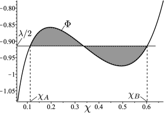
(a)		(b)

Figure 1: Local free energy and two coexisting states. (a) The local free energy $\int\Phi d\chi$ with $c=3.95$ and the two-points tangential line (dashed line) that determines the coexisting states. (b) The derivative of the local free energy $\Phi$ and the equi-area rule for determining the coexisting states, $\chi_{A}$ and $\chi_{B}$.

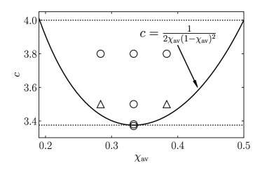
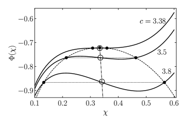
(a)		(b)

Figure 2: The neutral curve of linear stability and $\Phi(\chi)$ for different values of $c$. (a) The neutral curve (solid line) and the parameters of numerical simulations (open circles and triangles). (b) $\Phi(\chi)$ for $c=3.38$, $3.5$, and $3.8$. In (a), a uniform state is linearly unstable in the region above the neutral curve. In (b), the three points that are determined by the equi-area rule are indicated with a pair of closed circles and an open circle. The dashed and dot–dash lines are, respectively, the locus of the former and that of the latter in changing the value of $c$.

$$K\Delta\chi =\frac{1}{2}\ln\frac{\chi}{1-\chi}+\frac{1}{2}\frac{1}{1-\chi}-c\chi-\frac{1}{2}\lambda=\Phi(\chi)-\frac{1}{2}\lambda.$$ (59)

In one dimensional case, the above equation can be interpreted as a motion of point mass in a potential field $-\int\Phi(\chi)d\chi+(\lambda/2)\chi$ ($\chi$, $x$, and $K$ are interpreted as the position, time, and mass, respectively). This interpretation and following discussions in the present paragraph are due to van Kampen VK64 . Let us denote by $\chi_{A}$ and $\chi_{B}$ the values of $\chi$ at which a local maximum of the potential is achieved and thus the identity $\Phi(\chi_{A})=\Phi(\chi_{B})=\lambda/2$ ought to hold. This means that there is a common tangential line of $\int\Phi d\chi$ to $\chi=\chi_{A}$ and $\chi=\chi_{B}$, the slope of which is $\lambda/2$ [see figure 1(a)]. In the meantime, from a mechanical point of view, the potential height there should be the same in order for a spontaneous transition from one to the other to occur. Therefore $-\int^{\chi_{A}}\Phi(\chi)d\chi+(\lambda/2)\chi_{A}=-\int^{\chi_{B}}\Phi(\chi)d\chi+(\lambda/2)\chi_{B}$ or $\int_{\chi_{A}}^{\chi_{B}}\Phi d\chi=(\lambda/2)(\chi_{B}-\chi_{A})$. This implies that two shaded areas in figure 1(b) are the same (equi-area rule). Both interpretations, namely the common tangential line and the equi-area rule, often appear in the literature.

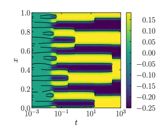
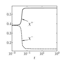
(a) $c=3.8$, $\chi_{\mathrm{av}}=23/60(=0.383)$
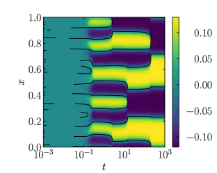
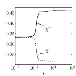
(b) $c=3.5$, $\chi_{\mathrm{av}}=1/3$
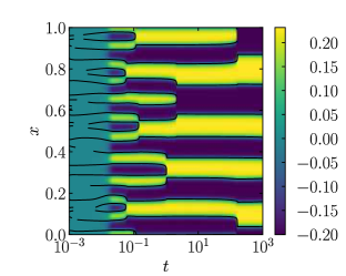
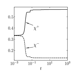
(c) $c=3.8$, $\chi_{\mathrm{av}}=1/3$

Figure 3: Phase transition towards two coexisting phases for various sets of parameters $(c,\chi_{\mathrm{av}})$, where $K$ is commonly set as $4.3976\times 10^{-5}$. In each case, the left panel shows the time evolution of dense (light-colored) and dilute (dark-colored) phases. The scale in the legend shows the deviation of $\chi$ from the average $\chi_{\mathrm{av}}$. The contour line of $\chi=\chi_{\mathrm{\mathrm{av}}}$ is drawn as well, but it is omitted where $|\partial\chi/\partial x|<0.05$ for the clarity of figure. The right panel shows the time evolution of the maximum/minimum values of $\chi$, say $\chi^{+}$ and $\chi^{-}$. From (a) to (e), the values of $k_{\mathrm{mr}}/2\pi$ are 10.3, 6.00, 11.1, 1.20, and 10.2. The corresponding number of regions is observed at the initiation of phase transition. The case (f) is in the range of linear stability and thus neither $k_{\mathrm{mr}}$ nor phase transition is found.

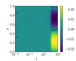
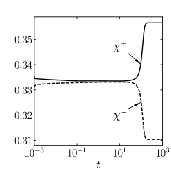
(d) $c=3.38$, $\chi_{\mathrm{av}}=1/3$
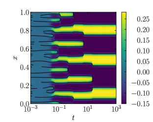
(e) $c=3.8$, $\chi_{\mathrm{av}}=17/60(=0.283)$
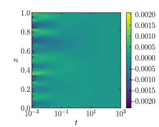
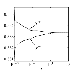
(f) $c=3.37$, $\chi_{\mathrm{av}}=1/3$

Figure 3: (continued from the previous page)

We now seek the condition that such different states can be found based on the present shape of the function $\Phi(\chi)$. Because

$$\Phi^{\prime}=\frac{1}{2}\frac{1}{\chi(1-\chi)^{2}}-c\equiv\frac{1}{2}\frac{1}{h(\chi)}-c,$$ (60)

and $h(\chi)$ takes its maximum $h_{\max}=4/27$ at $\chi=1/3$ and a common minimum $h_{\min}=0$ at $\chi=0,\ 1$. Hence, the condition $\Phi^{\prime}=0$ can be realized only when $c>27/8$. Furthermore, $c<4$ should be satisfied in order for the van der Waals equation of state (33) with $T=1$ to assure the positive pressure $p$ for any value of $\chi$. Therefore, we shall mainly study the case $27/8<c<4$ in the sequel.

6.3 Numerical simulations of the Cahn–Hilliard type equation

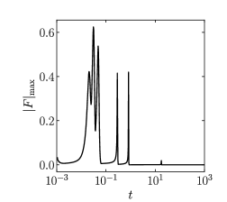
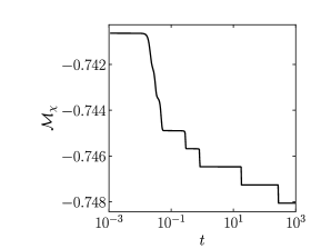
(a) $c=3.8$, $\chi_{\mathrm{av}}=23/60(=0.383)$
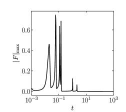
(b) $c=3.8$, $\chi_{\mathrm{av}}=1/3$
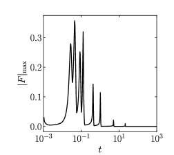
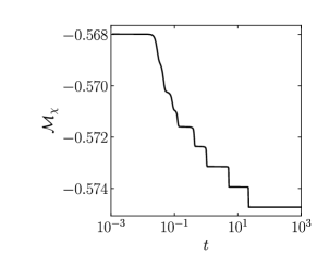
(c) $c=3.8$, $\chi_{\mathrm{av}}=17/60(=0.283)$

Figure 4: Time evolution of the maximum mass flux $|F|_{\max}$ and the functional $\mathcal{M}_{\chi}$.

We carried out numerical simulations of the Cahn–Hilliard type equation (52) for one-dimensional and two-dimensional cases for different parameter pairs of $c$ and $\chi_{\mathrm{av}}$. The chosen pairs are indicated by symbols in figure 2(a). For the parameter pairs indicated by open triangles, the results of two-dimensional simulations are just preliminary and will not be mentioned in the sequel. In all the simulations, another parameter $K$ is commonly set as $K=4.3976\times 10^{-5}$ and the uniform state with $\chi=\chi_{\mathrm{av}}$ is initially disturbed by a Gaussian random noise with the standard deviation of 0.001 (Further details of the initial disturbance can be found in Appendix B). The value of $K$ is chosen so that the most rapidly growing mode $k_{\mathrm{mr}}$ is about $6\times 2\pi$ in the case $(c,\chi_{\mathrm{av}})=(3.5,1/3)$.

We first show a part of the simulation results of one-dimensional simulations in figure 3. In each simulation, $\mathcal{M_{\chi}}$ was monitored, together with the maximum mass flux, i.e.,

$$|F|_{\max}=\max_{x\in D}|F|,\quad F\equiv-\chi\frac{\partial}{\partial x}(\Phi-K\frac{\partial^{2}\chi}{\partial x^{2}}).$$ (61)

Figure 4 shows the monitored results. In section 6.2, $\mathcal{M}_{\chi}$ has been evaluated under the assumption of the local equilibrium state $f=\rho E$. The assumption is, however, broken in the region where the mass flux is appreciable, as is clear in the analysis in section 6. In spite of this discrepancy, the results show the monotonic decrease of $\mathcal{M}_{\chi}$, which is consistent with the prediction in section 6.2. The resulting consistency can be understood if we recompute $\mathcal{M}$ (or $\mathcal{M}_{\chi}$) with a better approximation of $f$ , i.e.,

$$f=\rho E\{1-\frac{\varepsilon\zeta_{i}}{A(\rho)}\Big{(}\frac{1}{\rho}\frac{\partial\rho}{\partial x_{i}}+2\frac{\partial\phi}{\partial x_{i}}\Big{)}\}+o(\varepsilon).$$ (62)

Even with the refined $f$, we have

$$\langle f\ln\frac{f}{E}\rangle$$

$$\simeq\langle\rho E\{1-\frac{\varepsilon\zeta_{i}}{A(\rho)}\frac{\partial}{\partial x_{i}}\Big{(}\ln\rho+2\phi\Big{)}\}\ln[\rho\{1-\frac{\varepsilon\zeta_{i}}{A(\rho)}\frac{\partial}{\partial x_{i}}\Big{(}\ln\rho+2\phi\Big{)}\}]\rangle+o(\varepsilon)$$

$$\simeq\langle\rho E\{1-\frac{\varepsilon\zeta_{i}}{A(\rho)}\frac{\partial}{\partial x_{i}}\Big{(}\ln\rho+2\phi\Big{)}\}\{\ln\rho-\frac{\varepsilon\zeta_{i}}{A(\rho)}\frac{\partial}{\partial x_{i}}\Big{(}\ln\rho+2\phi\Big{)}\}\rangle+o(\varepsilon)$$

$$\simeq\langle\rho E\{1-\frac{\varepsilon\zeta_{i}}{A(\rho)}\frac{\partial}{\partial x_{i}}\Big{(}\ln\rho+2\phi\Big{)}\}\ln\rho-\rho E\frac{\varepsilon\zeta_{i}}{A(\rho)}\frac{\partial}{\partial x_{i}}\Big{(}\ln\rho+2\phi\Big{)}\rangle+o(\varepsilon)$$

$$\simeq\langle\rho E\ln\rho\rangle+o(\varepsilon)=\rho\ln\rho+o(\varepsilon).$$ (63)

Thus, $\mathcal{M}$ (or $\mathcal{M}_{\chi}$) remains unchanged up to $o(\varepsilon)$. Therefore, the deviation from the local Maxwellian $f=\rho E$, which mainly occurs at the interface, does not affect the minimization dynamics up to $o(\varepsilon)$. We therefore regard $\mathcal{M}_{\chi}$ as a functional to be minimized in time as well in the rest of the present subsection.

Now let us observe the results in figure 4 more closely. The above form of $F$ in (61) suggests that the flux is appreciable only at the interface. It is, however, appreciable only in more limited situations, namely the initiation of phase transition and subsequent emerging events of the same phases. Indeed, comparisons with the corresponding cases in figure 3 show a pulsive response of $|F|_{\mathrm{max}}$ to those limited situations. The functional $\mathcal{M}_{\chi}$ decreases monotonically, mostly with stepwise falls that synchronize the pulsive response of $|F|_{\mathrm{max}}$.

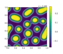
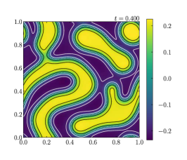
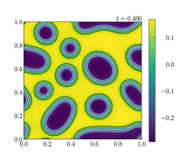
(a) $c=3.8$, $\chi_{\mathrm{av}}=17/60$	(b) $c=3.8$, $\chi_{\mathrm{av}}=1/3$	(c) $c=3.8$, $\chi_{\mathrm{av}}=23/60$

Figure 5: Contour plots of the rescaled density $\chi$ on the $xy$-plane: two coexisting phases at the instance $t=0.400$ induced by an Gaussian noise (with the standard deviation of 0.001) disturbance of an initial uniform state. The scale number in the legend indicates the value of $\chi-\chi_{\mathrm{av}}$. The contours are drawn with the interval of $0.1$. The contour of $\chi=\chi_{\mathrm{av}}$ is drawn by a dotted line, while other contours by solid lines.

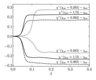
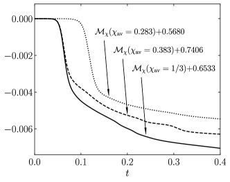
(a)		(b)

Figure 6: Time evolution of the maximum/minimum of $\chi$, say $\chi^{+}$ and $\chi^{-}$, and that of the system total free energy $\mathcal{M}_{\chi}$ in two dimensional cases. (a) $\chi^{\pm}$ vs. $t$ , (b) $\mathcal{M}_{\chi}$ vs. $t$ . Two parameters $K$ and $c$ are commonly set as $K=4.3976\times 10^{-5}$ and $c=3.8$, while the values of $\chi_{\mathrm{av}}$ are shown in the figure. The initial values of $\mathcal{M}_{\chi}$ are $-0.5680$, $-0.6533$, and $-0.7406$ for $\chi_{\mathrm{av}}=0.283(=17/60),$ $1/3$, and $0.383(=23/60)$, respectively.

In the two dimensional case, we observe a different feature of interface dynamics, which is absent in the one dimensional case and thus can be attributed to a multi-dimension effect; see figure 5. That is, depending on the average $\chi_{\mathrm{av}}$, the formation of interface geometry changes in quality. When $\chi_{\mathrm{av}}$ is high (low), the regions of dilute (dense) phase appear rather separately; and occasionally connected dilute (dense) regions change their shape toward circular discs. When $\chi_{\mathrm{av}}$ is intermediate, the interface keeps connected and accordingly its geometry remains complicated. Figure 6 shows the time evolution of the maximum/minimum of $\chi$ and $\mathcal{M}_{\chi}$. By comparing figures 6(a) and (b), the main decrease (or first drop) of $\mathcal{M}_{\chi}$ looks triggered by the first occurrence of phase transition. $\chi^{\pm}$ are almost saturated during the subsequent gradual decrease of $\mathcal{M}_{\chi}$. The gradual decrease of $\mathcal{M}_{\chi}$ looks attributed to a gradual deformation of the interface.

As to the details of the present numerical computations, the reader is referred to Appendix B.

7 Concluding remark

In the present paper, we presented a simple kinetic model for the phase transition of the van der Waals fluid. We constructed the model as simple as possible with retaining the essential features for reproducing the phase transition phenomenon. Although our model is rather primitive, it is reasonable enough to retain a firm connection to fluid dynamical and statistical mechanical concepts available in the literature. The simple role of the collision term as a thermal bath makes it easier to find the monotonically decreasing functional in time by the H theorem and its relation to the free energy in thermodynamics. The numerical simulations were conducted as well for the Cahn–Hilliard type equation that was obtained in the continuum limit of the presented model. The simulations demonstrated the actual occurrence of phase transition with this model and provided some details of dynamics in the near equilibrium regime.

As was briefly mentioned, we shall extend the present model to be applicable to far out of equilibrium gas flows. In such flows, the isothermal approximation is no longer appropriate and the contact with external walls is common. The extensions in these directions are not straightforward and are left for future works.

Appendix A Derivations of some equations

The equalities (20) and (21) are obtained as follows. First, the integration by part results in (20):

$$\int_{D}\rho v_{i}\frac{\partial\Phi_{L}}{\partial X_{i}}d\bm{X}=\int_{D}\frac{\partial}{\partial X_{i}}(\rho v_{i}\Phi_{L})d\bm{X}-\int_{D}\frac{\partial\rho v_{i}}{\partial X_{i}}\Phi_{L}d\bm{X}=\int_{D}\frac{\partial\rho}{\partial t}\Phi_{L}d\bm{X},$$ (64)

because at the second equality the first term vanishes by the periodic condition and the second term is transformed into the term on the right-hand side by using (7a). Next, using the definition of $\Phi_{L}$ [see (2)], the right-hand side of the above equation is transformed as

$$\int_{D}\frac{\partial\rho}{\partial t}\Phi_{L}d\bm{X}= \frac{1}{m}\int_{D}d\bm{X}\frac{\partial\rho(\bm{X})}{\partial t}\int_{\mathbb{R}^{3}}d\bm{r}\,\Psi(|\bm{r}|)\{\rho(\bm{X}+\bm{r})-\rho(\bm{X})\}$$

$$= \frac{1}{m}\frac{d}{dt}\int_{D}d\bm{X}\int_{\mathbb{R}^{3}}d\bm{s}\,\rho(\bm{X})\Psi(|\bm{X}-\bm{s}|)\{\rho(\bm{s})-\rho(\bm{X})\}$$

$$-\frac{1}{m}\int_{D}d\bm{X}\int_{\mathbb{R}^{3}}d\bm{s}\,\rho(\bm{X})\Psi(|\bm{X}-\bm{s}|)\frac{\partial}{\partial t}\{\rho(\bm{s})-\rho(\bm{X})\}$$

$$= \frac{1}{m}\frac{d}{dt}\int_{D}d\bm{X}\int_{\mathbb{R}^{3}}d\bm{s}\,\rho(\bm{X})\Psi(|\bm{X}-\bm{s}|)\{\rho(\bm{s})-\rho(\bm{X})\}$$

$$-\frac{1}{m}\int_{D}d\bm{s}\int_{\mathbb{R}^{3}}d\bm{X}\,\rho(\bm{X})\Psi(|\bm{X}-\bm{s}|)\frac{\partial}{\partial t}\rho(\bm{s})$$

$$+\frac{1}{m}\int_{D}d\bm{X}\int_{\mathbb{R}^{3}}d\bm{s}\,\rho(\bm{X})\Psi(|\bm{X}-\bm{s}|)\frac{\partial}{\partial t}\rho(\bm{X})$$

$$= \frac{1}{m}\frac{d}{dt}\int_{D}d\bm{X}\int_{\mathbb{R}^{3}}d\bm{s}\,\rho(\bm{X})\Psi(|\bm{X}-\bm{s}|)\{\rho(\bm{s})-\rho(\bm{X})\}$$

$$-\frac{1}{m}\int_{D}d\bm{X}\int_{\mathbb{R}^{3}}d\bm{s}\,\rho(\bm{s})\Psi(|\bm{X}-\bm{s}|)\frac{\partial}{\partial t}\rho(\bm{X})$$

$$+\frac{1}{m}\int_{D}d\bm{X}\int_{\mathbb{R}^{3}}d\bm{s}\,\rho(\bm{X})\Psi(|\bm{X}-\bm{s}|)\frac{\partial}{\partial t}\rho(\bm{X})$$

$$= \frac{1}{m}\frac{d}{dt}\int_{D}d\bm{X}\int_{\mathbb{R}^{3}}d\bm{s}\,\rho(\bm{X})\Psi(|\bm{X}-\bm{s}|)\{\rho(\bm{s})-\rho(\bm{X})\}$$

$$-\frac{1}{m}\int_{D}d\bm{X}\frac{\partial\rho(\bm{X})}{\partial t}\int_{\mathbb{R}^{3}}d\bm{s}\,\Psi(|\bm{X}-\bm{s}|)\{\rho(\bm{s})-\rho(\bm{X})\}$$

$$= \frac{d}{dt}\int_{D}\rho\Phi_{L}d\bm{X}-\int_{D}\frac{\partial\rho}{\partial t}\Phi_{L}d\bm{X}.$$ (65)

Here, we have suppressed $t$ in the arguments of $\rho$ for brevity. In the second term just after the third equality, the ranges of integration with respect to $\bm{X}$ and $\bm{s}$ have been interchanged by using the periodicity in space.

The above derivation of (21) relies on the specific form of $\Phi_{L}[\rho]$. However, we can show that (21) is valid as well when $\Phi_{L}=-\kappa\Delta\rho$. We omit its calculation here.

The reduction of $\mathcal{M}$ into the form (26) is carried out as follows.

$$\mathcal{M}(t) \equiv\int_{D}\{\langle f\ln\frac{f}{c_{0}}\rangle+\rho\ln(\frac{T^{3/2}}{T_{*}^{3/2}}\frac{\rho_{0}}{\rho})+\frac{\rho}{RT_{*}}(\mathcal{A}+\frac{1}{2}\bm{v}^{2}+\frac{1}{2}\Phi_{L})\}d\bm{X}$$

$$=\int_{D}\{\langle f\ln\frac{f}{c_{0}}\rangle+\frac{1}{RT_{*}}(\frac{1}{2}\langle\bm{c}^{2}f\rangle+\frac{1}{2}\rho\bm{v}^{2}+\int\Phi_{S}d\rho)+\frac{\rho}{2RT_{*}}\Phi_{L}[\rho]\}d\bm{X}$$

$$=\int_{D}\{\langle f\ln\frac{f}{c_{0}}\rangle+\frac{1}{RT_{*}}(\frac{1}{2}\langle\bm{\xi}^{2}f\rangle+\int\Phi_{S}d\rho)+\frac{\rho}{2RT_{*}}\Phi_{L}[\rho]\}d\bm{X}$$

$$=\int_{D}\{\langle f\ln\frac{f}{\rho_{0}M_{*}}\rangle+\frac{1}{RT_{*}}\int\Phi_{S}d\rho+\frac{\rho}{2RT_{*}}\Phi_{L}[\rho]\}d\bm{X}.$$ (66)

In the above transformation, there are two keys: one is the elimination of $\mathcal{A}$ from the expression by using (16), and the other is the relation $\langle\bm{\xi}^{2}f\rangle\propto\langle f\ln(\rho_{0}M_{*}/c_{0})\rangle$.

The second approximation to $g$, namely (46), is obtained by setting $f=f_{0}+g_{1}$ in (40). The process of transformation is as follows.

$$g_{2}= -\varepsilon(\mathrm{Sh}\frac{\partial f_{0}}{\partial t}+\zeta_{i}\frac{\partial f_{0}}{\partial x_{i}}-\frac{\partial\phi}{\partial x_{i}}\frac{\partial f_{0}}{\partial\zeta_{i}})\frac{1}{A(\rho)}-\varepsilon(\mathrm{Sh}\frac{\partial g_{1}}{\partial t}+\zeta_{i}\frac{\partial g_{1}}{\partial x_{i}}-\frac{\partial\phi}{\partial x_{i}}\frac{\partial g_{1}}{\partial\zeta_{i}})\frac{1}{A(\rho)}$$

$$= \,g_{1}+\varepsilon^{2}(\zeta_{i}\frac{\partial}{\partial x_{i}}-\frac{\partial\phi}{\partial x_{i}}\frac{\partial}{\partial\zeta_{i}})\{\zeta_{j}\frac{\rho E}{A(\rho)}\frac{\partial}{\partial x_{j}}(\ln\rho+2\phi)\}+o(\varepsilon^{2})$$

$$= -\varepsilon\{\mathrm{Sh}\frac{\partial\rho}{\partial t}+\zeta_{i}\rho\frac{\partial}{\partial x_{i}}(\ln\rho+2\phi)\}\frac{E}{A(\rho)}+\varepsilon^{2}\{\frac{\partial}{\partial x_{i}}\{\frac{\rho}{A(\rho)}\frac{\partial}{\partial x_{j}}(\ln\rho+2\phi)\}\}\zeta_{i}\zeta_{j}E$$

$$+\varepsilon^{2}2\rho\frac{\partial\phi}{\partial x_{i}}\frac{\partial}{\partial x_{j}}(\ln\rho+2\phi)(\zeta_{i}\zeta_{j}-\frac{1}{2}\delta_{ij})E\frac{1}{A(\rho)}+o(\varepsilon^{2})$$

$$= -\varepsilon\frac{\rho}{A(\rho)}\frac{\partial}{\partial x_{i}}(\ln\rho+2\phi)\zeta_{i}E+\frac{\varepsilon^{2}}{A(\rho)}\Big{\{}\frac{\partial}{\partial x_{i}}\{\frac{\rho}{A(\rho)}\frac{\partial}{\partial x_{j}}(\ln\rho+2\phi)\}$$

$$+\frac{2\rho}{A(\rho)}\frac{\partial\phi}{\partial x_{i}}\frac{\partial}{\partial x_{j}}(\ln\rho+2\phi)\Big{\}}(\zeta_{i}\zeta_{j}-\frac{1}{2}\delta_{ij})E+o(\varepsilon^{2}),$$ (67)

where (45) has been taken into account at the fourth equality.

Finally, the final form of (18) is the consequence of the following transformation.

$$\langle(1+\ln\frac{f}{\rho_{0}M_{*}})(\frac{\partial f}{\partial t}+\xi_{i}\frac{\partial f}{\partial X_{i}}+F_{i}\frac{\partial f}{\partial\xi_{i}})\rangle$$

$$= \frac{\partial}{\partial t}\langle f\ln\frac{f}{c_{0}}\rangle+\frac{\partial}{\partial X_{i}}\langle\xi_{i}f\ln\frac{f}{c_{0}}\rangle+\frac{1}{2RT_{*}}\langle\xi^{2}(\frac{\partial f}{\partial t}+\xi_{i}\frac{\partial f}{\partial X_{i}}+F_{i}\frac{\partial f}{\partial\xi_{i}})\rangle$$

$$= \frac{\partial}{\partial t}\langle f\ln\frac{f}{c_{0}}\rangle+\frac{\partial}{\partial X_{i}}\langle\xi_{i}f\ln\frac{f}{c_{0}}\rangle+\frac{1}{RT_{*}}\Big{\{}\frac{\partial}{\partial t}(\frac{1}{2}\langle\bm{c}^{2}f\rangle+\frac{1}{2}\rho v^{2}+\int\Phi_{S}d\rho)+\frac{\partial}{\partial x_{i}}\{(\frac{1}{2}\langle\bm{c}^{2}f\rangle$$

$$+\frac{1}{2}\rho v^{2}+\int\Phi_{S}d\rho)v_{i}+\frac{1}{2}\langle c_{i}\bm{c}^{2}f\rangle+(\langle c_{i}c_{j}f\rangle+\int\rho\Phi_{S}^{\prime}d\rho\delta_{ij})v_{j}\}\Big{\}}+\frac{\rho v_{i}}{RT_{*}}\frac{\partial\Phi_{L}}{\partial x_{i}}$$

$$= \frac{\partial}{\partial t}\Big{\{}\langle f\ln\frac{f}{c_{0}}\rangle+\frac{\rho}{RT_{*}}\{\frac{1}{2}v^{2}+\mathcal{A}+RT_{*}\ln(\frac{T^{3/2}}{T_{*}^{3/2}}\frac{\rho_{0}}{\rho})\}\Big{\}}+\frac{\partial}{\partial X_{i}}\Big{\{}\langle\xi_{i}f\ln\frac{f}{c_{0}}\rangle$$

$$+\frac{1}{RT_{*}}\{\rho v_{i}[\frac{1}{2}v^{2}+\mathcal{A}+RT_{*}\ln(\frac{T^{3/2}}{T_{*}^{3/2}}\frac{\rho_{0}}{\rho})]+\frac{1}{2}\langle c_{i}\bm{c}^{2}f\rangle+p_{ij}v_{j}\}\Big{\}}+\frac{\rho v_{i}}{RT_{*}}\frac{\partial\Phi_{L}}{\partial x_{i}}$$

$$= \frac{\partial}{\partial t}\{\langle f\ln\frac{f}{c_{0}}\rangle+\rho\ln(\frac{T^{3/2}}{T_{*}^{3/2}}\frac{\rho_{0}}{\rho})+\frac{\rho}{RT_{*}}(\mathcal{A}+\frac{1}{2}v^{2})\}+\frac{\partial}{\partial X_{i}}\Big{\{}\langle\xi_{i}f\ln\frac{f}{c_{0}}\rangle$$

$$+\rho v_{i}\ln(\frac{T^{3/2}}{T_{*}^{3/2}}\frac{\rho_{0}}{\rho})+\frac{1}{RT_{*}}\{\rho(\mathcal{A}+\frac{1}{2}v^{2})v_{i}+\frac{1}{2}\langle c_{i}\bm{c}^{2}f\rangle+p_{ij}v_{j}\}\Big{\}}+\frac{\rho v_{i}}{RT_{*}}\frac{\partial\Phi_{L}}{\partial x_{i}},$$ (68)

where $c_{0}=\rho_{0}(2\pi RT_{*})^{-3/2}$ and (7a) has been taken into account.

Appendix B Some details of the numerical computations

The original system is first discretized uniformly in each direction of space, where the second order central difference is adopted. To be more precise, the equation (52) is discretized in space as

$$\frac{\partial\chi}{\partial t}(x) =\delta_{h}[\chi(\tilde{x})\Phi^{\prime}(\chi(\tilde{x}))\delta_{h}[\chi](\tilde{x})-K\chi(\tilde{x})\delta_{h}^{3}[\chi](\tilde{x})](x),$$ (69a)

$$\delta_{h}[f](x)\equiv\frac{f(x+h)-f(x-h)}{2h},$$ (69b)

$$\delta_{h}^{3}[f](x)\equiv\frac{f(x+2h)-2f(x+h)+2f(x-h)-f(x-2h)}{2h^{3}},$$ (69c)

for one-dimensional (1D) simulations, while

$$\frac{\partial\chi}{\partial t}(x,y)= \Phi^{\prime}(\chi(x,y))\Big{\{}\{\delta_{hx}[\chi](x,y)\}^{2}+\{\delta_{hy}[\chi](x,y)\}^{2}+\chi(x,y)\delta_{h}^{2}[\chi](x,y)\Big{\}}$$

$$+\Phi^{\prime\prime}(\chi(x,y))\chi(x,y)\Big{\{}\{\delta_{hx}[\chi](x,y)\}^{2}+\{\delta_{hy}[\chi](x,y)\}^{2}\Big{\}}$$

$$-K\delta_{h}^{2}[\delta_{h}^{2}[\chi](\tilde{x},\tilde{y})](x,y),$$ (70a)

$$\delta_{hx}[f](x,y)\equiv\frac{f(x+h,y)-f(x-h,y)}{2h},$$ (70b)

$$\delta_{hy}[f](x,y)\equiv\frac{f(x,y+h)-f(x,y-h)}{2h},$$ (70c)

$$\delta_{h}^{2}[f](x,y)\equiv\frac{f(x+h,y)-2f(x,y)+f(x-h,y)}{h^{2}}$$

$$\qquad\qquad\qquad+\frac{f(x,y+h)-2f(x,y)+f(x,y-h)}{h^{2}},$$ (70d)

for two-dimensional (2D) simulations. Here $h$ is the interval of the uniform grid and $t$ has been suppressed in the argument of functions. In the standard grid system, the spatial domain is divided into 800 uniform intervals in each direction. All the results shown in section 6.3 are those obtained by the computations with the standard grid. As is already mentioned in section 6.3, the initial disturbance for each simulation is commonly a Gaussian noise with the standard deviation of $0.001$, but it is shifted in amplitude so as not to change the total mass in the domain. Furthermore, the Gaussian noise was generated on the basis of 100 grid for 1D and $100\times 100$ grid for 2D simulations so as not to change the initial disturbance for different grid systems. The minimum length of the generated randomness is eight-times longer than the interval of the standard grid ($800$ for 1D and $800\times 800$ for 2 D) in each spatial direction. This rather artificial care enables us to check the grid convergence of the numerical solutions, with keeping the randomness of the initial disturbance.

The time integration of the discretized system for 1D has been carried out by implementing the double-precision version of LSODA code in the ODEPACK developed by the Lawrence Livermore National Laboratory, which is available from http://www.netlib.org/odepack/ as of August 22, 2017. The code uses the Adams (predictor-corrector) method in the nonstiff case and the Backward Differentiation Formula (BDF) method in the stiff case, and it is decided adaptively which method to use. Actually, however, the Adams method was used only at the first time step in all of our simulations. The code uses both the variable timestep and the multistep, and the size of timestep and the degree of multistep (up to four steps) are optimized automatically as well. For the details of related optimization principle and features of LSODA itself, the reader is referred to HNW87 , as well as the summary text “odkd-sum” in the ODEPACK.

In the meantime, the time integration of the discretized system for 2D has been carried out by the explicit two-steps Runge–Kutta method, which is of the second order accuracy. If we symbolically rewrite (70) as $\partial\chi/\partial t=F(\chi)$, the time integration has been carried out by the following set of the prediction and correction steps

$$\tilde{\chi}_{n+1}=\chi_{n}+F(\chi_{n})\Delta t_{n+1},$$ (71a)

$$\chi_{n+1}=\chi_{n}+\frac{1}{2}\{F(\chi_{n})+F(\tilde{\chi}_{n+1})\}\Delta t_{n+1},$$ (71b)

where $\chi_{n}$ denotes the value of $\chi$ at $t=t_{n}$ ($t_{0}=0$) and $\Delta t_{n+1}=t_{n+1}-t_{n}$. The correction step is taken only once in a single time step, namely the so-called PEC mode is adopted. The timestep $\Delta t_{n+1}$ is fixed, in contrast to 1D simulations, as $1\times 10^{-9}$ for the standard grid ($800\times 800$), $2\times 10^{-8}$ for $400\times 400$ grid, $2\times 10^{-7}$ for $200\times 200$ grid, and $2\times 10^{-6}$ for $100\times 100$ grid.

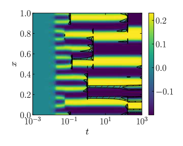
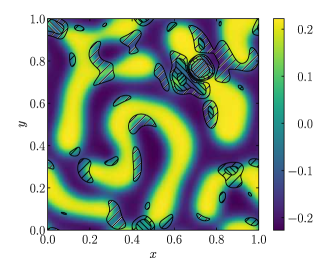
(a) 1D	(b) 2D

Figure 7: Grid dependence of the results for the case $c=3.8$, $\chi_{\mathrm{av}}=1/3$, and $K=4.3976\times 10^{-5}$. (a) The difference $\Delta$ between the results with standard and double-size coarse grids in the 1D simulation. (b) The difference $\Delta$ at $t=0.2$ between the results with standard and double-size coarse grids in the 2D simulation. The three types of hatched area, namely the upward hatched area with wide interval, the downward hatched area, and the upward hatched area with narrow interval, represent the area where $0.003<\Delta<0.01$, $0.01<\Delta<0.03$, and $0.03<\Delta$. The scale in the legend shows $\chi-\chi_{\mathrm{av}}$.

We implemented the LSODA code as well for the time integration in 2D. However, it turned out to be very time consuming and had to be limited only to four- or more-times coarse grids. For the four- or more-times coarse grids, we had a reasonable agreement between the results of Runge-Kutta and LSODA codes.

The present scheme for both 1D and 2D is not based on a mass preserving method. Nevertheless, we observed that the total mass was perfectly preserved in 1D simulations. In contrast, in 2D simulations, a straightforward implementation caused a gradual change of the total mass in the domain in both the Runge-Kutta and LSODA codes, which could affect the main feature of the phase transition in the system. We therefore renormalize the total mass at the beginning of every time step. The adverse side effect of this remedy should be carefully assessed. We thus performed the simulations without renormalization for the same grid and those with renormalization for a more refined grid as well. The multiplied factor for the renormalization was close to unity, the deviation from which was about $1.47\times 10^{-11}$ for the standard grid ($800\times 800$), $5.50\times 10^{-10}$ for $400\times 400$ grid, and $2.15\times 10^{-8}$ for $200\times 200$ grid. The size of deviations per unit time was decreasing from $0.10$ (for $200\times 200$ grid) to $0.028$ or $0.015$ (for $400\times 400$ or $800\times 800$ grid), showing the improvement of reliability by a grid refinement. We did not find any qualitative difference among the above three types of simulations, such as the spatial arrangement of different phases, the number of the dilute/dense regions. However, due to slight differences of the instance of merging and of the interface position, the grid dependence of $\chi$ at a fixed position and time is not necessarily small, see figure 7. All the numerical results presented in section 6.3 are those obtained with the standard grid and with the remedy of total mass renormalization.

References

• (1) S. Chapman and T.G. Cowling, The Mathematical Theory of Non-uniform Gases, 3rd ed. (Cambridge University Press, Cambridge, 1995), Chap. 16.
• (2) J.O. Hirschfelder, C.F. Curtiss, and R.B. Bird, The Molecular Theory of Gases and Liquids (Wiley, New York, 1964), Sec. 9.3.
• (3) M. Grmela, J. Stat. Phys. 3, 347 (1971).
• (4) A. Frezzotti, L. Gibelli, and S. Lorenzani, Phys. Fluids 17 012102 (2005).
• (5) K. Kobayashi, K. Ohashi, and M. Watanabe, AIP Conference Proceedings 1501, 1145 (2012).
• (6) A. Frezzotti and P. Barbante, Mech. Eng. Reviews 4, 16-00540 (2017).
• (7) M.R. Swift, E. Orlandini, W.R. Osborn, and J.M. Yeomans, Phys. Rev. E 54, 5041 (1996).
• (8) G. Gonnella, A. Lamura, and V. Sofonea, Phys. Rev. E 76, 036703 (2007).
• (9) J.S. Rowlinson and B. Widom, Molecular Theory of Capillarity (Dover, New York, 2002), Sec. 1.4 and Chap. 3.
• (10) E.A. Carlen, M.C. Carvalho, R. Esposito, J.L. Lebowitz, and R. Marra, Molecular Physics 103, 3141 (2005).
• (11) N.G. van Kampen, Phy. Rev. 135, A362 (1964).
• (12) E. Hairer, S.P. Norsett, G. Wanner, Solving Ordinary Differential Equations I (Springer-Verlag, Berlin, 1987), Chap. III.