Measurement of Total and Differential Cross Sections of Neutrino and Antineutrino Coherent $\pi^{\pm}$ Production on Carbon

Abstract

Neutrino induced coherent charged pion production on nuclei, $\overline{\nu}_{\mu}A\to\mu^{\pm}\pi^{\mp}A$, is a rare inelastic interaction in which the four-momentum squared transfered to the nucleus is nearly zero, leaving it intact. We identify such events in the scintillator of MINERvA by reconstructing $|t|$ from the final state pion and muon momenta and by removing events with evidence of energetic nuclear recoil or production of other final state particles. We measure the total neutrino and antineutrino cross sections as a function of neutrino energy between 2 and 20 GeV and measure flux integrated differential cross sections as a function of $Q^{2}$, $E_{\pi}$ and $\theta_{\pi}$. The $Q^{2}$ dependence and equality of the neutrino and anti-neutrino cross-sections at finite $Q^{2}$ provide a confirmation of Adler’s PCAC hypothesis.

I Introduction

Neutrino-nucleus coherent pion production is an inelastic interaction that produces a lepton and a pion in the forward direction while leaving the nucleus in its initial state. The charged current (CC) processes are

$$\nu_{l}+\text{A}\to l^{-}+\pi^{+}+\text{A}$$

$$\overline{\nu}_{l}+\text{A}\to l^{+}+\pi^{-}+\text{A}$$ (1)

and the neutral current (NC) processes are

$$\nu_{l}+\text{A}\to\nu_{l}+\pi^{0}+\text{A}$$

$$\overline{\nu}_{l}+\text{A}\to\overline{\nu}_{l}+\pi^{0}+\text{A}$$ (2)

where A is the nucleus. For the interaction to preserve the initial state of the nucleus, the absolute value of the square of the four-momentum exchanged with the nucleus, $|t|$, must be small. In addition, the particle(s) exchanged with the nucleus can only carry vacuum quantum numbers in coherent scattering.

Coherent pion production is not a common process; for neutrino (antineutrino) interactions on carbon nuclei at $E_{\nu}\sim$3 GeV, theoretical models (see Sec. VI) predict the rate of coherent pion production to be only $\sim$1% ($\sim$3%) of the total interaction rate for both CC and NC interactions. Nonetheless, coherent pion production is an important background for neutrino oscillation experiments, which typically operate in the range 1 GeV$\lesssim E_{\nu}\lesssim$ 10 GeV. NC coherent pion production is an important background to $\nu_{\mu}\to\nu_{e}$ and $\overline{\nu}_{\mu}\to\overline{\nu}_{e}$ oscillation measurements where the oscillation signals are $\nu_{e}+N\to e^{-}+X$ and $\overline{\nu}_{e}+N\to e^{+}+X$, where $N$ is a target nucleon and $X$ is the hadronic final state. NC coherent pion production yields only a $\pi^{0}$ to be observed in the detector and if one of the two final state photons is not observed, the other can be mistaken for an electron or positron. CC coherent pion production is a background to measurements of $\nu_{\mu}$ and $\overline{\nu}_{\mu}$ disappearance at low neutrino energy ($E_{\nu}\lesssim$ 1 GeV) where quasielastic scattering

$$\nu_{\mu}+n\to\mu^{-}+p$$

$$\overline{\nu}_{\mu}+p\to\mu^{+}+n$$ (3)

is the primary interaction process. Coherent pion production can be mistaken for quasielastic scattering when the $\pi^{\pm}$ is misidentified as a proton or is not detected.

This paper presents precise measurements of the $\nu_{\mu}$ and $\overline{\nu}_{\mu}$ CC coherent pion production cross sections on carbon for 2 $<E_{\nu}<$ 20 GeV. The cross sections are measured as a function of the pion energy, pion angle, and $Q^{2}$, which characterize the coherent pion production kinematics. A subset of these results based on this same data was published earlier bib:minerva_coh . The results presented in this paper have a revised treatment of backgrounds, additional differential distributions, a new prediction of the neutrino and antineutrino fluxes in the beam and the correlations between the neutrino and antineutrino measurements. Also presented is a study from the data of the possible contributions of diffractive scattering to this measurement of coherent pion production. Accordingly, the results in this paper supersede those of Ref. bib:minerva_coh .

This paper is organized as follows. Sections II and III describe two existing models and the experimental state of the field prior to this work. Section IV introduces diffractive scattering of neutrinos off hydrogen, an important and closely related process that is studied here. Sections V-VIII describe the experiment, the event selection and the reconstruction of candidate events. Sections IX-XII explain the measurement of the cross sections and their systematic uncertainties. Sections XIII-XV present the results and their interpretation.

II Models

PCAC coherent models bib:coh_pcac3 ; bib:coh_pcac4 ; bib:coh_pcac5 ; bib:coh_pcac6 ; bib:coh_pcac7 ; bib:coh_pcac10 and bib:RS ; bib:RS2 ; bib:berger_sehgal ; bib:kartavtsev ; bib:manny are a class of coherent pion production models that are based on Adler’s PCAC theorem bib:adler_pcac (Partial Conservation of Axial Current, or in modern language, spontaneous breaking of chiral symmetry in QCD) which can be used to relate coherent pion production at $Q^{2}=-(p_{\nu}-p_{l})^{2}=0$ to elastic pion-nucleus scattering. Here, $p_{\nu}$ ($p_{l}$) is the four-momentum of the incoming neutrino (outgoing charged lepton). In this picture of coherent pion production, the intermediate weak boson fluctuates to a virtual pion, which scatters elastically off the nucleus, as shown in the Pomeron (IP) diagram of Fig. 1.

II.A Rein-Sehgal Model

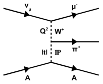
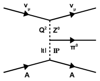
Figure 1: CC (left) and NC (right) neutrino-nucleus coherent pion production in the PCAC picture.

The Rein-Sehgal coherent model bib:RS ; bib:RS2 is the most widely used PCAC coherent pion production model in neutrino event generators. The Rein-Sehgal model extrapolates the Adler coherent cross section result to $Q^{2}>0$ using a multiplicative axial-vector dipole form factor

$$F_{A}=\frac{M_{A}^{2}}{Q^{2}+M_{A}^{2}},$$ (4)

where $M_{A}\approx$ 1 GeV is the axial vector mass. The Rein-Sehgal model assumes no vector current contribution in this extrapolation, and therefore predicts equal cross sections for neutrinos and antineutrinos.

The Rein-Sehgal model calculates the $\pi^{\pm}$A elastic cross section using charged pion-nucleon ($\pi^{\pm}N$) scattering data.

The differential CC coherent pion production cross section calculated by the Rein-Sehgal model is

$$\frac{d\sigma_{coh}^{CC}}{dQ^{2}dyd|t|} =\frac{G^{2}f_{\pi^{\pm}}^{2}}{2\pi}\frac{(1-y)}{y}\frac{M_{A}^{2}}{Q^{2}+M_{A}^{2}}A^{2}$$ (5)

$$\times\exp\left(-\frac{1}{3}R_{0}^{2}A^{2/3}|t|-\frac{9A^{1/3}}{16\pi R_{0}^{2}}\sigma_{inel}^{\pi^{\pm}N}(E_{\pi})\right)$$

$$\times\frac{1}{16\pi}\left(\sigma_{tot}^{\pi^{\pm}N}(E_{\pi})\right)^{2}(1+r^{2}),$$

where the pion energy $E_{\pi}=yE_{\nu}$, $A$ is the atomic number of the target nucleus, $f_{\pi}$ is the pion decay constant, $R_{0}$ is the nuclear length scale $\sim 1$ fm and $r=\text{Re}f(0)/\text{Im}f(0)$ is the ratio of the real and imaginary parts of the $\pi^{\pm}N$ forward scattering amplitude. The exponential dependence in $|t|$ is the consequence of a simple gaussian model for the nuclear form factor in $\pi A$ elastic scattering. The Rein-Sehgal model calculates the NC differential cross section from Eq. (5) using $f_{\pi^{0}}=f_{\pi^{\pm}}/\sqrt{2}$ and assuming that the $\pi^{\pm}N$ and $\pi^{0}N$ cross sections are equal.

The Rein-Sehgal model corrects the CC differential cross section (Eq. 5) for the mass of the final state lepton bib:RS2 ; bib:lepton_mass_corr . The correction, proposed by Adler bib:lepton_mass_corr , is

$$C =\left(1-\frac{1}{2}\frac{Q^{2}_{min}}{Q^{2}+m^{2}_{\pi}}\right)^{2}+\frac{y}{4}\frac{Q^{2}_{min}(Q^{2}-Q^{2}_{min})}{(Q^{2}+m^{2}_{\pi})^{2}}$$

$$\times\theta(Q^{2}-Q^{2}_{min})\theta(y-y_{min})\theta(y_{max}-y),$$

where $Q^{2}_{min}=m^{2}_{l}y/(1-y)$ is the kinematic minimum $Q^{2}$, $y_{min}=m_{\pi}/E_{\nu}$ and $y_{max}=1-m_{l}/E_{\nu}$ are the kinematic minimum and maximum $y$, and $m_{l}$ and $m_{\pi}$ are the final state lepton and pion masses.

The Rein-Sehgal model predicts that both $\sigma_{coh}^{CC}(E_{\nu})$ and $\sigma_{coh}^{NC}(E_{\nu})$ scale with $A$ approximately as $A^{1/3}$, as a result of the nuclear coherence condition and pion absorption effects.

II.B Berger-Sehgal Model

The cross section of Eq. (5) is differential in three variables but coherent scattering only occurs in a limited region of the phase space. Newer models bib:berger_sehgal ; bib:kartavtsev ; bib:manny use data from pion-nucleus elastic scattering. These show that coherent scattering predominantly occurs at $Q^{2}$ $\sim\mathcal{O}(m_{\pi}^{2}),~{}\nu^{2}=(E_{\nu}-E_{l})^{2}\gg Q^{2}$ and $|t|\lesssim 1/R^{2}$, where $E_{\nu}$ ($E_{l}$) is the energy of the incoming neutrino (outgoing lepton) and $R$ is the radius of the nucleus. In particular, coherent scattering creates a sharp increase in the slope of $d\sigma/d|t|$ as $|t|$ approaches $|t|_{min}$ $\sim\frac{(Q^{2}+m_{\pi}^{2})^{2}}{2\nu}$, the minimum kinematically possible $|t|$. The Berger-Sehgal PCAC coherent model bib:berger_sehgal is a modification of the Rein-Sehgal model where the parameterization of the $\pi^{\pm}$A elastic scattering cross section is instead fit to charged pion-carbon ($\pi^{\pm}$C) elastic scattering data and scaled to other nuclei. This approach avoids some of the uncertainties from modeling nuclear effects, e.g. pion absorption, in the Rein-Sehgal parameterization. In the Berger-Sehgal model, coherent cross sections scale as $A^{2/3}$. The comparison of Rein-Sehgal and Berger-Sehgal calculations of $\sigma_{el}^{\pi^{\pm}\text{C}}$ in Fig. 2 shows that while the two calculations agree for $|\vec{p}_{\pi}|\gtrsim 0.7$ GeV, the Rein-Sehgal predicts a much larger cross section in the $\Delta$ resonance dominated region, $|\vec{p}_{\pi}|\sim 0.3$ GeV.

Figure 2: The Rein-Sehgal (dashed line) and Berger-Sehgal (solid line) pion-carbon elastic scattering cross sections as a function of the pion momentum in the laboratory frame. From bib:berger_sehgal .

III Earlier Measurements

Coherent CC interactions can be identified by requiring that the observed final state consist only of a charged lepton and pion (the target nucleus is not observed since the energy transferred to the nucleus is small) and small $|t|$. From the assumption of zero energy transfer to the nucleus,

$$|t| =|(p_{\nu_{l}}-p_{l}-p_{\pi})^{2}|$$ (7)

$$\approx\left(\displaystyle\sum_{i=\mu,\pi}E_{i}-p_{i,L}\right)^{2}+\left|\displaystyle\sum_{i=\mu,\pi}\vec{p}_{i,T}\right|^{2},$$

where $p_{\nu_{l}}$, $p_{l}$, and $p_{\pi}$ are the four-momenta of the neutrino, charged lepton, and pion, respectively, and $\vec{p}_{T}$ and $p_{L}$ are transverse and longitudinal momenta with respect to the incoming neutrino direction. The neutrino four-momentum is determined by assuming that its direction is that of the neutrino beam and its energy is $E_{\nu}=E_{l}+E_{\pi}$.

For NC coherent interactions, the final state neutrino is not observed and the observed final state is a lone $\pi^{0}$. Neither $E_{\nu}$ nor $|t|$ can be measured. Since $|t|$ is not available, experiments isolate NC coherent interactions using the condition

$$E_{\pi}(1-\cos\theta_{\pi})<\frac{1}{R},$$ (8)

where $\theta_{\pi}$ is the angle between the pion and incoming neutrino directions. This condition follows from the $|t|\lesssim 1/R^{2}$ condition for coherent scattering at $Q^{2}\approx$ 0 bib:lackner . However, imposing selection requirements on the pion kinematics creates implicit selection requirements on the lepton kinematics and $Q^{2}$ (see Eq. 7). Consequently, NC coherent pion production measurements must make model-dependent assumptions about the $Q^{2}$ dependence of the coherent scattering cross section when correcting for the inefficiency of this selection requirement.

Since $E_{\nu}$ cannot be measured, NC coherent pion production measurements are averaged over the energy spectrum of a neutrino beam. These experimental limitations of NC coherent pion production measurements increase the importance of CC coherent pion production measurements, which in the PCAC picture provide a constraint on the NC reaction.

Many measurements of NC bib:coh_nc_AP ; bib:coh_nc_garg ; bib:coh_nc_charm ; bib:coh_nc_cc_skat ; bib:coh_nc_fnal ; bib:coh_nc_nomad ; bib:coh_nc_sb ; bib:coh_nc_mb ; bib:coh_nc_minos and CC bib:coh_nc_cc_skat ; bib:coh_cc_bebc1 ; bib:coh_cc_fnal1 ; bib:coh_cc_bebc2 ; bib:coh_cc_fnal2 ; bib:coh_cc_fnal3 ; bib:coh_cc_charm ; bib:coh_cc_k2k ; bib:coh_cc_sb ; bib:coh_cc_argo coherent pion production have been made at neutrino energies of 1 $\lesssim E_{\nu}\lesssim$ 100 GeV using both $\nu_{\mu}$ and $\overline{\nu}_{\mu}$ beams and a variety of scattering target materials (carbon, neon, aluminum, argon, Freon, glass, marble and iron). Measurements made before the discovery of neutrino oscillations were mostly made at $E_{\nu}>$ 10 GeV. Precise measurements at 1 $\lesssim E_{\nu}\lesssim$ 10 GeV are now needed for constraining backgrounds in oscillation measurements in high intensity $\nu_{\mu}$ and $\overline{\nu}_{\mu}$ beams.

Early measurements of the NC coherent pion production cross section as a function of $E_{\nu}$ bib:coh_nc_AP ; bib:coh_nc_garg ; bib:coh_nc_charm are shown in Fig. 3. They were made using different scattering target materials and, for the purpose of comparison, are scaled in Fig. 3 to a marble scattering target with an effective $A$ = 20 using the $A^{1/3}$ dependence of the cross section. While the Rein-Sehgal model prediction agrees with the measured cross sections within their uncertainties, the uncertainties are large ($\gtrsim$ 30% bib:coh_nc_nomad ).

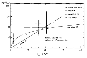
Figure 3: Early measurements of the NC coherent pion production cross section. The horizontal error bars represent the range of neutrino energies sampled by the measurement. The figure is from bib:coh_nc_charm .

Early measurements of the $\nu_{\mu}$ and $\overline{\nu}_{\mu}$ CC coherent pion production cross sections as a function of $E_{\nu}$ bib:coh_nc_cc_skat ; bib:coh_cc_bebc1 ; bib:coh_cc_fnal1 ; bib:coh_cc_bebc2 ; bib:coh_cc_fnal2 ; bib:coh_cc_fnal3 ; bib:coh_cc_charm , along with the early measurements of the NC coherent pion production cross section bib:coh_nc_AP ; bib:coh_nc_garg ; bib:coh_nc_charm ; bib:coh_nc_cc_skat , are shown in Fig. 4. For comparison, the measurements in Fig. 4 are scaled to a glass scattering target with an effective $A$ = 20.1, and the NC measurements are additionally scaled by a factor of 2 per the relation between the CC and NC coherent cross sections from Adler’s PCAC theorem. These early CC measurements isolated CC coherent interactions by requiring a forward $\mu^{\mp}$ and $\pi^{\pm}$, the absence of additional particles emerging from the interaction vertex, and small $|t|$. The Rein-Sehgal model agrees well with most of the measurements, which supports the predicted $A^{1/3}$ dependence and the 2-to-1 relationship between the CC and NC coherent cross sections.

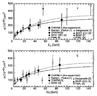
Figure 4: Early measurements of the $\nu_{\mu}$ (top) and $\overline{\nu}_{\mu}$ (bottom) CC coherent pion production cross sections. The solid line is the Rein-Sehgal model prediction. The figure is from bib:coh_cc_charm .

The only measurements of NC coherent pion production at $E_{\nu}<$ 2 GeV were made recently by the MiniBooNE bib:coh_nc_mb and SciBooNE bib:coh_nc_sb experiments. The MiniBooNE measurement was made using a mineral oil target (CH₂) at a peak $E_{\nu}$ of 0.7 GeV. MiniBooNE measured the NC coherent pion production cross section to be $(19.5\pm 2.7)$% of the total (coherent + non-coherent) NC single $\pi^{0}$ production cross section. The SciBooNE measurement was made using a polystyrene target (CH) at an average $E_{\nu}$ of 0.8 GeV. SciBooNE measured the ratio of the NC coherent pion production cross section to the $\nu_{\mu}$ CC total (all scattering processes) cross section to be $(1.16\pm 0.24)\times 10^{-2}$.

The first searches for $\nu_{\mu}$ CC coherent pion production at $E_{\nu}\lesssim$ 2 GeV were performed by the K2K bib:coh_cc_k2k and SciBooNE bib:coh_cc_sb experiments. These experiments used the same CH-based detector in two different neutrino beams. Neither could measure $|t|$ since the detector did not provide adequate containment of the pion to allow accurate measurement of the pion energy, and instead searched for coherent scattering at low $Q^{2}$. Neither experiment found evidence for CC coherent interactions after subtracting the predicted non-coherent background (Figs. 5 and 6). The experiments reported upper limits on the ratio of the $\nu_{\mu}$ CC coherent pion production cross section to the $\nu_{\mu}$ CC total cross section, which are listed in Table 1.

The non-observation of $\nu_{\mu}$ CC coherent pion production at $E_{\nu}<$ 2 GeV is in contradiction to the the Rein-Sehgal coherent model. It should be noted that a search for coherent pion production in $Q^{2}$ is model dependent. In addition, both the K2K and SciBooNE measurements constrained their background prediction using interactions with activity near the interaction vertex in addition to that from the muon and pion. The background prediction is therefore sensitive to the modeling of nuclear effects which are poorly understood (see Sec. IX).

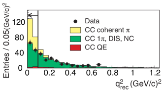
Figure 5: The data and simulated $Q^{2}$ distributions for $\nu_{\mu}$ CC coherent pion production candidates at K2K. The figure is from bib:coh_cc_k2k .

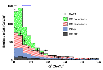
Figure 6: The data and simulated $Q^{2}$ distributions for $\nu_{\mu}$ CC coherent pion production candidates at SciBooNE. The figure is from bib:coh_cc_sb .

Experiment	$\sigma_{CC}^{coh}/\sigma_{CC}^{tot}$ (90% C.L.)	$\langle E_{\nu}\rangle$ (GeV)
K2K	$<$ 0.6 $\times$ 10-2	1.3
SciBooNE	$<$ 0.67 $\times$ 10-2	1.1
SciBooNE	$<$ 1.36 $\times$ 10-2	2.2

Table 1: The upper limits on the ratio of the $\nu_{\mu}$ CC coherent pion production cross section to the $\nu_{\mu}$ CC total cross section, $\sigma_{CC}^{coh}/\sigma_{CC}^{tot}$, reported by K2K bib:coh_cc_k2k and SciBooNE bib:coh_cc_sb .

The non-observation of CC coherent pion production at $E_{\nu}\lesssim$ 2 GeV posed a problem for both theorists and neutrino oscillation experiments; production models are unable to reconcile it with the observation of the NC reaction at the same $E_{\nu}$. To account for the theoretical and experimental disagreement, the T2K neutrino oscillation measurement, which operates at $E_{\nu}$ $\approx$ 0.6 GeV, applied a 100% uncertainty on their predicted CC coherent interaction rate, while applying a 30% uncertainty on their predicted NC coherent interaction rate bib:t2k_osc .

Precise measurements of neutrino-nucleus coherent pion production at 1 $\lesssim E_{\nu}\lesssim$ 10 GeV are needed for testing coherent pion production models and reducing systematic uncertainties in neutrino oscillation measurements.

IV Diffractive Scattering

Diffractive pion production, $\nu_{\mu}p\to\mu^{-}\pi^{+}p$ (Fig. 7) is a process similar to coherent scattering but for single proton. It produces a muon and charged pion in the forward direction while leaving the nucleus, i.e. the proton, intact and with minimal recoil. Like coherent scattering, diffractive production occurs at low $|t|$. Unlike coherent scattering, the recoil proton does absorb some kinetic energy, making it potentially visible in the detector. There are also resonant and non-resonant processes that occur in a broader range of $|t|$. At low $|t|$ these may interfere with the diffractive process which complicates the prediction of the process.

Diffractive scattering is experimentally indistinguishable from coherent scattering when the recoil proton is below detection threshold. A $\nu_{\mu}$/ $\overline{\nu}_{\mu}$ CC sample in the MINERvA tracker may contain diffractive scattering interactions since the CH scintillator contains free protons. Diffractive scattering was not included in the simulated backgrounds to the coherent process, so the measured coherent cross section may therefore contain a contribution from it. It is not coherent scattering on carbon and is therefore a potential background to this measurement. One of the new results presented here is that in fact this potential background has a rate consistent with zero.

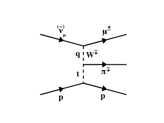
Figure 7: Diffractive pion production on a free proton.

An important difference between coherent and diffractive scattering is the $|t|$-dependence of the cross sections. In the PCAC picture of diffractive scattering, the intermediate weak boson fluctuates to a pion, which scatters elastically off the target proton. The expectation therefore is that the $|t|$-dependence comes from the pion-proton/nucleus elastic scattering cross section, which is assumed to fall exponentially with $|t|$ as $\exp(-b|t|)$ for the same reason that it is a reasonable choice in the Rein-Sehgal model of coherent scattering bib:RS . The exponential slope $b$ is given by

$$b=\frac{1}{3}R_{0}^{2}A^{2/3},$$ (9)

where $R_{0}\sim$1 fm is the nuclear length scale and A is the number of nucleons in the target. The predicted exponential slope for coherent scattering on carbon ($A=12$) is $\sim$40 (GeV/c)^-2, and the predicted exponential slope for diffractive scattering ($A=1$) is $\sim$8 (GeV/c)^-2. The diffractive cross section therefore falls more slowly with $|t|$ than the coherent cross section. The squared four-momentum exchanged with the target proton in diffractive scattering $|t|_{diff}$ is related to the recoil proton kinetic energy $T_{p}$ by

$$|t|_{diff} =|(p_{\nu}-p_{\mu}-p_{\pi})^{2}|$$ (10)

$$=|(p_{p,f}-p_{p,i})^{2}|=2m_{p}T_{p},$$

where $p_{\nu}$ is the neutrino four-momentum, $p_{\mu}$ is the muon four-momentum, $p_{\pi}$ is the pion four-momentum, $p_{p,i}$ and $p_{p,f}$ are the target (initial state) and recoil (final state) proton four-momentum and $m_{p}$ is the proton mass. The target proton is assumed to be on-shell and at rest. The amount of energy deposited in the detector by the recoil proton in a diffractive scattering interaction determines whether the interaction is accepted or rejected by the vertex energy cut (Sec.  VIII.E) which requires that energy near the interaction vertex is consistent with the energy deposited by only a muon and a pion. Accepted events are therefore restricted to small $T_{p}$, and equivalently small $|t|$. The small $|t|$ diffractive acceptance in conjunction with the slowly falling $|t|$-dependence of the diffractive cross section results in a small contribution of diffractive scattering to the measured coherent cross sections.

Predictions for the diffractive pion production and the possible contribution to the signal sample are discussed in Sec. XI.

V Neutrino Beam and Detector

The MINERvA experiment is in the NuMI beamline at Fermilab. Both the beamline and detector are described in detail elsewhere bib:numi_beam ; bib:minerva_nim ; here is a short summary.

A beam of 120 GeV protons strikes a graphite target, and the charged mesons produced there are focused by two magnetic horns into a helium-filled decay pipe 675 m long. The horns focus positive (negative) mesons, resulting in a $\nu_{\mu}$ ($\overline{\nu}_{\mu}$) enriched beam with a peak neutrino energy of 3.5 GeV. Muons produced in meson decays are absorbed in the 240 m of rock downstream of the decay pipe. The neutrino beam is simulated in a Geant4-based bib:geant1 model weighted to reproduce hadron production measurements bib:flux .

Roughly $85\%$ of the neutrinos are produced by interactions of protons on carbon, and data from the NA49 and Barton et. al. experiments bib:na49 ; bib:barton is used to constrain the production of the charged pions and kaons that decay to neutrinos. Proton interaction rates with aluminum, iron, and helium nuclei were tuned to the $pC$ data using an $A$-dependent scaling; neutron interaction rates with carbon were also tuned to the $pC$ data using isospin symmetry. Rates for interactions where there are no applicable measurements were taken from the hadron interaction model used in the simulation (FTFP-BERT). Predictions from the weighted model were compared against in-situ measurements of neutrino scattering events with low hadronic recoil to validate the model. An in situ measurement bib:veve of $\nu+e^{-}\rightarrow e^{-}+\nu$ provided an additional constraint on the flux, giving a roughly 2-4 % reduction in the flux prediction and an $\sim$ 1 % reduction in the flux uncertainty. The uncertainty in the prediction of the neutrino flux, discussed in more detail later, is set by (a) the precision in these hadron production measurements, (b) uncertainties in the beam line focusing system and alignment bib:numi_align and (c) comparisons between different hadron production models in regions not covered by hadron production data.

The MINERvA detector (Fig. 8) consists of a central tracker composed of scintillator strips surrounded by electromagnetic and hadronic calorimeters on the sides and downstream end of the detector. The triangular $3.4\times 1.7$ cm² strips are perpendicular to the z-axis and are arranged in hexagonal planes. Up to two planes are assembled into a supporting frame, and this assembly is called a module. Three plane orientations, or views, with $0^{\circ}$ and $\pm 60^{\circ}$ rotations around the z-axis, enable reconstruction of the neutrino interaction point and the tracks of outgoing charged particles in three dimensions. The 3.0 ns timing resolution per plane allows separation of multiple interactions within a single beam spill. MINERvA is located 2 m upstream of the MINOS near detector, a magnetized iron spectrometer bib:minos_nim which is used to reconstruct the momentum and charge of $\mu^{\pm}$.

The fiducial volume for this analysis is contained within the tracker. The fiducial volume boundaries are recessed from the boundaries of the tracker to minimize contamination from interactions on non-carbon nuclei (e.g. lead) in the upstream nuclear targets region, side and downstream surrounding electromagnetic calorimeters (ECALs) and hadronic calorimeters (HCALs). The full detector fiducial volume mass is 5.47 metric tons.

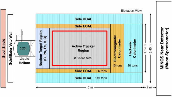
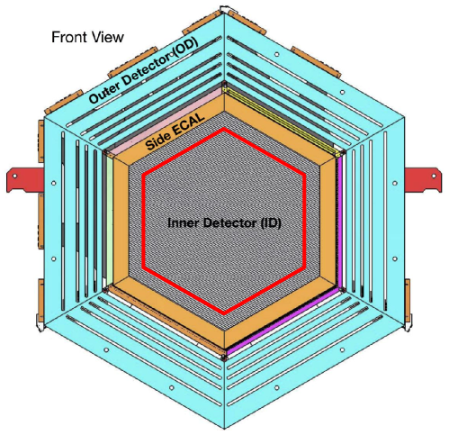
Figure 8: The MINERvA detector. The fiducial volume is illustrated by the red rectangle and hexagon (approximate scale)

The MINERvA detector records the energy and time of energy deposits (hits) in each scintillator strip. Hits are first grouped chronologically and then clusters of energy are formed by spatially grouping the hits in each scintillator plane. Clusters with energy $>1\,\mathrm{MeV}$ are then matched among the three views to create a track. The $\mu^{\pm}$ candidate is a track that exits the back of MINERvA matching a track of the expected charge entering the front of MINOS. The most upstream cluster on the muon track in MINERvA is taken to be the interaction vertex. The transverse position resolution of each track cluster is 2.7 mm and the angular resolution of the muon track is better than 10 mrad in each view. The reconstruction of the muon in the MINOS spectrometer gives a typical muon momentum of $11\%$. Charged $\pi^{\pm}$ reconstruction requires a second track originating from the vertex.

The MINERvA detector’s response is simulated by a tuned Geant4-based program. The energy scale of the detector is set by ensuring that both the photostatistics and the reconstructed energy deposited by momentum-analyzed through-going muons agree in data and simulation. The calorimetric constants used to reconstruct the energy of $\pi^{\pm}$ showers and the corrections for passive material are determined from the simulation bib:minerva_nim and verified by a test beam measurement bib:minerva_Tbeam .

VI Signal, Backgrounds and Data

VI.A Experimental Signature

In MINERvA, coherent scattering appears as two forward tracks originating from a common vertex with no additional visible energy near the vertex (Fig. 9). One, a muon, typically exits the downstream end of MINERvA and enters MINOS, producing a minimum ionizing track in both detectors. The other, a pion, produces a minimumally ionizing track before stopping or interacting hadronically within MINERvA. Visible energy near the vertex in addition to that from the minimally ionizing muon and pion is indicative of nuclear breakup in an incoherent interaction. In addition, the MINERvA detector enables reconstruction of the squared four-momentum transfered to the nucleus, $|t|$.

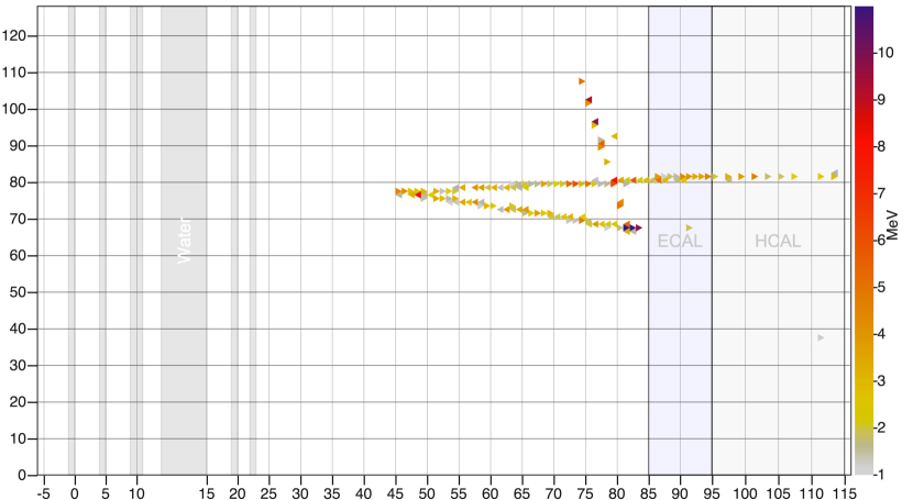
Figure 9: A data $\nu_{\mu}$ coherent scattering candidate. This visualization shows energy deposited in the vertical scintillator strips of the detector, with the numbering on the $x$-axis representing module number, the numbering on the $y$-axis representing strip number, and the color scale indicating the energy deposited in each strip.

VI.B Signal and Background Definitions

Signal interactions are simulated using the implementation of the Rein-Sehgal model bib:RS in GENIE bib:genie_manual Monte Carlo (MC), version 2.6.2, with the modifications described in Sec. VI.C.1. Events in the simulation are categorized as either signal or background as follows:

1. Signal (“Coherent”) - Interactions that produce a final state consisting of a muon, a charged pion, and the initial state nucleus. The only GENIE interactions that produce this final state are $\nu_{\mu}$ ($\overline{\nu}_{\mu}$) CC coherent pion production interactions. Coherent interactions on non-carbon nuclei are categorized as signal rather than background to avoid dependence of the background prediction on the signal model. The correction for non-carbon nuclei is described in Sec. X.D.

2. Charged-qurrent Quasielastic (“QE”) - $\nu_{\mu}$ ($\overline{\nu}_{\mu}$) CC quasielastic interactions as modeled in GENIE.

3. Non-Quasielastic, $W<1$ .4 GeV - $\nu_{\mu}$ ($\overline{\nu}_{\mu}$) CC interactions, excluding quasielastic, with true invariant mass $W<$ 1.4 GeV, where $W$ is the invariant mass of the hadronic recoil. This category is primarily delta resonance production, but also includes non-resonant pion production.

4. 1.4 $<W<$ 2.0 GeV - $\nu_{\mu}$ ($\overline{\nu}_{\mu}$) CC interactions with true invariant mass 1.4 $<W<$ 2.0 GeV. This is the transition region from delta resonance production to deep inelastic scattering.

5. $W>$ 2.0 GeV - $\nu_{\mu}$ ($\overline{\nu}_{\mu}$) CC interactions with true invariant mass $W>$ 2.0 GeV. This is the deep inelastic scattering (DIS) region.

6. Other - All other background interactions. This category is primarily wrong sign interactions (i.e. $\overline{\nu}_{\mu}$ instead of $\nu_{\mu}$ interactions and vice versa), but also includes non-$\nu_{\mu}$ ($\overline{\nu}_{\mu}$) and NC interactions. Wrong sign CC coherent pion production interactions are included in this category but are a small contribution.

VI.C Data and MC Samples

This analysis uses MINERvA data taken between November 2009 and April 2012 in the low energy $\nu_{\mu}$ and $\overline{\nu}_{\mu}$ beam configurations. The neutrino flux is normalized to the number of protons incident on the NuMI target (POT). The total POT for data taken in the $\nu_{\mu}$ ($\overline{\nu}_{\mu}$) beam configuration was $3.04\times 10^{20}$ ($2.00\times 10^{20}$). In $\overline{\nu}_{\mu}$ mode, $45\%$ of the POT were taken with a partial detector with 52$\%$ of the fiducial mass, meaning that $\sim$ 30% of the antineutrino coherent scattering events should occur in this partial detector.

The MC sample was generated with appropriate neutrino beam configurations, and was overlaid with data taken with the appropriate configuration to mimic pile-up effects in the data.

High-statistics signal-only MC samples were generated for estimating the resolution of the reconstructed kinematics, unfolding matrices, and selection efficiency for $\nu_{\mu}$ and $\overline{\nu}_{\mu}$ CC coherent scattering.

VI.C.1 Weighting Simulated Events

The MC was weighted to account for improvements in the understanding of (a) the neutrino flux, (b) the rate of neutrino interactions with single-pion final states, (c) the pion angle distribution in delta resonance decay, (d) the coherent pion production cross section in GENIE, and (e)MINOS muon tracking efficiency.

The MINERvA MC was generated with a flux prediction from a GEANT4 model of the NuMI target. The MC was subsequently weighted to reflect the flux prediction constrained by external hadron production data as described in Sec. V.

The GENIE prediction for single-pion final states was constrained by reanalyzed $\nu_{\mu}$-deuterium scattering data bib:D2Data . The axial vector mass for resonant pion production ($M^{RES}_{A}$) and corrections to the resonant pion production and nonresonant single pion production normalizations in GENIE were extracted from a fit of GENIE to the re-analyzed data for single-pion final states bib:D2Fit . Table 2 lists the values extracted from the fit. The default $M^{RES}_{A}$ in GENIE is 1.12 $\pm$ 0.22 GeV. Resonant interactions and nonresonant single pion production interactions in the MC were weighted to the values from the fit.

Parameter	Value
$M^{RES}_{A}$ (GeV)	0.94 $\pm$ 0.05
Resonant Normalization Correction	1.15 $\pm$ 0.07
Non-Resonant 1$\pi$ Normalization Correction	0.46 $\pm$ 0.04

Table 2: Parameters for single pion production in GENIE extracted from the fit of GENIE to re-analyzed $\nu_{\mu}$-deuterium scattering data from Ref. bib:D2Data .

GENIE assumes isotropic decay of baryon resonances from neutrino production, but the Rein-Seghal model predicts anisotropic baryon resonance decay. For $\Delta\to N\pi$ delta resonance decays, the angular distribution of the pion is given by

$$W_{\pi}(\cos\theta)=1-p_{\frac{3}{2}}P_{2}(\cos\theta)+p_{\frac{1}{2}}P_{2}(\cos\theta),$$ (11)

where $\theta$ is the pion angle in the $\Delta$ center of mass frame with respect to the $\Delta$ angular quantization axis, $p_{\frac{3}{2}}$ and $p_{\frac{1}{2}}$ are coefficients for the $m=\frac{3}{2}$ and $m=\frac{1}{2}$ states of the $\Delta$, respectively, and $P_{2}(\cos\theta)$ is the 2nd-order Legendre polynomial. For $\Delta\to N\pi$, GENIE simulates isotropic $\Delta$ decay with $p_{\frac{3}{2}}=p_{\frac{1}{2}}=0.5$, whereas the Rein-Sehgal resonance production model predicts non-isotropic $\Delta$ decay with $p_{\frac{3}{2}}=0.75$ and $p_{\frac{1}{2}}=0.25$. We weight the isotropic pion angle distribution from $\Delta^{++}\to N\pi$ decays as generated by GENIE to half the anisotropy predicted by the Rein-Seghal resonance production model, and consider both unweighted and fully-weighted anisotropies in setting systematic uncertainties.

We used the default INTRANUKE / hA model of final state interactions within the target nucleus (FSI) in GENIE.

The GENIE implementation of the Rein-Sehgal coherent scattering model uses measured total and inelastic cross sections for pion-proton and pion-deuterium scattering to calculate the pion-nucleus elastic scattering cross section. GENIE 2.6.2 contained an error in indexing the pion-proton and pion-deuterium cross section data tables. This error was corrected by weighting each MC signal event. The correction is less than $5\%$ in all $E_{\pi}$ bins in the analysis, except for $750<E_{\pi}<1000$ MeV, where the correction is $\sim 10\%$.

The efficiency of tracking the muon in MINOS differed between data and MC due to pile-up not being simulated in MINOS. The efficiency was measured in both data and MC by projecting muon tracks that exited MINERvA into MINOS and measuring the muon reconstruction rate in MINOS. The differences in efficiency between the data and MC were corrected for by weighting each MC event; the corrections were typically less than 5%.

VII Reconstruction

The muon is identified as the track that exits the downstream end of MINERvA and matches a track in MINOS. The reconstructed interaction vertex position is defined as the most upstream point along the MINERvA muon track. The pion track is the second track originating from the interaction vertex. Reconstruction produces, for each track, a 3D direction vector of its respective particle in each scintillator plane along the track. To reduce the effects of scattering, the direction of both the muon and pion are taken as the direction vector in the most upstream plane along their respective track. The angle between the directions of the muon (pion) and incoming neutrino is denoted by $\theta_{\mu}$ ($\theta_{\pi}$). The direction of the incoming neutrino is assumed to be parallel to neutrino beam axis.

The muon energy $E_{\mu}$ is reconstructed from the muon’s tracks in MINERvA and MINOS. The energy of the muon at its entrance point to MINOS is reconstructed from the MINOS track’s range (curvature in the magnetic field) if the muon stops inside (exits) MINOS. This energy is added to the calculated muon energy loss by ionization along the MINERvA track.

The pion energy $E_{\pi}$ is reconstructed by calorimetry under assumption that all hadronic (i.e. non-muon) visible energy results from interactions of the pion. To minimize sensitivity to mismodeled vertex activity for background events, hadronic visible energy within 200 mm of the interaction vertex is excluded from the $E_{\pi}$ reconstruction and replaced by a constant 60 MeV which is the average calorimetric energy deposited by a minimum ionizing pion over 200 mm in the tracker. Energy deposited in parts of the detector with passive layers (the side and downstream ECALs and HCALs) is corrected for the energy not observed in those passive layers. An overall calorimetric scale factor of $1.7$ is applied for $\pi^{\pm}$ response, as obtained from the simulation of signal events. Clusters of hits are included if they are between -20 ns and +30 ns of the reconstructed interaction vertex time. This requirement minimizes contamination from pile-up.

The reconstructed neutrino energy $E_{\nu}$ is $E_{\mu}+E_{\pi}$, where $E_{\mu}$ and $E_{\pi}$ are the reconstructed muon and pion energies, respectively. This calculation assumes zero energy transfer to the nucleus, which is a good approximation for coherent scattering since the nucleus remains in its ground state and the recoil of the nucleus is small due to small $|t|$.

The reconstructed square of the four-momentum transferred to the nucleus $|t|$ is calculated as

$$|t|=|(q-p_{\pi})^{2}|=|(p_{\nu}-p_{\mu}-p_{\pi})^{2}|,$$ (12)

where $p_{\nu}$, $p_{\mu}$, and $p_{\pi}$ are the reconstructed four-momentum vectors for the neutrino, muon, and pion, respectively. The reconstructed four-momentum vector for each particle is calculated from the particle’s reconstructed energy and direction. Likewise, the reconstructed squared four-momentum transferred from the lepton system $Q^{2}$ is calculated as

$$Q^{2}=-q^{2}=(p_{\nu}-p_{\mu})^{2}.$$ (13)

The resolution of the reconstructed interaction vertex position is $\sim$6 mm in the directions transverse to the beam and $\sim$12 mm parallel to the beam. Two-dimensional angular resolutions are $\sim$1 ^∘, although approximately 40% of the events where the $\pi^{\pm}$ scatters near the vertex have a significantly worse resolution, $\sim$10 ^∘. Muon energy resolution is $\sim$8 %, and $\pi^{\pm}$ energy resolution is $\sim$25 %. The resolution in $Q^{2}$ is $\sim$0.03 GeV², with about one in three events with worse resolution, up to $\sim$0.13 GeV². The resolution in $|t|$ is shown in Fig. 10.

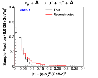
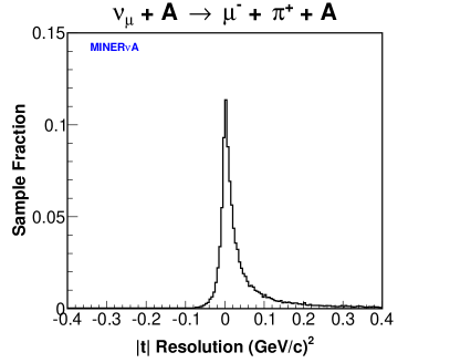
Figure 10: The reconstructed and true $|t|$ distributions (left) and the $|t|$ resolution, defined as $|t|_{\rm\textstyle reco}-|t|_{\rm\textstyle true}$, (right) for reconstructed $\nu_{\mu}$ CC coherent MC interactions inside the fiducial volume.

VIII Event Selection

This section describes the procedure for selecting candidate coherent scattering events from the data and MC for the measurement of the coherent scattering cross sections.

VIII.A Reconstruction and Fiducial Volume Cuts

Requiring exactly one reconstructed muon as described in Sec. VII gives a sample that is more than 99% pure $\nu_{\mu}$ or $\overline{\nu}_{\mu}$ CC events.

Each event is required to have exactly one additional track originating at the interaction vertex and pointing in the forward direction. For coherent events, this track identifies the pion and measures its direction.

The interaction vertex is required to be located within the fiducial volume. Dead time in the front end electronics bib:minerva_daq can result in an interaction upstream of the fiducial volume faking an interaction inside of it. This occurs when a portion of the visible energy deposited inside the fiducial volume by a muon from an upstream interaction is lost resulting in the muon track appearing to originate inside the fiducial volume. Many of these “dead time” events are also rejected by the requirement for a second track originating at the event vertex. Specifically, candidate events are rejected if strips on two or more planes intersected by the upstream track projection had dead time. Dead time is modeled in the MC by overlaying the MC with data and simulating the charge integration period for the channels in the MC containing charge from the data overlay.

VIII.B Muon Charge Cut

The muon charge is used to select either $\nu_{\mu}$ or $\overline{\nu}_{\mu}$ CC events. The muon charge is measured by the quantity $q/p$ extracted from the MINOS track fit, where $q$ and $p$ are the muon charge and momentum. Selected $\nu_{\mu}$ ($\overline{\nu}_{\mu}$) events have $q/p>0$ ($q/p<0$). Fig. 11 shows $q/p$ divided by the uncertainty on $q/p$ from the fit for events in the $\nu_{\mu}$ and $\overline{\nu}_{\mu}$ samples that pass the reconstruction and fiducial volume cuts of Sec. VIII.A. Prior to the $q/p$ cut, the $\overline{\nu}_{\mu}$ sample contains more wrong-sign ($\nu_{\mu}$) events than $\overline{\nu}_{\mu}$ events. This is because $\nu_{\mu}$ composes 15% of the flux in the $\overline{\nu}_{\mu}$ beam configuration and CC $\nu_{\mu}$ interactions produce a tracked hadron, either a proton or a pion, more often than CC $\overline{\nu}_{\mu}$ interactions.

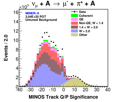
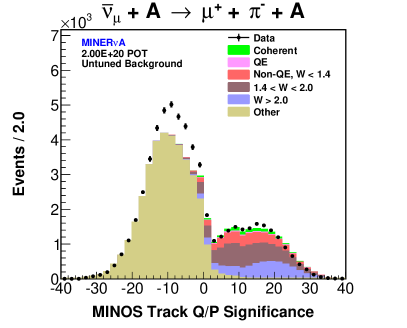
Figure 11: The $\nu_{\mu}$ (left) and $\overline{\nu}_{\mu}$ (right) $q/p$ divided by its uncertainty for the matched MINOS track for events that pass the reconstruction and fiducial volume cuts.

VIII.C Neutrino Energy Cut

The neutrino energy of the $\nu_{\mu}$ and $\overline{\nu}_{\mu}$ samples (Fig. 12) is restricted to $2.0<E_{\nu}<20\ \text{GeV}$. The $E_{\nu}$ $<$ 20 GeV requirement primarily excludes neutrinos resulting from kaon production at the NuMI target which are not well constrained. Note that muons that originate in the tracker and are tracked in MINOS have $E_{\mu}$ $>$ 1.5 GeV.

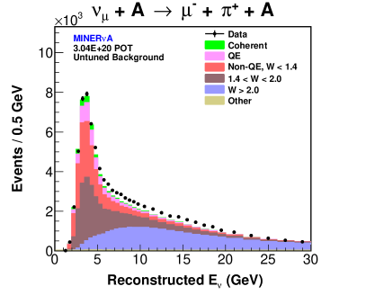
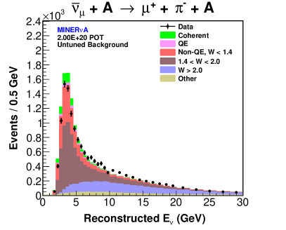
Figure 12: The $E_{\nu}$ distribution for events in the $\nu_{\mu}$ (left) and $\overline{\nu}_{\mu}$ (right) sample that pass all selection cuts up through the matched MINOS track $q/p$ cut. Events with $2.0<E_{\nu}<20\ \text{GeV}$ are selected.

VIII.D Proton Identification (Score) Cut

The visible energy along the hadron track is analyzed to reject events with a final state proton. The likelihood that the hadron track corresponds to a proton, referred to as the proton score, is calculated by comparing the visible energy in the clusters along the hadron track to the predicted energy deposition of a stopping proton and pion. The predicted energy deposition in each cluster is the product of the average $dE/dx$ in the scintillator, calculated by the Bethe-Bloch equation, and the path length of the track in the scintillator. In calculating $dE/dx$, the pion/proton momentum at each cluster is estimated by range along the hadron track. The reduced $\chi^{2}$ for comparing the visible energy to the predicted pion/proton energy deposition in the clusters along the hadron track is

$$\chi^{2}=\frac{1}{n}\displaystyle\sum_{i=1}^{n}\frac{\Delta E^{meas}_{i}-\Delta E^{pred}_{i}}{\sigma^{comb}_{i}},$$ (14)

where $\Delta E^{meas}_{i}$ is the measured deposited energy (i.e. visible energy), $\Delta E^{pred}_{i}$ is the predicted energy deposition, and $\sigma^{comb}_{i}$ is the combined uncertainty on $\Delta E^{meas}_{i}$ and $\Delta E^{pred}_{i}$ in the $i^{th}$ cluster along the hadron track with $n$ total clusters. The combined uncertainty $\sigma^{comb}_{i}$ consists of range fluctuations on the calculated $dE/dx$, photo-statistical uncertainty on the measured and predicted deposited energy, and uncertainty on the path length of the track in the scintillator bib:walton_thesis . The proton score is calculated as

$$\text{Proton Score}=1.0-\frac{\chi^{2}_{p}}{\sqrt{(\chi^{2}_{p})^{2}+(\chi^{2}_{\pi})^{2}}},$$ (15)

where $\chi^{2}_{p}$ and $\chi^{2}_{\pi}$ are the reduced $\chi^{2}$ for the predicted proton and pion energy deposition, respectively.

A particle that interacts in the detector may have one or more secondary tracks that emerge from its endpoint, representing either the scattered incident particle or particles produced in the interaction. For tracks with exactly one secondary track, the proton score is calculated from the secondary track, because proton/pion discrimination is at the Bragg peak. Events where the proton score was not calculated are selected. This occurs when there is more than one secondary track, or when the track exits the tracker. In the latter case, the proton score is unreliable because of the absorber layers in the calorimeters of the outer detector.

Figure 13 shows the proton score distribution for events in the $\nu_{\mu}$ and $\overline{\nu}_{\mu}$ samples. The category “Other Particles” consists primarily of charged kaons and neutrons that interacted near the event vertex. The disagreement between the data and MC in the proton score distribution is attributed to the MC prediction of neutrino pion production, which is subsequently tuned to data (see Sec. IX). The peak at 0.3 is due to clusters along the hadron track containing energy deposition from multiple particles. Events in the $\nu_{\mu}$ sample with proton score $<$ 0.4 are selected. Most events in the $\overline{\nu}_{\mu}$ sample with a tracked proton are rejected by the vertex energy cut, (see Sec. VIII.E) since these events tend to have additional final state charged hadrons due to charge conservation. A proton score cut is not imposed on the $\overline{\nu}_{\mu}$ sample to maximize the signal selection efficiency; in this sample, the quasielastic process is not a background.

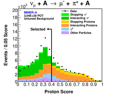
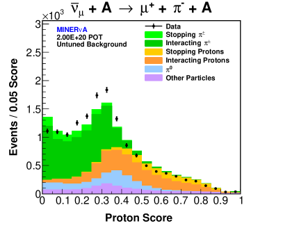
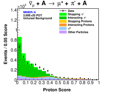
Figure 13: The top left (right) plot shows the proton score distribution for events, broken down by the true identity of the candidate hadron track, in the $\nu_{\mu}$ ($\overline{\nu}_{\mu}$) sample before applying cuts on proton score, on the vertex energy and on $|t|$. The bottom plot shows the same $\overline{\nu}_{\mu}$ sample, but after the vertex energy cut. The vertex energy cut rejects most events in the $\overline{\nu}_{\mu}$ sample with a tracked proton.

VIII.E Vertex Energy Cut

Coherent scattering produces a muon and charged pion in the forward direction while leaving the nucleus intact. Energy near the interaction vertex of each event is required to be consistent with the energy deposited by only a minimum ionizing muon and pion. Vertex energy $E_{vtx}$ is defined as the sum of the energies of clusters on the two vertex tracks within $\pm$5 planes ($\sim$110 mm in the longitudinal direction) from the event vertex, and clusters not on the two vertex tracks within $\pm$5 planes and 200 mm in the transverse direction from the event vertex. In calculating $E_{vtx}$, the cluster energies are corrected for passive material and the on-track cluster energies are corrected for the angle between their respective track and the perpendicular to the scintillator planes. This correction to normal incidence minimizes the dependence of the $E_{vtx}$ cut on the muon and pion kinematics. The $\pm$200 mm range in the transverse direction extends to the edge of the scintillator plane from the edge of the 850 mm fiducial volume apothem. Figure 14 shows the $E_{vtx}$ distribution for events in the $\nu_{\mu}$ ($\overline{\nu}_{\mu}$) sample that pass all selection cuts up through the proton score ($E_{\nu}$) cut. Events with 30 $<$ $E_{vtx}$ $<$ 70 MeV are selected. Requiring $E_{vtx}$ $>$ 30 MeV rejects events with a tracked $\gamma$ from the decay of a final state $\pi^{0}$, where the energy deposited by the $\gamma$ via $\gamma\to e^{+}e^{-}$ is separated from the event vertex.

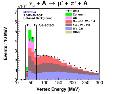
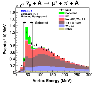
Figure 14: The left (right) plot shows the $E_{vtx}$ distribution for events in the $\nu_{\mu}$ ($\overline{\nu}_{\mu}$) sample that pass all selection cuts up through the proton score ($E_{\nu}$) cut. Events in the range 30 $<$ $E_{vtx}$ $<$ 70 MeV are selected.

VIII.F $|t|$ Cut

The final cut in the event selection is on $|t|$, which is necessarily small for coherent scattering; large $|t|$ is indicative of nuclear break-up in incoherent interactions. $|t|$ is calculated from the reconstructed four-momenta of the neutrino, muon and pion. The $\nu_{\mu}$ and $\overline{\nu}_{\mu}$ $|t|$ distributions with the tuned background prediction are shown in Fig. 15 for events passing all cuts up through the $E_{vtx}$ cut. Events with $|t|$ $<$ 0.125 $(\text{GeV/c})^{2}$ are selected.

A cut on $|t|$ could introduce a model dependence into the measured cross sections because of the $|t|$ dependence of the coherent cross section model in the MC. In both the Rein-Sehgal and Berger-Sehgal models, the $|t|$ dependence arises from the pion-nucleus elastic scattering cross section, which falls as $\exp(-b|t|)$ where $b$ is a free parameter. GENIE calculates the coherent scattering cross section on carbon using the Rein-Sehgal coherent model with $b\sim 40$ (GeV/c)^-2. In GENIE, 99% of the coherent events on carbon have true $|t|$ $<$ 0.125 $(\text{GeV/c})^{2}$. The pion-carbon elastic scattering cross section in the Berger-Sehgal model was fit to pion-carbon elastic scattering data for incident pion kinetic energies $\lesssim 1$ GeV, giving $b\gtrsim 60$ (GeV/c)^-2 bib:berger_sehgal . In addition, an exponential slope $b\sim 60$ (GeV/c)^-2 was measured from data of $\pi^{+}$ and $\pi^{-}$ elastic scattering on carbon at $\sim 2$ GeV/c incident pion momentum bib:pion_carbon_slope . The pion-carbon elastic scattering data suggest the cross section for coherent scattering on carbon in the MC should fall faster in $|t|$, which would result in $>$99% of MC coherent events on carbon having true $|t|$ $<$ 0.125 $(\text{GeV/c})^{2}$. To select low $|t|$ events, this analysis requires $|t|$ $<$ 0.125 $(\text{GeV/c})^{2}$. The high value of the $|t|$ cut makes its efficiency independent of variations in the $|t|$ distribution in different models.

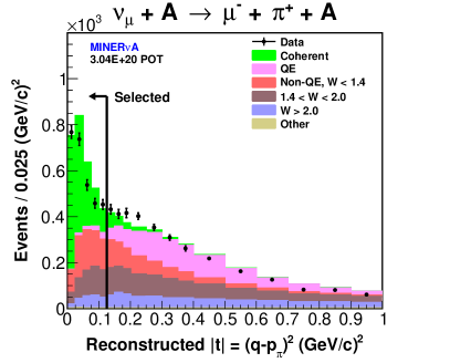
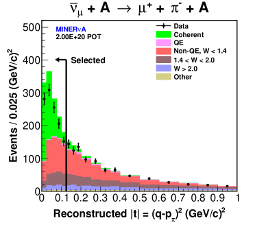
Figure 15: The $\nu_{\mu}$ (left) and $\overline{\nu}_{\mu}$ (right) $|t|$ distributions, after background tuning, for events passing all cuts up through the $E_{vtx}$ cut. Events with $|t|$ $<$ 0.125 $(\text{GeV/c})^{2}$ are selected.

IX Background Tuning

IX.A Sideband Scale Factors

The $\nu_{\mu}$ and $\overline{\nu}_{\mu}$ coherent candidate samples contain significant backgrounds. Uncertainties from the MC estimate are minimized by tuning the estimated background rates to data in a sideband. The sideband is defined as events with 0.2 $<$ $|t|$ $<$ 0.6 $(\text{GeV/c})^{2}$ that pass all selection cuts up through the vertex energy cut (Fig. 16). The requirement that events in the sideband pass the vertex energy cut minimizes sensitivity of the background tuning to mismodeled vertex activity (Sec. XII.C). This mismodeling could result in disagreement between data and the MC in the background acceptance of the vertex energy cut, and performing the background tuning after imposing the vertex energy cut will correct this disagreement.

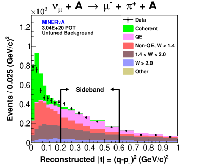
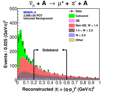
Figure 16: The $\nu_{\mu}$ (left) and $\overline{\nu}_{\mu}$ (right) $|t|$ distributions, before background tuning, for events that pass all selection cuts up through the vertex energy and proton score cuts. The sideband used for the background tuning are events with 0.2 $<$ $|t|$ $<$ 0.6 $(\text{GeV/c})^{2}$.

The background tuning extracts a correction to the normalization of each background. These background scale factors are determined by varying the normalizations of the backgrounds in a fit of the total MC to data in the sideband. The $\nu_{\mu}$ sideband $E_{\pi}$ distribution (Fig. 17) provides separation of the resonance, transition, and DIS processes, while the $\nu_{\mu}$ sideband $Q^{2}$ distribution (Fig. 17) separates resonance and QE processes. The $\nu_{\mu}$ background tuning therefore is performed with a fit to bins of $Q^{2}$ and $E_{\pi}$. Coherent scattering is a small contribution to the $\nu_{\mu}$ sideband and its scale factor is fixed to 1.0 in the fit. Other backgrounds are also a small contribution to the $\nu_{\mu}$ sample and their scale factor is also fixed to 1.0. The $\nu_{\mu}$ background scale factors extracted from the fit are listed in Table 3. The $\nu_{\mu}$ sideband $E_{\pi}$ and $Q^{2}$ distributions after applying the background scale factors to the MC are shown in Fig. 17.

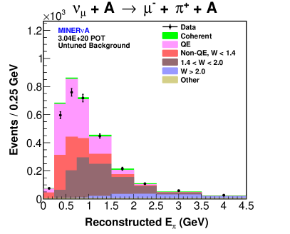
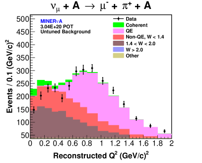
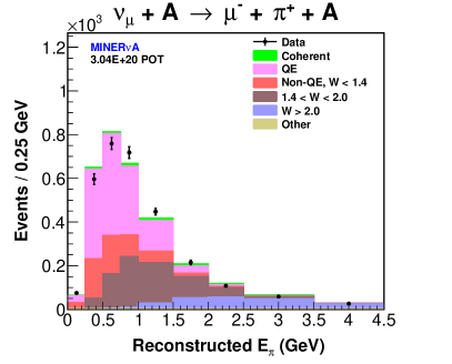
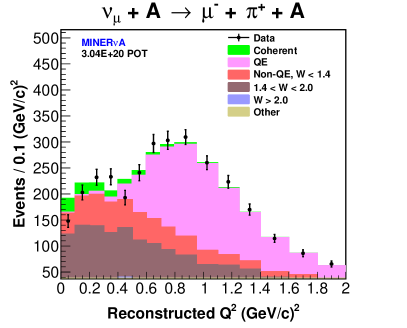
Figure 17: The $\nu_{\mu}$ sideband $E_{\pi}$ (left) and $Q^{2}$ (right) distributions before (top) and after (bottom) background tuning

The $\overline{\nu}_{\mu}$ background tuning is performed with a fit to the $\overline{\nu}_{\mu}$ sideband $E_{\pi}$ distribution (Fig. 18) only. Unlike the $\nu_{\mu}$ sample, QE is a small contribution to the $\overline{\nu}_{\mu}$ sample since the recoil neutron rarely produces a reconstructed track. This scale factor is fixed at 1.0. The $\overline{\nu}_{\mu}$ background scale factors extracted from the fit are listed in Table 3. The $\overline{\nu}_{\mu}$ sideband $E_{\pi}$ distribution after applying the background scale factors to the MC is shown in Fig. 18.

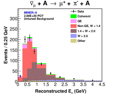
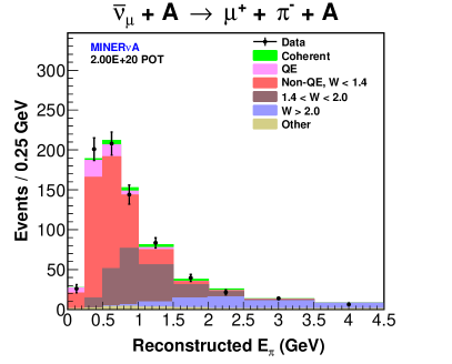
Figure 18: The $\overline{\nu}_{\mu}$ sideband $E_{\pi}$ distribution before (left) and after (right) background tuning

Background	$\nu_{\mu}$ Sample	$\overline{\nu}_{\mu}$ Sample
Charged-current quasielastic	1.13$\pm$0.04	1.0 (fixed)
Non-Quasielastic, $W_{gen}$ $<$ 1.4 GeV	0.73$\pm$0.08	1.07$\pm$0.08
1.4 $<$ $W_{gen}$ $<$ 2.0 GeV	0.81$\pm$0.05	0.79$\pm$0.09
$W_{gen}$ $>$ 2.0 GeV	1.7$\pm$0.2	2.3$\pm$0.3
Other	1.0 (fixed)	1.0 (fixed)

Table 3: Background scale factors

Background tuning corrects the normalization and provides evidence that the $E_{\pi}$ and $Q^{2}$ distributions of the backgrounds are likely correct. It does not correct all possible sources of uncertainty in the kinematics for each background. Mismodeling of the kinematics of the backgrounds is a source of systematic uncertainty as described later.

IX.B Pion Angle Weighting

Disagreement between data and MC remains in the $\nu_{\mu}$ and $\overline{\nu}_{\mu}$ sideband $\theta_{\pi}$ distributions after background tuning (Fig. 19). There is no model for the origin of this disagreement, and correct for it using data-driven weights of the total tuned background as a function of reconstructed $\theta_{\pi}$ (Fig. 19). For each group of two or more consecutive bins in the sideband $\theta_{\pi}$ distribution with tuned MC above (below) the data at greater than 1$\sigma$ statistical significance in each bin, the weighting decreases (increases) the total background in this group of bins by an amount required to bring the group’s agreement between data and MC to within 1$\sigma$. The $\nu_{\mu}$ and $\overline{\nu}_{\mu}$ sideband $\theta_{\pi}$ distributions after background tuning and $\theta_{\pi}$ weighting are shown in Fig. 19. The $\theta_{\pi}$ weighting is applied to the tuned background in the coherent-like sample. The change in the background prediction from the $\theta_{\pi}$ weighting is applied as a systematic uncertainty.

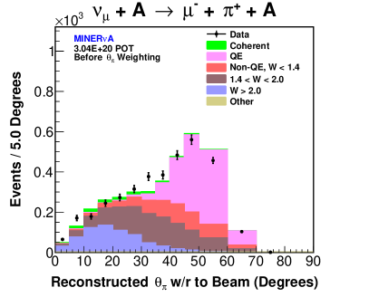
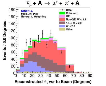
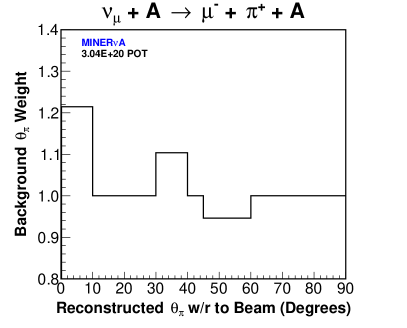
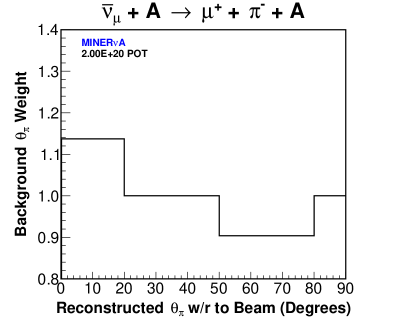
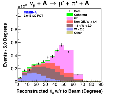
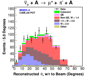
Figure 19: The top plots show the $\nu_{\mu}$ (left) and $\overline{\nu}_{\mu}$ (right) sideband $\theta_{\pi}$ distributions after background tuning. The middle plots show the $\theta_{\pi}$ weighting applied to the MC background to correct the disagreement between the data and the MC. The bottom plots show the sideband $\theta_{\pi}$ distributions after background tuning and $\theta_{\pi}$ weighting.

X Calculation of the Cross Sections

The measured cross section in true-$E_{\nu}$ bin $i$ is calculated as

$$\sigma_{i}=\frac{\beta\sum_{j}U_{ij}(N^{data}_{j}-N^{bkgd}_{j})}{T\phi_{i}\epsilon_{i}},$$ (16)

where $N^{data}_{j}$ is the number of data coherent candidates in reconstructed $E_{\nu}$ bin $j$, $N^{bkgd}_{j}$ is the tuned estimate of the number of background coherent candidates, $U_{ij}$ is the unfolding matrix element that estimates the signal contribution from reconstructed bin $j$ to true bin $i$, $\epsilon_{i}$ is the coherent selection efficiency, $\phi_{i}$ is the $\nu_{\mu}$ or $\overline{\nu}_{\mu}$ flux, $T$ is the number of carbon nuclei targets in the fiducial volume, and $\beta$ is the correction to the coherent event rate for interactions on non-carbon nuclei (see Sec. X.D). Differential cross sections as functions of $E_{\pi}$, $\theta_{\pi}$, and $Q^{2}$ are calculated similarly, but the flux is integrated over 2 $<E_{\nu}<$ 20 GeV.

The unfolding matrices and efficiency corrections for measuring the cross sections were estimated using coherent events in the MC, where events with $E_{\pi}$ $<$ 0.5 GeV were weighted by 50%. This weighting is referred to as the signal model weighting, and is discussed in Sec. X.E. The following sections detail each step of the cross section calculation.

X.A Unfolding

After background subtraction, the $\nu_{\mu}$ ($\overline{\nu}_{\mu}$) sample contains 1411 (481) coherent candidates. The distributions of the kinematic variables of these candidates are unfolded to correct for distortions and resolution effects created in the reconstruction process. The distributions were unfolded using the iterative unfolding method of D’Agostini bib:dagostini . The unfolding matrix $U_{ij}$ estimates the contribution from true bin $i$ to reconstructed bin $j$. It was calculated from the signal-only MC samples as

$$U_{ij}=\frac{N^{sel}_{ij}}{\sum_{j}N^{sel}_{ij}},$$ (17)

where $N^{sel}_{ij}$ is the number of coherent events passing all selection cuts in bin $ij$. The signal model weighting (Sec. X.E) was applied in calculating the unfolding matrices. In each successive iteration the unfolded distribution is recalculated in the same way from the unfolded distribution resulting from the previous iteration. The unfolding matrices for the $\nu_{\mu}$ are shown in Fig. 20, and $\overline{\nu}_{\mu}$ distributions are similar.

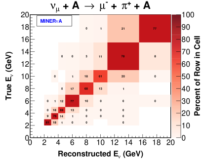
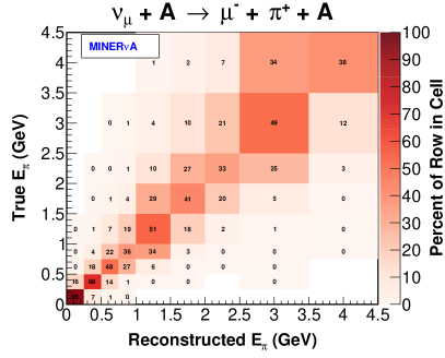
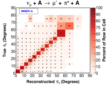
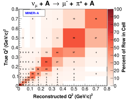
Figure 20: The unfolding matrices in $E_{\nu}$, $E_{\pi}$, $\theta_{\pi}$ and $Q^{2}$ for the $\nu_{\mu}$ sample.

The diagonal entries of the statistical covariance matrix increase with each unfolding iteration. The number of unfolding iterations, two, was optimized to give adequate correction of reconstruction distortion while minimizing the increase of these diagonals.

Unfolding creates correlations in the statistical uncertainty between bins which are included in the statistical covariance matrix.

X.B Efficiency Correction

After unfolding, the kinematic distributions are corrected for signal selection efficiency, which was estimated using coherent events from the signal MC samples. The efficiency in each true kinematic bin $\epsilon_{i}$ was calculated as

$$\epsilon_{i}=\frac{N^{sel}_{i}}{N^{gen}_{i}},$$ (18)

where $N^{gen}_{i}$ is the number of signal events generated inside the fiducial volume with true $E_{\nu}$ satisfying $2.0<E_{\nu}<20\ \text{GeV}$ in bin $i$, and $N^{sel}_{i}$ is the subset of those events that passed all reconstruction and selection cuts. The signal event weighting described earlier was applied in calculating the efficiency. The efficiency as a function of each kinematic parameter for the $\nu_{\mu}$ samples is shown in Fig. 21; the $\overline{\nu}_{\mu}$ efficiencies are similar. The overall efficiency for the $\nu_{\mu}$ and $\overline{\nu}_{\mu}$ samples is 24-25%.

The selection efficiency includes the acceptance of the reconstruction. The requirement that the muon be reconstructed in both MINERvA and MINOS limits $\theta_{\mu}$ of accepted events to $\theta_{\mu}$ $<$ $20^{\circ}$, and the minimum number of planes required to form a track limits $\theta_{\pi}$ of accepted events to $\theta_{\pi}$ $<$ $70^{\circ}$. For signal events in the MC occurring inside the fiducial volume, 96% have $\theta_{\mu}$ $<$ $20^{\circ}$ and $\theta_{\pi}$ $<$ $70^{\circ}$. About one third of the signal events are lost because the muon must have high enough energy to be tracked in the MINOS detector and then matched to a track in the MINERvA detector, and around half of the remaining signal events are lost by requiring the pion to make a second track in the event. Pion tracking drops off below $\sim$200 MeV and, as mentioned earlier, muon tracking fails below 1.5 MeV.

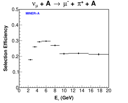
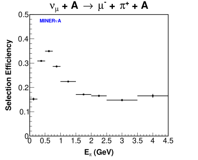
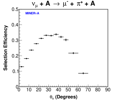
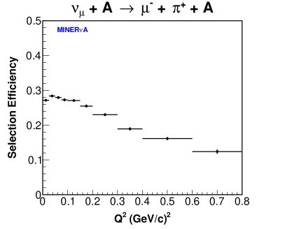
Figure 21: The selection efficiency as a function of $E_{\nu}$, $E_{\pi}$, $\theta_{\pi}$ and $Q^{2}$ for the $\nu_{\mu}$ sample.

X.C Flux Normalization

The cross sections were normalized to the flux prediction (see Sec. V) scaled to the POT for each sample. The cross section $\sigma_{i}$ in each $E_{\nu}$ bin $i$ was normalized to the flux integrated over the bin range (Table 15). The differential cross section $\left(\frac{d\sigma}{d\xi}\right)_{i}$ in each $\xi$ bin $i$ was normalized to the flux integrated over $2.0<E_{\nu}<20\ \text{GeV}$.

X.D Target Number Normalization

Nucleus	$A$	$T$ (units of 1029 nuclei)
1H	1.008	2.425
12C	12.011	2.404
16O	15.999	0.0655
27Al	26.982	0.0032
28Si	28.085	0.0032
35Cl	35.453	0.0051
48Ti	47.867	0.0047

Table 4: The nuclear mass number $A$ and estimated number of nuclei $T$ for each non-hydrogen nuclear species in the full detector fiducial volume, which spans the central 108 scintillator planes of the tracker and extends to the edges of a hexagon with an 850 mm apothem in the transverse (XY) plane.

The measured cross sections were normalized to the number of carbon nuclei (the “targets” of the neutrinos and antineutrinos) contained in the fiducial volume. The number of carbon nuclei was estimated using the detector geometry and material models, the latter of which was informed by direct material assay. The full (partial) detector fiducial volume contains 2.404 $\times$ 10²⁹ (1.246 $\times$ 10²⁹) carbon nuclei.

Non-carbon coherent interactions were not included in $N^{bkgd}$ to avoid dependence of the background estimate on the coherent model. Instead, the number of coherent candidates ($N^{coh}$) was corrected to the number of coherent candidates on carbon only ($N^{coh}_{c}$). The correction $\beta$ was calculated as

$$\beta=\frac{N^{coh}_{c}}{N^{coh}}=\frac{\phi\epsilon_{c}\sigma_{c}T_{c}}{\sum_{i}\phi\epsilon_{i}\sigma_{i}T_{i}},$$ (19)

where $\phi$ is the flux and $\epsilon_{i}$, $\sigma_{i}$, and $T_{i}$ are the coherent acceptance and selection efficiency, coherent cross section, and number of nuclei in the fiducial volume for nuclear species $i$. Assuming that the signal acceptance and selection efficiency is the same for all nuclear species and that the coherent cross section scales with the nuclear mass number $A$ as $A^{1/3}$ bib:RS ,

$$\beta\approx\frac{A^{1/3}_{c}T_{c}}{\sum_{i}A^{1/3}_{i}T_{i}}.$$ (20)

The estimated number of nuclei for each nuclear species in the full detector fiducial volume (Table 4) gives $\beta$ =  0.962. Diffractive scattering (see Sec. XI) is considered as a background rather than as a signal contribution.

X.E Signal Model Weighting

Initial measurements of the cross sections (Figs. 22–25) were made using unfolding matrices and efficiency corrections estimated from the unmodified GENIE Rein-Sehgal coherent model. These initial measurements revealed that GENIE over-predicts the production rate at low-$E_{\pi}$ and high-$\theta_{\pi}$. Better agreement between the GENIE prediction and the initial measurements was achieved by weighting the rate of interactions predicted by GENIE with $E_{\pi}$ $<$ 0.5 GeV by 50% (Fig.s 22–25). This is the signal model weighting. The $\chi^{2}$ for the comparison of the initial measurement of each cross section to the nominal and weighted GENIE predictions is listed in Table 5, where the $\chi^{2}$ was calculated per Eq. (26).

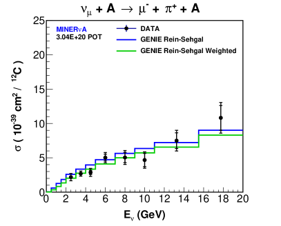
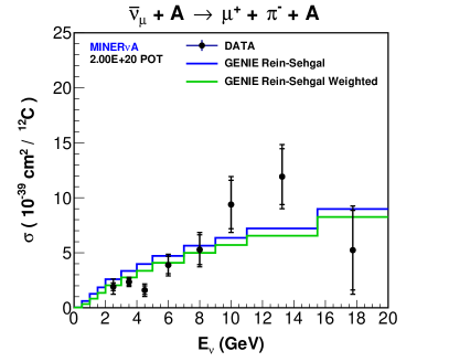
Figure 22: The initial measurements of the $\nu_{\mu}$ (left) and $\overline{\nu}_{\mu}$ (right) $\sigma(E_{\nu})$ made without the signal model weighting, and the GENIE prediction with and without the signal model weighting.

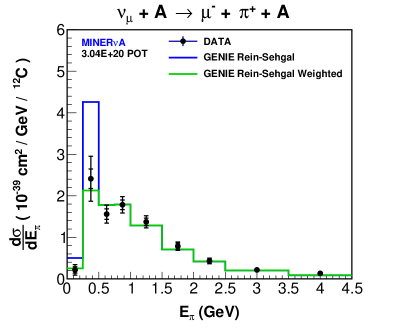
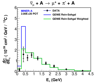
Figure 23: The initial measurements of the $\nu_{\mu}$ (left) and $\overline{\nu}_{\mu}$ (right) $\frac{d\sigma}{dE_{\pi}}$ made without the signal model weighting, and the GENIE prediction with and without the signal model weighting.

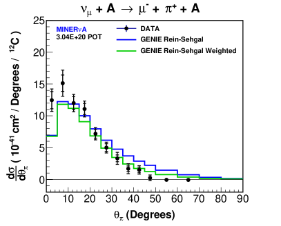
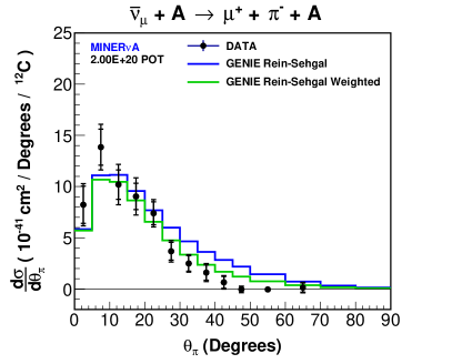
Figure 24: The initial measurements of the $\nu_{\mu}$ (left) and $\overline{\nu}_{\mu}$ (right) $\frac{d\sigma}{d\theta_{\pi}}$ made without the signal model weighting, and the GENIE prediction with and without the signal model weighting.

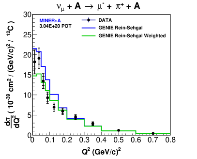
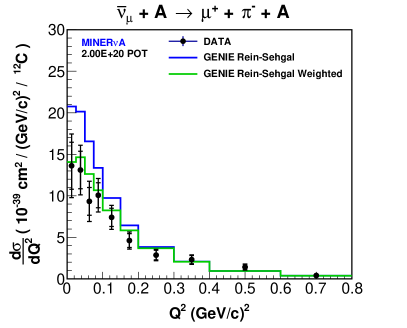
Figure 25: The initial measurements of the $\nu_{\mu}$ (left) and $\overline{\nu}_{\mu}$ (right) $\frac{d\sigma}{dQ^{2}}$ made without the signal model weighting, and the GENIE prediction with and without the signal model weighting.

Cross	$\nu_{\mu}\ \chi^{2}$		$\overline{\nu}_{\mu}\ \chi^{2}$
section	Nominal	Weighted	Nominal	Weighted	NDoF
$\sigma(E_{\nu})$	11.8	7.5	27.0	17.6	8
$d\sigma/dE_{\pi}$	22.4	13.5	16.6	7.1	9
$d\sigma/d\theta_{\pi}$	1388.4	418.8	144.1	46.9	12
$d\sigma/dQ^{2}$	19.2	15.4	16.8	10.0	10

Table 5: $\chi^{2}$ for the comparisons of the initial measured $\nu_{\mu}$ and $\overline{\nu}_{\mu}$ cross sections to the nominal and signal model weighted GENIE Rein-Sehgal predictions

To minimize bias on the measured cross sections from the signal model, the signal model weighting was applied to coherent events in the MC, the unfolding matrices and efficiency corrections were re-estimated, and the cross sections were remeasured. The effect of the signal model weighting on the measured cross sections is shown in Figs. 26–29. The signal model weighting did not actually change the selection efficiency as a function of $E_{\pi}$ since events in the numerator and denominator of the efficiency calculation (Eq. 18) in each $E_{\pi}$ bin were weighted equally. Instead, there was a change to the measured $\frac{d\sigma}{dE_{\pi}}$ resulting from the change to the $E_{\pi}$ unfolding matrix. The signal model weighting dramatically suppresses the peak in the 0.25-0.5 GeV bin in $E_{\pi}$ and thereby the predicted amount of migration from that bin, resulting in a decrease of the measured $\nu_{\mu}$ and $\overline{\nu}_{\mu}$ $\frac{d\sigma}{dE_{\pi}}$ in the 0.25-0.5 GeV bin and an increase in the adjacent bins.

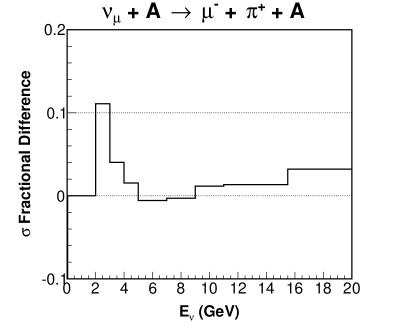
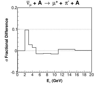
Figure 26: The effect of the signal model weighting on the measured $\nu_{\mu}$ (left) and $\overline{\nu}_{\mu}$ (right) $\sigma(E_{\nu})$.

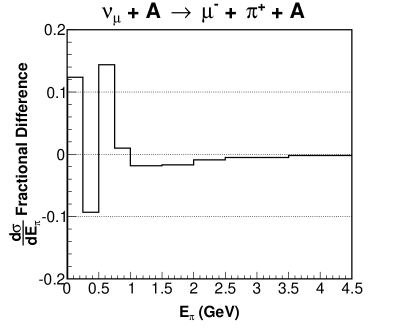
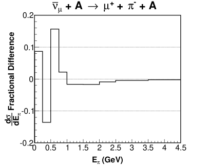
Figure 27: The effect of the signal model weighting on the measured $\nu_{\mu}$ (left) and $\overline{\nu}_{\mu}$ (right) $\frac{d\sigma}{dE_{\pi}}$.

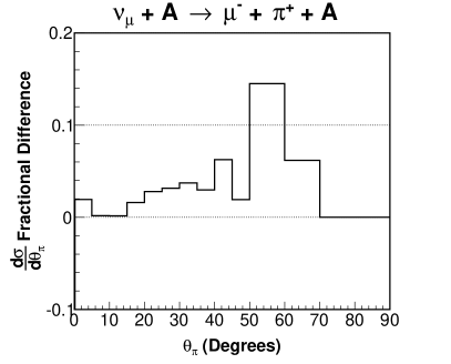
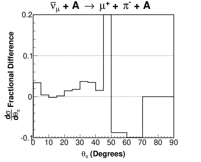
Figure 28: The effect of the signal model weighting on the measured $\nu_{\mu}$ (left) and $\overline{\nu}_{\mu}$ (right) $\frac{d\sigma}{d\theta_{\pi}}$.

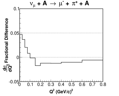
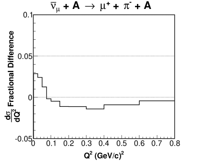
Figure 29: The effect of the signal model weighting on the measured $\nu_{\mu}$ (left) and $\overline{\nu}_{\mu}$ (right) $\frac{d\sigma}{dQ^{2}}$.

XI Contribution From Diffractive Scattering

Diffractive pion production from free protons may appear in the detector with the same signature as coherent pion production, if the recoiling proton is undetected. Although the recoil system is never detected for coherent scattering on heavier nuclei, diffractive scattering is not the same process and is considered a background. It was not included in the MC simulations of backgrounds, and can be constrained from the data. An exclusive calculation of the diffractive cross section valid in the kinematic region of the measured coherent cross sections does not yet exist. The PCAC-based calculation of diffractive scattering by Rein bib:rein_diffractive is valid only for $W>2$ GeV, since the interference with $p\pi$ final states from neutrino resonance production must be calculated for $W<2$ GeV. For diffractive scattering at small-$|t|$, $W>2$ GeV corresponds to $E_{\pi}$ $>$ 1.5 GeV, which covers only the high-$E_{\pi}$ phase space of the measured coherent cross sections. A search for diffractive scattering within the selected coherent candidate sample by looking for ionization from the recoil proton near the event vertex is presented here.

XI.A Diffractive Acceptance

Coherent and diffractive scattering in the detector only differ in acceptance because of the presence of the recoiling proton. The relative diffractive-to-coherent acceptance of the vertex energy cut is a function of $|t|$ since the kinetic energy of the proton, $T_{p}$, is proportional to $|t|$. This relative acceptance was estimated using a distribution of vertex energy deposited by recoil protons as a function of $T_{p}$, which was estimated from a simulation of single protons originating in the fiducial volume and isotropic in direction along with a coherent MC sample passing all selection cuts up to the vertex energy cut. For each event, the vertex energy from a recoil proton with kinetic energy $T_{p}$ was added to the vertex energy of the event. The relative diffractive-to-coherent acceptance (Fig. 30) was calculated as the ratio of the vertex energy cut acceptance with this added vertex energy to the acceptance without this added vertex energy, as a function of $|t|$, which was calculated event-by-event. The vertex energy cut acceptance is insensitive to differences between diffractive and coherent scattering in the muon and pion kinematics since the energy deposited by the muon and pion is corrected to normal incidence in the vertex energy calculation.

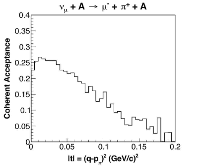
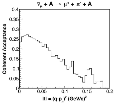
Figure 30: The $\nu_{\mu}$ (left) and $\overline{\nu}_{\mu}$ (right) estimated relative diffractive-to-coherent acceptance (top), coherent acceptance (middle), and absolute diffractive acceptance (bottom) as a function of $|t|$. The absolute diffractive acceptance was estimated by weighting the coherent acceptance by the relative diffractive-to-coherent acceptance.

The vertex energy cut rejects nearly all diffractive events with $|t|$ $>$ 0.125 $(\text{GeV/c})^{2}$. Since the signal sample has reconstructed $|t|$ $<$ 0.125 $(\text{GeV/c})^{2}$, both types of events have low $|t|$, and the acceptance of the $|t|$ cut is approximately the same for both of them after cutting on vertex energy. The acceptance as a function of true $|t|$ can therefore be estimated by weighting the relative diffractive-to-coherent acceptance of the vertex energy cut by the total selection efficiency for coherent scattering as a function of true $|t|$ (Fig. 30). Note though that the coherent acceptance is non-zero above $|t|$ = 0.125 $(\text{GeV/c})^{2}$ due to the reconstructed $|t|$ resolution.

The diffractive scattering contribution to the sideband (0.2 $<$ $|t|$ $<$ 0.6 $(\text{GeV/c})^{2}$) is negligible and diffractive scattering is neglected in tuning the GENIE prediction of the incoherent backgrounds.

XI.B Diffractive Cross Section Estimate

An estimate of the diffractive cross section can be made from a calculation of inclusive $\nu_{\mu}p\to\mu^{-}\pi^{+}p$ and $\overline{\nu}_{\mu}p\to\mu^{+}\pi^{-}p$ on free protons by Kopeliovich et al. bib:kopeliovich which uses Adler’s PCAC relation and pion-nucleus scattering data. Relative to the GENIE prediction, the Kopeliovich calculation exhibits a low-$|t|$ enhancement from all processes, including that from diffractive scattering, not present in GENIE. The low-$|t|$ enhancement as extracted from the Kopeliovich calculation is therefore an estimate of the largest possible diffractive cross section in this model.

The diffractive and non-diffractive components of the Kopeliovich calculation were estimated by fitting the GENIE prediction plus an exponential term to the Kopeliovich $\frac{d\sigma}{d(|t|-|t|_{min})}$ prediction (Fig. 31). The Kopeliovich cross section was fit as a function of $|t|-|t|_{min}$ since, for diffractive scattering, $\frac{d\sigma}{d|t|}$ will deviate from an exponential at low $|t|$ due to $|t|_{min}$ suppression, whereas $\frac{d\sigma}{d(|t|-|t|_{min})}$ will not. The fit range was 0 $<$ $|t|-|t|_{min}$ $<$ 0.25 $(\text{GeV/c})^{2}$, which covers the range of non-zero diffractive acceptance. The Kopeliovich $\frac{d\sigma}{d(|t|-|t|_{min})}$ was fit for $E_{\nu}$ = 4.0 GeV, which is near the average $E_{\nu}$ of the neutrino flux. Further details of the fit may be found in bib:Mislivec_thesis .

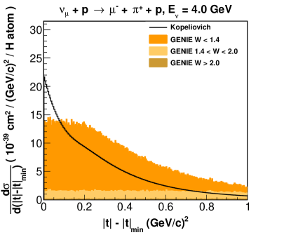
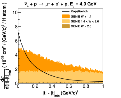
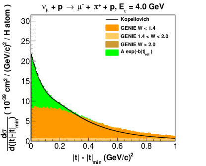
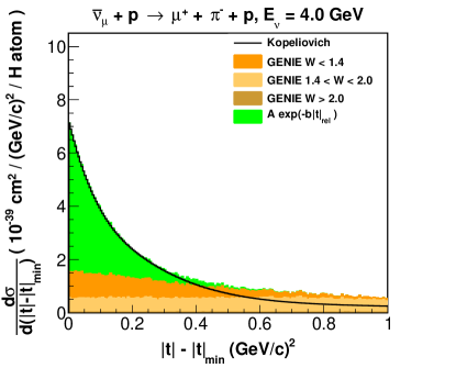
Figure 31: The $\nu_{\mu}$ (left) and $\overline{\nu}_{\mu}$ (right) Kopeliovich and GENIE predicted $\frac{d\sigma}{d(|t|-|t|_{min})}$ for $E_{\nu}$ = 4.0 GeV before (top) and after (bottom) fitting the Kopeliovich prediction. The fit includes an exponential term representing the diffractive $\frac{d\sigma}{d(|t|-|t|_{min})}$.

The diffractive $\frac{d\sigma}{d|t|}$ was estimated by subtracting the GENIE $\frac{d\sigma}{d|t|}$ from the Kopeliovich $\frac{d\sigma}{d|t|}$, where the GENIE $\frac{d\sigma}{d|t|}$ was scaled by the normalization scale factors extracted from the fit to the Kopeliovich $\frac{d\sigma}{d(|t|-|t|_{min})}$.

The $\nu_{\mu}$ and $\overline{\nu}_{\mu}$ diffractive cross sections at $E_{\nu}$ = 4 GeV (Table 6) were obtained by integrating the exponential extracted from the fit to the Kopeliovich $\frac{d\sigma}{d(|t|-|t|_{min})}$. The $\nu_{\mu}$ ($\overline{\nu}_{\mu}$) diffractive cross section is 34% (19%) of the GENIE coherent cross section on carbon at $E_{\nu}$ = 4 GeV. The acceptance-reduced diffractive cross sections were calculated by weighting the diffractive $\frac{d\sigma}{d|t|}$ by the relative diffractive-to-coherent acceptance of the vertex energy cut as a function of $|t|$ and integrating over $|t|$. The diffractive scattering contribution to the measured $\nu_{\mu}$ ($\overline{\nu}_{\mu}$) coherent cross sections is 8% (4%). Again, this is an estimate of the largest possible diffractive contribution.

	$\sigma$ ( 10-39 cm2 / atom )
	$\nu_{\mu}$	$\overline{\nu}_{\mu}$
Diffractive on H	1.24 (0.34)	0.69 (0.19)
Acceptance Reduced	0.28 (0.08)	0.15 (0.04)
Diffractive on H
GENIE Coherent on 12C	3.64	3.64

Table 6: The maximum estimated diffractive cross section, the same cross section with acceptance reduction, and the GENIE coherent cross section for comparison at $E_{\nu}$ = 4.0 GeV. The numbers in the parentheses are the fraction of the coherent cross section.

XI.C Search for Diffractive Scattering

The search for diffractive interactions within the selected coherent candidate samples looks for ionization from the recoil proton near the event vertex. Accepted diffractive interactions are estimated to have $|t|$ $\lesssim$ 0.1 $(\text{GeV/c})^{2}$, corresponding to a recoil proton with $T_{p}$ $\lesssim$ 50 MeV and range $\lesssim$ 2 cm in the scintillator. The search region for the recoil proton ionization extends $\pm$2 planes (34 mm of scintillator) in the longitudinal direction, and $\pm$2 strip widths (66 mm of scintillator) in the transverse direction, from the event vertex. For selected diffractive interactions, the recoil proton is identified by a large energy deposition in a single strip inside the search region.

Figure 32 shows the distribution of maximum vertex strip energy (MVSE), defined for each event as the largest amount of visible energy in a single strip inside the search region, for the $\nu_{\mu}$ and $\overline{\nu}_{\mu}$ selected coherent-like samples. The region of large MVSE where the MC coherent contribution is small is indicative of ionization in addition to that from a muon and pion only and is analyzed for the presence of diffractive interactions.

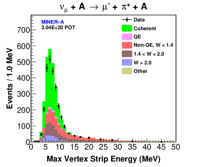
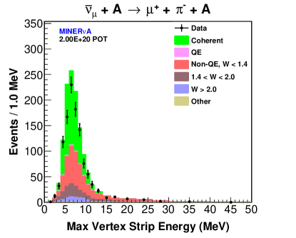
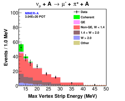
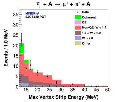
Figure 32: The MVSE for the $\nu_{\mu}$ (left) and $\overline{\nu}_{\mu}$ (right) selected coherent candidate samples. The bottom plots show the high-MVSE region examined for the presence of diffractive scattering. The non-diffractive background normalizations are tuned.

As mentioned previously, diffractive scattering was not simulated in the MC. Instead, a stand-in diffractive MC sample was constructed from MC interactions from other processes that pass all selection cuts and have a final state consisting of a muon, a charged pion, and a proton. This sample was then weighted (Fig. 33) as a function of $|t|$ (calculated from the proton kinetic energy) to the shape of the diffractive $\frac{d\sigma}{d|t|}$ weighted by the absolute diffractive acceptance (Fig. 30).

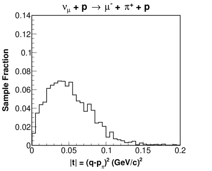
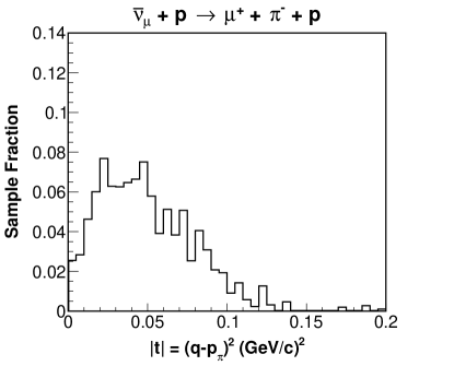
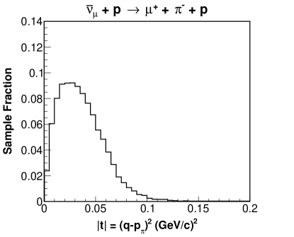
Figure 33: The $\nu_{\mu}$ (left) and $\overline{\nu}_{\mu}$ (right) diffractive MC $|t|$ distributions before (top) and after (bottom) weighting to the shape of the diffractive $\frac{d\sigma}{d|t|}$ weighted by the absolute diffractive acceptance.

The MVSE distribution was tested for the presence of diffractive scattering by adding the diffractive MC to the existing background tuned MC (Fig. 34) and fitting the diffractive normalization. The fit was performed in the region 16 $<$ MVSE $<$ 40 MeV where the coherent contribution is small. The $\chi^{2}$ in the fit was calculated as

$$\chi^{2}=AC^{-1}A^{T},$$ (21)

where $C$ is the total covariance (statistical + systematic) matrix for the MVSE distribution in the fit region, and

$$A_{i}=N_{i}^{data}-N_{i}^{MC}-N_{i}^{diff},$$ (22)

where $N_{i}^{data}$, $N_{i}^{MC}$, and $N_{i}^{diff}$ are the data, non-diffractive MC, and diffractive MC event rates, respectively, in MVSE bin $i$ within the fit region. The non-diffractive MC event rate was held constant in the fit.

The $\nu_{\mu}$ ($\overline{\nu}_{\mu}$) ratio of diffractive to coherent MC integrated event rates extracted from the fit is +0.01$\pm$0.08 (-0.03$\pm$0.09), which is consistent with the estimated 8% (4%) estimate of the largest possible diffractive contribution to the measured coherent cross sections. These results are also consistent with no diffractive scattering contribution to our measured coherent cross sections, and the measured coherent cross sections are not corrected for the possible contribution from diffractive scattering.

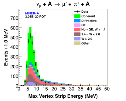
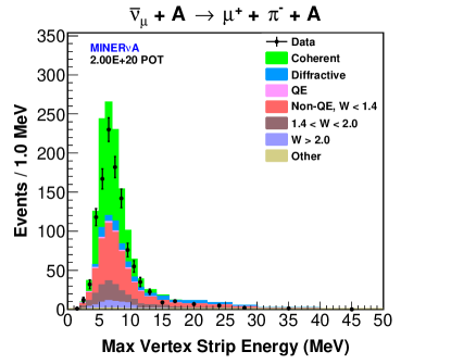
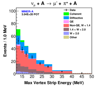
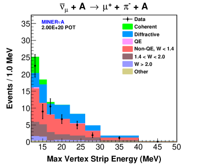
Figure 34: The MVSE distribution for the $\nu_{\mu}$ (left) and $\overline{\nu}_{\mu}$ (right) selected coherent-like samples. The bottom plots show the high-MVSE region examined for the presence of diffractive scattering. The non-diffractive background normalizations are tuned. The added diffractive MC sample shown is for 0.2 relative diffractive-to-coherent normalization, which is clearly inconsistent with the data. The fitted $\nu_{\mu}$ ($\overline{\nu}_{\mu}$) relative diffractive-to-coherent normalization is +0.01$\pm$0.08 (-0.03$\pm$0.09).

XII Systematic Uncertainties

The cross section measurements relied on the MC to estimate the background, resolution of the kinematic parameters, signal selection efficiency, and to some extent, the flux. Uncertainties on the predictions of the MC therefore result in uncertainties on the measured cross sections. These uncertainties and their correlations are evaluated by simulating an ensemble of pseudoexperiments with different assumptions about each systematic uncertainty with altered background and event migration in each pseudoexperiment. The results of those pseudoexperiments then determine a covariance matrix of systematic uncertainties.

The systematic uncertainties in the measured cross sections are shown in Figs. 35–38. The interaction model and detector model uncertainties in these figures are decomposed into their constituent uncertainties. The fractional systematic uncertainties tend to be larger for the $\overline{\nu}_{\mu}$ cross sections than the $\nu_{\mu}$ cross sections. This is due to the larger background fraction in the $\overline{\nu}_{\mu}$ candidate sample, coupled with the systematic uncertainties on the background prediction.

The evaluation of the systematic uncertainties on the measured cross sections is detailed in the following sections. The effects of the individual systematic uncertainties on each measured quantity can be found in Ref. bib:Mislivec_thesis .

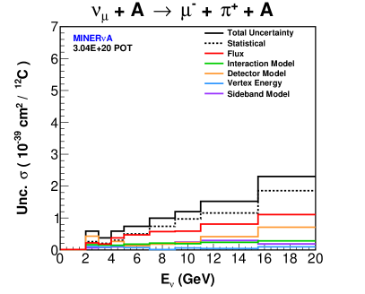
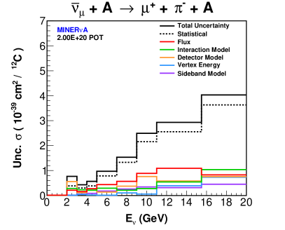
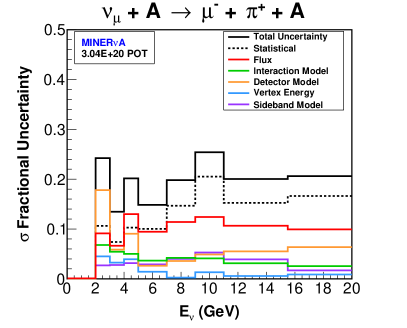
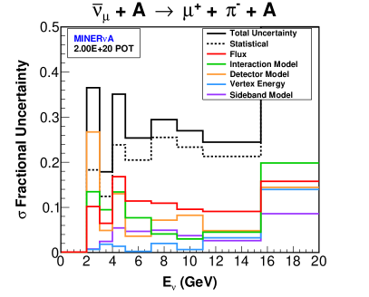
Figure 35: The statistical and systematic uncertainties on the measured $\sigma(E_{\nu})$ for $\nu_{\mu}$ (left) and $\overline{\nu}_{\mu}$ (right). The top (bottom) plots show the absolute (fractional) uncertainty.

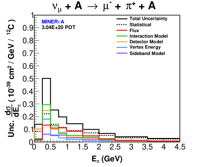
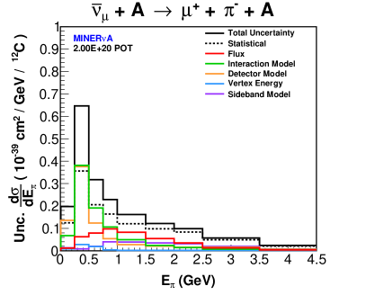
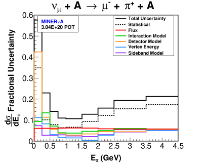
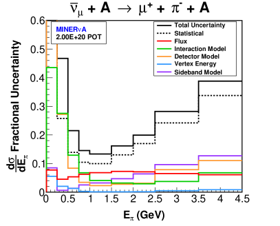
Figure 36: The statistical and systematic uncertainties on the measured $\frac{d\sigma}{dE_{\pi}}$ for $\nu_{\mu}$ (left) and $\overline{\nu}_{\mu}$ (right). The top (bottom) plots show the absolute (fractional) uncertainty. In the 0-0.25 GeV bin, the fractional uncertainty is large due to the small measured cross section.

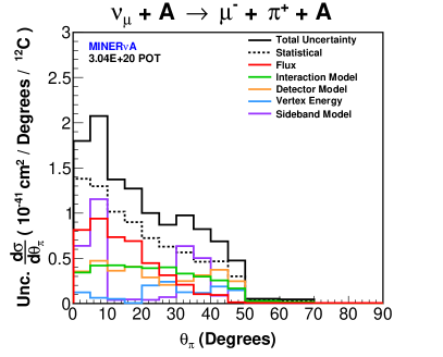
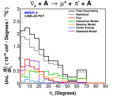
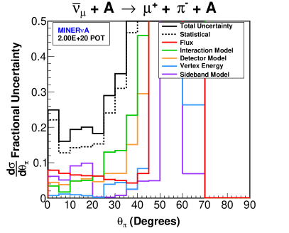
Figure 37: The statistical and systematic uncertainties on the measured $\frac{d\sigma}{d\theta_{\pi}}$ for $\nu_{\mu}$ (left) and $\overline{\nu}_{\mu}$ (right). The top (bottom) plots show the absolute (fractional) uncertainty. At high-$\theta_{\pi}$, the fractional uncertainty is large due to the small measured cross section.

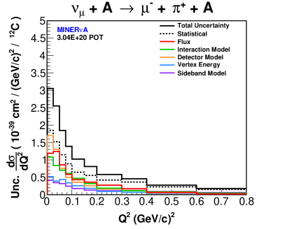
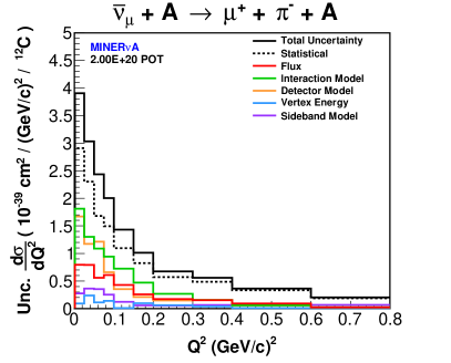
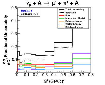
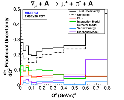
Figure 38: The statistical and systematic uncertainties on the measured $\frac{d\sigma}{dQ^{2}}$ for $\nu_{\mu}$ (left) and $\overline{\nu}_{\mu}$ (right). The top (bottom) plots show the absolute (fractional) uncertainty.

XII.A Flux

The uncertainty on the flux prediction, detailed in bib:flux , consists of uncertainties that govern hadronic interactions in the NuMI target and downstream beamline materials, uncertainties in the magnetic focusing of hadrons emerging from the target, and the geometry model of the beamline components. The flux uncertainty was evaluated from a set of 100 alternate flux predictions. Each alternate flux prediction, referred to herein as a flux variation, was the result of simultaneously varying the parameters in the flux model, where each parameter was varied by a random amount determined from a gaussian distribution centered on the nominal parameter value with a 1$\sigma$ width equal to the parameter uncertainty. To evaluate the flux uncertainty on the cross sections, the cross sections were remeasured for each flux variation and a covariance matrix for the set of flux variations was calculated for each cross section.

XII.B Neutrino Interaction Model

The cross section measurements rely on the MC to predict the rate of the incoherent backgrounds. The measured cross sections are therefore subject to uncertainties on the underlying neutrino-nucleus interaction models of GENIE. For the purpose of evaluating the effects of these uncertainties, GENIE provides event-by-event weights. These weights modify the predictions of the cross section models and FSI models. These weights modify both the normalization and kinematic dependence of the model predictions. The weights used to evaluate the neutrino-nucleus interaction model uncertainties on the measured cross sections correspond to $\pm 1\sigma$ uncertainties on the GENIE model parameters. Table 7 lists the default $\pm 1\sigma$ uncertainties on these parameters for the MINERvA implementation of GENIE used in this analysis.

Parameter	Variation
CC Quasielastic
Normalization	+20%, -15%
Axial vector mass (shape only)	$\pm$10%
Vector form factor model (shape only)	BBBA to
	dipole
	parameterization
Pauli suppression	$\pm$30%
NC Elastic
Axial vector mass	$\pm$25%
Strange axial form factor $\eta$	$\pm$30%
CC Resonance Production
Normalization	$\pm$20%
Axial vector mass	$\pm$20%
Vector mass	$\pm$10%
CC & NC Non-Resonant Pion Production
Normalization of 1$\pi$ final states from $\nu p$ / $\overline{\nu}p$	$\pm$50%
Normalization of 1$\pi$ final states from $\nu n$ / $\overline{\nu}n$	$\pm$50%
Normalization of 2$\pi$ final states from $\nu p$ / $\overline{\nu}p$	$\pm$50%
Normalization of 2$\pi$ final states from $\nu n$ / $\overline{\nu}n$	$\pm$50%
Deep Inelastic Scattering
Bodek-Yang model parameter $A_{HT}$	$\pm$25%
Bodek-Yang model parameter $B_{HT}$	$\pm$25%
Bodek-Yang model parameter $C_{V1u}$	$\pm$30%
Bodek-Yang model parameter $C_{V2u}$	$\pm$40%
Final State Interactions
Nucleon mean free path	$\pm$20%
Nucleon charge exchange probability	$\pm$50%
Nucleon elastic interaction probability	$\pm$30%
Nucleon inelastic interaction probability	$\pm$40%
Nucleon absorption probability	$\pm$20%
Nucleon $\pi$-production probability	$\pm$20%
$\pi$ mean free path	$\pm$20%
$\pi$ charge exchange probability	$\pm$50%
$\pi$ elastic interaction probability	$\pm$10%
$\pi$ inelastic interaction probability	$\pm$40%
$\pi$ absorption probability	$\pm$30%
$\pi$ $\pi$-production probability	$\pm$20%
Hadronization and Resonance Decay
$x_{F}$ dependence for $N\pi$ final states
in AGKY hadronization model	$\pm$20%
Resonance $\to X+1\gamma$ branching ratio	$\pm$50%
Pion angular distribution in $\Delta^{++}\to N\pi$	Isotropic $\to$
	Rein-Sehgal
	parameterization

Table 7: The default $\pm 1\sigma$ variations to the GENIE model parameters.

The GENIE prediction of single-pion final states was fit to $\nu_{\mu}$ deuterium scattering data bib:D2Data ; bib:D2Fit . This fit resulted in improved values and reduced uncertainties for the axial vector mass for resonant pion production $M^{RES}_{A}$, and the resonant pion production and non-resonant single pion production normalizations in GENIE. Furthermore, the uncertainty on the vector mass for resonant pion production $M^{RES}_{V}$ was reduced from the GENIE default $\pm$10% to $\pm$3%. This reduction was supported by comparisons of predicted and measured helicity amplitudes for resonance production in electron-nucleus scattering bib:mvres_constraint . The reduced CC resonance production and CC non-resonant single pion production uncertainties are listed in Table 8.

Parameter	Variation
CC Resonance Production
Normalization	$\pm$7%
Axial vector mass	$\pm$5%
Vector mass	$\pm$3%
CC & NC Non-Resonant Pion Production
Normalization of 1$\pi$ final states from $\nu p$ / $\overline{\nu}p$	$\pm$4%
Normalization of 1$\pi$ final states from $\nu n$ / $\overline{\nu}n$	$\pm$4%

Table 8: The reduced $\pm 1\sigma$ variations to the CC resonance production and CC non-resonant single pion production model parameters in GENIE.

As discussed in Sec. VI.C.1, the isotropic $\Delta^{++}\to N\pi$ decay in the MC was weighted to half the non-isotropy predicted by the Rein-Sehgal resonance production model. The uncertainty on the decay isotropy applied to the measured cross sections was half the difference between the isotropic and non-isotropic predictions. This is a reduction of the default GENIE uncertainty, which is the full difference between the isotropic and non-isotropic predictions.

The uncertainty on the measured cross sections does not include uncertainty intrinsic to the Rein-Sehgal model of coherent production in the MC. The MINERvA implementation of GENIE 2.6.2 did not include event weights for these uncertainties. In principle, the uncertainty in the measured cross sections should include uncertainty in the signal model due to the signal model dependence introduced by the unfolding and efficiency correction. Bias from the signal model was evaluated by remeasuring the cross sections with the signal model weighted to the initial cross section measurements; the differences in the extracted cross sections were small compared to the total uncertainty. We found that the remaining bias is small compared to the total uncertainty in the cross sections.

The largest GENIE uncertainties in the measured $\nu_{\mu}$ cross sections are the uncertainties in the pion inelastic interaction and pion absorption rates of the FSI model, and the uncertainty in the $\Delta^{++}$ decay isotropy. The largest GENIE uncertainties on the measured $\overline{\nu}_{\mu}$ cross sections are the uncertainties on the neutron elastic interaction and neutron absorption rates in the FSI model.

XII.C Vertex Energy

For non-coherent interactions in the MC, the amount of visible energy near the event vertex is dependent upon the modeling of initial and final state nuclear effects in GENIE. Since vertex energy is used to reject non-coherent interactions, the predicted rate of background is thereby sensitive to the modeling of these effects. This sensitivity was minimized by tuning the background prediction to data after cutting on vertex energy. Uncertainties on the measured cross sections from modeling final state interactions in the nucleus were evaluated using the GENIE FSI weights.

The modeling of initial state nuclear effects in current neutrino-nucleus event generators is known to be incomplete. In particular, the version of GENIE used in generating the MC does not model scattering off correlated nucleon pairs, an effect observed in electron scattering data. The MINERvA $\nu_{\mu}$ CCQE results bib:Arturo provide evidence for scattering off correlated nucleon pairs in neutrino-nucleus interactions. This evidence was the result of an analysis of the visible energy near the event vertex of a $\nu_{\mu}$ CCQE-enhanced sample. A fit of the vertex energy distribution predicted by the GENIE-based MC to that of the data preferred the addition of a final state proton with kinetic energy less than 225 MeV to 25% of the events in the MC. This suggests the presence of events with CC scattering off an initial state neutron-proton correlated pair resulting in the ejection of two final state protons from the nucleus.

An uncertainty was applied to the measured cross sections to account for the absence of modeling the scattering off correlated nucleon pairs in GENIE. Informed by the MINERvA $\nu_{\mu}$ CCQE results, this uncertainty was evaluated by adding the vertex energy from a final state proton with kinetic energy less than 225 MeV to the vertex energy of 25% of events in the MC where the neutrino scattered off a neutron. The additional vertex energy was sampled from a vertex energy distribution for a sample of simulated single protons originating in the tracker with a flat 25-225 MeV kinetic energy spectrum. The uncertainty on the measured cross sections from the additional vertex energy is shown in Figs. 35–38.

XII.D Sideband Constraints

The MC was weighted as a function of reconstructed $\theta_{\pi}$ to correct the disagreement between the data and MC in the sideband reconstructed $\theta_{\pi}$ distribution after tuning the background normalizations (Sec. IX). An uncertainty was applied to the background prediction to account for the extrapolation of the weighting from the sideband to the signal region. The size of the uncertainty was the full difference between the weighted and unweighted tuned background predictions. This uncertainty was propagated to the measured coherent cross sections (Figs. 35–38).

XII.E Detector Model

The detector model uncertainties on the measured cross sections (Figs. 39–42) consist of uncertainties on the simulation of particle propagation in the detectors, the particle response of the detectors, and the particle and kinematics reconstruction. The following sections detail the evaluation of the detector model uncertainties.

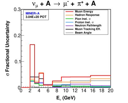
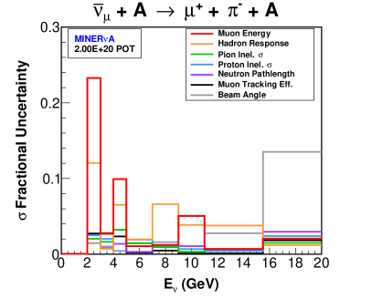
Figure 39: The fractional detector model uncertainties on the measured $\nu_{\mu}$ (left) and $\overline{\nu}_{\mu}$ (right) $\sigma(E_{\nu})$.

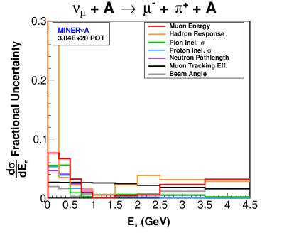
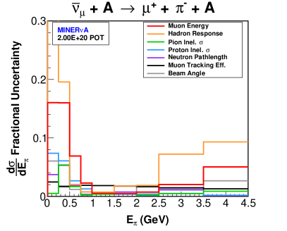
Figure 40: The fractional detector model uncertainties on the measured $\nu_{\mu}$ (left) and $\overline{\nu}_{\mu}$ (right) $\frac{d\sigma}{dE_{\pi}}$.

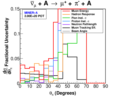
Figure 41: The fractional detector model uncertainties on the measured $\nu_{\mu}$ (left) and $\overline{\nu}_{\mu}$ (right) $\frac{d\sigma}{d\theta_{\pi}}$.

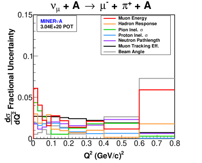
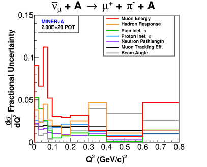
Figure 42: The fractional detector model uncertainties on the measured $\nu_{\mu}$ (left) and $\overline{\nu}_{\mu}$ (right) $\frac{d\sigma}{dQ^{2}}$.

XII.E.1 Muon Tracking Efficiency

The MC was weighted to correct the difference between MC and the data in the efficiency of tracking the muon in MINOS due to pile-up not being simulated in MINOS. An uncertainty on the correction to the MC tracking efficiency was included in the cross section results, which was evaluated by varying the size of the corrections by $\pm$50% of their values.

XII.E.2 Muon Energy Scale

Systematic uncertainty on the reconstructed muon energy affects the reconstructed values of other kinematic parameters, as well as the signal and background coherent candidate event rates via the cuts on $E_{\nu}$ and $|t|$. The muon energy uncertainty consists of uncertainties on the MINOS track momentum and the muon energy loss within MINERvA.

The momentum of a tracked muon in MINOS is measured by either the range of the track or its curvature in the magnetic field, with the range measurement being more precise. The range measurement uncertainty was estimated to be 2%, and consists of uncertainties on the MINOS geometry and material models, muon energy loss calculation, and track vertex reconstruction bib:minos_nim . The curvature measurement uncertainty was estimated using a high-statistics sample of muons produced upstream of the detector that enter the front face of MINOS and stop in its fully instrumented region. The difference between the data and MC distribution means established a 0.6% (2.5%) uncertainty on the curvature measurement beyond the 2% uncertainty on the range measurement for muon momentum above (below) 1 GeV/c. The uncertainties were added in quadrature to give an estimated curvature measurement uncertainty of 2.1% (3.1%) for muon momentum above (below) 1 GeV/c.

The uncertainty on the muon energy loss in MINERvA consisted of uncertainties on the MINERvA material assay and the Bethe-Bloch energy loss prediction. The effects of the material assay uncertainties were estimated by varying the detector mass in the muon energy loss calculation. The uncertainty on the Bethe-Bloch energy loss prediction was estimated by comparing the Bethe-Bloch muon range prediction to the Groom muon range tables bib:muon_range_tables for the materials in the MINERvA detector. For muons originating in the tracker and exiting the back of MINERvA, the effects of the material assay and Bethe-Bloch prediction uncertainties on the muon energy loss were estimated to be 11 MeV and 30 MeV on average, respectively.

For each event, the reconstructed muon energy uncertainty $\Delta$$E_{\mu}$ was the quadrature sum of the MINOS track momentum and MINERvA muon energy loss uncertainties. The muon energy uncertainty on the cross sections was evaluated by varying the muon energy in the MC by $\pm\Delta$$E_{\mu}$.

XII.E.3 Pion and Proton Response

The calorimetric correction for reconstructing $E_{\pi}$ from the visible energy was tuned to the simulated response to pions. This uncertainty was constrained by measurements of the single pion and proton response in the MINERvA test beam data and MC bib:test_beam . The response for each pion and proton event was measured as the ratio of the visible energy to the incoming particle energy, and the detector MC agreed with the data in the mean pion (proton) response to within 5% (3%) over the sampled incoming energy range. This difference was used to evaluate the systematic uncertainty.

XII.E.4 Pion & Proton Interaction Cross Section

The interaction of pions and protons within MINERvA affects the tracking efficiency, angular resolution, vertex energy and calorimetric response for both pions and protons, as well as the proton score. The uncertainty on the measured coherent cross sections due to the uncertainty in pion and proton interaction rates in the MC was evaluated by varying the rate of pion and proton inelastic scattering on carbon in the MC by $\pm$10%. Here, inelastic scattering includes charge exchange and absorption processes. The size of the variation, referred to as $\delta$ below was determined from comparisons of Geant4 to hadron scattering data Ashery et al. (1981); Allardyce et al. (1973); Saunders et al. (1996); Lee and Redwine (2002); Abfalterer et al. (2001); Schimmerling et al. (1973); Voss and Wilson (1956); Slypen et al. (1995); Franz et al. (1990); Tippawan et al. (2009); Bevilacqua et al. (2013); Zanelli et al. (1981). The inelastic scattering rate was varied using an event-by-event weighting technique where a weight was calculated for each final state pion and proton. The weight for a pion or proton that interacted inelastically was calculated as

$$W_{inel}=\frac{1-e^{-\rho x\sigma_{inel}(1+\delta)}}{1-e^{-\rho x\sigma_{inel}}},$$ (23)

and the weight for a pion/proton that did not interact inelastically was calculated as

$$W_{non-inel}=\frac{e^{-\rho x\sigma_{inel}(1+\delta)}}{e^{-\rho x\sigma_{inel}}}=e^{-\rho x\sigma_{inel}\delta},$$ (24)

where $\rho$ is the average density of the scintillator planes, $x$ is the total path length of the particle, $\sigma_{inel}$ is the energy averaged pion or proton inelastic scattering cross section on carbon, and $\delta$ is the variation on the inelastic scattering rate. The energy averaged cross section was used in calculating the weights to account for the dependence of the cross section on pion or proton energy, and was calculated as

$$\sigma_{inel}=\frac{1}{E_{f}-E_{i}}\int_{E_{i}}^{E_{f}}\sigma_{inel}(E)dE,$$ (25)

where $E_{i}$ and $E_{f}$ are the initial and final kinetic energy of the pion or proton, respectively, and $\sigma_{inel}(E)$ is a parameterization of the pion or proton inelastic scattering cross section on carbon from the hadron scattering data. The weight for each MC event was the product of the weights for all final state pions and protons. The event weights were normalized to preserve the total neutrino interaction rate for each MC event category.

The pion and proton calorimetric response uncertainties from the test beam measurements include uncertainties on the pion and proton interaction rates. The separate evaluation of the interaction rate uncertainties here double counts their contribution to the calorimetric response uncertainties. Since it is difficult in practice to isolate their contribution to the calorimetric response uncertainties, the best approach is to conservatively include the pion and proton interaction rate uncertainties on the calorimetric response along with the calorimetric response uncertainties from the test beam measurements.

XII.E.5 Neutron Path Length

In MINERvA, neutrons tend to either exit the detector without depositing any energy or deposit only a small fraction of their energy via a hadronic interaction. The neutron interaction rate therefore has a small effect on the calorimetric response. However, final state neutrons that promptly interact can affect the vertex energy and occasionally produce a tracked proton or pion. The neutron interaction rate therefore affects the predicted rate of background coherent candidates.

The uncertainty in the measured coherent cross sections due to the uncertainty on the neutron interaction rate in the MC was evaluated by varying the neutron mean free path, similar to the procedure in Sec. XII.E.4. The mean free path was varied $\pm$25% for neutron kinetic energy below 40 MeV, $\pm$10% between 50 and 150 MeV, and $\pm$20% above 300 MeV with interpolations in the uncertainties between these regions. The amount of these variations was determined from comparisons of GEANT4 and neutron scattering data.

XII.E.6 Beam Direction

Reconstruction of event kinematics assumed the incoming neutrino direction was parallel to the neutrino beam axis. The measured cross sections are therefore sensitive to uncertainty on the beam direction. The measurement of the beam direction using the $\nu_{\mu}$ and $\overline{\nu}_{\mu}$ CC low-$\nu$ samples agreed with the beam direction in the model of the detector geometry to within $\sim$3 mrad in both the vertical (YZ) and horizontal (XZ) planes. The uncertainty in the cross sections from beam direction uncertainty was evaluated by varying the beam direction $\pm$3 mrad in both the vertical and horizontal planes.

XIII Measured Cross Sections

The measured $\nu_{\mu}$ and $\overline{\nu}_{\mu}$ cross sections are shown in Figs. 43–46 along with cross section predictions from GENIE 2.8.4 in the default Rein-Sehgal model and the alternate Berger-Sehgal model. The $\chi^{2}$ for the comparison of each measured cross section to the GENIE Rein-Sehgal and Berger-Sehgal predictions is listed in Table 9. The $\chi^{2}$ was calculated as

$$\chi^{2}=AC^{-1}A^{T},$$ (26)

where $C$ is the bin-to-bin covariance matrix for the total uncertainty (statistical + total systematic) on the measured cross section, and the elements of the vector $A$ are

$$A_{i}=\sigma^{meas}_{i}-\sigma^{pred}_{i},$$ (27)

where $\sigma^{meas}_{i}$ and $\sigma^{pred}_{i}$ are the measured and predicted cross sections in bin $i$, respectively.

Both the GENIE Rein-Sehgal and Berger-Sehgal predictions are consistent with the measured cross sections in overall rate. The Berger-Sehgal overall rate is lower than the Rein-Sehgal overall because of the lower Berger-Sehgal pion-carbon elastic scattering cross section in the delta resonance region. Both predictions differ in shape from the measured $\frac{d\sigma}{dE_{\pi}}$ and $\frac{d\sigma}{d\theta_{\pi}}$. Assuming the tested validity of PCAC, this suggests that both models mis-model the pion-carbon elastic scattering cross section. Both predictions agree in shape with the measured $\frac{d\sigma}{dQ^{2}}$, which supports the axial vector dipole parameterization of the $Q^{2}$ dependence of the coherent cross section.

The measured $\frac{d\sigma}{d\theta_{\pi}}$ for large $\theta_{\pi}$ are below zero because of background subtraction; however the size of the uncertainties and bin-to-bin correlations is such that these results are fully consistent with zero.

Tables with the cross section results and the relevant covariance matrices describing their uncertainties may be found in the Appendix.

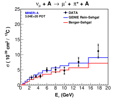
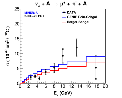
Figure 43: The measured $\sigma(E_{\nu})$ for the $\nu_{\mu}$ (left) and $\overline{\nu}_{\mu}$ (right), samples. The inner and outer error bars are the statistical and total (statistical + systematic) uncertainties, respectively.

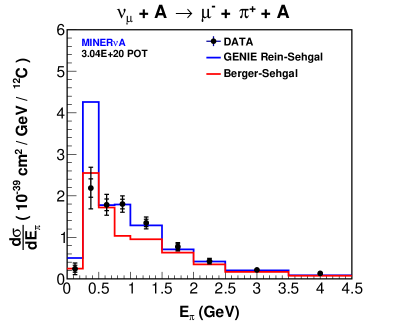
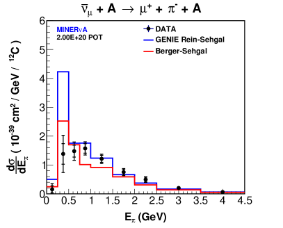
Figure 44: The measured $\frac{d\sigma}{dE_{\pi}}$ for the $\nu_{\mu}$ (left) and $\overline{\nu}_{\mu}$ (right) samples. The inner and outer error bars are the statistical and total (statistical + systematic) uncertainties, respectively.

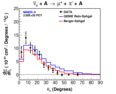
Figure 45: The measured $\frac{d\sigma}{d\theta_{\pi}}$ for the $\nu_{\mu}$ (left) and $\overline{\nu}_{\mu}$ (right) samples. The inner and outer error bars are the statistical and total (statistical + systematic) uncertainties, respectively.

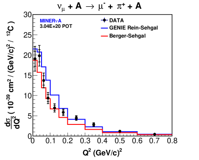
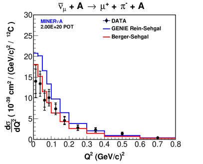
Figure 46: The measured $\frac{d\sigma}{dQ^{2}}$ for the $\nu_{\mu}$ (left) and $\overline{\nu}_{\mu}$ (right) samples. The inner and outer error bars are the statistical and total (statistical + systematic) uncertainties, respectively.

	$\nu_{\mu}\ \chi^{2}$		$\overline{\nu}_{\mu}\ \chi^{2}$
Cross section	RS	BS	RS	BS	NDF
$\sigma(E_{\nu})$	10.6	9.6	25.6	14.7	8
$d\sigma/dE_{\pi}$	46.2	58.7	35.8	40.4	9
$d\sigma/d\theta_{\pi}$	1164.5	171.9	122.2	29.1	12
$d\sigma/dQ^{2}$	19.3	13.5	16.2	11.4	10

Table 9: $\chi^{2}$ for the comparisons of the measured $\nu_{\mu}$ and $\overline{\nu}_{\mu}$ cross sections to the GENIE 2.8.4 Rein-Sehgal (RS) and Berger-Sehgal (BS) predictions

XIV $\nu_{\mu}$-$\overline{\nu}_{\mu}$ Cross Section Comparisons

The measured $\nu_{\mu}$ and $\overline{\nu}_{\mu}$ coherent cross sections may be compared to test the prediction of the PCAC coherent model (Sec. II.A) that the neutrino and antineutrino cross sections are equal for a particular $E_{\nu}$. The measured $\nu_{\mu}$ and $\overline{\nu}_{\mu}$ $\sigma(E_{\nu})$ can be compared directly in each $E_{\nu}$ bin. The measured $\nu_{\mu}$ and $\overline{\nu}_{\mu}$ flux integrated differential cross sections cannot be compared directly since they are integrated over different $E_{\nu}$ spectra. The effect of the different $E_{\nu}$ spectra on the $\nu_{\mu}$ and $\overline{\nu}_{\mu}$ differential cross sections predicted by the GENIE implementation of the Rein-Sehgal coherent model is illustrated in Fig. 47. The $\overline{\nu}_{\mu}$ flux is $\sim\frac{1}{2}$ the $\nu_{\mu}$ flux for 5 $<$ $E_{\nu}$ $<$ 20 GeV, which results in a lower $\overline{\nu}_{\mu}$ cross section at high-$E_{\pi}$, low-$\theta_{\pi}$, and high-$Q^{2}$.

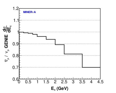
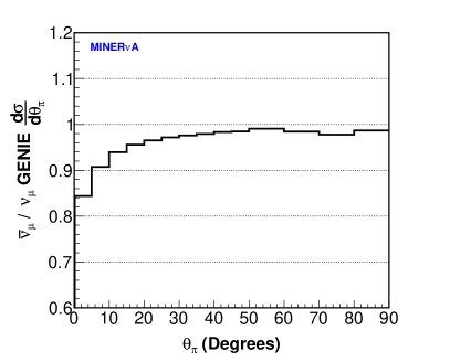
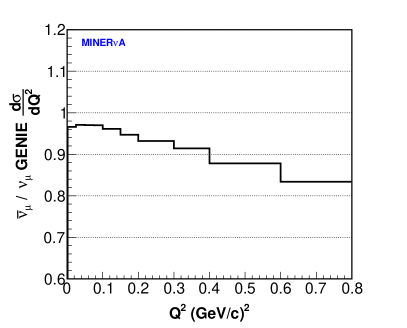
Figure 47: The ratio of the coherent differential cross sections predicted by GENIE for the $\overline{\nu}_{\mu}$ flux to that for the $\nu_{\mu}$ flux

To compare the measured $\nu_{\mu}$ and $\overline{\nu}_{\mu}$ differential cross sections, the $\nu_{\mu}$ cross sections are weighted to the $\overline{\nu}_{\mu}$ flux spectrum. The $\nu_{\mu}$ cross sections are weighted instead of the $\overline{\nu}_{\mu}$ cross sections to minimize amplifying statistical fluctuations. The approach employed was to weight the $\nu_{\mu}$ background subtracted coherent candidate event rates, unfolding matrices, efficiency corrections, and flux normalization to the $\overline{\nu}_{\mu}$ flux and remeasure the $\nu_{\mu}$ cross sections. The $\nu_{\mu}$ background subtracted coherent candidate event rate in reconstructed kinematic parameter bin $j$ was weighted as a function of reconstructed $E_{\nu}$ as

$$N_{j}^{data}-N_{j}^{bkgd}=\displaystyle\sum_{k}W_{k}^{reco}(N_{jk}^{data}-N_{jk}^{bkgd}),$$ (28)

where $W_{k}^{reco}$ is the weight for reconstructed $E_{\nu}$ bin $k$. $W_{k}^{reco}$ was calculated as

$$W_{k}^{reco}=\displaystyle\sum_{m}U_{km}^{\nu_{\mu}}\frac{\phi_{m}^{\overline{\nu}_{\mu}}}{\phi_{m}^{\nu_{\mu}}},$$ (29)

where $\phi_{m}^{\overline{\nu}_{\mu}}$ and $\phi_{m}^{\nu_{\mu}}$ are the $\overline{\nu}_{\mu}$ and $\nu_{\mu}$ fluxes per POT in true $E_{\nu}$ bin $m$, respectively, and $U_{km}^{\nu_{\mu}}$ is the $\nu_{\mu}$ $E_{\nu}$ unfolding matrix element normalized to give the estimated fraction of selected coherent events in reconstructed bin $k$ originating from true bin $m$. The $\nu_{\mu}$ unfolding matrices and efficiency corrections were weighted to the $\overline{\nu}_{\mu}$ flux by weighting each event in the $\nu_{\mu}$ signal-only MC sample by the flux ratio $\phi^{\overline{\nu}_{\mu}}/\phi^{\nu_{\mu}}$ for the event $E_{\nu}$ and recalculating the unfolding matrices and efficiency corrections. The $\nu_{\mu}$ flux was weighted as a function of $E_{\nu}$ by the flux ratio $\phi^{\overline{\nu}_{\mu}}(E_{\nu})/\phi^{\nu_{\mu}}(E_{\nu})$ and integrated to give the flux normalization for the weighted $\nu_{\mu}$ differential cross sections. The fractional systematic uncertainty on the weighted $\nu_{\mu}$ differential cross sections was forced to be equal to that on the unweighted cross sections by preserving the fractional difference of each systematic variation in the weighting. The ratio of the weighted to unweighted $\nu_{\mu}$ differential cross sections is shown in Fig. 47. For the remainder of this section, $\nu_{\mu}$ differential cross section refers to the $\nu_{\mu}$ differential cross section weighted to the $\overline{\nu}_{\mu}$ flux.

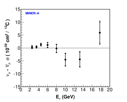
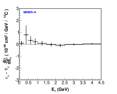
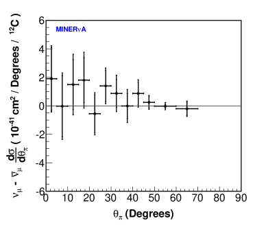
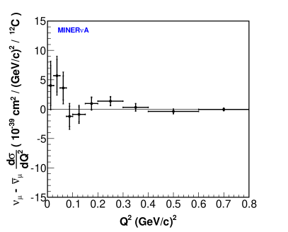
Figure 48: The measured $\overline{\nu}_{\mu}-\nu_{\mu}$ cross-section differences

The measured $\nu_{\mu}-\overline{\nu}_{\mu}$ cross-section differences are shown in Fig. 48. The uncertainties in the cross-section differences were calculated from the combined statistical and systematic covariance matrices for the $\nu_{\mu}$ and $\overline{\nu}_{\mu}$ cross sections. The combined statistical covariance matrix is the sum of the $\nu_{\mu}$ and $\overline{\nu}_{\mu}$ statistical covariance matrices. The elements of the combined covariance matrix for each systematic uncertainty $C^{sys}$ were calculated as

$$C^{sys}_{ij}=C^{\nu_{\mu}}_{ij}+C^{\overline{\nu}_{\mu}}_{ij}-C^{\nu_{\mu}\overline{\nu}_{\mu}}_{ij}-C^{\nu_{\mu}\overline{\nu}_{\mu}}_{ji},$$ (30)

where $C^{\nu_{\mu}}$ and $C^{\overline{\nu}_{\mu}}$ are the systematic covariance matrices for the $\nu_{\mu}$ and $\overline{\nu}_{\mu}$ cross sections, respectively, and $C^{\nu_{\mu}\overline{\nu}_{\mu}}$ is the joint systematic covariance matrix for the $\nu_{\mu}$ and $\overline{\nu}_{\mu}$ cross sections. The elements of $C^{\nu_{\mu}\overline{\nu}_{\mu}}$ were calculated as

$$C^{\nu_{\mu}\overline{\nu}_{\mu}}_{ij}=\frac{1}{N}\displaystyle\sum_{k}\Delta\sigma^{\nu_{\mu}}_{ik}\Delta\sigma^{\overline{\nu}_{\mu}}_{jk},$$ (31)

where $\Delta\sigma^{\nu_{\mu}}_{ik}$ ($\Delta\sigma^{\overline{\nu}_{\mu}}_{jk}$) is the change to the $\nu_{\mu}$ ($\overline{\nu}_{\mu}$) cross section in bin $i$ ($j$) for variation $k$, and $N$ is the number of variations from which the systematic uncertainty was evaluated. The $\chi^{2}$ for the deviation of each $\nu_{\mu}-\overline{\nu}_{\mu}$ cross-section difference from zero are listed in Table 10 and were calculated as

$$\chi^{2}=AC^{-1}A^{T},$$ (32)

where $C$ is the total covariance (statistical + total systematic) matrix for the cross-section difference and the elements of the vector $A$ are defined as

$$A_{i}=\sigma^{\nu_{\mu}}_{i}-\sigma^{\overline{\nu}_{\mu}}_{i},$$ (33)

where $\sigma^{\nu_{\mu}}_{i}$ and $\sigma^{\overline{\nu}_{\mu}}_{i}$ are the $\nu_{\mu}$ and $\overline{\nu}_{\mu}$ cross sections in bin $i$. The $\chi^{2}$ probabilities in Table 10 show that the deviation of the $\nu_{\mu}-\overline{\nu}_{\mu}$ cross-section differences from zero are not significant and are consistent with the prediction of the PCAC coherent models that the neutrino and antineutrino cross sections are equal.

Cross section	$\chi^{2}$	NDF	$\chi^{2}$ Probability
$\sigma{E_{\nu}}$	11.4	8	0.181
$d\sigma/dE_{\pi}$	5.5	9	0.791
$d\sigma/d\theta_{\pi}$	5.3	12	0.948
$d\sigma/dQ^{2}$	11.2	10	0.341

Table 10: The $\chi^{2}$, number of degrees of freedom (NDF), and $\chi^{2}$ probability for the deviation of the measured $\nu_{\mu}-\overline{\nu}_{\mu}$ cross-section differences from zero.

The primary sources of systematic uncertainties in the $\nu_{\mu}$- $\overline{\nu}_{\mu}$ cross-section differences are the flux, neutron FSI, and pion response. Flux predictions can be improved by measuring hadron production from a neutrino production target. The electron vs. photon separation capability of liquid argon detectors can also improve the flux constraint from an in situ measurement of neutrino-electron elastic scattering. Reductions in cross section and FSI uncertainties on the incoherent single pion production backgrounds can be achieved by leveraging existing and future exclusive measurements.

XV Conclusions

This paper has reported measurements of $\nu_{\mu}$ and $\overline{\nu}_{\mu}$ CC coherent pion production on carbon from MINERvA data. The cross sections were measured for neutrino energies in the range 2.0 $<$ $E_{\nu}$ $<$ 20 GeV, where $\langle E_{\nu}\rangle\approx$ 4 GeV. The measurements were made by isolating coherent interactions using the model independent experimental signature of CC coherent scattering, which consists of a charged lepton and pion in the forward direction, no evidence of nuclear breakup, and small $|t|$. A data-driven constraint on the background prediction was designed to minimize dependence on modeling nuclear effects which are poorly understood. Unambiguous signals of $\nu_{\mu}$ and $\overline{\nu}_{\mu}$ CC coherent pion production above the predicted background were observed at small $|t|$. The cross sections $\sigma(E_{\nu})$, $\frac{d\sigma}{dQ^{2}}$, $\frac{d\sigma}{dE_{\pi}}$ and $\frac{d\sigma}{d\theta_{\pi}}$ were measured for both $\nu_{\mu}$ and $\overline{\nu}_{\mu}$ CC coherent pion production. $E_{\nu}$, $Q^{2}$, $E_{\pi}$, $\theta_{\pi}$ and $|t|$ characterize the kinematics of coherent scattering completely.

The measured cross sections were compared to the Rein-Sehgal and Berger-Sehgal coherent models, which are both based on Adler’s PCAC theorem. The Rein-Sehgal model calculates the pion-nucleus elastic scattering cross section from pion-nucleon scattering data. The Berger-Sehgal model calculates the pion-nucleus scattering cross section from pion-carbon elastic scattering data and scales the cross section to other nuclei. Both the Rein-Sehgal and Berger Sehgal predictions agree with the measured total cross-section as a function of neutrino energy in the $\nu_{\mu}$ and $\overline{\nu}_{\mu}$ samples. For both $\nu_{\mu}$ and $\overline{\nu}_{\mu}$, the measured $\frac{d\sigma}{dE_{\pi}}$ ($\frac{d\sigma}{d\theta_{\pi}}$) exhibits a harder (more forward) spectrum than the Rein-Sehgal and Berger-Sehgal predictions, which suggests that both models miscalculate the pion-nucleus elastic scattering cross section. The Rein-Sehgal predictions were brought into better agreement with the measured $\frac{d\sigma}{dE_{\pi}}$ and $\frac{d\sigma}{d\theta_{\pi}}$ by weighting the predicted rate of interactions with $E_{\pi}<$ 500 MeV by 50%. For both $\nu_{\mu}$ and $\overline{\nu}_{\mu}$, the Rein-Sehgal and Berger-Sehgal predictions are similar in shape to the measured $\frac{d\sigma}{dQ^{2}}$, which supports the axial vector dipole parameterization of the $Q^{2}$ dependence of the coherent cross section.

PCAC coherent models assume coherent scattering is a purely axial vector process. PCAC coherent models therefore predict equal cross sections for neutrinos and antineutrinos. To test this prediction, the measured $\nu_{\mu}$ and $\overline{\nu}_{\mu}$ cross sections were compared, where the $\nu_{\mu}$ differential cross sections were weighted to the $\overline{\nu}_{\mu}$ flux. No significant differences between the $\nu_{\mu}$ and $\overline{\nu}_{\mu}$ cross sections were observed.

Since the MINERvA scintillator contains equal numbers of carbon and hydrogen atoms, diffractive pion production on hydrogen is a possible contribution to the measured cross sections. Diffractive pion production is indistinguishable from coherent pion production when the recoil proton is undetected. A search for diffractive pion production within the coherent pion production candidate samples was performed by looking for ionization from a recoil proton near the interaction vertex. Neither the $\nu_{\mu}$ nor $\overline{\nu}_{\mu}$ coherent candidate samples exhibited evidence for such a diffractive contribution.

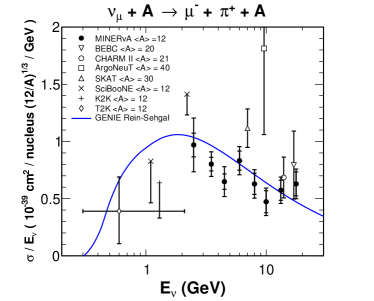
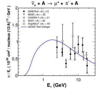
Figure 49: Compilation of measurements of the $\nu_{\mu}$ (top) and $\overline{\nu}_{\mu}$ (bottom) CC coherent pion production cross sections as a function of energy. Cross sections divided by neutrino energy is shown for display convenience. All results are scaled to A=12 (carbon) assuming $\sigma\propto A^{1/3}$.

The measurements reported in this paper are a significant addition to the world data set of neutrino-nucleus coherent pion production. Cross sections as a function of neutrino energy from the world data set are shown in Fig. 49. This includes recent measurements from ArgoNEUT bib:coh_cc_argo and T2K bib:coh_cc_t2k which are significantly less precise than the MINERvA measurements and do not report differential cross sections. The T2K measurement, however, plays a special role here in that it shows consistency of the cross section at lower energies than accessible by MINERvA with the $d\sigma/dE_{\pi}$ at low pion energies below the prediction of the GENIE Rein-Sehgal model.

The MINERvA measurements presented in this paper provide the most precise information about charged-current coherent pion production below neutrino energies of 15 GeV. The measurements provide constraints on not only the total rate, but also on the kinematics of coherent pion production. These measurements can be used to benchmark coherent pion production models from production threshold up to neutrino energies of 20 GeV, which is the most important energy regime for current and future neutrino oscillation experiments.

Cross Section Results and Covariance Matrices

	$\sigma(E_{\nu})\ \ (\text{cm}^{2}/^{12}\text{C})\times 10^{-39}$	$\sigma(E_{\nu})\ \ (\text{cm}^{2}/^{12}\text{C})\times 10^{-39}$
$E_{\nu}$  (GeV)	$\nu_{\mu}$	$\overline{\nu}_{\mu}$
2.0 - 3.0	2.424 $\pm$ 0.258 $\pm$ 0.221 $\pm$ 0.479	2.105 $\pm$ 0.385 $\pm$ 0.214 $\pm$ 0.630
3.0 - 4.0	2.806 $\pm$ 0.207 $\pm$ 0.187 $\pm$ 0.255	2.418 $\pm$ 0.301 $\pm$ 0.156 $\pm$ 0.268
4.0 - 5.0	2.920 $\pm$ 0.300 $\pm$ 0.379 $\pm$ 0.336	1.621 $\pm$ 0.386 $\pm$ 0.272 $\pm$ 0.316
5.0 - 7.0	4.994 $\pm$ 0.501 $\pm$ 0.472 $\pm$ 0.276	3.828 $\pm$ 0.785 $\pm$ 0.436 $\pm$ 0.372
7.0 - 9.0	5.031 $\pm$ 0.738 $\pm$ 0.573 $\pm$ 0.344	5.212 $\pm$ 1.330 $\pm$ 0.569 $\pm$ 0.512
9.0 - 11.0	4.728 $\pm$ 0.970 $\pm$ 0.587 $\pm$ 0.397	9.241 $\pm$ 2.158 $\pm$ 0.886 $\pm$ 0.883
11.0 - 15.5	7.599 $\pm$ 1.159 $\pm$ 0.810 $\pm$ 0.567	12.000 $\pm$ 2.555 $\pm$ 1.092 $\pm$ 0.941
15.5 - 20.0	11.169 $\pm$ 1.856 $\pm$ 1.109 $\pm$ 0.796	5.243 $\pm$ 3.631 $\pm$ 0.827 $\pm$ 1.547

Table 11: The measurement of the cross section as a function of $E_{\nu}$ with statistical, flux systematic, and non-flux systematic uncertainties

	$d\sigma/dE_{\pi}\ \ (\text{cm}^{2}/\text{GeV}/^{12}\text{C})\times 10^{-39}$	$d\sigma/dE_{\pi}\ \ (\text{cm}^{2}/\text{GeV}/^{12}\text{C})\times 10^{-39}$
$E_{\pi}$  (GeV)	$\nu_{\mu}$	$\overline{\nu}_{\mu}$
0 - 0.25	0.242 $\pm$ 0.084 $\pm$ 0.015 $\pm$ 0.110	0.156 $\pm$ 0.125 $\pm$ 0.012 $\pm$ 0.153
0.25 - 0.5	2.186 $\pm$ 0.222 $\pm$ 0.133 $\pm$ 0.429	1.383 $\pm$ 0.356 $\pm$ 0.062 $\pm$ 0.536
0.5 - 0.75	1.783 $\pm$ 0.140 $\pm$ 0.110 $\pm$ 0.179	1.478 $\pm$ 0.205 $\pm$ 0.079 $\pm$ 0.229
0.75 - 1.0	1.802 $\pm$ 0.115 $\pm$ 0.111 $\pm$ 0.116	1.574 $\pm$ 0.164 $\pm$ 0.098 $\pm$ 0.126
1.0 - 1.5	1.347 $\pm$ 0.089 $\pm$ 0.084 $\pm$ 0.075	1.214 $\pm$ 0.121 $\pm$ 0.083 $\pm$ 0.069
1.5 - 2.0	0.773 $\pm$ 0.072 $\pm$ 0.048 $\pm$ 0.048	0.753 $\pm$ 0.098 $\pm$ 0.054 $\pm$ 0.047
2.0 - 2.5	0.427 $\pm$ 0.052 $\pm$ 0.025 $\pm$ 0.034	0.495 $\pm$ 0.084 $\pm$ 0.035 $\pm$ 0.038
2.5 - 3.5	0.214 $\pm$ 0.033 $\pm$ 0.012 $\pm$ 0.022	0.203 $\pm$ 0.049 $\pm$ 0.013 $\pm$ 0.026
3.5 - 4.5	0.131 $\pm$ 0.023 $\pm$ 0.007 $\pm$ 0.014	0.062 $\pm$ 0.021 $\pm$ 0.004 $\pm$ 0.011

Table 12: The measurement of the differential cross section as a function of pion energy, $d\sigma/dE_{\pi}$, with statistical, flux systematic, and non-flux systematic uncertainties

	$d\sigma/d\theta_{\pi}\ \ (\text{cm}^{2}/\text{Degree}/^{12}\text{C})\times 10^{-41}$	$d\sigma/d\theta_{\pi}\ \ (\text{cm}^{2}/\text{Degree}/^{12}\text{C})\times 10^{-41}$
$\theta_{\pi}$ (Degrees)	$\nu_{\mu}$	$\overline{\nu}_{\mu}$
0 - 5	12.703 $\pm$ 1.380 $\pm$ 0.814 $\pm$ 0.815	8.505 $\pm$ 1.880 $\pm$ 0.668 $\pm$ 0.710
5 - 10	15.161 $\pm$ 1.298 $\pm$ 0.938 $\pm$ 1.317	13.908 $\pm$ 1.779 $\pm$ 0.974 $\pm$ 0.930
10 - 15	12.032 $\pm$ 1.016 $\pm$ 0.734 $\pm$ 0.559	10.175 $\pm$ 1.450 $\pm$ 0.665 $\pm$ 1.160
15 - 20	11.256 $\pm$ 0.900 $\pm$ 0.690 $\pm$ 0.576	9.056 $\pm$ 1.313 $\pm$ 0.571 $\pm$ 1.116
20 - 25	7.385 $\pm$ 0.723 $\pm$ 0.447 $\pm$ 0.527	7.498 $\pm$ 1.146 $\pm$ 0.466 $\pm$ 0.584
25 - 30	5.166 $\pm$ 0.628 $\pm$ 0.312 $\pm$ 0.515	3.746 $\pm$ 0.901 $\pm$ 0.197 $\pm$ 0.571
30 - 35	3.434 $\pm$ 0.565 $\pm$ 0.207 $\pm$ 0.768	2.582 $\pm$ 0.800 $\pm$ 0.129 $\pm$ 0.408
35 - 40	1.735 $\pm$ 0.462 $\pm$ 0.103 $\pm$ 0.673	1.653 $\pm$ 0.772 $\pm$ 0.071 $\pm$ 0.464
40 - 45	1.586 $\pm$ 0.467 $\pm$ 0.094 $\pm$ 0.496	0.655 $\pm$ 0.630 $\pm$ 0.045 $\pm$ 0.363
45 - 50	0.245 $\pm$ 0.301 $\pm$ 0.013 $\pm$ 0.368	-0.072 $\pm$ 0.286 $\pm$ 0.039 $\pm$ 0.211
50 - 60	-0.074 $\pm$ 0.036 $\pm$ 0.006 $\pm$ 0.036	-0.046 $\pm$ 0.107 $\pm$ 0.056 $\pm$ 0.220
60 - 70	-0.085 $\pm$ 0.036 $\pm$ 0.006 $\pm$ 0.026	0.117 $\pm$ 0.458 $\pm$ 0.042 $\pm$ 0.276

Table 13: The measurement of the differential cross section as a function of pion angle, $d\sigma/d\theta_{\pi}$, with statistical, flux systematic, and non-flux systematic uncertainties

	$d\sigma/dQ^{2}\ \ (\text{cm}^{2}/(\text{GeV}/\text{c})^{2}/^{12}\text{C})\times 10^{-39}$	$d\sigma/dQ^{2}\ \ (\text{cm}^{2}/(\text{GeV}/\text{c})^{2}/^{12}\text{C})\times 10^{-39}$
$Q^{2}$ (GeV/c)2	$\nu_{\mu}$	$\overline{\nu}_{\mu}$
0 - 0.025	19.068 $\pm$ 1.848 $\pm$ 1.188 $\pm$ 2.119	14.004 $\pm$ 2.909 $\pm$ 0.794 $\pm$ 2.481
0.025 - 0.05	19.812 $\pm$ 1.519 $\pm$ 1.242 $\pm$ 1.629	13.421 $\pm$ 2.303 $\pm$ 0.792 $\pm$ 1.805
0.05 - 0.075	13.713 $\pm$ 1.149 $\pm$ 0.857 $\pm$ 1.163	9.445 $\pm$ 1.681 $\pm$ 0.558 $\pm$ 1.672
0.075 - 0.1	9.375 $\pm$ 0.886 $\pm$ 0.585 $\pm$ 0.896	10.049 $\pm$ 1.493 $\pm$ 0.609 $\pm$ 1.187
0.1 - 0.15	6.951 $\pm$ 0.647 $\pm$ 0.431 $\pm$ 0.665	7.370 $\pm$ 1.096 $\pm$ 0.428 $\pm$ 0.816
0.15 - 0.2	5.844 $\pm$ 0.554 $\pm$ 0.361 $\pm$ 0.467	4.559 $\pm$ 0.825 $\pm$ 0.258 $\pm$ 0.528
0.2 - 0.3	4.444 $\pm$ 0.422 $\pm$ 0.274 $\pm$ 0.289	2.827 $\pm$ 0.571 $\pm$ 0.171 $\pm$ 0.316
0.3 - 0.4	2.825 $\pm$ 0.364 $\pm$ 0.172 $\pm$ 0.214	2.282 $\pm$ 0.486 $\pm$ 0.152 $\pm$ 0.232
0.4 - 0.6	1.186 $\pm$ 0.226 $\pm$ 0.068 $\pm$ 0.138	1.402 $\pm$ 0.333 $\pm$ 0.093 $\pm$ 0.114
0.6 - 0.8	0.432 $\pm$ 0.149 $\pm$ 0.021 $\pm$ 0.092	0.396 $\pm$ 0.187 $\pm$ 0.023 $\pm$ 0.074

Table 14: The measurement of the differential cross section as a function of $Q^{2}$, $d\sigma/dQ^{2}$, with statistical, flux systematic, and non-flux systematic uncertainties

$E_{\nu}$  (GeV)	$(\nu_{\mu}/\text{cm}^{2}/\text{POT})\times 10^{-8}$	$(\overline{\nu}_{\mu}/\text{cm}^{2}/\text{POT})\times 10^{-8}$
2.0 - 3.0	0.742	0.663
3.0 - 4.0	0.767	0.645
4.0 - 5.0	0.313	0.244
5.0 - 7.0	0.189	0.130
7.0 - 9.0	0.098	0.055
9.0 - 11.0	0.065	0.033
11.0 - 15.5	0.077	0.035
15.5 - 20.0	0.044	0.018

Table 15: $\nu_{\mu}$ and $\overline{\nu}_{\mu}$ fluxes

	$\sigma(E_{\nu})\ \ (\text{cm}^{2}/^{12}\text{C})\times 10^{-39}$	$\sigma(E_{\nu})\ \ (\text{cm}^{2}/^{12}\text{C})\times 10^{-39}$	$\sigma(E_{\nu})\ \ (\text{cm}^{2}/^{12}\text{C})\times 10^{-39}$
$E_{\nu}$  (GeV)	$\nu_{\mu}$	$\overline{\nu}_{\mu}$	$\nu_{\mu}-\overline{\nu}_{\mu}$
2.0 - 3.0	2.424 $\pm$ 0.258 $\pm$ 0.221 $\pm$ 0.479	2.105 $\pm$ 0.385 $\pm$ 0.214 $\pm$ 0.630	0.319 $\pm$ 0.464 $\pm$ 0.146 $\pm$ 0.381
3.0 - 4.0	2.806 $\pm$ 0.207 $\pm$ 0.187 $\pm$ 0.255	2.418 $\pm$ 0.301 $\pm$ 0.156 $\pm$ 0.268	0.388 $\pm$ 0.365 $\pm$ 0.132 $\pm$ 0.259
4.0 - 5.0	2.920 $\pm$ 0.300 $\pm$ 0.379 $\pm$ 0.336	1.621 $\pm$ 0.386 $\pm$ 0.272 $\pm$ 0.316	1.299 $\pm$ 0.489 $\pm$ 0.170 $\pm$ 0.260
5.0 - 7.0	4.994 $\pm$ 0.501 $\pm$ 0.472 $\pm$ 0.276	3.828 $\pm$ 0.785 $\pm$ 0.436 $\pm$ 0.372	1.166 $\pm$ 0.931 $\pm$ 0.347 $\pm$ 0.344
7.0 - 9.0	5.031 $\pm$ 0.738 $\pm$ 0.573 $\pm$ 0.344	5.212 $\pm$ 1.330 $\pm$ 0.569 $\pm$ 0.512	-0.182 $\pm$ 1.521 $\pm$ 0.401 $\pm$ 0.539
9.0 - 11.0	4.728 $\pm$ 0.970 $\pm$ 0.587 $\pm$ 0.397	9.241 $\pm$ 2.158 $\pm$ 0.886 $\pm$ 0.883	-4.513 $\pm$ 2.366 $\pm$ 0.582 $\pm$ 0.668
11.0 - 15.5	7.599 $\pm$ 1.159 $\pm$ 0.810 $\pm$ 0.567	12.000 $\pm$ 2.555 $\pm$ 1.092 $\pm$ 0.941	-4.401 $\pm$ 2.805 $\pm$ 0.763 $\pm$ 0.894
15.5 - 20.0	11.169 $\pm$ 1.856 $\pm$ 1.109 $\pm$ 0.796	5.243 $\pm$ 3.631 $\pm$ 0.827 $\pm$ 1.547	5.925 $\pm$ 4.078 $\pm$ 0.956 $\pm$ 1.669

Table 16: The measurement of the cross section as a function of $E_{\nu}$ with statistical, flux systematic, and non-flux systematic uncertainties for $\nu_{\mu}$, $\overline{\nu}_{\mu}$, and the difference between $\nu_{\mu}$ and $\overline{\nu}_{\mu}$

	$d\sigma/dE_{\pi}\ \ (\text{cm}^{2}/\text{GeV}/^{12}\text{C})\times 10^{-39}$	$d\sigma/dE_{\pi}\ \ (\text{cm}^{2}/\text{GeV}/^{12}\text{C})\times 10^{-39}$	$d\sigma/dE_{\pi}\ \ (\text{cm}^{2}/\text{GeV}/^{12}\text{C})\times 10^{-39}$
$E_{\pi}$  (GeV)	$\nu_{\mu}$	$\overline{\nu}_{\mu}$	$\nu_{\mu}-\overline{\nu}_{\mu}$
0 - 0.25	0.241 $\pm$ 0.085 $\pm$ 0.015 $\pm$ 0.110	0.156 $\pm$ 0.125 $\pm$ 0.012 $\pm$ 0.153	0.086 $\pm$ 0.151 $\pm$ 0.011 $\pm$ 0.071
0.25 - 0.5	2.173 $\pm$ 0.224 $\pm$ 0.132 $\pm$ 0.426	1.383 $\pm$ 0.356 $\pm$ 0.062 $\pm$ 0.536	0.790 $\pm$ 0.421 $\pm$ 0.112 $\pm$ 0.637
0.5 - 0.75	1.800 $\pm$ 0.141 $\pm$ 0.110 $\pm$ 0.180	1.478 $\pm$ 0.205 $\pm$ 0.079 $\pm$ 0.229	0.321 $\pm$ 0.249 $\pm$ 0.084 $\pm$ 0.199
0.75 - 1.0	1.781 $\pm$ 0.114 $\pm$ 0.110 $\pm$ 0.114	1.574 $\pm$ 0.164 $\pm$ 0.098 $\pm$ 0.126	0.207 $\pm$ 0.200 $\pm$ 0.086 $\pm$ 0.102
1.0 - 1.5	1.295 $\pm$ 0.086 $\pm$ 0.081 $\pm$ 0.073	1.214 $\pm$ 0.121 $\pm$ 0.083 $\pm$ 0.069	0.081 $\pm$ 0.149 $\pm$ 0.066 $\pm$ 0.040
1.5 - 2.0	0.724 $\pm$ 0.068 $\pm$ 0.045 $\pm$ 0.048	0.753 $\pm$ 0.098 $\pm$ 0.054 $\pm$ 0.047	-0.029 $\pm$ 0.119 $\pm$ 0.040 $\pm$ 0.049
2.0 - 2.5	0.386 $\pm$ 0.047 $\pm$ 0.023 $\pm$ 0.033	0.495 $\pm$ 0.084 $\pm$ 0.035 $\pm$ 0.038	-0.108 $\pm$ 0.096 $\pm$ 0.026 $\pm$ 0.033
2.5 - 3.5	0.179 $\pm$ 0.027 $\pm$ 0.010 $\pm$ 0.019	0.203 $\pm$ 0.049 $\pm$ 0.013 $\pm$ 0.026	-0.024 $\pm$ 0.056 $\pm$ 0.011 $\pm$ 0.020
3.5 - 4.5	0.094 $\pm$ 0.017 $\pm$ 0.005 $\pm$ 0.011	0.062 $\pm$ 0.021 $\pm$ 0.004 $\pm$ 0.011	0.031 $\pm$ 0.027 $\pm$ 0.004 $\pm$ 0.008

Table 17: The measurement of the differential cross section as a function of pion energy, $d\sigma/dE_{\pi}$, with statistical, flux systematic, and non-flux systematic uncertainties for $\nu_{\mu}$, $\overline{\nu}_{\mu}$, and the difference between $\nu_{\mu}$ and $\overline{\nu}_{\mu}$. Note that the $\nu_{\mu}$ cross section is weighted to the $\overline{\nu}_{\mu}$ flux for calculating the cross section difference.

	$d\sigma/d\theta_{\pi}\ \ (\text{cm}^{2}/\text{Degree}/^{12}\text{C})\times 10^{-41}$	$d\sigma/d\theta_{\pi}\ \ (\text{cm}^{2}/\text{Degree}/^{12}\text{C})\times 10^{-41}$	$d\sigma/d\theta_{\pi}\ \ (\text{cm}^{2}/\text{Degree}/^{12}\text{C})\times 10^{-41}$
$\theta_{\pi}$ (Degrees)	$\nu_{\mu}$	$\overline{\nu}_{\mu}$	$\nu_{\mu}-\overline{\nu}_{\mu}$
0 - 5	10.402 $\pm$ 1.190 $\pm$ 0.663 $\pm$ 0.682	8.505 $\pm$ 1.880 $\pm$ 0.668 $\pm$ 0.710	1.897 $\pm$ 2.225 $\pm$ 0.537 $\pm$ 0.445
5 - 10	13.887 $\pm$ 1.197 $\pm$ 0.859 $\pm$ 1.206	13.908 $\pm$ 1.779 $\pm$ 0.974 $\pm$ 0.930	-0.021 $\pm$ 2.144 $\pm$ 0.742 $\pm$ 0.559
10 - 15	11.669 $\pm$ 0.969 $\pm$ 0.712 $\pm$ 0.553	10.175 $\pm$ 1.450 $\pm$ 0.665 $\pm$ 1.160	1.494 $\pm$ 1.744 $\pm$ 0.562 $\pm$ 1.087
15 - 20	10.859 $\pm$ 0.860 $\pm$ 0.666 $\pm$ 0.565	9.056 $\pm$ 1.313 $\pm$ 0.571 $\pm$ 1.116	1.803 $\pm$ 1.570 $\pm$ 0.517 $\pm$ 1.055
20 - 25	6.943 $\pm$ 0.686 $\pm$ 0.420 $\pm$ 0.502	7.498 $\pm$ 1.146 $\pm$ 0.466 $\pm$ 0.584	-0.555 $\pm$ 1.336 $\pm$ 0.365 $\pm$ 0.537
25 - 30	5.145 $\pm$ 0.618 $\pm$ 0.311 $\pm$ 0.515	3.746 $\pm$ 0.901 $\pm$ 0.197 $\pm$ 0.571	1.398 $\pm$ 1.093 $\pm$ 0.238 $\pm$ 0.577
30 - 35	3.454 $\pm$ 0.564 $\pm$ 0.207 $\pm$ 0.771	2.582 $\pm$ 0.800 $\pm$ 0.129 $\pm$ 0.408	0.872 $\pm$ 0.979 $\pm$ 0.168 $\pm$ 0.806
35 - 40	1.642 $\pm$ 0.450 $\pm$ 0.097 $\pm$ 0.628	1.653 $\pm$ 0.772 $\pm$ 0.071 $\pm$ 0.464	-0.011 $\pm$ 0.894 $\pm$ 0.091 $\pm$ 0.734
40 - 45	1.524 $\pm$ 0.466 $\pm$ 0.091 $\pm$ 0.459	0.655 $\pm$ 0.630 $\pm$ 0.045 $\pm$ 0.363	0.869 $\pm$ 0.783 $\pm$ 0.110 $\pm$ 0.562
45 - 50	0.174 $\pm$ 0.272 $\pm$ 0.010 $\pm$ 0.258	-0.072 $\pm$ 0.286 $\pm$ 0.039 $\pm$ 0.211	0.247 $\pm$ 0.395 $\pm$ 0.046 $\pm$ 0.290
50 - 60	-0.067 $\pm$ 0.042 $\pm$ 0.005 $\pm$ 0.032	-0.046 $\pm$ 0.107 $\pm$ 0.056 $\pm$ 0.220	-0.021 $\pm$ 0.115 $\pm$ 0.057 $\pm$ 0.219
60 - 70	-0.086 $\pm$ 0.039 $\pm$ 0.006 $\pm$ 0.026	0.117 $\pm$ 0.458 $\pm$ 0.042 $\pm$ 0.276	-0.203 $\pm$ 0.460 $\pm$ 0.042 $\pm$ 0.281

Table 18: The measurement of the differential cross section as a function of pion angle, $d\sigma/d\theta_{\pi}$, with statistical, flux systematic, and non-flux systematic uncertainties for $\nu_{\mu}$, $\overline{\nu}_{\mu}$, and the difference between $\nu_{\mu}$ and $\overline{\nu}_{\mu}$. Note that the $\nu_{\mu}$ cross section is weighted to the $\overline{\nu}_{\mu}$ flux for calculating the cross section difference.

	$d\sigma/dQ^{2}\ \ (\text{cm}^{2}/(\text{GeV}/\text{c})^{2}/^{12}\text{C})\times 10^{-39}$	$d\sigma/dQ^{2}\ \ (\text{cm}^{2}/(\text{GeV}/\text{c})^{2}/^{12}\text{C})\times 10^{-39}$	$d\sigma/dQ^{2}\ \ (\text{cm}^{2}/(\text{GeV}/\text{c})^{2}/^{12}\text{C})\times 10^{-39}$
$Q^{2}$ (GeV/c)2	$\nu_{\mu}$	$\overline{\nu}_{\mu}$	$\nu_{\mu}-\overline{\nu}_{\mu}$
0 - 0.025	18.019 $\pm$ 1.812 $\pm$ 1.121 $\pm$ 2.022	14.004 $\pm$ 2.909 $\pm$ 0.794 $\pm$ 2.481	4.015 $\pm$ 3.427 $\pm$ 0.843 $\pm$ 2.175
0.025 - 0.05	19.114 $\pm$ 1.529 $\pm$ 1.196 $\pm$ 1.576	13.421 $\pm$ 2.303 $\pm$ 0.792 $\pm$ 1.805	5.694 $\pm$ 2.765 $\pm$ 0.897 $\pm$ 1.599
0.05 - 0.075	13.047 $\pm$ 1.163 $\pm$ 0.814 $\pm$ 1.109	9.445 $\pm$ 1.681 $\pm$ 0.558 $\pm$ 1.672	3.602 $\pm$ 2.044 $\pm$ 0.616 $\pm$ 1.679
0.075 - 0.1	8.812 $\pm$ 0.886 $\pm$ 0.548 $\pm$ 0.849	10.049 $\pm$ 1.493 $\pm$ 0.609 $\pm$ 1.187	-1.237 $\pm$ 1.736 $\pm$ 0.476 $\pm$ 1.266
0.1 - 0.15	6.471 $\pm$ 0.647 $\pm$ 0.401 $\pm$ 0.627	7.370 $\pm$ 1.096 $\pm$ 0.428 $\pm$ 0.816	-0.899 $\pm$ 1.273 $\pm$ 0.337 $\pm$ 0.802
0.15 - 0.2	5.504 $\pm$ 0.555 $\pm$ 0.339 $\pm$ 0.447	4.559 $\pm$ 0.825 $\pm$ 0.258 $\pm$ 0.528	0.945 $\pm$ 0.995 $\pm$ 0.253 $\pm$ 0.460
0.2 - 0.3	4.186 $\pm$ 0.420 $\pm$ 0.258 $\pm$ 0.271	2.827 $\pm$ 0.571 $\pm$ 0.171 $\pm$ 0.316	1.359 $\pm$ 0.709 $\pm$ 0.194 $\pm$ 0.251
0.3 - 0.4	2.583 $\pm$ 0.360 $\pm$ 0.158 $\pm$ 0.202	2.282 $\pm$ 0.486 $\pm$ 0.152 $\pm$ 0.232	0.301 $\pm$ 0.605 $\pm$ 0.125 $\pm$ 0.241
0.4 - 0.6	1.016 $\pm$ 0.219 $\pm$ 0.058 $\pm$ 0.121	1.402 $\pm$ 0.333 $\pm$ 0.093 $\pm$ 0.114	-0.386 $\pm$ 0.399 $\pm$ 0.067 $\pm$ 0.107
0.6 - 0.8	0.347 $\pm$ 0.134 $\pm$ 0.016 $\pm$ 0.074	0.396 $\pm$ 0.187 $\pm$ 0.023 $\pm$ 0.074	-0.050 $\pm$ 0.230 $\pm$ 0.019 $\pm$ 0.056

Table 19: The measurement of the differential cross section as a function of $Q^{2}$, $d\sigma/dQ^{2}$, with statistical, flux systematic, and non-flux systematic uncertainties for $\nu_{\mu}$, $\overline{\nu}_{\mu}$, and the difference between $\nu_{\mu}$ and $\overline{\nu}_{\mu}$. Note that the $\nu_{\mu}$ cross section is weighted to the $\overline{\nu}_{\mu}$ flux for calculating the cross section difference.

		$\nu_{\mu}$								$\overline{\nu}_{\mu}$
	$E_{\nu}$  (GeV)	2.0 -	3.0 -	4.0 -	5.0 -	7.0 -	9.0 -	11.0 -	15.5 -	2.0 -	3.0 -	4.0 -	5.0 -	7.0 -	9.0 -	11.0 -	15.5 -
		3.0	4.0	5.0	7.0	9.0	11.0	15.5	20.0	3.0	4.0	5.0	7.0	9.0	11.0	15.5	20.0
$\nu_{\mu}$	2.0 - 3.0	1.000	-0.004	-0.088	-0.014	-0.001	-0.000	-0.000	-0.000	0.000	0.000	0.000	0.000	0.000	0.000	0.000	0.000
	3.0 - 4.0	-0.004	1.000	0.117	-0.083	-0.016	-0.001	-0.000	-0.000	0.000	0.000	0.000	0.000	0.000	0.000	0.000	0.000
	4.0 - 5.0	-0.088	0.117	1.000	0.097	-0.061	-0.016	-0.002	-0.000	0.000	0.000	0.000	0.000	0.000	0.000	0.000	0.000
	5.0 - 7.0	-0.014	-0.083	0.097	1.000	0.078	-0.073	-0.023	-0.001	0.000	0.000	0.000	0.000	0.000	0.000	0.000	0.000
	7.0 - 9.0	-0.001	-0.016	-0.061	0.078	1.000	0.231	-0.066	-0.026	0.000	0.000	0.000	0.000	0.000	0.000	0.000	0.000
	9.0 - 11.0	-0.000	-0.001	-0.016	-0.073	0.231	1.000	0.168	-0.080	0.000	0.000	0.000	0.000	0.000	0.000	0.000	0.000
	11.0 - 15.5	-0.000	-0.000	-0.002	-0.023	-0.066	0.168	1.000	0.008	0.000	0.000	0.000	0.000	0.000	0.000	0.000	0.000
	15.5 - 20.0	-0.000	-0.000	-0.000	-0.001	-0.026	-0.080	0.008	1.000	0.000	0.000	0.000	0.000	0.000	0.000	0.000	0.000
$\overline{\nu}_{\mu}$	2.0 - 3.0	0.000	0.000	0.000	0.000	0.000	0.000	0.000	0.000	1.000	0.008	-0.102	-0.016	-0.001	0.000	-0.000	-0.000
	3.0 - 4.0	0.000	0.000	0.000	0.000	0.000	0.000	0.000	0.000	0.008	1.000	0.189	-0.076	-0.019	-0.001	-0.000	-0.000
	4.0 - 5.0	0.000	0.000	0.000	0.000	0.000	0.000	0.000	0.000	-0.102	0.189	1.000	0.142	-0.054	-0.019	-0.000	-0.000
	5.0 - 7.0	0.000	0.000	0.000	0.000	0.000	0.000	0.000	0.000	-0.016	-0.076	0.142	1.000	0.085	-0.084	-0.016	-0.001
	7.0 - 9.0	0.000	0.000	0.000	0.000	0.000	0.000	0.000	0.000	-0.001	-0.019	-0.054	0.085	1.000	0.257	-0.093	-0.016
	9.0 - 11.0	0.000	0.000	0.000	0.000	0.000	0.000	0.000	0.000	0.000	-0.001	-0.019	-0.084	0.257	1.000	0.082	-0.081
	11.0 - 15.5	0.000	0.000	0.000	0.000	0.000	0.000	0.000	0.000	-0.000	-0.000	-0.000	-0.016	-0.093	0.082	1.000	0.088
	15.5 - 20.0	0.000	0.000	0.000	0.000	0.000	0.000	0.000	0.000	-0.000	-0.000	-0.000	-0.001	-0.016	-0.081	0.088	1.000

Table 20: Correlation matrix for the $\sigma(E_{\nu})$ statistical uncertainty

		$\nu_{\mu}$								$\overline{\nu}_{\mu}$
	$E_{\nu}$  (GeV)	2.0 -	3.0 -	4.0 -	5.0 -	7.0 -	9.0 -	11.0 -	15.5 -	2.0 -	3.0 -	4.0 -	5.0 -	7.0 -	9.0 -	11.0 -	15.5 -
		3.0	4.0	5.0	7.0	9.0	11.0	15.5	20.0	3.0	4.0	5.0	7.0	9.0	11.0	15.5	20.0
$\nu_{\mu}$	2.0 - 3.0	1.000	0.481	-0.226	0.213	0.534	0.495	0.431	0.359	0.777	0.200	-0.419	-0.042	0.388	0.424	0.397	0.308
	3.0 - 4.0	0.481	1.000	0.678	0.503	0.126	-0.031	-0.044	-0.054	0.174	0.717	0.460	0.295	0.067	0.110	0.134	-0.060
	4.0 - 5.0	-0.226	0.678	1.000	0.624	-0.095	-0.277	-0.257	-0.222	-0.443	0.576	0.916	0.606	-0.025	-0.042	-0.004	-0.221
	5.0 - 7.0	0.213	0.503	0.624	1.000	0.674	0.491	0.455	0.411	-0.044	0.227	0.402	0.711	0.566	0.543	0.541	0.267
	7.0 - 9.0	0.534	0.126	-0.095	0.674	1.000	0.963	0.906	0.807	0.422	-0.150	-0.339	0.258	0.754	0.784	0.751	0.593
	9.0 - 11.0	0.495	-0.031	-0.277	0.491	0.963	1.000	0.975	0.887	0.477	-0.237	-0.485	0.104	0.708	0.760	0.735	0.631
	11.0 - 15.5	0.431	-0.044	-0.257	0.455	0.906	0.975	1.000	0.957	0.455	-0.195	-0.437	0.111	0.672	0.732	0.716	0.614
	15.5 - 20.0	0.359	-0.054	-0.222	0.411	0.807	0.887	0.957	1.000	0.405	-0.149	-0.363	0.134	0.614	0.662	0.644	0.545
$\overline{\nu}_{\mu}$	2.0 - 3.0	0.777	0.174	-0.443	-0.044	0.422	0.477	0.455	0.405	1.000	0.300	-0.491	-0.093	0.408	0.446	0.382	0.226
	3.0 - 4.0	0.200	0.717	0.576	0.227	-0.150	-0.237	-0.195	-0.149	0.300	1.000	0.619	0.403	0.061	0.088	0.080	-0.238
	4.0 - 5.0	-0.419	0.460	0.916	0.402	-0.339	-0.485	-0.437	-0.363	-0.491	0.619	1.000	0.644	-0.101	-0.152	-0.132	-0.363
	5.0 - 7.0	-0.042	0.295	0.606	0.711	0.258	0.104	0.111	0.134	-0.093	0.403	0.644	1.000	0.628	0.513	0.453	0.059
	7.0 - 9.0	0.388	0.067	-0.025	0.566	0.754	0.708	0.672	0.614	0.408	0.061	-0.101	0.628	1.000	0.968	0.885	0.561
	9.0 - 11.0	0.424	0.110	-0.042	0.543	0.784	0.760	0.732	0.662	0.446	0.088	-0.152	0.513	0.968	1.000	0.962	0.682
	11.0 - 15.5	0.397	0.134	-0.004	0.541	0.751	0.735	0.716	0.644	0.382	0.080	-0.132	0.453	0.885	0.962	1.000	0.823
	15.5 - 20.0	0.308	-0.060	-0.221	0.267	0.593	0.631	0.614	0.545	0.226	-0.238	-0.363	0.059	0.561	0.682	0.823	1.000

Table 21: Correlation matrix for the $\sigma(E_{\nu})$ flux systematic uncertainty

		$\nu_{\mu}$								$\overline{\nu}_{\mu}$
	$E_{\nu}$  (GeV)	2.0 -	3.0 -	4.0 -	5.0 -	7.0 -	9.0 -	11.0 -	15.5 -	2.0 -	3.0 -	4.0 -	5.0 -	7.0 -	9.0 -	11.0 -	15.5 -
		3.0	4.0	5.0	7.0	9.0	11.0	15.5	20.0	3.0	4.0	5.0	7.0	9.0	11.0	15.5	20.0
$\nu_{\mu}$	2.0 - 3.0	1.000	0.614	-0.114	0.260	-0.166	0.554	0.624	-0.544	0.797	0.472	-0.314	0.095	0.292	0.591	-0.030	-0.012
	3.0 - 4.0	0.614	1.000	0.698	0.791	0.365	0.248	0.270	0.133	0.205	0.512	0.296	0.218	0.018	0.164	0.160	-0.060
	4.0 - 5.0	-0.114	0.698	1.000	0.785	0.645	-0.155	-0.162	0.658	-0.418	0.274	0.685	0.252	-0.223	-0.318	0.249	-0.053
	5.0 - 7.0	0.260	0.791	0.785	1.000	0.767	0.347	0.258	0.503	-0.001	0.502	0.593	0.467	0.256	0.141	0.233	0.161
	7.0 - 9.0	-0.166	0.365	0.645	0.767	1.000	0.405	0.200	0.734	-0.201	0.380	0.751	0.593	0.255	-0.068	0.498	0.417
	9.0 - 11.0	0.554	0.248	-0.155	0.347	0.405	1.000	0.870	-0.082	0.563	0.375	-0.026	0.492	0.734	0.701	0.305	0.317
	11.0 - 15.5	0.624	0.270	-0.162	0.258	0.200	0.870	1.000	-0.203	0.669	0.457	-0.056	0.526	0.713	0.749	0.381	0.248
	15.5 - 20.0	-0.544	0.133	0.658	0.503	0.734	-0.082	-0.203	1.000	-0.617	-0.030	0.706	0.245	-0.074	-0.206	0.388	0.098
$\overline{\nu}_{\mu}$	2.0 - 3.0	0.797	0.205	-0.418	-0.001	-0.201	0.563	0.669	-0.617	1.000	0.659	-0.186	0.373	0.538	0.570	0.099	0.315
	3.0 - 4.0	0.472	0.512	0.274	0.502	0.380	0.375	0.457	-0.030	0.659	1.000	0.568	0.787	0.446	0.203	0.422	0.485
	4.0 - 5.0	-0.314	0.296	0.685	0.593	0.751	-0.026	-0.056	0.706	-0.186	0.568	1.000	0.688	0.129	-0.254	0.574	0.455
	5.0 - 7.0	0.095	0.218	0.252	0.467	0.593	0.492	0.526	0.245	0.373	0.787	0.688	1.000	0.694	0.231	0.514	0.522
	7.0 - 9.0	0.292	0.018	-0.223	0.256	0.255	0.734	0.713	-0.074	0.538	0.446	0.129	0.694	1.000	0.685	0.150	0.320
	9.0 - 11.0	0.591	0.164	-0.318	0.141	-0.068	0.701	0.749	-0.206	0.570	0.203	-0.254	0.231	0.685	1.000	0.086	-0.042
	11.0 - 15.5	-0.030	0.160	0.249	0.233	0.498	0.305	0.381	0.388	0.099	0.422	0.574	0.514	0.150	0.086	1.000	0.486
	15.5 - 20.0	-0.012	-0.060	-0.053	0.161	0.417	0.317	0.248	0.098	0.315	0.485	0.455	0.522	0.320	-0.042	0.486	1.000

Table 22: Correlation matrix for the $\sigma(E_{\nu})$ non-flux systematic uncertainty

		$\nu_{\mu}$									$\overline{\nu}_{\mu}$
	$E_{\pi}$  (GeV)	0 -	0.25 -	0.5 -	0.75 -	1.0 -	1.5 -	2.0 -	2.5 -	3.5 -	0 -	0.25 -	0.5 -	0.75 -	1.0 -	1.5 -	2.0 -	2.5 -	3.5 -
		0.25	0.5	0.75	1.0	1.5	2.0	2.5	3.5	4.5	0.25	0.5	0.75	1.0	1.5	2.0	2.5	3.5	4.5
$\nu_{\mu}$	0 - 0.25	1.000	0.257	-0.135	-0.050	-0.013	0.001	0.000	0.000	0.000	0.000	0.000	0.000	0.000	0.000	0.000	0.000	0.000	0.000
	0.25 - 0.5	0.257	1.000	0.157	-0.103	-0.105	-0.038	-0.011	-0.004	-0.001	0.000	0.000	0.000	0.000	0.000	0.000	0.000	0.000	0.000
	0.5 - 0.75	-0.135	0.157	1.000	0.568	0.012	-0.137	-0.075	-0.030	-0.009	0.000	0.000	0.000	0.000	0.000	0.000	0.000	0.000	0.000
	0.75 - 1.0	-0.050	-0.103	0.568	1.000	0.620	-0.013	-0.121	-0.074	-0.032	0.000	0.000	0.000	0.000	0.000	0.000	0.000	0.000	0.000
	1.0 - 1.5	-0.013	-0.105	0.012	0.620	1.000	0.479	0.064	-0.084	-0.072	0.000	0.000	0.000	0.000	0.000	0.000	0.000	0.000	0.000
	1.5 - 2.0	0.001	-0.038	-0.137	-0.013	0.479	1.000	0.669	0.181	-0.072	0.000	0.000	0.000	0.000	0.000	0.000	0.000	0.000	0.000
	2.0 - 2.5	0.000	-0.011	-0.075	-0.121	0.064	0.669	1.000	0.699	0.173	0.000	0.000	0.000	0.000	0.000	0.000	0.000	0.000	0.000
	2.5 - 3.5	0.000	-0.004	-0.030	-0.074	-0.084	0.181	0.699	1.000	0.557	0.000	0.000	0.000	0.000	0.000	0.000	0.000	0.000	0.000
	3.5 - 4.5	0.000	-0.001	-0.009	-0.032	-0.072	-0.072	0.173	0.557	1.000	0.000	0.000	0.000	0.000	0.000	0.000	0.000	0.000	0.000
$\overline{\nu}_{\mu}$	0 - 0.25	0.000	0.000	0.000	0.000	0.000	0.000	0.000	0.000	0.000	1.000	0.342	-0.094	-0.086	-0.033	-0.003	-0.000	0.000	0.000
	0.25 - 0.5	0.000	0.000	0.000	0.000	0.000	0.000	0.000	0.000	0.000	0.342	1.000	0.276	-0.067	-0.133	-0.054	-0.016	-0.004	-0.002
	0.5 - 0.75	0.000	0.000	0.000	0.000	0.000	0.000	0.000	0.000	0.000	-0.094	0.276	1.000	0.623	0.039	-0.155	-0.083	-0.033	-0.007
	0.75 - 1.0	0.000	0.000	0.000	0.000	0.000	0.000	0.000	0.000	0.000	-0.086	-0.067	0.623	1.000	0.625	-0.010	-0.141	-0.095	-0.035
	1.0 - 1.5	0.000	0.000	0.000	0.000	0.000	0.000	0.000	0.000	0.000	-0.033	-0.133	0.039	0.625	1.000	0.549	0.063	-0.095	-0.083
	1.5 - 2.0	0.000	0.000	0.000	0.000	0.000	0.000	0.000	0.000	0.000	-0.003	-0.054	-0.155	-0.010	0.549	1.000	0.638	0.165	-0.076
	2.0 - 2.5	0.000	0.000	0.000	0.000	0.000	0.000	0.000	0.000	0.000	-0.000	-0.016	-0.083	-0.141	0.063	0.638	1.000	0.663	0.194
	2.5 - 3.5	0.000	0.000	0.000	0.000	0.000	0.000	0.000	0.000	0.000	0.000	-0.004	-0.033	-0.095	-0.095	0.165	0.663	1.000	0.691
	3.5 - 4.5	0.000	0.000	0.000	0.000	0.000	0.000	0.000	0.000	0.000	0.000	-0.002	-0.007	-0.035	-0.083	-0.076	0.194	0.691	1.000

Table 23: Correlation matrix for the $d\sigma/dE_{\pi}$ statistical uncertainty

		$\nu_{\mu}$									$\overline{\nu}_{\mu}$
	$E_{\pi}$  (GeV)	0 -	0.25 -	0.5 -	0.75 -	1.0 -	1.5 -	2.0 -	2.5 -	3.5 -	0 -	0.25 -	0.5 -	0.75 -	1.0 -	1.5 -	2.0 -	2.5 -	3.5 -
		0.25	0.5	0.75	1.0	1.5	2.0	2.5	3.5	4.5	0.25	0.5	0.75	1.0	1.5	2.0	2.5	3.5	4.5
$\nu_{\mu}$	0 - 0.25	1.000	0.998	0.996	0.992	0.987	0.980	0.985	0.953	0.943	0.661	0.555	0.658	0.659	0.652	0.639	0.644	0.653	0.697
	0.25 - 0.5	0.998	1.000	0.999	0.997	0.995	0.991	0.991	0.948	0.934	0.653	0.529	0.652	0.661	0.660	0.652	0.657	0.660	0.698
	0.5 - 0.75	0.996	0.999	1.000	0.999	0.996	0.991	0.995	0.960	0.947	0.652	0.537	0.648	0.654	0.651	0.641	0.647	0.653	0.698
	0.75 - 1.0	0.992	0.997	0.999	1.000	0.998	0.995	0.995	0.953	0.939	0.648	0.523	0.647	0.657	0.657	0.649	0.654	0.656	0.699
	1.0 - 1.5	0.987	0.995	0.996	0.998	1.000	0.999	0.993	0.937	0.919	0.644	0.498	0.647	0.665	0.670	0.666	0.670	0.666	0.700
	1.5 - 2.0	0.980	0.991	0.991	0.995	0.999	1.000	0.992	0.929	0.907	0.638	0.479	0.641	0.665	0.674	0.675	0.679	0.671	0.698
	2.0 - 2.5	0.985	0.991	0.995	0.995	0.993	0.992	1.000	0.968	0.950	0.637	0.521	0.629	0.637	0.638	0.633	0.644	0.649	0.691
	2.5 - 3.5	0.953	0.948	0.960	0.953	0.937	0.929	0.968	1.000	0.996	0.615	0.595	0.588	0.562	0.542	0.522	0.542	0.574	0.649
	3.5 - 4.5	0.943	0.934	0.947	0.939	0.919	0.907	0.950	0.996	1.000	0.621	0.624	0.593	0.558	0.529	0.501	0.520	0.559	0.647
$\overline{\nu}_{\mu}$	0 - 0.25	0.661	0.653	0.652	0.648	0.644	0.638	0.637	0.615	0.621	1.000	0.908	0.995	0.972	0.944	0.913	0.920	0.959	0.982
	0.25 - 0.5	0.555	0.529	0.537	0.523	0.498	0.479	0.521	0.595	0.624	0.908	1.000	0.876	0.790	0.722	0.660	0.678	0.762	0.839
	0.5 - 0.75	0.658	0.652	0.648	0.647	0.647	0.641	0.629	0.588	0.593	0.995	0.876	1.000	0.987	0.964	0.933	0.934	0.965	0.983
	0.75 - 1.0	0.659	0.661	0.654	0.657	0.665	0.665	0.637	0.562	0.558	0.972	0.790	0.987	1.000	0.994	0.976	0.974	0.986	0.983
	1.0 - 1.5	0.652	0.660	0.651	0.657	0.670	0.674	0.638	0.542	0.529	0.944	0.722	0.964	0.994	1.000	0.994	0.990	0.990	0.969
	1.5 - 2.0	0.639	0.652	0.641	0.649	0.666	0.675	0.633	0.522	0.501	0.913	0.660	0.933	0.976	0.994	1.000	0.998	0.986	0.947
	2.0 - 2.5	0.644	0.657	0.647	0.654	0.670	0.679	0.644	0.542	0.520	0.920	0.678	0.934	0.974	0.990	0.998	1.000	0.992	0.953
	2.5 - 3.5	0.653	0.660	0.653	0.656	0.666	0.671	0.649	0.574	0.559	0.959	0.762	0.965	0.986	0.990	0.986	0.992	1.000	0.979
	3.5 - 4.5	0.697	0.698	0.698	0.699	0.700	0.698	0.691	0.649	0.647	0.982	0.839	0.983	0.983	0.969	0.947	0.953	0.979	1.000

Table 24: Correlation matrix for the $d\sigma/dE_{\pi}$ flux systematic uncertainty

		$\nu_{\mu}$									$\overline{\nu}_{\mu}$
	$E_{\pi}$  (GeV)	0 -	0.25 -	0.5 -	0.75 -	1.0 -	1.5 -	2.0 -	2.5 -	3.5 -	0 -	0.25 -	0.5 -	0.75 -	1.0 -	1.5 -	2.0 -	2.5 -	3.5 -
		0.25	0.5	0.75	1.0	1.5	2.0	2.5	3.5	4.5	0.25	0.5	0.75	1.0	1.5	2.0	2.5	3.5	4.5
$\nu_{\mu}$	0 - 0.25	1.000	0.152	0.100	0.503	0.316	-0.199	-0.400	-0.286	-0.236	0.905	0.659	0.146	0.154	0.303	0.413	-0.059	-0.347	-0.306
	0.25 - 0.5	0.152	1.000	0.887	0.438	0.106	-0.123	-0.205	-0.190	-0.086	-0.188	0.138	0.430	0.247	-0.001	0.073	0.243	0.307	0.289
	0.5 - 0.75	0.100	0.887	1.000	0.706	0.390	0.147	0.085	0.085	0.150	-0.155	0.168	0.550	0.491	0.286	0.268	0.435	0.462	0.400
	0.75 - 1.0	0.503	0.438	0.706	1.000	0.857	0.456	0.216	0.162	0.175	0.404	0.419	0.471	0.629	0.734	0.698	0.535	0.312	0.210
	1.0 - 1.5	0.316	0.106	0.390	0.857	1.000	0.792	0.439	0.217	0.168	0.357	0.308	0.364	0.624	0.856	0.754	0.579	0.320	0.186
	1.5 - 2.0	-0.199	-0.123	0.147	0.456	0.792	1.000	0.814	0.508	0.387	-0.022	0.085	0.352	0.617	0.762	0.534	0.576	0.494	0.386
	2.0 - 2.5	-0.400	-0.205	0.085	0.216	0.439	0.814	1.000	0.887	0.765	-0.171	0.065	0.388	0.607	0.616	0.363	0.567	0.647	0.612
	2.5 - 3.5	-0.286	-0.190	0.085	0.162	0.217	0.508	0.887	1.000	0.951	-0.083	0.149	0.367	0.540	0.500	0.322	0.539	0.630	0.650
	3.5 - 4.5	-0.236	-0.086	0.150	0.175	0.168	0.387	0.765	0.951	1.000	-0.101	0.094	0.289	0.447	0.420	0.321	0.583	0.647	0.671
$\overline{\nu}_{\mu}$	0 - 0.25	0.905	-0.188	-0.155	0.404	0.357	-0.022	-0.171	-0.083	-0.101	1.000	0.745	0.175	0.238	0.409	0.400	-0.109	-0.391	-0.333
	0.25 - 0.5	0.659	0.138	0.168	0.419	0.308	0.085	0.065	0.149	0.094	0.745	1.000	0.719	0.629	0.474	0.317	0.001	-0.142	-0.094
	0.5 - 0.75	0.146	0.430	0.550	0.471	0.364	0.352	0.388	0.367	0.289	0.175	0.719	1.000	0.908	0.544	0.260	0.278	0.315	0.311
	0.75 - 1.0	0.154	0.247	0.491	0.629	0.624	0.617	0.607	0.540	0.447	0.238	0.629	0.908	1.000	0.821	0.533	0.506	0.442	0.381
	1.0 - 1.5	0.303	-0.001	0.286	0.734	0.856	0.762	0.616	0.500	0.420	0.409	0.474	0.544	0.821	1.000	0.871	0.689	0.435	0.319
	1.5 - 2.0	0.413	0.073	0.268	0.698	0.754	0.534	0.363	0.322	0.321	0.400	0.317	0.260	0.533	0.871	1.000	0.799	0.463	0.334
	2.0 - 2.5	-0.059	0.243	0.435	0.535	0.579	0.576	0.567	0.539	0.583	-0.109	0.001	0.278	0.506	0.689	0.799	1.000	0.877	0.736
	2.5 - 3.5	-0.347	0.307	0.462	0.312	0.320	0.494	0.647	0.630	0.647	-0.391	-0.142	0.315	0.442	0.435	0.463	0.877	1.000	0.938
	3.5 - 4.5	-0.306	0.289	0.400	0.210	0.186	0.386	0.612	0.650	0.671	-0.333	-0.094	0.311	0.381	0.319	0.334	0.736	0.938	1.000

Table 25: Correlation matrix for the $d\sigma/dE_{\pi}$ non-flux systematic uncertainty

		$\nu_{\mu}$												$\overline{\nu}_{\mu}$
	$\theta_{\pi}$	0 -	5 -	10 -	15 -	20 -	25 -	30 -	35 -	40 -	45 -	50 -	60 -	0 -	5 -	10 -	15 -	20 -	25 -	30 -	35 -	40 -	45 -	50 -	60 -
	(Degrees)	5	10	15	20	25	30	35	40	45	50	60	70	5	10	15	20	25	30	35	40	45	50	60	70
$\nu_{\mu}$	0 - 5	1.000	0.002	-0.055	-0.020	-0.006	-0.005	-0.004	-0.002	-0.001	-0.002	0.003	0.002	0.000	0.000	0.000	0.000	0.000	0.000	0.000	0.000	0.000	0.000	0.000	0.000
	5 - 10	0.002	1.000	0.051	-0.064	-0.025	-0.010	-0.005	-0.004	-0.003	0.002	-0.001	0.001	0.000	0.000	0.000	0.000	0.000	0.000	0.000	0.000	0.000	0.000	0.000	0.000
	10 - 15	-0.055	0.051	1.000	0.088	-0.063	-0.026	-0.014	-0.007	-0.005	-0.002	0.003	0.001	0.000	0.000	0.000	0.000	0.000	0.000	0.000	0.000	0.000	0.000	0.000	0.000
	15 - 20	-0.020	-0.064	0.088	1.000	0.105	-0.065	-0.031	-0.014	-0.009	-0.001	0.003	0.008	0.000	0.000	0.000	0.000	0.000	0.000	0.000	0.000	0.000	0.000	0.000	0.000
	20 - 25	-0.006	-0.025	-0.063	0.105	1.000	0.124	-0.063	-0.024	-0.016	0.008	-0.002	0.008	0.000	0.000	0.000	0.000	0.000	0.000	0.000	0.000	0.000	0.000	0.000	0.000
	25 - 30	-0.005	-0.010	-0.026	-0.065	0.124	1.000	0.171	-0.059	-0.034	0.008	0.005	0.005	0.000	0.000	0.000	0.000	0.000	0.000	0.000	0.000	0.000	0.000	0.000	0.000
	30 - 35	-0.004	-0.005	-0.014	-0.031	-0.063	0.171	1.000	0.231	-0.067	0.006	0.010	0.009	0.000	0.000	0.000	0.000	0.000	0.000	0.000	0.000	0.000	0.000	0.000	0.000
	35 - 40	-0.002	-0.004	-0.007	-0.014	-0.024	-0.059	0.231	1.000	0.168	-0.007	0.071	0.017	0.000	0.000	0.000	0.000	0.000	0.000	0.000	0.000	0.000	0.000	0.000	0.000
	40 - 45	-0.001	-0.003	-0.005	-0.009	-0.016	-0.034	-0.067	0.168	1.000	0.378	-0.142	-0.101	0.000	0.000	0.000	0.000	0.000	0.000	0.000	0.000	0.000	0.000	0.000	0.000
	45 - 50	-0.002	0.002	-0.002	-0.001	0.008	0.008	0.006	-0.007	0.378	1.000	-0.854	-0.356	0.000	0.000	0.000	0.000	0.000	0.000	0.000	0.000	0.000	0.000	0.000	0.000
	50 - 60	0.003	-0.001	0.003	0.003	-0.002	0.005	0.010	0.071	-0.142	-0.854	1.000	0.339	0.000	0.000	0.000	0.000	0.000	0.000	0.000	0.000	0.000	0.000	0.000	0.000
	60 - 70	0.002	0.001	0.001	0.008	0.008	0.005	0.009	0.017	-0.101	-0.356	0.339	1.000	0.000	0.000	0.000	0.000	0.000	0.000	0.000	0.000	0.000	0.000	0.000	0.000
$\overline{\nu}_{\mu}$	0 - 5	0.000	0.000	0.000	0.000	0.000	0.000	0.000	0.000	0.000	0.000	0.000	0.000	1.000	0.035	-0.066	-0.021	-0.011	-0.006	-0.002	-0.003	0.000	0.002	-0.003	0.001
	5 - 10	0.000	0.000	0.000	0.000	0.000	0.000	0.000	0.000	0.000	0.000	0.000	0.000	0.035	1.000	0.076	-0.069	-0.032	-0.012	-0.010	-0.005	0.003	0.002	-0.007	0.003
	10 - 15	0.000	0.000	0.000	0.000	0.000	0.000	0.000	0.000	0.000	0.000	0.000	0.000	-0.066	0.076	1.000	0.107	-0.070	-0.023	-0.011	-0.006	0.002	0.009	-0.011	0.009
	15 - 20	0.000	0.000	0.000	0.000	0.000	0.000	0.000	0.000	0.000	0.000	0.000	0.000	-0.021	-0.069	0.107	1.000	0.101	-0.061	-0.037	-0.005	0.015	0.018	-0.027	0.016
	20 - 25	0.000	0.000	0.000	0.000	0.000	0.000	0.000	0.000	0.000	0.000	0.000	0.000	-0.011	-0.032	-0.070	0.101	1.000	0.138	-0.059	-0.034	0.002	0.022	-0.026	0.018
	25 - 30	0.000	0.000	0.000	0.000	0.000	0.000	0.000	0.000	0.000	0.000	0.000	0.000	-0.006	-0.012	-0.023	-0.061	0.138	1.000	0.187	-0.067	-0.006	0.031	-0.021	0.021
	30 - 35	0.000	0.000	0.000	0.000	0.000	0.000	0.000	0.000	0.000	0.000	0.000	0.000	-0.002	-0.010	-0.011	-0.037	-0.059	0.187	1.000	0.201	-0.005	0.067	-0.037	0.038
	35 - 40	0.000	0.000	0.000	0.000	0.000	0.000	0.000	0.000	0.000	0.000	0.000	0.000	-0.003	-0.005	-0.006	-0.005	-0.034	-0.067	0.201	1.000	0.337	-0.004	-0.151	0.038
	40 - 45	0.000	0.000	0.000	0.000	0.000	0.000	0.000	0.000	0.000	0.000	0.000	0.000	0.000	0.003	0.002	0.015	0.002	-0.006	-0.005	0.337	1.000	0.042	-0.367	0.067
	45 - 50	0.000	0.000	0.000	0.000	0.000	0.000	0.000	0.000	0.000	0.000	0.000	0.000	0.002	0.002	0.009	0.018	0.022	0.031	0.067	-0.004	0.042	1.000	-0.504	0.428
	50 - 60	0.000	0.000	0.000	0.000	0.000	0.000	0.000	0.000	0.000	0.000	0.000	0.000	-0.003	-0.007	-0.011	-0.027	-0.026	-0.021	-0.037	-0.151	-0.367	-0.504	1.000	-0.577
	60 - 70	0.000	0.000	0.000	0.000	0.000	0.000	0.000	0.000	0.000	0.000	0.000	0.000	0.001	0.003	0.009	0.016	0.018	0.021	0.038	0.038	0.067	0.428	-0.577	1.000

Table 26: Correlation matrix for the $d\sigma/d\theta_{\pi}$ statistical uncertainty

		$\nu_{\mu}$												$\overline{\nu}_{\mu}$
	$\theta_{\pi}$	0 -	5 -	10 -	15 -	20 -	25 -	30 -	35 -	40 -	45 -	50 -	60 -	0 -	5 -	10 -	15 -	20 -	25 -	30 -	35 -	40 -	45 -	50 -	60 -
	(Degrees)	5	10	15	20	25	30	35	40	45	50	60	70	5	10	15	20	25	30	35	40	45	50	60	70
$\nu_{\mu}$	0 - 5	1.000	0.994	0.987	0.989	0.989	0.992	0.994	0.974	0.975	0.698	-0.968	-0.977	0.667	0.649	0.629	0.618	0.637	0.627	0.564	0.517	-0.182	-0.505	0.167	-0.193
	5 - 10	0.994	1.000	0.999	0.999	0.999	1.000	0.999	0.990	0.992	0.762	-0.968	-0.962	0.688	0.673	0.656	0.648	0.661	0.639	0.583	0.509	-0.190	-0.547	0.201	-0.245
	10 - 15	0.987	0.999	1.000	1.000	0.999	0.999	0.998	0.991	0.994	0.784	-0.966	-0.953	0.693	0.680	0.665	0.658	0.668	0.642	0.590	0.508	-0.188	-0.560	0.213	-0.262
	15 - 20	0.989	0.999	1.000	1.000	0.999	0.999	0.998	0.991	0.993	0.778	-0.967	-0.955	0.691	0.678	0.662	0.655	0.666	0.641	0.587	0.508	-0.189	-0.557	0.211	-0.259
	20 - 25	0.989	0.999	0.999	0.999	1.000	1.000	0.997	0.986	0.989	0.764	-0.975	-0.963	0.684	0.671	0.657	0.650	0.662	0.644	0.589	0.525	-0.173	-0.542	0.203	-0.242
	25 - 30	0.992	1.000	0.999	0.999	1.000	1.000	0.999	0.987	0.989	0.759	-0.974	-0.965	0.682	0.668	0.652	0.645	0.658	0.640	0.584	0.520	-0.177	-0.537	0.197	-0.235
	30 - 35	0.994	0.999	0.998	0.998	0.997	0.999	1.000	0.990	0.992	0.765	-0.966	-0.961	0.683	0.668	0.651	0.642	0.655	0.632	0.576	0.500	-0.195	-0.543	0.197	-0.241
	35 - 40	0.974	0.990	0.991	0.991	0.986	0.987	0.990	1.000	1.000	0.839	-0.926	-0.914	0.715	0.700	0.683	0.673	0.679	0.628	0.582	0.442	-0.252	-0.615	0.244	-0.325
	40 - 45	0.975	0.992	0.994	0.993	0.989	0.989	0.992	1.000	1.000	0.836	-0.933	-0.919	0.709	0.695	0.679	0.670	0.676	0.628	0.581	0.449	-0.241	-0.607	0.241	-0.319
	45 - 50	0.698	0.762	0.784	0.778	0.764	0.759	0.765	0.839	0.836	1.000	-0.632	-0.569	0.648	0.645	0.637	0.634	0.609	0.476	0.481	0.161	-0.351	-0.714	0.357	-0.544
	50 - 60	-0.968	-0.968	-0.966	-0.967	-0.975	-0.974	-0.966	-0.926	-0.933	-0.632	1.000	0.990	-0.605	-0.593	-0.583	-0.579	-0.601	-0.627	-0.564	-0.606	0.057	0.406	-0.125	0.105
	60 - 70	-0.977	-0.962	-0.953	-0.955	-0.963	-0.965	-0.961	-0.914	-0.919	-0.569	0.990	1.000	-0.593	-0.577	-0.562	-0.554	-0.581	-0.615	-0.544	-0.599	0.069	0.379	-0.099	0.066
$\overline{\nu}_{\mu}$	0 - 5	0.667	0.688	0.693	0.691	0.684	0.682	0.683	0.715	0.709	0.648	-0.605	-0.593	1.000	0.998	0.992	0.987	0.984	0.943	0.897	0.673	-0.249	-0.872	0.336	-0.443
	5 - 10	0.649	0.673	0.680	0.678	0.671	0.668	0.668	0.700	0.695	0.645	-0.593	-0.577	0.998	1.000	0.998	0.995	0.991	0.952	0.915	0.692	-0.214	-0.865	0.323	-0.430
	10 - 15	0.629	0.656	0.665	0.662	0.657	0.652	0.651	0.683	0.679	0.637	-0.583	-0.562	0.992	0.998	1.000	0.999	0.996	0.960	0.932	0.714	-0.169	-0.850	0.305	-0.411
	15 - 20	0.618	0.648	0.658	0.655	0.650	0.645	0.642	0.673	0.670	0.634	-0.579	-0.554	0.987	0.995	0.999	1.000	0.995	0.963	0.934	0.727	-0.158	-0.847	0.316	-0.415
	20 - 25	0.637	0.661	0.668	0.666	0.662	0.658	0.655	0.679	0.676	0.609	-0.601	-0.581	0.984	0.991	0.996	0.995	1.000	0.976	0.958	0.761	-0.087	-0.800	0.233	-0.334
	25 - 30	0.627	0.639	0.642	0.641	0.644	0.640	0.632	0.628	0.628	0.476	-0.627	-0.615	0.943	0.952	0.960	0.963	0.976	1.000	0.967	0.876	0.011	-0.701	0.184	-0.218
	30 - 35	0.564	0.583	0.590	0.587	0.589	0.584	0.576	0.582	0.581	0.481	-0.564	-0.544	0.897	0.915	0.932	0.934	0.958	0.967	1.000	0.855	0.193	-0.607	-0.003	-0.083
	35 - 40	0.517	0.509	0.508	0.508	0.525	0.520	0.500	0.442	0.449	0.161	-0.606	-0.599	0.673	0.692	0.714	0.727	0.761	0.876	0.855	1.000	0.359	-0.312	-0.064	0.147
	40 - 45	-0.182	-0.190	-0.188	-0.189	-0.173	-0.177	-0.195	-0.252	-0.241	-0.351	0.057	0.069	-0.249	-0.214	-0.169	-0.158	-0.087	0.011	0.193	0.359	1.000	0.629	-0.828	0.845
	45 - 50	-0.505	-0.547	-0.560	-0.557	-0.542	-0.537	-0.543	-0.615	-0.607	-0.714	0.406	0.379	-0.872	-0.865	-0.850	-0.847	-0.800	-0.701	-0.607	-0.312	0.629	1.000	-0.694	0.814
	50 - 60	0.167	0.201	0.213	0.211	0.203	0.197	0.197	0.244	0.241	0.357	-0.125	-0.099	0.336	0.323	0.305	0.316	0.233	0.184	-0.003	-0.064	-0.828	-0.694	1.000	-0.939
	60 - 70	-0.193	-0.245	-0.262	-0.259	-0.242	-0.235	-0.241	-0.325	-0.319	-0.544	0.105	0.066	-0.443	-0.430	-0.411	-0.415	-0.334	-0.218	-0.083	0.147	0.845	0.814	-0.939	1.000

Table 27: Correlation matrix for the $d\sigma/d\theta_{\pi}$ flux systematic uncertainty

		$\nu_{\mu}$												$\overline{\nu}_{\mu}$
	$\theta_{\pi}$	0 -	5 -	10 -	15 -	20 -	25 -	30 -	35 -	40 -	45 -	50 -	60 -	0 -	5 -	10 -	15 -	20 -	25 -	30 -	35 -	40 -	45 -	50 -	60 -
	(Degrees)	5	10	15	20	25	30	35	40	45	50	60	70	5	10	15	20	25	30	35	40	45	50	60	70
$\nu_{\mu}$	0 - 5	1.000	0.935	0.438	0.379	0.172	0.246	0.697	0.583	-0.187	-0.388	-0.135	-0.037	0.799	0.881	0.827	0.824	0.337	0.299	0.356	0.445	0.345	0.221	-0.135	0.228
	5 - 10	0.935	1.000	0.360	0.329	0.183	0.275	0.767	0.618	-0.267	-0.489	-0.137	-0.037	0.812	0.897	0.900	0.890	0.302	0.261	0.264	0.320	0.249	0.186	-0.303	0.282
	10 - 15	0.438	0.360	1.000	0.919	0.725	0.567	0.185	0.029	-0.038	-0.070	-0.238	-0.301	0.293	0.367	0.372	0.360	0.692	0.603	0.474	0.536	0.324	0.448	0.138	0.460
	15 - 20	0.379	0.329	0.919	1.000	0.828	0.634	0.192	0.004	-0.071	-0.111	-0.337	-0.417	0.261	0.312	0.345	0.362	0.733	0.609	0.497	0.466	0.380	0.458	-0.015	0.571
	20 - 25	0.172	0.183	0.725	0.828	1.000	0.878	0.321	0.164	0.180	0.069	-0.144	-0.247	0.160	0.083	0.231	0.247	0.516	0.514	0.435	0.281	0.338	0.396	-0.237	0.439
	25 - 30	0.246	0.275	0.567	0.634	0.878	1.000	0.615	0.540	0.480	0.300	0.147	0.064	0.300	0.187	0.356	0.290	0.263	0.443	0.395	0.252	0.262	0.385	-0.211	0.206
	30 - 35	0.697	0.767	0.185	0.192	0.321	0.615	1.000	0.951	0.271	-0.052	0.235	0.235	0.713	0.683	0.754	0.704	-0.027	0.124	0.175	0.179	0.155	0.129	-0.294	-0.017
	35 - 40	0.583	0.618	0.029	0.004	0.164	0.540	0.951	1.000	0.484	0.174	0.429	0.409	0.653	0.583	0.612	0.535	-0.233	0.010	0.120	0.123	0.104	0.070	-0.167	-0.232
	40 - 45	-0.187	-0.267	-0.038	-0.071	0.180	0.480	0.271	0.484	1.000	0.916	0.718	0.581	0.030	-0.140	-0.125	-0.261	-0.342	0.042	0.150	0.065	0.081	0.136	0.196	-0.396
	45 - 50	-0.388	-0.489	-0.070	-0.111	0.069	0.300	-0.052	0.174	0.916	1.000	0.705	0.631	-0.141	-0.326	-0.276	-0.426	-0.230	0.159	0.216	0.104	0.083	0.247	0.282	-0.284
	50 - 60	-0.135	-0.137	-0.238	-0.337	-0.144	0.147	0.235	0.429	0.718	0.705	1.000	0.905	0.143	0.044	0.073	0.014	-0.271	0.094	0.103	0.166	0.075	0.229	0.103	-0.249
	60 - 70	-0.037	-0.037	-0.301	-0.417	-0.247	0.064	0.235	0.409	0.581	0.631	0.905	1.000	0.194	0.082	0.187	0.078	-0.224	0.172	0.178	0.191	0.071	0.284	0.001	-0.165
$\overline{\nu}_{\mu}$	0 - 5	0.799	0.812	0.293	0.261	0.160	0.300	0.713	0.653	0.030	-0.141	0.143	0.194	1.000	0.889	0.848	0.788	0.179	0.276	0.267	0.304	0.185	0.228	-0.095	0.159
	5 - 10	0.881	0.897	0.367	0.312	0.083	0.187	0.683	0.583	-0.140	-0.326	0.044	0.082	0.889	1.000	0.898	0.868	0.293	0.303	0.284	0.446	0.265	0.252	-0.070	0.257
	10 - 15	0.827	0.900	0.372	0.345	0.231	0.356	0.754	0.612	-0.125	-0.276	0.073	0.187	0.848	0.898	1.000	0.944	0.422	0.501	0.438	0.499	0.333	0.441	-0.275	0.443
	15 - 20	0.824	0.890	0.360	0.362	0.247	0.290	0.704	0.535	-0.261	-0.426	0.014	0.078	0.788	0.868	0.944	1.000	0.498	0.471	0.436	0.491	0.383	0.421	-0.311	0.499
	20 - 25	0.337	0.302	0.692	0.733	0.516	0.263	-0.027	-0.233	-0.342	-0.230	-0.271	-0.224	0.179	0.293	0.422	0.498	1.000	0.851	0.755	0.709	0.646	0.731	-0.199	0.899
	25 - 30	0.299	0.261	0.603	0.609	0.514	0.443	0.124	0.010	0.042	0.159	0.094	0.172	0.276	0.303	0.501	0.471	0.851	1.000	0.894	0.835	0.719	0.939	-0.125	0.814
	30 - 35	0.356	0.264	0.474	0.497	0.435	0.395	0.175	0.120	0.150	0.216	0.103	0.178	0.267	0.284	0.438	0.436	0.755	0.894	1.000	0.840	0.874	0.905	-0.219	0.713
	35 - 40	0.445	0.320	0.536	0.466	0.281	0.252	0.179	0.123	0.065	0.104	0.166	0.191	0.304	0.446	0.499	0.491	0.709	0.835	0.840	1.000	0.823	0.855	0.048	0.646
	40 - 45	0.345	0.249	0.324	0.380	0.338	0.262	0.155	0.104	0.081	0.083	0.075	0.071	0.185	0.265	0.333	0.383	0.646	0.719	0.874	0.823	1.000	0.777	-0.317	0.670
	45 - 50	0.221	0.186	0.448	0.458	0.396	0.385	0.129	0.070	0.136	0.247	0.229	0.284	0.228	0.252	0.441	0.421	0.731	0.939	0.905	0.855	0.777	1.000	-0.166	0.766
	50 - 60	-0.135	-0.303	0.138	-0.015	-0.237	-0.211	-0.294	-0.167	0.196	0.282	0.103	0.001	-0.095	-0.070	-0.275	-0.311	-0.199	-0.125	-0.219	0.048	-0.317	-0.166	1.000	-0.439
	60 - 70	0.228	0.282	0.460	0.571	0.439	0.206	-0.017	-0.232	-0.396	-0.284	-0.249	-0.165	0.159	0.257	0.443	0.499	0.899	0.814	0.713	0.646	0.670	0.766	-0.439	1.000

Table 28: Correlation matrix for the $d\sigma/d\theta_{\pi}$ non-flux systematic uncertainty

		$\nu_{\mu}$										$\overline{\nu}_{\mu}$
	$Q^{2}$ (GeV/c)2	0 -	0.025 -	0.05 -	0.075 -	0.1 -	0.15 -	0.2 -	0.3 -	0.4 -	0.6 -	0 -	0.025 -	0.05 -	0.075 -	0.1 -	0.15 -	0.2 -	0.3 -	0.4 -	0.6 -
		0.025	0.05	0.075	0.1	0.15	0.2	0.3	0.4	0.6	0.8	0.025	0.05	0.075	0.1	0.15	0.2	0.3	0.4	0.6	0.8
$\nu_{\mu}$	0 - 0.025	1.000	0.102	-0.115	-0.076	-0.034	-0.016	-0.006	-0.002	-0.001	-0.000	0.000	0.000	0.000	0.000	0.000	0.000	0.000	0.000	0.000	0.000
	0.025 - 0.05	0.102	1.000	0.383	-0.025	-0.086	-0.052	-0.026	-0.007	-0.002	-0.001	0.000	0.000	0.000	0.000	0.000	0.000	0.000	0.000	0.000	0.000
	0.05 - 0.075	-0.115	0.383	1.000	0.570	0.073	-0.082	-0.059	-0.021	-0.008	-0.002	0.000	0.000	0.000	0.000	0.000	0.000	0.000	0.000	0.000	0.000
	0.075 - 0.1	-0.076	-0.025	0.570	1.000	0.614	-0.010	-0.103	-0.047	-0.015	-0.004	0.000	0.000	0.000	0.000	0.000	0.000	0.000	0.000	0.000	0.000
	0.1 - 0.15	-0.034	-0.086	0.073	0.614	1.000	0.509	-0.008	-0.097	-0.047	-0.009	0.000	0.000	0.000	0.000	0.000	0.000	0.000	0.000	0.000	0.000
	0.15 - 0.2	-0.016	-0.052	-0.082	-0.010	0.509	1.000	0.543	-0.072	-0.108	-0.037	0.000	0.000	0.000	0.000	0.000	0.000	0.000	0.000	0.000	0.000
	0.2 - 0.3	-0.006	-0.026	-0.059	-0.103	-0.008	0.543	1.000	0.442	-0.032	-0.080	0.000	0.000	0.000	0.000	0.000	0.000	0.000	0.000	0.000	0.000
	0.3 - 0.4	-0.002	-0.007	-0.021	-0.047	-0.097	-0.072	0.442	1.000	0.498	-0.064	0.000	0.000	0.000	0.000	0.000	0.000	0.000	0.000	0.000	0.000
	0.4 - 0.6	-0.001	-0.002	-0.008	-0.015	-0.047	-0.108	-0.032	0.498	1.000	0.445	0.000	0.000	0.000	0.000	0.000	0.000	0.000	0.000	0.000	0.000
	0.6 - 0.8	-0.000	-0.001	-0.002	-0.004	-0.009	-0.037	-0.080	-0.064	0.445	1.000	0.000	0.000	0.000	0.000	0.000	0.000	0.000	0.000	0.000	0.000
$\overline{\nu}_{\mu}$	0 - 0.025	0.000	0.000	0.000	0.000	0.000	0.000	0.000	0.000	0.000	0.000	1.000	0.081	-0.095	-0.070	-0.031	-0.010	-0.003	-0.002	0.000	-0.000
	0.025 - 0.05	0.000	0.000	0.000	0.000	0.000	0.000	0.000	0.000	0.000	0.000	0.081	1.000	0.416	-0.017	-0.093	-0.044	-0.014	-0.004	-0.002	-0.000
	0.05 - 0.075	0.000	0.000	0.000	0.000	0.000	0.000	0.000	0.000	0.000	0.000	-0.095	0.416	1.000	0.581	0.016	-0.094	-0.052	-0.016	-0.005	-0.002
	0.075 - 0.1	0.000	0.000	0.000	0.000	0.000	0.000	0.000	0.000	0.000	0.000	-0.070	-0.017	0.581	1.000	0.568	-0.063	-0.104	-0.042	-0.013	-0.004
	0.1 - 0.15	0.000	0.000	0.000	0.000	0.000	0.000	0.000	0.000	0.000	0.000	-0.031	-0.093	0.016	0.568	1.000	0.497	-0.025	-0.091	-0.042	-0.007
	0.15 - 0.2	0.000	0.000	0.000	0.000	0.000	0.000	0.000	0.000	0.000	0.000	-0.010	-0.044	-0.094	-0.063	0.497	1.000	0.541	-0.053	-0.102	-0.033
	0.2 - 0.3	0.000	0.000	0.000	0.000	0.000	0.000	0.000	0.000	0.000	0.000	-0.003	-0.014	-0.052	-0.104	-0.025	0.541	1.000	0.451	-0.057	-0.075
	0.3 - 0.4	0.000	0.000	0.000	0.000	0.000	0.000	0.000	0.000	0.000	0.000	-0.002	-0.004	-0.016	-0.042	-0.091	-0.053	0.451	1.000	0.468	-0.082
	0.4 - 0.6	0.000	0.000	0.000	0.000	0.000	0.000	0.000	0.000	0.000	0.000	0.000	-0.002	-0.005	-0.013	-0.042	-0.102	-0.057	0.468	1.000	0.437
	0.6 - 0.8	0.000	0.000	0.000	0.000	0.000	0.000	0.000	0.000	0.000	0.000	-0.000	-0.000	-0.002	-0.004	-0.007	-0.033	-0.075	-0.082	0.437	1.000

Table 29: Correlation matrix for the $d\sigma/dQ^{2}$ statistical uncertainty

		$\nu_{\mu}$										$\overline{\nu}_{\mu}$
	$Q^{2}$ (GeV/c)2	0 -	0.025 -	0.05 -	0.075 -	0.1 -	0.15 -	0.2 -	0.3 -	0.4 -	0.6 -	0 -	0.025 -	0.05 -	0.075 -	0.1 -	0.15 -	0.2 -	0.3 -	0.4 -	0.6 -
		0.025	0.05	0.075	0.1	0.15	0.2	0.3	0.4	0.6	0.8	0.025	0.05	0.075	0.1	0.15	0.2	0.3	0.4	0.6	0.8
$\nu_{\mu}$	0 - 0.025	1.000	1.000	0.999	0.998	0.996	0.994	0.990	0.982	0.975	0.715	0.659	0.659	0.646	0.652	0.657	0.654	0.630	0.636	0.656	0.676
	0.025 - 0.05	1.000	1.000	1.000	0.999	0.998	0.997	0.994	0.987	0.981	0.713	0.657	0.658	0.645	0.653	0.658	0.656	0.633	0.641	0.661	0.680
	0.05 - 0.075	0.999	1.000	1.000	1.000	0.999	0.997	0.994	0.987	0.980	0.700	0.660	0.662	0.649	0.657	0.662	0.660	0.640	0.648	0.666	0.680
	0.075 - 0.1	0.998	0.999	1.000	1.000	1.000	0.998	0.995	0.988	0.980	0.684	0.664	0.666	0.654	0.664	0.667	0.667	0.649	0.658	0.674	0.682
	0.1 - 0.15	0.996	0.998	0.999	1.000	1.000	0.999	0.997	0.991	0.983	0.673	0.662	0.665	0.653	0.665	0.668	0.669	0.653	0.664	0.679	0.683
	0.15 - 0.2	0.994	0.997	0.997	0.998	0.999	1.000	0.999	0.995	0.989	0.677	0.655	0.659	0.646	0.659	0.663	0.664	0.649	0.662	0.681	0.687
	0.2 - 0.3	0.990	0.994	0.994	0.995	0.997	0.999	1.000	0.998	0.993	0.679	0.649	0.654	0.640	0.655	0.659	0.661	0.647	0.663	0.686	0.693
	0.3 - 0.4	0.982	0.987	0.987	0.988	0.991	0.995	0.998	1.000	0.998	0.684	0.635	0.641	0.625	0.644	0.647	0.651	0.637	0.657	0.688	0.700
	0.4 - 0.6	0.975	0.981	0.980	0.980	0.983	0.989	0.993	0.998	1.000	0.711	0.629	0.634	0.616	0.635	0.640	0.642	0.625	0.648	0.688	0.710
	0.6 - 0.8	0.715	0.713	0.700	0.684	0.673	0.677	0.679	0.684	0.711	1.000	0.432	0.418	0.391	0.362	0.384	0.356	0.261	0.258	0.354	0.537
$\overline{\nu}_{\mu}$	0 - 0.025	0.659	0.657	0.660	0.664	0.662	0.655	0.649	0.635	0.629	0.432	1.000	0.999	0.998	0.992	0.994	0.988	0.963	0.943	0.927	0.907
	0.025 - 0.05	0.659	0.658	0.662	0.666	0.665	0.659	0.654	0.641	0.634	0.418	0.999	1.000	0.999	0.996	0.998	0.993	0.972	0.955	0.940	0.915
	0.05 - 0.075	0.646	0.645	0.649	0.654	0.653	0.646	0.640	0.625	0.616	0.391	0.998	0.999	1.000	0.996	0.996	0.992	0.974	0.953	0.928	0.895
	0.075 - 0.1	0.652	0.653	0.657	0.664	0.665	0.659	0.655	0.644	0.635	0.362	0.992	0.996	0.996	1.000	0.999	0.999	0.989	0.976	0.955	0.911
	0.1 - 0.15	0.657	0.658	0.662	0.667	0.668	0.663	0.659	0.647	0.640	0.384	0.994	0.998	0.996	0.999	1.000	0.999	0.984	0.972	0.956	0.920
	0.15 - 0.2	0.654	0.656	0.660	0.667	0.669	0.664	0.661	0.651	0.642	0.356	0.988	0.993	0.992	0.999	0.999	1.000	0.991	0.982	0.964	0.918
	0.2 - 0.3	0.630	0.633	0.640	0.649	0.653	0.649	0.647	0.637	0.625	0.261	0.963	0.972	0.974	0.989	0.984	0.991	1.000	0.995	0.962	0.884
	0.3 - 0.4	0.636	0.641	0.648	0.658	0.664	0.662	0.663	0.657	0.648	0.258	0.943	0.955	0.953	0.976	0.972	0.982	0.995	1.000	0.981	0.904
	0.4 - 0.6	0.656	0.661	0.666	0.674	0.679	0.681	0.686	0.688	0.688	0.354	0.927	0.940	0.928	0.955	0.956	0.964	0.962	0.981	1.000	0.964
	0.6 - 0.8	0.676	0.680	0.680	0.682	0.683	0.687	0.693	0.700	0.710	0.537	0.907	0.915	0.895	0.911	0.920	0.918	0.884	0.904	0.964	1.000

Table 30: Correlation matrix for the $d\sigma/dQ^{2}$ flux systematic uncertainty

		$\nu_{\mu}$										$\overline{\nu}_{\mu}$
	$Q^{2}$ (GeV/c)2	0 -	0.025 -	0.05 -	0.075 -	0.1 -	0.15 -	0.2 -	0.3 -	0.4 -	0.6 -	0 -	0.025 -	0.05 -	0.075 -	0.1 -	0.15 -	0.2 -	0.3 -	0.4 -	0.6 -
		0.025	0.05	0.075	0.1	0.15	0.2	0.3	0.4	0.6	0.8	0.025	0.05	0.075	0.1	0.15	0.2	0.3	0.4	0.6	0.8
$\nu_{\mu}$	0 - 0.025	1.000	0.975	0.904	0.839	0.810	0.644	0.496	0.097	0.059	-0.166	0.550	0.530	0.511	0.405	0.325	0.345	0.313	0.189	0.140	0.100
	0.025 - 0.05	0.975	1.000	0.943	0.864	0.827	0.689	0.570	0.169	0.083	-0.157	0.579	0.559	0.534	0.464	0.408	0.431	0.381	0.276	0.233	0.124
	0.05 - 0.075	0.904	0.943	1.000	0.962	0.896	0.755	0.672	0.349	0.176	-0.108	0.418	0.377	0.345	0.319	0.341	0.412	0.370	0.266	0.257	0.249
	0.075 - 0.1	0.839	0.864	0.962	1.000	0.956	0.824	0.720	0.437	0.229	-0.047	0.313	0.298	0.278	0.277	0.321	0.423	0.415	0.327	0.289	0.255
	0.1 - 0.15	0.810	0.827	0.896	0.956	1.000	0.940	0.826	0.443	0.284	-0.014	0.379	0.375	0.412	0.392	0.410	0.507	0.568	0.495	0.328	0.195
	0.15 - 0.2	0.644	0.689	0.755	0.824	0.940	1.000	0.931	0.556	0.421	0.063	0.372	0.383	0.468	0.463	0.480	0.569	0.683	0.684	0.441	0.194
	0.2 - 0.3	0.496	0.570	0.672	0.720	0.826	0.931	1.000	0.706	0.567	0.180	0.284	0.290	0.392	0.421	0.471	0.554	0.661	0.644	0.517	0.329
	0.3 - 0.4	0.097	0.169	0.349	0.437	0.443	0.556	0.706	1.000	0.889	0.471	-0.161	-0.081	-0.059	0.030	0.096	0.195	0.283	0.414	0.630	0.623
	0.4 - 0.6	0.059	0.083	0.176	0.229	0.284	0.421	0.567	0.889	1.000	0.649	-0.040	0.066	0.105	0.137	0.119	0.141	0.275	0.354	0.582	0.690
	0.6 - 0.8	-0.166	-0.157	-0.108	-0.047	-0.014	0.063	0.180	0.471	0.649	1.000	0.022	0.160	0.119	0.203	0.152	0.038	0.160	0.161	0.482	0.709
$\overline{\nu}_{\mu}$	0 - 0.025	0.550	0.579	0.418	0.313	0.379	0.372	0.284	-0.161	-0.040	0.022	1.000	0.968	0.933	0.911	0.845	0.746	0.681	0.408	0.192	0.026
	0.025 - 0.05	0.530	0.559	0.377	0.298	0.375	0.383	0.290	-0.081	0.066	0.160	0.968	1.000	0.961	0.947	0.847	0.735	0.693	0.450	0.290	0.101
	0.05 - 0.075	0.511	0.534	0.345	0.278	0.412	0.468	0.392	-0.059	0.105	0.119	0.933	0.961	1.000	0.960	0.853	0.761	0.757	0.533	0.297	0.050
	0.075 - 0.1	0.405	0.464	0.319	0.277	0.392	0.463	0.421	0.030	0.137	0.203	0.911	0.947	0.960	1.000	0.950	0.858	0.831	0.572	0.360	0.100
	0.1 - 0.15	0.325	0.408	0.341	0.321	0.410	0.480	0.471	0.096	0.119	0.152	0.845	0.847	0.853	0.950	1.000	0.957	0.889	0.560	0.332	0.118
	0.15 - 0.2	0.345	0.431	0.412	0.423	0.507	0.569	0.554	0.195	0.141	0.038	0.746	0.735	0.761	0.858	0.957	1.000	0.927	0.605	0.346	0.101
	0.2 - 0.3	0.313	0.381	0.370	0.415	0.568	0.683	0.661	0.283	0.275	0.160	0.681	0.693	0.757	0.831	0.889	0.927	1.000	0.745	0.403	0.129
	0.3 - 0.4	0.189	0.276	0.266	0.327	0.495	0.684	0.644	0.414	0.354	0.161	0.408	0.450	0.533	0.572	0.560	0.605	0.745	1.000	0.735	0.156
	0.4 - 0.6	0.140	0.233	0.257	0.289	0.328	0.441	0.517	0.630	0.582	0.482	0.192	0.290	0.297	0.360	0.332	0.346	0.403	0.735	1.000	0.646
	0.6 - 0.8	0.100	0.124	0.249	0.255	0.195	0.194	0.329	0.623	0.690	0.709	0.026	0.101	0.050	0.100	0.118	0.101	0.129	0.156	0.646	1.000

Table 31: Correlation matrix for the $d\sigma/dQ^{2}$ non-flux systematic uncertainty

		$\nu_{\mu}$									$\overline{\nu}_{\mu}$
	$E_{\pi}$  (GeV)	0 -	0.25 -	0.5 -	0.75 -	1.0 -	1.5 -	2.0 -	2.5 -	3.5 -	0 -	0.25 -	0.5 -	0.75 -	1.0 -	1.5 -	2.0 -	2.5 -	3.5 -
		0.25	0.5	0.75	1.0	1.5	2.0	2.5	3.5	4.5	0.25	0.5	0.75	1.0	1.5	2.0	2.5	3.5	4.5
$\nu_{\mu}$	0 - 0.25	1.000	0.255	-0.137	-0.050	-0.013	0.001	0.000	0.000	0.000	0.000	0.000	0.000	0.000	0.000	0.000	0.000	0.000	0.000
	0.25 - 0.5	0.255	1.000	0.154	-0.104	-0.107	-0.038	-0.011	-0.004	-0.001	0.000	0.000	0.000	0.000	0.000	0.000	0.000	0.000	0.000
	0.5 - 0.75	-0.137	0.154	1.000	0.561	0.012	-0.139	-0.078	-0.031	-0.009	0.000	0.000	0.000	0.000	0.000	0.000	0.000	0.000	0.000
	0.75 - 1.0	-0.050	-0.104	0.561	1.000	0.620	-0.012	-0.119	-0.076	-0.032	0.000	0.000	0.000	0.000	0.000	0.000	0.000	0.000	0.000
	1.0 - 1.5	-0.013	-0.107	0.012	0.620	1.000	0.488	0.077	-0.077	-0.072	0.000	0.000	0.000	0.000	0.000	0.000	0.000	0.000	0.000
	1.5 - 2.0	0.001	-0.038	-0.139	-0.012	0.488	1.000	0.668	0.188	-0.068	0.000	0.000	0.000	0.000	0.000	0.000	0.000	0.000	0.000
	2.0 - 2.5	0.000	-0.011	-0.078	-0.119	0.077	0.668	1.000	0.704	0.179	0.000	0.000	0.000	0.000	0.000	0.000	0.000	0.000	0.000
	2.5 - 3.5	0.000	-0.004	-0.031	-0.076	-0.077	0.188	0.704	1.000	0.566	0.000	0.000	0.000	0.000	0.000	0.000	0.000	0.000	0.000
	3.5 - 4.5	0.000	-0.001	-0.009	-0.032	-0.072	-0.068	0.179	0.566	1.000	0.000	0.000	0.000	0.000	0.000	0.000	0.000	0.000	0.000
$\overline{\nu}_{\mu}$	0 - 0.25	0.000	0.000	0.000	0.000	0.000	0.000	0.000	0.000	0.000	1.000	0.342	-0.094	-0.086	-0.033	-0.003	-0.000	0.000	0.000
	0.25 - 0.5	0.000	0.000	0.000	0.000	0.000	0.000	0.000	0.000	0.000	0.342	1.000	0.276	-0.067	-0.133	-0.054	-0.016	-0.004	-0.002
	0.5 - 0.75	0.000	0.000	0.000	0.000	0.000	0.000	0.000	0.000	0.000	-0.094	0.276	1.000	0.623	0.039	-0.155	-0.083	-0.033	-0.007
	0.75 - 1.0	0.000	0.000	0.000	0.000	0.000	0.000	0.000	0.000	0.000	-0.086	-0.067	0.623	1.000	0.625	-0.010	-0.141	-0.095	-0.035
	1.0 - 1.5	0.000	0.000	0.000	0.000	0.000	0.000	0.000	0.000	0.000	-0.033	-0.133	0.039	0.625	1.000	0.549	0.063	-0.095	-0.083
	1.5 - 2.0	0.000	0.000	0.000	0.000	0.000	0.000	0.000	0.000	0.000	-0.003	-0.054	-0.155	-0.010	0.549	1.000	0.638	0.165	-0.076
	2.0 - 2.5	0.000	0.000	0.000	0.000	0.000	0.000	0.000	0.000	0.000	-0.000	-0.016	-0.083	-0.141	0.063	0.638	1.000	0.663	0.194
	2.5 - 3.5	0.000	0.000	0.000	0.000	0.000	0.000	0.000	0.000	0.000	0.000	-0.004	-0.033	-0.095	-0.095	0.165	0.663	1.000	0.691
	3.5 - 4.5	0.000	0.000	0.000	0.000	0.000	0.000	0.000	0.000	0.000	0.000	-0.002	-0.007	-0.035	-0.083	-0.076	0.194	0.691	1.000

Table 32: Correlation matrix for the $d\sigma/dE_{\pi}$ statistical uncertainty where the $\nu_{\mu}$ cross section is weighted to the $\overline{\nu}_{\mu}$ flux

		$\nu_{\mu}$									$\overline{\nu}_{\mu}$
	$E_{\pi}$  (GeV)	0 -	0.25 -	0.5 -	0.75 -	1.0 -	1.5 -	2.0 -	2.5 -	3.5 -	0 -	0.25 -	0.5 -	0.75 -	1.0 -	1.5 -	2.0 -	2.5 -	3.5 -
		0.25	0.5	0.75	1.0	1.5	2.0	2.5	3.5	4.5	0.25	0.5	0.75	1.0	1.5	2.0	2.5	3.5	4.5
$\nu_{\mu}$	0 - 0.25	1.000	0.998	0.996	0.992	0.985	0.975	0.984	0.947	0.934	0.664	0.566	0.661	0.658	0.649	0.633	0.637	0.648	0.695
	0.25 - 0.5	0.998	1.000	0.999	0.998	0.994	0.988	0.991	0.942	0.923	0.658	0.541	0.658	0.663	0.659	0.648	0.652	0.657	0.697
	0.5 - 0.75	0.996	0.999	1.000	0.999	0.994	0.987	0.994	0.952	0.935	0.657	0.548	0.655	0.658	0.652	0.639	0.644	0.652	0.698
	0.75 - 1.0	0.992	0.998	0.999	1.000	0.998	0.992	0.995	0.943	0.923	0.655	0.532	0.656	0.664	0.661	0.651	0.654	0.657	0.700
	1.0 - 1.5	0.985	0.994	0.994	0.998	1.000	0.998	0.992	0.921	0.897	0.651	0.503	0.657	0.674	0.678	0.672	0.673	0.669	0.703
	1.5 - 2.0	0.975	0.988	0.987	0.992	0.998	1.000	0.990	0.906	0.875	0.645	0.478	0.652	0.677	0.687	0.686	0.687	0.677	0.702
	2.0 - 2.5	0.984	0.991	0.994	0.995	0.992	0.990	1.000	0.955	0.928	0.645	0.521	0.639	0.650	0.651	0.646	0.655	0.658	0.696
	2.5 - 3.5	0.947	0.942	0.952	0.943	0.921	0.906	0.955	1.000	0.993	0.614	0.602	0.586	0.557	0.535	0.513	0.534	0.568	0.645
	3.5 - 4.5	0.934	0.923	0.935	0.923	0.897	0.875	0.928	0.993	1.000	0.617	0.637	0.587	0.546	0.513	0.481	0.500	0.544	0.637
$\overline{\nu}_{\mu}$	0 - 0.25	0.664	0.658	0.657	0.655	0.651	0.645	0.645	0.614	0.617	1.000	0.908	0.995	0.972	0.944	0.913	0.920	0.959	0.982
	0.25 - 0.5	0.566	0.541	0.548	0.532	0.503	0.478	0.521	0.602	0.637	0.908	1.000	0.876	0.790	0.722	0.660	0.678	0.762	0.839
	0.5 - 0.75	0.661	0.658	0.655	0.656	0.657	0.652	0.639	0.586	0.587	0.995	0.876	1.000	0.987	0.964	0.933	0.934	0.965	0.983
	0.75 - 1.0	0.658	0.663	0.658	0.664	0.674	0.677	0.650	0.557	0.546	0.972	0.790	0.987	1.000	0.994	0.976	0.974	0.986	0.983
	1.0 - 1.5	0.649	0.659	0.652	0.661	0.678	0.687	0.651	0.535	0.513	0.944	0.722	0.964	0.994	1.000	0.994	0.990	0.990	0.969
	1.5 - 2.0	0.633	0.648	0.639	0.651	0.672	0.686	0.646	0.513	0.481	0.913	0.660	0.933	0.976	0.994	1.000	0.998	0.986	0.947
	2.0 - 2.5	0.637	0.652	0.644	0.654	0.673	0.687	0.655	0.534	0.500	0.920	0.678	0.934	0.974	0.990	0.998	1.000	0.992	0.953
	2.5 - 3.5	0.648	0.657	0.652	0.657	0.669	0.677	0.658	0.568	0.544	0.959	0.762	0.965	0.986	0.990	0.986	0.992	1.000	0.979
	3.5 - 4.5	0.695	0.697	0.698	0.700	0.703	0.702	0.696	0.645	0.637	0.982	0.839	0.983	0.983	0.969	0.947	0.953	0.979	1.000

Table 33: Correlation matrix for the $d\sigma/dE_{\pi}$ flux systematic uncertainty where the $\nu_{\mu}$ cross section is weighted to the $\overline{\nu}_{\mu}$ flux

		$\nu_{\mu}$									$\overline{\nu}_{\mu}$
	$E_{\pi}$  (GeV)	0 -	0.25 -	0.5 -	0.75 -	1.0 -	1.5 -	2.0 -	2.5 -	3.5 -	0 -	0.25 -	0.5 -	0.75 -	1.0 -	1.5 -	2.0 -	2.5 -	3.5 -
		0.25	0.5	0.75	1.0	1.5	2.0	2.5	3.5	4.5	0.25	0.5	0.75	1.0	1.5	2.0	2.5	3.5	4.5
$\nu_{\mu}$	0 - 0.25	1.000	0.152	0.095	0.447	0.225	-0.303	-0.479	-0.399	-0.370	0.905	0.658	0.146	0.154	0.304	0.415	-0.058	-0.347	-0.306
	0.25 - 0.5	0.152	1.000	0.885	0.453	0.113	-0.106	-0.181	-0.167	-0.072	-0.188	0.137	0.429	0.248	0.001	0.075	0.244	0.307	0.288
	0.5 - 0.75	0.095	0.885	1.000	0.728	0.408	0.163	0.105	0.108	0.166	-0.159	0.163	0.549	0.493	0.290	0.270	0.438	0.465	0.401
	0.75 - 1.0	0.447	0.453	0.728	1.000	0.848	0.441	0.223	0.156	0.158	0.348	0.386	0.480	0.643	0.739	0.690	0.561	0.354	0.246
	1.0 - 1.5	0.225	0.113	0.408	0.848	1.000	0.792	0.468	0.248	0.194	0.268	0.248	0.364	0.628	0.846	0.728	0.604	0.373	0.234
	1.5 - 2.0	-0.303	-0.106	0.163	0.441	0.792	1.000	0.836	0.566	0.461	-0.134	0.004	0.331	0.585	0.701	0.469	0.575	0.533	0.424
	2.0 - 2.5	-0.479	-0.181	0.105	0.223	0.468	0.836	1.000	0.908	0.809	-0.262	-0.006	0.366	0.575	0.563	0.312	0.564	0.670	0.630
	2.5 - 3.5	-0.399	-0.167	0.108	0.156	0.248	0.566	0.908	1.000	0.959	-0.203	0.059	0.352	0.520	0.459	0.270	0.549	0.674	0.681
	3.5 - 4.5	-0.370	-0.072	0.166	0.158	0.194	0.461	0.809	0.959	1.000	-0.237	-0.007	0.276	0.430	0.379	0.262	0.593	0.699	0.709
$\overline{\nu}_{\mu}$	0 - 0.25	0.905	-0.188	-0.159	0.348	0.268	-0.134	-0.262	-0.203	-0.237	1.000	0.745	0.175	0.238	0.409	0.400	-0.109	-0.391	-0.333
	0.25 - 0.5	0.658	0.137	0.163	0.386	0.248	0.004	-0.006	0.059	-0.007	0.745	1.000	0.719	0.629	0.474	0.317	0.001	-0.142	-0.094
	0.5 - 0.75	0.146	0.429	0.549	0.480	0.364	0.331	0.366	0.352	0.276	0.175	0.719	1.000	0.908	0.544	0.260	0.278	0.315	0.311
	0.75 - 1.0	0.154	0.248	0.493	0.643	0.628	0.585	0.575	0.520	0.430	0.238	0.629	0.908	1.000	0.821	0.533	0.506	0.442	0.381
	1.0 - 1.5	0.304	0.001	0.290	0.739	0.846	0.701	0.563	0.459	0.379	0.409	0.474	0.544	0.821	1.000	0.871	0.689	0.435	0.319
	1.5 - 2.0	0.415	0.075	0.270	0.690	0.728	0.469	0.312	0.270	0.262	0.400	0.317	0.260	0.533	0.871	1.000	0.799	0.463	0.334
	2.0 - 2.5	-0.058	0.244	0.438	0.561	0.604	0.575	0.564	0.549	0.593	-0.109	0.001	0.278	0.506	0.689	0.799	1.000	0.877	0.736
	2.5 - 3.5	-0.347	0.307	0.465	0.354	0.373	0.533	0.670	0.674	0.699	-0.391	-0.142	0.315	0.442	0.435	0.463	0.877	1.000	0.938
	3.5 - 4.5	-0.306	0.288	0.401	0.246	0.234	0.424	0.630	0.681	0.709	-0.333	-0.094	0.311	0.381	0.319	0.334	0.736	0.938	1.000

Table 34: Correlation matrix for the $d\sigma/dE_{\pi}$ non-flux systematic uncertainty where the $\nu_{\mu}$ cross section is weighted to the $\overline{\nu}_{\mu}$ flux

		$\nu_{\mu}$												$\overline{\nu}_{\mu}$
	$\theta_{\pi}$	0 -	5 -	10 -	15 -	20 -	25 -	30 -	35 -	40 -	45 -	50 -	60 -	0 -	5 -	10 -	15 -	20 -	25 -	30 -	35 -	40 -	45 -	50 -	60 -
	(Degrees)	5	10	15	20	25	30	35	40	45	50	60	70	5	10	15	20	25	30	35	40	45	50	60	70
$\nu_{\mu}$	0 - 5	1.000	0.018	-0.058	-0.023	-0.007	-0.005	-0.004	-0.002	-0.002	-0.003	0.003	0.002	0.000	0.000	0.000	0.000	0.000	0.000	0.000	0.000	0.000	0.000	0.000	0.000
	5 - 10	0.018	1.000	0.056	-0.065	-0.026	-0.012	-0.006	-0.004	-0.003	0.003	-0.003	0.000	0.000	0.000	0.000	0.000	0.000	0.000	0.000	0.000	0.000	0.000	0.000	0.000
	10 - 15	-0.058	0.056	1.000	0.090	-0.063	-0.027	-0.014	-0.007	-0.005	-0.002	0.003	0.001	0.000	0.000	0.000	0.000	0.000	0.000	0.000	0.000	0.000	0.000	0.000	0.000
	15 - 20	-0.023	-0.065	0.090	1.000	0.113	-0.067	-0.033	-0.013	-0.008	0.002	-0.000	0.007	0.000	0.000	0.000	0.000	0.000	0.000	0.000	0.000	0.000	0.000	0.000	0.000
	20 - 25	-0.007	-0.026	-0.063	0.113	1.000	0.135	-0.065	-0.024	-0.014	0.012	-0.007	0.004	0.000	0.000	0.000	0.000	0.000	0.000	0.000	0.000	0.000	0.000	0.000	0.000
	25 - 30	-0.005	-0.012	-0.027	-0.067	0.135	1.000	0.169	-0.059	-0.030	0.014	-0.004	0.002	0.000	0.000	0.000	0.000	0.000	0.000	0.000	0.000	0.000	0.000	0.000	0.000
	30 - 35	-0.004	-0.006	-0.014	-0.033	-0.065	0.169	1.000	0.237	-0.063	0.018	-0.005	0.003	0.000	0.000	0.000	0.000	0.000	0.000	0.000	0.000	0.000	0.000	0.000	0.000
	35 - 40	-0.002	-0.004	-0.007	-0.013	-0.024	-0.059	0.237	1.000	0.171	0.007	0.049	0.009	0.000	0.000	0.000	0.000	0.000	0.000	0.000	0.000	0.000	0.000	0.000	0.000
	40 - 45	-0.002	-0.003	-0.005	-0.008	-0.014	-0.030	-0.063	0.171	1.000	0.425	-0.224	-0.151	0.000	0.000	0.000	0.000	0.000	0.000	0.000	0.000	0.000	0.000	0.000	0.000
	45 - 50	-0.003	0.003	-0.002	0.002	0.012	0.014	0.018	0.007	0.425	1.000	-0.889	-0.441	0.000	0.000	0.000	0.000	0.000	0.000	0.000	0.000	0.000	0.000	0.000	0.000
	50 - 60	0.003	-0.003	0.003	-0.000	-0.007	-0.004	-0.005	0.049	-0.224	-0.889	1.000	0.426	0.000	0.000	0.000	0.000	0.000	0.000	0.000	0.000	0.000	0.000	0.000	0.000
	60 - 70	0.002	0.000	0.001	0.007	0.004	0.002	0.003	0.009	-0.151	-0.441	0.426	1.000	0.000	0.000	0.000	0.000	0.000	0.000	0.000	0.000	0.000	0.000	0.000	0.000
$\overline{\nu}_{\mu}$	0 - 5	0.000	0.000	0.000	0.000	0.000	0.000	0.000	0.000	0.000	0.000	0.000	0.000	1.000	0.035	-0.066	-0.021	-0.011	-0.006	-0.002	-0.003	0.000	0.002	-0.003	0.001
	5 - 10	0.000	0.000	0.000	0.000	0.000	0.000	0.000	0.000	0.000	0.000	0.000	0.000	0.035	1.000	0.076	-0.069	-0.032	-0.012	-0.010	-0.005	0.003	0.002	-0.007	0.003
	10 - 15	0.000	0.000	0.000	0.000	0.000	0.000	0.000	0.000	0.000	0.000	0.000	0.000	-0.066	0.076	1.000	0.107	-0.070	-0.023	-0.011	-0.006	0.002	0.009	-0.011	0.009
	15 - 20	0.000	0.000	0.000	0.000	0.000	0.000	0.000	0.000	0.000	0.000	0.000	0.000	-0.021	-0.069	0.107	1.000	0.101	-0.061	-0.037	-0.005	0.015	0.018	-0.027	0.016
	20 - 25	0.000	0.000	0.000	0.000	0.000	0.000	0.000	0.000	0.000	0.000	0.000	0.000	-0.011	-0.032	-0.070	0.101	1.000	0.138	-0.059	-0.034	0.002	0.022	-0.026	0.018
	25 - 30	0.000	0.000	0.000	0.000	0.000	0.000	0.000	0.000	0.000	0.000	0.000	0.000	-0.006	-0.012	-0.023	-0.061	0.138	1.000	0.187	-0.067	-0.006	0.031	-0.021	0.021
	30 - 35	0.000	0.000	0.000	0.000	0.000	0.000	0.000	0.000	0.000	0.000	0.000	0.000	-0.002	-0.010	-0.011	-0.037	-0.059	0.187	1.000	0.201	-0.005	0.067	-0.037	0.038
	35 - 40	0.000	0.000	0.000	0.000	0.000	0.000	0.000	0.000	0.000	0.000	0.000	0.000	-0.003	-0.005	-0.006	-0.005	-0.034	-0.067	0.201	1.000	0.337	-0.004	-0.151	0.038
	40 - 45	0.000	0.000	0.000	0.000	0.000	0.000	0.000	0.000	0.000	0.000	0.000	0.000	0.000	0.003	0.002	0.015	0.002	-0.006	-0.005	0.337	1.000	0.042	-0.367	0.067
	45 - 50	0.000	0.000	0.000	0.000	0.000	0.000	0.000	0.000	0.000	0.000	0.000	0.000	0.002	0.002	0.009	0.018	0.022	0.031	0.067	-0.004	0.042	1.000	-0.504	0.428
	50 - 60	0.000	0.000	0.000	0.000	0.000	0.000	0.000	0.000	0.000	0.000	0.000	0.000	-0.003	-0.007	-0.011	-0.027	-0.026	-0.021	-0.037	-0.151	-0.367	-0.504	1.000	-0.577
	60 - 70	0.000	0.000	0.000	0.000	0.000	0.000	0.000	0.000	0.000	0.000	0.000	0.000	0.001	0.003	0.009	0.016	0.018	0.021	0.038	0.038	0.067	0.428	-0.577	1.000

Table 35: Correlation matrix for the $d\sigma/d\theta_{\pi}$ statistical uncertainty where the $\nu_{\mu}$ cross section is weighted to the $\overline{\nu}_{\mu}$ flux

		$\nu_{\mu}$												$\overline{\nu}_{\mu}$
	$\theta_{\pi}$	0 -	5 -	10 -	15 -	20 -	25 -	30 -	35 -	40 -	45 -	50 -	60 -	0 -	5 -	10 -	15 -	20 -	25 -	30 -	35 -	40 -	45 -	50 -	60 -
	(Degrees)	5	10	15	20	25	30	35	40	45	50	60	70	5	10	15	20	25	30	35	40	45	50	60	70
$\nu_{\mu}$	0 - 5	1.000	0.993	0.987	0.989	0.989	0.993	0.995	0.979	0.981	0.715	-0.966	-0.973	0.675	0.659	0.641	0.631	0.647	0.635	0.574	0.520	-0.180	-0.519	0.179	-0.210
	5 - 10	0.993	1.000	0.999	0.999	0.998	0.999	0.999	0.993	0.995	0.777	-0.965	-0.959	0.692	0.679	0.664	0.657	0.668	0.644	0.591	0.513	-0.184	-0.557	0.211	-0.259
	10 - 15	0.987	0.999	1.000	1.000	0.999	0.998	0.997	0.993	0.995	0.794	-0.965	-0.953	0.693	0.682	0.669	0.664	0.673	0.646	0.596	0.514	-0.178	-0.563	0.220	-0.270
	15 - 20	0.989	0.999	1.000	1.000	0.999	0.999	0.998	0.992	0.995	0.784	-0.967	-0.957	0.690	0.679	0.666	0.660	0.670	0.645	0.594	0.517	-0.177	-0.558	0.216	-0.264
	20 - 25	0.989	0.998	0.999	0.999	1.000	1.000	0.997	0.987	0.990	0.768	-0.975	-0.966	0.682	0.671	0.659	0.654	0.665	0.648	0.594	0.535	-0.159	-0.540	0.206	-0.243
	25 - 30	0.993	0.999	0.998	0.999	1.000	1.000	0.999	0.987	0.991	0.762	-0.976	-0.969	0.680	0.668	0.654	0.649	0.661	0.644	0.590	0.531	-0.162	-0.535	0.200	-0.236
	30 - 35	0.995	0.999	0.997	0.998	0.997	0.999	1.000	0.991	0.993	0.768	-0.968	-0.964	0.682	0.669	0.654	0.646	0.659	0.638	0.584	0.513	-0.180	-0.542	0.200	-0.242
	35 - 40	0.979	0.993	0.993	0.992	0.987	0.987	0.991	1.000	1.000	0.841	-0.929	-0.919	0.714	0.701	0.686	0.678	0.682	0.634	0.589	0.455	-0.237	-0.613	0.246	-0.325
	40 - 45	0.981	0.995	0.995	0.995	0.990	0.991	0.993	1.000	1.000	0.834	-0.938	-0.927	0.707	0.694	0.679	0.672	0.678	0.633	0.588	0.465	-0.224	-0.601	0.240	-0.314
	45 - 50	0.715	0.777	0.794	0.784	0.768	0.762	0.768	0.841	0.834	1.000	-0.633	-0.583	0.645	0.643	0.637	0.635	0.609	0.477	0.484	0.167	-0.342	-0.711	0.358	-0.545
	50 - 60	-0.966	-0.965	-0.965	-0.967	-0.975	-0.976	-0.968	-0.929	-0.938	-0.633	1.000	0.993	-0.602	-0.592	-0.583	-0.580	-0.602	-0.629	-0.567	-0.612	0.047	0.403	-0.127	0.105
	60 - 70	-0.973	-0.959	-0.953	-0.957	-0.966	-0.969	-0.964	-0.919	-0.927	-0.583	0.993	1.000	-0.596	-0.583	-0.570	-0.565	-0.590	-0.624	-0.555	-0.610	0.058	0.385	-0.107	0.075
$\overline{\nu}_{\mu}$	0 - 5	0.675	0.692	0.693	0.690	0.682	0.680	0.682	0.714	0.707	0.645	-0.602	-0.596	1.000	0.998	0.992	0.987	0.984	0.943	0.897	0.673	-0.249	-0.872	0.336	-0.443
	5 - 10	0.659	0.679	0.682	0.679	0.671	0.668	0.669	0.701	0.694	0.643	-0.592	-0.583	0.998	1.000	0.998	0.995	0.991	0.952	0.915	0.692	-0.214	-0.865	0.323	-0.430
	10 - 15	0.641	0.664	0.669	0.666	0.659	0.654	0.654	0.686	0.679	0.637	-0.583	-0.570	0.992	0.998	1.000	0.999	0.996	0.960	0.932	0.714	-0.169	-0.850	0.305	-0.411
	15 - 20	0.631	0.657	0.664	0.660	0.654	0.649	0.646	0.678	0.672	0.635	-0.580	-0.565	0.987	0.995	0.999	1.000	0.995	0.963	0.934	0.727	-0.158	-0.847	0.316	-0.415
	20 - 25	0.647	0.668	0.673	0.670	0.665	0.661	0.659	0.682	0.678	0.609	-0.602	-0.590	0.984	0.991	0.996	0.995	1.000	0.976	0.958	0.761	-0.087	-0.800	0.233	-0.334
	25 - 30	0.635	0.644	0.646	0.645	0.648	0.644	0.638	0.634	0.633	0.477	-0.629	-0.624	0.943	0.952	0.960	0.963	0.976	1.000	0.967	0.876	0.011	-0.701	0.184	-0.218
	30 - 35	0.574	0.591	0.596	0.594	0.594	0.590	0.584	0.589	0.588	0.484	-0.567	-0.555	0.897	0.915	0.932	0.934	0.958	0.967	1.000	0.855	0.193	-0.607	-0.003	-0.083
	35 - 40	0.520	0.513	0.514	0.517	0.535	0.531	0.513	0.455	0.465	0.167	-0.612	-0.610	0.673	0.692	0.714	0.727	0.761	0.876	0.855	1.000	0.359	-0.312	-0.064	0.147
	40 - 45	-0.180	-0.184	-0.178	-0.177	-0.159	-0.162	-0.180	-0.237	-0.224	-0.342	0.047	0.058	-0.249	-0.214	-0.169	-0.158	-0.087	0.011	0.193	0.359	1.000	0.629	-0.828	0.845
	45 - 50	-0.519	-0.557	-0.563	-0.558	-0.540	-0.535	-0.542	-0.613	-0.601	-0.711	0.403	0.385	-0.872	-0.865	-0.850	-0.847	-0.800	-0.701	-0.607	-0.312	0.629	1.000	-0.694	0.814
	50 - 60	0.179	0.211	0.220	0.216	0.206	0.200	0.200	0.246	0.240	0.358	-0.127	-0.107	0.336	0.323	0.305	0.316	0.233	0.184	-0.003	-0.064	-0.828	-0.694	1.000	-0.939
	60 - 70	-0.210	-0.259	-0.270	-0.264	-0.243	-0.236	-0.242	-0.325	-0.314	-0.545	0.105	0.075	-0.443	-0.430	-0.411	-0.415	-0.334	-0.218	-0.083	0.147	0.845	0.814	-0.939	1.000

Table 36: Correlation matrix for the $d\sigma/d\theta_{\pi}$ flux systematic uncertainty where the $\nu_{\mu}$ cross section is weighted to the $\overline{\nu}_{\mu}$ flux

		$\nu_{\mu}$												$\overline{\nu}_{\mu}$
	$\theta_{\pi}$	0 -	5 -	10 -	15 -	20 -	25 -	30 -	35 -	40 -	45 -	50 -	60 -	0 -	5 -	10 -	15 -	20 -	25 -	30 -	35 -	40 -	45 -	50 -	60 -
	(Degrees)	5	10	15	20	25	30	35	40	45	50	60	70	5	10	15	20	25	30	35	40	45	50	60	70
$\nu_{\mu}$	0 - 5	1.000	0.937	0.450	0.381	0.178	0.250	0.695	0.577	-0.162	-0.378	-0.172	-0.058	0.797	0.879	0.821	0.819	0.336	0.293	0.352	0.438	0.342	0.212	-0.136	0.222
	5 - 10	0.937	1.000	0.379	0.336	0.193	0.284	0.768	0.615	-0.237	-0.475	-0.177	-0.055	0.807	0.895	0.894	0.885	0.302	0.256	0.262	0.318	0.246	0.178	-0.300	0.272
	10 - 15	0.450	0.379	1.000	0.926	0.734	0.571	0.189	0.028	-0.046	-0.088	-0.260	-0.319	0.289	0.360	0.367	0.359	0.693	0.588	0.463	0.511	0.313	0.428	0.118	0.455
	15 - 20	0.381	0.336	0.926	1.000	0.832	0.636	0.190	-0.004	-0.081	-0.133	-0.353	-0.427	0.248	0.303	0.338	0.357	0.734	0.595	0.480	0.443	0.362	0.438	-0.031	0.566
	20 - 25	0.178	0.193	0.734	0.832	1.000	0.876	0.319	0.160	0.177	0.061	-0.148	-0.253	0.155	0.083	0.229	0.246	0.519	0.508	0.427	0.274	0.329	0.387	-0.240	0.437
	25 - 30	0.250	0.284	0.571	0.636	0.876	1.000	0.616	0.541	0.484	0.299	0.137	0.054	0.299	0.187	0.356	0.291	0.267	0.440	0.391	0.245	0.257	0.378	-0.215	0.205
	30 - 35	0.695	0.768	0.189	0.190	0.319	0.616	1.000	0.949	0.296	-0.037	0.195	0.212	0.712	0.682	0.754	0.704	-0.025	0.123	0.175	0.178	0.154	0.127	-0.296	-0.017
	35 - 40	0.577	0.615	0.028	-0.004	0.160	0.541	0.949	1.000	0.514	0.198	0.403	0.393	0.651	0.579	0.609	0.531	-0.234	0.011	0.121	0.122	0.103	0.071	-0.166	-0.234
	40 - 45	-0.162	-0.237	-0.046	-0.081	0.177	0.484	0.296	0.514	1.000	0.911	0.730	0.574	0.047	-0.121	-0.108	-0.242	-0.347	0.033	0.144	0.062	0.081	0.127	0.187	-0.401
	45 - 50	-0.378	-0.475	-0.088	-0.133	0.061	0.299	-0.037	0.198	0.911	1.000	0.749	0.651	-0.131	-0.315	-0.267	-0.415	-0.238	0.154	0.213	0.106	0.084	0.244	0.277	-0.290
	50 - 60	-0.172	-0.177	-0.260	-0.353	-0.148	0.137	0.195	0.403	0.730	0.749	1.000	0.903	0.111	0.008	0.038	-0.027	-0.274	0.099	0.106	0.162	0.072	0.232	0.121	-0.254
	60 - 70	-0.058	-0.055	-0.319	-0.427	-0.253	0.054	0.212	0.393	0.574	0.651	0.903	1.000	0.183	0.069	0.176	0.063	-0.220	0.181	0.183	0.193	0.070	0.291	0.008	-0.159
$\overline{\nu}_{\mu}$	0 - 5	0.797	0.807	0.289	0.248	0.155	0.299	0.712	0.651	0.047	-0.131	0.111	0.183	1.000	0.889	0.848	0.788	0.179	0.276	0.267	0.304	0.185	0.228	-0.095	0.159
	5 - 10	0.879	0.895	0.360	0.303	0.083	0.187	0.682	0.579	-0.121	-0.315	0.008	0.069	0.889	1.000	0.898	0.868	0.293	0.303	0.284	0.446	0.265	0.252	-0.070	0.257
	10 - 15	0.821	0.894	0.367	0.338	0.229	0.356	0.754	0.609	-0.108	-0.267	0.038	0.176	0.848	0.898	1.000	0.944	0.422	0.501	0.438	0.499	0.333	0.441	-0.275	0.443
	15 - 20	0.819	0.885	0.359	0.357	0.246	0.291	0.704	0.531	-0.242	-0.415	-0.027	0.063	0.788	0.868	0.944	1.000	0.498	0.471	0.436	0.491	0.383	0.421	-0.311	0.499
	20 - 25	0.336	0.302	0.693	0.734	0.519	0.267	-0.025	-0.234	-0.347	-0.238	-0.274	-0.220	0.179	0.293	0.422	0.498	1.000	0.851	0.755	0.709	0.646	0.731	-0.199	0.899
	25 - 30	0.293	0.256	0.588	0.595	0.508	0.440	0.123	0.011	0.033	0.154	0.099	0.181	0.276	0.303	0.501	0.471	0.851	1.000	0.894	0.835	0.719	0.939	-0.125	0.814
	30 - 35	0.352	0.262	0.463	0.480	0.427	0.391	0.175	0.121	0.144	0.213	0.106	0.183	0.267	0.284	0.438	0.436	0.755	0.894	1.000	0.840	0.874	0.905	-0.219	0.713
	35 - 40	0.438	0.318	0.511	0.443	0.274	0.245	0.178	0.122	0.062	0.106	0.162	0.193	0.304	0.446	0.499	0.491	0.709	0.835	0.840	1.000	0.823	0.855	0.048	0.646
	40 - 45	0.342	0.246	0.313	0.362	0.329	0.257	0.154	0.103	0.081	0.084	0.072	0.070	0.185	0.265	0.333	0.383	0.646	0.719	0.874	0.823	1.000	0.777	-0.317	0.670
	45 - 50	0.212	0.178	0.428	0.438	0.387	0.378	0.127	0.071	0.127	0.244	0.232	0.291	0.228	0.252	0.441	0.421	0.731	0.939	0.905	0.855	0.777	1.000	-0.166	0.766
	50 - 60	-0.136	-0.300	0.118	-0.031	-0.240	-0.215	-0.296	-0.166	0.187	0.277	0.121	0.008	-0.095	-0.070	-0.275	-0.311	-0.199	-0.125	-0.219	0.048	-0.317	-0.166	1.000	-0.439
	60 - 70	0.222	0.272	0.455	0.566	0.437	0.205	-0.017	-0.234	-0.401	-0.290	-0.254	-0.159	0.159	0.257	0.443	0.499	0.899	0.814	0.713	0.646	0.670	0.766	-0.439	1.000

Table 37: Correlation matrix for the $d\sigma/d\theta_{\pi}$ non-flux systematic uncertainty where the $\nu_{\mu}$ cross section is weighted to the $\overline{\nu}_{\mu}$ flux

		$\nu_{\mu}$										$\overline{\nu}_{\mu}$
	$Q^{2}$ (GeV/c)2	0 -	0.025 -	0.05 -	0.075 -	0.1 -	0.15 -	0.2 -	0.3 -	0.4 -	0.6 -	0 -	0.025 -	0.05 -	0.075 -	0.1 -	0.15 -	0.2 -	0.3 -	0.4 -	0.6 -
		0.025	0.05	0.075	0.1	0.15	0.2	0.3	0.4	0.6	0.8	0.025	0.05	0.075	0.1	0.15	0.2	0.3	0.4	0.6	0.8
$\nu_{\mu}$	0 - 0.025	1.000	0.079	-0.122	-0.066	-0.025	-0.010	-0.004	-0.001	-0.001	-0.000	0.000	0.000	0.000	0.000	0.000	0.000	0.000	0.000	0.000	0.000
	0.025 - 0.05	0.079	1.000	0.348	-0.052	-0.089	-0.042	-0.016	-0.004	-0.001	-0.001	0.000	0.000	0.000	0.000	0.000	0.000	0.000	0.000	0.000	0.000
	0.05 - 0.075	-0.122	0.348	1.000	0.549	0.037	-0.088	-0.050	-0.014	-0.005	-0.001	0.000	0.000	0.000	0.000	0.000	0.000	0.000	0.000	0.000	0.000
	0.075 - 0.1	-0.066	-0.052	0.549	1.000	0.597	-0.041	-0.104	-0.037	-0.009	-0.002	0.000	0.000	0.000	0.000	0.000	0.000	0.000	0.000	0.000	0.000
	0.1 - 0.15	-0.025	-0.089	0.037	0.597	1.000	0.482	-0.040	-0.092	-0.035	-0.005	0.000	0.000	0.000	0.000	0.000	0.000	0.000	0.000	0.000	0.000
	0.15 - 0.2	-0.010	-0.042	-0.088	-0.041	0.482	1.000	0.517	-0.105	-0.101	-0.029	0.000	0.000	0.000	0.000	0.000	0.000	0.000	0.000	0.000	0.000
	0.2 - 0.3	-0.004	-0.016	-0.050	-0.104	-0.040	0.517	1.000	0.413	-0.056	-0.073	0.000	0.000	0.000	0.000	0.000	0.000	0.000	0.000	0.000	0.000
	0.3 - 0.4	-0.001	-0.004	-0.014	-0.037	-0.092	-0.105	0.413	1.000	0.480	-0.066	0.000	0.000	0.000	0.000	0.000	0.000	0.000	0.000	0.000	0.000
	0.4 - 0.6	-0.001	-0.001	-0.005	-0.009	-0.035	-0.101	-0.056	0.480	1.000	0.461	0.000	0.000	0.000	0.000	0.000	0.000	0.000	0.000	0.000	0.000
	0.6 - 0.8	-0.000	-0.001	-0.001	-0.002	-0.005	-0.029	-0.073	-0.066	0.461	1.000	0.000	0.000	0.000	0.000	0.000	0.000	0.000	0.000	0.000	0.000
$\overline{\nu}_{\mu}$	0 - 0.025	0.000	0.000	0.000	0.000	0.000	0.000	0.000	0.000	0.000	0.000	1.000	0.081	-0.095	-0.070	-0.031	-0.010	-0.003	-0.002	0.000	-0.000
	0.025 - 0.05	0.000	0.000	0.000	0.000	0.000	0.000	0.000	0.000	0.000	0.000	0.081	1.000	0.416	-0.017	-0.093	-0.044	-0.014	-0.004	-0.002	-0.000
	0.05 - 0.075	0.000	0.000	0.000	0.000	0.000	0.000	0.000	0.000	0.000	0.000	-0.095	0.416	1.000	0.581	0.016	-0.094	-0.052	-0.016	-0.005	-0.002
	0.075 - 0.1	0.000	0.000	0.000	0.000	0.000	0.000	0.000	0.000	0.000	0.000	-0.070	-0.017	0.581	1.000	0.568	-0.063	-0.104	-0.042	-0.013	-0.004
	0.1 - 0.15	0.000	0.000	0.000	0.000	0.000	0.000	0.000	0.000	0.000	0.000	-0.031	-0.093	0.016	0.568	1.000	0.497	-0.025	-0.091	-0.042	-0.007
	0.15 - 0.2	0.000	0.000	0.000	0.000	0.000	0.000	0.000	0.000	0.000	0.000	-0.010	-0.044	-0.094	-0.063	0.497	1.000	0.541	-0.053	-0.102	-0.033
	0.2 - 0.3	0.000	0.000	0.000	0.000	0.000	0.000	0.000	0.000	0.000	0.000	-0.003	-0.014	-0.052	-0.104	-0.025	0.541	1.000	0.451	-0.057	-0.075
	0.3 - 0.4	0.000	0.000	0.000	0.000	0.000	0.000	0.000	0.000	0.000	0.000	-0.002	-0.004	-0.016	-0.042	-0.091	-0.053	0.451	1.000	0.468	-0.082
	0.4 - 0.6	0.000	0.000	0.000	0.000	0.000	0.000	0.000	0.000	0.000	0.000	0.000	-0.002	-0.005	-0.013	-0.042	-0.102	-0.057	0.468	1.000	0.437
	0.6 - 0.8	0.000	0.000	0.000	0.000	0.000	0.000	0.000	0.000	0.000	0.000	-0.000	-0.000	-0.002	-0.004	-0.007	-0.033	-0.075	-0.082	0.437	1.000

Table 38: Correlation matrix for the $d\sigma/dQ^{2}$ statistical uncertainty where the $\nu_{\mu}$ cross section is weighted to the $\overline{\nu}_{\mu}$ flux

		$\nu_{\mu}$										$\overline{\nu}_{\mu}$
	$Q^{2}$ (GeV/c)2	0 -	0.025 -	0.05 -	0.075 -	0.1 -	0.15 -	0.2 -	0.3 -	0.4 -	0.6 -	0 -	0.025 -	0.05 -	0.075 -	0.1 -	0.15 -	0.2 -	0.3 -	0.4 -	0.6 -
		0.025	0.05	0.075	0.1	0.15	0.2	0.3	0.4	0.6	0.8	0.025	0.05	0.075	0.1	0.15	0.2	0.3	0.4	0.6	0.8
$\nu_{\mu}$	0 - 0.025	1.000	0.999	0.999	0.998	0.996	0.993	0.987	0.978	0.972	0.731	0.661	0.661	0.649	0.652	0.657	0.654	0.628	0.632	0.648	0.667
	0.025 - 0.05	0.999	1.000	1.000	0.999	0.998	0.996	0.992	0.984	0.978	0.725	0.661	0.661	0.650	0.655	0.660	0.657	0.634	0.639	0.655	0.671
	0.05 - 0.075	0.999	1.000	1.000	1.000	0.999	0.997	0.993	0.985	0.978	0.713	0.664	0.665	0.654	0.660	0.664	0.662	0.641	0.646	0.660	0.671
	0.075 - 0.1	0.998	0.999	1.000	1.000	1.000	0.998	0.995	0.987	0.980	0.698	0.668	0.669	0.658	0.666	0.670	0.669	0.650	0.656	0.667	0.674
	0.1 - 0.15	0.996	0.998	0.999	1.000	1.000	0.999	0.997	0.991	0.983	0.682	0.667	0.669	0.659	0.669	0.671	0.672	0.657	0.664	0.674	0.674
	0.15 - 0.2	0.993	0.996	0.997	0.998	0.999	1.000	0.999	0.995	0.988	0.677	0.661	0.665	0.654	0.666	0.669	0.670	0.657	0.667	0.678	0.676
	0.2 - 0.3	0.987	0.992	0.993	0.995	0.997	0.999	1.000	0.998	0.992	0.669	0.657	0.662	0.650	0.666	0.668	0.671	0.660	0.673	0.686	0.682
	0.3 - 0.4	0.978	0.984	0.985	0.987	0.991	0.995	0.998	1.000	0.997	0.662	0.646	0.652	0.639	0.658	0.660	0.665	0.657	0.675	0.694	0.690
	0.4 - 0.6	0.972	0.978	0.978	0.980	0.983	0.988	0.992	0.997	1.000	0.693	0.638	0.644	0.628	0.648	0.651	0.656	0.644	0.666	0.696	0.703
	0.6 - 0.8	0.731	0.725	0.713	0.698	0.682	0.677	0.669	0.662	0.693	1.000	0.445	0.431	0.404	0.376	0.398	0.371	0.278	0.276	0.371	0.550
$\overline{\nu}_{\mu}$	0 - 0.025	0.661	0.661	0.664	0.668	0.667	0.661	0.657	0.646	0.638	0.445	1.000	0.999	0.998	0.992	0.994	0.988	0.963	0.943	0.927	0.907
	0.025 - 0.05	0.661	0.661	0.665	0.669	0.669	0.665	0.662	0.652	0.644	0.431	0.999	1.000	0.999	0.996	0.998	0.993	0.972	0.955	0.940	0.915
	0.05 - 0.075	0.649	0.650	0.654	0.658	0.659	0.654	0.650	0.639	0.628	0.404	0.998	0.999	1.000	0.996	0.996	0.992	0.974	0.953	0.928	0.895
	0.075 - 0.1	0.652	0.655	0.660	0.666	0.669	0.666	0.666	0.658	0.648	0.376	0.992	0.996	0.996	1.000	0.999	0.999	0.989	0.976	0.955	0.911
	0.1 - 0.15	0.657	0.660	0.664	0.670	0.671	0.669	0.668	0.660	0.651	0.398	0.994	0.998	0.996	0.999	1.000	0.999	0.984	0.972	0.956	0.920
	0.15 - 0.2	0.654	0.657	0.662	0.669	0.672	0.670	0.671	0.665	0.656	0.371	0.988	0.993	0.992	0.999	0.999	1.000	0.991	0.982	0.964	0.918
	0.2 - 0.3	0.628	0.634	0.641	0.650	0.657	0.657	0.660	0.657	0.644	0.278	0.963	0.972	0.974	0.989	0.984	0.991	1.000	0.995	0.962	0.884
	0.3 - 0.4	0.632	0.639	0.646	0.656	0.664	0.667	0.673	0.675	0.666	0.276	0.943	0.955	0.953	0.976	0.972	0.982	0.995	1.000	0.981	0.904
	0.4 - 0.6	0.648	0.655	0.660	0.667	0.674	0.678	0.686	0.694	0.696	0.371	0.927	0.940	0.928	0.955	0.956	0.964	0.962	0.981	1.000	0.964
	0.6 - 0.8	0.667	0.671	0.671	0.674	0.674	0.676	0.682	0.690	0.703	0.550	0.907	0.915	0.895	0.911	0.920	0.918	0.884	0.904	0.964	1.000

Table 39: Correlation matrix for the $d\sigma/dQ^{2}$ flux systematic uncertainty where the $\nu_{\mu}$ cross section is weighted to the $\overline{\nu}_{\mu}$ flux

		$\nu_{\mu}$										$\overline{\nu}_{\mu}$
	$Q^{2}$ (GeV/c)2	0 -	0.025 -	0.05 -	0.075 -	0.1 -	0.15 -	0.2 -	0.3 -	0.4 -	0.6 -	0 -	0.025 -	0.05 -	0.075 -	0.1 -	0.15 -	0.2 -	0.3 -	0.4 -	0.6 -
		0.025	0.05	0.075	0.1	0.15	0.2	0.3	0.4	0.6	0.8	0.025	0.05	0.075	0.1	0.15	0.2	0.3	0.4	0.6	0.8
$\nu_{\mu}$	0 - 0.025	1.000	0.974	0.894	0.830	0.810	0.652	0.493	0.068	0.017	-0.178	0.549	0.531	0.510	0.406	0.324	0.342	0.312	0.195	0.146	0.100
	0.025 - 0.05	0.974	1.000	0.937	0.853	0.822	0.688	0.568	0.144	0.046	-0.164	0.581	0.560	0.532	0.465	0.410	0.430	0.379	0.271	0.232	0.127
	0.05 - 0.075	0.894	0.937	1.000	0.958	0.890	0.749	0.682	0.346	0.170	-0.104	0.406	0.365	0.325	0.306	0.332	0.402	0.356	0.254	0.257	0.260
	0.075 - 0.1	0.830	0.853	0.958	1.000	0.953	0.817	0.740	0.440	0.234	-0.038	0.297	0.284	0.256	0.261	0.308	0.410	0.399	0.316	0.292	0.264
	0.1 - 0.15	0.810	0.822	0.890	0.953	1.000	0.940	0.835	0.420	0.260	-0.014	0.374	0.370	0.402	0.385	0.405	0.501	0.561	0.485	0.324	0.202
	0.15 - 0.2	0.652	0.688	0.749	0.817	0.940	1.000	0.931	0.513	0.386	0.065	0.375	0.385	0.467	0.463	0.481	0.566	0.684	0.665	0.421	0.199
	0.2 - 0.3	0.493	0.568	0.682	0.740	0.835	0.931	1.000	0.706	0.555	0.196	0.249	0.263	0.348	0.394	0.455	0.542	0.644	0.627	0.521	0.346
	0.3 - 0.4	0.068	0.144	0.346	0.440	0.420	0.513	0.706	1.000	0.899	0.480	-0.199	-0.119	-0.115	-0.008	0.071	0.172	0.246	0.389	0.623	0.618
	0.4 - 0.6	0.017	0.046	0.170	0.234	0.260	0.386	0.555	0.899	1.000	0.651	-0.113	-0.004	0.016	0.069	0.070	0.103	0.221	0.322	0.584	0.700
	0.6 - 0.8	-0.178	-0.164	-0.104	-0.038	-0.014	0.065	0.196	0.480	0.651	1.000	0.001	0.139	0.093	0.183	0.139	0.028	0.146	0.153	0.483	0.712
$\overline{\nu}_{\mu}$	0 - 0.025	0.549	0.581	0.406	0.297	0.374	0.375	0.249	-0.199	-0.113	0.001	1.000	0.968	0.933	0.911	0.845	0.746	0.681	0.408	0.192	0.026
	0.025 - 0.05	0.531	0.560	0.365	0.284	0.370	0.385	0.263	-0.119	-0.004	0.139	0.968	1.000	0.961	0.947	0.847	0.735	0.693	0.450	0.290	0.101
	0.05 - 0.075	0.510	0.532	0.325	0.256	0.402	0.467	0.348	-0.115	0.016	0.093	0.933	0.961	1.000	0.960	0.853	0.761	0.757	0.533	0.297	0.050
	0.075 - 0.1	0.406	0.465	0.306	0.261	0.385	0.463	0.394	-0.008	0.069	0.183	0.911	0.947	0.960	1.000	0.950	0.858	0.831	0.572	0.360	0.100
	0.1 - 0.15	0.324	0.410	0.332	0.308	0.405	0.481	0.455	0.071	0.070	0.139	0.845	0.847	0.853	0.950	1.000	0.957	0.889	0.560	0.332	0.118
	0.15 - 0.2	0.342	0.430	0.402	0.410	0.501	0.566	0.542	0.172	0.103	0.028	0.746	0.735	0.761	0.858	0.957	1.000	0.927	0.605	0.346	0.101
	0.2 - 0.3	0.312	0.379	0.356	0.399	0.561	0.684	0.644	0.246	0.221	0.146	0.681	0.693	0.757	0.831	0.889	0.927	1.000	0.745	0.403	0.129
	0.3 - 0.4	0.195	0.271	0.254	0.316	0.485	0.665	0.627	0.389	0.322	0.153	0.408	0.450	0.533	0.572	0.560	0.605	0.745	1.000	0.735	0.156
	0.4 - 0.6	0.146	0.232	0.257	0.292	0.324	0.421	0.521	0.623	0.584	0.483	0.192	0.290	0.297	0.360	0.332	0.346	0.403	0.735	1.000	0.646
	0.6 - 0.8	0.100	0.127	0.260	0.264	0.202	0.199	0.346	0.618	0.700	0.712	0.026	0.101	0.050	0.100	0.118	0.101	0.129	0.156	0.646	1.000

Table 40: Correlation matrix for the $d\sigma/dQ^{2}$ non-flux systematic uncertainty where the $\nu_{\mu}$ cross section is weighted to the $\overline{\nu}_{\mu}$ flux