Optimal Actuator Design Based on Shape Calculus

Abstract

An approach to optimal actuator design based on shape and topology optimisation techniques is presented. For linear diffusion equations, two scenarios are considered. For the first one, best actuators are determined depending on a given initial condition. In the second scenario, optimal actuators are determined based on all initial conditions not exceeding a chosen norm. Shape and topological sensitivities of these cost functionals are determined. A numerical algorithm for optimal actuator design based on the sensitivities and a level-set method is presented. Numerical results support the proposed methodology.

49Q10, 49M05, 93B40, 65D99, 93C20.

1 Introduction

In engineering, an actuator is a device transforming an external signal into a relevant form of energy for the system in which it is embedded. Actuators can be mechanical, electrical, hydraulic, or magnetic, and are fundamental in the control loop, as they materialise the control action within the physical system. Driven by the need to improve the performance of a control setting, actuator/sensor positioning and design is an important task in modern control engineering which also constitutes a challenging mathematical topic. Optimal actuator positioning and design departs from the standard control design problem where the actuator configuration is known a priori, and addresses a higher hierarchy problem, namely, the optimisation of the control to state map.

There is no unique framework which is followed to address optimal actuator problems. However, concepts which immediately suggest themselves -at least for linear dynamics- and which have been addressed in the literature, build on choosing actuator design in such a manner that stabilization or controllability are optimized by an appropriate choice of the controller. This can involve Riccati equations from linear-quadratic regulator theory, and appropriately chosen parameterizations of the set of admissible actuators. The present work partially relates to this stream as we optimise the actuator design based on the performance of the resulting control loop. Within this framework, we follow a distinctly different approach by casting the optimal actuator design problem as shape and topology optimisation problems. The class of admissible actuators are characteristic functions of measurable sets and their shape is determined by techniques from shape calculus and optimal control. The class of cost functionals which we consider within this work are quadratic ones and account for the stabilization of the closed-loop dynamics. We present the concepts here for the linear heat equation, but the techniques can be extended to more general classes of functionals and stabilizable dynamical systems. We believe that the concepts of shape and topology optimisation constitute an important tool for solving actuator positioning problems, and to our knowledge this can be the first step towards this direction. More concretely, our contributions in this paper are:

• We study an optimal actuator design problem for linear diffusion equations. In our setting, actuators are parametrised as indicator functions over a subdomain, and are evaluated according to the resulting closed-loop performance for a given initial condition, or among a set of admissible initial conditions not exceeding a certain norm.

• By borrowing a leaf from shape calculus, we derive shape and topological sensitivities for the optimal actuator design problem.

• Based on the formulas obtained in ii), we construct a gradient-based and a level-set method for the numerical realisation of optimal actuators.

• We present a numerical validation of the proposed computational methodology. Most notably, our numerical experiments indicate that throughout the proposed framework we obtain non-trivial, multi-component actuators, which would be otherwise difficult to forecast based on tuning, heuristics, or experts’ knowledge.

Let us, very briefly comment on the related literature. Most of these endeavors focus on control problems related to ordinary differential equations. We quote the two surveys papers [12, 27] and [26]. From these publications already it becomes clear that the notion by which optimality is measured is an important topic in its own right. The literature on optimal actuator positioning for distributed parameter systems is less rich but it also dates back for several decades already. From among the earlier contributions we quote [9] where the topic is investigated in a semigroup setting for linear systems, [5] for a class of linear infinite dimensional filtering problems, and [11] where the optimal actuator problem is investigated for hyperbolic problems related to active noise suppression. In the works [18, 16, 19] the optimal actuator problem is formulated in terms of parameter-dependent linear quadratic regulator problems where the parameters characterize the position of actuators, with predetermined shape, for example. By choosing the actuator position in [13] the authors optimise the decay rate in the one-dimensional wave equation. Our research may be most closely related to the recent contribution [21], where the optimal actuator design is driven by exact controllability considerations, leading to actuators which are chosen on the basis of minimal energy controls steering the system to zero within a specified time uniformly, for a bounded set of initial conditions. Finally, let us mention that the optimal actuator problem is in some sense dual to optimal sensor location problems [14], which is of paramount importance.

Structure of the paper

The paper is organised as follows.

In Section 2, the optimal control problems, with respect to which optimal actuators are sought later, are introduced. While the first formulation depends on a single initial condition for the system dynamics, in the second formulation the optimal actuator mitigates the worst closed-loop performance among all the possible initial conditions.

In Sections 3 and 4 we derive the shape and topological sensitivities associated to the aforedescribed optimal actuator design problems.

Section 5 is devoted to describing a numerical approach which constructs the optimal actuator based on the shape and topological derivatives computed in Sections 3 and 4. It involves the numerical realisation of the sensitivities and iterative gradient-based and level-set approaches.

Finally in Section 6 we report on computations involving numerical tests for our model problem in dimensions one and two.

1.1 Notation

Let $\mathsf{\Omega}\subset\mathbf{R}^{d}$, $d=1,2,3$ be either a bounded domain with $C^{1,1}$ boundary $\partial\Omega$ or a convex domain, and let $T>0$ be a fixed time. The space-time cylinder is denoted by $\Omega_{T}:=\Omega\times(0,T]$. Further by $H^{1}(\mathsf{\Omega})$ denotes the Sobolev space of square integrable functions on $\mathsf{\Omega}$ with square integrable weak derivative. The space $H^{1}_{0}(\mathsf{\Omega})$ comprises all functions in $H^{1}(\mathsf{\Omega})$ that have trace zero on $\partial\mathsf{\Omega}$ and $H^{-1}(\mathsf{\Omega})$ stands for the dual of $H^{1}_{0}(\mathsf{\Omega})$. The space $\accentset{\circ}{C}^{0,1}(\mkern 1.5mu\overline{\mkern-1.5mu\mathsf{\Omega}\mkern-1.5mu}\mkern 1.5mu,\mathbf{R}^{d})$ comprises all Lipschitz continuous functions on $\mkern 1.5mu\overline{\mkern-1.5mu\mathsf{\Omega}\mkern-1.5mu}\mkern 1.5mu$ vanishing on $\partial\mathsf{\Omega}$. It is a closed subspace of $C^{0,1}(\mkern 1.5mu\overline{\mkern-1.5mu\mathsf{\Omega}\mkern-1.5mu}\mkern 1.5mu,\mathbf{R}^{d})$, the space of Lipschitz continuous mappings defined on $\mkern 1.5mu\overline{\mkern-1.5mu\mathsf{\Omega}\mkern-1.5mu}\mkern 1.5mu$. Similarly we denote by $\accentset{\circ}{C}^{k}(\mkern 1.5mu\overline{\mkern-1.5mu\mathsf{\Omega}\mkern-1.5mu}\mkern 1.5mu,\mathbf{R}^{d})$ all $k$-times differentiable functions on $\mkern 1.5mu\overline{\mkern-1.5mu\mathsf{\Omega}\mkern-1.5mu}\mkern 1.5mu$ vanishing on $\partial\mathsf{\Omega}$. We use the notation $\partial f$ for the Jacobian of a function $f$. Further $B_{\epsilon}(x)$ stands for the open ball centered at $x\in\mathbf{R}^{d}$ with radius $\epsilon>0$. Its closure is denoted $\mkern 1.5mu\overline{\mkern-1.5muB\mkern-1.5mu}\mkern 1.5mu_{\epsilon}(x):=\mkern 1.5mu\overline{\mkern-1.5muB_{\epsilon}(x)\mkern-1.5mu}\mkern 1.5mu$. By $\mathfrak{Y}(\mathsf{\Omega})$ we denote the set of all measurable subsets $\omega\subset\mathsf{\Omega}$. We say that a sequence $(\omega_{n})$ in $\mathfrak{Y}(\mathsf{\Omega})$ converges to an element $\omega\in\mathfrak{Y}(\mathsf{\Omega})$ if $\chi_{\omega_{n}}\to\chi_{\omega}$ in $L_{1}(\mathsf{\Omega})$ as $n\to\infty$, where $\chi_{\omega}$ denotes the characteristic function of $\omega$. In this case we write $\omega_{n}\to\omega$. Notice that $\chi_{\omega_{n}}\to\chi_{\omega}$ in $L_{1}(\mathsf{\Omega})$ as $n\to\infty$ if and only if $\chi_{\omega_{n}}\to\chi_{\omega}$ in $L_{p}(\mathsf{\Omega})$ as $n\to\infty$ for all $p\in[1,\infty)$. For two sets $A,B\subset\mathbf{R}^{d}$ we write $A\Subset B$ is $\mkern 1.5mu\overline{\mkern-1.5muA\mkern-1.5mu}\mkern 1.5mu$ is compact and $\mkern 1.5mu\overline{\mkern-1.5muA\mkern-1.5mu}\mkern 1.5mu\subset B$.

2 Problem formulation and first properties

2.1 Problem formulation

Our goal is to study an optimal actor positioning and design problem for a controlled linear parabolic equation. Let $\mathcal{U}$ be a closed and convex subset of $L_{2}(\mathsf{\Omega})$ with $0\in\mathcal{U}$. For each $\omega\in\mathfrak{Y}(\mathsf{\Omega})$ the set $\chi_{\omega}\mathcal{U}$ is a convex subset of $L_{2}(\mathsf{\Omega})$. The elements of the space $\mathfrak{Y}(\mathsf{\Omega})$ are referred to as actuators. The choices $\mathcal{U}=L_{2}(\mathsf{\Omega})$ and $\mathcal{U}=\mathbf{R}$, considered as the space of constant functions on $\Omega$, will play a special role. Further, $\mathrm{U}:=L_{2}(0,T;\mathcal{U})$ denotes the space of time-dependent controls, which is equipped with the topology induced by the $L_{2}(0,T;L_{2}(\mathsf{\Omega}))-$norm. We denote by $K$ a nonempty, weakly closed subset of $H^{1}_{0}(\Omega)$. It will serve as the set of admissible initial conditions for the stable formulation of our optimal actuator positioning problem.

With these preliminaries we consider for every triplet $(\omega,u,f)\in\mathfrak{Y}(\mathsf{\Omega})\times\mathrm{U}\times H^{1}_{0}(\Omega)$ the following linear parabolic equation: find $y:\mkern 1.5mu\overline{\mkern-1.5mu\Omega\mkern-1.5mu}\mkern 1.5mu\times[0,T]\to\mathbf{R}$ satisfying

(1a) $$\partial_{t}y-\Delta y=\chi_{\omega}u \qquad\text{ in }\mathsf{\Omega}\times(0,T],$$

(1b) $$y=0 \qquad\text{ on }\partial\mathsf{\Omega}\times(0,T],$$

(1c) $$y(0)=f \qquad\text{ on }\mathsf{\Omega}.$$

In the following, we discuss the well-posedness of the system dynamics 1 and the associated linear-quadratic optimal control problem, to finally state the optimal actuator design problem.

Well-posedness of the linear parabolic problem

It is a classical result [10, p. 356, Theorem 3] that system (1) admits a unique weak solution $y=y^{u,f,\omega}$ in $W(0,T)$, where

$$W(0,T):=\{y\in L_{2}(0,T;H^{1}_{0}(\mathsf{\Omega})):\;\partial_{t}y\in L_{2}(0,T;H^{-1}(\mathsf{\Omega}))\},$$

which satisfies by definition,

(2) $$\langle\partial_{t}y,\varphi\rangle_{H^{-1},H^{1}_{0}}+\int_{\mathsf{\Omega}}\nabla y\cdot\nabla\varphi\;dx=\int_{\mathsf{\Omega}}\chi_{\omega}u\varphi\;dx$$

for all $\varphi\in H^{1}_{0}(\mathsf{\Omega})$ for a.e. $t\in(0,T]$, and $y(0)=f$. For the shape calculus of Section 4 we require that $f\in H_{0}^{1}(\Omega)$. In this case the state variable enjoys additional regularity properties. In fact, in [10, p. 360, Theorem 5] it is shown that for $f\in H^{1}_{0}(\mathsf{\Omega})$ the weak solution $y^{\omega,u,f}$ satisfies

(3) $$y^{u,f,\omega}\in L_{2}(0,T,H^{2}(\mathsf{\Omega}))\cap L_{\infty}(0,T;H^{1}_{0}(\mathsf{\Omega})),\quad\partial_{t}y^{u,f,\omega}\in L_{2}(0,T;L_{2}(\mathsf{\Omega}))$$

and there is a constant $c>0$, independent of $\omega,f$ and $u$, such that

(4) $$\|y^{u,f,\omega}\|_{L_{\infty}(H^{1})}+\|y^{u,f,\omega}\|_{L_{2}(H^{2})}+\|\partial_{t}y^{u,f,\omega}\|_{L_{2}(L_{2})}\leq c(\|\chi_{\omega}u\|_{L_{2}(L_{2})}+\|f\|_{H^{1}}).$$

Thanks to the lemma of Aubin-Lions the space

(5) $$Z(0,T):=\{y\in L_{2}(0,T;H^{2}(\Omega)\cap H^{1}_{0}(\Omega)):\;\partial_{t}y\in L_{2}(0,T;L^{2}(\Omega))\}$$

is compactly embedded into $L_{\infty}(0,T;H^{1}_{0}(\mathsf{\Omega}))$.

The linear-quadratic optimal control problem

After having discussed the well-posedness of the linear parabolic problem, we recall a standard linear-quadratic optimal control problem associated to a given actuator $\omega$. Let $\gamma>0$ be given. First we define for every triplet $(\omega,f,u)\in\mathfrak{Y}(\mathsf{\Omega})\times H^{1}_{0}(\Omega)\times\mathrm{U}$ the cost functional

(6) $$J(\omega,u,f):=\int_{0}^{T}\|y^{u,f,\omega}(t)\|_{L_{2}(\mathsf{\Omega})}^{2}+\gamma\|u(t)\|_{L_{2}(\mathsf{\Omega})}^{2}\;dt.$$

By taking the infimum in (6) over all controls $u\in\mathrm{U}$ we obtain the function $\mathcal{J}_{1}$, which is defined for all $(\omega,f)\in\mathfrak{Y}(\mathsf{\Omega})\times H^{1}_{0}(\Omega)$:

(7) $$\mathcal{J}_{1}(\omega,f):=\inf_{u\in\mathrm{U}}J(\omega,u,f).$$

It is well known, see e.g. [25] that the minimisation problem on the right hand side of (7), constrained to the dynamics (1) admits a unique solution. As a result, the function $\mathcal{J}_{1}(\omega,f)$ is well-defined. The minimiser $\mkern 1.5mu\overline{\mkern-1.5muu\mkern-1.5mu}\mkern 1.5mu$ of (7) depends on the initial condition $f$ and the set $\omega$, i.e., $\mkern 1.5mu\overline{\mkern-1.5muu\mkern-1.5mu}\mkern 1.5mu=\mkern 1.5mu\overline{\mkern-1.5muu\mkern-1.5mu}\mkern 1.5mu^{\omega,f}$. In order to eliminate the dependence of the optimal actuator $\omega$ on the initial condition $f$ we define a robust function $\mathcal{J}_{2}$ by taking the supremum in (7) over all normalized initial conditions $f$ in $K$:

(8) $$\mathcal{J}_{2}(\omega):=\sup_{\begin{subarray}{c}f\in K,\\ \|f\|_{H^{1}_{0}(\Omega)}\leq 1\end{subarray}}\mathcal{J}_{1}(\omega,f).$$

We show later on that the supremum on the right hand side of (8) is actually attained.

The optimal actuator design problem

We now have all the ingredients to state the optimal actuator design problem we shall study in the present work. In the subsequent sections we are concerned with the following minimisation problem

(9) $$\begin{split}\inf_{\begin{subarray}{c}\omega\in\mathfrak{Y}(\mathsf{\Omega})\\ |\omega|=c\end{subarray}}\mathcal{J}_{1}(\omega,f),\text{ for }f\in K,\end{split}$$

where $c\in(0,|\mathsf{\Omega}|)$ is the measure of the prescribed volume of the actuator $\omega$. That is, for a given initial condition $f$ and a given volume constraint $c$, we design the actuator $\omega$ according to the closed-loop performance of the resulting linear-quadratic control problem (7). Note that no further constraint concerning the actuator topology is considered. Buidling upon this problem, we shall also study the problem

(10) $$\begin{split}\inf_{\begin{subarray}{c}\omega\in\mathfrak{Y}(\mathsf{\Omega})\\ |\omega|=c\end{subarray}}\mathcal{J}_{2}(\omega),\end{split}$$

where the dependence of the optimal actuator on the initial condition of the dynamics is removed by minimising among the set of all the normalised initial condition $f\in K$.

Finally, another problem of interest which can be studied within the present framework is the optimal actuator positioning problem, where the topology of the actuator is fixed, and only its position is optimised. Given a fixed set $\omega_{0}\subset\mathsf{\Omega}$ we study the optimal actuator positioning problem by solving

(11) $$\begin{split}\inf_{X\in\mathbf{R}^{d}}\mathcal{J}_{1}((\operatorname{id}+X)(\omega_{0}),f),\text{ for }f\in K,\end{split}$$

and

(12) $$\begin{split}\inf_{X\in\mathbf{R}^{d}}\mathcal{J}_{2}((\operatorname{id}+X)(\omega_{0})),\end{split}$$

where $(\operatorname{id}+X)(\omega_{0})=\{x+X:\;x\in\omega_{0}\}$, i.e., we restrict our optimisation procedure to a set of actuator translations.

Our goal is to characterize shape and topological derivatives for $\mathcal{J}_{1}(\omega,f)$ (for fixed $f$) and $\mathcal{J}_{2}(\omega)$ in order to develop gradient type algorithms to solve (9) and (10). The results presented in Sections 3 and 4 can also be utilized to derive optimality conditions for problems (11) and (12). In addition, we investigate numerically whether the proposed methodology provides results which coincide with physical intuition.

While the existence of optimal shapes according to (9) and (10) is certainly also an interesting task, this issue is postponed to future work. We mention [21] where a problem similar to ours but with different cost functional is considered.

2.2 Optimality system for $\mathcal{J}_{1}$

The unique solution $\bar{u}\in\mathrm{U}$ of the minimisation problem on the right hand side of (7) can be characterised by the first order necessary optimality condition

(13) $$\partial_{u}J(\omega,\bar{u},f)(v-\bar{u})\geq 0\quad\text{ for all }v\in\mathrm{U}.$$

The function $\bar{u}\in\mathrm{U}$ satisfies the variational inequality (13) if and only if there is a multiplier $\mkern 1.5mu\overline{\mkern-1.5mup\mkern-1.5mu}\mkern 1.5mu\in W(0,T)$ such that the triplet $(\mkern 1.5mu\overline{\mkern-1.5muu\mkern-1.5mu}\mkern 1.5mu,\mkern 1.5mu\overline{\mkern-1.5muy\mkern-1.5mu}\mkern 1.5mu,\mkern 1.5mu\overline{\mkern-1.5mup\mkern-1.5mu}\mkern 1.5mu)\in\mathrm{U}\times W(0,T)\times W(0,T)$ solves

(14a) $$\int_{\Omega_{T}}\partial_{t}\mkern 1.5mu\overline{\mkern-1.5muy\mkern-1.5mu}\mkern 1.5mu\varphi+\nabla\mkern 1.5mu\overline{\mkern-1.5muy\mkern-1.5mu}\mkern 1.5mu\cdot\nabla\varphi\;dx\;dt =\int_{\Omega_{T}}\chi_{\omega}\mkern 1.5mu\overline{\mkern-1.5muu\mkern-1.5mu}\mkern 1.5mu\varphi\;dx\;dt\quad\text{ for all }\varphi\in W(0,T),$$

(14b) $$\int_{\Omega_{T}}\partial_{t}\psi\mkern 1.5mu\overline{\mkern-1.5mup\mkern-1.5mu}\mkern 1.5mu+\nabla\psi\cdot\nabla\mkern 1.5mu\overline{\mkern-1.5mup\mkern-1.5mu}\mkern 1.5mu\;dx\;dt =-\int_{\Omega_{T}}2\mkern 1.5mu\overline{\mkern-1.5muy\mkern-1.5mu}\mkern 1.5mu\psi\;dx\;dt\quad\text{ for all }\psi\in W(0,T),$$

(14c) $$\int_{\Omega}(2\gamma\mkern 1.5mu\overline{\mkern-1.5muu\mkern-1.5mu}\mkern 1.5mu-\chi_{\omega}\bar{p}) (v-\mkern 1.5mu\overline{\mkern-1.5muu\mkern-1.5mu}\mkern 1.5mu)\;dx\geq 0\quad\text{ for all }v\in\mathcal{U},\quad\text{ a.e. }t\in(0,T),$$

supplemented with the initial and terminal conditions $\mkern 1.5mu\overline{\mkern-1.5muy\mkern-1.5mu}\mkern 1.5mu(0)=f$ and $\mkern 1.5mu\overline{\mkern-1.5mup\mkern-1.5mu}\mkern 1.5mu(T)=0$ a.e. in $\mathsf{\Omega}$. Two cases are of particular interest to us:

Remark 2.1.

• If $\mathcal{U}=L_{2}(\mathsf{\Omega})$, then (14c) is equivalent to $2\gamma\bar{u}=\chi_{\omega}\bar{p}$ a.e. on $\mathsf{\Omega}\times(0,T)$.

• If $\mathcal{U}=\mathbf{R}$, then (14c) is equivalent to $2\gamma\bar{u}=\int_{\omega}\bar{p}\;dx$ a.e. on $(0,T)$.

2.3 Well-posedness of $\mathcal{J}_{2}$

Given $\omega\in\mathfrak{Y}(\mathsf{\Omega})$ and $f\in K$, we use the notation $\mkern 1.5mu\overline{\mkern-1.5muu\mkern-1.5mu}\mkern 1.5mu^{f,\omega}$ to denote the unique minimiser of $J(\omega,\cdot,f)$ over $\mathrm{U}$.

Lemma 2.2.

Let $(f_{n})$ be a sequence in $K$ that converges weakly in $H^{1}_{0}(\Omega)$ to $f\in K$, let $(\omega_{n})$ be a sequence in $\mathfrak{Y}(\mathsf{\Omega})$ that converges to $\omega\in\mathfrak{Y}(\mathsf{\Omega})$, and let $(u_{n})$ be a sequence in $\mathrm{U}$ that converges weakly to a function $u\in\mathrm{U}$. Then we have

(15) $$\begin{split}y^{u_{n},f_{n},\omega_{n}}&\to y^{u,f,\omega}\quad\text{ in }L_{2}(0,T;H^{1}_{0}(\Omega))\quad\text{ as }n\to\infty,\\ y^{u_{n},f_{n},\omega_{n}}&\rightharpoonup y^{u,f,\omega}\quad\text{ in }L_{2}(0,T;H^{2}(\Omega)\cap H^{1}_{0}(\Omega))\quad\text{ as }n\to\infty.\end{split}$$

Proof 2.3.

The a-priori estimate (4) and the compact embedding $Z(0,T)\subset\\ L_{2}(0,T;H^{1}_{0}(\mathsf{\Omega}))$ show that we can extract a subsequence of $(y^{u_{n},f_{n},\omega_{n}})$ that converges weakly to an element $y$ in $L_{2}(0,T;H^{2}(\Omega)\cap H^{1}_{0}(\Omega))$ and strongly in $L_{2}(0,T;H^{1}_{0}(\Omega))$. Using this to pass to the limit in (2) with $(u,f,\omega)$ replaced by $(u_{n},f_{n},\omega_{n})$ implies by uniqueness that $y=y^{u,f,w}.$

Lemma 2.4.

Let $(f_{n})$ be a sequence in $H^{1}_{0}(\Omega)$ converging weakly to $f\in H^{1}_{0}(\Omega)$ and let $(\omega_{n})$ be a sequence in $\mathfrak{Y}(\mathsf{\Omega})$ that converges to $\omega\in\mathfrak{Y}(\mathsf{\Omega})$. Then we have

(16) $$\bar{u}^{f_{n},\omega_{n}}\to\bar{u}^{f,\omega}\quad\text{ in }L_{2}(0,T;L_{2}(\mathsf{\Omega}))\text{ as }n\to\infty.$$

Proof 2.5.

Using estimate (4) we see that for all $u\in\mathrm{U}$ and $n\geq 0$, we have

(17) $$\begin{split}&\int_{0}^{T}\|y^{\bar{u}^{f_{n},\omega_{n}},f_{n},\omega_{n}}(t)\|_{L_{2}(\mathsf{\Omega})}^{2}+\gamma\|\bar{u}^{f_{n},\omega_{n}}(t)\|_{L_{2}(\mathsf{\Omega})}^{2}\;dt\\ &\leq\int_{0}^{T}\|y^{u,f_{n},\omega_{n}}(t)\|_{L_{2}(\mathsf{\Omega})}^{2}+\gamma\|u(t)\|_{L_{2}(\mathsf{\Omega})}^{2}\;dt\\ &\leq c(\|\chi_{\omega_{n}}u\|_{L_{2}(L_{2})}^{2}+\|f_{n}\|_{H^{1}}^{2}).\end{split}$$

It follows that $(\bar{u}_{n}):=(\bar{u}^{f_{n},\omega_{n}})$ is bounded in $L_{2}(0,T;L_{2}(\mathsf{\Omega}))$ and hence there is an element $\bar{u}\in L_{2}(0,T;L_{2}(\mathsf{\Omega}))$ and a subsequence $(\bar{u}_{n_{k}})$, $\bar{u}_{n_{k}}\rightharpoonup\bar{u}$ in $L_{2}(0,T;L_{2}(\mathsf{\Omega}))$ as $k\to\infty$. In addition this subsequence satisfies $\liminf_{k\to\infty}\|\bar{u}_{n_{k}}\|_{L_{2}(0,T;L_{2}(\mathsf{\Omega}))}\geq\|\bar{u}\|_{L_{2}(0,T;L_{2}(\mathsf{\Omega}))}$. Since $\mathcal{U}$ is closed we also have $\bar{u}\in L_{2}(0,T;\mathcal{U})$. Together with Lemma 2.2 we therefore obtain from (17) by taking the $\liminf$ on both sides,

(18) $$\int_{0}^{T}\|y^{\bar{u},f,\omega}(t)\|_{L_{2}(\mathsf{\Omega})}^{2}+\gamma\|\bar{u}(t)\|_{L_{2}(\mathsf{\Omega})}^{2}\;dt\leq\int_{0}^{T}\|y^{u,f,\omega}(t)\|_{L_{2}(\mathsf{\Omega})}^{2}+\gamma\|u(t)\|_{L_{2}(\mathsf{\Omega})}^{2}\;dt$$

for all $u\in\mathrm{U}$. This shows that $\bar{u}=\bar{u}^{f,\omega}$ and since $\bar{u}^{f,\omega}$ is the unique minimiser of $J(\omega,\cdot,y)$ the whole sequence $(\bar{u}_{n})$ converges weakly to $\bar{u}^{f,\omega}$. In addition it follows from the strong convergence $y^{\bar{u}^{f_{n},\omega_{n}},f_{n},\omega}\to y^{\bar{u}^{f,\omega},f,\omega}$ in $W(0,T)$ and estimate (17) that the norm $\|\bar{u}^{f_{n},\omega_{n}}\|_{L_{2}(0,T;L_{2}(\mathsf{\Omega}))}$ converges to $\|\bar{u}^{f,\omega}\|_{L_{2}(0,T;L_{2}(\mathsf{\Omega}))}$. As norm convergence together with weak convergence imply strong convergence, this shows that $\bar{u}^{f_{n},\omega_{n}}$ converges strongly to $\bar{u}^{f,\omega}$ in $L_{2}(0,T;L_{2}(\mathsf{\Omega}))$ as was to be shown.

We now prove that $\omega\mapsto\mathcal{J}_{2}(\omega)$ is well-defined on $\mathfrak{Y}(\mathsf{\Omega})$.

Lemma 2.6.

For every $\omega\in\mathfrak{Y}(\mathsf{\Omega})$ there exists $f\in K$ satisfying $\|f\|_{H^{1}_{0}(\Omega)}\leq 1$ and

(19) $$\mathcal{J}_{2}(\omega)=\mathcal{J}_{1}(\omega,f).$$

Proof 2.7.

Let $\omega\in\mathfrak{Y}(\mathsf{\Omega})$ be fixed. In view of $0\in\mathcal{U}$ and (4) and since $K\subset H^{1}_{0}(\Omega)\hookrightarrow H^{1}_{0}(\mathsf{\Omega})$ we obtain for all $f\in H^{1}_{0}(\Omega)$ with $\|f\|_{H^{1}_{0}(\Omega)}\leq 1$,

(20) $$\mathcal{J}_{1}(\omega,f)=\min_{u\in\mathrm{U}}J(\omega,u,f)\leq\int_{0}^{T}\|y^{0,f,\omega}(t)\|_{L_{2}(\mathsf{\Omega})}^{2}\;dt\leq c\|f\|_{H^{1}_{0}(\Omega)}^{2}\leq cr^{2}.$$

Further we can express $\mathcal{J}_{2}$ as follows

(21) $$\mathcal{J}_{2}(\omega)=\sup_{\begin{subarray}{c}f\in K\\ \|f\|_{H^{1}_{0}(\Omega)}\leq 1\end{subarray}}\int_{0}^{T}\|y^{\bar{u}^{f,\omega},f,\omega}(t)\|_{L_{2}(\mathsf{\Omega})}^{2}+\gamma\|\bar{u}^{f,\omega}(t)\|_{L_{2}(\mathsf{\Omega})}^{2}\;dt.$$

Let $(f_{n})\subset K$, $\|f_{n}\|_{H^{1}_{0}(\Omega)}\leq 1$ be a maximising sequence, that is,

(22) $$\mathcal{J}_{2}(\omega)=\lim_{n\to\infty}\int_{0}^{T}\|y^{\bar{u}^{\omega,f_{n}},f_{n},\omega}(t)\|_{L_{2}(\mathsf{\Omega})}^{2}+\gamma\|\bar{u}^{\omega,f_{n}}(t)\|_{L_{2}(\mathsf{\Omega})}^{2}\;dt.$$

The sequence $(f_{n})$ is bounded in $K$ and therefore we find a subsequence $(f_{n_{k}})$ converging weakly to an element $f\in K$. Additionally, the limit element satisfies $\|f\|_{H^{1}_{0}(\Omega)}\leq\liminf_{k\to\infty}\|f_{n_{k}}\|_{H^{1}_{0}(\Omega)}\leq 1$ and hence $\|f\|_{H^{1}_{0}(\Omega)}\leq 1$. Since $(f_{n_{k}})$ is also bounded in $H^{1}_{0}(\mathsf{\Omega})$ we may assume that $(f_{n_{k}})$ also converges weakly to $f\in H^{1}_{0}(\mathsf{\Omega})$. Thanks to Lemmas 2.4 and 2.2 we obtain

(23) $$\begin{split}\mathcal{J}_{2}(\omega)&=\lim_{k\to\infty}\int_{0}^{T}\|y^{\bar{u}^{f_{n_{k}},\omega},f_{n_{k}},\omega}(t)\|_{L_{2}(\mathsf{\Omega})}^{2}+\gamma\|\bar{u}^{f_{n_{k}},\omega}(t)\|_{L_{2}(\mathsf{\Omega})}^{2}\;dt\\ &=\int_{0}^{T}\|y^{\bar{u}^{f,\omega},f,\omega}(t)\|_{L_{2}(\mathsf{\Omega})}^{2}+\gamma\|\bar{u}^{f,\omega}(t)\|_{L_{2}(\mathsf{\Omega})}^{2}\;dt.\end{split}$$

Remark 2.8.

In view of Lemma 2.6 we write from now on $\mathcal{J}_{2}(\omega)=$
$\max_{\begin{subarray}{c}f\in K,\\ \|f\|_{H^{1}_{0}(\Omega)}\leq 1\end{subarray}}\mathcal{J}_{1}(\omega,f).$

3 Shape derivative

In this section we prove the directional differentiability of $\mathcal{J}_{2}$ at arbitrary measurable sets. We employ the averaged adjoint approach [23] which is tailored to the derivation of directional derivatives of PDE constrained shape functions. Moreover this approach allows us later on to also compute the topological derivative of $\mathcal{J}_{1}$ and $\mathcal{J}_{2}$ without performing asymptotic analysis which can otherwise be quite involved [20].

Of course, there are notable alternative approaches, most prominent the material derivative approach, to prove directional differentiability of shape functions, see e.g. [15, 6]. For an overview of available methods the reader may consult [24].

3.1 Shape derivative

Given a vector field $X\in\accentset{\circ}{C}^{0,1}(\mkern 1.5mu\overline{\mkern-1.5mu\mathsf{\Omega}\mkern-1.5mu}\mkern 1.5mu,\mathbf{R}^{d})$, we denote by $T_{t}^{X}$ the perturbation of the identity $T_{t}^{X}(x):=x+tX(x)$ which is bi-Lipschitz for all $t\in[0,\tau_{X}]$, where $\tau_{X}:=1/(2\|X\|_{C^{0,1}}).$ We omit the index $X$ and write $T_{t}$ insteand of $T_{t}^{X}$ whenever no confusion is possible. A mapping $J:\mathfrak{Y}(\mathsf{\Omega})\rightarrow\mathbf{R}$ is called shape function.

Definition 3.1.

The directional derivative of $J$ at $\omega\in\mathfrak{Y}(\mathsf{\Omega})$ in direction $X\in\accentset{\circ}{C}^{0,1}(\mkern 1.5mu\overline{\mkern-1.5mu\mathsf{\Omega}\mkern-1.5mu}\mkern 1.5mu,\mathbf{R}^{d})$ is defined by

(24) $$DJ(\omega)(X):=\lim_{t\searrow 0}\frac{J(T_{t}(\omega))-J(\omega)}{t}.$$

We say that $J$ is

• directionally differentiable at $\omega$ (in $\accentset{\circ}{C}^{0,1}(\mkern 1.5mu\overline{\mkern-1.5mu\mathsf{\Omega}\mkern-1.5mu}\mkern 1.5mu,\mathbf{R}^{d})$), if $DJ(\omega)(X)$ exists for all
  $X\in C^{0,1}(\mkern 1.5mu\overline{\mkern-1.5mu\mathsf{\Omega}\mkern-1.5mu}\mkern 1.5mu,\mathbf{R}^{d})$,

• differentiable at $\omega$ (in $\accentset{\circ}{C}^{0,1}(\mkern 1.5mu\overline{\mkern-1.5mu\mathsf{\Omega}\mkern-1.5mu}\mkern 1.5mu,\mathbf{R}^{d})$), if $DJ(\omega)(X)$ exists for all
  $X\in\accentset{\circ}{C}^{0,1}(\mkern 1.5mu\overline{\mkern-1.5mu\mathsf{\Omega}\mkern-1.5mu}\mkern 1.5mu,\mathbf{R}^{d})$ and $X\mapsto DJ(\omega)(X)$ is linear and continuous.

The following properties will frequently be used.

Lemma 3.2.

Let $\mathsf{\Omega}\subseteq\mathbf{R}^{d}$ be open and bounded and pick a vector field $X\in\accentset{\circ}{C}^{0,1}(\mkern 1.5mu\overline{\mkern-1.5mu\mathsf{\Omega}\mkern-1.5mu}\mkern 1.5mu,\mathbf{R}^{d})$. (Note that $T_{t}(\Omega)=\Omega$ for all $t$.)

• We have as $t\rightarrow 0^{+}$,

  $$\frac{\partial T_{t}-I}{t}\rightarrow\partial X\quad \text{ and }\quad\frac{\partial T_{t}^{-1}-I}{t}\rightarrow-\partial X \text{ strongly in }L_{\infty}(\mkern 1.5mu\overline{\mkern-1.5mu\mathsf{\Omega}\mkern-1.5mu}\mkern 1.5mu,\mathbf{R}^{d\times d})$$

  $$\frac{\det(\partial T_{t})-1}{t}\rightarrow \operatorname{div}(X) \text{ strongly in }L_{\infty}(\mkern 1.5mu\overline{\mkern-1.5mu\mathsf{\Omega}\mkern-1.5mu}\mkern 1.5mu).$$

• For all $\varphi\in L_{2}(\Omega)$, we have as $t\rightarrow 0^{+}$,

  (25) $$\varphi\circ T_{t}\rightarrow \varphi \text{ strongly in }L_{2}(\Omega).$$

• Let $(\varphi_{n})$ be a sequence in $H^{1}(\Omega)$ that converges weakly to $\varphi\in H^{1}(\Omega)$. Let $(t_{n})$ a null-sequence. Then we have as $n\to\infty$,

  (26) $$\frac{\varphi_{n}\circ T_{t_{n}}-\varphi_{n}}{t_{n}}\rightharpoonup \nabla\varphi\cdot X \text{ weakly in }L_{2}(\Omega).$$

Proof 3.3.

Item (i) is obvious. The convergence result (25) is proved in [7, Lem. 2.1, p.527] and (26) can be proved in a similar fashion.

Item (iii) is less obvious and we give a proof. For every $\epsilon>0$ and $\psi\in H^{1}(\Omega)$, there is $N>0$, such that $|(\varphi_{n}-\varphi,\psi)_{H^{1}}|\leq\epsilon$ for all $n\geq N_{\epsilon}$. By density we find for every $n$ and every null-sequence $(\epsilon_{n})$, $\epsilon_{n}>0$ an element $\tilde{\varphi}_{n}\in C^{1}(\mkern 1.5mu\overline{\mkern-1.5mu\Omega\mkern-1.5mu}\mkern 1.5mu)$, such that

(27) $$\|\tilde{\varphi}_{n}-\varphi_{n}\|_{H^{1}}\leq\epsilon_{n}.$$

It is clear that $\tilde{\varphi}_{n}\rightharpoonup\varphi$ weakly in $H^{1}(\Omega)$ as $n\to\infty$. We now write

(28) $$\begin{split}\frac{\varphi_{n}\circ T_{t_{n}}-\varphi_{n}}{t_{n}}-\nabla\varphi_{n}\cdot X=&\frac{(\varphi_{n}-\tilde{\varphi}_{n})\circ T_{t_{n}}-(\varphi_{n}-\tilde{\varphi}_{n})}{t_{n}}-\nabla(\varphi_{n}-\tilde{\varphi}_{n})\cdot X\\ &+\frac{\tilde{\varphi}_{n}\circ T_{t_{n}}-\tilde{\varphi}_{n}}{t_{n}}-\nabla\tilde{\varphi}_{n}\cdot X.\end{split}$$

Let $x\in\Omega$. Applying the fundamental theorem of calculus to $s\mapsto\tilde{\varphi}_{n}(T_{s}(x))$ on $[0,1]$ gives

(29) $$\frac{\tilde{\varphi}_{n}(T_{t_{n}}(x))-\tilde{\varphi}_{n}(x)}{t_{n}}=\int_{0}^{1}\nabla\tilde{\varphi}_{n}(x+t_{n}sX(x))\cdot X(x)\;ds.$$

We now show that the function $q_{n}(x):=\int_{0}^{1}\nabla\tilde{\varphi}_{n}(x+t_{n}sX(x))\cdot X(x)$ converges weakly to $\nabla\varphi\cdot X$ in $L_{2}(\Omega)$. For this purpose we consider for $\psi\in L_{2}(\Omega)$,

(30) $$\int_{\Omega}q_{n}\psi\;dx=\int_{\Omega}\int_{0}^{1}\nabla\tilde{\varphi}_{n}(x+t_{n}sX(x))\cdot X(x)\psi(x)\;ds\;dx.$$

Interchanging the order of integration and invoking a change of variables (recall $T_{t}(\Omega)=\Omega$), we get

(31) $$\int_{\Omega}q_{n}\psi\;dx=\int_{0}^{1}\underbrace{\int_{\Omega}\det(\partial T_{st_{n}}^{-1})\nabla\tilde{\varphi}_{n}\cdot\left((X\psi)\circ T_{st_{n}}^{-1}\right)\;dx}_{:=\eta(t_{n},s)}\;ds.$$

Owing to item (ii) and noting that $X\circ T_{t}^{-1}\to X$ in $L_{\infty}(\Omega)$ as $t\to 0$, we also have for $s\in[0,1]$ fixed,

(32) $$\det(\partial T_{st_{n}}^{-1})(X\psi)\circ T_{st_{n}}^{-1}\to X\psi\quad\text{ in }L_{2}(\Omega,\mathbf{R}^{2})\quad\text{ as }n\to\infty.$$

As a result using the weak convergence of $(\tilde{\varphi}_{n})$ in $H^{1}(\Omega)$, we get for $s\in[0,1]$,

(33) $$\eta(t_{n},s)\to\int_{\Omega}\nabla\varphi\cdot X\psi\;dx\quad\text{ as }n\to\infty.$$

It is also readily checked using Hölder’s inequality that $|\eta(t_{n},s)|\leq c\|\nabla\tilde{\varphi}_{n}\|_{L_{2}}\|\psi\|_{L_{2}}$ for a constant $c>0$ independent of $s\in[0,1]$. As a result we may apply Lebegue’s dominated convergence theorem to obtain

(34) $$\int_{\Omega}q_{n}\psi\;dx=\int_{0}^{1}\eta(t_{n},s)\;ds\to\int_{0}^{1}\eta(0,s)\;ds=\int_{\Omega}\nabla\varphi\cdot X\;dx\quad\text{ as }n\to\infty.$$

This proves that $q_{n}$ converges weakly to $\nabla\varphi\cdot X$.

Finally testing (28) with $\psi$, integrating over $\Omega$ and estimating gives

(35) $$\begin{split}\bigg{|}&\bigg{(}\frac{\varphi_{n}\circ T_{t_{n}}-\varphi_{n}}{t_{n}}-\nabla\varphi_{n}\cdot X,\psi\bigg{)}_{L_{2}}\bigg{|}\\ &\leq c\|\psi\|_{L_{2}}(\epsilon_{n}/t_{n}+\epsilon_{n})+\bigg{|}\bigg{(}\frac{\tilde{\varphi}_{n}\circ T_{t_{n}}-\tilde{\varphi}_{n}}{t_{n}}-\nabla\tilde{\varphi}_{n}\cdot X,\psi\bigg{)}_{L_{2}}\bigg{|}\end{split}$$

with a constant $c>0$ only depending on $X$. Now we choose $\tilde{N}_{\epsilon}\geq 1$ so large that

(36) $$\bigg{|}\bigg{(}\frac{\tilde{\varphi}_{n}\circ T_{t_{n}}-\tilde{\varphi}_{n}}{t_{n}}-\nabla\varphi\cdot X,\psi\bigg{)}_{L_{2}}\bigg{|}\leq\epsilon\quad\text{ for all }n\geq\tilde{N}_{\epsilon}.$$

Then

(37) $$\begin{split}&\bigg{|}\bigg{(}\frac{\tilde{\varphi}_{n}\circ T_{t_{n}}-\tilde{\varphi}_{n}}{t_{n}}-\nabla\tilde{\varphi}_{n}\cdot X,\psi\bigg{)}_{L_{2}}\bigg{|}\\ &\leq\epsilon+|(\nabla(\tilde{\varphi}_{n}-\varphi_{n})\cdot X,\psi)_{L_{2}}|+|(\nabla(\varphi_{n}-\varphi)\cdot X,\psi)_{L_{2}}|\\ &\leq\epsilon+\epsilon_{n}+\epsilon\quad\text{ for all }n\geq\max\{N_{\epsilon},\tilde{N}_{\epsilon}\}.\end{split}$$

Choosing $\epsilon_{n}:=\min\{t_{n}^{2},\epsilon\}$ and combining the previous estimate with (35) shows the right hand side of (37) can be bounded by $3\epsilon$. Since $\epsilon>0$ was arbitrary we see that (26) holds.

3.2 First main result: the directional derivative of $\mathcal{J}_{2}$

Given $\omega\in\mathfrak{Y}(\mathsf{\Omega})$ and $r>0$, we define the set of maximisers of $\mathcal{J}_{1}(\omega,\cdot)$ by

(38) $$\mathfrak{X}_{2}(\omega):=\{\bar{f}\in K:\;\sup_{\begin{subarray}{c}f\in K,\\ \|f\|_{H^{1}_{0}(\Omega)}\leq 1\end{subarray}}\mathcal{J}_{1}(\omega,f)=\mathcal{J}_{1}(\omega,\bar{f})\}.$$

The set $\mathfrak{X}_{2}(\omega)$ is nonempty as shown in Lemma 2.6. Before stating our first main result we make the following assumption.

Assumption 3.4.

For every $X\in\accentset{\circ}{C}^{0,1}(\mkern 1.5mu\overline{\mkern-1.5mu\mathsf{\Omega}\mkern-1.5mu}\mkern 1.5mu,\mathbf{R}^{d})$ and $t\in[0,\tau_{X}]$ we have

(39) $$u\in\mathcal{U}\quad\Longleftrightarrow\quad u\circ T_{t}\in\mathcal{U}.$$

Remark 3.5.

Assumption 3.4 is satisfied for $\mathcal{U}$ equal to ${\tiny}L_{2}(\mathsf{\Omega})$ or $\mathbf{R}$.

Under the Assumption 3.4 we have the following theorem, where we set $\bar{y}^{f,\omega}:=y^{\bar{u}^{\omega,f},f,\omega}$ and $\bar{p}^{f,\omega}:=p^{\bar{u}^{\omega,f},f,\omega}$ for $\omega\in\mathfrak{Y}(\mathsf{\Omega})$ and $f\in K$. Furthermore we define for $A\in\mathbf{R}^{d\times d},B\in\mathbf{R}^{d\times d},a,b,c\in\mathbf{R}^{d}$

$$A:B=\sum_{i,j=1}^{d}a_{ij}b_{ij},\quad(a\otimes b)c:=(b\cdot c)a,$$

where $a_{ij},b_{ij}$ are the entries of the matrices $A,B$, respectively.

Theorem 3.6.

• The directional derivative of $\mathcal{J}_{2}(\cdot)$ at $\omega$ in direction $X\in\accentset{\circ}{C}^{0,1}(\mkern 1.5mu\overline{\mkern-1.5mu\mathsf{\Omega}\mkern-1.5mu}\mkern 1.5mu,\mathbf{R}^{d})$ is given by

  (40) $$D\mathcal{J}_{2}(\omega)(X)=\max_{f\in\mathfrak{X}_{2}(\omega)}\int_{\Omega_{T}}\textbf{S}_{1}(\bar{y}^{f,\omega},\bar{p}^{f,\omega},\bar{u}^{f,\omega}):\partial X+\textbf{S}_{0}(f)\cdot X\;dx\;dt,$$

  where the functions $\textbf{S}_{1}(f):=\textbf{S}_{1}(\bar{y}^{f,\omega},\bar{p}^{f,\omega},\bar{u}^{f,\omega})$ and $\textbf{S}_{0}(f)$ are given by

  (41) $$\begin{split}\textbf{S}_{1}(f)=&I(|\bar{y}^{f,\omega}|^{2}+\gamma|\bar{u}^{f,\omega}|^{2}-\bar{y}^{f,\omega}\partial_{t}\bar{p}^{f,\omega}+\nabla\bar{y}^{f,\omega}\cdot\nabla\bar{p}^{f,\omega}-\chi_{\omega}\bar{u}^{f,\omega}\bar{p}^{f,\omega})\\ &-\nabla\bar{y}^{f,\omega}\otimes\nabla\bar{p}^{f,\omega}-\nabla\bar{p}^{f,\omega}\otimes\nabla\bar{y}^{f,\omega},\\ \textbf{S}_{0}(f)=&-\frac{1}{T}\nabla f\,\bar{p}^{f,\omega}\end{split}$$

  and the adjoint $\bar{p}^{f,\omega}$ satisfies

  (42) $$\partial_{t}\bar{p}^{f,\omega}-\Delta\bar{p}^{f,\omega}=-2\bar{y}^{f,\omega} \quad\text{ in }\mathsf{\Omega}\times(0,T],$$

  (43) $$\bar{p}^{f,\omega}=0 \quad\text{ on }\partial\mathsf{\Omega}\times(0,T],$$

  (44) $$\bar{p}^{f,\omega}(T)=0 \quad\text{ in }\mathsf{\Omega}.$$

• The directional derivative of $\mathcal{J}_{1}(\cdot,f)$ at $\omega$ in direction $X\in\accentset{\circ}{C}^{0,1}(\mkern 1.5mu\overline{\mkern-1.5mu\mathsf{\Omega}\mkern-1.5mu}\mkern 1.5mu,\mathbf{R}^{d})$ is given by

  (45) $$D\mathcal{J}_{1}(\omega,f)(X)=\int_{\Omega_{T}}\textbf{S}_{1}(f):\partial X+\textbf{S}_{0}(f)\cdot X\;dx\;dt,$$

  where $\textbf{S}_{0}(f)$ and $\textbf{S}_{1}(f)$ are defined by (41).

Proof 3.7 (Proof of item (b)).

We notice that for $r>0$ we have

(46) $$\max_{\begin{subarray}{c}f\in K,\\ \|f\|_{{H^{1}_{0}(\Omega)}}\leq r\end{subarray}}\mathcal{J}_{1}(\omega,f)=r^{2}\max_{\begin{subarray}{c}f\in\frac{1}{r}K,\\ \|f\|_{{H^{1}_{0}(\Omega)}}\leq 1\end{subarray}}\mathcal{J}_{1}(\omega,f).$$

Therefore we may assume that $\bar{f}\in K$ with $\|\bar{f}\|_{H^{1}_{0}(\Omega)}\leq 1$. Setting $K:=\{\bar{f}\}$, we have for all $\omega\in\mathfrak{Y}(\mathsf{\Omega})$,

(47) $$\mathcal{J}_{2}(\omega)=\max_{\begin{subarray}{c}f\in K,\\ \|f\|_{{H^{1}_{0}(\Omega)}}\leq 1\end{subarray}}\mathcal{J}_{1}(\omega,f)=\mathcal{J}_{1}(\omega,\bar{f})$$

and hence the result follows from item (a) since $\mathfrak{X}_{2}(\omega)=\{\bar{f}\}$ is a singleton. The proof of part (a) will be given in the following subsections.

We pause here to comment on the regularity requirements imposed on $f$. As can be seen from the volume expression (40) we can extend $D\mathcal{J}_{1}(\omega,f)$ to initial conditions $f$ in $L_{2}(\mathsf{\Omega})$. In fact, the only term that requires weakly differentiable initial conditions is the one involving $\textbf{S}_{0}$ and it can be rewritten as follows for a.e. $t\in[0,T]$,

(48) $$\begin{split}\int_{\mathsf{\Omega}}\textbf{S}_{0}(t)\cdot X\;dx&=-\frac{1}{T}\int_{\mathsf{\Omega}}\nabla f\cdot X\bar{p}^{f,\omega}(t)\;dx\\ &=\frac{1}{T}\int_{\mathsf{\Omega}}\operatorname{div}(X)f\bar{p}^{f,\omega}(t)+f\nabla\bar{p}^{f,\omega}(t)\cdot X\;dx,\end{split}$$

where we used that $\bar{p}^{f,\omega}(t)=0$ on $\partial\mathsf{\Omega}$. This shows that the shape derivative $D\mathcal{J}_{1}(\omega,f)$ can be extended to initial conditions $f\in L_{2}(\mathsf{\Omega})$. However, it is not possible to obtain the shape derivative for $f\in L_{2}(\mathsf{\Omega})$ in general. This will become clear in the proof of Theorem 3.6.

The next corollary shows that under certain smoothness assumptions on $\omega$ we can write the integrals (40) and (45) as integrals over $\partial\omega$.

Corollary 3.8.

Let $f\in K$ and $X\in\accentset{\circ}{C}^{0,1}(\mkern 1.5mu\overline{\mkern-1.5mu\mathsf{\Omega}\mkern-1.5mu}\mkern 1.5mu,\mathbf{R}^{d})$ be given. Assume that $\omega\Subset\Omega$ and $\Omega$ are $C^{2}$ domains. Moreover, suppose that either $\mathcal{U}=L_{2}(\mathsf{\Omega})$ or $\mathcal{U}=\mathbf{R}$.

• Given $f\in\mathfrak{X}_{2}(\omega)$ define $\hat{\textbf{S}_{1}}(f):=\int_{0}^{T}\textbf{S}_{1}(f)(s)\;ds$ and
  $\hat{\textbf{S}_{0}}(f):=\int_{0}^{T}\textbf{S}_{0}(f)(s)\;ds$. Then we have

  (49) $$\begin{split}\hat{\textbf{S}_{1}}(f)|_{\omega}\in W^{1}_{1}(\omega,\mathbf{R}^{d\times d}),&\>\hat{\textbf{S}_{1}}(f)|_{\mathsf{\Omega}\setminus\mkern 1.5mu\overline{\mkern-1.5mu\omega\mkern-1.5mu}\mkern 1.5mu}\in W^{1}_{1}(\mathsf{\Omega}\setminus\mkern 1.5mu\overline{\mkern-1.5mu\omega\mkern-1.5mu}\mkern 1.5mu,\mathbf{R}^{d\times d}),\hat{\textbf{S}_{0}}(f)|_{\omega}\in L_{2}(\omega,\mathbf{R}^{d}),\end{split}$$

  and

  (50) $$-\operatorname{div}(\hat{\textbf{S}_{1}}(f))+\hat{\textbf{S}_{0}}(f)=0\quad\text{ a.e. in }\omega\cup(\mathsf{\Omega}\setminus\mkern 1.5mu\overline{\mkern-1.5mu\omega\mkern-1.5mu}\mkern 1.5mu).$$

  Moreover (40) can be written as

  (51) $$\begin{split}D\mathcal{J}_{2}(\omega)(X)&=\max_{f\in\mathfrak{X}_{2}(\omega)}\int_{\partial\omega}[\hat{\textbf{S}_{1}}(f)\nu]\cdot X\;ds\\ &=\max_{f\in\mathfrak{X}_{2}(\omega)}-\int_{\partial\omega}\int_{0}^{T}\bar{u}^{\omega,f}\bar{p}^{\omega,f}(X\cdot\nu)\;dt\;ds\end{split}$$

  for $X\in\accentset{\circ}{C}^{1}(\mkern 1.5mu\overline{\mkern-1.5mu\mathsf{\Omega}\mkern-1.5mu}\mkern 1.5mu,\mathbf{R}^{d})$, with $\nu$ the outer normal to $\omega.$ Here $[\hat{\textbf{S}_{1}}(f)\nu]:=\\ \hat{\textbf{S}_{1}}(f)|_{\omega}\nu-\hat{\textbf{S}_{1}}(f)|_{\mathsf{\Omega}\setminus\omega}\nu$ denotes the jump of $\hat{\textbf{S}_{1}}(f)\nu$ across $\partial\omega$.

• We have that (45) can be written as

  (52) $$D\mathcal{J}_{1}(\omega,f)(X)=-\int_{\partial\omega}\int_{0}^{T}\bar{u}^{\omega,f}\bar{p}^{\omega,f}(X\cdot\nu)\;dt\;ds$$

  for $X\in\accentset{\circ}{C}^{1}(\mkern 1.5mu\overline{\mkern-1.5mu\mathsf{\Omega}\mkern-1.5mu}\mkern 1.5mu,\mathbf{R}^{d})$.

Before we prove this corollary we need the following auxiliary result.

Lemma 3.9.

Suppose that $\mathsf{\Omega}$ is of class $C^{2}$. For all $f\in{H^{1}_{0}(\Omega)}$ and $\omega\in\mathfrak{Y}(\mathsf{\Omega})$, we have

(53) $$\int_{0}^{T}\bar{y}^{f,\omega}(t)\partial_{t}\bar{p}^{f,\omega}(t)\;dt\in W^{1}_{1}(\Omega),\quad\text{ and }\quad\int_{0}^{T}\nabla\bar{p}^{f,\omega}(t)\cdot\nabla\bar{y}^{f,\omega}(t)\;dt\in W^{1}_{1}(\Omega).$$

Proof 3.10.

From the general regularity results [28, Satz 27.5, pp. 403 and Satz 27.3] we have that $\bar{p}^{f,\omega}\in L_{2}(0,T;H^{3}(\mathsf{\Omega}))$ and $\partial_{t}\bar{p}^{f,\omega}\in L_{2}(0,T;H^{1}(\mathsf{\Omega}))$, and $\bar{y}^{f,\omega}\in L_{2}(0,T;H^{2}(\mathsf{\Omega}))$ and $\partial_{t}\bar{y}^{f,\omega}\in L_{2}(0,T;L_{2}(\mathsf{\Omega}))$.

Observe that for almost all $t\in[0,T]$ we have $\partial_{t}\bar{p}^{f,\omega}(t)\in H^{1}(\mathsf{\Omega})$ and $\bar{y}^{f,\omega}(t)\in H^{2}(\Omega)$. So since $H^{1}(\mathsf{\Omega})\subset L_{6}(\Omega)$ and $H^{2}(\mathsf{\Omega})\subset C(\mkern 1.5mu\overline{\mkern-1.5mu\mathsf{\Omega}\mkern-1.5mu}\mkern 1.5mu)$, where we use that $\Omega\subset\mathbf{R}^{d}$, $d\leq 3$ we also have $\bar{y}^{f,\omega}(t)\partial_{t}\bar{p}^{f,\omega}(t)\in L_{6}(\mathsf{\Omega})$ and a.e. $t\in(0,T)$

(54) $$\|\bar{y}^{f,\omega}(t)\partial_{t}\bar{p}^{f,\omega}(t)\|_{L_{1}(\mathsf{\Omega})}\leq C\|\bar{y}^{f,\omega}(t)\|_{H^{2}(\mathsf{\Omega})}\|\partial_{t}\bar{p}^{f,\omega}(t)\|_{H^{1}(\mathsf{\Omega})}$$

for an constant $C>0$. Moreover by the product rule we have

(55) $$\partial_{x_{j}}(\bar{y}^{f,\omega}(t)\partial_{t}\bar{p}^{f,\omega}(t))=\underbrace{\partial_{x_{j}}(\bar{y}^{f,\omega}(t))}_{\in H^{1}(\mathsf{\Omega})}\underbrace{\partial_{t}\bar{p}^{f,\omega}(t)}_{\in H^{1}(\mathsf{\Omega})}+\underbrace{\bar{y}^{f,\omega}(t)}_{\in H^{1}(\mathsf{\Omega})}\underbrace{(\partial_{x_{j}}\partial_{t}\bar{p}^{f,\omega}(t))}_{\in L_{2}(\mathsf{\Omega})},$$

so that $\partial_{x_{j}}(\bar{y}^{f,\omega}(t)\partial_{t}\bar{p}^{f,\omega}(t))\in L_{1}(\mathsf{\Omega})$ and

(56) $$\|\partial_{x_{j}}(\bar{y}^{f,\omega}(t)\partial_{t}\bar{p}^{f,\omega}(t))\|_{L_{1}(\mathsf{\Omega})}\leq C\|\bar{y}^{f,\omega}(t)\|_{H^{1}(\mathsf{\Omega})}\|\partial_{t}\bar{p}^{f,\omega}(t)\|_{H^{1}(\mathsf{\Omega})}$$

for some constant $C>0$. So (54) and (56) imply that $t\mapsto\|\bar{y}^{f,\omega}(t)\partial_{t}\bar{p}^{f,\omega}(t)\|_{W^{1}_{1}(\mathsf{\Omega})}$ belongs to $L_{1}(0,T)$. This shows the left inclusion in (53). As for the right hand side inclusion in (53) notice that for almost all $t\in[0,T]$ we have $\bar{p}^{f,\omega}(t)\in H^{3}(\mathsf{\Omega})$. Therefore $\nabla\bar{p}^{f,\omega}(t)\in H^{2}(\mathsf{\Omega})$ and $\nabla\bar{y}^{f,\omega}(t)\in H^{1}(\mathsf{\Omega})$ and thus $\nabla\bar{y}^{f,\omega}(t)\cdot\nabla\bar{p}^{f,\omega}(t)\in L_{6}(\mathsf{\Omega})$. Similarly we check that $\partial_{x_{j}}(\nabla\bar{y}^{f,\omega}(t)\cdot\nabla\bar{p}^{f,\omega}(t))\in L_{1}(\mathsf{\Omega})$ and thus $t\mapsto\|\nabla\bar{y}^{f,\omega}(t)\cdot\nabla\bar{p}^{f,\omega}(t)\|_{W^{1}_{1}(\mathsf{\Omega})}\in L_{1}(0,T)$, which gives the right hand side inclusion in (53).

Proof 3.11 (Proof of Corollary 3.8).

We assume that Theorem 3.6 holds. As a consequence of Lemma 3.9 we obtain (49). Then for all $X\in C^{1}_{c}(\mathsf{\Omega},\mathbf{R}^{d})$ satisfying $X|_{\partial\omega}=0$ we have $T_{t}(\omega)=(\operatorname{id}+tX)(\omega)=\omega$ for all $t\in[0,\tau_{X}]$. Hence $D\mathcal{J}_{2}(\omega)(X)=0$ for such vector fields which gives

(57) $$0=D\mathcal{J}_{2}(\omega)(X)\geq\int_{\mathsf{\Omega}}\hat{\textbf{S}}_{1}(f):\partial X+\hat{\textbf{S}}_{0}(f)\cdot X\;dx$$

for all $X\in C^{1}_{c}(\mathsf{\Omega},\mathbf{R}^{d})$ satisfying $X|_{\partial\omega}=0$ and for all $f\in\mathfrak{X}_{2}(\omega)$. Since for fixed $f$ the expression in (57) is linear in $X$ this proves

(58) $$\int_{\mathsf{\Omega}}\hat{\textbf{S}}_{1}(f):\partial X+\hat{\textbf{S}}_{0}(f)\cdot X\;dx=0$$

for all $X\in C^{1}_{c}(\mathsf{\Omega},\mathbf{R}^{d})$ satisfying $X|_{\partial\omega}=0$ and for all $f\in\mathfrak{X}_{2}(\omega)$. Hence testing of (58) with vector fields $X\in C^{1}_{c}(\omega,\mathbf{R}^{d})$ and $X\in C^{1}_{c}(\mathsf{\Omega}\setminus\mkern 1.5mu\overline{\mkern-1.5mu\omega\mkern-1.5mu}\mkern 1.5mu,\mathbf{R}^{d})$, partial integration and (49) yield the continuity equation (50). As a result, by partial integration (see e.g. [17]), we get for all $X\in C^{1}_{c}(\mathsf{\Omega},\mathbf{R}^{d})$,

(59) $$\begin{split}D\mathcal{J}_{2}(\omega)(X)&=\max_{f\in\mathfrak{X}_{2}(\omega)}\int_{\mathsf{\Omega}}\hat{\textbf{S}}_{1}(f):\partial X+\hat{\textbf{S}}_{0}(f)\cdot X\;dx\\ &=\max_{f\in\mathfrak{X}_{2}(\omega)}\bigg{(}\int_{\partial\omega}[\hat{\textbf{S}}_{1}(f)\nu]\cdot X\;ds+\int_{\omega}\underbrace{(-\operatorname{div}(\hat{\textbf{S}}_{1}(f)+\hat{\textbf{S}}_{0}(f))}_{=0}\cdot X\;dx\\ &\qquad\qquad\qquad+\int_{\mathsf{\Omega}\setminus\mkern 1.5mu\overline{\mkern-1.5mu\omega\mkern-1.5mu}\mkern 1.5mu}\underbrace{(-\operatorname{div}(\hat{\textbf{S}}_{1}(f)+\hat{\textbf{S}}_{0}(f))}_{=0}\cdot X\;dx\bigg{)},\end{split}$$

which proves the first equality in (51). Now using Lemma 3.9 we see that $\textbf{T}(f):=\hat{\textbf{S}}_{1}(f)+\int_{0}^{T}\chi_{\omega}\bar{u}^{f,\omega}(t)\bar{p}^{f,\omega}(t)\;dt$ belongs to $W^{1}_{1}(\mathsf{\Omega},\mathbf{R}^{d\times d})$ and hence $[\textbf{T}(f)\nu]=0$ on $\partial\omega$. It follows that $[\hat{\textbf{S}}_{1}(f)\nu]=-\int_{0}^{T}\chi_{\omega}\bar{u}^{f,\omega}(t)\bar{p}^{f,\omega}(t)\;dt$ which finishes the proof of (a). Part (b) is a direct consequence of part (a).

The following observation is important for our gradient algorithm that we introduce later on.

Corollary 3.12.

Let the hypotheses of Theorem 3.6 be satisfied. Assume that if $v\in\mathcal{U}$ then $-v\in\mathcal{U}$. Then we have

(60) $$D\mathcal{J}_{1}(\omega,-f)(X)=D\mathcal{J}_{1}(\omega,f)(X)$$

for all $X\in\accentset{\circ}{C}^{0,1}(\mkern 1.5mu\overline{\mkern-1.5mu\mathsf{\Omega}\mkern-1.5mu}\mkern 1.5mu,\mathbf{R}^{d})$ and $f\in{H^{1}_{0}(\Omega)}$.

Proof 3.13.

Let $f\in{H^{1}_{0}(\Omega)}$ be given. From the optimality system (14) and the assumption that $v\in\mathcal{U}$ implies $-v\in\mathcal{U}$, we infer that $\mkern 1.5mu\overline{\mkern-1.5muu\mkern-1.5mu}\mkern 1.5mu^{-f,\omega}=-\mkern 1.5mu\overline{\mkern-1.5muu\mkern-1.5mu}\mkern 1.5mu^{f,\omega}$, $\bar{y}^{-f,\omega}=-\bar{y}^{f,\omega}$ and $\bar{p}^{-f,\omega}=-\bar{p}^{f,\omega}$. Therefore $\textbf{S}_{1}(-f)=\textbf{S}_{1}(f)$ and $\textbf{S}_{0}(-f)=\textbf{S}_{0}(f)$ and the result follows from (45).

The following sections are devoted to the proof of Theorem 3.6(a) .

3.3 Sensitivity analysis of the state equation

In this paragraph we study the sensitivity of the solution $y$ of (1) with respect to $(\omega,f,u)$.

Perturbed state equation

Let $X\in\accentset{\circ}{C}^{0,1}(\mkern 1.5mu\overline{\mkern-1.5mu\mathsf{\Omega}\mkern-1.5mu}\mkern 1.5mu,\mathbf{R}^{d})$ be a vector field and define $T_{\tau}:=\operatorname{id}+\tau X$. Given $u\in U$, $f\in{H^{1}_{0}(\Omega)}$ and $\omega\in\mathfrak{Y}(\mathsf{\Omega})$, we consider (1) with $\omega_{\tau}:=T_{\tau}(\omega)$,

(61) $$\partial_{t}y^{u,f,\omega_{\tau}}-\Delta y^{u,f,\omega_{\tau}}=\chi_{\omega_{\tau}}u \quad\text{ in }\mathsf{\Omega}\times(0,T],$$

(62) $$y^{u,f,\omega_{\tau}}=0 \quad\text{ on }\partial\mathsf{\Omega}\times(0,T],$$

(63) $$y^{u,f,\omega_{\tau}}(0)=f \quad\text{ in }\mathsf{\Omega}.$$

We define the new variable

(64) $$y^{u,f,\tau}:=(y^{u\circ T^{-1},f,\omega_{\tau}})\circ T_{\tau}.$$

Then since $\chi_{\omega_{\tau}}=\chi_{\omega}\circ T_{\tau}^{-1}$ and $\Delta f\circ T_{t}=\operatorname{div}(A(t)\nabla(f\circ T_{t}))$, it follows from (61)-(63) that

(65) $$\partial_{t}y^{u,f,\tau}-\frac{1}{\xi(\tau)}\operatorname{div}(A(\tau)\nabla y^{u,f,\tau})=\chi_{\omega}u \quad\text{ in }\mathsf{\Omega}\times(0,T],$$

(66) $$y^{u,f,\tau}=0 \quad\text{ on }\partial\mathsf{\Omega}\times(0,T],$$

(67) $$y^{u,f,\tau}(0)=f\circ T_{\tau} \quad\text{ in }\mathsf{\Omega},$$

where

$$A(\tau):=\det(\partial T_{\tau})\partial T_{\tau}^{-1}\partial T_{\tau}^{-\top},\qquad\xi(\tau):=|\det(\partial T_{\tau})|.$$

Equations (65)-(67) have to be understood in the variational sense, i.e., $y^{u,f,\tau}\in W(0,T)$ satisfying $y^{u,f,\tau}(0)=f\circ T_{\tau}$ and

(68) $$\int_{\mathsf{\Omega}_{T}}\xi(\tau)\partial_{t}y^{u,f,\tau}\varphi+A(\tau)\nabla y^{u,f,\tau}\cdot\nabla\varphi\;dx\,dt=\int_{\mathsf{\Omega}_{T}}\xi(\tau)\chi_{\omega}u\varphi\;dx\,dt$$

for all $\varphi\in W(0,T)$. Since $X\in\accentset{\circ}{C}^{0,1}(\mkern 1.5mu\overline{\mkern-1.5mu\mathsf{\Omega}\mkern-1.5mu}\mkern 1.5mu,\mathbf{R}^{d})$, we have for fixed $\tau$,

$$A(\tau,\cdot),\partial_{\tau}A(\tau,\cdot)\in L_{\infty}(\mathsf{\Omega},\mathbf{R}^{d\times d}),\quad\xi(\tau,\cdot),\partial_{\tau}\xi(\tau,\cdot)\in L_{\infty}(\mathsf{\Omega}).$$

Moreover, there are constants $c_{1},c_{2}>0$, such that

(69) $$A(\tau,x)\zeta\cdot\zeta\geq c_{1}|\zeta|^{2}\quad\text{ for all }\zeta\in\mathbf{R}^{d},\;\text{ for a.e }x\in\mathsf{\Omega},\;\text{ for all }\tau\in[0,\tau_{X}]$$

and

(70) $$\xi(\tau,x)\geq c_{2}\quad\text{ for a.e }x\in\mathsf{\Omega},\;\text{ for all }\tau\in[0,\tau_{X}].$$

Apriori estimates and continuity

Lemma 3.14.

There is a constant $c>0$, such that for all $(u,f,\omega)\in\mathrm{U}\times H^{1}_{0}(\mathsf{\Omega})\times\mathfrak{Y}(\mathsf{\Omega})$, and $\tau\in[0,\tau_{X}]$, we have

(71) $$\begin{array}[]{l}\|y^{u,f,\omega_{\tau}}\|_{L_{\infty}(H^{1})}+\|y^{u,f,\omega_{\tau}}\|_{L_{2}(H^{2})}+\|\partial_{t}y^{u,f,\omega_{\tau}}\|_{L_{2}(L_{2})}\\[6.45831pt] \qquad\leq c(\|\chi_{\omega_{\tau}}u\|_{L_{2}(L_{2})}+\|f\|_{H^{1}}),\end{array}$$

and

(72) $$\|y^{u,f,\tau}\|_{L_{\infty}(H^{1})}+\|\partial_{t}y^{u,f,\tau}\|_{L_{2}(L_{2})}\leq c(\|\chi_{\omega}u\|_{L_{2}(L_{2})}+\|f\|_{H^{1}}).$$

Proof 3.15.

Estimate (71) is a direct consequence of (4). Let us prove (72). Recalling $y^{u,f,\tau}=y^{u\circ T^{-1}_{\tau},f,\omega_{\tau}}\circ T_{\tau}$, a change of variables shows,

(73) $$\begin{split}&\int_{\Omega_{T}}|y^{u,f,\tau}|^{2}+|\nabla y^{u,f,\tau}|^{2}\;\,dx\;dt\\ &=\int_{\Omega_{T}}\xi^{-1}(\tau)|y^{u\circ T^{-1}_{\tau},f,\omega_{\tau}}|^{2}+A^{-1}(\tau)\nabla y^{u\circ T^{-1}_{\tau},f,\omega_{\tau}}\cdot\nabla y^{u\circ T^{-1}_{\tau},f,\omega_{\tau}}\;dx\;dt\\ &\leq c\int_{\Omega_{T}}|y^{u\circ T^{-1}_{\tau},f,\omega_{\tau}}|^{2}+|\nabla y^{u\circ T^{-1}_{\tau},f,\omega_{\tau}}|^{2}\;dx\,dt\\ &\stackrel{{\scriptstyle\eqref{eq:estimate_apriori2}}}{{\leq}}c(\|\chi_{\omega_{\tau}}u\circ T^{-1}_{\tau}\|_{L_{2}(L_{2})}+\|f\|_{H^{1}})\\ &\leq C(\|\chi_{\omega}u\|_{L_{2}(L_{2})})+\|f\|_{H^{1}}),\end{split}$$

and we further have

(74) $$\begin{split}\|\chi_{\omega_{\tau}}u\circ T^{-1}_{\tau}\|_{L_{2}(L_{2})}^{2}&=\|\sqrt{\xi}\chi_{\omega}u\|_{L_{2}(L_{2})}^{2}\leq c\|\chi_{\omega}u\|^{2}_{L_{2}(L_{2})}.\end{split}$$

Combining (73) and (74) we obtain $\|y^{u,f,\tau}\|_{L_{2}(H^{1})}\leq c(\|\chi_{\omega}u\|_{L_{2}(L_{2})}+\|f\|_{H^{1}})$. In a similar fashion we can show (72).

Remark 3.16.

An estimate for the second derivatives of $y^{u,f,\tau}$ of the form

(75) $$\|y^{u,f,\tau}\|_{L_{2}(H^{2})}\leq c(\|u\|_{L_{2}(L_{2})}+\|f\|_{H^{1}})$$

may be achieved by invoking a change of variables in the term $\|y^{u,f}_{\tau}\|_{L_{2}(H^{2})}$ in (71). This, however, requires the vector field $X$ to be more regular, e.g., $\accentset{\circ}{C}^{2}(\mkern 1.5mu\overline{\mkern-1.5mu\mathsf{\Omega}\mkern-1.5mu}\mkern 1.5mu,\mathbf{R}^{d})$, and is not needed below.

After proving apriori estimates we are ready to derive continuity results for the mapping $(u,f,\tau)\mapsto y^{u,f,\tau}$.

Lemma 3.17.

For every $(\omega_{1},u_{1},f_{1}),(\omega_{2},u_{2},f_{2})\in\mathfrak{Y}(\mathsf{\Omega})\times\mathrm{U}\times{H^{1}_{0}(\Omega)}$, we denote by $y_{1}$ and $y_{2}$ the corresponding solution of (61)-(63). Then there is a constant $c>0$, independent of $(\omega_{1},u_{1},f_{1}),(\omega_{2},u_{2},f_{2})$, such that

(76) $$\begin{split}\|y_{1}-y_{2}\|_{L_{\infty}(H^{1})}+\|y_{1}-y_{2}\|_{L_{2}(H^{2})}+\|\partial_{t}y_{1}-\partial_{t}y_{2}\|_{L_{2}(L_{2})}\\ \leq c(\|\chi_{\omega_{1}}u_{1}-\chi_{\omega_{2}}u_{2}\|_{L_{2}(L_{2})}+\|f_{1}-f_{2}\|_{H^{1}}).\end{split}$$

Proof 3.18.

The difference $\tilde{y}:=y_{1}-y_{1}$ satisfies in a variational sense

(77) $$\partial_{t}\tilde{y}-\Delta\tilde{y}=u_{1}\chi_{\omega_{1}}-u_{2}\chi_{\omega_{2}} \quad\text{ in }\mathsf{\Omega}\times(0,T],$$

(78) $$\tilde{y}=0 \quad\text{ on }\partial\mathsf{\Omega}\times(0,T],$$

(79) $$\tilde{y}(0)=f_{1}-f_{2} \quad\text{ on }\mathsf{\Omega}.$$

Hence estimate (76) follows from (4).

As an immediate consequence of Lemma 3.17 we obtain the following result.

Lemma 3.19.

Let $\omega\in\mathfrak{Y}(\mathsf{\Omega})$ be given. For all $\tau_{n}\in(0,\tau_{X}]$, $u_{n},u\in\mathrm{U}$ and $f_{n},f\in H^{1}(\Omega_{0})$ satisfying

(80) $$u_{n}\rightharpoonup u\quad\text{ in }L_{2}(0,T;L_{2}(\mathsf{\Omega})),\quad f_{n}\rightharpoonup f\quad\text{ in }{H^{1}_{0}(\Omega)},\quad\tau_{n}\rightarrow 0,\quad\text{ as }n\rightarrow\infty,$$

we have

(81) $$\begin{split}y^{u_{n},f_{n},\tau_{n}}\overset{*}{\rightharpoonup}&y^{u,f,\omega}\quad\text{ in }L_{\infty}(0,T;H^{1}_{0}(\mathsf{\Omega}))\quad\text{ as }n\rightarrow\infty,\\ y^{u_{n},f_{n},\tau_{n}}\rightharpoonup&y^{u,f,\omega}\quad\text{ in }H^{1}(0,T;L_{2}(\mathsf{\Omega}))\quad\text{ as }n\rightarrow\infty.\end{split}$$

Proof 3.20.

Thanks to the apriori estimates of Lemma 3.14 there exists $y\in\\ L_{\infty}(0,T;H^{1}_{0}(\mathsf{\Omega}))\cap H^{1}(0,T;L_{2}(\mathsf{\Omega}))$ and a subsequence $(y^{u_{n_{k}},f_{n_{k}},\tau_{n_{k}}})$ converging
weakly-star in $L_{\infty}(0,T;H^{1}_{0}(\mathsf{\Omega}))$ and weakly in $H^{1}(0,T;L_{2}(\mathsf{\Omega}))$ to $y$. Since $H^{1}(\mathsf{\Omega})$ embeds compactly into $L^{2}(\Omega)$ we may assume, extracting another subsequence, that $f_{n_{k}}\rightarrow f$ in $L_{2}(\mathsf{\Omega})$ as $k\to\infty$. By definition $y_{k}:=y^{u_{n_{k}},f_{n_{k}},\tau_{n_{k}}}$ satisfies for $k\geq 0$,

(82) $$\int_{\mathsf{\Omega}_{T}}\xi(\tau_{n_{k}})\partial_{t}y_{k}\varphi+A(\tau_{n_{k}})\nabla y_{k}\cdot\nabla\varphi\;dx\,dt=\int_{\mathsf{\Omega}_{T}}\xi(\tau_{n_{k}})\chi_{\omega}u_{n_{k}}\varphi\;dx\,dt$$ ,

for all $\varphi\in W(0,T)$, and $y_{k}(0)=f_{n_{k}}\circ T_{\tau_{n_{k}}}$ on $\mathsf{\Omega}$. Using the weak convergence of $u_{n_{k}},y_{k}$ stated before and the strong convergence obtained using Lemma 3.2,

(83) $$\xi(\tau_{n})\rightarrow 1\quad\text{ in }L_{\infty}(\mathsf{\Omega}),\qquad A(\tau_{n})\rightarrow I\quad\text{ in }L_{\infty}(\mathsf{\Omega},\mathbf{R}^{d\times d}),$$

we may pass to the limit in (82) to obtain,

(84) $$\int_{\mathsf{\Omega}_{T}}\partial_{t}y\varphi+\nabla y\cdot\nabla\varphi\;dx\,dt=\int_{\mathsf{\Omega}_{T}}\chi_{\omega}u\varphi\;dx\,dt \quad\text{ for all }\varphi\in W(0,T).$$

Using Lemma 3.2 we see $f_{n_{k}}\circ T_{\tau_{n_{k}}}\rightarrow f$ in $L_{2}(\mathsf{\Omega})$ as $k\rightarrow\infty$, and therefore $y(0)=f$. Since the previous equation with $y(0)=f$ admits a unique solution we conclude that $y=y^{u,f,\omega}$. As a consequence of the uniqueness of the limit, the whole sequence $y^{u_{n},f_{n},\tau_{n}}$ converges to $y^{u,f,\omega}$. This finishes the proof.

3.4 Sensitivity of minimisers and maximisers

Let us denote for $(\tau,f)\in[0,\tau_{X}]\times K$ the minimiser of $u\mapsto J(\omega_{\tau},u\circ T_{\tau}^{-1},f)$, by $\bar{u}^{f_{n},\tau_{n}}$.

Lemma 3.21.

For every null-sequence $(\tau_{n})$ in $[0,\tau_{X}]$ and every sequence $(f_{n})$ in $K$ converging weakly (in ${H^{1}_{0}(\Omega)}$) to $f\in K$, we have

(85) $$\bar{u}^{f_{n},\tau_{n}}\to\bar{u}^{f,\omega}\quad\text{ in }L_{2}(0,T;L_{2}(\mathsf{\Omega}))\quad\text{ as }n\to\infty.$$

Proof 3.22.

We set $\omega_{n}:=\omega_{\tau_{n}}$. By definition we have $\bar{u}^{f_{n},\tau_{n}}=\bar{u}^{f_{n},\omega_{\tau_{n}}}\circ T_{\tau_{n}}$. From Lemma 2.4 we know that $\bar{u}^{f_{n},\omega_{\tau_{n}}}$ converges to $\bar{u}^{f_{n},\omega}$ in $L_{2}(0,T;L_{2}(\mathsf{\Omega}))$. Therefore according to Lemma 3.2 also $\bar{u}^{f_{n},\omega_{\tau_{n}}}\circ T_{\tau_{n}}$ converges in $L_{2}(0,T;L_{2}(\mathsf{\Omega}))$ to $\bar{u}^{f_{n},\omega}$. This finishes the proof.

Lemma 3.23.

For every null-sequence $(\tau_{n})$ in $[0,\tau_{X}]$ and every sequence $(f_{n})$, $f_{n}\in\mathfrak{X}_{2}(\omega_{\tau_{n}})$, there is a subsequence $(f_{n_{k}})$ and $f\in\mathfrak{X}_{2}(\omega)$, such that $f_{n_{k}}\rightharpoonup f$ in ${H^{1}_{0}(\Omega)}$ as $k\to\infty$.

Proof 3.24.

We proceed similarly as in the proof of Lemma 3.21. Let $\tau\in[0,\tau_{X}]$ and $v\in\mathrm{U}$ be given. We obtain for all $f\in K$,

(86) $$J(\omega_{\tau},u^{f,\tau}\circ T^{-1}_{\tau},f)=\inf_{u\in\mathrm{U}}J(\omega_{\tau},u\circ T^{-1}_{\tau},f)\leq J(\omega_{\tau},v\circ T^{-1}_{\tau},f).$$

Let $(\bar{f}_{n})$ be an arbitrary sequence with $\bar{f}_{n}\in\mathfrak{X}_{2}(\omega_{\tau_{n}})$. Since $\|\bar{f}_{n}\|_{H^{1}_{0}(\Omega)}\leq 1$ for all $n\geq 0$, there is a subsequence $(\bar{f}_{n_{k}})$ and a function $\bar{f}\in K$, such that $\bar{f}_{n_{k}}\rightharpoonup\bar{f}$ in ${H^{1}_{0}(\Omega)}$ as $k\to\infty$ and $\|\bar{f}\|_{H^{1}_{0}(\Omega)}\leq 1$. Thanks to Lemma 3.21 the sequence $(\bar{u}_{k})$ defined by $\bar{u}_{k}:=\bar{u}^{\bar{f}_{n_{k}},\tau_{n_{k}}}$ converges to $\bar{u}^{\bar{f},\omega}$ in $L_{2}(0,T;L_{2}(\mathsf{\Omega}))$. Moreover, Lemma 3.19 also shows that $y^{\bar{u}_{k},\bar{f}_{n_{k}},\tau_{n_{k}}}\to y^{\bar{u}^{\bar{f},\omega},\bar{f},\omega}$ in $L_{2}(0,T;L_{2}(\mathsf{\Omega}))$. By definition for all $k\geq 0$ and $f\in K$,

(87) $$\begin{split}&\int_{\mathsf{\Omega}_{T}}|y^{\bar{u}^{f,\tau_{n_{k}}},f,\tau_{n_{k}}}(t)|^{2}+\gamma|\bar{u}^{f,\tau_{n_{k}}}(t)|^{2}\;dx\,dt\\ &\leq\sup_{\begin{subarray}{c}f\in K\\ \|f\|_{H^{1}_{0}(\Omega)}\leq 1\end{subarray}}\int_{\mathsf{\Omega}_{T}}|y^{\bar{u}^{f,\tau_{n_{k}}},f,\tau_{n_{k}}}(t)|^{2}+\gamma|\bar{u}^{f,\tau_{n_{k}}}(t)|^{2}\;dx\,dt\\ &=\int_{\mathsf{\Omega}_{T}}|y^{\bar{u}_{k},\bar{f}_{n_{k}},\tau_{n_{k}}}(t)|^{2}+\gamma|\bar{u}_{k}(t)|^{2}\;dx\,dt\end{split}$$

and therefore passing to the limit $k\to\infty$ yields, for all $f\in K$,

(88) $$\begin{split}\int_{\mathsf{\Omega}_{T}}|y^{\bar{u}^{f,\omega},f,\omega}(t)|^{2}+\gamma|\bar{u}^{f,\omega}(t)|^{2}\;dx\,dt&\leq\int_{\mathsf{\Omega}_{T}}|y^{\bar{u}^{\bar{f},\omega},\bar{f},\omega}(t)|^{2}+\gamma|\bar{u}^{\bar{f},\omega}(t)|^{2}\;dx\,dt.\end{split}$$

This shows that $f\in\mathfrak{X}_{2}(\omega)$ and finishes the proof.

3.5 Averaged adjoint equation and Lagrangian

For fixed $\tau\in[0,\tau_{X}]$ the mapping $\varphi\mapsto T_{\tau}^{-1}\circ\varphi$ is an isomorphism on $\mathrm{U}$, therefore,

(89) $$\min_{u\in\mathrm{U}}J(\omega_{\tau},u,f)=\min_{u\in\mathrm{U}}J(\omega_{\tau},u\circ T_{\tau}^{-1},f).$$

Hence a change of variables shows,

(90) $$\begin{split}\inf_{u\in\mathrm{U}}J(\omega_{\tau},u,f)&=\inf_{u\in\mathrm{U}}\int_{0}^{T}\|y^{u,f,\omega_{\tau}}(t)\|_{L_{2}(\mathsf{\Omega})}^{2}+\gamma\|u(t)\|_{L_{2}(\mathsf{\Omega})}^{2}\;dt\\ &\stackrel{{\scriptstyle\eqref{eq:repara}}}{{=}}\inf_{u\in\mathrm{U}}\int_{\Omega_{T}}\xi(\tau)\left(|y^{u,f,\tau}(t)|^{2}+\gamma|u(t)|^{2}\right)\;dx\;dt.\end{split}$$

Introduce for every quadruple $(u,f,y,p)\in\mathrm{U}\times K\times W(0,T)\times W(0,T)$ and for every $\tau\in[0,\tau_{X}]$ the parametrised Lagrangian

(91) $$\begin{split}\tilde{G}(\tau,u,f,y,p):=&\int_{\mathsf{\Omega}_{T}}\xi(\tau)\left(|y|^{2}+\gamma|u|^{2}\right)\;dxdt\\ &+\int_{\mathsf{\Omega}_{T}}\xi(\tau)\,\partial_{t}y\,p\;dx\,dt+A(\tau)\nabla y\cdot\nabla p\;dx\,dt\\ &-\int_{\mathsf{\Omega}_{T}}\xi(\tau)u\chi_{\omega}p\;dx\,dt+\int_{\mathsf{\Omega}}\xi(\tau)(y(0)-f\circ T_{\tau})p(0)\;dx.\end{split}$$

Definition 3.25.

Given $(u,f)\in\mathrm{U}\times K$, and $\tau\in[0,\tau_{X}]$, the averaged adjoint state $p^{u,f,\tau}\in W(0,T)$ is the solution of averaged adjoint equation

(92) $$\int_{0}^{1}\partial_{y}{\tilde{G}}(\tau,u,f,sy^{u,f,\tau}+(1-s)y^{u,f,\omega},p^{u,f,\tau})(\varphi)\;ds=0\quad\text{ for all }\varphi\in W(0,T).$$

Remark 3.26.

The averaged adjoint state $p^{u,f,\tau}$ in our special case only depends on $u$ and $f$ through the state $y^{u,f,\tau}$.

It is evident that (92) is equivalent to

(93) $$\begin{split}\int_{\mathsf{\Omega}_{T}}\xi(\tau)\partial_{t}\varphi p^{u,f,\tau}+A(\tau)\nabla\varphi\cdot\nabla p^{u,f,\tau}\;dx\,dt&+\int_{\mathsf{\Omega}}\xi(\tau)p^{u,f,\tau}(0)\varphi(0)\;dx\\ &=-\int_{\mathsf{\Omega}_{T}}\xi(\tau)(y^{u,f,\tau}+y^{u,f,\omega})\varphi\;dx\,dt\end{split}$$

for all $\varphi\in W(0,T)$, or equivalently after partial integration in time

(94) $$\begin{split}\int_{\mathsf{\Omega}_{T}}-\xi(\tau)\varphi\partial_{t}p^{u,f,\tau}+A(\tau)\nabla\varphi\cdot\nabla p^{u,f,\tau}\;dx\;dt&=-\int_{\mathsf{\Omega}_{T}}\xi(\tau)(y^{u,f,\tau}+y^{u,f,\omega})\varphi\;dx\;dt\end{split}$$

for all $\varphi\in W(0,T)$, and $p^{u,f,\tau}(T)=0$. This is a backward in time linear parabolic equation with terminal condition zero.

3.6 Differentiability of max-min functions

Before we can pass to the proof of Theorem 3.6 we need to address a Danskin type theorem on the differentiability of max-min functions.

Let $\mathfrak{U}$ and $\mathfrak{V}$ be two nonempty sets and let $G:[0,\tau]\times\mathfrak{U}\times\mathfrak{V}\to\mathbf{R}$ be a function, $\tau>0$. Introduce the function $g:[0,\tau]\to\mathbf{R}$,

(95) $$g(t):=\sup_{y\in\mathfrak{V}}\inf_{x\in\mathfrak{U}}G(t,x,y)$$

and let $\ell:[0,\tau]\rightarrow\mathbf{R}$ be any function such that $\ell(t)>0$ for $t\in(0,\tau]$ and $\ell(0)=0$. We are interested in sufficient conditions that guarantee that the limit

(96) $$\frac{d}{d\ell}g(0^{+}):=\lim_{t\searrow 0^{+}}\frac{g(t)-g(0)}{\ell(0)}$$

exists. Moreover we define for $t\in[0,\tau]$,

(97) $$\mathfrak{V}(t):=\{y^{t}\in\mathfrak{V}:\sup_{y\in\mathfrak{V}}\inf_{x\in\mathfrak{U}}G(t,x,y)=\inf_{x\in\mathfrak{U}}G(t,x,y^{t})\}.$$

Lemma 3.27.

Let the following hypotheses be satisfied.

• For all $y\in\mathfrak{V}$ and $t\in[0,\tau]$ the minimisation problem

  (98) $$\inf_{x\in\mathfrak{U}}G(t,x,y)$$

  admits a unique solution and we denote this solution by $x^{t,y}$.

• For all $t$ in $[0,\tau]$ the set $\mathfrak{V}(t)$ is nonempty.

• The limits

  (99) $$\lim_{t\searrow 0}\frac{G(t,x^{t,y},y)-G(0,x^{t,y},y)}{\ell(t)}$$

  and

  (100) $$\lim_{t\searrow 0}\frac{G(t,x^{0,y},y)-G(0,x^{0,y},y)}{\ell(t)}$$

  exist for all $y\in\mathfrak{U}$ and they are equal. We denote the limit by
  $\partial_{\ell}G(0^{+},x^{0,y},y)$.

• For all real null-sequences $(t_{n})$ in $(0,\tau]$ and all sequences $y^{t_{n}}$ in $\mathfrak{V}(t_{n})$, there exists a subsequence $(t_{n_{k}})$ of $(t_{n})$, and $(y^{t_{n_{k}}})$ of $(y^{t_{n}})$, and $y^{0}$ in $\mathfrak{V}(0)$, such that

  (101) $$\lim_{k\rightarrow\infty}\frac{G(t_{n_{k}},x^{t_{n_{k}},y^{t_{n_{k}}}},y^{t_{n_{k}}})-G(0,x^{t_{n_{k}},y^{t_{n_{k}}}},y^{t_{n_{k}}})}{\ell(t_{n_{k}})}=\partial_{\ell}G(0^{+},x^{0,y^{0}},y^{0})$$

  and

  (102) $$\lim_{k\rightarrow\infty}\frac{G(t_{n_{k}},x^{0,y^{t_{n_{k}}}},y^{t_{n_{k}}})-G(0,x^{0,y^{t_{n_{k}}}},y^{t_{n_{k}}})}{\ell(t_{n_{k}})}=\partial_{\ell}G(0^{+},x^{0,y^{0}},y^{0}).$$

Then we have

(103) $$\frac{d}{d\ell}g(t)|_{t=0^{+}}=\max_{y\in\mathfrak{V}(0)}\partial_{\ell}G(0^{+},x^{0,y},y).$$

In this section we apply the previous results for $\ell(t)=t,$ and in the following one for $\ell(t)=|B_{t}(\eta_{0})|$, $\eta_{0}\in\mathbf{R}^{d}$. For the sake of completeness we give a proof in the appendix; see [8].

3.7 Proof of Theorem 3.6

The following is a direct consequence of (94) and Lemma 3.19.

Lemma 3.28.

For all sequences $\tau_{n}\in(0,\tau_{X}]$, $u_{n},u\in\mathrm{U}$ and $f_{n},f\in K$, such that

(104) $$u_{n}\rightharpoonup u\quad\text{ in }\mathrm{U},\quad f_{n}\rightharpoonup f\quad\text{ in }H^{1}_{0}(\Omega),\quad\tau_{n}\to 0,\quad\text{ as }n\to\infty,$$

we have

(105) $$\begin{split}p^{u_{n},f_{n},\tau_{n}}\to&p^{u,f,\omega}\quad\text{ in }L_{2}(0,T;H^{1}_{0}(\mathsf{\Omega}))\quad\text{ as }n\rightarrow\infty,\\ p^{u_{n},f_{n},\tau_{n}}\rightharpoonup&p^{u,f,\omega}\quad\text{ in }H^{1}(0,T;L_{2}(\mathsf{\Omega}))\quad\text{ as }n\rightarrow\infty,\end{split}$$

where $p^{u,f,\omega}\in Z(0,T)$ solves the adjoint equation

(106) $$\begin{split}\int_{\mathsf{\Omega}_{T}}-\varphi\partial_{t}p^{u,f,\omega}\;dx\,dt+\int_{\mathsf{\Omega}_{T}}\nabla\varphi\cdot\nabla p^{u,f,\omega}\;dx\,dt=-\int_{\mathsf{\Omega}_{T}}2y^{u,f,\omega}\varphi\;dx\,dt\end{split}$$

for all $\varphi\in W(0,T)$, and $p^{u,f,\omega}(T)=0$ a.e. on $\mathsf{\Omega}$.

Now we have gathered all the ingredients to complete the proof of Theorem 3.6(a) on page 9.

Proof of Theorem 3.6(a) Using the fundamental theorem of calculus we obtain for all $\tau\in[0,\tau_{X}]$,

(107) $$\begin{split}\tilde{G}(\tau,u,f,&y^{u,f,\tau},p^{u,f,\tau})-\tilde{G}(\tau,u,f,y^{u,f,\tau},p^{u,f,\tau})\\ &=\int_{0}^{1}\partial_{y}\tilde{G}(\tau,u,f,sy^{u,f,\tau}+(1-s)y^{u,f,\omega},p^{u,f,\tau})(y^{u,f,\tau}-y^{u,f,\omega})\;ds=0,\end{split}$$

where in the last step we used the averaged adjoint equation (94). In addition we have $J(\omega_{\tau},u\circ T_{\tau}^{-1},f)=\tilde{G}(\tau,u,f,y^{u,f,\omega},p^{u,f,\tau}),$ which together with (107) gives

(108) $$J(\omega_{\tau},u\circ T_{\tau}^{-1},f)=\tilde{G}(\tau,u,f,y^{u,f,\omega},p^{u,f,\tau}).$$

As a consequence we obtain

(109) $$\mathcal{J}_{1}(\omega_{\tau},f)=\inf_{u\in\mathrm{U}}\tilde{G}(\tau,u,f,y^{u,f,\omega},p^{u,f,\tau}).$$

We apply Lemma 3.27 with $\ell(t):=t$,

(110) $$G(\tau,u,f):=\tilde{G}(\tau,u,f,y^{u,f,\omega},p^{u,f,\tau}),$$

$\mathfrak{U}=\mathrm{U}$, and $\mathfrak{V}=\{f\in K:\;\|f\|_{H^{1}_{0}(\Omega)}\leq 1\}$.

Since the minimization problem (90) admits a unique solution, Assumption (A0) is satisfied. A minor change in the proof of Lemma 2.6 to accommodate the reparametrisation of the domain $\omega$ shows that (A1) is satisfied as well.

Let $(\tau_{n})$ be an arbitrary null-sequence and let $(f_{n})$ be a sequence in $K$ converging weakly in ${H^{1}_{0}(\Omega)}$ to $f\in K$, and let us set $\bar{u}_{n}:=\bar{u}^{f_{n},\tau_{n}}$. Thanks to Lemma 3.21 we have that $\bar{u}_{n}$ converges strongly in $L_{2}(0,T;L_{2}(\mathsf{\Omega}))$ to $\bar{u}^{f,\omega}$. Moreover Lemma 3.28 implies

(111) $$\begin{split}p^{\bar{u}_{n},f_{n},\tau_{n}}\to&p^{\bar{u}^{f,\omega},f,\omega}\quad\text{ in }L_{2}(0,T;H^{1}_{0}(\mathsf{\Omega}))\quad\text{ as }n\rightarrow\infty,\\ p^{\bar{u}_{n},f_{n},\tau_{n}}\rightharpoonup&p^{\bar{u}^{f,\omega},f,\omega}\quad\text{ in }H^{1}(0,T;L_{2}(\mathsf{\Omega}))\quad\text{ as }n\rightarrow\infty.\end{split}$$

Using Lemma 3.9 we see that

(112) $$\frac{A(\tau_{n})-I}{\tau_{n}}\to\operatorname{div}(X)-\partial X-\partial X^{\top}\quad\text{ in }L_{\infty}(\mathsf{\Omega},\mathbf{R}^{d\times d})\quad\text{ as }n\to\infty,$$

and

(113) $$\frac{\xi(\tau_{n})-1}{\tau_{n}}\to\operatorname{div}(X)\quad\text{ in }L_{\infty}(\mathsf{\Omega})\quad\text{ as }n\to\infty.$$

Therefore we get

(114) $$\begin{split}&\frac{G(\tau_{n},\bar{u}_{n},f_{n})-G(0,\bar{u}_{n},f_{n})}{\tau_{n}}\\ =&\frac{\tilde{G}(\tau_{n},\bar{u}_{n},f_{n},y^{\bar{u}_{n},f_{n},\omega},p^{\bar{u}_{n},f_{n},\tau_{n}})-\tilde{G}(0,\bar{u}_{n},f_{n},y^{\bar{u}_{n},f_{n},\omega},p^{\bar{u}_{n},f_{n},\tau_{n}})}{\tau_{n}}\\ =&\int_{\mathsf{\Omega}_{T}}\frac{\xi(\tau_{n})-1}{\tau}\left(|y^{\bar{u}_{n},f_{n},\omega}|^{2}+\gamma|\bar{u}_{n}|^{2}\right)\;dxdt\\ &+\int_{\mathsf{\Omega}_{T}}\frac{\xi(\tau_{n})-1}{\tau}\,\partial_{t}y^{\bar{u}_{n},f_{n},\omega}\,p^{\bar{u}_{n},f_{n},\tau_{n}}\;dx\,dt\\ &+\int_{\mathsf{\Omega}_{T}}\frac{A(\tau_{n})-I}{\tau_{n}}\nabla y^{\bar{u}_{n},f_{n},\omega}\cdot\nabla p^{\bar{u}_{n},f_{n},\tau_{n}}\;dx\,dt\\ &-\int_{\mathsf{\Omega}_{T}}\frac{\xi(\tau_{n})-1}{\tau}\bar{u}_{n}\chi_{\omega}p^{\bar{u}_{n},f_{n},\tau_{n}}\;dx\,dt\\ &+\int_{\mathsf{\Omega}}\big{(}\frac{\xi(\tau_{n})-1}{\tau_{n}}(y^{\bar{u}_{n},f_{n},\omega}(0)-f_{n}\circ T_{\tau_{n}})-\frac{f_{n}\circ T_{\tau_{n}}-f_{n}}{\tau_{n}}\big{)}p^{\bar{u}_{n},f_{n},\tau_{n}}(0)\;dx\end{split}$$

and using Lemma 3.2 and (111), we see that the right hand side tends to

(115) $$\begin{split}&\int_{\Omega_{T}}\operatorname{div}(X)(|\bar{y}^{f,\omega}|^{2}+\gamma|\bar{u}^{f,\omega}|^{2}+\partial_{t}\bar{y}^{f,\omega}\bar{p}^{f,\omega}+\nabla\bar{y}^{f,\omega}\cdot\nabla\bar{p}^{f,\omega}-\bar{u}^{f,\omega}\bar{p}^{f,\omega}\chi_{\omega})\;dx\;dt\\ &-\int_{\Omega_{T}}\partial X\nabla\bar{y}^{f,\omega}\cdot\nabla\bar{p}^{f,\omega}+\partial X\nabla\bar{p}^{f,\omega}\cdot\nabla\bar{y}^{f,\omega}+\frac{1}{T}\nabla f\cdot X\bar{p}^{f,\omega}(0)\;dx\;dt.\end{split}$$

Partial integration in time yields

(116) $$\int_{\mathsf{\Omega}_{T}}\bar{p}^{f,\omega}\partial_{t}\bar{y}^{f,\omega}\operatorname{div}(X)\;dx\;dt=-\int_{\mathsf{\Omega}_{T}}\partial_{t}\bar{p}^{f,\omega}\bar{y}^{f,\omega}\operatorname{div}(X)\;dx\;dt-\int_{\mathsf{\Omega}}\operatorname{div}(X)f\bar{p}^{f,\omega}(0)\;dx,$$

where we used $\bar{y}^{f,\omega}(0)=f$ and $\bar{p}^{f,\omega}(T)=0$. As a result, inserting (116) into (115), we see that (115) can be written as

(117) $$\int_{\Omega_{T}}\textbf{S}_{1}(\bar{y}^{f,\omega},\bar{p}^{f,\omega},u^{f,\omega}):\partial X+\textbf{S}_{0}\cdot X\;dx\;dt$$

with $\textbf{S}_{1},\textbf{S}_{2}$ being given by (41). Hence we obtain

(118) $$\lim_{n\to\infty}\frac{G(\tau_{n},\bar{u}_{n},f_{n})-G(0,\bar{u}_{n},f_{n})}{\tau_{n}}=\int_{\Omega_{T}}\textbf{S}_{1}(\bar{y}^{f,\omega},\bar{p}^{f,\omega},u^{f,\omega}):\partial X+\textbf{S}_{0}\cdot X\;dx\;dt.$$

Next let $\bar{u}_{n,0}:=\bar{u}^{f_{n},0}$. Then we can show in as similar manner as (118) that

(119) $$\lim_{n\to\infty}\frac{G(\tau_{n},\bar{u}_{n,0},f_{n})-G(0,\bar{u}_{n,0},f_{n})}{\tau_{n}}=\int_{\Omega_{T}}\textbf{S}_{1}(\bar{y}^{f,\omega},\bar{p}^{f,\omega},u^{f,\omega}):\partial X+\textbf{S}_{0}\cdot X\;dx\;dt.$$

Hence choosing $(f_{n})$ to be a constant sequence we see that (A2) is satisfied.

But also (A3) is satisfied since according to Lemma 3.23 we find for every null-sequence $(\tau_{n})$ in $[0,\tau_{X}]$ and every sequence $(f_{n})$, $f_{n}\in\mathfrak{X}_{2}(\omega_{\tau_{n}})$, a subsequence $(f_{n_{k}})$ and $f\in\mathfrak{X}_{2}(\omega)$, such that $f_{n_{k}}\rightharpoonup f$ in ${H^{1}_{0}(\Omega)}$ as $k\to\infty$. Now we use (118) and (119) with $f_{n}$ replaced by this choice of $f_{n_{k}}$, and conclude that (A3) holds. Thus all requirements of Lemma 3.27 are satisfied and this ends the proof of Theorem 3.6(a).

4 Topological derivative

In this section we will derive the topological derivative of the shape functions $\mathcal{J}_{1}$ and $\mathcal{J}_{2}$ introduced in (7) and (8), respectively. The topological derivative, introduced in [22], allows to predict the position where small holes in the shape should be inserted in order to achieve a decrease of the shape function.

4.1 Definition of topological derivative

We begin by introducing the so-called topological derivative. For more details we refer to [20].

Definition 4.1 (Topological derivative).

The topological derivative of a shape funcional $J:\mathfrak{Y}(\mathsf{\Omega})\to\mathbf{R}$ at $\omega\in\mathfrak{Y}(\mathsf{\Omega})$ in the point $\eta_{0}\in\mathsf{\Omega}\setminus\partial\omega$ is defined by

(120) $$\mathcal{T}J(\omega)(\eta_{0})=\left\{\begin{array}[]{ll}\lim_{\epsilon\searrow 0}\frac{J(\omega\setminus\bar{B}_{\epsilon}(\eta_{0}))-J(\omega)}{|\bar{B}_{\epsilon}(\eta_{0})|}&\text{ if }\eta_{0}\in\omega,\\ \lim_{\epsilon\searrow 0}\frac{J(\omega\cup B_{\epsilon}(\eta_{0}))-J(\omega)}{|B_{\epsilon}(\eta_{0})|}&\text{ if }\eta_{0}\in\mathsf{\Omega}\setminus\mkern 1.5mu\overline{\mkern-1.5mu\omega\mkern-1.5mu}\end{array}\right..$$

4.2 Second main result: topological derivative of $\mathcal{J}_{2}$

Given $\omega\in\mathfrak{Y}(\mathsf{\Omega})$ we set $\omega_{\epsilon}:=\mathsf{\Omega}\setminus\bar{B}(\eta_{0})$ if $\eta_{0}\in\omega$ and $\omega_{\epsilon}:=\omega\cup B_{\epsilon}(\eta_{0})$ if $\eta_{0}\in\mathsf{\Omega}\setminus\mkern 1.5mu\overline{\mkern-1.5mu\omega\mkern-1.5mu}\mkern 1.5mu$. Denote by $\bar{u}^{f,\omega_{\epsilon}}$ the minimiser of the right hand side of (7) with $\omega=\omega_{\epsilon}$.

Assumption 4.2.

Let $\delta>0$ be so small that $\bar{B}_{\delta}(\eta_{0})\Subset\mathsf{\Omega}$. We assume that for all $(f,\omega)\in V\times\mathfrak{Y}(\mathsf{\Omega})$ we have $\mkern 1.5mu\overline{\mkern-1.5muu\mkern-1.5mu}\mkern 1.5mu^{f,\omega}\in C(\bar{B}_{\delta}(\eta_{0}))$. Furthermore we assume that for every sequence $(\omega_{n})$ in $\mathfrak{Y}(\mathsf{\Omega})$ converging to $\omega\in\mathfrak{Y}(\mathsf{\Omega})$ and every weakly converging sequence $f_{n}\rightharpoonup f$ in $V$ we have

(121) $$\lim_{n\to\infty}\|\mkern 1.5mu\overline{\mkern-1.5muu\mkern-1.5mu}\mkern 1.5mu^{f_{n},\omega_{n}}-\mkern 1.5mu\overline{\mkern-1.5muu\mkern-1.5mu}\mkern 1.5mu^{f,\omega}\|_{L_{1}(0,T;C(\bar{B}_{\delta}(\eta_{0})))}=0.$$

Remark 4.3.

Lemmas 2.4, 2.2 show that Assumption 4.2 is satisfied in case $\mathcal{U}$ is equal to $L_{2}(\mathsf{\Omega})$ or $\mathbf{R}$. Indeed in case $\mathcal{U}=\mathbf{R}$ we have shown in Remark 2.1,(b) that $2\gamma\bar{u}^{\omega,f}(t)=\int_{\omega}\bar{p}^{f,\omega(t,x)}\;dx$, so that $\bar{u}^{\omega,f}$ is independent of space and Assumption 4.2 is satisfied thanks to Lemma 2.4. In case $\mathcal{U}=L_{2}(\mathsf{\Omega})$ Remark 2.1,(a) shows that $2\gamma\bar{u}^{\omega,f}=\bar{p}^{f,\omega}$. In Lemma 4.9 below we show that $(f,\omega)\mapsto\bar{p}^{f,\omega}:V\times\mathfrak{Y}(\mathsf{\Omega})\to C([0,T]\times\bar{B}_{\delta}(\eta_{0}))$ is continuous for small $\delta>0$, when $V$ is equipped with the weak convergence we also see that in this case Assumption 4.2 is satisfied.

For $\omega\in\mathfrak{Y}(\mathsf{\Omega})$ and $f\in K$, we set $\bar{y}^{f,\omega}:=y^{\bar{u}^{\omega,f},f,\omega}$ and $\bar{p}^{f,\omega}:=p^{\bar{u}^{\omega,f},f,\omega}$. The main result that we are going to establish reads as follows.

Theorem 4.4.

Let $\omega\in\mathfrak{Y}(\mathsf{\Omega})$ be open. Let Assumption 4.2 be satisfied at $\eta_{0}\in\mathsf{\Omega}\setminus\partial\omega$. Then the topological derivative of $\omega\mapsto\mathcal{J}_{2}(\omega)$ at $\omega$ in $\eta_{0}$ is given by

(122) $$\mathcal{T}\mathcal{J}_{2}(\omega)(\eta_{0})=\max_{f\in\mathfrak{X}_{2}(\omega)}\left.\begin{cases}-\int_{0}^{T}\mkern 1.5mu\overline{\mkern-1.5muu\mkern-1.5mu}\mkern 1.5mu^{f,\omega}(\eta_{0},s)\bar{p}^{f,\omega}(\eta_{0},s)\;ds&\text{ if }\eta_{0}\in\omega,\\ \int_{0}^{T}\mkern 1.5mu\overline{\mkern-1.5muu\mkern-1.5mu}\mkern 1.5mu^{f,\omega}(\eta_{0},s)\bar{p}^{f,\omega}(\eta_{0},s)\;ds&\text{ if }\eta_{0}\in\mathsf{\Omega}\setminus\mkern 1.5mu\overline{\mkern-1.5mu\omega\mkern-1.5mu}\mkern 1.5mu,\end{cases}\right.$$

where the adjoint $\bar{p}^{f,\omega}$ belongs to $C([0,T]\times B_{\delta}(\eta_{0}))$ and satisfies

(123) $$\partial_{t}\bar{p}^{f,\omega}-\Delta\bar{p}^{f,\omega}=-2\bar{y}^{f,\omega} \quad\text{ in }\mathsf{\Omega}\times(0,T],$$

(124) $$\bar{p}^{f,\omega}=0 \quad\text{ on }\partial\mathsf{\Omega}\times(0,T],$$

(125) $$\bar{p}^{f,\omega}(T)=0 \quad\text{ in }\mathsf{\Omega}.$$

Corollary 4.5.

Let the assumptions of the previous theorem be satisfied. Let $f\in V$ be given. Then topological derivative of $\omega\mapsto\mathcal{J}_{1}(\omega,f)$ at $\omega$ in $\eta_{0}$ is given by

(126) $$\mathcal{T}\mathcal{J}_{1}(\omega,f)(\eta_{0})=\left.\begin{cases}-\int_{0}^{T}\mkern 1.5mu\overline{\mkern-1.5muu\mkern-1.5mu}\mkern 1.5mu^{f,\omega}(x_{0},s)\bar{p}^{f,\omega}(\eta_{0},s)\;ds&\text{ if }\eta_{0}\in\omega,\\ \int_{0}^{T}\mkern 1.5mu\overline{\mkern-1.5muu\mkern-1.5mu}\mkern 1.5mu^{f,\omega}(x_{0},s)\bar{p}^{f,\omega}(\eta_{0},s)\;ds&\text{ if }\eta_{0}\in\mathsf{\Omega}\setminus\mkern 1.5mu\overline{\mkern-1.5mu\omega\mkern-1.5mu}\mkern 1.5mu,\end{cases}\right.$$

where $\bar{p}^{f,\omega}$ solves the adjoint equation (123).

Proof 4.6.

For the same arguments as in proof of Theorem 3.6 we may assume that $\bar{f}\in K$ with $\|\bar{f}\|_{V}\leq 1$. Setting $K:=\{\bar{f}\}$ we obtain for all $\omega\in\mathfrak{Y}(\mathsf{\Omega})$,

(127) $$\mathcal{J}_{2}(\omega)=\max_{\begin{subarray}{c}f\in K,\\ \|f\|_{V}\leq 1\end{subarray}}\mathcal{J}_{1}(\omega,f)=\mathcal{J}_{1}(\omega,\bar{f})$$

and hence the result follows from Theorem 3.6 since $\mathfrak{X}_{2}(\omega)=\{\bar{f}\}$ is a singleton.

Corollary 4.7.

Let the hypotheses of Theorem 4.4 be satisfied. Assume that if $v\in\mathcal{U}$ then $-v\in\mathcal{U}$. Then we have

(128) $$\mathcal{T}\mathcal{J}_{1}(\omega,-f)(\eta_{0})=\mathcal{T}\mathcal{J}_{1}(\omega,f)(\eta_{0})$$

for all $\eta_{0}\in\mathsf{\Omega}\setminus\partial\omega$ and $f\in V$.

Proof 4.8.

Let $f\in V$ be given. From the optimality system (14) and the assumption that $v\in\mathcal{U}$ implies $-v\in\mathcal{U}$, we infer that $\mkern 1.5mu\overline{\mkern-1.5muu\mkern-1.5mu}\mkern 1.5mu^{-f,\omega}=-\mkern 1.5mu\overline{\mkern-1.5muu\mkern-1.5mu}\mkern 1.5mu^{f,\omega}$, $\bar{y}^{-f,\omega}=-\bar{y}^{f,\omega}$ and $\bar{p}^{-f,\omega}=-\bar{p}^{f,\omega}$. Now the result follows from (126).

4.3 Averaged adjoint equation and Lagrangian

Throughout this section we fix an open set $\omega\in\mathfrak{Y}(\mathsf{\Omega})$ and pick $\eta_{0}\in\omega$. The case $\eta_{0}\in\mathsf{\Omega}\setminus\mkern 1.5mu\overline{\mkern-1.5mu\omega\mkern-1.5mu}\mkern 1.5mu$ is treated similarly. Let us define $\omega_{\epsilon}:=\omega\setminus\mkern 1.5mu\overline{\mkern-1.5muB\mkern-1.5mu}\mkern 1.5mu_{\epsilon}(\eta_{0})$, $\epsilon>0$.

For every quadruple $(u,f,y,p)\in\mathrm{U}\times K\times W(0,T)\times W(0,T)$ and every $\epsilon\geq 0$ we define the parametrised Lagrangian,

(129) $$\begin{split}{\tilde{G}}(\epsilon,u,f,y,p):=&\int_{\mathsf{\Omega}_{T}}y^{2}+\gamma u^{2}\;dx\;dt+\int_{\mathsf{\Omega}_{T}}\partial_{t}yp+\nabla y\cdot\nabla p\;dx\,dt\\ &-\int_{\mathsf{\Omega}_{T}}\chi_{\omega_{\epsilon}}up\;dx\,dt+\int_{\mathsf{\Omega}}(y(0)-f\circ T_{\tau})p(0)\;dx.\end{split}$$

We denote by $y^{u,f,\epsilon}\in W(0,T)$ the solution of the state equation (1) with $\chi=\chi_{\omega_{\epsilon}}$ in (1a). Then, similarly to (92), we introduce the averaged adjoint: find $p^{u,f,\epsilon}\in W(0,T)$, such that

(130) $$\int_{0}^{1}\partial_{y}{\tilde{G}}(\epsilon,u,f,\sigma y^{u,f,\epsilon}+(1-\sigma)y^{u},p^{u,f,\epsilon})(\varphi)\;d\sigma=0\quad\text{ for all }\varphi\in W(0,T)$$

or equivalently after partial integration in time, $p^{u,f,\epsilon}(T)=0$ and

(131) $$\int_{\Omega_{T}}-\varphi\partial_{t}p^{u,f,\epsilon}+\nabla\varphi\cdot\nabla p^{u,f,\epsilon}\;dx\;dt=-\int_{\Omega_{T}}(y^{u,f,\epsilon}+y^{u,f})\varphi\;dx\;dt$$

for all $\varphi\in W(0,T)$.

4.4 Proof of Theorem 4.4

Lemma 4.9.

Let $\delta>0$ be such that $\bar{B}_{\delta}(\eta_{0})\Subset\mathsf{\Omega}$. For all sequences $\epsilon_{n}\in(0,1]$, $u_{n},u\in\mathrm{U}$ and $f_{n},f\in K$, such that

(132) $$u_{n}\rightharpoonup u\quad\text{ in }\mathrm{U},\quad f_{n}\rightharpoonup f\quad\text{ in }V,\quad\epsilon_{n}\to 0,\quad\text{ as }n\to\infty,$$

we have

(133) $$\begin{split}p^{u_{n},f_{n},\epsilon_{n}}\to&p^{u,f,\omega}\quad\text{ in }L_{2}(0,T;H^{1}_{0}(\mathsf{\Omega}))\quad\text{ as }n\rightarrow\infty,\\ p^{u_{n},f_{n},\epsilon_{n}}\rightharpoonup&p^{u,f,\omega}\quad\text{ in }H^{1}(0,T;L_{2}(\mathsf{\Omega}))\quad\text{ as }n\rightarrow\infty.\end{split}$$

Moreover there is a subsequence $(p^{u_{n_{k}},f_{n_{k}},\epsilon_{n_{k}}})$, such that

(134) $$p^{u_{n_{k}},f_{n_{k}},\epsilon_{n_{k}}}\to p^{u,f,\omega}\quad\text{ in }C([0,T]\times\bar{B}_{\delta}(\eta_{0}))\quad\text{ as }n\rightarrow\infty.$$

Proof 4.10.

The first two statements follow by a similar arguments as used in Lemma 3.28. To prove the third we have by interior regularity of parabolic equations that

(135) $$p^{u,f,\epsilon}\in\tilde{Z}(0,T):=L_{2}(0,T;H^{4}(B_{\delta}(\eta_{0})))\cap H^{1}(0,T;H^{1}_{0}(B_{\delta}(\eta_{0})))\cap H^{2}(0,T;L_{2}(B_{\delta}(\eta_{0})))$$

and we have the apriori bound

(136) $$\begin{array}[]{l}\sum_{k=0}^{2}\|\big{(}\frac{d}{dt}\big{)}^{k}p^{u,f,\epsilon}\|_{L_{2}(0,T;H^{4-2k}(B_{\delta}(\eta_{0})))}\\[6.45831pt] \qquad\leq c(\|y^{u,f,\epsilon}+y^{u,f}\|_{L_{2}(H^{2})}+\|\frac{d}{dt}(y^{u,f,\epsilon}+y^{u,f})\|_{L_{2}(L_{2})}),\end{array}$$

see e.g. [10, p.365-367, Thm.6]. Hence (134) follows since the space $\tilde{Z}(0,T)$ embeds compactly into $C([0,T]\times\bar{B}_{\delta}(\eta_{0}))$ .

Proof of Theorem 4.4 Proceeding as in the proof of Theorem 3.6 we obtain using the averaged adjoint equation,

(137) $$J(\epsilon,u,f)={\tilde{G}}(\epsilon,u,f,y^{u,f,\omega},p^{u,f,\epsilon})$$

for $(\epsilon,u,f)\in[0,1]\times\mathrm{U}\times K$, where ${\tilde{G}}$ is defined in (129). Hence to prove Theorem 4.4 it suffices to apply Lemma 3.27 with

(138) $$G(\epsilon,u,f):={\tilde{G}}(\epsilon,u,f,y^{u,f,\omega},p^{u,f,\epsilon}),$$

$\mathfrak{U}:=\mathrm{U}$, $\mathfrak{V}:=\{f\in K:\;\|f\|_{V}\leq 1\}$ and $\ell(\epsilon)=|B_{\epsilon}(\eta_{0})|$. Since the minimisation problem in (7) is uniquely solvable and in view of Lemma 2.6 Assumptions (A0) and (A1) are satisfied. We turn to verifying (A2) and (A3) next.

Let $(\epsilon_{n})$ be an arbitrary null-sequence and let $(f_{n})$ be a sequence in $K$ converging weakly in $V$ to $f\in K$. Thanks to Assumption 4.2 the sequence $(\mkern 1.5mu\overline{\mkern-1.5muu\mkern-1.5mu}\mkern 1.5mu_{n})$, $\bar{u}_{n}:=\bar{u}^{f_{n},\omega_{\epsilon_{n}}}$ converges strongly in $L_{1}(0,T;C(\bar{B}_{\delta}(\eta_{0})))$ to $\mkern 1.5mu\overline{\mkern-1.5muu\mkern-1.5mu}\mkern 1.5mu=\mkern 1.5mu\overline{\mkern-1.5muu\mkern-1.5mu}\mkern 1.5mu^{f,\omega}\in L_{1}(0,T;C(\bar{B}_{\delta}(\eta_{0})))$. Therefore (recall the notation $\bar{p}^{f,\omega_{\epsilon_{n}}}=p^{\bar{u}_{n},f,\omega_{\epsilon_{n}}}$) we obtain

(139) $$\begin{split}\frac{G(\epsilon_{n},\bar{u}_{n},f_{n})-G(0,\bar{u}_{n},f_{n})}{|B_{\epsilon_{n}}(\eta_{0})|}=&-\frac{1}{|B_{\epsilon_{n}}(\eta_{0})|}\int_{0}^{T}\int_{B_{\epsilon_{n}}(\eta_{0})}\bar{u}_{n}\bar{p}^{f_{n},\epsilon_{n}}\;dx\;dt\\ =&-\frac{1}{|B_{\epsilon_{n}}(\eta_{0})|}\int_{0}^{T}\int_{B_{\epsilon_{n}}(\eta_{0})}\bar{u}_{n}(\bar{p}^{f_{n},\epsilon_{n}}-\bar{p}^{f,\omega})\;dx\;dt\\ &-\frac{1}{|B_{\epsilon_{n}}(\eta_{0})|}\int_{0}^{T}\int_{B_{\epsilon_{n}}(\eta_{0})}(\bar{u}_{n}-\bar{u})\bar{p}^{f,\omega}\;dx\;dt\\ &-\frac{1}{|B_{\epsilon_{n}}(\eta_{0})|}\int_{0}^{T}\int_{B_{\epsilon_{n}}(\eta_{0})}\bar{u}(x,t)\bar{p}^{f,\omega}(x,t)\;dx\;dt.\end{split}$$

Further for all $n$,

(140) $$\begin{array}[]{l}\frac{1}{|B_{\epsilon_{n}}(\eta_{0})|}\left|\int_{0}^{T}\int_{B_{\epsilon_{n}}(\eta_{0})}(\bar{u}_{n}-\bar{u})\bar{p}^{f_{n},\omega}\;dx\;dt\right|\\[6.45831pt] \qquad\qquad\leq\|\bar{p}^{f_{n},\omega}\|_{C([0,T]\times\bar{B}_{\delta}(\eta_{0}))}\|\bar{u}_{n}-\bar{u}\|_{L_{1}(0,T;C(\bar{B}_{\delta}(\eta_{0})))}\end{array}$$

and

(141) $$\begin{array}[]{l}\frac{1}{|B_{\epsilon_{n}}(\eta_{0})|}\left|\int_{0}^{T}\int_{B_{\epsilon_{n}}(\eta_{0})}\bar{u}_{n}(\bar{p}^{f_{n},\epsilon_{n}}-\bar{p}^{f,\omega})\;dx\;dt\right|\\[6.45831pt] \qquad\qquad\leq\|\bar{u}_{n}\|_{L_{1}(0,T;C(\bar{B}_{\delta}(\eta_{0})))}\|\bar{p}^{f_{n},\epsilon_{n}}-\bar{p}^{f_{n},\omega}\|_{C([0,T]\times\bar{B}_{\delta}(\eta_{0}))}.\end{array}$$

Since $x\mapsto\int_{0}^{T}\bar{u}(x,t)\bar{p}^{f,\omega}(x,t)\;dt$ is continuous in a neighborhood of $\eta_{0}$ we also have

(142) $$\lim_{n\to\infty}\frac{1}{|B_{\epsilon_{n}}(\eta_{0})|}\int_{0}^{T}\int_{B_{\epsilon_{n}}(\eta_{0})}\bar{u}(x,t)\bar{p}^{f,\omega}(x,t)\;dx\;dt=\int_{0}^{T}\bar{u}(\eta_{0},t)\bar{p}^{f,\omega}(\eta_{0},t)\;dt.$$

Hence in view of (139) we obtain

(143) $$\begin{split}\lim_{n\to\infty}\frac{G(\epsilon_{n},\bar{u}_{n},f_{n})-G(0,\bar{u}_{n},f_{n})}{|B_{\epsilon_{n}}(\eta_{0})|}=-\int_{0}^{T}\bar{u}(\eta_{0},t)\bar{p}^{f,\omega}(\eta_{0},t)\;dt\end{split}$$

Next let $\bar{u}_{n,0}:=\bar{u}^{f_{n},0}$. Then we can show in as similar manner as (143) that

(144) $$\begin{split}\lim_{n\to\infty}\frac{G(\epsilon_{n},\bar{u}_{n,0},f_{n})-G(0,\bar{u}_{n,0},f_{n})}{|B_{\epsilon_{n}}(\eta_{0})|}=-\int_{0}^{T}\bar{u}(\eta_{0},t)\bar{p}^{f,\omega}(\eta_{0},t)\;dt\end{split}$$

Hence choosing $(f_{n})$ to be a constant sequence we see that (A2) is satisfied.

But also (A3) is satisfied since according to Lemma 3.23 we find for every null-sequence $(\tau_{n})$ in $[0,\tau_{X}]$ and every sequence $(f_{n})$, $f_{n}\in\mathfrak{X}_{2}(\omega_{\tau_{n}})$, a subsequence $(f_{n_{k}})$ and $f\in\mathfrak{X}_{2}(\omega)$, such that $f_{n_{k}}\rightharpoonup f$ in ${H^{1}_{0}(\Omega)}$ as $k\to\infty$. Now we use (143) and (144) with $f_{n}$ replaced by this choice of $f_{n_{k}},$ and conclude that (A3) holds.

5 Numerical approximation of the optimal shape problem

In this section we discuss the formulation of numerical methods for optimal positioning and design which are based on the formulae introduced in previous sections. We begin by introducing the discretisation of the system dynamics and the associated linear-quadratic optimal control problem. Then, the optimal actuator design problem is addressed by approximating the shape and topological derivatives, which are embedded into a gradient-based approach and a level-set method, respectively.

5.1 Discretisation and Riccati equation

Let $T>0$. We choose the spaces $K=H^{1}_{0}(\mathsf{\Omega})$ and $\mathcal{U}=\mathbf{R}$, so that the control space $\mathrm{U}$ is equal to $L_{2}(0,T;\mathbf{R})$. The cost functional reads

(145) $$\mathcal{J}_{1}(\omega,f)=\underset{u\in\mathrm{U}}{\inf}J(\omega,u,f)=\int\limits_{0}^{T}\|y(t)\|^{2}_{L^{2}(\Omega)}+\gamma|u(t)|^{2}\,dt+\alpha(|\omega|-c)^{2},\quad\alpha>0,$$

where $y$ is the solution of the state equation

(146) $$\partial_{t}y(x,t)=\sigma\Delta y(x,t)+\chi_{\omega}(x)u(t) \quad(x,t)\in\Omega\times(0,T],$$

(147) $$y(x,t)=0 \quad(x,t)\in\partial\Omega\times(0,T],$$

(148) $$y(0,x)=f \quad x\in\Omega\,,$$

and $\Omega$ is a polygonal domain. The cost $J$ in (145) includes the additional term $\alpha(|\omega|-c)^{2}$ which accounts for the volume constraint $|\omega|=c$ in a penalty fashion. This slightly modifies the topological derivative formula, as it will be shown later. We derive a discretised version of the dynamics (146)-(148) via the method of lines. For this, we introduce a family of finite-dimensional approximating subspaces $V_{h}\subset{H^{1}_{0}(\Omega)}$, where h stands for a discretisaton parameter typically corresponding to gridsize in finite elements/differences, but which can also be related to a spectral approximation of the dynamics. For each $f_{h}\in V_{h}$, we consider a finite-dimensional nodal/modal expansion of the form

(149) $$f_{h}=\sum_{j=1}^{N}f_{j}\phi_{j}\,,\quad f_{j}\in\mathbf{R}\,,\phi_{j}\in V_{h}\,,$$

where $\{\phi_{i}\}_{i=1}^{N}$ is a basis of $V_{h}$. We denote the vector of coefficients associated to the expansion by $\underline{f}_{h}:=(f_{1},\ldots,f_{N})^{\top}$. In the method of lines, we approximate the solution $y$ of (146)-(148) by a function $y_{h}$ in $C^{1}([0,T];V_{h}(\mathsf{\Omega}))$ of the type

$$y_{h}(x,t)=\sum_{j=1}^{N}y_{j}(t)\phi_{j}(x)\,,$$

for which we follow a standard Galerkin ansatz. Inserting $y_{h}$ in the weak formulation (2) and testing with $\varphi=\phi_{k}$, $k=1,\ldots,N$ leads to the following system of ordinary equations,

(150) $$\dot{\underline{y}}_{h}(t)=A_{h}\underline{y}_{h}(t)+B_{h}u_{h}(t)\quad t\in(0,T],\quad\underline{y}_{h}(0)=\underline{f}_{h},$$

where $M_{h},K_{h}\in\mathbf{R}^{N\times N}$ and $B_{h},\underline{f}_{h}\in\mathbf{R}^{N}$ are given by

(151) $$\begin{split}A_{h}=-M^{-1}_{h}S_{h}\,,\quad B_{h}=M^{-1}\hat{B}_{h}\,,\quad\underline{f}_{h}:=M^{-1}_{h}\hat{\underline{f}}_{h}\,,\end{split}$$

with

(152) $$\begin{split}(M_{h})_{ij}=(\phi_{i},\phi_{j})_{L_{2}}\,,\quad(S_{h})_{ij}=\sigma(\nabla\phi_{i},\nabla\phi_{j})_{L_{2}}\,,\\ (\hat{B}_{h})_{j}=(\chi_{\omega},\phi_{j})_{L_{2}}\,,\quad(\hat{f}_{h})_{j}:=(f,\phi_{j})_{L_{2}},\quad i,j=1,\ldots,N\,.\end{split}$$

Note that $\underline{y}_{h}=\underline{y}_{h}^{u_{h},\underline{f}_{h},\omega}$ depends on $f_{h}$, $u_{h}$, and $\omega$. Given a discrete initial condition $f_{h}\in V_{h}(\mathsf{\Omega})$, the discrete costs are defined by

(153) $$\mathcal{J}_{1,h}(\omega,f_{h}):=\underset{u_{h}\in\mathrm{U}}{\inf}J_{h}(\omega,u,f_{h})=\underset{u_{h}\in\mathrm{U}}{\inf}\int\limits_{0}^{T}(\underline{y}_{h})^{\top}M_{h}\underline{y}_{h}+\gamma|u_{h}(t)|^{2}\,dt+\alpha(|\omega|-c)^{2},$$

and

(154) $$\mathcal{J}_{2,h}(\omega)=\sup_{\begin{subarray}{c}f_{h}\in V_{h}\\ \|f_{h}\|_{H^{1}}\leq 1\end{subarray}}\mathcal{J}_{1,h}(\omega,f_{h}).$$

The solution of the linear-quadratic optimal control problem in (153) is given by

$$\bar{u}^{\omega,f_{h}}(t)=-\gamma^{-1}B_{h}^{\top}\Pi_{h}(t)\underline{y}_{h}\,,$$

where $\Pi_{h}\in R^{N\times N}$ satisfies the differential matrix Riccati equation

$$-\frac{d}{dt}\Pi_{h}=A_{h}\Pi_{h}+\Pi_{h}A_{h}-\Pi_{h}B_{h}\gamma^{-1}B_{h}^{\top}\Pi_{h}+M_{h}\quad\text{ in }[0,T),\quad\Pi_{h}(T)=0\,.$$

The coefficient vector of the discrete adjoint state $\bar{p}_{h}^{f_{h},\omega}(t)$ at time $t$ can be recovered directly by $\underline{\bar{p}}_{h}^{f_{h},\omega}(t)=2\Pi_{h}(t)\underline{y}_{h}(t)$. Let us define the discrete analog of (38),

(155) $$\mathfrak{X}_{2,h}(\omega):=\{\bar{f}_{h}\in V_{h}:\;\sup_{\begin{subarray}{c}f_{h}\in V_{h}\\ \|f_{h}\|_{H^{1}}\leq 1\end{subarray}}\mathcal{J}_{1,h}(\omega,f_{h})=\mathcal{J}_{1,h}(\omega,\bar{f}_{h})\}.$$

Since we have the relation

(156) $$\mathcal{J}_{1,h}(\omega,f_{h})=(\Pi_{h}(0)\underline{f}_{h},\underline{f}_{h})_{L_{2}}+\alpha(|\omega|-c)^{2},$$

the maximisers $f_{h}\in\mathfrak{X}_{2,h}(\omega)$ can be computed by solving the generalised Eigenvalue problem: find $(\lambda_{h},f_{h})\in\mathbf{R}\times V_{h}$ such that

(157) $$(\Pi_{h}(0)-\lambda_{h}S_{h})\underline{f}_{h}=0.$$

The biggest $\lambda_{h}=\lambda_{h}^{max}$ is then precisely the value $\mathcal{J}_{2,h}(\omega)$ and the normalised Eigenvectors for this Eigenvalue are the elements in $\mathfrak{X}_{2,h}(\omega)$:

(158) $$\mathfrak{X}_{2,h}(\omega)=\{f_{h}:\underline{f}_{h}\in\text{ker}((\Pi_{h}(0)-\lambda_{h}^{max}K_{h}))\;\text{ and }\;\|\underline{f}_{h}\|=1\}.$$

Remark 5.1.

It is readily checked that if $f_{h}\in\mathfrak{X}_{2,h}(\omega)$, then also $-f_{h}\in\mathfrak{X}_{2,h}(\omega)$. So if the Eigenspace for the largest eigenvalue is one-dimensional we have $\mathfrak{X}_{2,h}(\omega)=\{f_{h},-f_{h}\}$. However, we know according to Corollary 3.12 (now in a discrete setting) that

(159) $$\mathcal{T}\mathcal{J}_{1,h}(\omega,f_{h})(\eta_{0})=\mathcal{T}\mathcal{J}_{1,h}(\omega,-f_{h})(\eta_{0})$$

for all $\eta_{0}\in\mathsf{\Omega}\setminus\partial\omega$ and $f_{h}\in V_{h}$. Hence we can evaluate the topological derivative $\mathcal{T}\mathcal{J}_{2,h}(\omega)$ by picking either $f_{h}$ or $-f_{h}$. A similar argumentation holds for the shape derivative.

5.2 Optimal actuator positioning: Shape derivative

Here we precise the gradient algorithm based upon a numerical realisation of the shape derivative. We consider (146)-(148) with its discretisation (150). Given a simply connected actuator $\omega_{0}\subset\mathsf{\Omega}$ we employ the shape derivative of $\mathcal{J}_{1}$ to find the optimal position. Let $f_{h}\in V_{h}$. According to Corollary 3.8 the derivative of $\mathcal{J}_{1,h}$ in the case $\mathcal{U}=\mathbf{R}$ is given by

(160) $$D\mathcal{J}_{1,h}(\omega,f_{h})(X)=-\int_{\partial\omega}\bar{u}_{h}^{f_{h},\omega}(t)\int_{0}^{T}\bar{p}_{h}^{f_{h},\omega}(s,t)(X(s)\cdot\nu(s))\;ds\;dt$$

for $X\in\accentset{\circ}{C}^{1}(\mkern 1.5mu\overline{\mkern-1.5mu\mathsf{\Omega}\mkern-1.5mu}\mkern 1.5mu,\mathbf{R}^{d})$. We assume that $\omega\Subset\mathsf{\Omega}$. We define the vector $b\in\mathbf{R}^{d}$ with the components

(161) $$b_{i}:=\int_{\partial\omega}\bar{u}_{h}^{f_{h},\omega}(t)\int_{0}^{T}\bar{p}_{h}^{f_{h},\omega}(s,t)(e_{i}\cdot\nu(s))\;ds\;dt,$$

where $e_{i}$ denotes the canonical basis of $\mathbf{R}^{d}$. From this we can construct an admissible descent direction by choosing any $\tilde{X}\in\accentset{\circ}{C}^{1}(\mkern 1.5mu\overline{\mkern-1.5mu\mathsf{\Omega}\mkern-1.5mu}\mkern 1.5mu,\mathbf{R}^{d})$ with $\tilde{X}|_{\partial\omega}=b$. Then it is obvious that $D\mathcal{J}_{1,h}(\omega,f_{h})(\tilde{X})\leq 0$. Let us use the the notation $b=-\nabla\mathcal{J}_{1,h}(\omega,f_{h})$. We write $(\operatorname{id}+t\nabla\mathcal{J}_{1,h}(\omega,f_{h}))(\omega)$ to denote the moved actuator $\omega$ via the vector $b$. Note that only the position, but not the shape of $\omega$ changes by this operation. We refer to this procedure as Algorithm 1 below.

   Input: $\omega_{0}\in\mathfrak{Y}(\mathsf{\Omega})$, $f_{h}\in V_{h}$, $b_{0}:=-\nabla\mathcal{J}_{1,h}(\omega_{0},f_{h})$, $n=0$, $\beta_{0}>0$, and $\epsilon>0$.

  while  $|b_{n}|\geq\epsilon$  do

     if  $\mathcal{J}_{1,h}((\operatorname{id}+\beta_{n}b_{n})(\omega_{n}),f_{h})<\mathcal{J}_{1,h}(\omega_{n},f_{h})$  then

         $\beta_{n+1}\leftarrow\beta_{n}$

         $\omega_{n+1}\leftarrow(\operatorname{id}+\beta_{n}b_{n})(\omega_{n})$

         $b_{n+1}\leftarrow-\nabla\mathcal{J}_{1,h}(\omega_{n+1},f_{h})$

         $n\leftarrow n+1$

     else

        decrease $\beta_{n}$

     end if

  end while

  return   optimal actuator positioning $\omega_{opt}$

Algorithm 1 Shape derivative-based gradient algorithm for actuator positioning

5.3 Optimal actuator design: Topological derivative

As for the shape derivative, we now introduce a numerical approximation of the topological derivative formula which is embedded into a level-set method to generate an algorithm for optimal actuator design, i.e. including both shaping and position. According to Theorem 4.4 the discrete topological derivative of $\mathcal{J}_{1,h}$ is given by

(162) $$\mathcal{T}{\mathcal{J}}_{1,h}(\omega,f_{h})(\eta_{0})=\left.\begin{cases}\int_{0}^{T}\mkern 1.5mu\overline{\mkern-1.5muu\mkern-1.5mu}\mkern 1.5mu^{f_{h},\omega}_{h}(t)\bar{p}_{h}^{f_{h},\omega}(\eta_{0},t)\;dt-2\alpha(|\omega|-c)&\text{ if }\eta_{0}\in\omega,\\ -\int_{0}^{T}\mkern 1.5mu\overline{\mkern-1.5muu\mkern-1.5mu}\mkern 1.5mu^{f_{h},\omega}_{h}(t)\bar{p}_{h}^{f_{h},\omega}(\eta_{0},t)\;dt+2\alpha(|\omega|-c)&\text{ if }\eta_{0}\in\mathsf{\Omega}\setminus\mkern 1.5mu\overline{\mkern-1.5mu\omega\mkern-1.5mu}\mkern 1.5mu,\end{cases}\right.$$

The level-set method is well-established in the context of shape optimisation and shape derivatives [2]. Here we use a level-set method for topological sensitivities as proposed in [4]. We recall that compared to the the formulation based on shape sensitivities, the topological approach has the advantage that multi-component actuators can be obtained via splitting and merging.

For a given actuator $\omega\subset\Omega$, we begin by defining the function

$$g_{h}^{f_{h},\omega}(\zeta)=-\int_{0}^{T}\mkern 1.5mu\overline{\mkern-1.5muu\mkern-1.5mu}\mkern 1.5mu^{f_{h},\omega}_{h}(t)\mkern 1.5mu\overline{\mkern-1.5mup\mkern-1.5mu}\mkern 1.5mu^{f_{h},\omega}_{h}(\zeta,t)\;dt+2\alpha(|\omega|-c),\quad\zeta\in\mkern 1.5mu\overline{\mkern-1.5mu\mathsf{\Omega}\mkern-1.5mu}\mkern 1.5mu\,$$

which is continuous since the adjoint is continuous in space. Note that $\mkern 1.5mu\overline{\mkern-1.5mup\mkern-1.5mu}\mkern 1.5mu^{f_{h},\omega}$ and $\mkern 1.5mu\overline{\mkern-1.5muu\mkern-1.5mu}\mkern 1.5mu^{f_{h},\omega}$ depend on the actuator $\omega$. For other types of state equations where the shape variable enters into the differential operator (e.g. transmission problems [3]) this may not be the case and thus it particular of our setting. The necessary optimality condition for the cost function $\mathcal{J}_{1,h}(\omega,f_{h})$ using the topological derivative are formulated as

(163) $$\begin{split}g_{h}^{f_{h},\omega}(x)&\leq 0\quad\text{ for all }x\in\omega,\\ g_{h}^{f_{h},\omega}(x)&\geq 0\quad\text{ for all }x\in\Omega\setminus\mkern 1.5mu\overline{\mkern-1.5mu\omega\mkern-1.5mu}\mkern 1.5mu.\end{split}$$

Since $g_{h}^{f_{h},\omega}$ is continuous this means that $g_{h}^{f_{h},\omega}$ vanishes on $\partial\omega$ and hence

(164) $$\int_{0}^{T}\mkern 1.5mu\overline{\mkern-1.5muu\mkern-1.5mu}\mkern 1.5mu^{f_{h},\omega}_{h}(t)\mkern 1.5mu\overline{\mkern-1.5mup\mkern-1.5mu}\mkern 1.5mu^{f_{h},\omega}_{h}(\zeta,t)\;dt=2\alpha(|\omega|-c)\,,\quad\text{ for all }\zeta\in\partial\omega.$$

An (actuator) shape $\omega$ that satisfies (163) is referred to as stationary (actuator) shape. It follows from (162) and (163), that $g_{h}^{f_{h},\omega}$ vanishes on the actuator boundary $\partial\omega$ of a stationary shape $\omega$.

We now describe the actuator $\omega$ via an arbitrary level-set function $\psi_{h}\in V_{h}$, such that $\omega=\{x\in\Omega:\psi_{h}(x)<0\}$ is achieved via an update of an initial guess $\psi_{h}^{0}$

(165) $$\psi^{n+1}_{h}=(1-\beta_{n})\psi^{n}_{h}+\beta_{n}\frac{g_{h}^{f_{h},\omega_{n}}}{\|g_{h}^{f_{h},\omega_{n}}\|},\quad\omega_{n}:=\{x\in\Omega:\psi^{n}_{h}(x)<0\},$$

where $\beta_{n}$ is the step size of the method. The idea behind this update scheme is the following: if $\psi^{n}_{h}(x)<0$ and $g_{h}^{f_{h},\omega_{n}}(x)>0$, then we add a positive value to the level-set function, which means that we aim at removing actuator material. Similarly, if $\psi^{n}_{h}(x)>0$ and $g_{h}^{f_{h},\omega_{n}}(x)<0$, then we create actuator material. In all the other cases the sign of the level-sets remains unchanged. We present our version of the level-set algorithm in [4], which we refer to as Algorithm 2.

  Input: $\psi^{0}_{h}\in V_{h}(\mathsf{\Omega})$, $\omega_{0}:=\{x\in\mkern 1.5mu\overline{\mkern-1.5mu\mathsf{\Omega}\mkern-1.5mu}\mkern 1.5mu,\psi^{0}_{h}(x)<0\}$, $\beta_{0}>0$, $f_{h}\in V_{h}$, and $\epsilon>0$.

  while  $\|\omega_{n+1}-\omega_{n}\|\geq\epsilon$  do

     if  $\mathcal{J}_{1,h}(\{\psi_{h}^{n+1}<0\},f_{h})<\mathcal{J}_{1,h}(\{\psi^{n}_{h}<0\},f_{h})$ then

         $\psi^{n+1}_{h}\leftarrow(1-\beta_{n})\psi^{n}_{h}+\beta_{n}\frac{g_{h}^{f_{h},\omega_{n}}}{\|g_{h}^{f_{h},\omega_{n}}\|}$ 

         $\beta_{n+1}\leftarrow\beta_{n}$

         $\omega_{n+1}\leftarrow\{\psi^{n+1}_{h}<0\}$

         $n\leftarrow n+1$

     else

        decrease $\beta_{n}$ 

     end if

  end while

  return   optimal actuator $\omega_{opt}$

Algorithm 2 Level set algorithm for optimal actuator design

Algorithm 2 is embedded inside a continuation approach over the quadratic penalty parameter $\alpha$ in (153), leading to actuators which approximate the size constraint in a sensible way, as opposed to a single solve with a large value of $\alpha$.

Finally, for the functional $\mathcal{J}_{2}(\omega)$ we may employ similar algorithms for shape and topological derivatives. We update the initial condition $f_{h}\in\mathfrak{X}_{2,h}(\omega)$ at each iteration whenever the actuator $\omega$ is modified.

6 Numerical tests

We present a series of one and two-dimensional numerical tests exploring the different capabilities of the developed approach.

Test parameters and setup

We establish some common settings for the experiments. For the 1D tests, we consider a piecewise linear finite element discretisation with 200 elements over $\Omega=(0,1)$, with $\gamma=10^{-3}$, $\sigma=0.01$, $c=0.2$, and $\epsilon=10^{-7}$. For the 2D tests, we resort to a Galerkin ansatz where the basis set is composed by the eigenfunctions of the Laplacian with Dirichlet boundary conditions over $\Omega=(0,1)^{2}$. We utilize the first 100 eigenfunctions. This idea has been previously considered in the context of optimal actuator positioning in [18], and its advantage resides in the lower computational burden associated to the Riccati solve. The actuator size constraint is set to $c=0.04$. An important implementation aspect relates to the numerical approximation of the linear-quadratic optimal control problem for a given actuator. For the sake of simplicity, we consider the infinite horizon version of the costs $\mathcal{J}_{1}$ and $\mathcal{J}_{2}$. In this way, the optimal control problems are solved via an Algebraic Riccati Equation approach. The additional calculations associated to $\mathcal{J}_{2}$ and the set $\mathfrak{X}_{2}(\omega)$ are reduced to a generalized eigenvalue problem involving the Riccati operator $\Pi_{h}$. The shape and topological derivative formulae involving the finite horizon integral of $u$ and $p$ are approximated with a sufficiently large time horizon, in this case $T=1000$.

Actuator size constraint

While in the abstract setting the actuator size constraint determines the admissible set of configurations, its numerical realisation follows a penalty approach, i.e. $\mathcal{J}_{1}(\omega,f)$ is as in (145),

$$\mathcal{J}_{1}(\omega,f)=\mathcal{J}_{1}^{LQ}(\omega,f)+\mathcal{J}_{1}^{\alpha}(\omega)\,,$$

where $\mathcal{J}_{1}^{LQ}(\omega,f)$ is the original linear-quadratic (LQ) performance measure, and $\mathcal{J}_{1}^{\alpha}(\omega)=\alpha(|\omega|-c)^{2}$ is a quadratic penalization from the reference size. The cost $\mathcal{J}_{2}$ is treated analogously. In order to enforce the size constraint as much as possible and to avoid suboptimal configurations, the quadratic penalty is embedded within a homotopy/continuation loop. For a low initial value of $\alpha$, we perform a full solve of Algorithm 2, which is then used to initialized a subsequent solve with an increased value of $\alpha$. As it will be discussed in the numerical tests, for sufficiently large values of $\alpha$ and under a gradual increase of the penalty, results are accurate within the discretisation order.

Algorithm 2 and level-set method

The main aspect of Algorithm 2 is the level-set update of the function $\psi^{n+1}_{h}$ which dictates the new actuator shape. In order to avoid the algorithm to stop around suboptimal solutions, we proceed to reinitialize the level-set function every 50 iterations. This is a well-documented practice for the level-set method, and in particular in the context of shape/topology optimisation [2, 4]. Our reinitialization consists of reinitialising $\psi^{n+1}_{h}$ to be the signed distance function of the current actuator. The signed distance function is efficiently computed via the associated Eikonal equation, for which we implement the accelerated semi-Lagrangian method proposed in [1], with an overall CPU time which is negligible with respect to the rest of the algorithm.

Practical aspects

All the numerical tests have been performed on an Intel Core i7-7500U with 8GB RAM, and implemented in MATLAB. The solution of the LQ control problem is obtained via the ARE command, the optimal trajectories are integrated with a fourth-order Runge-Kutta method in time. While a single LQ solve does not take more than a few seconds in the 2D case, the level-set method embedded in a continuation loop can scale up to approximately 30 mins. for a full 2D optimal shape solve.

6.1 Optimal actuator positioning through shape derivatives

In the first two tests we study the optimal positioning problem (11) of a single-component actuator of fixed width $0.2$ via the gradient-based approach presented in Algorithm 1. Tests are carried out for a given initial condition $y_{0}(x)$, i.e. the $\mathcal{J}_{1}$ setting.

Test 1

We start by considering $y_{0}(x)=\sin(\pi x)$, so the test is fully symmetric, and we expect the optimal position to be centered in the middle of the domain, i.e. at $x=0.5$. Results are illustrated in Figure 1, where it can be observed that as the actuator moves from its initial position towards the center, the cost $\mathcal{J}_{1}$ decays until reaching a stationary value. Results are consistent with the result obtained by inspection (Figure 1 left), where the location of the center of the actuator has been moved throughout the entire domain.

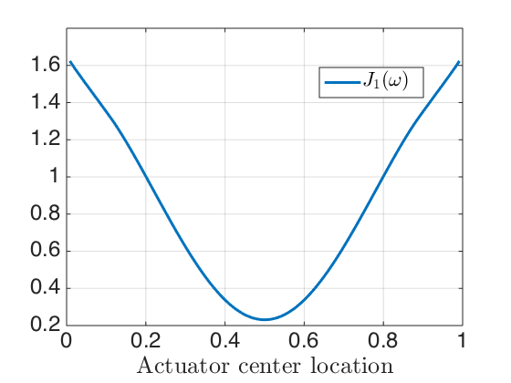
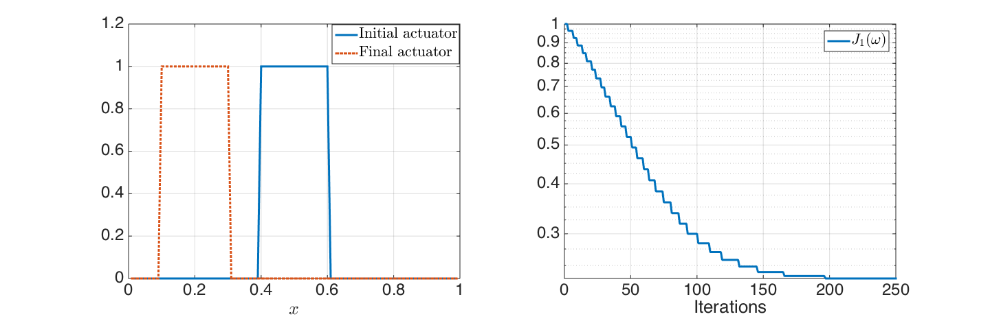
Figure 1: Test 1. Left: different single-component actuators with different centers have been spanned over the domain, locating the minimum value of $\mathcal{J}_{1}$ for the center at $x=0.5$. Center: starting from an initial guess for the actuator far from $0.5$, the gradient-based approach of Algorithm 1 locates the optimal position in the middle. Right: as the actuator moves towards the center in the subsequent iterations of Algorithm 1, the value $\mathcal{J}_{1}$ decays until reaching a stationary point.

Test 2

We consider the same setting as in the previous test, but we change the initial condition of the dynamics to be $y_{0}(x)=100|x-0.7|^{4}+x(x-1)$, so the setting is asymmetric and the optimal position is different from the center. Results are shown in Figure 2, where the numerical solution coincides with the result obtained by inspecting all the possible locations.

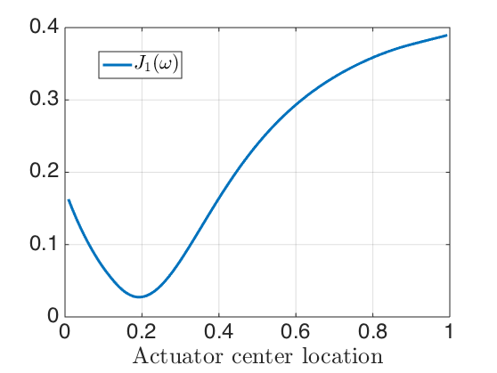
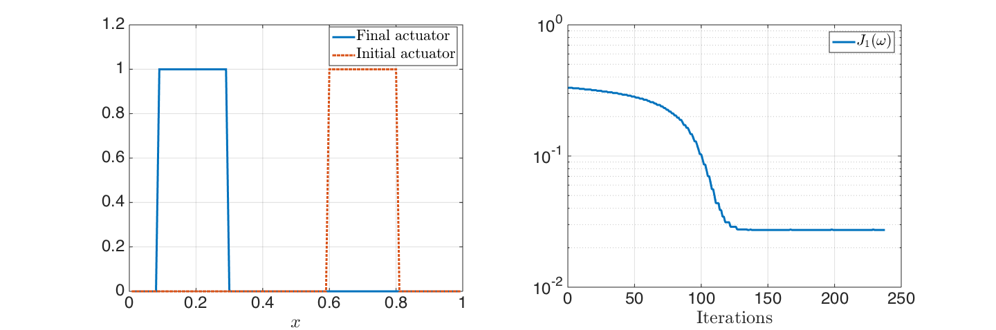
Figure 2: Test 2. Left: inspecting different values of $\mathcal{J}_{1}$ by spanning actuators with different centers, the optimal center location is found to be close to $0.2$ . Center: the gradient-based approach steers the initial actuator to the optimal position. Right: the value $\mathcal{J}_{1}$ decays until reaching a stationary point, which coincides with the minimum for the first plot on the left.

6.2 Optimal actuator design through topological derivatives

In the following series of experiments we focus on 1D optimal actuator design, i.e. problems (9) and (10) without any further parametrisation of the actuator, thus allowing multi-component structures. For this, we consider the approach combining the topological derivative, with a level-set method, as summarized in Algorithm 2.

Test 3

For $y_{0}(x)=\max(\sin(3\pi x),0)^{2}$, results are presented in Figures 3 and 4 . As it can be expected from the symmetry of the problem, and from the initial condition, the actuator splits into two equally sized components. We carried out two types of tests, one without and one with a continuation strategy with respect to $\alpha$. Without a continuation strategy, choosing $\alpha=10^{3}$ we obtain the result depicted in Figure 3 (b). With a continuation strategy, as the penalty increases, the size of the components decreases until approaching the total size constraint. The behavior of this continuation approach is shown in Table 1. When $\alpha$ is increased, the size of the actuator tends to $0.2$, the reference size, while the LQ part of $\mathcal{J}_{1}$, tends to a stationary value. For a final value of $\alpha=10^{4}$, the overall cost $\mathcal{J}_{1}$ obtained via the continuation approach is approx. 80 times smaller than the value obtained without any initialisation procedure, see Figure 3 (b)-(d). Figure 4 illustrates some basic relevant aspects of the level-set approach, such as the update of the shape (left), the computation of the level-set update upon $\beta_{n}$ and $\psi_{h}^{n}$ (middle), and the decay of the value $J_{1}$ (right).

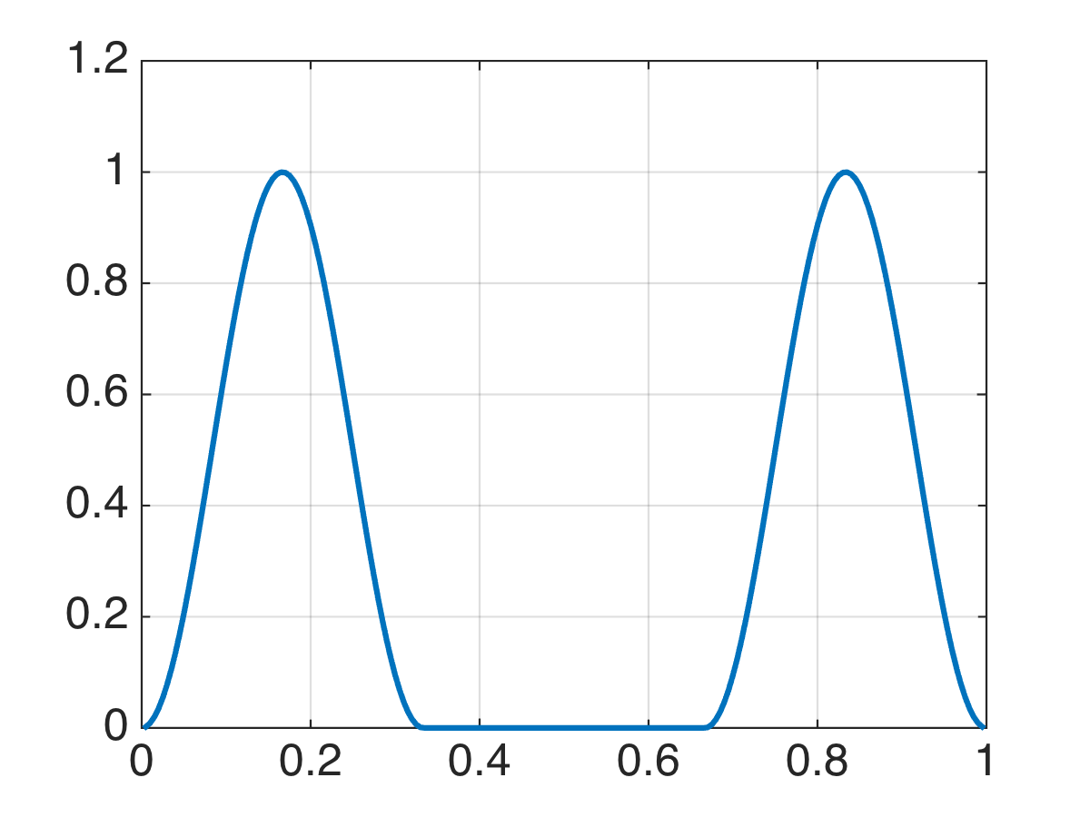
(a) $y_{0}(x)$

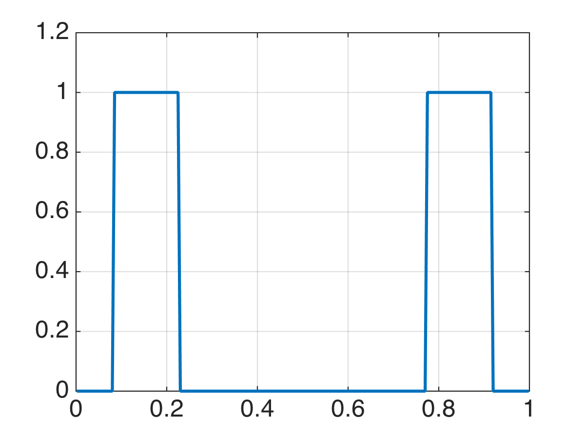
(b) $\alpha=10^{3}$, no init.

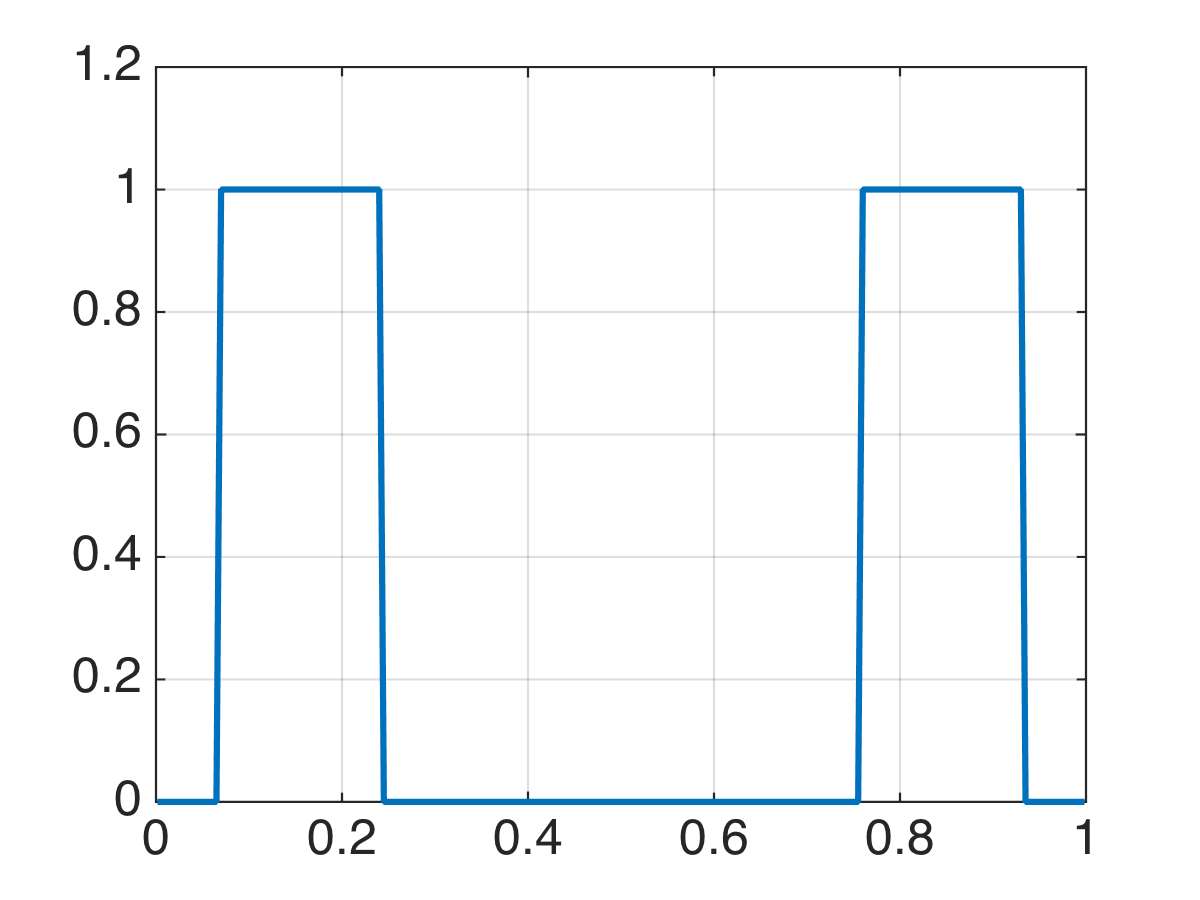
(c) $\alpha=10^{-1}$

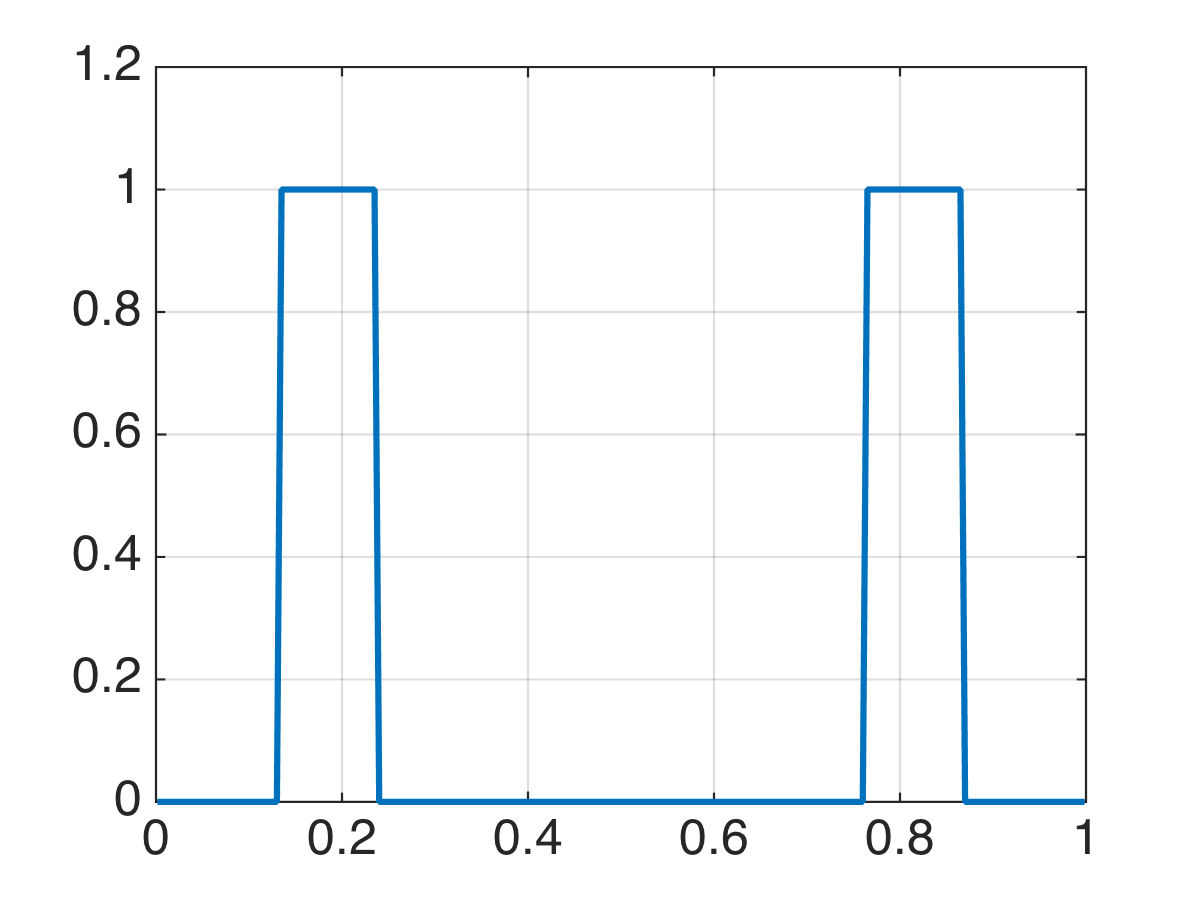
(d) $\alpha=10^{3}$

Figure 3: Test 3. (a) Initial condition $y_{0}(x)=\max(\sin(3\pi x),0)^{2}$. (b) Optimal actuator for $\alpha=10^{3}$, without initialization via increasing penalization. (c) Optimal actuator for $\alpha=10^{-1}$, subsequently used in the quadratic penalty approach. (d) Optimal actuator for $\alpha=10^{3}$, via increasing penalization.

$\alpha$	$\mathcal{J}_{1}$	$\mathcal{J}_{1}^{LQ}$	$\mathcal{J}_{1}^{\alpha}(size)$	iterations
0.1	1.84$\times 10^{-2}$	1.62$\times 10^{-2}$	2.30$\times 10^{-3}$ (0.35)	225
1	2.35$\times 10^{-2}$	2.26$\times 10^{-2}$	9.10$\times 10^{-4}$ (0.23)	226
10	2.56$\times 10^{-2}$	2.46$\times 10^{-2}$	1.00$\times 10^{-3}$ (0.21)	316
$10^{2}$	3.46$\times 10^{-2}$	2.46$\times 10^{-2}$	1.00$\times 10^{-2}$ (0.21)	226
$10^{3}$	0.12	2.46$\times 10^{-2}$	1.00$\times 10^{-1}$ (0.21)	226
$10^{3}$*	8.18	8.00$\times 10^{-2}$	8.10 (0.29)	629

Table 1: Test 3. optimisation values for $y_{0}(x)=\max(\sin(3\pi x),0)^{2}$. Each row is initialized with the optimal actuator corresponding to the previous one, except for the last row with $\alpha=10^{3}*$, illustrating that incorrectly initialized solves lead to suboptimal solutions. The reference size for the actuator is $0.2$ .

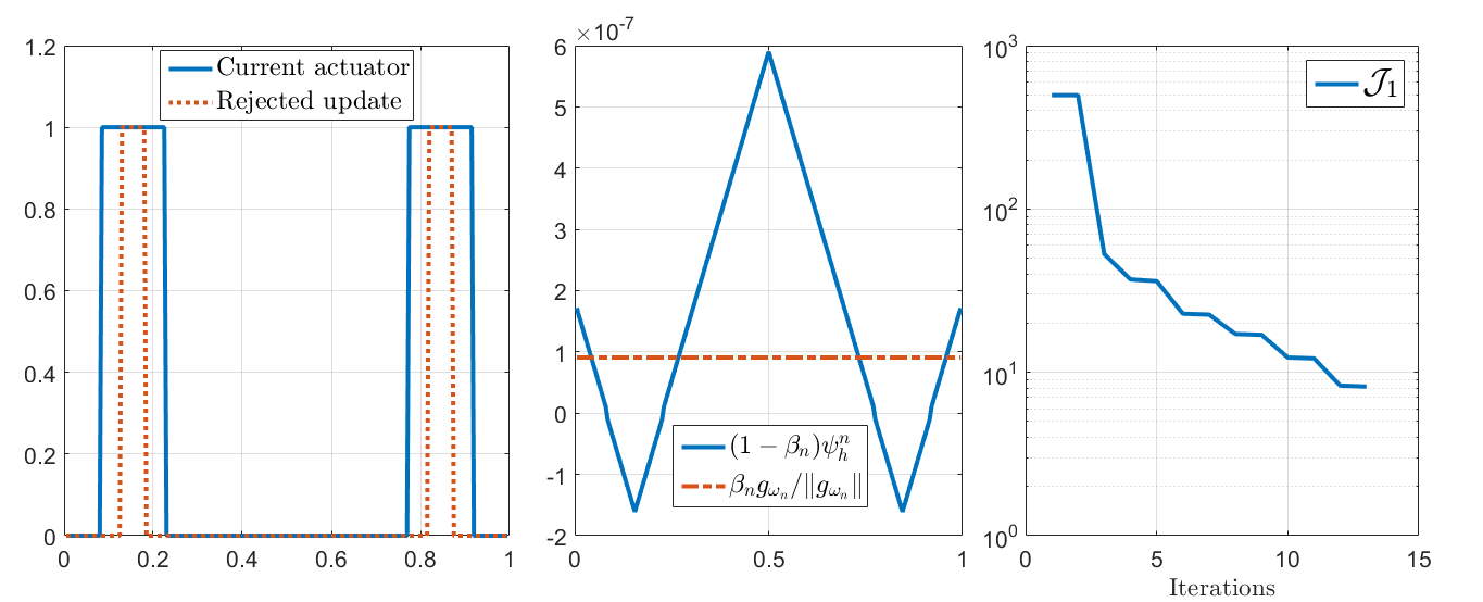
Figure 4: Test 3. Level set method implemented in Algorithm 2. Left: starting from an initial actuator, the topological derivative of the cost is computed and an updated actuator is obtained. The new shape is evaluated according to its closed-loop performance. If the update is rejected, the parameter $\beta_{n}$ is reduced. Middle: the level-set approach generates an update of the actuator shape based on the information from $\psi_{h}^{n}$, $\beta_{n}$ and $g_{\omega_{n}}$. Right: This iterative loop generates a decay in the total cost $J_{1}$, (which accounts for both the closed-loop performance of the actuator and its volume constraint).

Test 4

We repeat the setting of Test 3 with a nonsymmetric initial condition $y_{0}(x)=\sin(3\pi x)^{2}\chi_{\{x<2/3\}}(x)$. Results are presented in Table 2 and Figure 5, which illustrate the effectivity of the continuation approach, which generates an optimal actuator with two components of different size, see Figure 5d and compare with Figure 5b.

$\alpha$	$\mathcal{J}_{1}$	$\mathcal{J}_{1}^{LQ}$	$\mathcal{J}_{1}^{\alpha}(size)$	iterations
0.1	6.48$\times 10^{-2}$	6.31$\times 10^{-2}$	1.7$\times 10^{-3}$ (0.33)	229
1	8.0$\times 10^{-2}$	6.31$\times 10^{-2}$	1.69-2 (0.33)	226
10	0.176	0.164	1.23$\times 10^{-2}$ (0.235)	226
$10^{2}$	0.207	0.184	2.25$\times 10^{-2}$ (0.215)	316
$10^{3}$	0.234	0.209	2.50$\times 10^{-2}$ (0.195)	316
$10^{4}$	0.459	0.209	0.250 (0.195)	316
$10^{4}$*	9.09	9.66$\times 10^{-2}$	9 (0.23)	629

Table 2: Test 4. optimisation values for $y_{0}(x)=\sin(3\pi x)^{2}\chi_{x<2/3}(x)$. Each row is initialized with the optimal actuator corresponding to the previous one, except for the last row with $\alpha=10^{4}*$, illustrating that incorrectly initialized solves lead to suboptimal solutions. The reference size for the actuator is $0.2$ .

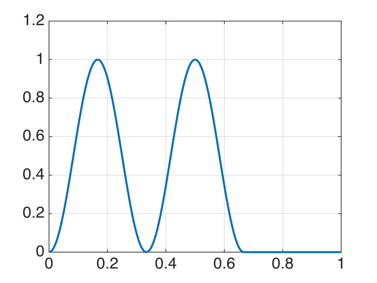
(a) $y_{0}(x)$

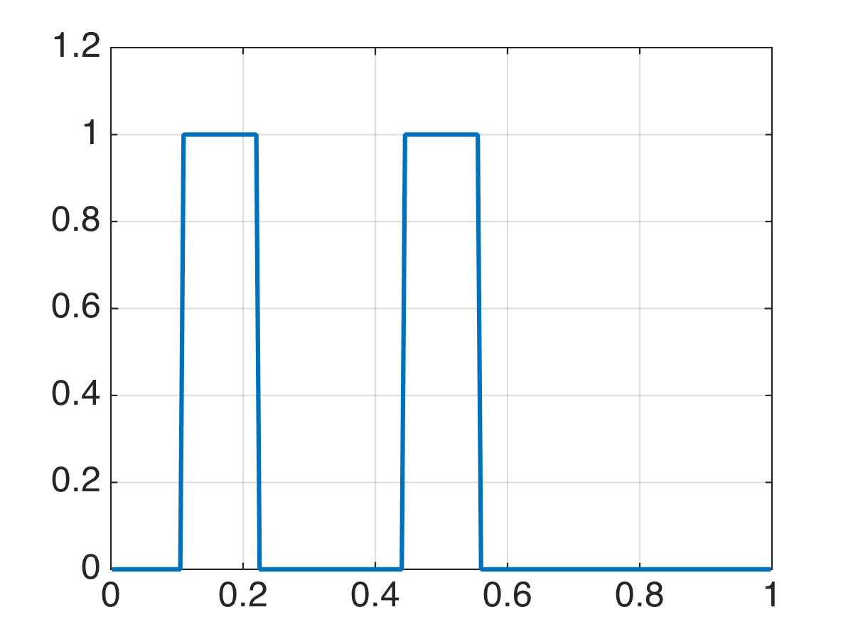
(b) $\alpha=10^{4}$, no init.

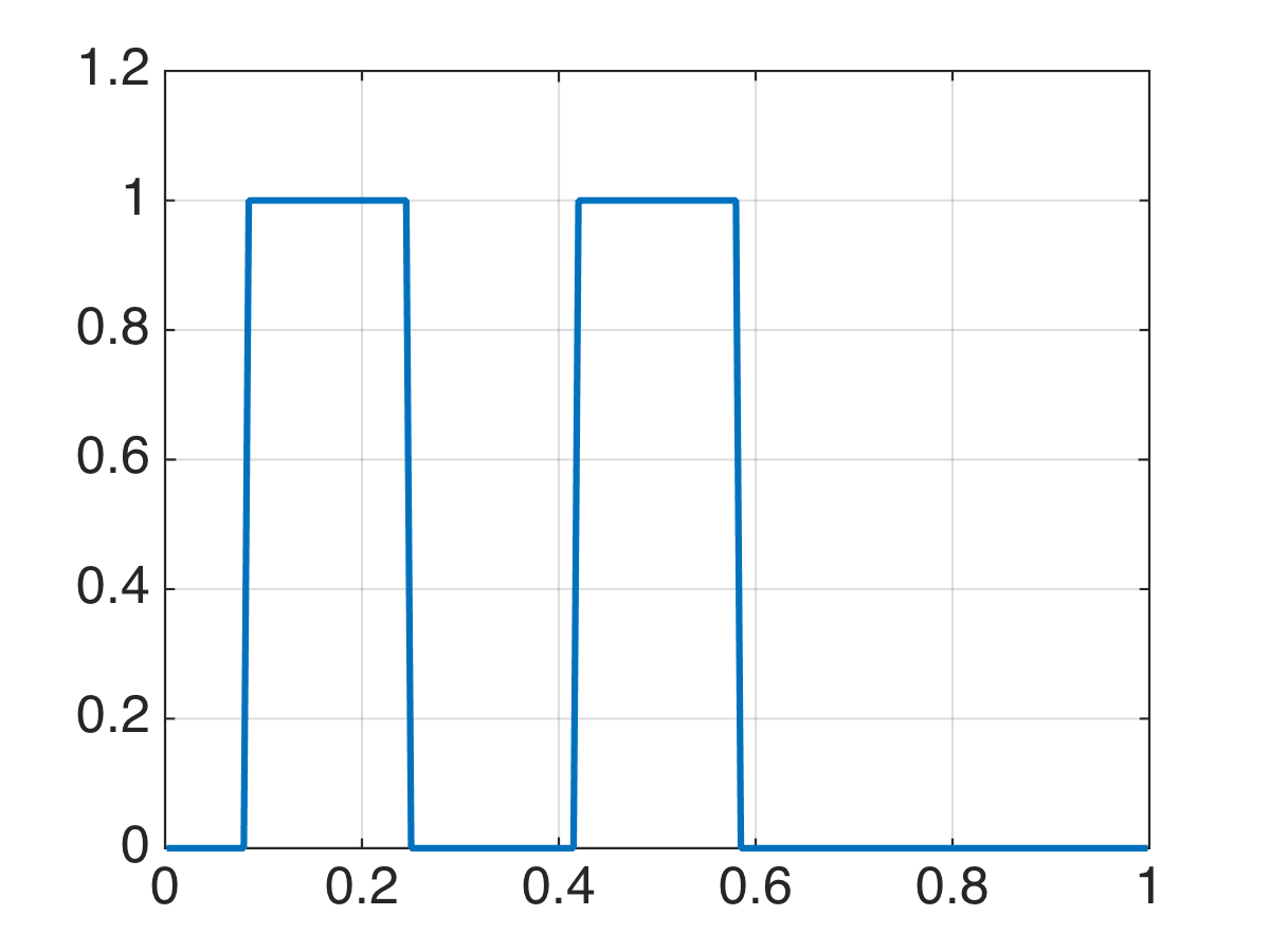
(c) $\alpha=10^{-1}$

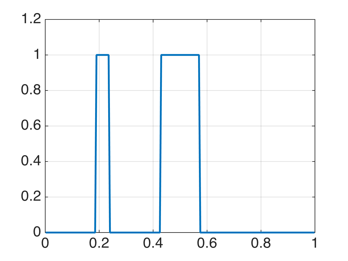
(d) $\alpha=10^{4}$

Figure 5: Test 4. (a) Initial condition $y_{0}(x)=\sin(3\pi x)^{2}\chi_{\{x<2/3\}}(x)$. (b) Optimal actuator for $\alpha=10^{4}$, without initialization via increasing penalization. (c) Optimal actuator for $\alpha=10^{-1}$, subsequently used in the quadratic penalty approach. (d) Optimal actuator for $\alpha=10^{4}$, via increasing penalization.

Test 5

We now turn our attention to the optimal actuator design for the worst-case scenario among all the initial conditions, i.e. the $\mathcal{J}_{2}$ setting. Results are presented in Figure 6 and Table 3. The worst-case scenario corresponds to the first eigenmode of the Riccati operator (Figure 6a), which generates a two-component symmetric actuator (Figure 6d). This is only observed within the continuation approach. For a large value of $\alpha$ without initialisation, we obtain a suboptimal solution with a single component (last row of Table 3, Figure 6b).

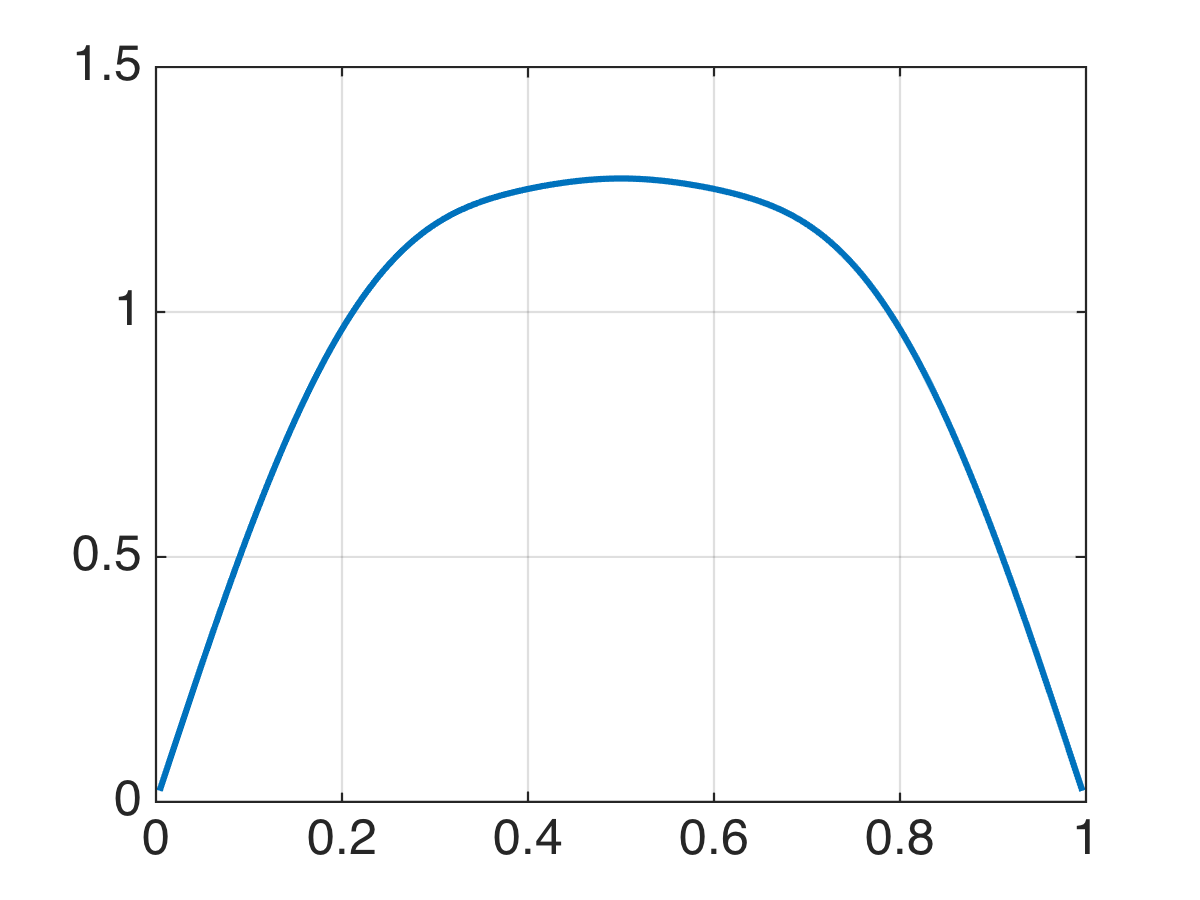
(a) $\mathfrak{X}_{2}(\omega)$

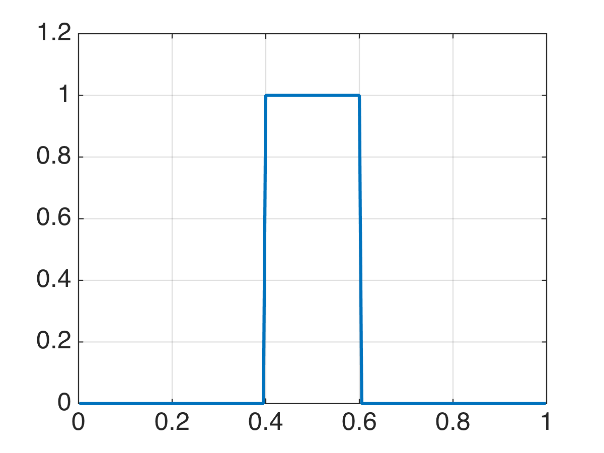
(b) $\alpha=10^{3}$, no init.

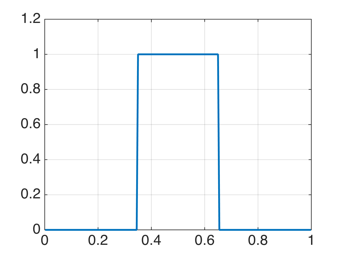
(c) $\alpha=10^{-1}$

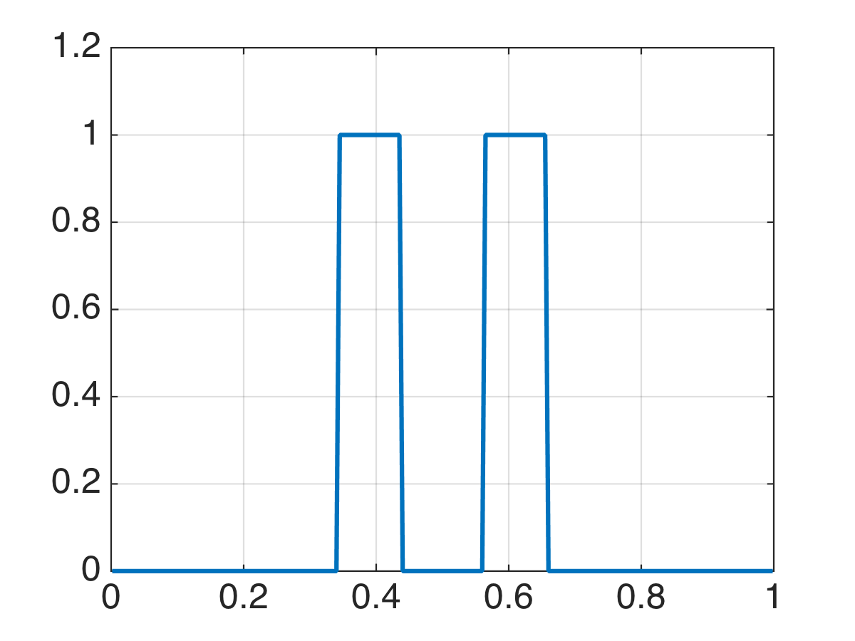
(d) $\alpha=10^{3}$

Figure 6: Test 5. (a) First eigenmode of the Riccati operator, which corresponds to the set $\mathfrak{X}_{2}(\omega)$. (b) Optimal actuator for $\alpha=10^{3}$, without initialization via increasing penalization. (c) Optimal actuator for $\alpha=10^{-1}$, subsequently used in the quadratic penalty approach. (d) Optimal actuator for $\alpha=10^{3}$, via increasing penalization.

$\alpha$	$\mathcal{J}_{2}$	$\mathcal{J}_{2}^{LQ}$	$\mathcal{J}_{2}^{\alpha}(size)$	iterations
0.1	0.402	0.401	1.1$\times 10^{-3}$ (0.305)	307
1	0.369	0.364	4.0$\times 10^{-4}$ (0.22)	225
10	0.343	0.342	1.0$\times 10^{-3}$ (0.19)	228
$10^{2}$	0.352	0.342	1.0$\times 10^{-2}$ (0.19)	226
$10^{3}$	0.442	0.342	0.1 (0.19)	226
$10^{3}$*	0.761	0.536	0.225 (0.215)	941

Table 3: Test 5. optimisation values for $\mathcal{J}_{2}$. Each row is initialized with the optimal actuator corresponding to the previous one, except for the last row with $\alpha=10^{3}$*. The reference size for the actuator is $0.2$ .

Test 6

As an extension of the capabilities of the proposed approach, we explore the $\mathcal{J}_{2}$ setting with space-dependent diffusion. For this test, the diffusion operator $\sigma\Delta y$ is rewritten as $div(\sigma(x)\nabla y)$, with $\sigma(x)=(1-\max(\sin(9\pi x),0))\chi_{\{x<0.5\}}(x)+10^{-3}$. Iterates of the continuation approach are presented in Table 4. Again, the lack of a proper initialization of Algortithm 2 with a large value of $\alpha$ leads to a poor satisfaction of both the size constraint and the LQ performance, which is solved via the increasing penalty approach. A two-component actuator present in the area of smaller diffusion is observed in Figure 7d.

$\alpha$	$\mathcal{J}_{2}$	$\mathcal{J}_{2}^{LQ}$	$\mathcal{J}_{2}^{\alpha}(size)$	iterations
0.1	1.792	1.743	4.97$\times 10^{-2}$ (0.908)	194
1	2.240	1.743	0.497 (0.908)	228
10	4.734	4.462	0.272 (0.365)	225
$10^{2}$	3.134	3.071	6.25$\times 10^{-2}$ (0.175)	538
$10^{3}$	1.023	0.998	0.025 (0.195)	226
$10^{4}$	1.248	0.998	0.250 (0.195)	226
$10^{4}$*	28.19	3.195	25.0 (0.25)	673

Table 4: Test 6. $\mathcal{J}_{2}$ values with space-dependent diffusion $\sigma(x)=(1-\max(\sin(9\pi x),0))\chi_{\{x<0.5\}}(x)+10^{-3}$. Each row is initialized with the optimal actuator corresponding to the previous one, except for the last row with $\alpha=10^{4}$*. The reference size for the actuator is $0.2$ .

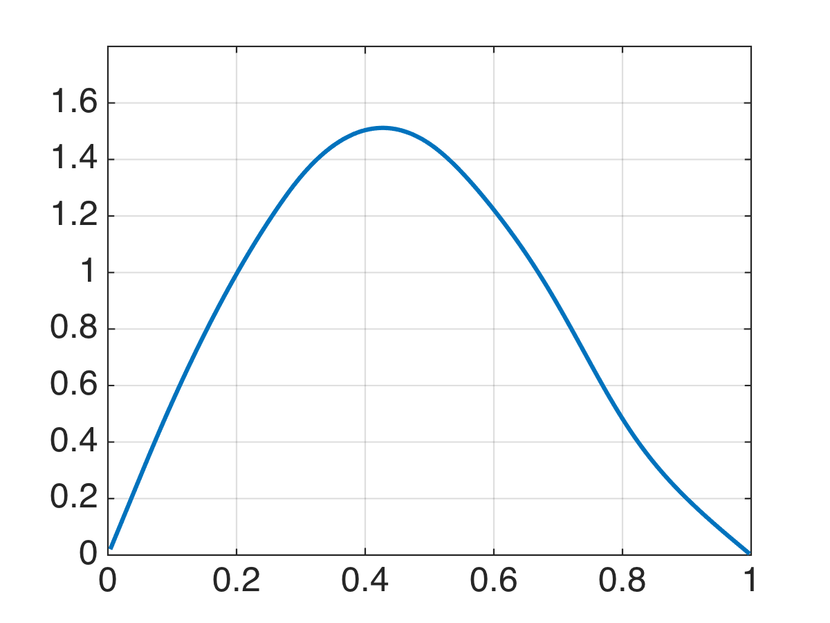
(a) $\mathfrak{X}_{2}(\omega)$

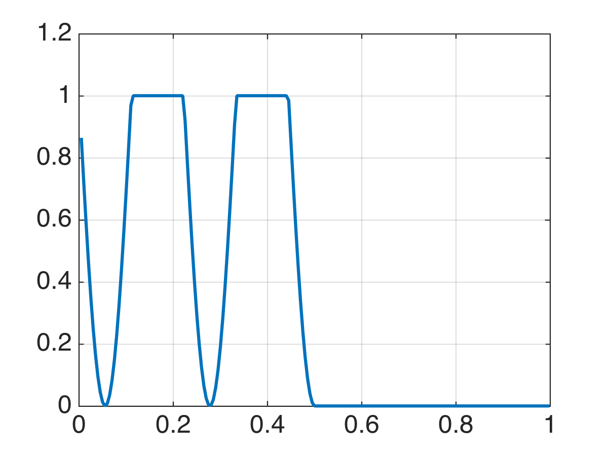
(b) $\sigma(x)$

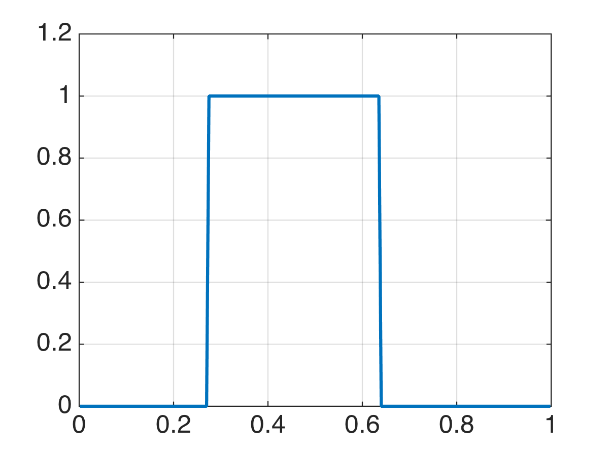
(c) $\alpha=0.1$

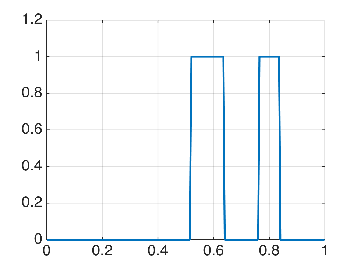
(d) $\alpha=10^{4}$

Figure 7: Test 6. (a) First eigenmode of the Riccati operator, which corresponds to the set $\mathfrak{X}_{2}(\omega)$. (b) space-dependent diffusion coefficient $\sigma(x)=(1-\max(\sin(9\pi x),0))\chi_{\{x<0.5\}}(x)+10^{-3}$. (c) Optimal actuator for $\alpha=10$, subsequently used in the quadratic penalty approach. (d) Optimal actuator for $\alpha=10^{4}$, via increasing penalization.

6.3 Two-dimensional optimal actuator design

We now turn our attention into assessing the performance of Algorithm 2 for two-dimensional actuator topology optimisation. While this problem is computationally demanding, the increase of degrees of freedom can be efficiently handled via modal expansions, as explained at the beginning of this Section. We explore both the $\mathcal{J}_{1}$ and $\mathcal{J}_{2}$ settings.

Test 7

This experiment is a direct extension of Test 3. We consider a unilaterally symmetric initial condition $y_{0}(x_{1},x_{2})=\max(\sin(4\pi(x_{1}-1/8)),0)^{3}\sin(\pi x_{2})^{3}$, inducing a two-component actuator. The desired actuator size is $c=0.04$. The evolution of the actuator design for increasing values of the penalty parameter $\alpha$ is depicted in Figure 8. We also study the closed-loop performance of the optimal shape. For this purpose the running cost associated to the optimal actuator is compared against an ad-hoc design, which consists of a cylindrical actuator of desired size placed in the center of the domain, see Figure 9 . The closed-loop dynamics of the optimal actuator generate a stronger exponential decay compared to the uncontrolled dynamics and the ad-hoc shape.

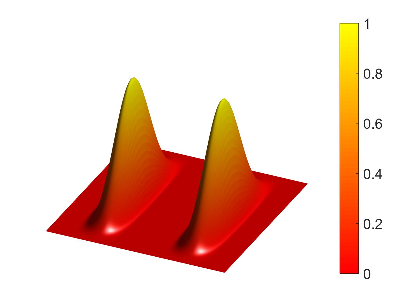
(a) $y_{0}(x_{1},x_{2})$

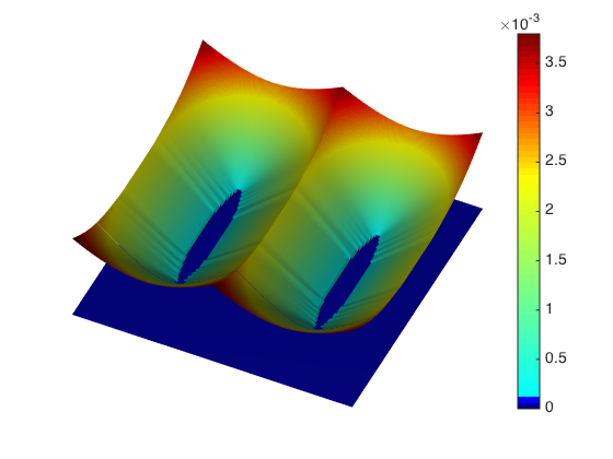
(b) $\psi_{h}^{n+1}$

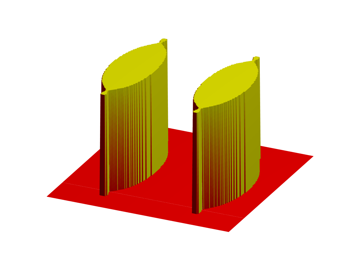
(c) $\alpha=0.1$

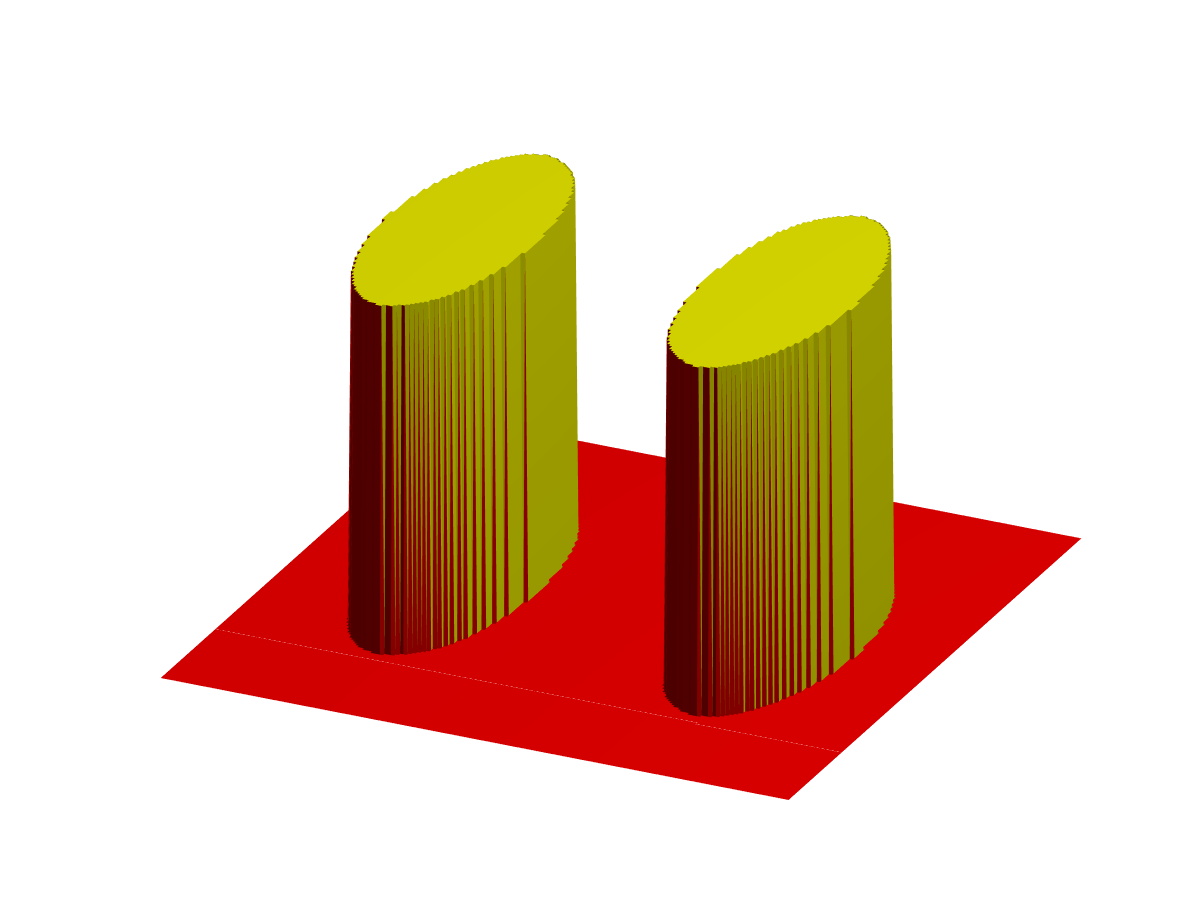
(d) $\alpha=1$

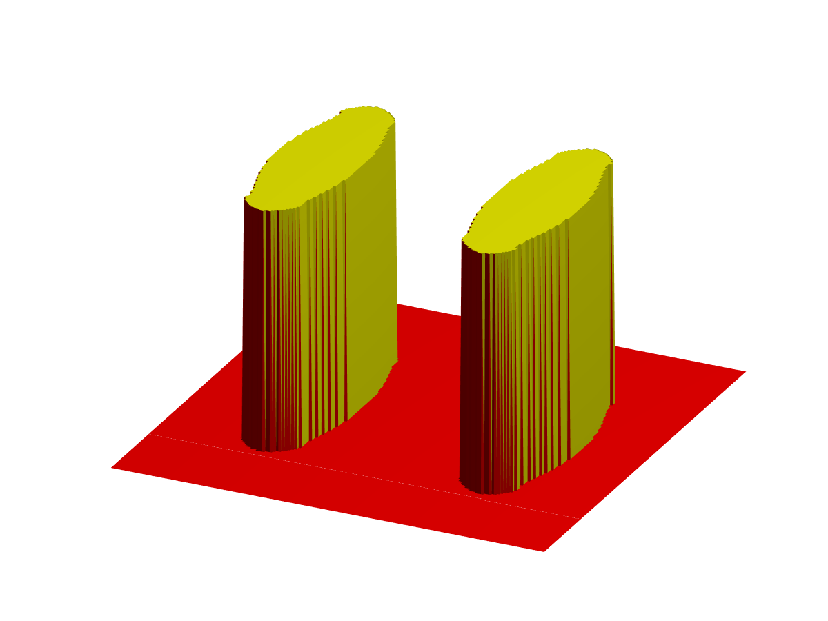
(e) $\alpha=1\times 10^{2}$

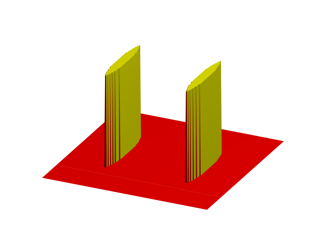
(f) $\alpha=10^{4}$

Figure 8: Test 7. (a) initial condition $y_{0}(x_{1},x_{2})=\max(\sin(4\pi(x_{1}-1/8)),0)^{3}\sin(\pi x_{2})^{3}$ for $\mathcal{J}_{1}$ optimisation. (b) within the level-set method, the actuator is updated according to the zero level-set of the function $\psi_{h}^{n+1}$. (c) to (f) optimal actuators for different volume penalties.

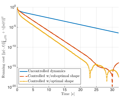
Figure 9: Test 7. Closed-loop performance for different shapes. The running cost in $\mathcal{J}_{1}$ is evaluated for uncontrolled dynamics ($u\equiv 0$), an ad-ho cylindrical actuator located in the center of the domain, and the optimal shape (Figure 8f). Closed-loop dynamics of the optimal shape decay faster.

Test 8

In an analogous way as in Test 5, we study the optimal design problem associated to $\mathcal{J}_{2}$. The first eigenmode of the Riccati operator is shown in Figure 10a. The increasing penalty approach (Figs. 10c to 10f) shows a complex structure, with a hollow cylinder and four external components. The performance of the closed-loop optimal solution is analysed in Figure 11, with a considerably faster decay compared to the uncontrolled solution, and to the ad-hoc design utilised in the previous test.

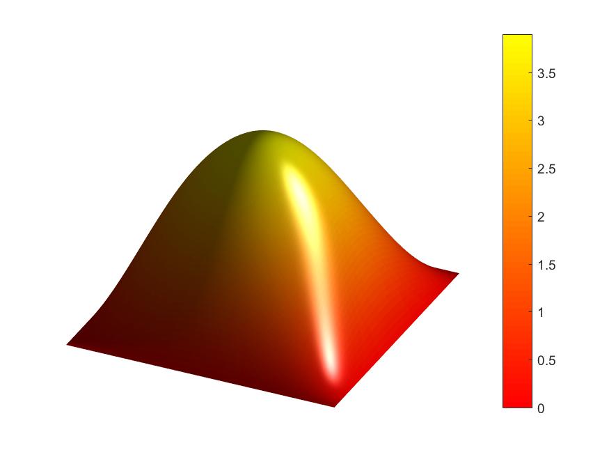
(a) $\mathfrak{X}_{2}(\omega)$

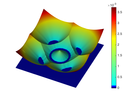
(b) $\psi_{h}^{n+1}$

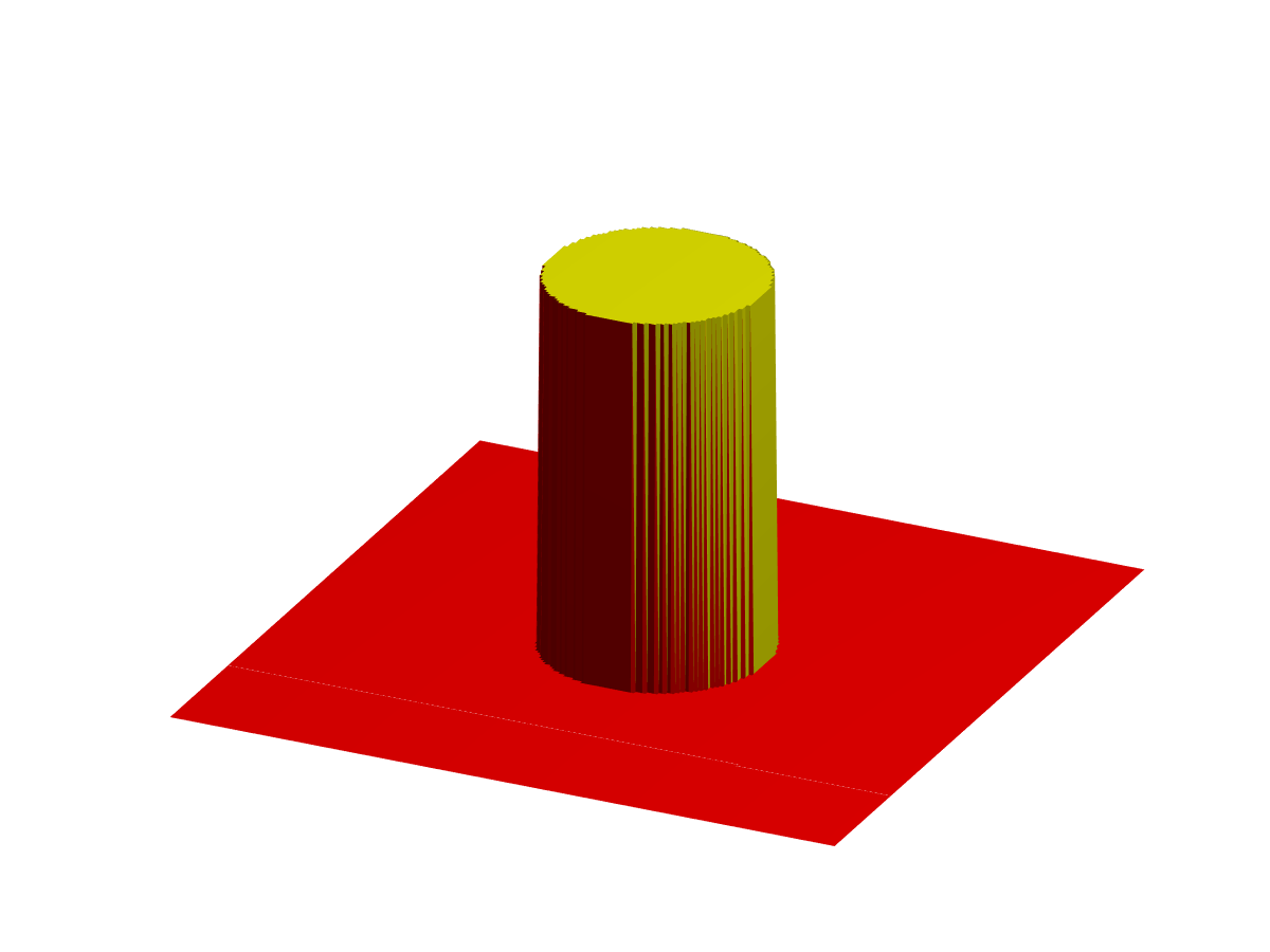
(c) $\alpha=0.1$

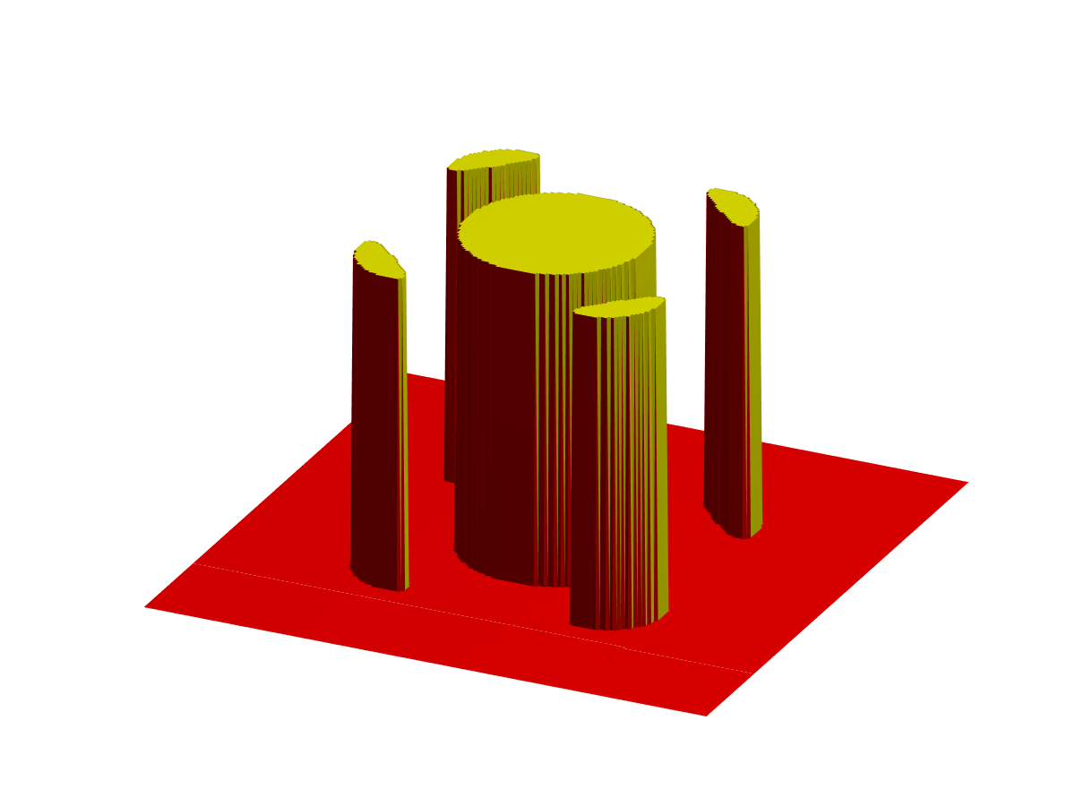
(d) $\alpha=10$

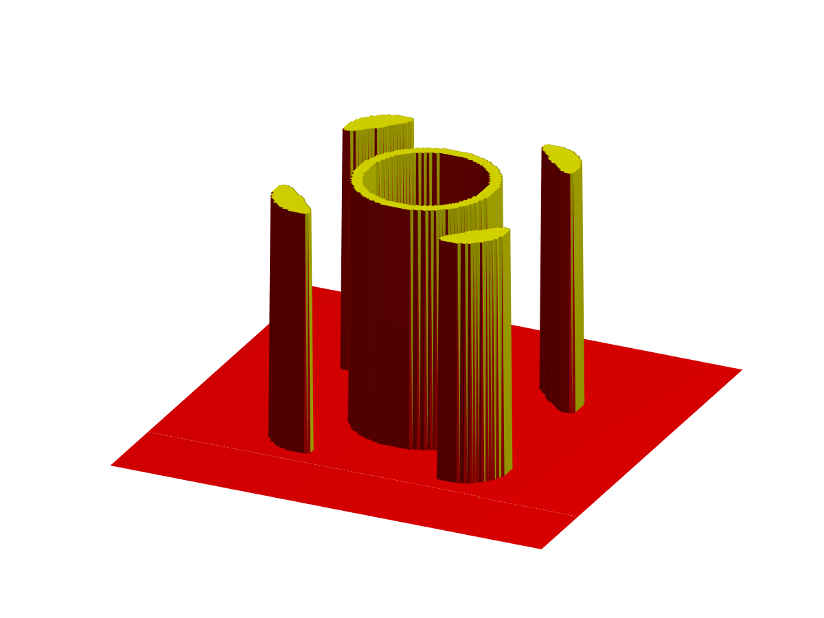
(e) $\alpha=10^{2}$

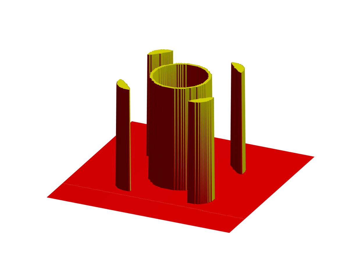
(f) $\alpha=10^{4}$

Figure 10: Test 8. (a) first eigenmode of the Riccati operator. (b) within the level-set method, the actuator is updated according to the zero level-set of the function $\psi_{h}^{n+1}$. (c) to (f) optimal actuators for different volume penalties.

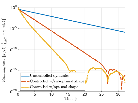
Figure 11: Test 8. Closed-loop performance for different shapes. The running cost in $\mathcal{J}_{2}$ is evaluated for uncontrolled dynamics ($u\equiv 0$), a suboptimal cylindrical actuator of size $c$ located in the center of the domain, and the optimal shape with five components (Figure 10f). Closed-loop dynamics of the optimal shape decay faster.

Concluding remarks

In this work we have developed an analytical and computational framework for optimisation-based actuator design. We derived shape and topological sensitivities formulas which account for the closed-loop performance of a linear-quadratic controller associated to the actuator configuration. We embedded the sensitivities into gradient-based and level-set methods to numerically realise the optimal actuators. Our findings seem to indicate that from a practical point of view, shape sensitivities are a good alternative whenever a certain parametrisation of the actuator is fixed in advance and only optimal position is sought. Topological sensitivities are instead suitable for optimal actuator design in a wider sense, allowing the emergence of nontrivial multi-component structures, which would be difficult to guess or parametrise a priori. This is a relevant fact, as most of the engineering literature associated to computational optimal actuator positioning is based on heuristic methods which strongly rely on experts’ knowledge and tuning. Extensions concerning robust control design and semilinear parabolic equation are in our research roadmap.

Appendix

Differentiability of maximum functions

In order to prove Lemma 3.27 we recall the following Danskin-type lemmas.

Let $\mathfrak{V}_{1}$ be a nonempty set and let $\mathcal{G}:[0,\tau]\times\mathfrak{V}_{1}\rightarrow\mathbf{R}$ be a function, $\tau>0$. Introduce the function $g_{1}:[0,\tau]\rightarrow\mathbf{R}$,

(166) $$g_{1}(t):=\sup_{x\in\mathfrak{V}_{1}}\mathcal{G}(t,x),$$

and let $\ell:[0,\tau]\rightarrow\mathbf{R}$ be any function such that $\ell(t)>0$ for $t\in(0,\tau]$ and $\ell(0)=0$. We give sufficient conditions that guarantee that the limit

(167) $$\frac{d}{d\ell}g_{1}(0^{+}):=\lim_{t\searrow 0}\frac{g_{1}(t)-g_{1}(0)}{\ell(t)}$$

exists. For this purpose we introduce for each $t$ the set of maximisers

(168) $$\mathfrak{V}_{1}(t)=\{x^{t}\in\mathfrak{V}_{1}:\;\sup_{x\in\mathfrak{V}_{1}}\mathcal{G}(t,x)=\mathcal{G}(t,x^{t})\}.$$

The next lemma can be found with slight modifications in [7, Theorem 2.1, p. 524].

Lemma 6.1.

Let the following hypotheses be satisfied.

• • For all $t$ in $[0,\tau]$ the set $\mathfrak{V}_{1}(t)$ is nonempty,

  • the limit

    (169) $$\partial_{\ell}\mathcal{G}(0^{+},x):=\lim_{t\searrow 0}\frac{\mathcal{G}(t,x)-\mathcal{G}(0,x)}{\ell(t)}$$

    exists for all $x\in\mathfrak{V}_{1}(0)$.

• For all real null-sequences $(t_{n})$ in $(0,\tau]$ and all sequence $(x_{t_{n}})$ in $\mathfrak{V}_{1}(t_{n})$, there exists a subsequence $(t_{n_{k}})$ of $(t_{n})$, $(x_{t_{n_{k}}})$ in $\mathfrak{V}_{1}(t_{n_{k}})$ and $x_{0}$ in $\mathfrak{V}_{1}(0)$, such that

  (170) $$\lim_{k\rightarrow\infty}\frac{\mathcal{G}(t_{n_{k}},x_{t_{n_{k}}})-\mathcal{G}(0,x_{t_{n_{k}}})}{\ell(t_{n_{k}})}=\partial_{\ell}\mathcal{G}(0^{+},x_{0}).$$

Then $g_{1}$ is differentiable at $t=0^{+}$ with derivative

(171) $$\frac{d}{dt}g_{1}(t)|_{t=0^{+}}=\max_{x\in\mathfrak{V}_{1}(0)}\partial_{\ell}\mathcal{G}(0^{+},x).$$

Proof of Lemma 3.27

Our strategy is to prove Lemma 3.27 by applying
Lemma 6.1 to the function $\mathcal{G}(t,y):=\inf_{x\in\mathfrak{V}}G(t,x,y)$ with $\mathfrak{V}_{1}:=\mathfrak{V}$. This will show that $g(t):=\sup_{y\in\mathfrak{V}}\mathcal{G}(t,y)$ is right-differentiable at $t=0^{+}$. By construction Assumption (A0) of Lemma 3.27 is satisfied.

Step 1: For every $t\in[0,\tau]$ and $y\in\mathfrak{V}$ we have $\mathcal{G}(t,y)=G(t,x^{t,y},y)$. Hence

(172) $$\begin{split}\mathcal{G}(t,y)-\mathcal{G}(0,y)=&G(t,x^{t,y},y)-G(0,x^{0,y},y)\\ &=G(t,x^{t,y},y)-G(0,x^{t,y},y)+\underbrace{G(0,x^{t,y},y)-G(0,x^{0,y},y)}_{\geq 0}\\ &\geq G(t,x^{t,y},y)-G(0,x^{t,y},y)\end{split}$$

and similarly

(173) $$\begin{split}\mathcal{G}(t,y)-\mathcal{G}(0,y)=&G(t,x^{t,y},y)-G(0,x^{0,y},y)\\ &=\underbrace{G(t,x^{t,y},y)-G(t,x^{0,y},y)}_{\leq 0}+G(t,x^{0,y},y)-G(0,x^{0,y},y)\\ &\leq G(t,x^{0,y},y)-G(0,x^{0,y},y).\end{split}$$

Therefore using Assumption (A2) of Lemma 3.27 we obtain from (99) and (100)

(174) $$\liminf_{t\searrow 0}\frac{\mathcal{G}(t,y)-\mathcal{G}(0,y)}{\ell(t)}\geq\partial_{\ell}G(0^{+},x^{0,y},y)\geq\limsup_{t\searrow 0}\frac{\mathcal{G}(t,y)-\mathcal{G}(0,y)}{\ell(t)}.$$

Hence Assumption (A1) of Lemma 6.1 is satisfied.

Step 2: For every $t\in[0,\tau]$ and $y^{t}\in\mathfrak{V}(t)$ we have $\mathcal{G}(t,y^{t})=G(t,x^{t,y^{t}},y^{t})$ and hence

(175) $$\begin{split}\mathcal{G}(t,y^{t})-\mathcal{G}(0,y^{t})=&G(t,x^{t,y^{t}},y^{t})-G(0,x^{0,y^{t}},y^{t})\\ =&G(t,x^{t,y^{t}},y^{t})-G(0,x^{t,y^{t}},y^{t})+\underbrace{G(0,x^{t,y^{t}},y^{t})-G(0,x^{0,y^{t}},y^{t})}_{\geq 0}\\ \geq&G(t,x^{t,y^{t}},y^{t})-G(0,x^{t,y^{t}},y^{t})\end{split}$$

and similarly

(176) $$\begin{split}\mathcal{G}(t,y^{t})-\mathcal{G}(0,y^{t})=&\underbrace{G(t,x^{t,y^{t}},y^{t})-G(t,x^{0,y^{t}},y^{t})}_{\leq 0}+G(t,x^{0,y^{t}},y^{t})-G(0,x^{0,y^{t}},y^{t})\\ \leq&G(t,x^{0,y^{t}},y^{t})-G(0,x^{0,y^{t}},y^{t}).\end{split}$$

Thanks to Assumption (A3) of Lemma 3.27 For all real null-sequences $(t_{n})$ in $(0,\tau]$ and all sequences $(y^{t_{n}})$, $y^{t_{n}}\in\mathfrak{V}(t_{n})$, there exists a subsequence $(t_{n_{k}})$ of $(t_{n})$, $(y^{t_{n_{k}}})$ of $(y^{t_{n}})$, and $y^{0}$ in $\mathfrak{V}(0)$, such that

(177) $$\lim_{k\rightarrow\infty}\frac{G(t_{n_{k}},x^{t_{n_{k}},y^{t_{n_{k}}}},y^{t_{n_{k}}})-G(0,x^{t_{n_{k}},y^{t_{n_{k}}}},y^{t_{n_{k}}})}{\ell(t_{n_{k}})}=\partial_{\ell}G(0^{+},x^{0,y^{0}},y^{0})$$

and

(178) $$\lim_{k\rightarrow\infty}\frac{G(t_{n_{k}},x^{0,y^{t_{n_{k}}}},y^{t_{n_{k}}})-G(0,x^{0,y^{t_{n_{k}}}},y^{t_{n_{k}}})}{\ell(t_{n_{k}})}=\partial_{\ell}G(0^{+},x^{0,y^{0}},y^{0}).$$

Hence choosing $t=t_{n_{k}}$ in (175) we obtain

(179) $$\begin{split}&\liminf_{k\to\infty}\frac{\mathcal{G}(t_{n_{k}},y^{t_{n_{k}}})-\mathcal{G}(0,y^{t_{n_{k}}})}{\ell(t_{n_{k}})}\\ &\stackrel{{\scriptstyle\eqref{eq:difference_ge}}}{{\geq}}\liminf_{k\rightarrow\infty}\frac{G(t_{n_{k}},x^{t_{n_{k}},y^{t_{n_{k}}}},y^{t_{n_{k}}})-G(0,x^{t_{n_{k}},y^{t_{n_{k}}}},y^{t_{n_{k}}})}{\ell(t_{n_{k}})}\\ &\stackrel{{\scriptstyle\eqref{eq:limit1}}}{{=}}\partial_{\ell}G(0^{+},x^{0,y^{0}},y^{0})\end{split}$$

and similarly choosing $t=t_{n_{k}}$ in (176) we get

(180) $$\begin{split}&\limsup_{k\to\infty}\frac{\mathcal{G}(t_{n_{k}},y^{t_{n_{k}}})-\mathcal{G}(0,y^{t_{n_{k}}})}{\ell(t_{n_{k}})}\\ &\stackrel{{\scriptstyle\eqref{eq:difference_le}}}{{\leq}}\limsup_{k\rightarrow\infty}\frac{G(t_{n_{k}},x^{0,y^{t_{n_{k}}}},y^{t_{n_{k}}})-G(0,x^{0,y^{t_{n_{k}}}},y^{t_{n_{k}}})}{\ell(t_{n_{k}})}\\ &\stackrel{{\scriptstyle\eqref{eq:limit2}}}{{=}}\partial_{\ell}G(0^{+},x^{0,y^{0}},y^{0}).\end{split}$$

Combining (179) and (180) we conclude that

(181) $$\lim_{k\to\infty}\frac{\mathcal{G}(t_{n_{k}},y^{t_{n_{k}}})-\mathcal{G}(0,y^{t_{n_{k}}})}{\ell(t_{n_{k}})}=\partial_{\ell}G(0^{+},x^{0,y^{0}},y^{0}),$$

which is precisely Assumption (A2) of Lemma 6.1.

Step 1 and Step 2 together show that Assumptions (A1) and (A2) of Lemma 6.1 are satisfied and this finishes the proof.

References

- [1] A. Alla, M. Falcone, and D. Kalise, An efficient policy iteration algorithm for the solution of dynamic programming equations, SIAM J. Sci. Comput., 35 (2015), pp. A181–A200.
- [2] G. Allaire, F. Jouve, and A.-M. Toader, Structural optimization using sensitivity analysis and a level-set method, J. Comput. Phys., 194 (2004), pp. 363–393.
- [3] S. Amstutz, Augmented Lagrangian for cone constrained topology optimization, Comput. Optim. Appl., 49 (2011), pp. 101–122, https://doi.org/10.1007/s10589-009-9272-3, http://dx.doi.org/10.1007/s10589-009-9272-3.
- [4] S. Amstutz and H. Andrä, A new algorithm for topology optimization using a level-set method, J. Comput. Phys., 216 (2006), pp. 573–588, https://doi.org/10.1016/j.jcp.2005.12.015, http://dx.doi.org/10.1016/j.jcp.2005.12.015.
- [5] A. Bensoussan, Optimization of sensors’ location in a distributed filtering problem, Springer Berlin Heidelberg, Berlin, Heidelberg, 1972, pp. 62–84, https://doi.org/10.1007/BFb0064935, https://doi.org/10.1007/BFb0064935.
- [6] M. C. Delfour and J.-P. Zolésio, Shape sensitivity analysis via min max differentiability, SIAM J. Control Optim., 26 (1988), pp. 834–862, https://doi.org/10.1137/0326048, http://dx.doi.org/10.1137/0326048.
- [7] M. C. Delfour and J.-P. Zolésio, Shapes and geometries: Metrics, analysis, differential calculus, and optimization, Society for Industrial and Applied Mathematics (SIAM), Philadelphia, PA, second ed., 2011.
- [8] V. F. Dem′yanov and V. N. Malozëmov, Einführung in Minimax-Problem, Akademische Verlagsgesellschaft Geest & Portig K.-G., 1975. German translation.
- [9] A. El Jaïand A. J. Pritchard, Sensors and controls in the analysis of distributed systems, Ellis Horwood Series: Mathematics and its Applications, Ellis Horwood Ltd., Chichester; Halsted Press [John Wiley & Sons, Inc.], New York, 1988. Translated from the French by Catrin Pritchard and Rhian Pritchard.
- [10] L. C. Evans, Partial differential equations, vol. 19 of Graduate Studies in Mathematics, American Mathematical Society, Providence, RI, 1998.
- [11] F. Fahroo and M. A. Demetriou, Optimal actuator/sensor location for active noise regulator and tracking control problems, J. Comput. Appl. Math., 114 (2000), pp. 137–158, https://doi.org/10.1016/S0377-0427(99)00293-9, http://dx.doi.org/10.1016/S0377-0427(99)00293-9. Control of partial differential equations (Jacksonville, FL, 1998).
- [12] M. I. Frecker, Recent advances in optimization of smart structures and actuators, Journal of Intelligent Material Systems and Structures, 14 (2003), pp. 207–216, https://doi.org/10.1177/1045389X03031062, http://dx.doi.org/10.1177/1045389X03031062, https://arxiv.org/abs/http://dx.doi.org/10.1177/1045389X03031062.
- [13] P. Hébrard and A. Henrot, A spillover phenomenon in the optimal location of actuators, SIAM J. Control Optim., 44 (2005), pp. 349–366, https://doi.org/10.1137/S0363012903436247, http://dx.doi.org/10.1137/S0363012903436247.
- [14] M. Hintermüller, C. N. Rautenberg, M. Mohammadi, and M. Kanitsar, Optimal sensor placement: a robust approach, WIAS preprint, (2016), p. 34 pp., http://www.wias-berlin.de/preprint/2287/wias_preprints_2287.pdf.
- [15] K. Ito, K. Kunisch, and G. H. Peichl, Variational approach to shape derivatives, ESAIM Control Optim. Calc. Var., 14 (2008), pp. 517–539, https://doi.org/10.1051/cocv:2008002, http://dx.doi.org/10.1051/cocv:2008002.
- [16] D. Kasinathan and K. Morris, -optimal actuator location, IEEE Trans. Automat. Control, 58 (2013), pp. 2522–2535, https://doi.org/10.1109/TAC.2013.2266870, http://dx.doi.org/10.1109/TAC.2013.2266870.
- [17] Laurain, A. and Sturm, K., Distributed shape derivative via averaged adjoint method and applications, ESAIM: M2AN, 50 (2016), pp. 1241–1267.
- [18] K. Morris, Linear-quadratic optimal actuator location, IEEE Trans. Automat. Control, 56 (2011), pp. 113–124, https://doi.org/10.1109/TAC.2010.2052151, http://dx.doi.org/10.1109/TAC.2010.2052151.
- [19] K. Morris, M. A. Demetriou, and S. D. Yang, Using -control performance metrics for the optimal actuator location of distributed parameter systems, IEEE Trans. Automat. Control, 60 (2015), pp. 450–462, https://doi.org/10.1109/TAC.2014.2346676, http://dx.doi.org/10.1109/TAC.2014.2346676.
- [20] A. A. Novotny and J. Sokołowski, Topological derivatives in shape optimization, Interaction of Mechanics and Mathematics, Springer, Heidelberg, 2013, https://doi.org/10.1007/978-3-642-35245-4, http://dx.doi.org/10.1007/978-3-642-35245-4.
- [21] Y. Privat, E. Trélat, and E. Zuazua, Actuator design for parabolic distributed parameter systems with the moment method, SIAM J. Control Optim., 55 (2017), pp. 1128–1152, https://doi.org/10.1137/16M1058418, http://dx.doi.org/10.1137/16M1058418.
- [22] J. Sokołowski and A. Żochowski, On the topological derivative in shape optimization, SIAM J. Control Optim., 37 (1999), pp. 1251–1272, https://doi.org/10.1137/S0363012997323230, http://dx.doi.org/10.1137/S0363012997323230.
- [23] K. Sturm, Minimax Lagrangian approach to the differentiability of nonlinear PDE constrained shape functions without saddle point assumption, SIAM J. Control Optim., 53 (2015), pp. 2017–2039, https://doi.org/10.1137/130930807, http://dx.doi.org/10.1137/130930807.
- [24] K. Sturm, Shape differentiability under non-linear PDE constraints, in New trends in shape optimization, vol. 166 of Internat. Ser. Numer. Math., Birkhäuser/Springer, Cham, 2015, pp. 271–300, https://doi.org/10.1007/978-3-319-17563-8_12, http://dx.doi.org/10.1007/978-3-319-17563-8_12.
- [25] F. Tröltzsch, Optimale Steuerung partieller Differentialgleichungen: Theorie, Verfahren und Anwendungen, Vieweg, 2005, https://books.google.de/books?id=7_pXfkEbkdEC.
- [26] S. Valadkhan, K. Morris, and A. Khajepour, Stability and robust position control of hysteretic systems, Internat. J. Robust Nonlinear Control, 20 (2010), pp. 460–471, https://doi.org/10.1002/rnc.1457, http://dx.doi.org/10.1002/rnc.1457.
- [27] M. van de Wal and B. de Jager, A review of methods for input/output selection, Automatica J. IFAC, 37 (2001), pp. 487–510, https://doi.org/10.1016/S0005-1098(00)00181-3, http://dx.doi.org/10.1016/S0005-1098(00)00181-3.
- [28] J. Wloka, Partielle Differentialgleichungen, B. G. Teubner, Stuttgart, 1982. Sobolevräume und Randwertaufgaben. [Sobolev spaces and boundary value problems], Mathematische Leitfäden. [Mathematical Textbooks].