Effects of photon field on heat transport through a quantum wire attached to leads

Abstract

We theoretically investigate photo-thermoelectric transport through a quantum wire in a photon cavity coupled to electron reservoirs with different temperatures. Our approach, based on a quantum master equation, allows us to investigate the influence of a quantized photon field on the heat current and thermoelectric transport in the system. We find that the heat current through the quantum wire is influenced by the photon field resulting in a negative heat current in certain cases. The characteristics of the transport are studied by tuning the ratio, $\hbar\omega_{\gamma}/k_{\rm B}\Delta T$, between the photon energy, $\hbar\omega_{\gamma}$, and the thermal energy, $k_{\rm B}\Delta T$. The thermoelectric transport is enhanced by the cavity photons when $k_{\rm B}\Delta T>\hbar\omega_{\gamma}$. By contrast, if $k_{\rm B}\Delta T<\hbar\omega_{\gamma}$, the photon field is dominant and a suppression in the thermoelectric transport can be found in the case when the cavity-photon field is close to a resonance with the two lowest one-electron states in the system. Our approach points to a new technique to amplify thermoelectric current in nano-devices.

1 Introduction

The wide research field of thermoelectric transport in nanoscale devices is very active nowadays due to their expected high efficiency comparing to bulk materials. The efficiency of thermoelectric materials is measured by the figure of merit, the ratio of the electrical conductance to the thermal conductance [1]. In bulk materials, the figure of merit is restricted by classical relationships such as the Wiedmann-Franz law and the Motto relation in which the electrical conductance is directly proportional to the thermal conductance. The violation of the Wiedmann-Franz law in the range of the nano-scale has caused nanostructures to be considered as good thermoelectric devices [2]. These relations may not hold in nanostructures due to quantum phenomena such as quantum interference [3], Coulomb blockade [4], and energy quantization [5].

It has been shown that the thermoelectric efficiency in nanodevices is increased [6] and plateaus in the thermoelectric current due to Coulomb blockade can be formed [4] in the presence of the Coulomb interaction. In addition, the thermal properties of a double quantum dot molecular junction have been studied and shown that the Fano effect can improve the thermoelectric efficiency [7]. Thermoelectric effects in an Aharonov-Bohm interferometer with embedded quantum dots has been demonstrated [8], where the effects of a geometrical phase on the thermopower in the absence of an interdot Coulomb interaction is shown. On other hand, the photon-phonon interaction also influences thermoelectric transport in quantum systems. Soleimani [9] has shown that the photon-phonon interaction can enhance the thermoelectric effect in molecular devices, with increasing oscillations of the thermopower in the presence of the electron-photon interaction.

A temperature gradient can also generate thermo-spin transport. The thermo-spin effect opens up a new possibility for fabricating spintronic devices. It has been shown that the thermo-spin effect in nanodevices is conceptually different from the traditional one in bulk material using magnetic semiconductors [10]. With the investigation of the thermo-spin effect, intensive study has been carried out on the thermal properties in quantum dots with a Rashba-spin orbit interaction [11].

Another interesting aspect is the use of light to control thermoelectric transport in quantum systems. The thermoelectric effect in a quantum dot in the presence of microwave field has been studied using Keldysh nonequilibrium linear-response approach. It was found that the microwave field can produce heat flow in the QD system by a formation of additional transport channels below the Fermi energy [12]. Furthermore, the thermoelectric transport properties of topological insulator have been investigated under the application of off-resonant light. It is shown that by applying a circularly polarized light, the band gap is tuned and results in enhanced thermoelectric transport. Moreover, an exchange of the conduction and valence bands of the symmetric and antisymmetric surface states is seen by tuning the light polarization [13].

The thermo-spin transport has been theoretically studied with the application of circularly polarized light in two regimes: Low and high temperature. At high temperature, the transport of the spin-down electron plays a dominant role in driving the thermoelectric effect. Alternatively, at low temperature, the polarized light induces an antiresonant transport of spin-up electron through the device, leading to an important contribution of the spin-up electrons to the thermoelectric effect [14].

The influences of light on the thermoelectric effect in quantum systems is still in its infancy. Especially, if the light is quantized such as photons in a cavity. In this study, we present theoretical investigation of thermoelectric transport through a quantum wire coupled to a quantized photon cavity. We study two different regimes: Low and high thermal energy comparing to the photon energy. In the high thermal energy regime ($\hbar\omega_{\gamma}<k_{\rm B}\Delta T$), the temperature gradient is dominant, and the thermoelectric transport is enhanced. But in the low thermal energy regime ($\hbar\omega_{\gamma}>k_{\rm B}\Delta T$), a reduction in the thermoelectric transport is found for the system close to a Rabi resonance.

The outline of the paper is as follows. We show the model system and discuss the quantum master equation in Sec. 2. Numerical results are discussed for the model in Sec. 3. Finally, conclusions are drawn in Sec. 4.

2 Theory

In this section, we introduce the Hamiltonian of the system and the formalism that defines the properties of the electron transport. We assume a quantum wire (QW) connected to two electron reservoirs (leads) and exposed to a quantized cavity photon field. The QW is coupled to a lead with high temperature on the left side and another lead with lower temperature on the right side. The hot (h) and cold (c) leads each obey a Fermi-Dirac contribution

$$f_{h/c}=\Big{[}1+\exp{\big{(}(E-\mu_{h/c})/(k_{\rm B}T_{h/c})\big{)}}\Big{]}^{-1},$$ (1)

where $\mu_{\rm h}(T_{\rm h})$ and $\mu_{\rm c}(T_{\rm c})$ are the chemical potential (temperature) of the hot and cold leads, respectively. We consider the voltage difference $eV_{\rm bias}=\mu_{\rm h}-\mu_{\rm c}$ to be applied symmetrically across the device such that the electrochemical potential of the hot and the cold leads is equal.

One can calculate the heat current (${\rm HC}$) that is the rate at which heat is transferred over time. In our system the heat current in our system can be expressed as

$${\rm HC} =\mathrm{Tr}\Big{[}\dot{\hat{\rho}}_{S}(t)(\hat{H}_{S}-\mu\hat{N}_{\rm e})\Big{]}$$

$$=\sum_{\alpha\beta}(\hat{\alpha}|\dot{\hat{\rho}}_{S}|\hat{\beta})(E_{\alpha}-\mu\hat{N}_{\rm e})\delta_{\alpha\beta},$$ (2)

where $\hat{\rho}_{S}$ is the reduced density operator, $\hat{H}_{S}$ is the Hamiltonian of the electrons in the central system coupled to the photons in the cavity, $\hat{N}_{\rm e}$ is the electron number operator, and $\mu=\mu_{\rm h}=\mu_{\rm c}$. But, the rate at which electrons are transferred over time by a temperature gradient is the thermoelectric current (TEC). The TEC through the QW connected to the leads and coupled to the photon cavity is defined as

$${\rm TEC}=:\mathrm{Tr}[\dot{\hat{\rho}}_{S}^{h}(t)\hat{Q}]-\mathrm{Tr}[\dot{\hat{\rho}}_{S}^{c}(t)\hat{Q}].$$ (3)

Herein, the first (second) term of Eq. (3) is the current from the hot (cold) reservoirs to the QW, respectively, and $\hat{Q}=e\hat{N}$ is the charge operator with the electron number operator $\hat{N}$. The negative sign between the first and second terms of Eq. (3) indicates the electron motion from the QW to the cold lead. The current carried by the electrons in the total system is calculated from the reduced density operator $\hat{\rho}_{S}^{h,c}$, describing the state of the electrons in the QW under the influence of the reservoirs [15].

In a steady state the left and right currents are of the same magnitude. We use a non-Markovian generalized master equation (GME) to describe the time-dependent electron motion in the system [15]. The time needed to reach the steady state depends on the chemical potentials in each reservoirs, the bias window, and their relation to the energy spectrum of the system [16]. In anticipation that the operation of an optoelectronic circuit can be sped up by not waiting for the exact steady state we integrate the GME to $t=220$ ps, a point in time late in the transient regime when the system is approaching the steady state.

The QW is exposed to a uniform external perpendicular magnetic field and is in a quantized photon cavity with a single photon mode. Therefore, we write the vector potential in the following form

$$\mathbf{A}(\mathbf{r})=\mathbf{A}_{B}(\mathbf{r})+\mathbf{A}_{\gamma}(\mathbf{r}),$$ (4)

where $\mathbf{A}_{B}(\mathbf{r})=-By\hat{\mbox{\boldmath$x$}}$ is the vector potential of the external magnetic field defined in the Landau gauge, and $\hat{\mathbf{A}}_{\gamma}$ is the vector potential of the photon field given by $\hat{\mathbf{A}}_{\gamma}(\mathbf{r})=A(\hat{a}+\hat{a}^{\dagger})\mathbf{e}$. Herein, the amplitude of the photon field is defined by $A$ with the electron-photon coupling constant $g_{\gamma}=eAa_{w}\Omega_{w}/c$, and $\hat{a}$($\hat{a}^{\dagger}$) are annihilation(creation) operators of the photon in the cavity, respectively. The parameter that determines the photon polarization is $\mathbf{e}$ with either parallel polarized photon field $\mathbf{e}=\mathbf{e}_{x}$ or perpendicular polarized photon field $\mathbf{e}=\mathbf{e}_{y}$, The effective confinement frequency is $\Omega_{w}=\sqrt{\Omega^{2}_{0}+\omega^{2}_{c}}$ with $\Omega_{0}$ being electron confinement frequency due to the lateral parabolic potential and $\omega_{c}$ the cyclotron frequency due to the external magnetic field.

The QW is hard-wall confined in the $x$-direction and parabolically confined in the $y$-direction. The Hamiltonian of the QW coupled to a single photon mode in an external perpendicular magnetic field in the $z$-direction is

$$\hat{H}_{S} =\int d^{2}r\;\hat{\psi}^{\dagger}(\mathbf{r})\left[\frac{1}{2m^{*}}\left(\frac{\hbar}{i}\nabla+\frac{e}{c}\mathbf{A}(\mathbf{r})\right)^{2}\right]\hat{\psi}(\mathbf{r})$$

$$+\hat{H}_{ee}+\hbar\omega_{\gamma}\hat{a}^{\dagger}\hat{a}.$$ (5)

where $\hat{\psi}$ is the electron field operator. The second term of Eq. (2) ($\hat{H}_{ee}$) represents the Coulomb electron-electron interaction in the quantum wire [17, 18] and the last term is the quantized single-mode photon field, with photon energy $\hbar\omega_{\gamma}$. The electron-electron and the electron-photon interactions are taken into account stepwise using exact diagonalization techniques and truncations [19, 15]. The time evolution of the system is described by a non-Markovian generalized master equation in order to study the non-equilibrium electron transport in the total system [20].

3 Results

In this section, we present results of our study of the thermoelectric transport. The system is a two-dimensional quantum wire in $xy$-plane with hard-wall confinement in the $x$-direction and parabolically confinement in the $y$-direction. The quantum wire is connected to two leads with different temperature and the same chemical potential. We assume the temperature of the left lead ($T_{\rm h}$) is higher than that of the right lead ($T_{\rm c}$). The electron confinement energy of the quantum wire is equal to that of the leads $\hbar\Omega_{w}=\hbar\Omega_{l}=2.0$ meV. The total system is exposed to an external low magnetic field $B=0.1$ T. The quantum wire is also coupled to a photon cavity with a single photon mode and the photons are linearly polarized in direction of electron propagation in the quantum wire ($x$-direction).

Figure 1 shows the energy spectrum ($E_{\mu}$) of the quantum wire versus the photon energy ($\hbar\omega_{\gamma}$), $\rm 0ES$ are zero electron states (blue rectangles) and $\rm 1ES$ are the one-electron states (red circles). The electron-photon coupling strength is $g_{\gamma}=0.05$ meV. The state at $E_{\mu}=1.25$ meV is the one-electron ground-state and the state at $E_{\mu}=1.99$ meV is the first-excited state (red circles).

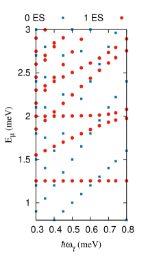
Figure 1: (Color online) Energy spectrum $E_{\mu}$ of the quantum wire versus the photon energy ($\hbar\omega_{\gamma}$), 0ES (blue rectangles) are zero-electron states, and 1ES (red circles) are one-electron states. The electron-photon coupling strength is $g_{\gamma}=0.05$ meV and the photons are linearly polarized in the $x$-direction. The magnetic field is $B=0.1~{}{\rm T}$, and $\hbar\Omega_{0}=2.0~{}{\rm meV}$.

In addition, the state between the ground state and the first-excited state is the one-photon replica of the ground state that is located between $1.5\text{-}2.0$ meV for the selected range of the photon energy. The one photon replica state at $\hbar\omega_{\gamma}=0.3$ meV is located at $\sim 1.55$ meV while the same state at $\hbar\omega_{\gamma}=0.74$ meV is seen at $\sim 1.99$ meV. Since the photon energy at $0.74$ meV is approximately equal to the energy spacing between the ground-state and the first-excited state, the electronics system is then close to a resonance with the photon field.

To demonstrate the transport properties we first present in Fig. 2 the heat current versus the chemical potential $\mu=\mu_{L}=\mu_{R}$ without a photon (w/o ph) cavity (blue squares), and with a photon cavity for the off-resonance case (red circles), and resonance (green diamonds) at time $t=220$ ps. The HC is plotted for the three lowest energy states at $E_{0}=1.25$, $E_{1}=1.99$ and $E_{2}=3.23$ meV, respectively. The vertical lines (violet lines) display the location of a resonance of the leads with the aforementioned three states. In the absence of the photon field, the HC is zero at the resonance energy states and has positive value between the resonance energy states. The positivity in HC can be explained by Eq. (2). Below the energy of each resonant state, meaning that the chemical potential is less than the energy of the state ($\mu<E_{\alpha}$), the first part of Eq. (2), ($\hat{\alpha}|\dot{\hat{\rho}}_{S}|\hat{\beta}$), is positive and the second part of equation, ($E_{\alpha}-\mu$), is also positive. Therefore, a positive value of HC is obtained. But, for energy above a resonant state when ($\mu>E_{\alpha}$) the first and the second part of the Eq. (2) are both negative giving a positive value of HC. In addition, the HC is zero at resonance state because $E_{\alpha}=\mu$.

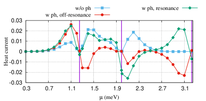
Figure 2: (Color online) Heat current as a function of the chemical potential $\mu=\mu_{L}=\mu_{R}$ plotted at time $t=220$ ps without a photon (w/o ph) cavity (blue squares), and with a photon cavity for the case of off-resonance (red circles), and resonance (green diamonds) at time $t=220$ ps. The temperature of the left (right) lead is fixed at $T_{\rm h}=6.38$ K ($T_{\rm c}=0.58$ K) implying thermal energy $k_{B}T_{\rm h}=0.55$ meV ($k_{B}T_{\rm c}=0.05$ meV), respectively. Therefore, the thermal energy of the system $k_{B}\Delta T=k_{B}T_{\rm h}-k_{B}T_{\rm c}=0.5$ meV. The vertical lines (violet lines) display the location of a resonance of the leads with the three lowest states including the ground state, the first-excited state and the second-excited state at $E_{\mu}=1.25$, $1.99$ and $3.23$ meV, respectively. The photons are linearly polarized in the $x$-direction and the electron-photon coupling strength $g_{\gamma}=0.15$. The photon cavity is assumed to have one photon initially $N_{\gamma}=1$. The magnetic field is $B=0.1~{}{\rm T}$, and $\hbar\Omega_{0}=2.0~{}{\rm meV}$.

When we consider the QW system coupled to a cavity-photon field, the HC gives us a different interesting picture. The HC can assume negative values due to the dressed electron-photon states in both the off-resonance ($\hbar\omega_{\gamma}=0.3$ meV) and the resonance ($\hbar\omega_{\gamma}=0.74$ meV) regimes. In these cases, photon replica states participate to the transport. For instance, above the first-exited state at the energy $2.1$ meV, the first photon replica of the first-exited state participates to the transport leading to the negative HC.

Figure 3 shows the thermoelectric current (TEC) versus the chemical potential $\mu=\mu_{L}=\mu_{R}$ without a photon (w/o ph) cavity (blue squares), and with a photon cavity for the case of $\hbar\omega_{\gamma}<k_{\rm B}\Delta{\rm T}$ (golden circles), and $\hbar\omega_{\gamma}>k_{\rm B}\Delta{\rm T}$ (red triangles) at time $t=220$ ps. At this time point, the system is in the late transient regime close to a steady state.

The current is essentially governed by the difference between the two Fermi functions of the external leads. The thermoelectric current is generated when the Fermi functions of the leads have the same chemical potential but different step width. One can explain the TEC of the system without the photon cavity as the following: The TEC becomes zero in two cases. First, when the two Fermi functions are equal to $0.5$ (half filling) and in the second one both Fermi functions are $0$ or $1$ (integer filling) [9, 4]. Therefore, the TEC is approximately zero at $\mu=1.25$ meV (blue squares) in the case of the system without the photon cavity corresponding to half filling of the ground state [21]. The TEC is approximately zero at $\mu=0.1$ and $1.99$ meV for the integer filling of occupation 0 and 1, respectively.

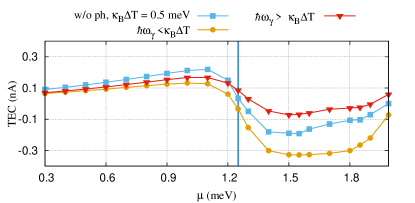
Figure 3: (Color online) TEC as a function of the chemical potential $\mu=\mu_{L}=\mu_{R}$ plotted at time $t=220$ ps without photon cavity (blue squares), and with photon cavity for the case of $\hbar\omega_{\gamma}<k_{\rm B}\Delta{\rm T}$ with $\hbar\omega_{\gamma}=0.3$ meV (golden circles), $\hbar\omega_{\gamma}>k_{\rm B}\Delta{\rm T}$ with $\hbar\omega_{\gamma}=0.74$ meV (red triangles). The temperature of the left (right) lead is fixed at $T_{\rm h}=6.38$ K ($T_{\rm c}=0.58$ K) implying thermal energy $k_{B}T_{\rm h}=0.55$ meV ($k_{B}T_{\rm c}=0.05$ meV), respectively. Therefore, the thermal energy of the system $k_{B}\Delta T=k_{B}T_{\rm h}-k_{B}T_{\rm c}=0.5$ meV. The vertical line (blue line) displays the location a resonance of the leads with the ground state. The photons are linearly polarized in the $x$-direction and the electron-photon coupling strength $g_{\gamma}=0.15$. The magnetic field is $B=0.1~{}{\rm T}$, and $\hbar\Omega_{0}=2.0~{}{\rm meV}$.

We consider the quantum wire coupled to a photon field with initially one photon in the cavity in the $x$-polarization. We assume two different regimes. First, when the photon energy is smaller than the thermal energy ($\hbar\omega_{\gamma}<k_{\rm B}\Delta{\rm T}$) in which the photon and the thermal energies are assumed to be $0.3$ and $0.5$ meV, respectively. In this case the TEC is suppressed in “positive” and enhanced in “negative” part as is shown in Fig. 3 (golden circles). The enhancement of TEC here is due to participation of one photon replica of the ground state around $E_{\mu}=1.55$ meV at $\hbar\omega_{\gamma}=0.3$ meV (Fig. 1) to the electron transport instead of the ground state itself. Generally, we expect no change in the TEC in the presence of a photon field here because the thermal energy is higher than the photon energy, i.e. the thermal smearing could be expected to prevent changes in the TEC. But, the one photon replica state strongly participates in the transport leading to an increase in the TEC.

This inspires us to try the opposite: We increase the photon energy to $0.74$ meV and keep the thermal energy at $0.5$ meV. The photon energy is now approximately equal to the energy spacing between the ground state and the first-excited state of the the quantum wire as is clearly seen in Fig. 1 at $\hbar\omega_{\gamma}=0.74$ meV. Therefore, the electronic system is almost in a resonance with the photon cavity, but under the condition of $\hbar\omega_{\gamma}>k_{\rm B}\Delta{\rm T}$ we now see in (Fig. 3 - red triangles) that the TEC is suppressed in both the “positive” and “negative” values due to the Rabi splitting. In this case, the following states contribute to the transport: The ground state, the one- and two-photon replica states of the ground state, and the second excited state. The contribution of these states marks the presence of Rabi oscillations. Consequently, suppression of TEC in the system is observed [21].

Now, we tune the thermal energy and keep the photon energy. The TEC versus thermal energy without photon cavity (blue circles), and with photon cavity for the case of $\hbar\omega_{\gamma}=0.3$ meV (golden diamonds), and $\hbar\omega_{\gamma}=0.74$ meV (red triangles) at $t=220$ ps is shown in Fig. 4.

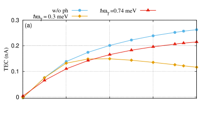
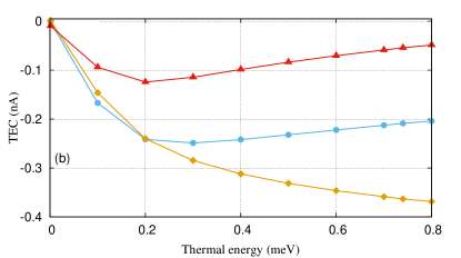
Figure 4: (Color online) TEC as a function of the chemical potential $\mu=\mu_{L}=\mu_{R}$ at time $t=220$ ps is plotted below the GS at $\mu=1.1$ meV (a) and above the GS at $\mu=1.4$ meV (b) shown in Fig. 1 in the case of the system without the cavity (blue circles), and with the cavity for the photon energy $\hbar\omega_{\gamma}=0.3$ meV (golden diamonds), and $\hbar\omega_{\gamma}=0.74$ (red triangles). The photon is linearly polarized in the $x$-direction and the electron-photon coupling strength $g_{\gamma}=0.15$ meV. The temperature of the right lead is fixed at $T_{\rm c}=0.58$ K implying thermal energy $k_{B}T_{\rm c}=0.05$ meV, and the temperature of the left lead is tuned. The magnetic field is $B=0.1~{}{\rm T}$, and $\hbar\Omega_{0}=2.0~{}{\rm meV}$.

Figure 4(a) shows the TEC below the ground state at $\mu=1.1$ meV and Fig. 4(b) presents the TEC above the ground state at $\mu=1.4$ meV. In the presence of the photon field, we see the same trends for the properties of the TEC mentioned above occurring for different values of thermal energies. For instance, if the photon energy is $\hbar\omega_{\gamma}=0.3$ meV (golden diamonds) the TEC is almost unchanged up to $k_{\rm B}\Delta{\rm T}=0.2$ meV. In addition, the rate of reduction of the TEC at $\mu=1.1$ meV is almost equal to the rate of increasing of the TEC at $\mu=1.4$ meV after $0.3$ meV. For photon energy $0.74$ meV (red triangles), the rate of increasing of the TEC at $\mu=1.1$ meV is slower than the rate of reduction of the TEC at $\mu=1.4$ meV. As we have mentioned above, in the resonance photon energy regime ( $0.74$ meV) several states contribute to the electron transport such as the ground state, the one- and two-photon replica states of the ground state, and the second excited state. At high thermal energy, the charging of few of these states such as the ground state is getting weaker. This leads to a stronger influence of the Rabi oscillation between other contributing states. Therefore, the TEC at $\mu=1.4$ meV is more suppressed around $\hbar\omega_{\gamma}=0.74$ meV.

In order to show further the influence of the photon field on TEC, we tune the electron-photon coupling strength. Figure 5 demonstrates the energy spectrum $E_{\mu}$ versus the electron-photon coupling strength $g_{\gamma}$, 0ES (green squares) are zero-electron states, 1ES (red circles) are one-electron states, and the horizontal lines (blue dotted lines) show the location of the the two lowest one-electron states in resonance with the leads with. The photon energy is $0.74$ meV.

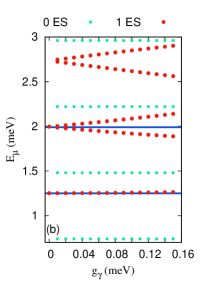
Figure 5: (Color online) Energy spectrum of the quantum wire versus electron-photon coupling strength $g_{\gamma}$. 0ES (golden circles) are zero-electron states, 1ES (blue squares) are one-electron states and the horizontal lines (red lines) display the location of the resonances of the leads with the three lowest one-electron states in the case of the resonance photon field ($\hbar\omega_{\gamma}=0.74$ meV). The photons are linearly polarized in the $x$-direction. The magnetic field is $B=0.1~{}{\rm T}$, and $\hbar\Omega_{0}=2.0~{}{\rm meV}$.

We begin with vanishing electron-photon coupling strength $g_{\gamma}=0$ meV. Two one-electron states are observed in the selected range of the energy spectrum: The ground state and the first-excited state with energy values $E_{0}=1.25$ meV and $E_{1}=1.99$ meV, respectively. In the presence of the cavity with photon energy $\hbar\omega_{\gamma}\simeq E_{1}-E_{0}\simeq 0.74$ meV the one-photon replica of the ground state is formed near to the first-excited state indicating a resonance regime. Increasing the electron-photon coupling strength, more splitting between the one photon replicas of the ground state and the first-excited state are seen. The splitting here is the Rabi splitting. We should mention that the same splitting occurs between the two-photon replica of the ground state and the one-photon replica of the first-excited state between $2.5\text{-}3.0$ meV. Even though we refer to photon replicas here with a certain photon number the reader should have in mind that photon replicas are a perturbational view of dressed electron states, that close to a resonance do not have an integer number of photons associate with them. The dressed states generally include a linear combination of several of the eigenstates of the photon number operator.

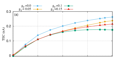
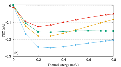
Figure 6: (Color online) TEC as a function of the thermal energy ($k_{\rm B}\Delta T$) at time $t=220$ p is plotted below ($\mu=1.1$ meV) (a) and above ($\mu=1.4$ meV) (b) the ground state shown in Fig. 1 for the system without the cavity $g_{\gamma}=0.0$ meV (blue circles), and with the cavity with the electron-photon coupling strength $g_{\gamma}=0.05$ (golden diamonds), $0.10$ (green squares), and $0.15$ meV (red triangles). The photon energy is $\hbar\omega_{\gamma}\simeq E_{1}-E_{1}\simeq 0.74$ meV (resonance regime) and the photons are linearly polarized in the $x$-direction. The temperature of the right lead is fixed at $T_{\rm c}=0.58$ K implying thermal energy $k_{B}T_{\rm c}=0.05$ meV, and the temperature of the left lead is tuned. The magnetic field is $B=0.1~{}{\rm T}$, and $\hbar\Omega_{0}=2.0~{}{\rm meV}$.

Figure 6 shows the TEC as a function of the thermal energy at time $t=220$ ps and $\mu=1.1$ meV (a) and $\mu=1.4$ (b) without a photon field $g_{\gamma}=0.0$ meV (blue circles) and with photon field for the electron-photon coupling strength $g_{\gamma}=0.05$ (golden diamonds), $0.1$ (green squares) and $0.15$ meV (red triangles) in the case of a nearly resonant photon field ($E_{1}-E_{0}\simeq\hbar\omega_{\gamma}=0.74$ meV). We fix the temperature of the right lead at $T_{c}=0.58$ K implying $k_{\rm B}T_{c}=0.05$ meV and tune the temperature of the left lead. Clearly seen is a reduction in the TEC with the electron-photon coupling strength. This reduction in the TEC is a direct consequence of the increased Rabi splitting shown in Fig. 5.

In a previous publication, we demonstrated the effects of electron-photon coupling strength on the TEC for a fixed value of thermal energy. We showed that Rabi splitting causes a reduction in the TEC with increasing electron-photon coupling strength. The stronger electron-photon coupling strength, the more reduction of the TEC was seen [21]. Here, we present the same influences of the electron-photon coupling but for different regimes of thermal energy. We show that it is not necessary to have a stronger reduction of the TEC for a stronger electron-photon coupling at high thermal energy especially between $0.5\text{-}0.8$ meV. In Fig. 6(b) it is seen that the TEC for $g_{\gamma}=0.1$ meV is higher than that of $g_{\gamma}=0.05$ meV between $0.5\text{-}0.8$ meV and the TEC for $g_{\gamma}=0.15$ meV is higher than that of $g_{\gamma}=0.1$ meV shown in Fig. 6(a). So, it demonstrates that the effects of the electron-photon coupling strength may influenced by the thermal energy in the system. Therefore, the influence of the Rabi-oscillation is modified by higher thermal energy in the system.

4 Conclusions

In this article we have shown photo-thermo-electric transport described by a quantum master equation, taking advantage of exact-diagonalization to include electron-photon interaction. We demonstrate that the heat current can be controlled in unexpected ways by a cavity-photon field. In addition, we show that the calculated thermoelectric current through the system depends on the ratio between the photon energy and the thermal energy, and the electron-photon coupling strength.

We observe that the effects of the cavity-photons on the thermoelectric current depend on the location of the chemical potential with respect to a particular state of the central system, and the ratio of the photon and the thermal energy. For low thermal energy the photons do enhance the thermoelectric current. As expected the largest effects are close to a Rabi resonance, when the electrons and photons are strongly coupled, and when the thermal energy is large. In this case, with the chemical potential of the leads just above the transport-resonant state the cavity photons reduce the transport current in the system. An off-resonant photon field enhances the transport current though. On the other hand, when the transport-resonant state is just below the chemical potential of the leads, the cavity-photons reduce the current for both cases, for nonresonant and resonant photons, but stronger in the latter case. The partially negative heat current is a result of a certain energy transfer from the photons to the electrons, as the system has not completely reached a steady state. The photons create an external perturbation on the electrons which behave like a slightly driven subsystem [22].

As a consequence, the thermoelectric current can be controlled in nanostructures using a quantized cavity photon field which may benefit energy harvesting in devices made thereof.

5 References

References

-
[1]
N. Nakpathomkun, H. Q. Xu, H. Linke, Phys. Rev. B 82 (2010) 235428.
doi:10.1103/PhysRevB.82.235428,
[link].
URL http://link.aps.org/doi/10.1103/PhysRevB.82.235428 -
[2]
V. Balachandran, R. Bosisio, G. Benenti,
Validity of the
Wiedemann-Franz law in small molecular wires, Phys. Rev. B 86 (2012)
035433.
doi:10.1103/PhysRevB.86.035433.
URL http://link.aps.org/doi/10.1103/PhysRevB.86.035433 -
[3]
Phys. Rev. B 84 (2011) 075410.
doi:10.1103/PhysRevB.84.075410,
[link].
URL http://link.aps.org/doi/10.1103/PhysRevB.84.075410 - [4] K. Torfason, A. Manolescu, S. I. Erlingsson, V. Gudmundsson, Thermoelectric current and Coulomb-blockade plateaus in a quantum dot, Physica E 53 (2013) 178–185.
- [5] A. Majumdar, Thermoelectricity in Semiconductor Nanostructure, Science 303 (2004) 777–778.
-
[6]
P. Trocha, J. Barnaś, Phys. Rev. B 85 (2012)
085408.
doi:10.1103/PhysRevB.85.085408,
[link].
URL http://link.aps.org/doi/10.1103/PhysRevB.85.085408 -
[7]
Y. S. Liu, X. F. Yang,
Enhancement
of thermoelectric efficiency in a double-quantum-dot molecular junction,
Journal of Applied Physics 108 (2).
doi:10.1063/1.3457124.
URL http://scitation.aip.org/content/aip/journal/jap/108/2/10.1063/1.3457124 - [8] T.-S. Kim, S. Hershfield, Phys. Rev. B 67 (2003) 165313.
-
[9]
M. B. Tagani, H. R. Soleimani,
,
Physica E 48 (2013) 36–41.
doi:10.1016/j.physe.2012.11.023.
URL http://www.sciencedirect.com/science/article/pii/S138694771200464X - [10] Sinova Jairo, Spin Seebeck effect: Thinks globally but acts locally, Nat. Mater. 9 (11) (2010) 880–881, 10.1038/nmat2880. doi:10.1038/nmat2880.
-
[11]
L.-C. Zhu, X.-D. Jiang, X.-T. Zu, H.-F. Lü, Physics Letters A 374 (41)
(2010) 4269–4273.
doi:10.1016/j.physleta.2010.08.048,
[link].
URL http://www.sciencedirect.com/science/article/pii/S0375960110010674 -
[12]
F. Chi, Y. Dubi,
Microwave-mediated
heat transport in a quantum dot attached to leads, Journal of Physics:
Condensed Matter 24 (14) (2012) 145301.
URL http://stacks.iop.org/0953-8984/24/i=14/a=145301 -
[13]
M. Tahir, P. Vasilopoulos, Phys. Rev. B 91 (2015) 115311.
doi:10.1103/PhysRevB.91.115311,
[link].
URL http://link.aps.org/doi/10.1103/PhysRevB.91.115311 - [14] W.-J. Gong, A. Du, Y. Wang, X.-H. Chen, Journal of the Physical Society of Japan 82 (1) (2013) 014603.
-
[15]
V. Gudmundsson, A. Sitek, N. R. Abdullah, C.-S. Tang, A. Manolescu,
Cavity-photon contribution
to the effective interaction of electrons in parallel quantum dots, Annalen
der Physik 528 (5) (2016) 394–403.
doi:10.1002/andp.201500298.
URL http://dx.doi.org/10.1002/andp.201500298 -
[16]
V. Gudmundsson, T. H. Jonsson, M. L. Bernodusson, N. R. Abdullah, A. Sitek,
H.-S. Goan, C.-S. Tang, A. Manolescu,
Regimes of radiative and
nonradiative transitions in transport through an electronic system in a
photon cavity reaching a steady state, Annalen der Physik 529 (1-2) (2017)
1600177–n/a, 1600177.
doi:10.1002/andp.201600177.
URL http://dx.doi.org/10.1002/andp.201600177 - [17] N. R. Abdullah, Magnetically and Photonically Tunable Double Waveguide Inverter, IEEE Journal of Quantum Electronics 52 (12) (2016) 1–6. doi:10.1109/JQE.2016.2626080.
- [18] N. R. Abdullah, C. S. Tang, A. Manolescu, V. Gudmundsson, Electron transport through a quantum dot assisted by cavity photons, Journal of Physics:Condensed Matter 25 (2013) 465302.
-
[19]
N. R. Abdullah, C.-S. Tang, A. Manolescu, V. Gudmundsson,
Optical
switching of electron transport in a waveguide-QED system, Physica E:
Low-dimensional Systems and Nanostructures 84 (2016) 280–284.
doi:10.1016/j.physe.2016.06.023.
URL http://www.sciencedirect.com/science/article/pii/S1386947716306749 - [20] V. Gudmundsson, O. Jonasson, C.-S. Tang, H.-S. Goan, A. Manolescu, Time-dependent transport of electrons through a photon cavity, Phys. Rev. B 85 (2012) 075306.
-
[21]
N. R. Abdullah, C.-S. Tang, A. Manolescu, V. Gudmundsson, ACS Photonics 3 (2)
(2016) 249–254.
arXiv:http://dx.doi.org/10.1021/acsphotonics.5b00532, doi:10.1021/acsphotonics.5b00532,
[link].
URL http://dx.doi.org/10.1021/acsphotonics.5b00532 -
[22]
N. R. Abdullah, C.-S. Tang, A. Manolescu, V. Gudmundsson,
Spin-dependent
heat and thermoelectric currents in a Rashba ring coupled to a photon
cavity, Physica E: Low-dimensional Systems and Nanostructures
95 (Supplement C) (2018) 102–107.
doi:10.1016/j.physe.2017.09.011.
URL http://www.sciencedirect.com/science/article/pii/S1386947717311372