Probing the structure of Kepler ZZ Ceti stars with full evolutionary models-based asteroseismology

Abstract

We present an asteroseismological analysis of four ZZ Ceti stars observed with Kepler: GD 1212, SDSS J113655.17+040952.6, KIC 11911480 and KIC 4552982, based on a grid of full evolutionary models of DA white dwarf stars. We employ a grid of carbon-oxygen core white dwarfs models, characterized by a detailed and consistent chemical inner profile for the core and the envelope. In addition to the observed periods, we take into account other information from the observational data, as amplitudes, rotational splittings and period spacing, as well as photometry and spectroscopy. For each star, we present an asteroseismological model that closely reproduce their observed properties. The asteroseismological stellar mass and effective temperature of the target stars are ($0.632\pm 0.027M_{\sun}$, $10737\pm 73$K) for GD 1212, ($0.745\pm 0.007M_{\sun}$, $11110\pm 69$K) for KIC 4552982, ($0.5480\pm 0.01M_{\sun}$, $12721\pm 228$K) for KIC1191480 and ($0.570\pm 0.01M_{\sun}$, $12060\pm 300$K) for SDSS J113655.17+040952.6. In general, the asteroseismological values are in good agreement with the spectroscopy. For KIC 11911480 and SDSS J113655.17+040952.6 we derive a similar seismological mass, but the hydrogen envelope is an order of magnitude thinner for SDSS J113655.17+040952.6, that is part of a binary system and went through a common envelope phase.

1 Introduction

ZZ Ceti (or DAV) variable stars constitute the most populous class of pulsating white dwarfs (WDs). They are otherwise normal DA (H-rich atmospheres) WDs located in a narrow instability strip with effective temperatures between $10\,500$ K and $12\,500$ K (e.g., Winget & Kepler, 2008; Fontaine & Brassard, 2008; Althaus et al., 2010b; Kepler & Romero, 2017) that show luminosity variations of up to $0.30$ mag caused by nonradial $g$-mode pulsations of low degree ($\ell\leq 2$) and periods between 70 and 1500 s. Pulsations are triggered by a combination of the $\kappa-\gamma$ mechanism acting at the basis of the hydrogen partial ionization zone (Dolez & Vauclair, 1981; Dziembowski & Koester, 1981; Winget et al., 1982) and the convective driving mechanism (Brickhill, 1991; Goldreich & Wu, 1999).

Asteroseismology of WDs uses the comparison of the observed pulsation periods with the adiabatic periods computed for appropriate stellar models. It allows us to learn about the origin, internal structure and evolution of WDs (Winget & Kepler, 2008; Althaus et al., 2010b; Fontaine & Brassard, 2008). In particular, asteroseismological analysis of ZZ Ceti stars provide strong constraints on the stellar mass, the thickness of the outer envelopes, the core chemical composition, and the stellar rotation rates. Furthermore, the rate of period changes of ZZ Ceti stars allows to derive the cooling timescale (Kepler et al., 2005b; Kepler, 2012; Mukadam et al., 2013), to study axions (Isern et al., 1992; Córsico et al., 2001; Bischoff-Kim et al., 2008; Córsico et al., 2012b, c, 2016), neutrinos (Winget et al., 2004; Córsico et al., 2014), and the possible secular rate of variation of the gravitational constant (Córsico et al., 2013). Finally, ZZ Ceti stars allow to study crystallization (Montgomery & Winget, 1999; Córsico et al., 2004, 2005; Metcalfe et al., 2004; Kanaan et al., 2005; Romero et al., 2013), to constrain nuclear reaction rates (e.g. ¹²C$(\alpha,\gamma)^{16}$O, Metcalfe et al., 2002), to infer the properties of the outer convection zones (Montgomery, 2005a, b, 2007), and to look for extra-solar planets orbiting these stars (Mullally et al., 2008).

Two main approaches have been adopted hitherto for WD asteroseismology. One of them employs stellar models with parametrized chemical profiles. This approach has the advantage that it allows a full exploration of parameter space to find the best seismic model (see, for details, Bischoff-Kim & Østensen, 2011; Bischoff-Kim et al., 2014; Giammichele et al., 2016, 2017b, 2017a). However, this method requires the number of detected periods to be larger to the number of free parameters in the model grid, which is not always the case for pulsationg DA stars. The other approach —the one we adopt in this paper— employs fully evolutionary models resulting from the complete evolution of the progenitor stars, from the ZAMS to the WD stage. Because this approach is more time consuming from the computational point of view, usually the model grid is not as thin or versatile as in the first approach. However, it involves the most detailed and updated input physics, in particular regarding the internal chemical structure from the stellar core to the surface, that is a crucial aspect for correctly disentangling the information encoded in the pulsation patterns of variable WDs. Specially, most structural parameters are set consistently by the evolution prior to the white dwarf cooling phase, reducing significantly the number of free parameters. The use of full evolutionary models has been extensively applied in asteroseismological analysis of hot GW Vir (or DOV) stars (Córsico et al., 2007a, b, 2008, 2009; Kepler et al., 2014; Calcaferro et al., 2016), V777 Her (DBV) stars (Córsico et al., 2012a; Bognár et al., 2014; Córsico et al., 2014), ZZ Ceti stars (Kepler et al., 2012; Romero et al., 2012, 2013), and Extremely low mass white dwarf variable stars (ELMV) (Calcaferro et al., 2017).

Out of the $\sim$170 ZZ Ceti stars known to date (Bognar & Sodor, 2016; Kepler & Romero, 2017), 48 are bright objects with $V<16$, and the remainder are fainter ZZ Ceti stars that have been detected with the Sloan Digital Sky Survey (SDSS) (Mukadam et al., 2004; Mullally et al., 2005; Kepler et al., 2005a, 2012; Castanheira et al., 2006, 2007, 2010, 2013). The list is now being enlarged with the recent discovery of pulsating WD stars within the Kepler spacecraft field, thus opening a new avenue for WD asteroseismology based on observations from space (see e.g. Hermes et al., 2017a). This kind of data is different from ground base photometry because it does not have the usual gaps due to daylight, but also different reduction techniques have to be employed to uncover the pulsation spectra of the stars observed with the Kepler spacecraft. In particular, after the two wheels stopped to function, known as the K2 phase, additional noise is introduced to the signal due to the shooting of the trusters with a timescale around six hours to correct the pointing. The ZZ Ceti longest observed by Kepler, KIC 4552982 (WD J1916+3938, $T_{\rm eff}=10\,860$ K, $\log g=8.16$), was discovered from ground-based photometry by Hermes et al. (2011). This star exhibits pulsation periods in the range $360-1500$ s and shows energetic outbursts (Bell et al., 2015). A second ZZ Ceti star observed with Kepler is KIC 11911480 (WD J1920+5017, $T_{\rm eff}=12\,160$ K, $\log g=7.94$), that exhibits a total of six independent pulsation modes with periods between 173 and 325 s (Greiss et al., 2014), typical of the hot ZZ Ceti stars (Clemens et al., 2000; Mukadam et al., 2006). Four of its pulsation modes show strong signatures of rotational splitting, allowing to estimate a rotation period of $\sim$3.5 days. The ZZ Ceti star GD 1212 (WD J2338$-$0741, $T_{\rm eff}=10\,980$ K, $\log g=7.995$, (Hermes et al., 2017a) was observed for a total of 264.5 hr using the Kepler (K2) spacecraft in two-wheel mode. (Hermes et al., 2014) reported the detection of 19 pulsation modes, with periods ranging from 828 to 1221 s. Recently Hermes et al. (2017a) analyzed the light curve and find a smaller number of real $m=0$ component modes in the spectra, which we will consider to performe our seismological analysis. Finally, there is the ZZ Ceti star SDSS J113655.17+040952.6 (J1136$+$0409), discovered by Pyrzas et al. (2015) and observed in detail by Hermes et al. (2015). This is the first known DAV variable WD in a post–common–envelope binary system. Recently, Greiss et al. (2016) reported additional ZZ Ceti stars in the Kepler mission field. Also, Hermes et al. (2017a) present photometry and spectroscopy for 27 ZZ Ceti stars observed by the Kepler space telescope, including the four objects analyzed here.

In this paper, we carry out an asteroseismological analysis of the first four published ZZ Ceti stars observed with Kepler by employing evolutionary DA WD models representative of these objects. We perform our study by employing a grid of full evolutionary models representative of DA WD stars as discussed in Romero et al. (2012) and extended toward higher stellar mass values in Romero et al. (2013). Evolutionary models have consistent chemical profiles for both the core and the envelope for various stellar masses, specifically calculated for asteroseismological fits of ZZ Ceti stars. The chemical profiles of our models are computed considering the complete evolution of the progenitor stars from the ZAMS through the thermally pulsing and mass-loss phases on the asymptotic giant branch (AGB). Our asteroseismological approach combines (1) a significant exploration of the parameter space $(M_{\star},T_{\rm eff},M_{\rm H})$, and (2) updated input physics, in particular, regarding the internal chemical structure, that is a crucial aspect for WD asteroseismology. In addition, the impact of the uncertainties resulting from the evolutionary history of progenitor star on the properties of asteroseismological models of ZZ Ceti stars has been assessed by De Gerónimo et al. (2017) and De Gerónimo et al. (2017b, submitted.). This adds confidence to the use of fully evolutionary models with consistent chemical profiles, and renders much more robust our asteroseismological approach.

The paper is organized as follows. In Sect. 2, we provide a brief description of the evolutionary code, the input physics adopted in our calculations and the grid of models employed. In Sect. 3, we describe our asteroseismological procedure and the application to the target stars. We conclude in Sect. 4 by summarizing our findings.

2 Numerical tools and models

2.1 Input physics

The grid of full evolutionary models used in this work was calculated with an updated version of the LPCODE evolutionary code (see Althaus et al., 2005, 2010a; Renedo et al., 2010; Romero et al., 2015, for details). LPCODE compute the evolution of single, i.e. non–binary, stars with low and intermediate mass at the Main Sequence. Here, we briefly mention the main input physics relevant for this work. Further details can be found in those papers and in Romero et al. (2012, 2013).

The LPCODE evolutionary code considers a simultaneous treatment of no-instantaneous mixing and burning of elements (Althaus et al., 2003). The nuclear network accounts explicitly for 16 elements and 34 nuclear reactions, that include $pp$ chain, CNO-cycle, helium burning and carbon ignition (Renedo et al., 2010). In particular, the ¹²C$(\alpha,\gamma)^{16}$O reaction rate, of special relevance for the carbon-oxygen stratification of the resulting WD, was taken from Angulo et al. (1999). Note that the ¹²C$(\alpha,\gamma)^{16}$O reaction rate is one of the main source of uncertainties in stellar evolution. By considering the computations of Kunz et al. (2002) for the ¹²C$(\alpha,\gamma)^{16}$O reaction rate, the oxygen abundance at the center can vary from 26% to 45% within the theoretical uncertainties, leading to a change in the period values up to $\sim 11$ s for a stellar mass of 0.548$M_{\sun}$ (De Gerónimo et al., 2017). We consider the occurrence of extra-mixing episodes beyond each convective boundary following the prescription of Herwig et al. (1997), except for the thermally pulsating AGB phase. We considered mass loss during the core helium burning and the red giant branch phases following Schröder & Cuntz (2005), and during the AGB and thermally pulsating AGB following the prescription of Vassiliadis & Wood (1993). During the WD evolution, we considered the distinct physical processes that modify the inner chemical profile. In particular, element diffusion strongly affects the chemical composition profile throughout the outer layers. Indeed, our sequences develop a pure hydrogen envelope with increasing thickness as evolution proceeds. Our treatment of time dependent diffusion is based on the multicomponent gas treatment presented in Burgers (1969). We consider gravitational settling and thermal and chemical diffusion of H, ³He, ⁴He, ¹²C, ¹³C, ¹⁴N and ¹⁶O (Althaus et al., 2003). To account for convection process we adopted the mixing length theory, in its ML2 flavor, with the free parameter $\alpha=1.61$ (Tassoul et al., 1990) during the evolution previous to the white dwarf cooling curve, and $\alpha=1$ during the white dwarf evolution. Last, we considered the chemical rehomogenization of the inner carbon-oxygen profile induced by Rayleigh-Taylor instabilities following Salaris et al. (1997).

The input physics of the code includes the equation of state of Segretain et al. (1994) for the high density regime complemented with an updated version of the equation of state of Magni & Mazzitelli (1979) for the low density regime. Other physical ingredients considered in LPCODE are the radiative opacities from the OPAL opacity project (Iglesias & Rogers, 1996) supplemented at low temperatures with the molecular opacities of Alexander & Ferguson (1994). Conductive opacities are those from Cassisi et al. (2007), and the neutrino emission rates are taken from Itoh et al. (1996) and Haft et al. (1994).

Cool WD stars are expected to crystallize as a result of strong Coulomb interactions in their very dense interior (van Horn, 1968). In the process two additional energy sources, i.e. the release of latent heat and the release of gravitational energy associated with changes in the chemical composition of carbon-oxygen profile induced by crystallization (Garcia-Berro et al., 1988a, b; Winget et al., 2009) are considered self-consistently and locally coupled to the full set of equations of stellar evolution. The chemical redistribution due to phase separation has been considered following the procedure described in Montgomery & Winget (1999) and Salaris et al. (1997). To assess the enhancement of oxygen in the crystallized core we used the azeotropic-type formulation of Horowitz et al. (2010).

2.2 Model grid

The DA WD models used in this work are the result of full evolutionary calculations of the progenitor stars, from the ZAMS, through the hydrogen and helium central burning stages, thermal pulses, the planetary nebula phase and finally the white dwarf cooling sequences, using the LPCODE code. The metallicity value adopted in the main sequence models is $Z=0.01$. Most of the sequences with masses $\lesssim 0.878M_{\sun}$ were used in the asteroseismological study of 44 bright ZZ Ceti stars by Romero et al. (2012), and were extracted from the full evolutionary computations of Althaus et al. (2010a) (see also Renedo et al., 2010). Romero et al. (2013) extended the model grid toward the high–mass domain. They computed five new full evolutionary sequences with initial masses on the ZAMS in the range $5.5-6.7M_{\sun}$ resulting in WD sequences with stellar masses between $0.917$ and $1.05M_{\sun}$.

The values of stellar mass of our complete model grid are listed in Column 1 of Table LABEL:masses, along with the hydrogen (Column 2) and helium (Column 3) content as predicted by standard stellar evolution, and carbon $(X_{\rm C})$ and oxygen $(X_{\rm O})$ central abundances by mass in Columns 4 and 5, respectively. Additional sequences, shown in italic, were computed for this work. The values of stellar mass of our set of models covers all the observed pulsating DA WD stars with a probable carbon-oxygen core. The maximum value of the hydrogen envelope (column 2), as predicted by progenitor evolution, shows a strong dependence on the stellar mass and it is determined by the limit of H–burning. It ranges from $3.2\times 10^{-4}M_{\star}$ for $M_{\star}=0.493M_{\sun}$ to $1.4\times 10^{-6}M_{\sun}$ for $M_{\star}=1.050M_{\sun}$, with a value of $\sim 1\times 10^{-4}M_{\star}$ for the average-mass sequence of $M_{\star}\sim 0.60M_{\sun}$.

Table 1: The main characteristics of our set of DA WD models. Sequences with the mass value in italic where computed for this work. The sequence with 0.493 $M_{\sun}$ comes from a full evolutionary model, while the remaining four sequences were the result of the interpolation process described in Romero et al. (2013).

$M_{\star}/M_{\sun}$	$-\log(M_{\rm H}/M_{\star})$	$-\log(M_{\rm He}/M_{\star})$	$X_{\rm C}$	$X_{\rm O}$
0.493	3.50	1.08	0.268	0.720
0.525	3.62	1.31	0.278	0.709
0.548	3.74	1.38	0.290	0.697
0.560	3.70	1.42	0.296	0.691
0.570	3.82	1.46	0.301	0.696
0.593	3.93	1.62	0.283	0.704
0.609	4.02	1.61	0.264	0.723
0.632	4.25	1.76	0.234	0.755
0.660	4.26	1.92	0.258	0.730
0.674	4.35	1.97	0.280	0.707
0.690	4.46	2.04	0.303	0.684
0.705	4.45	2.12	0.326	0.661
0.721	4.50	2.14	0.328	0.659
0.745	4.62	2.18	0.330	0.657
0.770	4.70	2.23	0.332	0.655
0.800	4.84	2.33	0.339	0.648
0.837	5.00	2.50	0.347	0.640
0.878	5.07	2.59	0.367	0.611
0.917	5.41	2.88	0.378	0.609
0.949	5.51	2.92	0.373	0.614
0.976	5.68	2.96	0.374	0.613
0.998	5.70	3.11	0.358	0.629
1.024	5.74	3.25	0.356	0.631
1.050	5.84	2.96	0.374	0.613

Our parameter space is build up by varying three quantities: stellar mass $(M_{\star})$, effective temperature $(T_{\rm eff})$ and thickness of the hydrogen envelope $(M_{\rm H})$. Both the stellar mass and the effective temperature vary consistently as a result of the use of a fully evolutionary approach. On the other hand, we decided to vary the thickness of the hydrogen envelope in order to expand our parameter space. The choice of varying $M_{\rm H}$ is not arbitrary, since there are uncertainties related to physical processes operative during the TP-AGB phase leading to uncertainties on the amount of hydrogen remaining on the envelope of WD stars (see Romero et al., 2012, 2013; Althaus et al., 2015, for a detailed justification of this choice). In order to get different values of the thickness of the hydrogen envelope, we follow the procedure described in Romero et al. (2012, 2013). For each sequence with a given stellar mass and a thick H envelope, as predicted by the full computation of the pre-WD evolution (Column 2 in Table LABEL:masses), we replaced ¹H with ⁴He at the bottom of the hydrogen envelope. This is done at high effective temperatures ($\lesssim 90\,000$ K), so the transitory effects caused by the artificial procedure are completely washed out when the model reaches the ZZ Ceti instability strip. The resulting values of hydrogen content for different envelopes are shown in Figure 1 for each mass. The orange thick line connects the values of $M_{\rm H}$ predicted by our stellar evolution (Column 2, Table LABEL:masses).

Other structural parameters do not change considerably according to standard evolutionary computations. For example, Romero et al. (2012) showed that the remaining helium content of DA WD stars can be slightly lower (a factor of $3-4$) than that predicted by standard stellar evolution only at the expense of an increase in mass of the hydrogen-free core $(\sim 0.2M_{\sun})$. The structure of the carbon-oxygen chemical profiles is basically fixed by the evolution during the core helium burning stage and is not expected to vary during the following single star evolution (we do not consider possible merger episodes). The chemical structure of the carbon-oxygen core is affected by the uncertainties inherent to the ¹²C$(\alpha,\gamma)^{16}$O reaction rate. A detailed assessing of the impact of this reaction rate on the precise shape of the core chemical structure and the pulsational properties is presented by De Gerónimo et al. (2017).

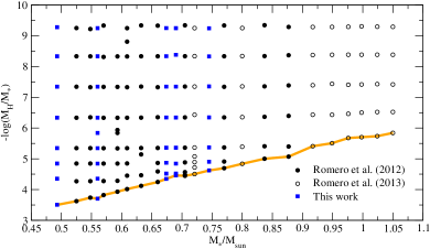
Figure 1: Grid of DA WD evolutionary sequences considered in this work in the $M_{\star}/M_{\sun}$ vs $-\log(M_{\rm H}/M_{\star})$ plane. Each symbol corresponds to a sequence of models representative of WD stars characterized by a given stellar mass and hydrogen envelope mass. Filled circles correspond to the evolutionary sequences computed in Romero et al. (2012), hollow circles correspond to sequences computed in Romero et al. (2013) and filled squares correspond to the sequences computed in this work. The orange line connects the sequences with the maximum values for the thickness of the hydrogen envelope, predicted by our evolutionary computations.

Summarizing, we have available a grid of $\sim 290$ evolutionary sequences characterized by a detailed and updated input physics, in particular, regarding the internal chemical structure, that is a crucial aspect for WD asteroseismology.

2.3 Pulsation computations

In this study the adiabatic pulsation periods of nonradial $g$-modes for our complete set of DA WD models were computed using the adiabatic version of the LP-PUL pulsation code described in Córsico & Althaus (2006). This code is based on the general Newton-Raphson technique that solves the full fourth–order set of equations and boundary conditions governing linear, adiabatic, non-radial stellar oscillations following the dimensionless formulation of Dziembowski (1971). We used the so-called “Ledoux-modified” treatment to assess the run of the Brunt-Väisalä frequency ($N$; see Tassoul et al., 1990), generalized to include the effects of having three different chemical components varying in abundance. This code is coupled with the LPCODE evolutionary code.

The asymptotic period spacing is computed as in Tassoul et al. (1990):

$$\Delta\Pi_{\ell}^{\rm a}=\frac{2\pi^{2}}{\sqrt{\ell(\ell+1)}}\left[\int_{r_{1}}^{r_{2}}\frac{N}{r}dr\right]^{-1}$$ (1)

where $N$ is the Brunt-Vïsälä frequency, and $r_{1}$ and $r_{2}$ are the radii of the inner and outer boundary of the propagation region, respectively. When a fraction of the core is crystallized, $r_{1}$ coincides with the radius of the crystallization front, which is moving outward as the star cools down, and the fraction of crystallized mass increases.

We computed adiabatic pulsation $g$-modes with $\ell=1$ and 2 and periods in the range 80–2000 s. This range of periods corresponds (on average) to $1\lesssim k\lesssim 50$ for $\ell=1$ and $1\lesssim k\lesssim 90$ for $\ell=2$.

3 Asteroseismological results

For our target stars, KIC 4552982, KIC 11911480, J113655.17+040952.6 and GD 1212, we searched for an asteroseismological representative model that best matches the observed periods of each star. To this end, we seek for the theoretical model that minimizes the quality function given by Castanheira & Kepler (2009):

$$S=\frac{1}{N}\sqrt{\sum^{N}_{i=1}\frac{[\Pi_{k}^{th}-\Pi_{i}^{obs}]^{2}\times A_{i}}{\sum^{N}_{i=1}Ai}}$$ (2)

where $N$ is the number of the observed periods in the star under study, $\Pi_{k}^{\rm th}$ and $\Pi_{i}^{\rm obs}$ are the theoretical and observed periods, respectively and $A_{i}$ is the amplitude of the observed mode. The numerical uncertainties for $M_{\star},T_{\rm eff}$, and $\log(L_{\star}/L_{\sun})$ were computed by using the following expression (Zhang et al., 1986; Castanheira & Kepler, 2008):

$$\sigma_{j}^{2}=\frac{d_{j}^{2}}{(S-S_{\rm 0})},$$ (3)

where $S_{\rm 0}\equiv\Phi(M_{\star}^{\rm 0},M_{\rm H}^{\rm 0},T_{\rm eff}^{\rm 0})$ is the minimum of the quality function $S$ which is reached at $(M_{\star}^{\rm 0},M_{\rm H}^{\rm 0},T_{\rm eff}^{\rm 0})$ corresponding to the best-fit model, and $S$ is the value of the quality function when we change the parameter $j$ (in this case, $M_{\star},M_{\rm H}$, or $T_{\rm eff}$) by an amount $d_{j}$, keeping fixed the other parameters. The quantity $d_{j}$ can be evaluated as the minimum step in the grid of the parameter $j$. The uncertainties in the other quantities ($L_{\star},R_{\star},g$, etc) are derived from the uncertainties in $M_{\star}$ and $T_{\rm eff}$. These uncertainties represent the internal errors of the fitting procedure.

3.1 KIC 11911480

The DA WD star KIC 11911480 was discovered to be variable from ground-based observations as a part of the RATS-Kepler survey (Ramsay et al., 2014). These observations revealed a dominant periodicity of $\sim 290$ s. The star was observed by Kepler in the short-cadence mode in quarters 12 and 16 (Q12 and Q16) and a total of 13 periods were detected (see Table 2 of Greiss et al., 2014). Of these, 5 periods were identified as $m=0$ components of rotational triplets and the remainder ones as $m=\pm 1$ components. Greiss et al. (2014) also determine the spectroscopic values of the atmospheric parameters using spectra from the double-armed Intermediate resolution Spectrograph (ISIS) on the William Herschel Telescope (WHT) and the pure hydrogen atmosphere models, with MLT/$\alpha$ = 0.8, from Koester (2010). As a result, they obtained $T_{\rm eff}=12\,160\pm 250$ K and $\log g=7.94\pm 0.10$, after applying the 3D convection correction from Tremblay et al. (2013). By employing our set of DA WD evolutionary tracks, we derive $M_{\star}=0.574\pm 0.05M_{\sun}$. Greiss et al. (2016) determine the atmospheric parameter using the same spectra but considering the atmosphere models from Tremblay et al. (2011) with MLT/$\alpha$=0.8. The result was $T_{\rm eff}=11\,580\pm 140$ K and $\log g=7.96\pm 0.04$, also corrected by 3D convection. From these parameters we obtain a stellar mass of $M_{\star}=0.583\pm 0.02M_{\sun}$. The “hot” solution obtained by Greiss et al. (2014) is in better agreement with the short periods observed in this star.

Table 2: Columns 1,2 and 3: The observed $m=0$ periods of KIC 11911480 to be employed as input of our asteroseismological analysis, with the $\ell$ value fixed by the detection of rotational splitting components. Columns: 4, 5, 6 and 7: The theoretical periods with their corresponding harmonic degree, radial order and rotation coefficient for our best fit model for KIC11911480.

Observations			Asteroseismology
$\Pi_{i}^{\rm obs}$ [s]	$A_{i}$ [mma]	$\ell$	$\Pi_{i}^{\rm Theo}$	$\ell$	$k$	$C_{\rm k\ell}$
290.802	2.175	1	290.982	1	4	0.44332
259.253	0.975	1	257.923	1	3	0.47087
324.316	0.278	1	323.634	1	5	0.36870
172.900	0.149	-	170.800	2	4	0.14153
202.569	0.118	-	204.085	2	5	0.12244

In our analysis, we employ only the five periods shown in Table LABEL:modos, which correspond to the five $m=0$ observed periods of Q12 and Q16. The quoted amplitudes are those of Q16. We assume that the three large amplitude modes with periods 290.802 s, 259.253 s, and 324.316 are dipole modes because they are unambiguously identified with the central components of triplets ($\ell=1$).

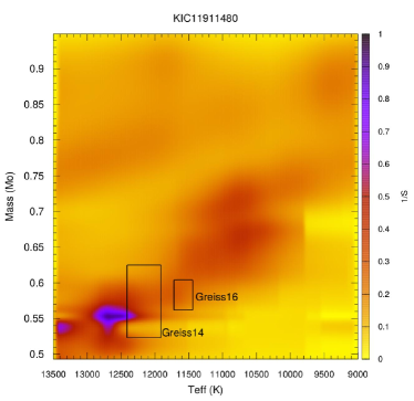
Figure 2: Projection on the effective temperature vs. stellar mass plane of the inverse of the quality function S for KIC11911480. The hydrogen envelope thickness value for each stellar mass corresponds to the sequence with the lowest value of the quality function for that stellar mass. The box indicates the stellar mass and effective temperature values obtained from spectroscopy by Greiss et al. (2016).

Our results are shown in Figure 2 which shows the projection of the inverse of the quality function S on the $T_{\rm eff}-M_{\star}/M_{\sun}$ plane. The boxes correspond to the spectroscopic determinations from Greiss et al. (2014) and Greiss et al. (2016). For each stellar mass, the value of the hydrogen envelope thickness corresponds to the sequence with the lower value of the quality function for that stellar mass. The color bar on the right indicates the value of the inverse of the quality function $S$. The asteroseismological solutions point to a stellar mass between 0.54 and 0.57$M_{\sun}$, with a blue edge-like effective temperature, in better agreement with the spectroscopic determination from Greiss et al. (2014), as can be seen from Figure 2. The parameters of the model characterizing the minimum of $S$ for KIC 11911480 are listed in Table LABEL:tabla-soluciones, along with the spectroscopic parameters. Note that the seismological effective temperature is quite high, even higher than the classical blue edge of the instability strip (Gianninas et al., 2011). However, the extension of the instability strip is being redefined with some ZZ Ceti stars characterized with high effective temperatures. For instance, Hermes et al. (2017b) reported the existence of the hottest known ZZ Ceti, EPIC 211914185, with $T_{\rm eff}=13\,590\pm 340$ and $M_{\star}=0.87\pm 0.03M_{\sun}$. Also, we can be overestimating the effective temperature obtained from asteroseismology.

Table 3: List of parameters characterizing the best fit model obtained for KIC 11911480. Also, we list the spectroscopic values from Greiss et al. (2014) and Greiss et al. (2016). The quoted uncertainties are the intrinsic uncertainties of the seismological fit.

Greiss et al. (2014)	Greiss et al. (2016)	LPCODE
$M_{\star}=0.574\pm 0.05M_{\sun}$	$M_{\star}=0.583\pm 0.05M_{\sun}$	$M_{\star}=0.548\pm 0.01M_{\sun}$
$T_{\rm eff}=12\,160\pm 250$ K	$T_{\rm eff}=11\,580\pm 140$ K	$T_{\rm eff}=12\,721\pm 228$ K
$\log g=7.94\pm 0.10$	$\log g=7.96\pm 0.04$	$\log g=7.88\pm 0.05$
		$\log(L/L_{\sun})=-2.333\pm 0.032$
		$R/R_{\sun}=0.014\pm 0.001$
		$M_{\rm H}/M_{\sun}=2.088\times 10^{-4}$
		$M_{\rm He}/M_{\sun}=4.19\times 10^{-2}$
		$X_{\rm C}=0.290,X_{\rm O}=0.697$
		$P_{\rm rot}=3.36\pm 0.2$ d
		$S=1.13$ s

The list of theoretical periods corresponding to the model in Table LABEL:tabla-soluciones is shown in Table LABEL:modos. Also listed are the harmonic degree, the radial order and the $C_{\rm k\ell}$ rotation coefficient. Using the frequency spacing $\Delta f$ for the three $\ell=1$ modes from Table 2 of Greiss et al. (2014) and the rotation coefficients we estimated a rotation period of $3.36\pm 0.2$ days.

3.2 J113655.1+040952.6

J1136$+$0409 (EPIC 201730811) was first observed by Pyrzas et al. (2015) as part of a search for ZZ Ceti stars among the WD $+$ MS binaries and it turn out to be the only variable in a post common envelope binary from the sample studied by these authors. This star was spectroscopically identified as a WD $+$ dM from its SDSS spectrum. The surface parameters were determined by Rebassa-Mansergas et al. (2012) by model-atmosphere fits to the Balmer absorption lines after subtracting an M star spectrum, giving $T_{\rm eff}=11\,700\pm 150$ K and $\log g=7.99\pm 0.08$. Pulsations were confirmed by a short run with the ULTRACAM instrument mounted on the 3.5m New Technology Telescope by Pyrzas et al. (2015). Hermes et al. (2015) reported the results from a 78 days observation run in August 2014 with the Kepler spacecraft in the frame of the extended Kepler mission, K2 Campaign 1. In addition, these authors obtained high S/N spectroscopy with SOAR to refine the determinations of the atmospheric parameters. They used two independent grids of synthetic spectra to fit the Balmer lines: the pure hydrogen atmosphere models and fitting procedure described by Gianninas et al. (2011), and the pure hydrogen atmosphere models from Koester (2010). Both grids employ the ML2/$\alpha=0.8$ prescription of the mixing-length theory (Gianninas et al., 2011). By applying the 3D correction from Tremblay et al. (2013) they obtained $T_{\rm eff}=12\,579\pm 250$ K and $\log g=7.96\pm 0.05$ for the values obtained with the Gianninas et al. (2011) fit and $T_{\rm eff}=12\,083\pm 250$ K and $\log g=8.02\pm 0.07$ for the Koester (2010) fit. From these values, we computed the stellar mass of J113655.17+040952.6 by employing our set of evolutionary sequences, and obtained $M_{\star}=0.585\pm 0.03M_{\sun}$ and $M_{\star}=0.616\pm 0.06M_{\sun}$, respectively. Recently, Hermes et al. (2017a) determined the atmospheric parameters using the same spectra as Hermes et al. (2015) and the MLT$/\alpha$=0.8 models from Tremblay et al. (2011), resulting in $T_{\rm eff}=12\,480\pm 170$ K and $\log g=7.956\pm 0.0435$, similar to those obtained by using the model grid from Gianninas et al. (2011). As in the case of KIC 11911480, in our analysis we consider both spectroscopic determinations from Gianninas et al. (2011) and Koester (2010) with the corresponding 3D correction.

Table 4: Columns 1,2 and 3: Observed periods of J113655.17+040952.6 to be employed as input of our asteroseismological analysis with the $\ell$ value fixed for three modes, according to Hermes et al. (2015). Columns 4, 5, 6 and 7: The theoretical periods with their corresponding harmonic degree, radial order and rotation coefficient for our best fit model for J113655.17+040952.6.

Observation			Asteroseismology
$\Pi_{i}^{\rm obs}$	$A_{i}$ (ppt)	$\ell$	$\Pi_{i}^{\rm Theo}$	$\ell$	$k$	$C_{\rm k\ell}$
279.443	2.272	1	277.865	1	3	0.44222
181.283	1.841	-	185.187	1	2	0.37396
162.231	1.213	1	161.071	1	1	0.48732
344.277	0.775	1	344.218	1	5	0.47552
201.782	0.519	-	195.923	2	4	0.14507

From the analysis of the light curve, Hermes et al. (2015) found 12 pulsation frequencies, 8 of them being components of rotational triplets ($\ell=1$). Only 7 frequencies were identified with $m=0$ components. Further analysis of the light curve revealed that the two modes with the lower amplitudes detected were not actually real modes but nonlinear combination frequencies. We consider 5 periods for our asteroseismic study, which are listed in Table LABEL:J1136-obs. According to Hermes et al. (2015), the modes with periods 279.443 s, 162.231 s and 344.277 s are the central $m=0$ components of rotational triplets. In particular, the 344.277 s period is not detected but it corresponds to the mean value of the frequencies of 2848.17 and 2761.10 $\mu$Hz, identified as the prograde and retrograde components, respectively. We assume that the harmonic degree of the periods identified as $m=0$ components of triplets (Hermes et al., 2015) is $\ell=1$.

Table 5: List of parameters characterizing the best fit model obtained for J113655.17+040952.6 along with the spectroscopic determinations from Hermes et al. (2015) using the atmosphere models from Gianninas et al. (2011) (G2011) and Koester (2010) (K2010). The quoted uncertainties are the intrinsic uncertainties of the seismological fit.

Hermes et al. (2015)		LPCODE
G2011	K2010
$M_{\star}=0.585\pm 0.03M_{\sun}$	$M_{\star}=0.616\pm 0.06M_{\sun}$	$M_{\star}=0.570\pm 0.01M_{\sun}$
$T_{\rm eff}=12\,579\pm 250$ K	$T_{\rm eff}=12\,083\pm 250$ K	$T_{\rm eff}=12\,060\pm 300$ K
$\log g=7.96\pm 0.05$	$\log g=8.02\pm 0.07$	$\log g=7.95\pm 0.07$
		$\log(L/L_{\sun})=-2.414\pm 0.045$
		$R/R_{\sun}=0.0132\pm 0.002$
		$M_{\rm H}/M_{\sun}=1.774\times 10^{-5}$
		$M_{\rm He}/M_{\sun}=3.50\times 10^{-2}$
		$X_{\rm C}=0.301,X_{\rm O}=0.696$
		$P_{\rm rot}=2.6\pm 1$ hr
		$S=2.83$ s

The results for our asteroseismological fits are shown in figure 3, which shows the projection of the inverse of the quality function $S$ on the $T_{\rm eff}-M_{\star}/M_{\sun}$ plane. The hydrogen envelope thickness value for each stellar mass corresponds to the sequence with the lowest value of the quality function. We show the spectroscopic values from Hermes et al. (2015) with boxes. As can be seen from this figure, we have a family of minimum around $\sim 0.57M_{\sun}$ and $12\,000$ K. The structural parameters characterizing the best fit model are listed in Table LABEL:sol-J1136 while the list of theoretical periods are listed in the last four columns of Table LABEL:J1136-obs. Note that, in addition to the three modes for which we fixed the harmonic degree to be $\ell=1$ (279.443 s, 162.231 s, and 344.407 s), the mode with period 181.283 s, showing the second largest amplitude, is also fitted by a dipole theoretical mode. Our seismological stellar mass is somewhat lower than the values shown in Table LABEL:J1136-obs, but still compatible with the spectroscopic determinations. The effective temperature is a blue edge-like value closer to the determinations using Koester (2010) atmosphere models. In addition, we obtain a hydrogen envelope $\sim 20\%$ thicker than the seismological results presented in Hermes et al. (2015). Since the central oxygen composition is not a free parameter in our grid, the oxygen abundance at the core of the WD model is fixed by the previous evolution, and has a value of $X_{\rm O}=0.696$, much lower than the value found by Hermes et al. (2015) of $X_{\rm O}=0.99$. Note that even taking into account the uncertainties in the ¹²C$(\alpha,\gamma)$O¹⁶ reaction rate given in Kunz et al. (2002) the abundance of oxygen can only be as large as $X_{\rm O}=0.738$ (De Gerónimo et al., 2017). Results from deBoer et al. (2017) are also consistent with a $\sim$10% uncertainty in the oxygen central abundance. Finally, we computed the rotation coefficients $C_{k\ell}$ (last column in Table LABEL:J1136-obs) and used the identified triplets to derived a mean rotation period of $2.6\pm 0.1$ hr.

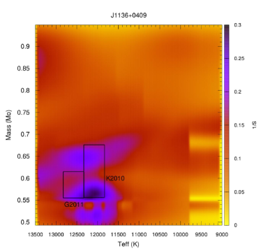
Figure 3: Projection on the effective temperature vs. stellar mass plane of the inverse of the quality function $S$ for J113655.17+040952.6. The box indicates the spectroscopic determinations from Hermes et al. (2015).

3.3 KIC 4552982

KIC 4552982, also known as SDSS J191643.83+393849.7, was identified in the Kepler Mission field through ground-based time series photometry by Hermes et al. (2011). These authors detected seven frequencies of low-amplitude luminosity variations with periods between $\sim 800$ s and $\sim 1450$ s. The stellar mass and effective temperature determinations are $T_{\rm eff}=11\,129\pm 115$ K and $\log g=8.34\pm 0.06$ that corresponds to $M_{\star}=0.82\pm 0.04M_{\sun}$. By applying the 3D convection correction Bell et al. (2015) obtained $T_{\rm eff}=10\,860\pm 120$ K and $\log g=8.16\pm 0.06$ that corresponds to $M_{\star}=0.693\pm 0.047M_{\sun}$. Similar results were reported by Hermes et al. (2017a) using the same spectra and the model grid from Tremblay et al. (2011), $T_{\rm eff}=10\,950\pm 160$ K, $\log g=8.113\pm 0.053$ and $M_{\star}=0.665\pm 0.030M_{\sun}$.

Bell et al. (2015) presented photometric data for KIC 4552982 spanning more than 1.5 years obtained with Kepler, making it the longest pseudo-continuous light curve ever recorded for a ZZ Ceti star. They identify 20 periods from $\sim 360$ s to $\sim 1500$ s (see Table LABEL:KIC45-obs). From the list, it is apparent that the three modes around $\sim 361$ s are very close, and probably they are part of a $\ell=1$ rotation multiplet (Bell et al., 2015). Therefore, we can consider the observed period of $361.58$ s as the $m=0$ component of the triplet and assume that this period is associated to a dipole ($\ell=1$) mode. Bell et al. (2015) have searched for a possible period spacing in their list of periods. They found two sequences with evenly space periods, being the period separations of $41.9\pm 0.2$ s and $20.97\pm 0.02$, identified as possible $\ell=1$ and $\ell=2$ sequences, respectively. By using the strong dependence of the asymptotic period spacing with the stellar mass, we can estimate the stellar mass of KIC 4552982 as $M_{\star}\sim 0.8M_{\sun}$ and thick hydrogen envelope.

Table 6: Observed periods of KIC 4552982 according to Bell et al. (2015). The amplitudes correspond to the square root of the Lorentzian height listed in Table 2 of Bell et al. (2015). Column 3 shows the theoretical periods correspondign to the Best fit model (BFM) (see. Table LABEL:sol-KIC455 or first row in Table LABEL:sol-sip) with the corresponding harmonic degree and radial order ($\ell,k$). Column 4 list the theoretical periods, and ($\ell$,$k$), for the second best fit model (see second row of Table LABEL:sol-sip).

$\Pi_{i}^{\rm obs}$	$A_{i}$ (mma)	$\Pi_{i}^{\rm Theo}$ (BFM)	$\Pi_{i}^{\rm Theo}$
360.53	$\cdots$	$\cdots$	$\cdots$
361.58	$\cdots$	361.20 (1,5)	361.25 (1,6)
362.64	0.161	$\cdots$	$\cdots$
788.24	0.054	788.57 (1,14)	788.35 (1,7)
828.29	0.142	829.27(1,15)	831.17 (1,18)
866.11	0.163	870.34 (1,16)	873.94 (1,19)
907.59	0.137	907.91 (1,17)	917.99 (1,20)
950.45	0.157	944.62 (1,18)	949.16 (1,21)
982.23	0.090	984.00 (2,33)	982.14 (1,22)
1014.24	0.081	1018.11 (2,34)	1021.97 (2,40)
1053.68	0.056	1048.47 (2,35)	1049.40 (2,41)
1100.87	0.048	1098,72 (2,37)	1095.46 (2,43)
1158.20	0.074	1155.79 (2,39)	1154.85 (1,26)
1200.18	0.042	1201.51 (1,23)	1200.26 (2,51)
1244.73	0.048	1245.58 (1,24)	1245.22 (2,49)
1289.21	0.115	1290.06 (1,25)	1292.77 (1,29)
1301.73	0.084	1299.40 (2,44)	1295.67 (2,51)
1333.18	0.071	1333.14 (2,45)	1340.16 (2,53)
1362.95	0.075	1358.30 (2,46)	1362.91 (1,31)
1498.32	0.079	1502.55 (2,51)	1496.03 (2,59)

We start our analysis of KIC 4552982 by carrying out an asteroseismological period fit employing the 18 modes identified as $m=0$. In addition to assure that the mode with $\sim 361.6$ s is the $m=0$ component of a triplet, Bell et al. (2015) also identify the modes with period between 788 and 950 s as $\ell=1$ modes. These modes are separated by a nearly constant period spacing and have similar amplitudes (see Fig. 10 Bell et al., 2015), except for the mode with 788.24 s. Then we consider all five periods as dipole modes and fix the harmonic degree to $\ell=1$. We allow the remainder periods to be associated to either $\ell=1$ or $\ell=2$ modes, without restriction at the outset.

In Fig. 4 we show the projection on the $T_{\rm eff}-M_{\star}$ plane of $1/S$ corresponding to the seismological fit of KIC 4552982.The hydrogen envelope value corresponds to the sequence with the lowest value of the quality function for that stellar mass. We include in the figure the spectroscopic determinations of the effective temperature and stellar mass for KIC 4552982 with (Spec-3D) and without (Spec-1D) correction from Tremblay et al. (2013) with the associated uncertainties as a box. From this figure two families of solutions can be identified: A ”hot” family with $T_{\rm eff}>12\,000$K and stellar mass between 0.55 and 0.65$M_{\sun}$ and ”cool” family with $T_{\rm eff}\sim 11\,000$K and stellar mass $\sim 0.72M_{\sun}$. This star has a rich period spectra, with 18 pulsation periods showing similar amplitudes. Then, with no amplitude–dominant mode, the period spacing would have a strong influence on the quality function and thus in the seismological fit. Note that the asymptotic period spacing increases with decreasing mass and effective temperature, then the strip in figure 4 formed by the two families correspond to a ”constant period spacing” strip. We disregard the ”hot” family of solutions based on the properties of the observed period spectrum, with many long excited periods with high radial order, which is compatible with a cool ZZ Ceti star. In addition, a high $T_{\rm eff}$ is in great disagreement with the spectroscopic determinations, as can be seen from Fig. 4.

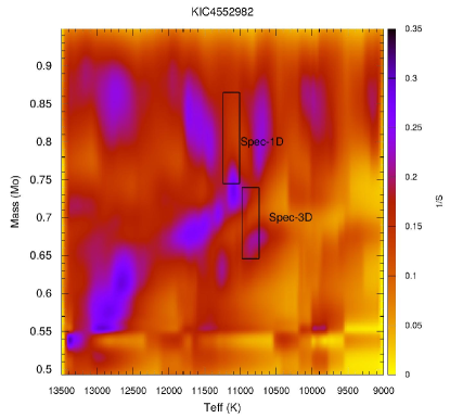
Figure 4: Projection on the effective temperature vs. stellar mass of $1/S$ for KIC 4552982. We fixed the harmonic degree for the six modes with the shortest periods ($\ell=1$). Spectroscopic determinations with and without the 3D convection correction are also depicted as boxes.

The parameters of our best fit model for KIC 4552982 are listed in Table LABEL:sol-KIC455, along with the spectroscopic determinations with and without the 3D convection correction. This solution is in better agreement with the spectroscopic determinations without the 3D-corrections, as can be see from figure 4. Using the data from the frequency separation for rotational splitting of $\sim 10\mu Hz$ and the corresponding rotation coefficient $C_{k\ell}=0.48612$ we obtain a rotation period of $\sim 15\pm 1$ h. The list of theoretical periods and their values of $\ell$ and $k$ corresponding to this model are listed in the first row of Table LABEL:sol-sip. Also listed are the asymptotic period spacing for dipole and quadrupole modes.

The model with the minimum value of the quality function within the box corresponding to spectroscopic determinations with 3D-corrections (Spec-3D) shows an stellar mass of $0.721M_{\sun}$ and an effective temperature of $10\,875$ K. However the period-to-period fit is not as good, with a value of the quality function of 4.87 s. The theoretical periods for this model are listed in the second row of Table LABEL:sol-sip.

Table 7: List of parameters characterizing the best fit model obtained for KIC 4552982 along with the spectroscopic determinations from Bell et al. (2015) and Hermes et al. (2011). The quoted uncertainties are the intrinsic uncertainties of the seismological fit.

Hermes et al. (2011)	Bell et al. (2015)	LPCODE
$M_{\star}=0.805\pm 0.06M_{\sun}$	$M_{\star}=0.693\pm 0.047M_{\sun}$	$M_{\star}=0.745\pm 0.007M_{\sun}$
$T_{\rm eff}=11\,129\pm 115$ K	$T_{\rm eff}=10\,860\pm 120$ K	$T_{\rm eff}=11\,110\pm 69$ K
$\log g=8.34\pm 0.06$	$\log g=8.16\pm 0.06$	$\log g=8.26\pm 0.05$
		$\log(L/L_{\sun})=-2.815\pm 0.011$
		$R/R_{\sun}=0.0105\pm 0.0002$
		$M_{\rm H}/M_{\sun}=4.70\times 10^{-9}$
		$M_{\rm He}/M_{\sun}=6.61\times 10^{-3}$
		$X_{\rm C}=0.330,X_{\rm O}=0.657$
		$P_{\rm rot}=15\pm 1$ hr
		$S=3.45$ s

Table 8: Seismological solution for KIC 4552982 considering the 18 modes identified as $m=0$ components. The harmonic degree for the modes with periods between 361.58 s and 950 s is fixed to be $\ell=1$ at the outset, in agreement with the identification and the possible period spacing proposed by Bell et al. (2015).

$M_{\star}/M_{\sun}$	$M_{\rm H}/M_{\star}$	$T_{\rm eff}$ [K]	$\Delta\Pi_{\ell=1}$	$\Delta\Pi_{\ell=2}$	$S$ (s)
0.745	$4.70\times 10^{-9}$	$11\,110$	50.50	29.16	3.45
0.721	$3.13\times 10^{-5}$	$10\,875$	43.48	25.10	5.05

If we assume that the mean period spacing of 41.9 s derived by Bell et al. (2015) for KIC 4552982 is associated to the asymptotic period spacing for dipole modes, then only the asteroseismological solution of $0.721M_{\sun}$ is compatible with this star. This is illustrated in the upper panel of Fig. 5, in which we depict the dipole asymptotic period spacing (red line) for the $0.721M_{\sun}$ model, along with the observed forward period spacing ($\equiv\Pi_{k+1}-\Pi_{k}$) of KIC 4552982 (blue squares connected with thin lines) in terms of the pulsation periods. In addition, the $\ell=1$ theoretical forward period-spacing values are displayed with black circles. The lower panel shows the situation for the best fit model with $M_{\star}=0.745M_{\sun}$. It is apparent that for this model, the asymptotic period spacing is too long as to be compatible with the observed mean period spacing of 41.9 s of KIC 4552982. However, in these cases the forward period spacing values of the model are in very good agreement with the period spacing values observed in the star. In summary, the two selected models can be considered as compatible with KIC 4552982 concerning either the mean period spacing of 41.9 s, or the individual forward period spacing values exhibited by the star. However, from the period–to–period fit the best fit model corresponds to that with stellar mass of $0.745M_{\sun}$ (first row in Table LABEL:sol-sip).

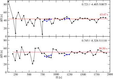
Figure 5: The forward period spacing in terms of the periods for the theoretical models (black circles) listed in Table LABEL:sol-sip. In each panel we specify the stellar mass, the hydrogen mass [$\log(M_{\rm H}/M_{\star})$] and the effective temperature in K. The asymptotic period spacing is depicted as a red horizontal line. Blue squared connected with thin lines represent the forward period spacing of the modes identified as $\ell=1$ modes by Bell et al. (2015), assuming that these modes have consecutive radial orders.

3.4 GD 1212

GD 1212 was reported to be a ZZ Ceti star by Gianninas et al. (2006), showing a dominant period at $\sim 1161$ s. Spectroscopic values of effective temperature and gravity from Gianninas et al. (2011) are $T_{\rm eff}=11270\pm 165$ K and $\log g=8.18\pm 0.05$, using their ML2/$\alpha=0.8$ atmosphere models. By applying the 3D corrections of Tremblay et al. (2013) we obtain $T_{\rm eff}=10\,970\pm 170$ K and $\log g=8.03\pm 0.05$. Hermes et al. (2017a) determine the atmospheric parameters of GD 1212 using SOAR spectra and obtained $T_{\rm eff}=10\,980\pm 140$ K and $\log g=7.995\pm 0.040$, by applying the atmosphere model grid from Tremblay et al. (2011). The ML2/$\alpha=0.8$ model atmosphere fits to the photometry of GD 1212 lead to a somewhat lower effective temperature and a higher gravity, $T_{\rm eff}=10\,940\pm 320$ K and $\log g=8.25\pm 0.03$ (Giammichele et al., 2012). By employing our set of DA WD evolutionary tracks, we derive the stellar mass of GD 1212 from its observed surface parameters, being $M_{\star}=0.619\pm 0.027M_{\sun}$, $M_{\star}=0.600\pm 0.021M_{\sun}$ and $M_{\star}=0.747\pm 0.023M_{\sun}$, corresponding to the two 3D corrected spectroscopic and photometric determinations of $T_{\rm eff}$ and $\log g$, respectively. From a total of 254.5 hr of observations with the Kepler spacecraft, Hermes et al. (2014) reported the detection of 19 pulsation modes with periods between 828.2 and 1220.8 s (see first column of Table 9). Both the discovery periods and those observed with the Kepler spacecraft are consistent with a red edge ZZ Ceti pulsator, with effective temperatures $\sim 11\,000$ K. Hermes et al. (2017a) reanalyzed the data using only the final 9 days of the K2 engineering data. After concluding that the star rotates with a period of $\sim 6.9$ days, they found five modes corresponding to $m=0$ components of multiples, along with two modes with no identified harmonic degree. These period values for the seven modes are listed in columns 3 and 4 of Table 9.

Table 9: List of periods for GD 1212 corresponding to Hermes et al. (2014) (column 1) and Hermes et al. (2017a) (columns 2 and 3)

Hermes et al. (2014)		This work
$\Pi_{i}^{\rm obs}$	$\Pi_{i}^{\rm obs}$	HWHM	$\ell$
$\cdots$	369.85	0.348	?
$828.19\pm 1.79$	826.26	0.593	2
$842.96\pm 1.02$	842.90	0.456	1
$849.13\pm 0.76$	$\cdots$	$\cdots$	-
$857.51\pm 0.86$	$\cdots$	$\cdots$	-
$871.06\pm 2.13$	$\cdots$	$\cdots$	-
$956.87\pm 4.91$	958.39	0.870	?
$987.00\pm 3.73$	$\cdots$	$\cdots$	-
$1008.07\pm 1.20$	$\cdots$	$\cdots$	-
$1025.31\pm 2.26$	$\cdots$	$\cdots$	-
$1048.19\pm 4.01$	$\cdots$	$\cdots$	-
$1063.08\pm 4.13$	1063.1	0.970	2
$1086.12\pm 3.27$	1085.86	0.558	2
$1098.36\pm 1.65$	$\cdots$	$\cdots$	-
$1125.37\pm 3.01$	$\cdots$	$\cdots$	-
$1147.12\pm 3.19$	$\cdots$	$\cdots$	-
$1166.67\pm 4.81$	$\cdots$	$\cdots$	-
$1180.40\pm 4.02$	$\cdots$	$\cdots$	-
$1190.53\pm 2.28$	1190.5	0.789	1
$1220.75\pm 7.15$	$\cdots$	$\cdots$	-

In this work we use the list of periods shown in the column 3 of Table 9 (Hermes et al., 2017a) to perform our asteroseismological study. Two modes are identified as dipole modes. Then we fix the harmonic degree to be $\ell=1$ for these modes (see Table 9), and allow the remaining modes to be associated to dipoles or quadrupoles. To find the best fit models we looked for those models associated with minima in the quality function $S$, to ensure that the theoretical periods are the closest match to the observed values. The results from our fit are shown in Figure 6. The spectroscopic values from Gianninas et al. (2011), with 3D convection correction from Tremblay et al. (2013) and from photometry (Giammichele et al., 2012) are depicted with black boxes. From this figure, a well defined family of solutions can be seen around $M_{\star}=0.63M_{\sun}$ and $T_{\rm eff}=10\,750$ K. The structure parameter characterizing the best fit model for GD 1212 are listed in Table LABEL:GD1212-model. The theoretical periods and the corresponding harmonic degree and radial order are listed in Table LABEL:GD1212-teo. Note that, appart from the two modes for which we fixed the harmonic degree to be $\ell=1$, the modes identified by Hermes et al. (2017a) as $\ell=2$ modes, are also quadrupole modes in our best fit model, as the two modes with no defined harmonic degree.

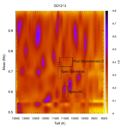
Figure 6: Projection on the effective temperature vs. stellar mass plane of the inverse of the quality function $S$ for GD 1212. Open rectangles indicate the values obtained from spectroscopy Gianninas et al. (2011), with 3D convection correction from Tremblay et al. (2013) (Hermes et al., 2014) and from photometry Giammichele et al. (2012).

Table 10: List of parameters characterizing the best fit model obtained for GD 1212 along with the spectroscopic determinations with and without 3D convection correction, and photometry. The quoted uncertainties are the intrinsic uncertainties of the seismological fit.

Hermes et al. (2014)	LPCODE
$M_{\star}=0.600\pm 0.027M_{\sun}$	$M_{\star}=0.632\pm M_{\sun}$
$T_{\rm eff}=10\,980\pm 140$ K	$T_{\rm eff}=10\,737\pm 70$ K
$\log g=8.03\pm 0.05$	$\log g=8.05\pm 0.04$
	$\log(L/L_{\sun})=-2.737\pm 0.008$
	$R/R_{\sun}=0.0123\pm 0.0003$
	$M_{\rm H}/M_{\sun}=7.582\times 10^{-5}$
	$M_{\rm He}/M_{\sun}=1.74\times 10^{-2}$
	$X_{\rm C}=0.234,X_{\rm O}=0.755$
	$S=1.32$ s

Table 11: The theoretical periods with their corresponding harmonic degree and radial order for our best fit model for GD 1212.

$\Pi_{i}^{\rm Theo}$	$\ell$	$k$
369.342	2	12
826.191	2	30
841.005	1	17
956.400	2	35
1064.42	2	39
1086.32	2	40
1191.45	1	25

We also performed a seismological analysis based on the periods reported by Hermes et al. (2014). Using the period spacing for $\ell=1$ modes of $\Delta\Pi=41.5\pm 2.5$ s determined by Hermes et al. (2014) and the spectroscopic effective temperature we estimated the stellar mass by comparing this value to the theoretical asymptotic period spacing corresponding to canonical sequences, listed in Table LABEL:masses. As a result, we obtained $M_{\star}=(0.770\pm 0.067)M_{\sun}$. Then, we performed an asteroseismological fit using two independent codes: LP-PUL and WDEC. From the fits with LP-PUL we obtained solutions characterized by high stellar mass of $\sim 0.878M_{\sun}$, 15-20% higher than the spectroscopic value, and $T_{\rm eff}$ around $11\,200$ and $11\,600$ K. The best fit model obtained with WDEC also shows a high mass of $0.815M_{\sun}$ and an effective temperature of $11\,000$ K. The high mass solutions are expected given the large number of periods and the period spacing required to fit all modes simultaneously, since the period spacing decreases when mass increases and thus there are more theoretical modes in a given period range. Finally, all possible solutions are characterized by thick hydrogen envelopes.

3.4.1 Atmospheric parameters of GD 1212

From the seismological study of GD 1212 using an improved list of observed mode we obtained a best fit model characterized by $M_{\star}=0.632M_{\sun}$ and $T_{\rm eff}=10\,737$ K. The asteroseismic stellar mass is somewhat higher than the spectroscopic determinations from Gianninas et al. (2011) with the 3D convection corrections from Tremblay et al. (2013), set at $0.619\pm 0.027M_{\sun}$. On the other hand, from our asteroseismological study of GD 1212 considering the period list from Hermes et al. (2014) we obtained solutions characterized with a high stellar mass. Using the model grid computed with LPCODE we obtained an stellar mass $\sim 0.88M_{\sun}$. Considering the asymptotic period spacing estimated by Hermes et al. (2014) of $\Delta\Pi=41.5\pm 2.5$ s and the spectroscopic effective temperature $10\,970\pm 170$ K the stellar mass drops to $0.770\pm 0.067M_{\sun}$. Also, using the WDEC model grid, we also obtained a high mass solution, with a stellar mass of $0.815M_{\sun}$. The process of extracting the pulsation periods for GD 1212, and perhaps for the cool ZZ Ceti stars showing a rich pulsation spectra, appears to be somewhat dependent of the reduction process (Hermes et al., 2017a). Then, we must search for other independent data to uncover the most compatible period spectra and thus seismological solution. To this end, we search for spectroscopic and photometric determinations of the effective temperature and surface gravity in the literature. We used observed spectra taken by other authors and re-determine the atmospheric parameters using up-to-date atmosphere models. Our results are listed in table 12. In this table, determinations of the atmospheric parameters using spectroscopy are in rows 1 to 7, while rows 8 to 11 correspond to determinations based on photometric data (see Table LABEL:foto) and parallax from Subasavage et al. (2009). We also determined the stellar mass using our white dwarf cooling models. Finally, we include the determinations with and without applying the 3D convection correction for the spectroscopic determinations.

Table 12: Determination of GD 1212 atmosphere parameters from different authors. Rows 1 to 7 correspond to determinations based on spectroscopic data, while rows 8 to 11 correspond to determinations based on photometric data (see Table LABEL:foto) and parallax determinations from Subasavage et al. (2009).
Notes: 1- Gianninas et al. (2011) using spectroscopy. 2- Hermes et al. (2017a) using spectroscopy 3- Kawka et al. (2004) using spectroscopy. 4- Kawka et al. (2007), spectrum from Kawka et al. (2004). 5-Spectrum from Kawka et al. (2004) fitted with models from Kawka & Vennes (2012). 6- Spectrum from Kawka et al. (2004) fitted with models from Koester (2010). 7- Spectrum from Gianninas et al. (2011) fitted with models from Koester (2010). 8- Photometric result from Giammichele et al. (2012). 9- Photometric data from SDSS, GALEX and 2MASS and parallax fitted with models from Kawka & Vennes (2012). 10- Photometric data from SDSS and GALEX and parallax fitted with models from Koester (2010). 11- Photometric data BVIJHK colors and GALEX and parallax fitted with models from Koester (2010).

	Ref.	$T_{\rm eff}$ [K]	$\log g$	$M_{\star}/M_{\sun}$	$T_{\rm eff}$ [K]	$\log g$	$M_{\star}/M_{\sun}$
		non - 3D			3D - corrected
1	Gianninas et al. (2011)	$11\,270\pm 165$	$8.18\pm 0.05$	$0.705\pm 0.040$	$10\,970\pm 170$	$8.03\pm 0.05$	$0.619\pm 0.027$
2	Hermes et al. (2017a)	$11\,280\pm 140$	$8.144\pm 0.040$	$0.684\pm 0.023$	$10\,980\pm 140$	$7.995\pm 0.04$	$0.600\pm 0.021$
3	Kawka et al. (2004)	$10\,960\pm 75$	$8.20\pm 0.10$	$0.714\pm 0.087$	$11\,012\pm 75$	$7.98\pm 0.10$	$0.592\pm 0.075$
4	Kawka et al. (2007)	$11\,010\pm 210$	$8.05\pm 0.15$	$0.630\pm 0.100$	$11\,093\pm 210$	$7.85\pm 0.15$	$0.526\pm 0.093$
5	This paper	$11\,130\pm 200$	$8.12\pm 0.10$	$0.669\pm 0.078$	$11\,228\pm 200$	$7.92\pm 0.10$	$0.561\pm 0.065$
6	This paper	$11\,770\pm 75$	$8.27\pm 0.05$	$0.764\pm 0.048$	$11\,445\pm 103$	$8.17\pm 0.07$	$0.698\pm 0.062$
7	This paper	$11\,573\pm 23$	$8.04\pm 0.01$	$0.627\pm 0.009$	$11\,251\pm 33$	$7.94\pm 0.02$	$0.573\pm 0.014$
8	Giammichele et al. (2012)	$10\,940\pm 320$	$8.25\pm 0.03$	$0.747\pm 0.023$	$\cdots$	$\cdots$	$\cdots$
9	This paper	$10\,860\pm 30$	$8.25\pm 0.02$	$0.747\pm 0.022$	$\cdots$	$\cdots$	$\cdots$
10	This paper	$10\,963\pm 114$	$8.23\pm 0.04$	$0.734\pm 0.039$	$\cdots$	$\cdots$	$\cdots$
11	This paper	$11\,153\pm 193$	$8.28\pm 0.21$	$0.771\pm 0.182$	$\cdots$	$\cdots$	$\cdots$

We compare the determinations of the effective temperature and the stellar mass for GD 1212 using the different techniques discussed above. The results are summarized in Figure 7. The boxes correspond to the parameter range from the different determinations using spectroscopy, with and without the 3D convection correction, and photometry (see references in the figure). Our best fit model is depicted by a solid circle, while the solutions corresponding to the asteroseismological fits using the period list from Hermes et al. (2014) are depicted as solid squares. Our best fit model is in good agreement with the spectroscopic determinations within the uncertainties. The stellar mass is somewhat lower than that from photometric determinations but the effective temperature is in excellent agreement, and consistent with a cool ZZ Ceti star. Then we conclude that the list of periods shown in the right columns of table 9 are compatible with the photometric and spectroscopic determinations and is most likely to be the the real period spectra.

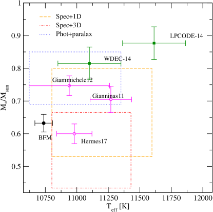
Figure 7: Determinations of the effective temperature and stellar mass for GD 1212. The boxes correspond to the parameter range from the different determinations using spectroscopy, with (Spec+3D) and without (Spec+1D) the 3D convection correction, and photometry combined with the parallax (Phot+parallax). Determinations from Gianninas et al. (2011), Hermes et al. (2014) and Giammichele et al. (2012) are plotted as references as hollow circles. The solid black circle represents the position of the best fit model obtained in this work. Solid squares corresponds to the seismological solutions using the period list from Hermes et al. (2014) obtained using the model grid computed with LPCODE (LPCODE-14) and WDEC (WDEC-14).

Table 13: Photometric data for GD 1212.

	mag	err	source
u	13.653	0.039	SDSS
g	13.267	0.200	SDSS
r	13.374	0.018	SDSS
i	13.547	0.018	SDSS
z	13.766	0.021	SDSS
B	13.440	0.061	Holberg et al. (2002)
V	13.260	0.048	Holberg et al. (2002)
I	13.240	0.028	Subasavage et al. (2009)
J	13.339	0.029	Cutri et al. (2003)
H	13.341	0.023	Cutri et al. (2003)
K	13.35	0.031	Cutri et al. (2003)
FUV	15.714	0.150	GALEX
NUV	14.228	0.182	GALEX
parallax (mas)	62.7	1.7	Subasavage et al. (2009)

4 Summary and conclusions

In this paper we have presented an asteroseismological study of the first four published ZZ Ceti stars observed with the Kepler spacecraft. We have employed an updated version of the grid of fully evolutionary models presented in Romero et al. (2012, 2013). In our seismological analysis, along with the period list, we consider additional information coming from the detection of rotational frequency splittings or sequences of possible consecutive radial order modes, i.e., period spacing value. We summarize our results below:

• For KIC 11911480, we find a seismological mass in good agreement with the spectroscopic mass. Regarding the effective temperature, we find a higher value from seismology than spectroscopy. It is important to note that the atmospheric parameters determined from spectroscopy and asteroseismology can differ beyond the systematic uncertainties, since spectroscopy is measuring the top of the atmosphere and asteroseismology is probing the base of the convection zone. In particular, the effective temperature characterizing our seismological models is related to the luminosity and radius of the model, while that from spectroscopy can vary from layer to layer. Also, using the rotation coefficients and the frequency spacings found by Greiss et al. (2014) for three identified dipole modes, we obtained a rotation period of $3.36\pm 0.2$ days.

• In the case of J113655.17+040952.6, we found a seismological mass of $0.570M_{\sun}$ and effective temperature of $12\,060$ K. The seismological mass is lower than that from spectroscopy but in agreement within the uncertainties. The seismological effective temperature is $\sim 300$ K lower than the spectroscopic value from Gianninas et al. (2011) with 3D correction but in excellent agreement with that using Koester (2010) atmosphere models. Finally, we determine a rotation period of 2.6 d from the frequency spacings for the three $\ell=1$ modes identified by Hermes et al. (2015) and the rotational coefficients corresponding to our best fit model.

• KIC 4552982 is a red–edge ZZ Ceti with 18 detected periods. In this case we found a seismological solution with a stellar mass of 0.745$M_{\sun}$ and effective temperature $11\,110$ K, compatible with spectroscopic determinations. The asymptotic period spacing for dipole modes for our seismological solution (50.50 s) seems long as compared to the period spacing estimated by Bell et al. (2015) (41.9 s). However the forward period spacing itself is compatible with the observations, as shown in figure 5, since the asymptotic regime is reached for periods longer than 2000 s. Finally, our best fit model is characterized by a very thin hydrogen envelope mass, which could be related to the outburst nature reported by Bell et al. (2015). Whether this is a common characteristic between all the outburst ZZ Cetis or not is beyond the scope of this work and will be studied in a future paper.

• Finally, GD 1212 is also a red–edge ZZ Ceti with 9 independent pulsation periods. We obtained a best fit model characterized by $M_{\star}=0.632M_{\sun}$ and $T_{\rm eff}=10\,922$ K. The stellar mass is somewhat higher than the spectroscopic value, but the effective temperature is in excellent agreement. We also fit the period list reported in Hermes et al. (2014) and obtained a high stellar mass solution ($\sim 0.88M_{\sun}$). However, other determinations of the atmospheric parameters from photometry combined with parallax and spectroscopy point to a lower value of the stellar mass, closer to $M_{\star}=0.66M_{\sun}$, and thus compatible with the seismological solution for the update period list of GD 1212 presented in this work.

On the basis of the recent study by De Gerónimo et al. (2017b, submitted), we can assume that the uncertainties in stellar mass, effective temperature and thickness of the H-rich envelope of our asteroseismological models due to the uncertainties in the prior evolution of the WD progenitor stars, as the TP-AGB, amount to $\Delta M_{\star}/M_{\star}\lesssim 0.05$, $\Delta T_{\rm eff}\lesssim 300$ K and a factor of two, respectively. We empasize that these uncertainties are more realistic than the formal errors quoted in the Tables of this paper that correspond to the internal uncertainties due to the period-fit procedure.

Note that, generally speaking, asteroseismology of the stars observed by Kepler can be analyzed in the same way as the ones with just ground base observations. At the hot end, ZZ Ceti stars shows short periods with low radial order, that propagates in the inner region of the star, giving more information about its internal structure. Also, it appears to be no additional ”noise” in the period list determinations due to pointing corrections of the Kepler spacecraft, as can be seen by comparing the asteroseismological analysis for KIC 11911480 and J3611$+$0409.

For cool ZZ Cetis, we see a rich period spectra, with mostly long periods with high radial order. In this case, more periods does not mean more information, since high radial order modes propagates in the outer region of the star. However, we can extract an additional parameter from the period spectra: the mean period spacing. This is particularly the case for KIC 452982, giving the chance to estimate the stellar mass somewhat independently form the period-to-period fit. In addition, we use the spectroscopic parameters as a restriction to the best fit model. For GD 1212, the reduction process involving the extraction of the period list from the light curve is quite problematic. Thus we needed the help of photometry and spectroscopy to select the most probable period spectra for GD 1212.

Together with the studies of Romero et al. (2012, 2013) for an ensemble of ZZ Ceti stars observed from the ground, the results for ZZ Cetis scrutinized with the Kepler mission from space presented in this work complete the first thorough asteroseismological survey of pulsating DA WDs based on fully evolutionary pulsation models. We are planning to expand this survey by performing new asteroseismological analysis of a larger number of DAV stars, including the new ZZ Ceti stars observed with theKepler spacecraft and also from the SDSS.

References

- Alexander & Ferguson (1994) Alexander, D. R., & Ferguson, J. W. 1994, ApJ, 437, 879
- Althaus et al. (2015) Althaus, L. G., Camisassa, M. E., Miller Bertolami, M. M., Córsico, A. H., & García-Berro, E. 2015, A&A, 576, A9
- Althaus et al. (2010a) Althaus, L. G., Córsico, A. H., Bischoff-Kim, A., et al. 2010a, ApJ, 717, 897
- Althaus et al. (2010b) Althaus, L. G., Córsico, A. H., Isern, J., & García-Berro, E. 2010b, A&A Rev., 18, 471
- Althaus et al. (2003) Althaus, L. G., Serenelli, A. M., Córsico, A. H., & Montgomery, M. H. 2003, A&A, 404, 593
- Althaus et al. (2005) Althaus, L. G., Serenelli, A. M., Panei, J. A., et al. 2005, A&A, 435, 631
- Angulo et al. (1999) Angulo, C., Arnould, M., Rayet, M., et al. 1999, Nuclear Physics A, 656, 3
- Bell et al. (2015) Bell, K. J., Hermes, J. J., Bischoff-Kim, A., et al. 2015, ApJ, 809, 14
- Bell et al. (2016) Bell, K. J., Gianninas, A., Hermes, J. J., et al. 2016, ArXiv e-prints, arXiv:1612.06390
- Bischoff-Kim et al. (2008) Bischoff-Kim, A., Montgomery, M. H., & Winget, D. E. 2008, ApJ, 675, 1512
- Bischoff-Kim & Østensen (2011) Bischoff-Kim, A., & Østensen, R. H. 2011, ApJ, 742, L16
- Bischoff-Kim et al. (2014) Bischoff-Kim, A., Østensen, R. H., Hermes, J. J., & Provencal, J. L. 2014, ApJ, 794, 39
- Bognár et al. (2014) Bognár, Z., Paparó, M., Córsico, A. H., Kepler, S. O., & Győrffy, Á. 2014, A&A, 570, A116
- Bognar & Sodor (2016) Bognar, Z., & Sodor, A. 2016, Information Bulletin on Variable Stars, 6184, arXiv:1610.07470
- Brickhill (1991) Brickhill, A. J. 1991, MNRAS, 252, 334
- Brown et al. (2010) Brown, W. R., Kilic, M., Allende Prieto, C., & Kenyon, S. J. 2010, ApJ, 723, 1072
- Burgers (1969) Burgers, J. M. 1969, Flow Equations for Composite Gases (New York: Academic Press)
- Calcaferro et al. (2016) Calcaferro, L. M., Córsico, A. H., & Althaus, L. G. 2016, ArXiv e-prints, arXiv:1602.06355
- Calcaferro et al. (2017) —. 2017, ArXiv e-prints, arXiv:1708.00482
- Cassisi et al. (2007) Cassisi, S., Potekhin, A. Y., Pietrinferni, A., Catelan, M., & Salaris, M. 2007, ApJ, 661, 1094
- Castanheira & Kepler (2008) Castanheira, B. G., & Kepler, S. O. 2008, MNRAS, 385, 430
- Castanheira & Kepler (2009) —. 2009, MNRAS, 396, 1709
- Castanheira et al. (2010) Castanheira, B. G., Kepler, S. O., Kleinman, S. J., Nitta, A., & Fraga, L. 2010, MNRAS, 405, 2561
- Castanheira et al. (2013) —. 2013, MNRAS, 430, 50
- Castanheira et al. (2006) Castanheira, B. G., Kepler, S. O., Mullally, F., et al. 2006, A&A, 450, 227
- Castanheira et al. (2007) Castanheira, B. G., Kepler, S. O., Costa, A. F. M., et al. 2007, A&A, 462, 989
- Clemens et al. (2000) Clemens, J. C., van Kerkwijk, M. H., & Wu, Y. 2000, MNRAS, 314, 220
- Córsico & Althaus (2006) Córsico, A. H., & Althaus, L. G. 2006, A&A, 454, 863
- Córsico et al. (2013) Córsico, A. H., Althaus, L. G., García-Berro, E., & Romero, A. D. 2013, J. Cosmology Astropart. Phys, 6, 32
- Córsico et al. (2008) Córsico, A. H., Althaus, L. G., Kepler, S. O., Costa, J. E. S., & Miller Bertolami, M. M. 2008, A&A, 478, 869
- Córsico et al. (2012a) Córsico, A. H., Althaus, L. G., Miller Bertolami, M. M., & Bischoff-Kim, A. 2012a, A&A, 541, A42
- Córsico et al. (2009) Córsico, A. H., Althaus, L. G., Miller Bertolami, M. M., & García-Berro, E. 2009, A&A, 499, 257
- Córsico et al. (2014) Córsico, A. H., Althaus, L. G., Miller Bertolami, M. M., Kepler, S. O., & García-Berro, E. 2014, J. Cosmology Astropart. Phys, 8, 54
- Córsico et al. (2012b) Córsico, A. H., Althaus, L. G., Miller Bertolami, M. M., et al. 2012b, MNRAS, 424, 2792
- Córsico et al. (2007a) Córsico, A. H., Althaus, L. G., Miller Bertolami, M. M., & Werner, K. 2007a, A&A, 461, 1095
- Córsico et al. (2005) Córsico, A. H., Althaus, L. G., Montgomery, M. H., García-Berro, E., & Isern, J. 2005, A&A, 429, 277
- Córsico et al. (2012c) Córsico, A. H., Althaus, L. G., Romero, A. D., et al. 2012c, J. Cosmology Astropart. Phys, 12, 10
- Córsico et al. (2001) Córsico, A. H., Benvenuto, O. G., Althaus, L. G., Isern, J., & García-Berro, E. 2001, New A, 6, 197
- Córsico et al. (2004) Córsico, A. H., García-Berro, E., Althaus, L. G., & Isern, J. 2004, A&A, 427, 923
- Córsico et al. (2007b) Córsico, A. H., Miller Bertolami, M. M., Althaus, L. G., Vauclair, G., & Werner, K. 2007b, A&A, 475, 619
- Córsico et al. (2016) Córsico, A. H., Romero, A. D., Althaus, L. G., et al. 2016, J. Cosmology Astropart. Phys, 7, 036
- Cutri et al. (2003) Cutri, R. M., Skrutskie, M. F., van Dyk, S., et al. 2003, VizieR Online Data Catalog, 2246
- De Gerónimo et al. (2017) De Gerónimo, F. C., Althaus, L. G., Córsico, A. H., Romero, A. D., & Kepler, S. O. 2017, A&A, 599, A21
- deBoer et al. (2017) deBoer, R. J., Gorres, J., Wiescher, M., et al. 2017, ArXiv e-prints, arXiv:1709.03144
- Dolez & Vauclair (1981) Dolez, N., & Vauclair, G. 1981, A&A, 102, 375
- Dziembowski & Koester (1981) Dziembowski, W., & Koester, D. 1981, A&A, 97, 16
- Dziembowski (1971) Dziembowski, W. A. 1971, Acta Astron., 21, 289
- Fontaine & Brassard (2008) Fontaine, G., & Brassard, P. 2008, PASP, 120, 1043
- Garcia-Berro et al. (1988a) Garcia-Berro, E., Hernanz, M., Isern, J., & Mochkovitch, R. 1988a, Nature, 333, 642
- Garcia-Berro et al. (1988b) Garcia-Berro, E., Hernanz, M., Mochkovitch, R., & Isern, J. 1988b, A&A, 193, 141
- Giammichele et al. (2012) Giammichele, N., Bergeron, P., & Dufour, P. 2012, ApJS, 199, 29
- Giammichele et al. (2017a) Giammichele, N., Charpinet, S., Brassard, P., & Fontaine, G. 2017a, A&A, 598, A109
- Giammichele et al. (2017b) Giammichele, N., Charpinet, S., Fontaine, G., & Brassard, P. 2017b, ApJ, 834, 136
- Giammichele et al. (2016) Giammichele, N., Fontaine, G., Brassard, P., & Charpinet, S. 2016, ApJS, 223, 10
- Gianninas et al. (2006) Gianninas, A., Bergeron, P., & Fontaine, G. 2006, AJ, 132, 831
- Gianninas et al. (2011) Gianninas, A., Bergeron, P., & Ruiz, M. T. 2011, ApJ, 743, 138
- Goldreich & Wu (1999) Goldreich, P., & Wu, Y. 1999, ApJ, 511, 904