Negative magnetic eddy diffusivity due to oscillogenic $\alpha$-effect

Abstract

We study large-scale kinematic dynamo action of steady mirror-antisymmetric flows of incompressible fluid, that involve small spatial scales only, by asymptotic methods of the multiscale stability theory. It turns out that, due to the magnetic $\alpha$-effect in such flows, the large-scale mean field experiences harmonic oscillations in time on the scale O($\varepsilon t$) without growth or decay. Here $\varepsilon$ is the spatial scale ratio and $t$ is the fast time of the order of the flow turnover time. The interaction of the accompanying fluctuating magnetic field with the flow gives rise to an anisotropic magnetic eddy diffusivity, whose dependence on the direction of the large-scale wave vector generically exhibits a singular behaviour, and thus to negative eddy diffusivity for whichever molecular magnetic diffusivity. Consequently, such flows always act as kinematic dynamos on the time scale O($\varepsilon^{2}t$); for the directions at which eddy diffusivity is infinite, the large-scale mean-field growth rate is finite on the scale O($\varepsilon^{3/2}t$). We investigate numerically this dynamo mechanism for two sample flows.

1 Introduction

The multiscale stability theory (MST) examines generation of large-scale magnetic field by a small-scale flow in the limit of high scale separation, for the spatial scale ratio (henceforth denoted by $\varepsilon$) presumed to be infinitesimally small. While the scope of MST is narrower than that of the mean-field electrodynamics (see a detailed discussion in [1] and references therein), all MST results are obtained by asymptotic methods from the first principles (the magnetic induction equation, when kinematic dynamo is under scrutiny) without recourse to additional assumptions (such as the validity of the second-order correlation approximation, SOCA, sometimes used in the mean-field electrodynamics).

MST establishes (see [15] and references therein) that in a two-scale space-periodic kinematic dynamo the magnetic $\alpha$-effect and eddy diffusivity never act simultaneously as predominant mechanisms for large-scale field generation. They run on different time scales: either an $\alpha$-effect dynamo operates on the so-called slow time $T_{1}=\varepsilon t$, or the negative magnetic eddy diffusivity does this on the slow time $T_{2}=\varepsilon^{2}t$ (or, of course, there can be no large-scale generation at all). Here $t$ is the fast time of the order of the small-scale flow turnover time; fields depending solely on the fast spatial variable $\bf x$ are called small-scale, while large-scale fields also depend on the slow variable $\bf X=\varepsilon x$. The scale ratio $\varepsilon$ is a small parameter, which gives an opportunity to use asymptotic techniques for homogenisation of elliptic operators. Magnetic modes (i.e., eigenfunctions of the magnetic induction operator) considered here have the structure of space-periodic small-scale fields that are amplitude-modulated by the large-scale Fourier harmonics ${\rm e}^{{\rm i}\bf q\cdot X}$.

In the presence of some of the two effects, the growth rates of large-scale magnetic modes are controlled (up to higher-order, in $\varepsilon$, terms) by the spectrum of the $\alpha$-effect or eddy diffusivity operators, respectively. The spectrum of the $\alpha$-effect operator $\left\langle{\bf h}\right\rangle\mapsto\nabla\times\bm{\mathfrak{A}}\left\langle\bf h\right\rangle$, acting on space-periodic mean fields $\left\langle\bf h\right\rangle$, is symmetric about the imaginary axis [11] (here $\bm{\mathfrak{A}}$ is the $\alpha$-effect tensor, $\bm{\mathfrak{A}}\left\langle\bf h\right\rangle$ being the mean electromotive force arising due to the interaction of the small-scale flow and the small-scale components of the magnetic field; angle brackets denote averaging, we will define the appropriate averaging in the next section). For a given wave vector $\bf q$, the eigenvalues of the $\alpha$-effect and eddy diffusivity operators are proportional to $|\bf q|$ and $|{\bf q}|^{2}$, respectively. A generic mean magnetic field involves infinitely many large-scale magnetic modes for wave vectors $\bf q$ of increasing length; it thus grows superexponentially in the slow times $T_{1}$ or $T_{2}$ under the action of the $\alpha$-effect and negative eddy diffusivity, respectively. The growing magnetic field increasingly perturbs the flow via the Lorentz force; this affects the field generation. Consequently, the magnetic $\alpha$-effect is a relatively rapidly self-destructing mechanism for large-scale generation (see [4]), and it can be of (astro)physical significance only while remaining weak – ideally, just causing temporal oscillations of the mean magnetic field, which happens when all eigenvalues of the $\alpha$-effect operator are imaginary. We call oscillogenic an $\alpha$-effect that yields constant-amplitude harmonic oscillations in time of the mean magnetic field which has initially the spatial profile of a Fourier harmonics. We note that this is a property of the $\alpha$-effect and not of the flow, because the flows considered here, that give rise to such an $\alpha$-effect, are steady and at least some of them can kinematically generate small-scale growing magnetic fields for sufficiently small molecular diffusivities. Applying MST tools, we will examine here the joint action of an oscillogenic $\alpha$-effect and the magnetic eddy diffusivity.

The following symmetry is relevant for our constructions. A vector field ${\bf f}=(f_{1},f_{2},f_{3})$ is called symmetric in a Cartesian variable $x_{i}$, if

$$f_{j}((-1)^{\delta^{i}_{1}}x_{1},(-1)^{\delta^{i}_{2}}x_{2},(-1)^{\delta^{i}_{3}}x_{3})=(-1)^{\delta^{i}_{j}}\,f_{j}({\bf x})$$

for all $i$ and $j$ (such that $1\leq i,j\leq 3$), and antisymmetric in $x_{i}$, if

$$f_{j}((-1)^{\delta^{i}_{1}}x_{1},(-1)^{\delta^{i}_{2}}x_{2},(-1)^{\delta^{i}_{3}}x_{3})=(-1)^{1-\delta^{i}_{j}}\,f_{j}({\bf x})$$ (1)

for all $i$ and $j$. Here $\delta^{i}_{j}$ is the Kronecker symbol. A field $\bf f$ is called parity-invariant, if

$$\bf f(x)=-f(-x).$$

When a flow is symmetric in all $x_{i}$, then it is parity-invariant. Parity-invariant flows do not give rise to the $\alpha$-effect, the dominant large-scale effect that they can sustain is the magnetic eddy diffusivity. The symmetry and antisymmetry in a Cartesian variable, as well as parity invariance are compatible with the solenoidality of a vector field.

The combination of the oscillogenic $\alpha$-effect and eddy diffusivity was not considered in [15] on the grounds that flows giving rise to the oscillogenic $\alpha$-effect are non-generic. However, as we show in section 3, the oscillogenic $\alpha$-effect is encountered in any steady flow antisymmetric in a Cartesian coordinate. The antisymmetry and parity invariance are both defined by how field components are transformed under the reversal of some Cartesian coordinate axes; in both cases, the number of such relations is equal to the dimension of the space. Consequently, flows featuring the oscillogenic magnetic $\alpha$-effect are not “less generic” than flows in which magnetic eddy diffusivity is the dominant large-scale effect, and therefore dynamos powered by flows possessing such an $\alpha$-effect equally deserve to be investigated.

We may note that, unlike parity invariance and the symmetry in a Cartesian coordinate, the antisymmetry in a coordinate is incompatible with the dynamical equations of fluid motion (the Euler or Navier–Stokes equations), i.e., a steady flow symmetric in $x_{i}$ persists only under a suitable forcing. However, MST is meant to explore the interaction of just two significantly different scales within the entire hierarchy of spatial scales; the necessary forcing can then be supplied by the interaction of scales that are outside the scope of the multiscale formalism.

The paper is organised as follows. We briefly recall how the magnetic $\alpha$-effect operator is derived by the multiscale techniques in section 2 and study its spectrum for steady flows possessing the antisymmetry under consideration in section 3. In section 4 we discuss symmetry properties of the magnetic eddy diffusivity tensor for such flows, and establish that, due to interaction with the $\alpha$-effect, eddy diffusivity is guaranteed to be negative and has a singularity. In section 5 we perform a numerical investigation of the large-scale dynamo for two flows possessing the required antisymmetry. Finally, in section 6 we consider wave vectors for which eddy diffusivity is singular, derive alternative asymptotic expansions for large-scale magnetic modes and their growth rates, and show that in this case the dynamo is faster, growth rates being finite in the slow time $T_{3/2}=\varepsilon^{3/2}t$ instead of $T_{2}$ otherwise.

We consider hydromagnetic dynamo for steady flows of incompressible fluid, whose magnetic permeability is constant, in the absence of any additional sources of the field. Magnetic field generation is studied in the kinematic regime, i.e., we consider a linear problem for an elliptic operator; the problem is homogeneous in magnetic field. We undimensionalise all physical fields and quantities. In computations, flows are normalised, so that the r.m.s. flow velocity is unity. Consequently, our molecular diffusivity can serve as the inverse magnetic Reynolds number.

2 The multiscale formalism

For reader’s convenience, we now briefly outline the standard multiscale formalism describing two-scale kinematic dynamos (see, e.g., [15]). The assumed antisymmetry of the flow affects the structure of the $\alpha$-effect tensor $\bm{\mathfrak{A}}$ (see section 3) as well as comes into play when we consider the third set of equations (see section 4) in the hierarchy derived in MST.

2.1 The approach

The evolution of a magnetic field $\bf h$ in a volume of a conducting fluid is governed by the equation

$${\partial{\bf h}\over\partial t}=\L{\bf h},$$ (2)

where

$$\L{\bf h}=\eta\nabla^{2}{\bf h}+\nabla\times({\bf v}\times{\bf h})$$ (3)

is the magnetic induction operator, $\bf v$ the flow velocity and $\eta$ the magnetic molecular diffusivity. For the sake of simplicity, we will consider steady flows $\bf v(x)$ (although it must be noted that the algebra remains virtually unchanged for flows, periodic in time). The kinematic dynamo problem can then be formulated as the eigenvalue problem

$$\L{\bf h}=\lambda{\bf h}.$$ (4)

The magnetic mode $\bf h(x,X)$ is supposed to depend on both the fast and slow spatial variables. We assume that $\bf v(x)$ and $\bf h(x,X)$ are $2\pi$-periodic in the fast variables $x_{i}$; the two fields are solenoidal; $\bf v(x)$ is small-scale and zero-mean, $\left\langle{\bf v}\right\rangle=0$. The spatial mean over the periodicity cell ${\mathbb{T}}^{3}$ in the fast spatial variables and the fluctuating part of a field are defined by the relations

$$\left\langle{\bf f(x,X)}\right\rangle={1\over(2\pi)^{3}}\int_{{\mathbb{T}}^{3}}{\bf f}({\bf x,X})\,{\rm d}{\bf x}=\sum_{k=1}^{3}\left\langle{\bf f}\right\rangle_{k}{\bf e}_{k},\qquad\{{\bf f}\}={\bf f}-\left\langle{\bf f}\right\rangle,$$

where ${\bf e}_{k}$ are unit vectors of the Cartesian coordinate system. Differential operators acting on the slow spatial variables will be decorated with the subscript $\bf X$, and non-decorated ones will denote the respective differential operations in the fast variables; the magnetic induction operator (3), $\L$, is henceforth supposed to act on the fast variables only.

The kernel of the operator, adjoint to the magnetic induction operator,

$$\L^{*}{\bf h}=\eta\nabla^{2}{\bf h}-{\bf v}\times(\nabla\times{\bf h}),$$ (5)

involves constant vector fields and hence its dimension is at least three; generically, $\dim\ker\L^{*}=3$. We assume that the pair ($\eta,\bf\ v(x)$) is generic, i.e., the kernel of $\L^{*}$ consists of constant fields. Using the Fredholm alternative theorem [7], we then can show (see [15]) that the condition $\left\langle{\bf f}\right\rangle=0$ is necessary and sufficient for the solvability of the equation $\L\bf h=f$ (spatial averaging of the equation delivers a straightforward demonstration that the condition is necessary).

We seek solutions to (4) as power series in $\varepsilon$:

$${\bf h(x,X})= \sum_{n=0}^{\infty}{\bf h}_{n}({\bf x,X})\varepsilon^{n},$$ (.1)

$$\lambda= \sum_{n=0}^{\infty}\lambda_{n}\varepsilon^{n}.$$ (.2)

Substituting (6) into (4) we obtain

$$\sum_{n=0}^{\infty}\left(\L{\bf h}_{n}+\eta(2(\nabla\cdot\nabla_{\bf X}){\bf h}_{n-1}+\nabla_{\bf X}^{2}{\bf h}_{n-2})+\nabla_{\bf X}\times({\bf v}\times{\bf h}_{n-1})-\sum_{m=0}^{n}\lambda_{n-m}{\bf h}_{m}\right)\varepsilon^{n}=0$$ (7)

(by definition, ${\bf h}_{n}=0$ for $n<0$). The solenoidality of the magnetic mode implies relations

$$\nabla_{\bf X}\cdot\left\langle{\bf h}_{n}\right\rangle =0,$$ (8)

$$\nabla\cdot{\bf h}_{n}+\nabla_{\bf X}\cdot\{{\bf h}_{n-1}\} =0.$$

that hold for all $n\geq 0$.

2.2 Order $\varepsilon^{0}$ equation

For $n=0$, we deduce from (7) the equation

$$\L{\bf h}_{0}=\lambda_{0}{\bf h}_{0}.$$ (9)

Averaging it yields $0=\lambda_{0}\left\langle{\bf h}_{0}\right\rangle$. Since our goal is to explore large-scale dynamos, we select the possibility $\lambda_{0}=0$ (another potentially interesting case occurring for an imaginary $\lambda_{0}\neq 0$ is not considered here since it is not generic). For Re $\lambda_{0}\neq 0$, (.1) is just a large-scale perturbation of the small-scale mode associated with the eigenvalue $\lambda_{0}$, and the underlying mechanism for generation is small-scale.

By linearity of $\L$, we now find from (9)

$${\bf h}_{0}=\sum_{k=1}^{3}\left\langle{\bf h}_{0}\right\rangle_{k}{\bf s}_{k},$$ (10)

where neutral magnetic modes ${\bf s}_{k}({\bf x})$ are solutions to auxiliary problems of type I:

$$\L{\bf s}_{k}=0,\qquad\left\langle{\bf s}_{k}\right\rangle={\bf e}_{k},\qquad\nabla\cdot{\bf s}_{k}=0.$$ (11)

Existence of the modes follows from that the kernels of $\L^{*}$ and $\L$ have the same dimension, and eigenfunctions of an elliptic operator ($\L$ in our case) comprise a basis in the Lebesgue space L${}_{2}({\mathbb{T}}^{3})$ (see [2, 15]).

2.3 Order $\varepsilon^{1}$ equation

For $n=1$, (7) implies

$$\L{\bf h}_{1}+2\eta(\nabla\cdot\nabla_{\bf X}){\bf h}_{0}+\nabla_{\bf X}\times({\bf v}\times{\bf h}_{0})=\lambda_{1}{\bf h}_{0}.$$ (12)

Substituting (10) and averaging this equation, we find the condition for its solvability:

$$\nabla_{\bf X}\times(\bm{\mathfrak{A}}\left\langle{\bf h}_{0}\right\rangle)=\lambda_{1}\left\langle{\bf h}_{0}\right\rangle.$$ (13)

Here $\bm{\mathfrak{A}}$ denotes the tensor of magnetic $\alpha$-effect, a $3\times 3$ matrix whose columns are

$$\bm{\mathfrak{A}}_{k}=\left\langle{\bf v}\times{\bf s}_{k}\right\rangle.$$ (14)

It is independent of the spatial and temporal variables; this significantly simplifies the study of the spectrum of the so-called $\alpha$-effect operator encountered in the l.h.s. of (13) (see section (3.2)). The entries of the $\alpha$-effect tensor are denoted $\mathfrak{A}^{m}_{k}$.

Evidently, for $\lambda_{1}\neq 0$, (8) holds true for $n=0$ automatically.

3 The oscillogenic $\alpha$-effect for a flow antisymmetric in a Cartesian variable

In this section we show that, as a consequence of the assumed mirror antisymmetry of the flow about the plane $x_{1}=0$ (defined by (1) for $j=1$), the magnetic $\alpha$-effect tensor $\bm{\mathfrak{A}}$ (14) has a peculiar structure combining matrix symmetry and antisymmetry: its lower right $2\times 2$ submatrix is antisymmetric, the entire main diagonal is populated with zeroes, but the left column is symmetric to the upper row. Having established these properties in section 3.1, in section 3.2 we demonstrate that if the main field is assumed to be periodic in the slow spatial variables, the periodicity cell being the cube ${\mathbb{T}}^{3}$, then the spectrum of the $\alpha$-effect operator consists of imaginary numbers, and thus the $\alpha$-effect in such a flow is oscillogenic.

Our arguments will be based on the formulae presented on p. 34 of [15] which relate the $\alpha$-effect to the helicities and the cross-helicities of the electric current densities $\nabla\times{\bf s}_{k}$ associated (by the Maxwell–Ampère law) with the magnetic fields ${\bf s}_{k}$. For reader’s convenience, we now derive them. “Uncurling” of the eigenvalue equation (11) yields

$$-\eta\,\nabla\times{\bf s}_{k}+{\bf v}\times{\bf s}_{k}=\left\langle{\bf v}\times{\bf s}_{k}\right\rangle+\nabla p_{k},$$ (15)

where $p_{k}({\bf x})$ are suitable space-periodic functions. Scalar multiplying this relation by ${\bf s}_{m}$ and averaging the product over ${\mathbb{T}}^{3}$ we find

$$-\eta\,\left\langle{\bf s}_{m}\cdot\nabla\times{\bf s}_{k}\right\rangle+\left\langle{\bf s}_{m}\cdot({\bf v}\times{\bf s}_{k})\right\rangle=\mathfrak{A}^{m}_{k},$$

whereby

$$-2\eta\,\left\langle{\bf s}_{m}\cdot\nabla\times{\bf s}_{k}\right\rangle=\mathfrak{A}^{m}_{k}+\mathfrak{A}^{k}_{m}$$ (16)

(we have used the self-adjointness of the curl), and for $k=m$

$$-\eta\,\left\langle{\bf s}_{k}\cdot\nabla\times{\bf s}_{k}\right\rangle=\mathfrak{A}^{k}_{k}.$$ (17)

(More precisely, we have now linked the symmetric part of the $\alpha$-effect tensor, $(\mathfrak{A}^{m}_{k}+\mathfrak{A}^{k}_{m})/2$, to the current helicities and cross-helicities ${\bf s}_{m}\cdot\nabla\times{\bf s}_{k}$. However, the antisymmetric part of the tensor, $(\mathfrak{A}^{m}_{k}-\mathfrak{A}^{k}_{m})/2$, controls only imaginary parts of eigenvalues of the $\alpha$-effect operator [9], and thus the growth rates due to the action of the $\alpha$-effect are fully determined by the current helicities and cross-helicities under discussion.)

3.1 The structure of the $\alpha$-effect tensor

We consider henceforth flows $\bf v$ that are antisymmetric in one variable, say, $x_{1}$. We show that in this case all diagonal entries $\mathfrak{A}^{k}_{k}$ are zero, and the non-diagonal entries of $\bm{\mathfrak{A}}$ are linked by certain relations (see (24) and (25) below). Note that the curl transforms fields symmetric in $x_{1}$ into antisymmetric ones and vice versa, and for $\bf v$ antisymmetric in $x_{1}$, vector multiplication by $\bf v$ of a vector field preserves its symmetry or antisymmetry in $x_{1}$. We decompose the fields ${\bf s}_{k}$ into symmetric and antisymmetric parts,

$$\ss_{k}({\bf x})={1\over 2}\left(\left[\begin{array}[]{r}-{\bf s}^{1}_{k}(-x_{1},x_{2},x_{3})\\ {\bf s}^{2}_{k}(-x_{1},x_{2},x_{3})\\ {\bf s}^{3}_{k}(-x_{1},x_{2},x_{3})\\ \end{array}\right]+{\bf s}_{k}({\bf x})\right),\qquad{\bf s}^{\rm a}_{k}={\bf s}_{k}-\ss_{k},$$ (18)

respectively. By virtue of (15) and the symmetry properties mentioned above,

$$-\eta\,\nabla\times\ss_{k}+{\bf v}\times{\bf s}^{\rm a}_{k} =\bm{\mathfrak{A}}^{\rm a}_{k}+\nabla p^{a}_{k},$$ (19)

$$-\eta\,\nabla\times{\bf s}^{\rm a}_{k}+{\bf v}\times\ss_{k} =\bm{\mathfrak{A}}^{\rm s}_{k}+\nabla p^{s}_{k},$$ (20)

$$\left\langle\ss_{1}\right\rangle=0,\quad\left\langle{\bf s}^{\rm a}_{1}\right\rangle={\bf e}_{1};\qquad\left\langle\ss_{k}\right\rangle ={\bf e}_{k},\quad\left\langle{\bf s}^{\rm a}_{k}\right\rangle=0\mbox{ \ for \ }k=2,3.$$ (21)

Here constant vectors

$$\bm{\mathfrak{A}}^{\rm s}_{k}=\left[\begin{array}[]{c}0\\ \mathfrak{A}^{2}_{k}\\ \mathfrak{A}^{3}_{k}\end{array}\right],\qquad\bm{\mathfrak{A}}^{\rm a}_{k}=\left[\begin{array}[]{c}\mathfrak{A}^{1}_{k}\\ 0\\ 0\end{array}\right]$$

are the symmetric and antisymmetric part of the mean vector $\left\langle{\bf v}\times{\bf s}_{k}\right\rangle$, and space-periodic scalar functions $p^{a}_{k}$ and $p^{s}_{k}$ are the odd in $x_{1}$ and even part of $p_{k}$, respectively.

Since the curl is a self-adjoint operator, (17) reduces to

$$\mathfrak{A}^{k}_{k}=-2\eta\,\left\langle\ss_{k}\cdot\nabla\times{\bf s}^{\rm a}_{k}\right\rangle=-2\eta\,\left\langle{\bf s}^{\rm a}_{k}\cdot\nabla\times\ss_{k}\right\rangle.$$

For $k=1$, we scalar multiply (20) by $\ss_{1}$, average over ${\mathbb{T}}^{3}$, use (21) and find $\left\langle\ss_{1}\cdot\nabla\times{\bf s}^{\rm a}_{1}\right\rangle=0$.For $k>1$, scalar multiplication of (19) by ${\bf s}^{\rm a}_{k}$ followed by the same transformations yields$\left\langle{\bf s}^{\rm a}_{k}\cdot\nabla\times\ss_{k}\right\rangle=0$. Thus, for all $k$,

$$\mathfrak{A}^{k}_{k}=0.$$ (22)

Relations between non-diagonal entries of the $\alpha$-tensor can be derived as follows. In terms of symmetric and antisymmetric parts of the neutral modes, (16) becomes

$$-2\eta\,\left\langle{\bf s}^{\rm a}_{m}\cdot\nabla\times\ss_{k}+{\bf s}^{\rm a}_{k}\cdot\nabla\times\ss_{m}\right\rangle=\mathfrak{A}^{m}_{k}+\mathfrak{A}^{k}_{m}$$ (23)

for all $m$ and $k$. Suppose $k>1$ and $m>1$. We scalar multiply (19) by ${\bf s}^{\rm a}_{m}$, average over ${\mathbb{T}}^{3}$, use (21), symmetrise in $m$ and $k$, and find that the l.h.s. of (23) is zero. Therefore,

$$\mathfrak{A}^{3}_{2}=-\mathfrak{A}^{2}_{3}.$$ (24)

To derive two remaining identities for entries of $\bm{\mathfrak{A}}$, we scalar multiply (20) by $\ss_{m}$, average over ${\mathbb{T}}^{3}$ and symmetrise in $m$ and $k$. Letting now $k=1$ and $m>1$, we use (21) to find

$$-\eta\,\left\langle\ss_{m}\cdot\nabla\times{\bf s}^{\rm a}_{1}+\ss_{1}\cdot\nabla\times{\bf s}^{\rm a}_{m}\right\rangle=\mathfrak{A}^{m}_{1}.$$

By comparison with (23),

$$\mathfrak{A}^{m}_{1}=\mathfrak{A}^{1}_{m}\mbox{ \ for \ }m=2,3.$$ (25)

3.2 The spectrum of the $\alpha$-effect operator

Let us consider the eigenvalue equation (13) for the $\alpha$-effect operator

$$\nabla_{\bf X}\times(\bm{\mathfrak{A}}\left\langle{\bf h}_{0}\right\rangle)=\lambda_{1}\left\langle{\bf h}_{0}\right\rangle,\qquad\nabla_{\bf X}\cdot\left\langle{\bf h}_{0}\right\rangle=0.$$ (26)

Proceeding as in [9] (where the solution to (26) was derived for an arbitrary matrix $\bm{\mathfrak{A}}$), we assume that the mean magnetic field is space-periodic and hence eigenfunctions are Fourier harmonics:

$$\left\langle{\bf h}_{0}\right\rangle={\bf H}{\rm e}^{{\rm i}\bf q\cdot X}.$$ (27)

Here $\bf q$ and $\bf H$ are constant vectors. (On the one hand, this choice is natural, since the initial large-scale magnetic fields residing in the entire space can be expanded in the Fourier series, if it is space-periodic, or Fourier integral otherwise, implying that the respective time-dependent solution to the two-scale kinematic dynamo problem is a linear combination of the solutions considered here; we will thus study the temporal behaviour of building blocks for such expansions. On the other, the approach can be generalised by considering finite, in the slow spatial variables, volumes of fluid and setting appropriate boundary conditions for the mean magnetic field; the eigenfunctions of the $\alpha$-effect operator will then have a different structure.) Further assuming that the wave vector is unit, $|{\bf q}|=1$, we express it in the spherical coordinates whose axis is aligned with the $x_{1}$-axis:

$$q_{1}=\cos\theta,\qquad q_{2}=\sin\theta\cos\varphi,\qquad q_{3}=\sin\theta\sin\varphi.$$ (28)

The solenoidality of $\left\langle{\bf h}_{0}\right\rangle$ (see (8)) is then equivalent to the orthogonality relation

$${\bf H\cdot q}=0$$

implying

$${\bf H}=\Theta_{\rm t}{\bf q}^{\rm t}+\Theta_{\rm p}{\bf q}^{\rm p}.$$ (29)

Here we have introduced vectors

$${\bf q}^{\rm t}=(0,-\sin\varphi,\cos\varphi),\qquad{\bf q}^{\rm p}=(-\sin\theta,\cos\theta\cos\varphi,\cos\theta\sin\varphi)$$ (30)

that constitute, together with $\bf q$, an orthonormal basis of positive orientation in ${\mathbb{R}}^{3}$. We substitute (27) into (26) and scalar multiply the resultant equation by ${\bf q}^{\rm t}$ and ${\bf q}^{\rm p}$, which transforms (26) into an equivalent eigenvalue problem for a $2\times 2$ matrix:

$${\rm i}\left[\begin{array}[]{rr}{\bf q}^{\rm p}\cdot\bm{\mathfrak{A}}{\bf q}^{\rm t}&{\bf q}^{\rm p}\cdot\bm{\mathfrak{A}}{\bf q}^{\rm p}\\ -{\bf q}^{\rm t}\cdot\bm{\mathfrak{A}}{\bf q}^{\rm t}&-{\bf q}^{\rm t}\cdot\bm{\mathfrak{A}}{\bf q}^{\rm p}\end{array}\right]{\bf\Theta}=\lambda_{1}{\bf\Theta},$$ (31)

where ${\bf\Theta}=\left[\begin{array}[]{l}\Theta_{\rm t}\\ \Theta_{\rm p}\end{array}\right]$.

As shown in the previous section, for a flow antisymmetric in $x_{1}$, the entries of the $\alpha$-effect tensor satisfy relations (22), (24) and (25). Consequently, the matrix in the l.h.s. of (31) is

$$\left[\begin{array}[]{cc}\mathfrak{A}^{2}_{3}\cos\theta-(\mathfrak{A}^{3}_{1}\cos\varphi-\mathfrak{A}^{1}_{2}\sin\varphi)\sin\theta&-(\mathfrak{A}^{3}_{1}\sin\varphi+\mathfrak{A}^{1}_{2}\cos\varphi)\sin\,2\theta\\ 0&\mathfrak{A}^{2}_{3}\cos\theta+(\mathfrak{A}^{3}_{1}\cos\varphi-\mathfrak{A}^{1}_{2}\sin\varphi)\sin\theta\end{array}\right].$$ (32)

As a result, both eigenvalues of problem (31) are imaginary:

$$\lambda_{1}^{\pm} ={\rm i}\,(\mathfrak{A}^{2}_{3}\cos\theta\pm(\mathfrak{A}^{3}_{1}\cos\varphi-\mathfrak{A}^{1}_{2}\sin\varphi)\sin\theta)={\rm i}\,(\mathfrak{A}^{2}_{3}q_{1}\pm(\mathfrak{A}^{3}_{1}q_{2}-\mathfrak{A}^{1}_{2}q_{3})),$$ (.1)

$${\bf\Theta}^{+} =\left[\begin{array}[]{c}-(\mathfrak{A}^{3}_{1}\sin\varphi+\mathfrak{A}^{1}_{2}\cos\varphi)\cos\theta\\ \mathfrak{A}^{3}_{1}\cos\varphi-\mathfrak{A}^{1}_{2}\sin\varphi\end{array}\right],\qquad{\bf\Theta}^{-}=\left[\begin{array}[]{c}1\\ 0\end{array}\right],$$ (.6)

$${\bf H}^{+} =(-(\mathfrak{A}^{3}_{1}\cos\varphi-\mathfrak{A}^{1}_{2}\sin\varphi)\sin\theta,\,\mathfrak{A}^{3}_{1}\cos\theta,\,-\mathfrak{A}^{1}_{2}\cos\theta),\qquad{\bf H}^{-}=(0,-\sin\varphi,\cos\varphi).$$ (.7)

Thus, any flow antisymmetric in $x_{1}$ features the oscillogenic $\alpha$-effect. Depending on the wave vector $\bf q$, the frequency of oscillations in the slow time $T_{1}$ varies between zero and $(\mathfrak{A}^{2}_{32}+\mathfrak{A}^{2}_{13}+\mathfrak{A}^{2}_{21})^{1/2}$.

4 Magnetic eddy diffusivity

We continue now to study equations for $n=1$ and 2 from the hierarchy emerging from (7). The solvability condition for the order $\varepsilon^{2}$ equation (see section 4.2) reveals that magnetic eddy diffusivity action on the mean field $\left\langle{\bf h}_{0}\right\rangle$ is described by two tensors, $\widetilde{\bm{\mathfrak{D}}}$ and $\bm{\mathfrak{D}}$. They are expressed in terms of solutions to auxiliary problems for the operator $\L^{*}$ (5), adjoint to the operator of magnetic induction, and important conclusions about the solutions based on the mirror antisymmetry of the flow are drawn in section 4.3. This enables us to determine in the two subsequent sections the structure of the two tensors, which combine symmetry and antisymmetry properties (similar to those of the $\alpha$-effect tensor $\bm{\mathfrak{A}}$). This significantly simplifies expressions for the growth rate of the magnetic mode in the slow time $T_{2}=\varepsilon t^{2}$ (see section 4.6). The growth rates have singular behaviour in the azimuthal direction $\varphi$ of the wave vector of the mode, guaranteeing the action of the large-scale dynamo for whichever large molecular diffusivity provided the scale ratio $\varepsilon$ is sufficiently small. In section 4.7 we consider the power series expansion of the eddy diffusivity tensors and make estimations, how close the azimuthal direction $\varphi$ of the wave vector must be to the singular value for making possible the large-scale generation by the mechanism of negative eddy diffusivity.

4.1 Order $\varepsilon^{1}$ equation, continued

Substituting (27) into the fluctuating part of (12) yields

$$\L{\bf h}_{1}+{\rm e}^{{\rm i}\bf q\cdot X}\left(2{\rm i}\eta\sum_{k=1}^{3}H_{k}({\bf q}\cdot\nabla){\bf s}_{k}+{\rm i}{\bf q}\times\left\{{\bf v}\times\sum_{k=1}^{3}H_{k}{\bf s}_{k}\right\}-\lambda_{1}\sum_{k=1}^{3}H_{k}\{{\bf s}_{k}\}\right)=0.$$

The solvability condition (13) for this equation is satisfied. By linearity of the small-scale operator $\L$,

$${\bf h}_{1}=\sum_{k=1}^{3}\left(\left\langle{\bf h}_{1}\right\rangle_{k}{\bf s}_{k}+{\rm e}^{{\rm i}\bf q\cdot X}H_{k}\left(\lambda_{1}{\bm{\gamma}}_{k}+{\rm i}\sum_{m=1}^{3}q_{m}{\bf g}_{mk}\right)\right),$$ (34)

where ${\bm{\gamma}}_{k}({\bf x})$ and ${\bf g}_{mk}({\bf x})$ are small-scale zero-mean space-periodic solutions to auxiliary problems of types II and II$\,{}^{\prime}$, respectively:

$$\L{\bf g}_{mk}=-2\eta{\partial{\bf s}_{k}\over\partial x_{m}}-{\bf e}_{m}\times\{{\bf v}\times{\bf s}_{k}\},$$ (35)

$$\L{\bm{\gamma}}_{k}=\{{\bf s}_{k}\}.$$ (36)

4.2 Order $\varepsilon^{2}$ equation

We infer from (7), for $n=2$,

$$\L{\bf h}_{2}+2\eta(\nabla\cdot\nabla_{\bf X}){\bf h}_{1}+\eta\nabla_{\bf X}^{2}{\bf h}_{0}+\nabla_{\bf X}\times({\bf v}\times{\bf h}_{1})=\lambda_{1}{\bf h}_{1}+\lambda_{2}{\bf h}_{0}$$

and derive the solvability condition for this equation by averaging it in the fast variables and substituting (27) and (34):

$$\nabla_{\bf X}\times(\bm{\mathfrak{A}}\left\langle{\bf h}_{1}\right\rangle)+{\rm i}{\rm e}^{{\rm i}\bf q\cdot X}{\bf q}\times\sum_{k=1}^{3}H_{k}\left(\lambda_{1}\widetilde{\bm{\mathfrak{D}}}_{k}+{\rm i}\sum_{m=1}^{3}q_{m}\bm{\mathfrak{D}}_{mk}\right)=\lambda_{1}\left\langle{\bf h}_{1}\right\rangle+(\lambda_{2}+\eta){\rm e}^{{\rm i}\bf q\cdot X}{\bf H}.$$ (37)

Here we have denoted

$$\widetilde{\bm{\mathfrak{D}}}_{k}=\left\langle{\bf v}\times{\bm{\gamma}}_{k}\right\rangle,\qquad\bm{\mathfrak{D}}_{mk}=\left\langle{\bf v}\times{\bf g}_{mk}\right\rangle.$$ (38)

In (37), both terms independent of $\left\langle{\bf h}_{1}\right\rangle$ are proportional to ${\rm e}^{{\rm i}\bf q\cdot X}$. Consequently,

$$\left\langle{\bf h}_{1}\right\rangle={\rm e}^{{\rm i}\bf q\cdot X}{\bf H}^{\prime},$$

where ${\bf H}^{\prime}$ satisfies the equation

$${\rm i}{\bf q}\times\sum_{k=1}^{3}H_{k}\left(\lambda_{1}\widetilde{\bm{\mathfrak{D}}}_{k}+{\rm i}\sum_{m=1}^{3}q_{m}\bm{\mathfrak{D}}_{mk}\right)=-{\rm i}{\bf q}\times(\bm{\mathfrak{A}}{\bf H}^{\prime})+\lambda_{1}{\bf H}^{\prime}+(\lambda_{2}+\eta){\bf H}.$$ (39)

In what follows we assume $\lambda_{1}^{+}\neq\lambda_{1}^{-}$, implying that ${\bf H}^{+}$ and ${\bf H}^{-}$ constitute a basis in the subspace of three-dimensional vectors orthogonal to $\bf q$, and focus on an eigensolution (.1) of problem (31), $\lambda_{1}=\lambda_{1}^{\sigma}$ ($\sigma$ denoting $+$ or $-$) and the associated vector ${\bf H}^{\sigma}$ (.7). Let $\sigma_{2}$ denote the sign opposite to $\sigma$; we will mark by superscripts $\sigma$ and $\sigma_{2}$ the quantities pertaining to the respective sign in (33). The solenoidality condition (8) for $n=1$ implies an expansion ${\bf H}^{\prime}=\beta^{\sigma}{\bf H}^{\sigma}+\beta^{\sigma}_{2}{\bf H}^{\sigma_{2}}$. By virtue of (26), (39) takes the form

$${\bf q}\times\sum_{k=1}^{3}H^{\sigma}_{k}\left({\rm i}\lambda^{\sigma}_{1}\widetilde{\bm{\mathfrak{D}}}_{k}-\sum_{m=1}^{3}q_{m}\bm{\mathfrak{D}}_{mk}\right)=\beta^{\sigma}_{2}(\lambda_{1}^{\sigma}-\lambda_{1}^{\sigma_{2}}){\bf H}^{\sigma_{2}}+(\lambda_{2}^{\sigma}+\eta){\bf H}^{\sigma}.$$ (40)

Note that the coefficient $\beta^{\sigma}$ does not enter (40). Indeed, an eigenfunction $\bf h$ of the dynamo problem (4) can only be determined up to a constant (in the spatial variables) factor; multiplying $\bf h$ by linear functions in $\varepsilon$ arbitrarily alters $\beta^{\sigma}$. A normalisation condition $\beta^{\sigma}=0$ can be prescribed.

We form the triple product of (40) with $\bf q$ and ${\bf H}^{\sigma_{2}}$, use the orthogonality ${\bf H}^{\sigma_{2}}\cdot{\bf q}=0$ and the fact that $\{\bf q,q^{\rm p},q^{\rm t}\}$ is an orthonormal basis of positive orientation in ${\mathbb{R}}^{3}$; this yields

$$\lambda^{\sigma}_{2}={\sum_{k=1}^{3}H^{\sigma}_{k}\left({\rm i}\lambda_{1}^{\sigma}\widetilde{\bm{\mathfrak{D}}}_{k}-\sum_{m=1}^{3}q_{m}\bm{\mathfrak{D}}_{mk}\right)\cdot{\bf H}^{\sigma_{2}}\over\Theta^{\sigma_{2}}_{p}\Theta^{\sigma}_{t}-\Theta^{\sigma_{2}}_{t}\Theta^{\sigma}_{p}}-\eta,$$ (41)

whereby $\lambda_{2}^{\pm}$ are real. The same procedure with the use of ${\bf H}^{\sigma}$ instead of ${\bf H}^{\sigma_{2}}$ yields

$$\beta^{\sigma}_{2}={\sum_{k=1}^{3}H^{\sigma}_{k}\left({\rm i}\lambda_{1}^{\sigma}\widetilde{\bm{\mathfrak{D}}}_{k}-\sum_{m=1}^{3}q_{m}\bm{\mathfrak{D}}_{mk}\right)\cdot{\bf H}^{\sigma}\over(\lambda_{1}^{\sigma_{2}}-\lambda_{1}^{\sigma})(\Theta^{\sigma_{2}}_{p}\Theta^{\sigma}_{t}-\Theta^{\sigma_{2}}_{t}\Theta^{\sigma}_{p})}.$$

4.3 Consequences of the antisymmetry in $x_{1}$ of the flow

As usual, it is convenient to consider auxiliary problems for the adjoint operator [15]:

$$\L^{*}{\bf Z}_{l}={\bf v}\times{\bf e}_{l}-\left\langle{\bf v}\times{\rm{}^{r}}{\bf s}_{l}\right\rangle,$$ (42)

whose solutions ${\bf Z}_{l}$ are assumed to be zero-mean; the adjoint operator $\L^{*}$ is defined by (5). Here and in what follows, the superscript “r” marks objects pertinent to the reverse flow $-\bf v(x)$:

$${\rm{}^{r}\!}\L{\bf h}=\eta\nabla^{2}{\bf h}-\nabla\times({\bf v}\times{\bf h}),\qquad {\rm{}^{r}\!}\L\,{\rm{}^{r}}{\bf s}_{k}=0,$$

$${\rm{}^{r}\!}\L^{*}{\bf h}=\eta\nabla^{2}{\bf h}+{\bf v}\times(\nabla\times{\bf h}),\qquad {\rm{}^{r}\!}\L^{*}\,{\rm{}^{r}}{\bf Z}_{l}=-{\bf v}\times{\bf e}_{l}+\left\langle{\bf v}\times{\bf s}_{l}\right\rangle.$$

In view of (42), (38) and (36),

$$\widetilde{\mathfrak{D}}^{l}_{k}=-\left\langle\L^{*}{\bf Z}_{l}\cdot{\bm{\gamma}}_{k}\right\rangle=-\left\langle{\bf Z}_{l}\cdot{\bf s}_{k}\right\rangle;$$ (43)

similarly, by virtue of (42), (38) and (35),

$$\mathfrak{D}^{l}_{mk}=-\left\langle\L^{*}{\bf Z}_{l}\cdot{\bf g}_{mk}\right\rangle=\left\langle{\bf Z}_{l}\cdot\left(2\eta{\partial{\bf s}_{k}\over\partial x_{m}}+{\bf e}_{m}\times({\bf v}\times{\bf s}_{k})\right)\right\rangle.$$ (44)

We will need an expression for the entries $\mathfrak{D}^{l}_{mk}$ in terms of solutions ${\bf Z}_{l}$ and ${\rm{}^{r}}{\bf Z}_{l}$ to auxiliary problems for the adjoint operator for the direct, $\bf v(x)$, and reverse, $-\bf v(x)$, flows, respectively. Clearly, (42) implies ${\rm{}^{r}\!}\L(\nabla\times{\bf Z}_{l}+{\bf e}_{l})=0.$ Therefore, for the generic data $\eta$ and $\bf v(x)$,

$$\nabla\times{\bf Z}_{l}+{\bf e}_{l}={\rm{}^{r}}{\bf s}_{l}\quad\Rightarrow\quad{\bf Z}_{l}=\eta^{-1}\nabla^{-2}\{{\bf v}\times{\rm{}^{r}}{\bf s}_{l}\},$$ (.1)

where $$\nabla^{-2}$$ denotes the inverse Laplacian in the fast variables. Similarly,

$$\nabla\times{\rm{}^{r}}{\bf Z}_{k}+{\bf e}_{k}={\bf s}_{k}\quad\Rightarrow\quad{\rm{}^{r}}{\bf Z}_{k}=-\eta^{-1}\nabla^{-2}\{{\bf v}\times{\bf s}_{k}\}.$$ (.2)

Actually, existence of the solution (.1) to problem (42) has an implication for the entries of the $\alpha$-tensors for the direct and reverse flows, $\mathfrak{A}^{l}_{k}=\left\langle{\bf v}\times{\bf s}_{k}\right\rangle_{l}$ and ${\rm{}^{r}}\mathfrak{A}^{k}_{l}=-\left\langle{\bf v}\times{\rm{}^{r}}{\bf s}_{l}\right\rangle_{k}$, respectively: the solvability condition for (42) consists of the orthogonality of the r.h.s. of this equation to the kernel of the operator adjoint to $\L^{*}$, i.e., to all the three ${\bf s}_{k}({\bf x})$, whereby

$$0=\left\langle({\bf v}\times{\bf e}_{l}-\left\langle{\bf v}\times{\rm{}^{r}}{\bf s}_{l}\right\rangle)\cdot{\bf s}_{k}\right\rangle=-\mathfrak{A}^{l}_{k}+{\rm{}^{r}}\mathfrak{A}^{k}_{l},$$

i.e., $\mathfrak{A}^{l}_{k}={\rm{}^{r}}\mathfrak{A}^{k}_{l}$ for all $l$ and $k$. This identity was proven by a different argument in [9].

While so far the presentation in this subsection has not relied on any symmetry or antisymmetry of the flow, in the remainder we consider flows antisymmetric in $x_{1}$. Let us decompose the fields ${\bf s}_{k}$ and ${\bf Z}_{k}$ into symmetric and antisymmetric parts (see (18)) which we will mark by the superscripts “s” and “a”, respectively. Since the curl transforms fields symmetric in $x_{1}$ into antisymmetric ones and vice versa, and the Laplacian as well as vector multiplication by $\bf v$ preserves the symmetry or antisymmetry in $x_{1}$, the symmetric and antisymmetric parts of (11) state:

$$\eta\nabla^{2}\ss_{k}+\nabla\times({\bf v}\times{\bf s}^{\rm a}_{k})=0,\qquad\eta\nabla^{2}{\bf s}^{\rm a}_{k}+\nabla\times({\bf v}\times\ss_{k})=0.$$

These relations imply

$${\rm{}^{r}}{\bf s}_{k}=o_{k}(\ss_{k}-{\bf s}^{\rm a}_{k}),$$ (46)

where $o_{k}=-1$ for $k=1$ and $o_{k}=1$ for $k=2,3$ so that the condition $\left\langle{\rm{}^{r}}{\bf s}_{k}\right\rangle={\bf e}_{k}$ is satisfied. Consequently, we find from (45)

$${\bf Z}_{l}={\bf Z}^{\rm s}_{l}+{\bf Z}^{\rm a}_{l},\qquad{\rm{}^{r}}{\bf Z}_{k}=o_{k}({\bf Z}^{\rm a}_{k}-{\bf Z}^{\rm s}_{k}).$$ (47)

Thus, for evaluation of the entries of tensors (38) for a flow antisymmetric in a Cartesian variable ($x_{1}$ in our case) it suffices to solve the three auxiliary problems of type I and then to use (43), (44), (.1) and (46).

4.4 The structure of the tensor $\widetilde{\bm{\mathfrak{D}}}$

Let us establish relations for the entries of tensor $\widetilde{\bm{\mathfrak{D}}}$ (38) involved in the homogenised magnetic induction operator. Using the solenoidality of ${\bf s}_{k}$ and ${\rm{}^{r}}{\bf s}_{l}$, the self-adjointness of the curl and (.1), we transform (43):

$$\widetilde{\mathfrak{D}}^{l}_{k}=\left\langle(\nabla\times{\bf Z}_{l})\cdot\nabla^{-2}\nabla\times{\bf s}_{k}\right\rangle=\left\langle{\rm{}^{r}}{\bf s}_{l}\cdot\nabla^{-2}\nabla\times{\bf s}_{k}\right\rangle.$$

By virtue of (46) and since the curl maps an antisymmetric field into a symmetric one and vice versa,

$$\widetilde{\mathfrak{D}}^{l}_{k}=o_{l}\left\langle\ss_{l}\cdot\nabla^{-2}\nabla\times{\bf s}^{\rm a}_{k}-{\bf s}^{\rm a}_{l}\cdot\nabla^{-2}\nabla\times\ss_{k}\right\rangle.$$

Since the curl and the Laplacian are self-adjoint, this expression implies

$$\widetilde{\mathfrak{D}}^{l}_{k}=-o_{l}o_{k}\widetilde{\mathfrak{D}}^{k}_{l}\qquad\Rightarrow\qquad\widetilde{\mathfrak{D}}^{k}_{k}=0~{}~{}\mbox{for all}~{}k,\quad\widetilde{\mathfrak{D}}^{2}_{3}=-\widetilde{\mathfrak{D}}^{3}_{2},\quad\widetilde{\mathfrak{D}}^{1}_{2}=\widetilde{\mathfrak{D}}^{2}_{1},\quad\widetilde{\mathfrak{D}}^{1}_{3}=\widetilde{\mathfrak{D}}^{3}_{1},$$ (48)

which mimicks the properties of the $\alpha$-tensor (22), (24) and (25).

4.5 The structure of the tensor $\bm{\mathfrak{D}}$

Using relations (.2) to eliminate ${\bf s}_{k}$ in (44), we express $\mathfrak{D}^{l}_{mk}$ as a bilinear form of solutions to auxiliary problems for the adjoint operator [1],

$$\mathfrak{D}^{l}_{mk}=\mathfrak{B}_{m}({\bf Z}_{l},{\rm{}^{r}}{\bf Z}_{k}),$$ (.1)

where

$$\mathfrak{B}_{m}({\bf F,H})=\eta\left\langle{\bf F}\cdot\left(2\,\nabla\times{\partial{\bf H}\over\partial x_{m}}-{\bf e}_{m}\times\nabla^{2}{\bf H}\right)\right\rangle.$$ (.2)

Since the Laplacian and the curl are self-adjoint operators, and the triple product is antisymmetric with respect to permutation of its factors, for all vector fields $\bf F$ and $\bf H$

$$\mathfrak{B}_{m}({\bf F,H})=-\mathfrak{B}_{m}({\bf H,F})\quad\Rightarrow\quad\mathfrak{B}_{m}({\bf F,F})=0.$$ (50)

We now consider implications of the antisymmetry of the flow in $x_{1}$ for the structure of the magnetic eddy diffusivity tensor (49). Substituting relations (47) into (.1) and using the antisymmetry (50) of the bilinear form $\mathfrak{B}_{m}$, we derive 12 identities:
$i$. For all $k$,

$$\mathfrak{D}^{k}_{1k}=2o_{k}\mathfrak{B}_{1}({\bf Z}^{\rm s}_{k},{\bf Z}^{\rm a}_{k})=0,$$ (.1)

since for $$m=1 \mathfrak{B}_{m} ii$$ the operator acting in (.2) on the second argument of the bilinear form preserves the symmetry or the antisymmetry of this argument.
. For the same reasons,

$$\mathfrak{D}^{l}_{1k}=o_{k}\mathfrak{B}_{1}({\bf Z}^{\rm s}_{l}+{\bf Z}^{\rm a}_{l},{\bf Z}^{\rm a}_{k}-{\bf Z}^{\rm s}_{k})=o_{k}(\mathfrak{B}_{1}({\bf Z}^{\rm a}_{l},{\bf Z}^{\rm a}_{k})-\mathfrak{B}_{1}({\bf Z}^{\rm s}_{l},{\bf Z}^{\rm s}_{k}))=-o_{k}\mathfrak{B}_{1}({\bf Z}^{\rm s}_{k}+{\bf Z}^{\rm a}_{k},{\bf Z}^{\rm a}_{l}-{\bf Z}^{\rm s}_{l})=-o_{l}o_{k}\mathfrak{D}^{k}_{1l}$$

$$\Rightarrow\qquad\mathfrak{D}^{2}_{11}=\mathfrak{D}^{1}_{12},\quad\mathfrak{D}^{3}_{11}=\mathfrak{D}^{1}_{13}\mbox{~{}~{}and~{}~{}}\mathfrak{D}^{2}_{13}=-\mathfrak{D}^{3}_{12}.$$ (.2)

$$iii m=2,3 \mathfrak{B}_{m}$$. For , the second factor in the scalar product defining is a symmetric vector field when the second argument of the form is antisymmetric, and an antisymmetric one when the argument is symmetric. Consequently,

$$\mathfrak{D}^{l}_{mk}=o_{k}\mathfrak{B}_{m}({\bf Z}^{\rm s}_{l}+{\bf Z}^{\rm a}_{l},{\bf Z}^{\rm a}_{k}-{\bf Z}^{\rm s}_{k})=o_{k}(\mathfrak{B}_{m}({\bf Z}^{\rm s}_{l},{\bf Z}^{\rm a}_{k})-\mathfrak{B}_{m}({\bf Z}^{\rm a}_{l},{\bf Z}^{\rm s}_{k}))=o_{k}\mathfrak{B}_{m}({\bf Z}^{\rm s}_{k}+{\bf Z}^{\rm a}_{k},{\bf Z}^{\rm a}_{l}-{\bf Z}^{\rm s}_{l})=o_{l}o_{k}\mathfrak{D}^{k}_{ml}$$

$$\Rightarrow\quad\mathfrak{D}^{2}_{21}=-\mathfrak{D}^{1}_{22},\ \ \mathfrak{D}^{3}_{21}=-\mathfrak{D}^{1}_{23},\ \ \mathfrak{D}^{2}_{31}=-\mathfrak{D}^{1}_{32},\ \ \mathfrak{D}^{3}_{31}=-\mathfrak{D}^{1}_{33},\ \ \mathfrak{D}^{3}_{22}=\mathfrak{D}^{2}_{23}\mbox{~{}~{}and~{}~{}}\mathfrak{D}^{3}_{32}=\mathfrak{D}^{2}_{33}.$$ (.3)

4.6 The growth rate

In view of the 6 identities (48) for tensor $\widetilde{\bm{\mathfrak{D}}}$ and the 12 identities (51) for $\bm{\mathfrak{D}}$, (41) implies

$$\lambda_{2}^{\pm}=Q_{1}+Q_{2}+(Q_{1}-Q_{2})\cos 2\theta\pm Q_{3}\sin 2\theta-\eta,$$ (.1)

where

$$Q_{1}= \,-{1\over 2}\,(\widetilde{\mathfrak{D}}^{2}_{3}\mathfrak{A}^{2}_{3}+\mathfrak{D}_{13}^{2}),$$ (.2)

$$Q_{2}= \,{1\over 4}\Big{(}(\mathfrak{D}_{23}^{1}+\mathfrak{D}_{32}^{1}+\mathfrak{A}^{1}_{2}\widetilde{\mathfrak{D}}^{1}_{2}-\mathfrak{A}^{3}_{1}\widetilde{\mathfrak{D}}^{3}_{1})\cos 2\varphi+(\mathfrak{D}_{33}^{1}-\mathfrak{D}_{22}^{1}+\mathfrak{A}^{3}_{1}\widetilde{\mathfrak{D}}^{1}_{2}+\mathfrak{A}^{1}_{2}\widetilde{\mathfrak{D}}^{3}_{1})\sin 2\varphi$$

$$+\,\mathfrak{D}_{23}^{1}-\mathfrak{D}_{32}^{1}-\mathfrak{A}^{1}_{2}\widetilde{\mathfrak{D}}^{1}_{2}-\mathfrak{A}^{3}_{1}\widetilde{\mathfrak{D}}^{3}_{1}\Big{)},$$ (.3)

$$Q_{3}= \,{\cos\varphi\over 2}(\mathfrak{D}_{23}^{2}+\mathfrak{D}_{32}^{2}-\mathfrak{D}_{13}^{1}-\mathfrak{A}^{3}_{1}\widetilde{\mathfrak{D}}^{2}_{3}-\mathfrak{A}^{2}_{3}\widetilde{\mathfrak{D}}^{3}_{1})-{\sin\varphi\over 2}(\mathfrak{D}_{23}^{3}+\mathfrak{D}_{32}^{3}-\mathfrak{D}_{12}^{1}-\mathfrak{A}^{2}_{3}\widetilde{\mathfrak{D}}^{1}_{2}-\mathfrak{A}^{1}_{2}\widetilde{\mathfrak{D}}^{2}_{3})$$

$$+{2\mathfrak{A}^{1}_{2}\mathfrak{D}_{23}^{3}+2\mathfrak{A}^{3}_{1}\mathfrak{D}_{32}^{2}-\Big{(}\mathfrak{A}^{3}_{1}(2\mathfrak{D}_{32}^{3}+\mathfrak{D}_{23}^{3}-\mathfrak{D}_{22}^{2})+\mathfrak{A}^{1}_{2}(2\mathfrak{D}_{23}^{2}+\mathfrak{D}_{32}^{2}-\mathfrak{D}_{33}^{3})\Big{)}\sin 2\varphi\over 4(\mathfrak{A}^{1}_{2}\sin\varphi-\mathfrak{A}^{3}_{1}\cos\varphi)}.$$ (.4)

It is evident from these expressions that $\lambda_{2}$ (as well as $\lambda_{1}$ (.1)) does not depend on $\varphi$ when $\sin\theta=0$ (this is just a condition for the geometric consistency of expression (.1) for the eigenvalue). For a fixed $\varphi$, the maximum over $\theta$ of growth rate (.1),

$$\max_{0\leq\theta\leq\pi}\lambda_{2}^{\pm}=Q_{1}+Q_{2}+((Q_{1}-Q_{2})^{2}+Q_{3}^{2})^{1/2}-\eta,$$ (53)

is obtained when $\tan 2\theta=Q_{3}/(Q_{1}-Q_{2})$. Minimum eddy diffusivity is a function of the azimuthal direction: $\eta_{\rm eddy}(\varphi)=-\max_{0\leq\theta\leq\pi}\lambda_{2}^{\pm}$. Generically, for any $\theta$ that is not an integer multiple of $\pi/2$, eddy diffusivity is guaranteed to be negative for some $\varphi$: $\lambda_{2}^{\pm}$ do take both positive and negative values on varying $\varphi$, because for any integer $n$ the denominator in $Q_{3}$ changes the sign at

$$\varphi_{\rm s}=\arctan(\mathfrak{A}^{3}_{1}/\mathfrak{A}^{1}_{2})+n\pi,$$ (54)

resulting in a singularity in $Q_{3}$ unless for $\varphi=\varphi_{\rm s}$ the numerator in $Q_{3}$ also vanishes.

Clearly, $Q_{1}$ and $Q_{2}$ are $\pi$-periodic in $\varphi$, and $Q_{3}$ only changes the sign when $\varphi$ increases by $\pi$, a half of the period. Consequently, (52) yields $\lambda_{2}^{+}(\theta,\varphi)=\lambda_{2}^{-}(\theta,\varphi+\pi)$ and (53) implies the $\pi$-periodicity of $\max_{0\leq\theta\leq\pi}\lambda_{2}^{\pm}$. Also note that both $\lambda_{2}^{\pm}$ are invariant under the mapping $\varphi\mapsto\varphi+\pi$, $\theta\mapsto\pi-\theta$.

Of course, the presence of the singularity in (.4) does not imply that the dynamo under consideration actually features infinitely large growth rates (.2) in the fast time $t$; rather, it just signals that at the point of singularity the asymptotics ansatz (6) breaks down. Arbitrarily large growth rates in the slow time scale $T_{2}=\varepsilon^{2}t$ can indeed be realised, but this requires to sufficiently decrease the scale ratio $\varepsilon$, so that the leading term of the asymptotics is not offset by the subdominant terms of the expansion.

4.7 Large $\eta$ asymptotics

Since for whichever large molecular diffusivity $\eta$ eddy diffusivity $\eta_{\rm eddy}(\varphi)$ takes negative values, it makes sense to investigate the $\alpha$-effect and eddy diffusivity tensors in the limit $\eta\to\infty$. Here this limit is considered.

For large $\eta$, neutral modes can be expanded in power series in $\eta^{-1}$:

$${\bf s}_{k}({\bf x})=\sum_{j=0}^{\infty}{\bf s}_{k,j}({\bf x})\eta^{-j}.$$ (55)

For $j>0$, the solenoidal zero-mean coefficients satisfy the recurrence relations

$${\bf s}_{k,j}({\bf x})=-\nabla\times\nabla^{-2}({\bf v}\times{\bf s}_{k,j-1}),\qquad{\bf s}_{k,0}={\bf e}_{k};$$ (56)

in particular, ${\bf s}_{k,1}=-\nabla^{-2}{\partial{\bf v}/\partial x_{k}}$. By (56), for a sufficiently regular flow $\bf v$ the operator that yields ${\bf s}_{k,j}$ from ${\bf s}_{k,j-1}$ is bounded in the Sobolev space $H^{1}({\mathbb{T}}^{3})$:

$$\|\nabla\times\nabla^{-2}({\bf v}\times{\bf f})\|\leq C\|{\bf f}\|,$$

where $\|\cdot\|$ denotes the norm in $H^{1}({\mathbb{T}}^{3})$ and constant $C$ is independent of an arbitrary field $\bf f$ from $H^{1}({\mathbb{T}}^{3})$. (Using Hölder inequality, it is easy to show that $C\leq S|{\bf v}|_{3}$, where $|\cdot|_{p}$ denotes the norm in the Lebesgue space L${}_{p}({\mathbb{T}}^{3})$ and $S$ is a constant in the inequality $|{\bf f}|_{6}\leq S\|{\bf f}\|$ following from the Sobolev embedding theorem for space-periodic zero-mean fields.) Therefore, series (55) is majorised by a geometric series with the ratio $C/\eta$ and is guaranteed to converge for $\eta>C$. Numerical algorithms for computation of the $\alpha$-effect and eddy diffusivity tensors based on the expansion (55) and employing Padé approximation will be considered in [5].

Relation (.1) implies an expansion

$${\bf Z}_{k}=\sum_{j=1}^{\infty}{\bf Z}_{k,j}({\bf x})\eta^{-j}.$$

By comparison of recurrence relations (56) for the direct and reverse flow, coefficients of the respective fields for the reverse flow (also marked by the superscript “r”) satisfy

$${\rm{}^{r}}{\bf s}_{k,j}({\bf x})=(-1)^{j}{\bf s}_{k,j}({\bf x}),\qquad{\rm{}^{r}}{\bf Z}_{k,j}=(-1)^{j}{\bf Z}_{k,j}({\bf x}),$$ (57)

and thus

$${\bf Z}_{k,j}=\,(-1)^{j-1}\nabla^{-2}({\bf v}\times{\bf s}_{k,j-1}).$$ (58)

Consequently, the tensors defined by relations (14), (43) and (49) are also expandable in power series:

$$\bm{\mathfrak{A}}_{k}=\sum_{j=1}^{\infty}\bm{\mathfrak{A}}_{k,j}\eta^{-j},\qquad\bm{\mathfrak{D}}_{mk}=\sum_{j=1}^{\infty}\bm{\mathfrak{D}}_{mk,j}\eta^{-j},\qquad\widetilde{\bm{\mathfrak{D}}}_{k}=\sum_{j=1}^{\infty}\widetilde{\bm{\mathfrak{D}}}_{k,j}\eta^{-j}.$$

The coefficients in the series for the $\alpha$-effect tensor are $\bm{\mathfrak{A}}_{k,j}=\left\langle{\bf v}\times{\bf s}_{k,j}\right\rangle$, in particular,

$$\bm{\mathfrak{A}}_{k,1}=-\left\langle{\bf v}\times\nabla^{-2}{\partial{\bf v}\over\partial x_{k}}\right\rangle.$$ (59)

The leading term in the series for $\widetilde{\bm{\mathfrak{D}}}$ has the coefficient

$$\widetilde{\bm{\mathfrak{D}}}_{k,2}=-\left\langle\nabla^{-2}{\bf v}\times\nabla^{-2}{\partial{\bf v}\over\partial x_{k}}\right\rangle.$$ (60)

Now, by (49),

$$\mathfrak{D}^{l}_{mk,1}=\left\langle(\nabla^{-2}{\bf v}\times{\bf e}_{l})\cdot\left(-2{\partial^{2}\over\partial x_{m}\partial x_{k}}\nabla^{-2}{\bf v}+{\bf e}_{m}\times({\bf v}\times{\bf e}_{k})\right)\right\rangle=\epsilon_{nkl}\left\langle v^{m}\nabla^{-2}v^{n}\right\rangle,$$ (61)

where $n=6-l-k$ for $l\neq k$ and $\epsilon_{nkl}$ is the unit antisymmetric tensor (the final expression in (61) can be deduced from the intermediate one by applying twice the identity $\left\langle({\bf f}\times{\bf C})\cdot\partial^{2}{\bf f}/\partial x_{m}\partial x_{k}\right\rangle=0$ valid for any smooth space-periodic vector field $\bf f$ and any constant vector $\bf C$). Hence, the following identities hold true (agreeing with the 12 identities (51)):

$$\mathfrak{D}^{1}_{22,1}=-\mathfrak{D}^{1}_{33,1}=-\mathfrak{D}^{2}_{21,1}=\mathfrak{D}^{3}_{31,1},\quad\mathfrak{D}^{1}_{23,1}=-\mathfrak{D}^{3}_{21,1},\quad\mathfrak{D}^{1}_{32,1}=-\mathfrak{D}^{2}_{31,1},\quad\mathfrak{D}^{2}_{13,1}=-\mathfrak{D}^{3}_{12,1},$$

and all the rest $\mathfrak{D}^{l}_{mk,1}$ vanish.

In the next order we find

$$\mathfrak{D}^{l}_{mk,2}=\eta^{-1}(\mathfrak{B}_{m}({\bf Z}_{l,2},{\rm{}^{r}}{\bf Z}_{k,1})+\mathfrak{B}_{m}({\bf Z}_{l,1},{\rm{}^{r}}{\bf Z}_{k,2}))=\eta^{-1}(\mathfrak{B}_{m}({\bf Z}_{k,1},{\bf Z}_{l,2})+\mathfrak{B}_{m}({\bf Z}_{l,1},{\bf Z}_{k,2}))$$ (62)

(the second relation (57) has been used) and therefore $\mathfrak{D}^{l}_{mk,2}=\mathfrak{D}^{k}_{ml,2}$. By (56) and (58),

$${\bf Z}_{k,1}=\nabla^{-2}{\bf v}\times{\bf e}_{k},\qquad{\bf Z}_{k,2}=\nabla^{-2}\left({\bf v}\times\nabla^{-2}{\partial{\bf v}\over\partial x_{k}}\right);$$

for a flow $\bf v$ antisymmetric in $x_{1}$, ${\bf Z}_{k,1}$ is antisymmetric in $x_{1}$ for $k=1$ and symmetric in $x_{1}$ otherwise (actually, it is simple to show by mathematical induction that ${\bf s}_{k,j}$ feature this property for all even $j$ and ${\bf Z}_{k,j}$ for all odd $j$); ${\bf Z}_{k,2}$ is symmetric in $x_{1}$ for $k=1$ and antisymmetric in $x_{1}$ otherwise (moreover, ${\bf s}_{k,j}$ feature this property for all odd $j$ and ${\bf Z}_{k,j}$ for all even $j$). Consequently, $\mathfrak{D}^{l}_{mk,2}=0$ if an odd number of indices $l,m,k$ are equal to 1. These properties of $\mathfrak{D}^{l}_{mk,2}$ are in line with identities (51) for $\mathfrak{D}^{l}_{mk}$.

The asymptotics of the tensors yield the asymptotics of the quantities $Q_{i}$ defining the growth rates $\lambda_{2}^{\pm}$ (52):

$$Q_{1}= \,-{\eta^{-1}\over 2}\,\mathfrak{D}_{13,1}^{2}+{\rm O}(\eta^{-2}),$$ (.1)

$$Q_{2}= \,{\eta^{-1}\over 4}\Big{(}(\mathfrak{D}_{23,1}^{1}+\mathfrak{D}_{32,1}^{1})\cos 2\varphi+2\mathfrak{D}_{33,1}^{1}\sin 2\varphi+\mathfrak{D}_{23,1}^{1}-\mathfrak{D}_{32,1}^{1}\Big{)}+{\rm O}(\eta^{-2}),$$ (.2)

$$Q_{3}= \,{\eta^{-2}\over 4}\Big{(}2(\mathfrak{D}_{23,2}^{2}+\mathfrak{D}_{32,2}^{2}-\mathfrak{D}_{13,2}^{1})\cos\varphi+2(\mathfrak{D}_{12,2}^{1}-\mathfrak{D}_{23,2}^{3}-\mathfrak{D}_{32,2}^{3})\sin\varphi+{\rm O}(\eta^{-1})$$

$$+\Big{(}2\mathfrak{A}^{1}_{2,1}\mathfrak{D}_{23,2}^{3}+2\mathfrak{A}^{3}_{1,1}\mathfrak{D}_{32,2}^{2}-\left(\mathfrak{A}^{3}_{1,1}(2\mathfrak{D}_{32,2}^{3}+\mathfrak{D}_{23,2}^{3}-\mathfrak{D}_{22,2}^{2})\right.$$

$$+\left.\mathfrak{A}^{1}_{2,1}(2\mathfrak{D}_{23,2}^{2}+\mathfrak{D}_{32,2}^{2}-\mathfrak{D}_{33,2}^{3})\right)\sin 2\varphi+{\rm O}(\eta^{-1})\Big{)}\!\Big{/}\!(\mathfrak{A}^{1}_{2,1}\sin\varphi-\mathfrak{A}^{3}_{1,1}\cos\varphi)\Big{)}.$$ (.3)

At large $\eta$ the plane consisting of the singularity points of the eddy diffusivity tends to the limit position

$$\lim_{\eta\to\infty}\varphi_{\rm s}=\arctan\left(\left.\left\langle{\bf v}\times\nabla^{-2}{\partial{\bf v}\over\partial x_{1}}\right\rangle_{\!\!3}\ \right/\left\langle{\bf v}\times\nabla^{-2}{\partial{\bf v}\over\partial x_{2}}\right\rangle_{\!\!1}\ \right)+n\pi.$$ (64)

The largest in absolute value competing terms in (.1) are $-\eta$ and the singularity at $\varphi=\varphi_{\rm s}$ in $Q_{3}$ (unless for the two azimuthal directions (64) the numerator in $Q_{3}$ vanishes). For $|\varphi-\varphi_{\rm s}|<c\eta^{-3}$, where $c$ is a sufficiently small constant, the singularity in $Q_{3}$ (.4) wins, one of $\lambda_{2}^{\pm}$ becomes positive and eddy diffusivity negative.

Thus, the interaction of the oscillogenic magnetic $\alpha$-effect and eddy diffusivity significantly enhances generation of the large-scale magnetic fields, whose wave vectors $\bf q$ cluster near the planes $\varphi=\varphi_{\rm s}$.

5 Numerical results for two sample flows

For numerical investigation of the dynamo mechanism under consideration, we have synthesised two sample solenoidal flows, $2\pi$-periodic in each Cartesian variable $x_{i}$. One has been constructed by the following procedure: a white-noise three-dimensional vector field is generated in the physical space on the $128^{3}$-point regular grid; the antisymmetry in $x_{1}$ is enforced; the field is Fourier-transformed and its mean and gradient parts are removed; the coefficient associated with wave number $\bf k$ is divided by $2^{|\bf k|}$; finally, the field is normalised. The energy spectrum of the resultant flow decreases by 22 orders of magnitude. By construction, it involves all Fourier harmonics available for the chosen resolution of $128^{3}$ Fourier harmonics, and we will call it “the full-spectrum flow”.

By contrast, the second sample flow involves only a limited (and relatively small) number of Fourier harmonics. Six families of solenoidal flows with a zero kinetic helicity at each point in space were introduced in [9]. Their so-called family L flows are defined as

$${\bf v(x)}=A\nabla B-B\nabla A.$$ (65)

When the Monge potentials $A$ and $B$ are (scalar) eigenfunctions of the Laplacian associated with the same eigenvalue, flow (65) is solenoidal. For $A$ odd in $x_{1}$ and $B$ even, flow (65) is antisymmetric in $x_{1}$; the potentials are then

$$A({\bf x})=\sum_{i}A_{i}\sin\,n^{(i)}_{1}x_{1}\,\left\{\!\!\!\begin{array}[]{c}\sin\\ \cos\end{array}\!\!\!\right\}n^{(i)}_{2}x_{2}\left\{\!\!\!\begin{array}[]{c}\sin\\ \cos\end{array}\!\!\!\right\}n^{(i)}_{3}x_{3},$$

$$B({\bf x})=\sum_{i}B_{i}\cos\,n^{(i)}_{1}x_{1}\,\left\{\!\!\!\begin{array}[]{c}\sin\\ \cos\end{array}\!\!\!\right\}n^{(i)}_{2}x_{2}\left\{\!\!\!\begin{array}[]{c}\sin\\ \cos\end{array}\!\!\!\right\}n^{(i)}_{3}x_{3}.$$

If the flow under consideration is supposed to be 2$\pi$-periodic in each $x_{i}$, all wave vectors ${\bf n}^{(i)}$ in the two sums have integer components and the same length. We use such a flow referred to as “non-helical”, whose potentials are $2\pi$-periodic in each $x_{i}$ and are associated with the eigenvalue $-18$ of the Laplacian, where the constant coefficients $A_{i}$ and $B_{i}$ have been generated as pseudo-random numbers uniformly distributed in the interval $[-1,1]$. The potentials are then linear combinations of Fourier harmonics whose wave vectors are either ($\pm 3,\pm 3,0$) or ($\pm 4,\pm 1,\pm 1$), and permutations thereof (36 wave vectors in total). Thus, for our non-helical flow the wave vectors ${\bf n}^{(i)}$ are either (3,3,0) or (4,1,1), and their permutations; $A$ and $B$ are comprised of 16 and 20, respectively, trigonometric monomials.

(a)  

(d)  

(b)  

(e)  

(c)  

Figure 1: Isosurface of the flow velocity (a), (d), vorticity (b), (e) and kinetic helicity (c) for the full-spectrum (a)–(c) and non-helical (d), (e) sample flows at the levels of 50% (a), (b), 30% (d), (e) and 20% (c) of the respective quantity.

Both fields are zero-mean and normalised so that their r.m.s. amplitude is 1. Let us stress that although numerical generator of pseudo-random numbers has been used to synthesise them, both flows are steady and smooth. The maximum flow velocities $|\bf v|$ of the full-spectrum and non-helical flow are 2.65 and 5.30, respectively, the maximum vorticities $|\nabla\times\bf v|$ 7.06 and 34.76, and, for the full-spectrum flow, the kinetic helicity density $\bf v\cdot(\nabla\times\bf v)$ maximum is 6.35 . Isosurfaces of the velocity, vorticity and kinetic helicity density shown in Fig. 1 attest that both flows have an intricate structure; the non-helical flow is more spatially intermittent than the full-spectrum one. Heuristically this may suggest that the former flow is a better dynamo than the latter one.

Table 1: Energy spectra decay of the computed neutral magnetic modes ${\bf s}_{k}$ for the two sample flows. See the text for the explanation of the last 4 columns.

Flow	$\eta$	Resolution	Mode	$M$	$E_{M}$	$E_{\rm last}$	Decay
Full-spectrum	0.02	$128^{3}$	${\bf s}_{1}$	4	2.1	$1.4\times 10^{-15}$	14
			${\bf s}_{2}$	3	3.9	$7.6\times 10^{-16}$	15
			${\bf s}_{3}$	3	155.	$1.5\times 10^{-13}$	12
	0.01	$128^{3}$	${\bf s}_{1}$	4	3.2	$1.8\times 10^{-9}$	8
			${\bf s}_{2}$	3	11.	$1.4\times 10^{-9}$	8
			${\bf s}_{3}$	3	471.	$3.5\times 10^{-7}$	6
		$256^{3}$	${\bf s}_{1}$	4	3.2	$2.5\times 10^{-17}$	16
			${\bf s}_{2}$	3	11.	$4.5\times 10^{-16}$	15
			${\bf s}_{3}$	3	471.	$1.8\times 10^{-17}$	16
	0.004	$256^{3}$	${\bf s}_{1}$	5	9.1	$1.1\times 10^{-13}$	13
			${\bf s}_{2}$	4	112.	$1.2\times 10^{-12}$	12
			${\bf s}_{3}$	3	1274.	$1.0\times 10^{-12}$	12
Non-helical	0.02	$128^{3}$	${\bf s}_{1}$	6	1.9	$2.0\times 10^{-6}$	5
			${\bf s}_{2}$	3	7.2	$8.7\times 10^{-7}$	5
			${\bf s}_{3}$	6	1.1	$1.3\times 10^{-5}$	4
		$256^{3}$	${\bf s}_{1}$	6	1.9	$2.5\times 10^{-17}$	16
			${\bf s}_{2}$	3	7.2	$4.5\times 10^{-16}$	15
			${\bf s}_{3}$	6	1.1	$1.8\times 10^{-17}$	16
	0.01	$128^{3}$	${\bf s}_{1}$	6	24.	$2.4\times 10^{-3}$	1
			${\bf s}_{2}$	6	55.	$4.4\times 10^{-3}$	1
			${\bf s}_{3}$	6	11.	$2.2\times 10^{-2}$	1
		$256^{3}$	${\bf s}_{1}$	6	24.	$4.9\times 10^{-10}$	8
			${\bf s}_{2}$	6	55.	$1.9\times 10^{-9}$	8
			${\bf s}_{3}$	6	11.	$6.7\times 10^{-10}$	8

The numerically efficient procedure based on (43), (44), (.1) and (46) has been employed for computing the eddy diffusivity tensors. Solutions ${\bf s}_{k}$ to auxiliary problems of type I have been computed by applying the code [14] with the use of pseudo-spectral methods (${\bf s}_{k}$ have the same spatial periodicity as the flow). The resolution of $128^{3}$ Fourier harmonics is adequate for $\eta\geq 0.02$, but becomes insufficient for smaller $\eta$ (see table 1); for $\eta\leq 0.015$ the modes have been computed employing $256^{3}$ harmonics. As usual, in order to verify that the computed neutral magnetic modes are sufficiently resolved, we have computed their energy spectra, i.e., the quantities $E_{m}$ defined as the sum of squares of the moduli of the Fourier coefficients of the mode over the wave vectors that belong to the $m$th spherical shell ${\cal C}_{m}=\{{\bf n}\,|\,m-1<|{\bf n}|\leq m\}$. The last four columns in table 1 characterise how the obtained energy spectra decay: $M$ is the number of the shell containing the maximum energy $E_{M}$, $E_{\rm last}$ is the energy content in the last fully populated shell $E_{N/2-1}$ for computations with $N^{3}$ harmonics, and the column “Decay” shows by how many orders of magnitude the spectrum decays from $10^{0}$, the energy level of the inhomogeneity in the defining equation $\L\{{\bf s}_{k}\}=-\L{\bf e}_{k}$, to the energy contained in the last fully populated shell or to the total energy in the harmonics outside it with the wave vectors $\bf n$ such that $|{\bf n}|\geq N/2-1$, whichever is larger.

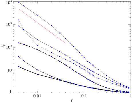
(a)    (b)

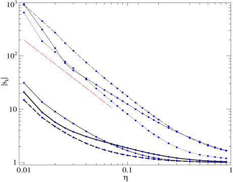
Figure 2: Maxima (thin lines) and r.m.s. values (bold lines) of $|{\bf s}_{k}|$: solid, dotted and dashed lines for $k=1,2,3$, respectively, for the full-spectrum (a) and non-helical (b) sample flows. Solid circles show the computed values. The long-dashed line shows, for reference, the inclination of the plot of the function $\eta^{-3/2}$ in the log-log coordinates of the respective figure.

Figure 2 indicates that in the limit $\eta\to 0$ the maxima of the neutral modes, ${\bf s}_{k}$, as well as their r.m.s. values apparently behave as $\eta^{-\kappa}$ for the exponent $\kappa=3/2$. This is a tentative conjecture, since the values of $\eta$ considered here are too high to confidently deduce the power-law behaviour from the numerical data. An analytical derivation of this estimate for $\kappa$ is desirable. We note that, when no small-scale dynamo operates, ${\bf s}_{k}$ can be obtained by integrating the magnetic induction equation (2) with the initial condition ${\bf h=e}_{k}$ up to infinite times. Such an evolutionary solution can be described for small molecular diffusivities by M.M. Vishik’s asymptotics [13]. It suggests that the maxima of ${\bf s}_{k}$ for $\eta\to\infty$ are at most order $\eta^{-3/2}$. However, it is difficult to prove the asymptotics along these lines, because that would require considering an interplay of the asymptotics in $\eta$ with the limit of infinitely large times.

We have checked that no small-scale dynamos operate for the magnetic molecular diffusivities employed in our computations; thus, the large-scale dynamos considered here are not overshadowed by (typically more efficient) small-scale dynamos.

(a)    (b)

Figure 3: Minimum magnetic eddy diffusivity $\eta_{\rm eddy}(\varphi)$ for six values of magnetic molecular diffusivity (coded by the dash length) for the full-spectrum (a) and non-helical (b) sample flows. Thin vertical lines are the asymptotes located at the points of the singularity.

(a)    (b)

Figure 4: Growth rate $\lambda_{2}^{+}(\varphi)$ for $\eta=0.02$ for the full-spectrum (a) and non-helical (b) sample flows. Graphs for $\theta$ (see (28)) step $\pi/8$ are coded by the dash length.

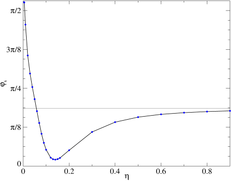
(a)    (b)

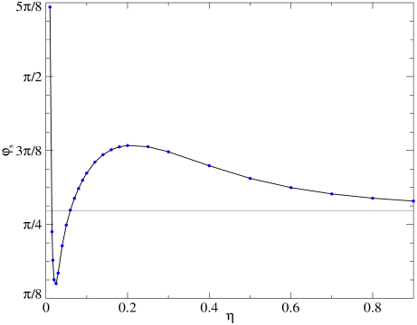
Figure 5: Location of the singularity (54) for the full-spectrum (a) and non-helical (b) sample flows. Solid circles show the computed values. Thin horizontal line: the limit location of the singularity (64) for $\eta\to\infty$.

Graphs of the computed minimum (over $\theta$ in (28)) magnetic eddy diffusivity $\eta_{\rm eddy}(\varphi)$ as a function of the azimuthal direction $\varphi$ of the wave vector $\bf q$ are shown in Fig. 3 for various values of magnetic molecular diffusivity $\eta$. (Recall that the minimum eddy diffusivity is a $\pi$-periodic function of $\varphi$, as we have demonstrated in section 4.6.) Two disjoint curves constituting a graph for a chosen $\eta$ and separated by the vertical asymptote are shown by dashed lines of the same dash length (depending on the $\eta$ value).

Dependencies of the growth rate $\lambda_{2}^{+}$ on $\varphi$ for latitudes $\theta=m\pi/8$ of the wave vector $\bf q$ directions (see (28)) are shown in Fig. 4 for $\eta=0.02$ and integer $m$ (as usual, negative growth rates are associated with decaying modes). Two disjoint curves related to the same $\theta$ are shown by dashed lines of the same dash length (different for different $\theta$). In view of the relation $\lambda_{2}^{+}(\theta,\varphi)=\lambda_{2}^{-}(\theta,\varphi+\pi)$ similar graphs for $\lambda_{2}^{-}$ are omitted. Since $\lambda_{2}^{+}$ is invariant under the mapping $\varphi\mapsto\varphi+\pi$, $\theta\mapsto\pi-\theta$ (see section 4.6), we show $\lambda_{2}^{+}$ only in a half-period interval $0\leq\varphi\leq\pi$. Therefore, a graph showing a certain value of $\lambda_{2}^{+}$ for $\varphi=\pi$ and some $\theta$ can be continuously extended for larger $\varphi$ by the graph of $\lambda_{2}^{+}$ for $\theta\to\pi-\theta$ starting at $\varphi=0$ at the same $\lambda_{2}^{+}$ value.

Both figures clearly illustrate the presence of the singularity (54) in the term $Q_{3}$ in the expressions for the growth rates (see (52)–(53)) and minimum eddy diffusivity, as well as the positive growth rates and negative eddy diffusivities in the vicinity of the singularity. The higher is $\eta$, the narrower gap between the continuous components separated by the vertical asymptotes is observed in Fig. 3 for graphs of the minimum eddy diffusivity, although this regularity is broken between $\eta=0.005$ and 0.02 for the full-spectrum flow in Fig. 3(a) and between $\eta=0.05$ and 0.1 for the non-helical flow in Fig. 3(b). Outside the gap around the asymptotes, $\eta_{\rm eddy}$ is very insensitive to the azimuthal direction $\varphi$.

The graphs for $\eta=0.02$ are notable: while magnetic eddy diffusivity is negative at the interval $0.898<\varphi<1.361$ around the singularity for the full-spectrum flow, it is negative at two longer intervals $0.202<\varphi<0.683$ around the singularity and $1.215<\varphi<2.616$ for the non-helical flow. This indicates that the importance of the kinetic helicity for kinematic magnetic field generation may be overestimated (see [9]).

The graph of the singular direction $\varphi_{\rm s}$ in Fig. 5 shows how the direction approaches the limit position (64) when molecular diffusivity $\eta$ indefinitely increases. Surprisingly, the high-diffusivity asymptotic regime sets in for the molecular diffusivities as low as 1/2.

6 Singular azimuthal directions

Here we focus on wave vectors $\bf q$ belonging to the plane of singular azimuthal directions $\varphi=\varphi_{\rm s}$ (54). An indefinite increase of the large-scale growth rate $\lambda_{2}$ suggests, as singularities often do in physics, that for these wave vectors the considered asymptotic expansions (6) break down. For $\varphi=\varphi_{\rm s}$, the matrix (32) in the l.h.s. of (31) is a $2\times 2$ Jordan cell. Accordingly [6, 11, 12], for the singular wave vectors we seek solutions to (4) in the form of power series in $\sqrt{\varepsilon}$:

$${\bf h(x,X})= \sum_{n=0}^{\infty}{\bf h}_{n}({\bf x,X})\varepsilon^{n/2},$$ (.1)

$$\lambda= \sum_{n=0}^{\infty}\lambda_{n}\varepsilon^{n/2}.$$ (.2)

Substituting (66) into (4) we obtain

$$\sum_{n=0}^{\infty}\left(\L{\bf h}_{n}+\eta(2(\nabla\cdot\nabla_{\bf X}){\bf h}_{n-2}+\nabla_{\bf X}^{2}{\bf h}_{n-4})+\nabla_{\bf X}\times({\bf v}\times{\bf h}_{n-2})-\sum_{m=0}^{n}\lambda_{n-m}{\bf h}_{m}\right)\varepsilon^{n/2}=0;$$ (67)

the solenoidality of the magnetic mode again implies relations (8) for all $n\geq 0$. The resultant hierarchy of equations can be solved in all orders and provides all terms in the series (66). They can be proved to be asymptotic series for the solution of the large-scale dynamo problem under consideration.

6.1 Order $\varepsilon^{0}$ equation

For $n=0$, (67) yields (9). As discussed in section 2.2, the suitable solution is $\lambda_{0}=0$, (10).

6.2 Order $\varepsilon^{1/2}$ equation

The next equation in the hierarchy (67) is then $\L{\bf h}_{1}=\lambda_{1}{\bf h}_{0}$. Averaging yields $0=\lambda_{1}\left\langle{\bf h}_{0}\right\rangle$, and for the same reasons the relevant choice is $\lambda_{1}=0$. Consequently,

$${\bf h}_{1}=\sum_{k=1}^{3}\left\langle{\bf h}_{1}\right\rangle_{k}{\bf s}_{k}.$$ (68)

6.3 Order $\varepsilon^{1}$ equation

For $n=2$, (67) implies

$$\L{\bf h}_{2}+2\eta(\nabla\cdot\nabla_{\bf X}){\bf h}_{0}+\nabla_{\bf X}\times({\bf v}\times{\bf h}_{0})=\lambda_{2}{\bf h}_{0}.$$ (69)

Substituting (10) and averaging, we find the solvability condition for this equation:

$$\nabla_{\bf X}\times(\bm{\mathfrak{A}}\left\langle{\bf h}_{0}\right\rangle)=\lambda_{2}\left\langle{\bf h}_{0}\right\rangle,$$ (70)

where $\bm{\mathfrak{A}}$ is the tensor of magnetic $\alpha$-effect (14). For $\lambda_{2}\neq 0$, (8) for $n=0$ is inevitably satisfied.

We suppose that large-scale magnetic modes are Fourier harmonics (27) for the wave vector $\bf q$ (28), where $\varphi=\varphi_{\rm s}$. The orthogonality of $\bf H$ and $\bf q$ justifies the use of (29)–(30) for reducing (70) to the eigenvalue problem

$${\rm i}\bm{\mathfrak{Z}}{\bf\Theta}=\lambda_{2}{\bf\Theta},\qquad{\bf\Theta}=\left[\begin{array}[]{l}\Theta_{\rm t}\\ \Theta_{\rm p}\end{array}\right],$$ (71)

where

$$\bm{\mathfrak{Z}}=\left[\begin{array}[]{cc}\mathfrak{z}&\mathfrak{z}^{\prime}\\ 0&\mathfrak{z}\end{array}\right],\qquad\mathfrak{z}=\mathfrak{A}^{2}_{3}\cos\theta,\qquad\mathfrak{z}^{\prime}=-(\mathfrak{A}^{3}_{1}\sin\varphi_{\rm s}+\mathfrak{A}^{1}_{2}\cos\varphi_{\rm s})\sin\,2\theta$$

(cf. (32)). Generically $\bm{\mathfrak{Z}}$ is essentially a $2\times 2$ Jordan cell, and we henceforth assume $\mathfrak{z}^{\prime}\neq 0$. Solutions to (71) and (69) are

$$\lambda_{2}={\rm i}\mathfrak{z},\qquad{\bf\Theta}=\left[\begin{array}[]{c}1\\ 0\end{array}\right],\qquad{\bf H}={\bf q}^{\rm t},$$ (72)

$${\bf h}_{2}=\sum_{k=1}^{3}\left(\left\langle{\bf h}_{2}\right\rangle_{k}{\bf s}_{k}+{\rm e}^{{\rm i}\bf q\cdot X}H_{k}\left(\lambda_{2}{\bm{\gamma}}_{k}+{\rm i}\sum_{m=1}^{3}q_{m}{\bf g}_{mk}\right)\right),$$ (73)

where ${\bm{\gamma}}_{k}({\bf x})$ and ${\bf g}_{mk}({\bf x})$ are small-scale zero-mean space-periodic solutions to auxiliary problems of types II (35) and II$\,{}^{\prime}$ (36).

6.4 Order $\varepsilon^{3/2}$ equation

For $n=3$, (67) yields

$$\L{\bf h}_{3}+2\eta(\nabla\cdot\nabla_{\bf X}){\bf h}_{1}+\nabla_{\bf X}\times({\bf v}\times{\bf h}_{1})=\lambda_{3}{\bf h}_{0}+\lambda_{2}{\bf h}_{1}.$$ (74)

The solvability condition for this equation is obtained by substituting (68) and averaging:

$$\nabla_{\bf X}\times(\bm{\mathfrak{A}}\left\langle{\bf h}_{1}\right\rangle)=\lambda_{3}\left\langle{\bf h}_{0}\right\rangle+\lambda_{2}\left\langle{\bf h}_{1}\right\rangle.$$ (75)

For $\lambda_{3}\neq 0$, (8) for $n=1$ is also inevitably satisfied.

The inhomogeneous term $\lambda_{3}\left\langle{\bf h}_{0}\right\rangle$ in (75) is proportional to ${\rm e}^{{\rm i}\bf q\cdot X}$ (see (27)). Together with (8) for $n=1$, this implies

$$\left\langle{\bf h}_{1}\right\rangle={\bf H}_{1}{\rm e}^{{\rm i}\bf q\cdot X},\quad{\bf H}_{1}\cdot{\bf q}=0\qquad\Rightarrow\qquad{\bf H}_{1}=\Theta_{\rm t1}{\bf q}^{\rm t}+\Theta_{\rm p1}{\bf q}^{\rm p},$$

whereby (75) transforms into

$${\rm i}\bm{\mathfrak{Z}}{\bf\Theta}_{1}=\lambda_{3}{\bf\Theta}+\lambda_{2}{\bf\Theta}_{1},\qquad{\bf\Theta}_{1}=\left[\begin{array}[]{l}\Theta_{\rm t1}\\ \Theta_{\rm p1}\end{array}\right].$$ (76)

We impose a normalisation condition $\Theta_{\rm t1}=0$ (satisfied by multiplying the mode by a suitable linear function of $\epsilon$, without altering the mode). Equation (76) is then equivalent to

$$\lambda_{3}={\rm i}\mathfrak{z}^{\prime}\Theta_{\rm p1},$$ (77)

and (74) has a solution

$${\bf h}_{3}=\sum_{k=1}^{3}\left(\left\langle{\bf h}_{3}\right\rangle_{k}{\bf s}_{k}+{\rm e}^{{\rm i}\bf q\cdot X}\left((\lambda_{2}H_{1k}+\lambda_{3}H_{k}){\bm{\gamma}}_{k}+{\rm i}\sum_{m=1}^{3}q_{m}{\bf g}_{mk}\right)\right).$$

6.5 Order $\varepsilon^{2}$ equation

For $n=4$, we infer from (67) the equation

$$\L{\bf h}_{4}+2\eta(\nabla\cdot\nabla_{\bf X}){\bf h}_{2}+\eta\nabla_{\bf X}^{2}{\bf h}_{0}+\nabla_{\bf X}\times({\bf v}\times{\bf h}_{2})=\lambda_{4}{\bf h}_{0}+\lambda_{3}{\bf h}_{1}+\lambda_{2}{\bf h}_{2}.$$

Averaging, substituting (73) and recalling that $\left\langle{\bf h}_{0}\right\rangle$ and $\left\langle{\bf h}_{1}\right\rangle$ are Fourier harmonics, we obtain its solvability condition:

$$\nabla_{\bf X}\times(\bm{\mathfrak{A}}\left\langle{\bf h}_{2}\right\rangle)+{\rm i}{\rm e}^{{\rm i}\bf q\cdot X}{\bf q}\times\sum_{k=1}^{3}H_{k}\left(\lambda_{2}\widetilde{\bm{\mathfrak{D}}}_{k}+{\rm i}\sum_{m=1}^{3}q_{m}\bm{\mathfrak{D}}_{mk}\right)=\lambda_{2}\left\langle{\bf h}_{2}\right\rangle+{\rm e}^{{\rm i}\bf q\cdot X}(\lambda_{3}{\bf H}_{1}+(\lambda_{4}+\eta){\bf H})$$ (78)

(see (38)). Therefore,

$$\left\langle{\bf h}_{2}\right\rangle={\bf H}_{2}{\rm e}^{{\rm i}\bf q\cdot X},\qquad{\bf H}_{2}=\Theta_{\rm t2}{\bf q}^{\rm t}+\Theta_{\rm p2}{\bf q}^{\rm p},$$

where we can also assume the normalisation condition $\Theta_{\rm t2}=0$. We denote $\displaystyle{\bf\Theta}_{2}=\left[\begin{array}[]{l}\Theta_{\rm t2}\\ \Theta_{\rm p2}\end{array}\right]$.

Now (78) takes the form

$${\rm i}\bm{\mathfrak{Z}}{\bf\Theta}_{2}+{\rm i}\sum_{k=1}^{3}H_{k}\left(\lambda_{2}\left[\begin{array}[]{r}\widetilde{\bm{\mathfrak{D}}}_{k}\cdot{\bf q}^{\rm p}\\ -\widetilde{\bm{\mathfrak{D}}}_{k}\cdot{\bf q}^{\rm t}\\ \end{array}\right]+{\rm i}\sum_{m=1}^{3}q_{m}\left[\begin{array}[]{r}\bm{\mathfrak{D}}_{mk}\cdot{\bf q}^{\rm p}\\ -\bm{\mathfrak{D}}_{mk}\cdot{\bf q}^{\rm t}\\ \end{array}\right]\right)=\lambda_{2}{\bf\Theta}_{2}+\lambda_{3}{\bf\Theta}_{1}+(\lambda_{4}+\eta){\bf\Theta}.$$

By (72) and (77), the second component of this equation reduces to

$$-{\rm i}\sum_{k=1}^{3}q^{\rm t}_{k}\left(\mathfrak{z}(\widetilde{\bm{\mathfrak{D}}}_{k}\cdot{\bf q}^{\rm t})+\sum_{m=1}^{3}q_{m}(\bm{\mathfrak{D}}_{mk}\cdot{\bf q}^{\rm t})\right)=\mathfrak{z}^{\prime}\Theta_{p1}^{2},$$

wherefrom we determine $\Theta_{p1}$ and $\lambda_{3}$. In view of the symmetry properties (48) of the tensor $\widetilde{\bm{\mathfrak{D}}}$, its contribution cancels out; using (51), we finally find

$$\lambda_{3}= \pm(1+i)\left({\mathfrak{z}^{\prime}\over 2}\sin\theta\left(\mathfrak{D}^{3}_{23}\cos^{3}\varphi_{\rm s}+(\mathfrak{D}^{3}_{33}-2\mathfrak{D}^{2}_{23})\cos^{2}\varphi_{\rm s}\sin\varphi_{\rm s}\right.\right.$$ (79)

$$\left.\left.+\,(\mathfrak{D}^{2}_{22}-2\mathfrak{D}^{3}_{32})\cos\varphi_{\rm s}\sin^{2}\varphi_{\rm s}+\mathfrak{D}^{2}_{32}\sin^{3}\varphi_{\rm s}\right)\vphantom{\mathfrak{z}^{\prime}\over 2}\!\right)\!^{1/2}\!.$$

While the leading term (with the coefficient $\lambda_{2}$ (72)) in the expansion (.2) of the eigenvalue is imaginary (i.e., the $\alpha$-effect remains oscillogenic for the singular azimuthal directions $\varphi=\varphi_{\rm s}$ of the wave vector, the period of oscillations being order $\varepsilon$, as before), the next term (with the coefficient $\lambda_{3}$ (79)) has a positive non-zero real part (unless the expression under the square root vanishes). This manifests a large-scale dynamo operating on the time scale O($\varepsilon^{3/2}t$). The decrease of this order for the singular directions of the wave vector is compatible with the singular behaviour of the large-scale growth rate $\lambda_{2}$ (52) calculated for non-singular directions, for which the large-scale dynamo operates on a slower time scale O($\varepsilon^{2}t)$.

The maximum of the large-scale growth rate over $\theta$ is admitted when $|\cos\theta|=1/\sqrt{3}$,

$$\max_{\theta}{\rm Re}\lambda_{3}=\sqrt{2\left|\mathfrak{D}^{3}_{23}(\mathfrak{A}^{1}_{2})^{3}+(\mathfrak{D}^{3}_{33}-2\mathfrak{D}^{2}_{23})(\mathfrak{A}^{1}_{2})^{2}\mathfrak{A}^{3}_{1}+(\mathfrak{D}^{2}_{22}-2\mathfrak{D}^{3}_{32})\mathfrak{A}^{1}_{2}(\mathfrak{A}^{3}_{1})^{2}+\mathfrak{D}^{2}_{32}(\mathfrak{A}^{3}_{1})^{3}\right|\over 3\sqrt{3}\left((\mathfrak{A}^{3}_{1})^{2}+(\mathfrak{A}^{1}_{2})^{2}\right)}.$$ (80)

6.6 Numerical results

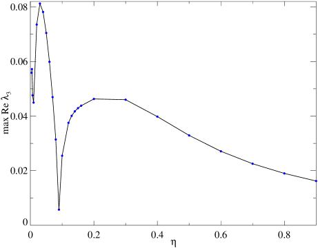
(a)    (b)

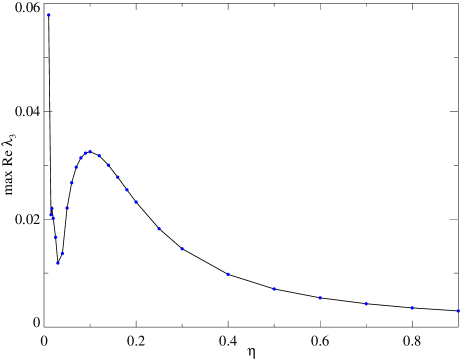
Figure 6: Maxima (80) of growth rates on the time scale O($\varepsilon^{3/2}t$) over wave vectors $\bf q$ belonging to the plane of singular azimuthal directions $\varphi=\varphi_{\rm s}$ for the full-spectrum (a) and non-helical (b) sample flows. Solid circles show the computed values.

Maxima (80) of growth rates on the time scale O($\varepsilon^{3/2}t$) over wave vectors $\bf q$ constituting the plane of singular azimuthal directions $\varphi=\varphi_{\rm s}$ have been computed for varying molecular diffusivity (see Fig. 6) for the same two sample flows as in section 5. We have done computations with the resolution of $128^{3}$ Fourier harmonics. For the smallest values of $\eta$ (0.004, 0.005 and 0.01 for the full-spectrum flow, Fig. 6(a), and 0.01 for the non-helical flow, Fig. 6(b)) the maxima have been verified in computations with the resolution of $256^{3}$ harmonics; they proved to coincide with the results of the $128^{3}$-harmonics runs in 4 significant digits.

The behaviour of the maximum growth rates for small molecular diffusivities becomes intermittent. Near the points, where the maximum vanishes, it exhibits a non-smooth (albeit continuous) behaviour, having in, agreement with (80), square-root-like cusps (although it is not sufficiently well resolved at the scale of Fig. 6). Such points are detected numerically as points, where there is a change of the sign of the cubic expression, whose absolute value is taken in the numerator in (80), and they have been evaluated by interpolation. For the non-helical flow, the growth of $\max_{\theta}{\rm Re}\lambda_{3}$ for decreasing $\eta$ is a consequence of the onset of the small-scale dynamo action; the maximum tends to infinity, when the critical molecular diffusivity for the onset of generation is approached. The mathematical reasons for such a behaviour are the same as the infinite decrease of magnetic eddy diffusivity (obtained by developing the conventional expansions (6)), when the dominant eigenvalue of the small-scale magnetic induction operator vanishes (see [15]) and solutions to auxiliary problems become large in magnitude.

We have observed in section 5 that the non-helical flow is more spatially intermittent than the full-spectrum one, suggesting that the former flow is a better dynamo than the latter one. However, examination of Fig. 6 reveals that the maximum growth rates (80) for the full-spectrum flow are higher than those for the non-helical one, except for when the critical molecular diffusivity for the onset of generation by the non-helical flow is approached (and outside a small interval in the vicinity of the zero maximum growth rate for the full-spectrum flow).

7 Concluding remarks

We have presented a two-scale dynamo sustained by the simultaneous action of the two most important large-scale mechanisms: the magnetic $\alpha$-effect and negative eddy diffusivity. (Interaction of the two mechanisms has somewhat amplified the entanglement of algebra involved in application of the homogenisation techniques. For instance, while auxiliary problems of type II (35) coincide with those encountered in the standard case of emergence of the phenomenon of magnetic eddy diffusivity when the magnetic $\alpha$-effect is absent (see Chapter 3 in [15]), auxiliary problems of type II$\hskip 1.0pt{}^{\prime}$ (36) have no analogues.) The influence of the $\alpha$-effect on generation of large-scale field is intricate. By virtue of (41), the growth rates $\lambda_{2}^{\pm}$ depend on the entries of the $\alpha$-effect tensor in two ways: via the first term, $\lambda_{1}^{\pm}$, in the expansion of the eigenvalue $\lambda$, and via the dependence of the ratios of components of vectors (.7) and (.6) on the ratio $\mathfrak{A}^{3}_{1}/\mathfrak{A}^{1}_{2}$. Not surprisingly, both the $\alpha$-effect and eddy diffusivity have nothing in common with the total kinetic helicity $\int{\bf v}\cdot(\nabla\times\bf v){\rm d}\bf x$; this becomes especially transparent when considering the large $\eta$ limit (see (59)–(61)); a heuristic argument explaining this in terms of the flow complexity and various topological properties of knottedness of vorticity lines was put forward in [9].

The dynamo operates as follows. The $\alpha$-effect creates a large-scale order $\varepsilon^{0}$ mean field $\left\langle{\bf h}_{0}\right\rangle$ (see (13)), oscillating in time on the time scale O$(\varepsilon^{-1})$, that neither grows, nor decays on this time scale. This mean field is accompanied by an O(1) suite field $\{{\bf h}_{0}\}$ fluctuating in space (see (10)), from which the small-scale flow creates an O$(\varepsilon)$ fluctuating field $\{{\bf h}_{1}\}$ (see (34)–(36)). Its interaction with the flow gives rise to an O$(\varepsilon)$ mean e.m.f. $\left\langle{\bf v}\times\{{\bf h}_{1}\}\right\rangle$ resulting in emergence of the magnetic eddy diffusivity, that can sustain the growth of the mean field $\left\langle{\bf h}_{0}\right\rangle$ on the O$(\varepsilon^{-2})$ time scale. Thus both the $\alpha$-effect and magnetic eddy diffusivity emerge due to the interaction of the small-scale flow with various components of the large-scale fluctuating magnetic field. The physics behind the two effects being basically the same, the difference between them is clearly observed at the mathematical level: the $\alpha$-effect acts on the O$(\varepsilon^{-1})$ time scale and it is described by the $\alpha$-effect operator

$${\bf h}\mapsto\nabla_{\bf X}\times(\bm{\mathfrak{A}}\bf h)$$

(cf. (26)) which is a differential operator of the first order; eddy diffusivity acts on the O$(\varepsilon^{-2})$ time scale, and the eddy diffusivity operator

$${\bf h}\mapsto\eta\nabla^{2}_{\bf X}{\bf h}+\nabla_{\bf X}\times\sum_{k=1}^{3}\left(\lambda_{1}h_{k}\widetilde{\bm{\mathfrak{D}}}_{k}+\sum_{m=1}^{3}\bm{\mathfrak{D}}_{mk}{\partial h_{k}\over\partial X_{m}}\right)$$

(cf. its symbol with the l.h.s. of (39)) is a differential operator of the second order. We encounter here a new $\alpha$-effect-like term $\lambda_{1}\nabla_{\bf X}\times\sum_{k=1}^{3}h_{k}\widetilde{\bm{\mathfrak{D}}}_{k}$, which does not appear in the eddy diffusivity operator for parity-invariant flows. (Since $\lambda_{1}$ (.1) is linear in $\bf q$, the contribution of this term is also quadratic in $\bf q$, and hence it can also be regarded as a second-order operator.)

Astrophysical dynamos are running at high kinetic, Re, and magnetic, Rm, Reynolds numbers such that the magnetic Prandtl numbers ${\rm P}_{m}={\rm Rm/Re}$ are typically very small (${\rm P}_{m}\ll 1$, e.g., in planetary interiors) or large (${\rm P}_{m}\gg 1$, e.g., in the interstellar medium). Such dynamos are problematic for theoretical analysis (see [10, 3, 8] for a discussion). An attractive feature of the two-scale dynamo under consideration, perhaps making it useful for astrophysical applications, is that (generically) it generates a mean field for all magnetic molecular diffusivities, i.e., for all ${\rm P}_{m}$ (although it is unclear what might coerce the small-scale turbulence to sustain the antisymmetry necessary for this dynamo). Apparently, the large-scale dynamo mechanism under consideration is not significantly hindered by the $\alpha$-quenching, since both the numerator and denominator in the singular function $Q_{3}(\varphi)$ (.4) — a constituent part of the growth rate $\lambda_{2}$ (52) — are linear and homogeneous in the entries of the $\alpha$-effect tensor. In the maximum growth rate (80) for singular azimuthal directions, the numerator and denominator are also both homogeneous in the entries of the $\alpha$-effect tensor, but their orders are different; as a result, $\max_{\theta}{\rm Re}\lambda_{3}\to 0$ when the $\alpha$-quenching occurs.

Our dynamo is characterised by a strong spatial focusing: interaction of the oscillogenic $\alpha$-effect and eddy diffusivity results in an upsurge of large-scale magnetic fields whose wave vectors belong to the “singular” plane $\varphi=\varphi_{\rm s}$ (normal to the plane of mirror antisymmetry of the flow). The respective mean fields are predominantly toroidal (i.e., predominantly parallel to the plane of mirror antisymmetry); they oscillate in the slow time O($\varepsilon t$) and have finite growth rates in the slow time O($\varepsilon^{3/2}t$). They are thus generated faster than fields for wave vectors outside the singular plane, whose growth rates are finite in the slow time O($\varepsilon^{2}t$).

The following questions remain open and will be addressed in future work.
$i$. The asymptotics that we have considered is in $\varepsilon\to 0$ followed by $\eta\to\infty$. It is of interest to consider other branches of solutions, in which $\varepsilon$ and $\eta$ vary simultaneously.
$ii$. Our small-scale flow is supposed to mimick the small-scale turbulent motion, making it is desirable to consider a more realistic case of flow, periodic in fast time (following the developments in chapter 4 of [15]).
$iii$. For a flow, antisymmetric in one Cartesian variable, that we have chosen to study, the $\alpha$-effect is oscillogenic for all magnetic molecular diffusivities, and also the eddy diffusivity tensors (38) possess various symmetry-type properties ((48) and (51)) which has given an opportunity to considerably simplify equations (e.g., expression for the growth rate $\lambda_{2}$ (52)). It was demonstrated in [9] that a flow features an oscillogenic $\alpha$-effect, whenever the symmetrised $\alpha$-effect tensor (whose entries are $(\mathfrak{A}^{m}_{k}+\mathfrak{A}^{k}_{m})/2$) has one zero eigenvalue and the two remaining eigenvalues have opposite signs (in our case the two non-zero eigenvalues of the symmetrised $\alpha$-effect tensor are $\pm\sqrt{(\mathfrak{A}^{1}_{3})^{2}+(\mathfrak{A}^{2}_{1})^{2}}$). An interesting question is to characterise the class of flows, for which the intermediate eigenvalue of the symmetrised $\alpha$-effect tensor is zero for all molecular diffusivities, and to derive for such flows the main term in the expansion of the growth rate Re $\lambda_{2}$.

References

References

- [1] Andrievsky A., Brandenburg A., Noullez A., Zheligovsky V. Negative magnetic eddy diffusivities from test-field method and multiscale stability theory. Astrophysical J. 811, 135 (2015) [arxiv.org/abs/1501.04465].
- [2] Arnold V.I., Zeldovich Ya.B., Ruzmaikin A.A., Sokoloff D.D. Steady magnetic field in a periodic flow. Dokl. Akad. Nauk SSSR, 266, 1357–1361 (1982).
- [3] Brandenburg A. Dissipation in dynamos at low and high magnetic Prandtl numbers. Astron. Nachr. 332, 725–731 (2011).
- [4] Chertovskih R., Zheligovsky V. Large-scale weakly nonlinear perturbations of convective magnetic dynamos in a rotating layer. Physica D, 313, 99–116 (2015) [arxiv.org/abs/1504.06856].
- [5] Gama S.M.A., Chertovskih R., Zheligovsky V. Computation of kinematic and magnetic -effect and eddy diffusivity tensors by Padé approximation. Fluids, submitted. (2019).
- [6] Kato T. Perturbation theory for linear operators. Springer, Berlin (1995), 2nd ed.
- [7] Liusternik L.A., Sobolev V.J. Elements of functional analysis. Frederick Ungar Publ., NY (1961).
- [8] Moffatt H.K. Helicity and celestial magnetism. Proc. R. Soc. A, 472, 20160183 (2016).
- [9] Rasskazov A., Chertovskih R., Zheligovsky V. Magnetic field generation by pointwise zero-helicity three-dimensional steady flow of an incompressible electrically conducting fluid. Phys. Rev. E, 97, 043201 (2018) [arxiv.org/abs/1708.08770].
- [10] Schekochihin A.A., Iskakov A.B., Cowley S.C., McWilliams J.C., Proctor M.R.E., Yousef T.A. Fluctuation dynamo and turbulent induction at low magnetic Prandtl numbers. New J. Physics, 9, 300 (2007).
- [11] Vishik M.M. Periodic dynamo. In: Mathematical methods in seismology and geodynamics (Computational seismology, iss. 19), 186–215. Eds. Keilis-Borok V.I., Levshin A.L. Nauka, Moscow, 1986. Engl. transl.: Computational seismology, 19, 176–209. Allerton Press, NY, 1987.
- [12] Vishik M.M. Periodic dynamo. II. In: Numerical modelling and analysis of geophysical processes (Computational seismology, iss. 20), 12–22. Eds. Keilis-Borok V.I., Levshin A.L. Nauka, Moscow, 1987. Engl. transl.: Computational seismology, 20, 10–21. Allerton Press, NY, 1988.
- [13] Vishik M.M. Magnetic field generation by the motion of a highly conducting fluid. Geophys. Astrophys. Fluid Dynamics, 48, 151–167 (1989).
- [14] Zheligovsky V. Numerical solution of the kinematic dynamo problem for Beltrami flows in a sphere. J. Scientific Computing, 8, 41–68 (1993).
- [15] Zheligovsky V.A. Large-scale perturbations of magnetohydrodynamic regimes: linear and weakly nonlinear stability theory. Lecture Notes in Physics, vol. 829, Springer-Verlag, Heidelberg, 2011.