An investigation of chaotic diffusion in a family of Hamiltonian mappings whose angles diverge in the limit of vanishingly action

Abstract

The chaotic diffusion for a family of Hamiltonian mappings whose angles diverge in the limit of vanishingly action is investigated by using the solution of the diffusion equation. The system is described by a two-dimensional mapping for the variables action, $I$, and angle, $\theta$ and controlled by two control parameters: (i) $\epsilon$, controlling the nonlinearity of the system, particularly a transition from integrable for $\epsilon=0$ to non-integrable for $\epsilon\neq 0$ and; (ii) $\gamma$ denoting the power of the action in the equation defining the angle. For $\epsilon\neq 0$ the phase space is mixed and chaos is present in the system leading to a finite diffusion in the action characterized by the solution of the diffusion equation. The analytical solution is then compared to the numerical simulations showing a remarkable agreement between the two procedures.

1 Introduction

The understanding of diffusive process has intrigued the humanity for long while. The reasons are vast and include since a very simple drop of colored ink in a jar with a fluid p1 , passing from other fields including medicine p2 such as how a given drug diffusing in the blood reaches a certain vital organ, biology/ecology p3 where pollen from a plant diffuses to reach another plant, environmental sciences with diffusion of pollution, no matter if gas (air) p4 with large impact in the earth, fluctuating solids in oceans traveling over the continents b1 , water percolation p5 in the ground transporting chemical reagents from pesticides to the water table and many other areas. In physics and considering its importance to the area, the subject is a so standard topic b2 ; b3 ; b4 which is delivered in undergrad courses around the world where basic properties of random walk are introduced together with other approaches.

In this paper we investigate the chaotic diffusion in a family of 2-D area preserving mappings described in the variables angle and action. The action is controlled by a parameter $\epsilon$ controlling also the nonlinearity of the system and particularly a transition from integrability to non integrability b5 . If $\epsilon=0$ the system is integrable and the phase space is regular. For $\epsilon\neq 0$, a mixed phase space is produced with the coexistence of regions with regularity marked by periodic islands and invariant spanning curves limiting the size of a chaotic sea, hence limiting the diffusion of chaotic particles. The variable angle is defined in such a way it diverges in the limit of vanishingly action p6 . The speed of the divergence is controlled by a parameter $\gamma>0$. Statistical properties of the chaotic sea have already been discussed under different approaches p7 ; p8 ; p9 ; p10 , mainly considering phenomenological techniques and numerical simulations. Scaling laws p11 leading to scaling invariance of the chaotic sea furnish an overall characterization of the universality of the problem. Our main goal in this paper is to describe the behavior of the statistical properties of the chaotic sea by using so far a solution of the diffusion equation b4 under specific boundary conditions. Our results are then compared to those already known in the literature p11 showing a remarkable agreement of the procedure.

This paper is organized as follows. In Sec. 2 we describe the Hamiltonian and the family of mappings showing applications for different systems. The scaling properties present in the system are highlighted also. Section 3 is devoted to discuss the solution of the diffusion equation and its implications to the dynamics for different time scalings as well as initial conditions. Our discussions and conclusions are presented in Sec. 4.

2 The mapping and its properties

The dynamics of an autonomous two degrees of freedom system can be described by a generic Hamiltonian b5 as $H(I_{1},I_{2},\theta_{1},\theta_{2})=H_{0}(I_{1},I_{2})+\epsilon H_{1}(I_{1},I_{2},\theta_{1},\theta_{2})$ where the term $H_{0}(I_{1},I_{2})$ gives the integrable part while $H_{1}(I_{1},I_{2},\theta_{1},\theta_{2})$ contributes to the non integrable part. The parameter $\epsilon$ controls a transition from integrability with $\epsilon=0$ to non-integrability for $\epsilon\neq 0$. Given the energy of the system is constant, the variable $I_{2}$ can be eliminated lasting three relevant variables. Using a Poincaré section in the plane $I_{1}\times\theta_{1}$ with $\theta_{2}$ constant the 3-D flow is reduced to an application in a 2-D mapping in the plane. A most generic mapping b5 that describes the dynamics is given by

$$\left\{\begin{array}[]{ll}I_{n+1}=I_{n}+\epsilon h(\theta_{n},I_{n+1})\\ \theta_{n+1}=[\theta_{n}+K(I_{n+1})+\epsilon p(\theta_{n},I_{n+1})]~{}~{}{\rm mod(2\pi)}\\ \end{array}\right.,$$ (1)

where $h(\theta_{n},I_{n+1})$, $K(I_{n+1})$ and $p(\theta_{n},I_{n+1})$ are nonlinear functions of their variables. The integer $n$ denotes the iterated of the mapping which preserves the area only if ${{\partial p(\theta_{n},I_{n+1})}\over{\partial\theta_{n}}}+{{\partial h(\theta_{n},I_{n+1})}\over{\partial I_{n+1}}}=0$.

Using $p(\theta_{n},I_{n+1})=0$ and $h(\theta_{n})=\sin(\theta_{n})$, different applications were already considered in the literature and to mention few of them

• $K(I_{n+1})=I_{n+1}$, describing the Chirikov-Taylor standard mapping JP31 ;

• $K(I_{n+1})=2/I_{n+1}$, gives the dynamics of a Fermi-Ulam model JP32 ; JP33 ;

• $K(I_{n+1})=\zeta I_{n+1}$, where $\zeta$ is a constant describes a bouncer model JP34 ;

• While for the case

  $$K(I_{n+1})=\left\{\begin{array}[]{ll}4\zeta^{2}(I_{n+1}-\sqrt{I_{n+1}^{2}-{{1}\over{\zeta^{2}}}})~{}~{}{\rm if}~{}~{}I_{n+1}>{{1}\over{\zeta}},\\ 4\zeta^{2}I_{n+1}~{}~{}{\rm if}~{}~{}I_{n+1}\leq{{1}\over{\zeta}}.\end{array}\right.$$

  with $\zeta$ constant recovers the hybrid Fermi-Ulam bouncer model JP35 ; EDL1 ; EDL2 ;

• $K(I_{n+1})=I_{n+1}+\zeta I_{n+1}^{2}$ recovers the logistic twist mapping JP30 .

Our goal in this paper is to investigate the dynamical properties for chaotic orbits considering a family of mappings described by $h(\theta_{n},I_{n+1})=\sin(\theta_{n})$ and $K=1/|I_{n+1}|^{\gamma}$ with $\gamma>0$ and $p(\theta_{n},I_{n+1})=0$, leading to

$$\left\{\begin{array}[]{ll}I_{n+1}=I_{n}+\epsilon\sin(\theta_{n})\\ \theta_{n+1}=[\theta_{n}+{{1}\over{|I_{n+1}|^{\gamma}}}]~{}~{}{\rm mod(2\pi)}\\ \end{array}\right..$$ (2)

We see that $\epsilon=0$ leads the phase space to be regular with $I$ constant while for $\epsilon\neq 0$ the regularity is partially destroyed being replaced by a mixed phase space including coexistence of chaos and regularity marked by periodic islands and invariant spanning curves limiting the size of the chaotic sea. Figure 1 shows a plot of the phase space of mapping (2) for the parameters $\gamma=1$ and: (a) $\epsilon=10^{-2}$ and (b) $\epsilon=10^{-3}$. The invariant spanning curves are shown in red (gray) color. Other values for the control parameters produce similar plots.

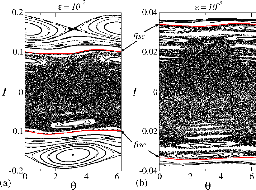
Figure 1: Plot of the phase space for mapping (2) considering $\gamma=1$ and: (a) $\epsilon=10^{-2}$; (b) $\epsilon=10^{-3}$. The invariant spanning curves, represented by fisc are shown in red (gray) color.

The chaotic sea is produced by absence of correlations between $\theta_{n+1}$ and $\theta_{n}$ in the limit of $I$ sufficiently small. For large values of the action correlations appear in $\theta$ producing regularity to the phase space consequently creating the invariant spanning curves, which play a major role in the dynamics p7 . The lowest one, denominated here as $I_{fisc}$, in either positive and negative sides work as a boundary prohibiting transport of particles through them. The index $fisc$ is a denotation to first invariant spanning curve. It is known b5 ; p8 that the position of the first invariant spanning curves from the mapping (2) can be described using a result imported from the Chirikov-Taylor standard map. Indeed in a transition from local to globally chaotic dynamics p11 , the position of the first invariant spanning curves are given by $I_{fisc}=\left[{{\gamma}\over{K_{ef}}}\right]^{{1}\over{\gamma+1}}\epsilon^{{1}\over{\gamma+1}}$, with a second order correction given by $\bigcirc^{2}\left({{\Delta I}\over{\tilde{I}}}\right)=-{{1}\over{2}}\left[{{K_{ef}}\over{\gamma}}\right]^{{1}\over{\gamma+1}}\epsilon^{{\gamma}\over{\gamma+1}}$. Here $K_{ef}$ denotes an effective parameter which describes locally the transition from local to globally chaotic dynamics. Starting the dynamics with very low action, a particle or an ensemble of non interacting particles, diffuses along the chaotic sea. The observable of interest is defined as $I_{rms}(n)=\sqrt{\overline{I^{2}}(n)}$, where

$$\overline{I^{2}}={{1}\over{M}}\sum_{i=1}^{M}\left[{{1}\over{n}}\sum_{j=1}^{n}I^{2}_{i,j}\right],$$ (3)

with $M$ corresponding to an average over an ensemble of $\theta\in[0,2\pi]$ and $n$ is the number of iterations of the mapping. The summation in $j$ is taken over the orbit while the summation in $i$ is realized over the ensemble of initial conditions. Indeed $I_{rms}$ behaves as follows. For short $n$ and $I_{0}\cong 0$, $I_{rms}$ starts to growth p11 with $n$ as $I_{rms}\propto(n\epsilon^{2})^{\beta}$ where $\beta=1/2$. This exponent is a confirmation that a chaotic particle diffuses as a random walk particle. For large enough $n$, $I_{rms}$ saturates due to the limits of the allowed regions to visit in the phase space. At such domain, $I_{rms}\propto\epsilon^{\alpha}$ where $\alpha$ is a critical exponent p7 . In fairness, $I_{sat}=\lim_{n\rightarrow\infty}I_{rms}$ must scale with the size of the chaotic sea. The limitations are $\pm I_{fisc}$, then $\alpha={{1}\over{1+\gamma}}$. The changeover from growth to the saturation is marked by $n_{x}\propto\epsilon^{z}$. The relevant scaling law already known p11 is $z={{\alpha}\over{\beta}}-2$, leading to $z=-{{2\gamma}\over{\gamma+1}}$.

It the initial action is no longer small enough but is still smaller than $I_{sat}$, the ensemble of particles diffuses as follows. Part of the ensemble increases action with probability $p$ and part of it decreases with probability $q=1-p$. Since there is no bias in the system, then $p=q$ and half of the ensemble increases/decreases. Eventually this symmetry is broken p9 and an additional scaling is observed. $I_{rms}$ stays in a plateau until a crossover time $n_{n}^{\prime}$ that scales with $n_{x}^{\prime}\propto{{I_{0}^{2}}\over{\epsilon^{2}}}$. If an ensemble of initial conditions is given above of the saturation and below of the first invariant spanning curve the scenario can be very complicated due to the existence of stickiness p12 . The relevant scaling transformations p8 ; p11 that lead all the curves of $I_{rms}$ obtained from different $\epsilon$ and $I_{0}$ to overlap each other are: (i) $I_{rms}\rightarrow I_{rms}/\epsilon^{\alpha}$; (ii) $n\rightarrow n/\epsilon^{z}$ and; (iii) $I_{0}^{\prime}=I_{0}\left({{\epsilon^{\prime}}\over{\epsilon}}\right)^{{1}\over{1+\gamma}}$.

3 Solution for the diffusion equation

The characteristics observed in the phase space, particularly in the chaotic dynamics, allow us to make a connection with diffusive problems. Firstly when an initial condition is given in the chaotic sea at the regime of low action, typically $I_{0}\sim 10^{-3}\epsilon$, the dynamics diffuses chaotically along the phase space passing near the islands and visiting regions close to the invariant spanning curves. Because the mapping is area preserving the transport of particles through such curves is not allowed. An immediate conclusion is that, once in the chaos, always in the chaos.

Whenever making a connection with statistical mechanics, a chaotic particle has probability $p>0$ of moving one side, say increasing the action, and $q=1-p>0$ of moving other side, decreasing the action, therefore resembling a motion of a random walk process. Due to the property of area preservation, a particle can not traverse the invariant spanning curves. They work as reflecting barriers. A diffusion equation b4 written for the variable action $I$ and the number of iterations $n$, denoting the time, is given by

$${{\partial P(I,n)}\over{\partial n}}=D{{\partial^{2}P(I,n)}\over{\partial I^{2}}},$$ (4)

where $D$ is the diffusion coefficient obtained from the relation $D={{(\overline{\Delta I})^{2}}\over{2}}=\bar{I^{2}}_{n+1}-\bar{I^{2}}_{n}={{\epsilon^{2}}\over{4}}$ and $P(I,n)$ gives the probability of observe a given action $I\in[-I_{fisc},+I_{fisc}]$ at a given time $n$. The boundary conditions for this problem are ${{\partial P}\over{\partial I}}\big{|}_{\pm I_{fisc}}=0$ implying no flux of particles through the invariant spanning curves.

There are many different ways of solving the equation (4). In our case we used a technique of separation of variables therefore writing $P(I,n)=X(I)N(n)$ where, as usual, $X(I)$ is a function that depends only on $I$ and $N(n)$ is another function that depends only on $n$. This technique transforms the original partial differential equation, first order in $n$ and second order in $I$ into two ordinary differential equations that must be solved separately. Such separation is allowed under the assumption that the variables $I$ and $n$ are independent of each other. We considered also that at a time $n=0$, all the initial particles were localized at $P(I,0)=\delta(I-I_{0})$ with $I_{0}\in[-I_{fisc},+I_{fisc}]$ and along the chaotic sea. $I_{0}\cong 0$ gives the maximal diffusion possible observed for $I_{rms}$. When $I_{0}\neq 0$ an additional scaling is observed in the dynamics p8 ; p11 .

Since the procedure is standard in many textbooks, see for example Ref. b4 , we report only the final solution

$$P[I(n)]={{1}\over{2I_{fisc}}}+{{1}\over{I_{fisc}}}\sum_{k=1}^{\infty}\cos\left[{{k\pi(I-I_{0})}\over{I_{fisc}}}\right]e^{-{{k^{2}\pi^{2}Dn}\over{I^{2}_{fisc}}}},$$ (5)

where $I_{0}$ defines the initial action along the chaotic sea, $n$ corresponds to the number of iterations of the mapping and $k$ comes from the boundary conditions and must be in the interval $k\in[1,\infty)$. In practical, the summation does not need to run to infinity. Because the exponentials decay with the square of $k$, few terms on $k$ are enough. We have used for safety in our numerical results $k=100$ but one can not see great differences of $k=100$ with the first order approximation $k=1$, which is indeed the leading term of the summation.

The knowledge of the probability function $P[I(n)]$ allows us to obtain different observables in the phase space. Since the phase space is symmetrical with respect to the action $I$, particularly the symmetry for $I$ inside of the range $I\in[-I_{fisc},+I_{fisc}]$, the most interesting observable to be studied is $\overline{I^{2}}(n)$ instead of $\overline{I}(n)$. It is obtained from direct integration of $\overline{I^{2}}(n)=\int_{-I_{fisc}}^{I_{fisc}}I^{2}P[I(n)]dI$, which leads to the following expression

$$\overline{I^{2}}(n)=I^{2}_{fisc}\left[{{1}\over{3}}+{{4}\over{\pi^{2}}}\sum_{k=1}^{\infty}{{(-1)^{k}}\over{k^{2}}}\cos\left({{k\pi I_{0}}\over{I_{fisc}}}\right)e^{-{{k^{2}\pi^{2}Dn}\over{I^{2}_{fisc}}}}\right].$$ (6)

To have a clear comparison of the results produced by Equation (6) we have to obtain the observable $I_{rms}(n)=\sqrt{\overline{I^{2}}(n)}$.

Since Equation (4) was solved to give the probability of finding an action $I$ already averaged over an ensemble at an instant $n$, then we have to take an average on $n$ in the Equation (6) to make comparisons feasible. We notice the sum in $n$ for Equation (6) affects only the exponential term. The summation over the exponential terms gives a perfect geometrical series which converges well. Averaging then Equation (6) over $n$ we end up with the following expression

$$I_{rms} (n)=I_{fisc}$$

$$\times \sqrt{{{1}\over{3}}+{{4}\over{\pi^{2}}}\sum_{k=1}^{\infty}{{(-1)^{k}}\over{k^{2}}}\cos\left({{k\pi I_{0}}\over{I_{fisc}}}\right)e^{-{{k^{2}\pi^{2}D}\over{I^{2}_{fisc}}}}\left[{{1}\over{n}}\left({{(1-e^{-{{k^{2}\pi^{2}Dn}\over{I^{2}_{fisc}}}})}\over{(1-e^{-{{k^{2}\pi^{2}D}\over{I^{2}_{fisc}}}})}}\right)\right]},$$

when $n$ must run from $n=1,2\ldots\infty$. Figure 2

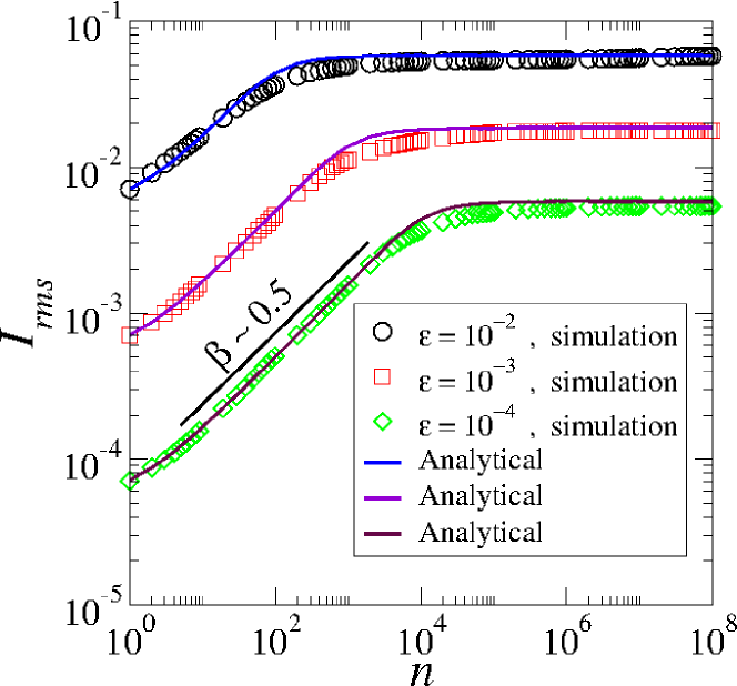
Figure 2: Plot of $I_{rms}~{}vs.~{}n$ for different control parameters as labeled in the figure. Symbols are used for numerical simulation while continuous line represent the analytical solution given by equation (3).

shows a plot of $I_{rms}(n)~{}vs.~{}n$ for $\gamma=1$ and three control parameters namely: $\epsilon=10^{-2}$, $\epsilon=10^{-3}$ and $\epsilon=10^{-4}$. We used $I_{0}=10^{-3}\epsilon$ as initial action leading to a situation of maximizing the diffusion for $I_{rms}$. Symbols represent the numerical simulations while continuous line are the theoretical result. The error bar produced by the simulations for an ensemble of $M=5\times 10^{3}$ different initial conditions is smaller then the symbols size. We see that the curve starts to growth with an exponent $\beta$ as a function of $n$ and suddenly it bends towards a regime of saturation for large enough $n$. The changeover from growth to the saturation is defined by a crossover $n_{x}$. The slope of growth is marked by an exponent $\beta\cong 1/2$ as theoretically foreseen in Ref. p11 . For large enough $n$, the saturation of the curves represents the influence of the invariant spanning curves in the phase space therefore limiting the diffusion in the action. For the regime of $n\rightarrow\infty$, $\lim_{n\rightarrow\infty}I_{rms}={{I_{fisc}}\over{\sqrt{3}}}\cong{{I_{fisc}}\over{1.732\ldots}}$. A naive estimation of $I_{rms}$ in Ref. p11 led to $I_{sat}\sim I_{fisc}/1.8$, therefore furnishing a good agreement between the theoretical and numerical results.

Let us now discuss the leading term of equation (3). Whenever considering a first order approximation we chose $k=1$ and two different cases: (i) $I_{0}\cong 0$ and (ii) $0<I_{0}<I_{fisc}/\sqrt{(}3)$. We start first with case (i). The nonlinear function used in equation (3) can be expanded in Taylor series until first order as

$$\cos\left({{\pi I_{0}}\over{I_{fisc}}}\right) \cong \left[1-{{1}\over{2}}\left({{\pi I_{0}}\over{I_{fisc}}}\right)^{2}\right],$$ (8)

$$e^{-{{\pi^{2}D}\over{I^{2}_{fisc}}}} \cong 1-{{\pi^{2}D}\over{I^{2}_{fisc}}},$$ (9)

$$1-e^{-{{\pi^{2}D}\over{I^{2}_{fisc}}}} \cong {{\pi^{2}D}\over{I^{2}_{fisc}}}.$$ (10)

Because of the presence of the factor ${{1}\over{n}}$ in equation (3), the expression for the exponential depending on $n$ must be expanded to the second order, then

$$1-e^{-{{\pi^{2}Dn}\over{I^{2}_{fisc}}}}\cong{{\pi^{2}D}\over{I^{2}_{fisc}}}-{{\pi^{4}D^{2}n^{2}}\over{2I^{4}_{fisc}}}.$$ (11)

Substituting these terms in equation (3), grouping them properly and after consider that $D={{\epsilon^{2}}\over{4}}$ we obtain

$$I_{rms}(n)\cong\sqrt{\left({{1}\over{3}}-{{4}\over{\pi^{2}}}\right)\epsilon^{{1}\over{1+\gamma}}+{{\epsilon^{2}n}\over{2}}},$$ (12)

and that the variation in $n$ leads to $I_{rms}\propto\sqrt{{\epsilon^{2}n}\over{2}}$. This result confirms the exponent $\beta=1/2$ as well as the transformation ad-hoc $n\rightarrow n\epsilon^{2}$ used in Ref. p11 . When such a regime of growth intersects $I_{sat}$, the crossover emerges, hence $\sqrt{{\epsilon^{2}n_{x}}\over{2}}={{\epsilon^{{1}\over{1+\gamma}}}\over{\sqrt{3}}}$, leading to

$$n_{x}\propto{{2}\over{3}}\epsilon^{-{{2\gamma}\over{1+\gamma}}},$$ (13)

therefore $z=-{{2\gamma}\over{1+\gamma}}$.

Let us now discuss the case (ii) with $0<I_{0}<{{I_{fisc}}\over{\sqrt{3}}}$. Figure 3(a)

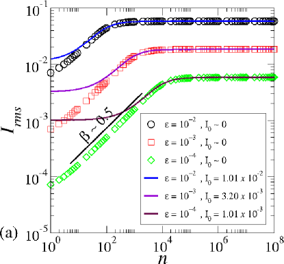
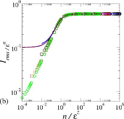
Figure 3: (a) Plot of $I_{rms}~{}vs.~{}n$ for different control parameters as well as different values of $I_{0}$, as labeled in the figure. Symbols are used for $I_{0}\cong 0$ while continuous line represent $0<I_{0}<{{I_{fisc}}\over{\sqrt{3}}}$. (b) Overlap of the curves shown in (a) onto an universal plot after the scaling transformations.

shows a plot of $I_{rms}~{}vs.~{}n$ for different values of $\epsilon$ as well as different initial conditions, as labeled in the figure. The plateaus for short $n$ are evident, confirming the additional scaling. The initial conditions generating the plateaus were chosen as $I_{0}^{\prime}=I_{0}\left({{\epsilon^{\prime}}\over{\epsilon}}\right)^{{1}\over{1+\gamma}}$. Figure 3(b) shows the overlap of the curves depicted in (a) onto an universal plot, where curves with $0<I_{0}<{{I_{fisc}}\over{\sqrt{3}}}$ overlap between them for short $n$, then they join the regime of growth and finally bend, all together, towards a regime of saturation for large enough $n$.

Keeping now the approximation with $I_{0}\neq 0$ from equation (8), substituting it into equation (3), the first crossover is given when

$${{1}\over{3}}-{{4}\over{\pi^{2}}}\left(1-{{1}\over{2}}\left({{\pi I_{0}}\over{I_{fisc}}}\right)^{2}\right)\left(1-{{\pi^{2}Dn_{x}^{\prime}}\over{2I^{2}_{fisc}}}\right)=1.$$ (14)

Doing the proper algebra and considering only the leading term for the Taylor expansion in $I_{0}/I_{fisc}$ we end up with

$$n_{x}^{\prime}\propto{{\pi^{2}}\over{3}}{{I_{0}^{2}}\over{\epsilon^{2}}},$$ (15)

as obtained in Ref. p8 for $\gamma=1$.

Let us now comment on the possible influence of the stickiness in the diffusion along the chaotic sea. As discussed in Ref. p12 and also in references therein, the survival probability corresponds to the probability a particle survive along the chaotic dynamics inside a given domain without escaping such region. The survival probability, is obtained from the integration of the escape frequency histogram written as

$$\rho(I_{n})={{1}\over{N}}\sum_{i=1}^{N}N_{rec}(n),$$ (16)

where $N$ denotes the number of different initial conditions, $n$ is the iteration number and $I$ is the action. We consider in our simulations to obtain $\rho$ an ensemble size of $N=10^{9}$ different initial conditions with $I_{0}=10^{-3}\epsilon$ and $\theta_{0}$ uniformly distributed in the interval $[0,2\pi]$ and a limiting number of iteration of $n=5\times 10^{5}$. We show the results for $\epsilon=10^{-3}$ although similar results would be obtained for other values of $\epsilon$. We define a given position along the action axis inside of the chaotic sea identified as $-I_{fisc}<h<I_{fisc}$. Starting the dynamics the orbit can evolve in the chaotic sea. If the particle reaches $h$ we consider it escaped such region. We determine then the number of iterations spent until that time and started a different initial condition. This procedure is repeated until the ensemble of $10^{9}$ different phases is completely exhausted. If the phase space shows only chaos the survival probability is described by an exponential decay p12 while the existence of islands lead to local trapping, changing the exponential decay to a slower decay that might be a stretched exponential or a power law. Figure 4(a) shows

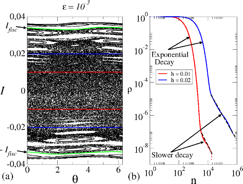
Figure 4: (a) Plot of the phase space for mapping (2) considering $\gamma=1$ and $\epsilon=10^{-3}$; (b) the behavior of the survival probability for orbits in the chaotic sea of (a) surviving the regions $h\in[-0.01,0.01]$ and $h\in[-0.02,0.02]$.

a plot of the phase space for the parameter $\epsilon=10^{-3}$ and two regions delimited by the values $h=0.01$ (inside the red lines) and $h=0.02$ (inside the blue lines). The two curves shown in Fig. 4(b) correspond to the survival probability obtained for chaotic orbits started in the chaotic sea with $I_{0}=10^{-3}\epsilon$ and different initial phases. We see they decay to start with at an exponential shape and eventually a small fraction of them gets stick near periodic islands for a while. The slower than exponential decay is a confirmation of the local and temporally confinement. The red curve decaying first corresponds to the region of $-0.01<h<0.01$. The periodic regions, not visible at the scale of the figure, influence only a portion of about $100$ particles from an ensemble of $10^{9}$, therefore statistically unidentifiable. The blue curve corresponds to a region of $-0.02<h<0.02$ and decays latter that the red curve. The stickiness affects about $50,000$ particles from an ensemble of $10^{9}$, therefore also very difficult to be detected in the simulations. Even though the stickiness is present at the domain investigated, its influence does not change the main results obtained.

4 Discussions and conclusions

We have investigated some scaling properties for a family of two-dimensional, nonlinear and area preserving maps whose angle diverges in the limit of vanishingly action. The parameter $\epsilon$ controls the nonlinearity of the problem and also a transition from integrable to non-integrable. The relevant scalings from the first momenta of the variable action is obtained numerically as well as by solution of the diffusion equation. For short $n$ and starting with low initial action, the behavior of $I_{rms}$ grows as $n$ with a power of $\beta=1/2$. Such exponent emerged naturally from the analytical solution. The regime of saturation scales with $\epsilon^{\alpha}$. Our finding for the regime of $\lim_{n\rightarrow\infty}$ yielded $I_{sat}\propto\epsilon^{{1}\over{(1+\gamma)}}$ in total agreement with the results already known in the literature p7 ; p8 ; p9 ; p11 . Our results obtained from the solution of the diffusion equation for the regime of initial action $0<I_{0}<{{I_{fisc}}\over{\sqrt{3}}}$ produces the additional plateau with the same relevant scaling as observed in Refs. p8 ; p11 . The additional scaling is related to the symmetry of the probability distribution function p9 and the break of symmetry produces the new crossover time.

The formalism presented in this paper has shown to be very robust and reliable to investigate chaotic transport. Future applications could involve study of diffusion of energy in time-dependent billiards, the scalings observed in the transition from limited to unlimited energy in a domain ranging from non-conservative to conservative system and many other applications. A problem that is still open and deserves much investigation relates to the dynamical trapping also called as stickiness for regions of the phase space near the invariant spanning curves. When a particle passes enough close such regions, they may stay trapped for a while - eventually long - until escape and run its own dynamics. During the trapping, the normal diffusion is mostly replaced by anomalous diffusion. This transition is not clear yet and deserves more investigation.

- (1) S. Lee, H-Y. Lee, I-F. Lee, C-Y Tseng, Ink diffusion in water, European Journal of Physics, 25, 331 (2004)
- (2) K. Murase, S. Tanada, H. Mogami, M. Kawamura, M. Miyagawa, M. Yamada, H. Higashiro, A. Lio, K. Hamamoto, Validity of microsphere model in cerebral blood flow measurement using N-isopropyl-p-(I-123) iodoamphetamine, Medical Physics, 19, 70, (1990)
- (3) W. F. Morris, Predicting the Consequence of Plant Spacing and Biased Movement for Pollen Dispersal by Honey Bees, Ecology, 74, 493, (1993).
- (4) D. Popp, International innovation and diffusion of air pollution control technologies: the effects of NOX and SO2 regulation in the US, Japan, and Germany, Journal of Environmental Economics and Management, 51, 46, (2006).
- (5) R. V. Ozmidov, Diffusion of contaminants in the ocean, Springer, (1990)
- (6) C. Hagedorn, E. L. Mc Coy, T. M. Rahe. The Potential for Ground Water Contamination from Septic Effluents, J. Environ. Qual., 10, 1, (1981)
- (7) R. K. Patria, Statistical Mechanics, Elsevier (2008)
- (8) F. Reif, Fundamentals of statistical and thermal physics, New York: McGraw-Hill, (1965)
- (9) V. Balakrishnan, Elements of nonequilibrium statistical mechanics, Ane Books India, New Delhi (2008)
- (10) A. J. Lichtenberg, M. A. Lieberman, Regular and chaotic dynamics (Appl. Math. Sci.) 38, Springer Verlag, New York, (1992)
- (11) J. A. de Oliveira, R. A. Bizão, E. D. Leonel, Finding critical exponents for two-dimensional Hamiltonian maps, Phys. Rev. E, 81, 046212 (2010)
- (12) E. D. Leonel, J. A. de Oliveira, F. Saif, Critical exponents for a transition from integrability to non-integrability via localization of invariant tori in the Hamiltonian system, J. Phys. A, 44, 302001 (2011)
- (13) E. D. Leonel, P. V. E. McClintock, J. K. L. da Silva, Fermi-Ulam accelerator model under scaling analysis, Physical Review Letters, 93, 014101 (2004)
- (14) D. F. M. Oliveira, M. R. Silva, E. D. Leonel, A symmetry break in energy distribution and a biased random walk behavior causing unlimited diffusion in a two dimensional mapping, Physica A, 436, 909, (2015)
- (15) J. A. Oliveira, C. P. Dettmann, D. R. Costa, E. D. Leonel, Scaling invariance of the diffusion coefficient in a family of two-dimensional Hamiltonian mappings, Physical Review E, 87, 062904 (2015)
- (16) E. D. Leonel, J. Penalva, R. M. N. Teixeira, R. N. Costa Filho, M. R. Silva, J. A. Oliveira, A dynamical phase transition for a family of Hamiltonian mappings: A phenomenological investigation to obtain the critical exponents, Physics Letters A, 379, 1808 (2015).
- (17) B. V. Chirikov, A universal instability of many-dimensional oscillator systems, 52, 263 (1979)
- (18) M. A. Lieberman, J. A. Lichtenberg, Stochastic and adiabatic behavior of particles accelerated by periodic forces, Phys. Rev. A, 5, 1852 (1971)
- (19) J. K. L. da Silva, D. G. Ladeira, E. D. Leonel, P. V. E. McClintock, S. O. Kamphorst, Scaling properties of the Fermi-Ulam accelerator model, Braz. J. Phys., 36, 700 (2006)
- (20) L. D. Pustylnikov, Stable and oscillating motions in non-autonomous dynamical systems, Trans. Moscow Math. Soc., 2, 1 (1978)
- (21) E. D. Leonel, P. V. E. McClintock, A hybrid Fermi-Ulam bouncer model, J. Phys. A, 38, 823 (2005)
- (22) D. G. Ladeira, E. D. Leonel, Dynamical properties of a dissipative hybrid Fermi-Ulam-bouncer model, Chaos, 17, 013119 (2007)
- (23) D. F. M. Oliveira, R. A. Bizão, E. D. Leonel, Scaling properties of a hybrid Fermi-Ulam-bouncer model, Mathematical Problems in Engineering, Volume 2009, Article ID 213857, (2009)
- (24) J. E. Howard, J. Humphreys, Nonmonotonic twist maps, Physica D, 80, 256, (1995)
- (25) A. L. P. Livorati et al, Investigation of stickiness influence in the anomalous transport and diffusion for a non-dissipative Fermi-Ulam model, Commun Nonlinear Sci Numer Simulat, 55, 225 (2018)