Details of the disorder-induced transition between $s_{\pm}$ and $s_{++}$ states in two-band model for Fe-based superconductors

Abstract

Irradiation of superconductors with different particles is one of many ways to investigate effects of disorder. Here we study the disorder-induced transition between $s_{\pm}$ and $s_{++}$ states in two-band model for Fe-based superconductors with nonmagnetic impurities. Specifically, the important question of whether the superconducting gaps during the transition change smoothly or steeply? We show that the behavior can be of either type and is controlled by the ratio of intra- and interband impurity scattering and a parameter $\sigma$ that represents a scattering strength and changes from zero (Born approximation) to one (unitary limit). For the pure interband scattering potential and $\sigma\lesssim 0.11$, the $s_{\pm}\to s_{++}$ transition is accompanied by the steep behavior of gaps, while for larger values of $\sigma$, gaps change smoothly. The steep behavior of the gaps occurs at low temperatures, $T<0.1T_{c0}$, otherwise it is smooth. The critical temperature $T_{c}$ is always a smooth function of the scattering rate in spite of the steep changes in the behavior of the gaps.

Keywords: unconventional superconductors, iron pnictides, iron chalcogenides, impurity scattering

1 Introduction

Iron-based materials reveal intriguing behavior in a number of physical properties. This includes unconventional superconductivity [1, 2, 3, 4, 5, 6], transport coefficients and Raman spectra [7, 8, 9, 10], magnetic and nematic states [11, 12, 13, 14], and electronic band structure [15, 16, 17, 18, 19]. First one is of a special interest because transition temperature to the superconducting state ($T_{c}$) is as high as 58 K in bulk materials [20] and up to 110 K in a monolayer FeSe [21, 22, 23, 24, 25].

Except for the extreme hole and electron dopings, the Fermi surface of Fe-based materials consists of two or three hole sheets around the $\Gamma=(0,0)$ point and two electron sheets around the $M=(\pi,\pi)$ point of the two-Fe Brillouin zone. Scattering between them with the large wave vector results in the enhanced antiferromagnetic fluctuations, which promote the $s_{\pm}$ type of the superconducting order parameter that change sign between electron and hole pockets [1, 3, 26]. On the other hand, bands near the Fermi level have mixed orbital content and orbital fluctuations enhanced either by vertex corrections or the electron-phonon interaction may lead to the sign-preserving $s_{++}$ state [27, 28, 29, 30, 31]. However, most experimental data including observation of a spin-resonance peak in inelastic neutron scattering, the quasiparticle interference in tunneling experiments, and NMR spin-lattice relaxation rate are in favor of the $s_{\pm}$ scenario [3, 6].

Superconducting states with different symmetries and structures of order parameters act differently being subject to the disorder [32]. That is, in the single-band $s$-wave superconductor, nonmagnetic impurities do not suppress $T_{c}$ according to the Anderson’s theorem [33], while the magnetic disorder cause the $T_{c}$ suppression with the rate following the Abrikosov-Gor’kov theory [34]. In the unconventional superconductors, suppression of the critical temperature as a function of a parameter $\Gamma$ characterizing impurity scattering may follow a quite complicated law. Several experiments on iron-based materials show that the $T_{c}$ suppression is much weaker than expected in the framework of the Abrikosov-Gor’kov theory for both nonmagnetic [35, 36, 37, 38, 39, 40, 41] and magnetic disorder [36, 42, 43, 44, 45]. Many theoretical studies revealed the importance of the multiband effects in this matter, see Refs. [46, 47, 48, 49, 50, 51, 52, 53]. One of the conclusions was that the system having the $s_{\pm}$ state in the clean case may preserve a finite $T_{c}$ in the presence of nonmagnetic disorder due to the transition to the $s_{++}$ state. It was obtained both in the strong-coupling $\mathcal{T}$-matrix approximation [50] and via a numerical solution of the Bogoliubov-de Gennes equations [54, 55].

Topology of the Fermi surface in Fe-based materials makes it sensible to use a two-band model as a compromise between simplicity and possibility to capture some essential physics. Previously, we have studied the $s_{\pm}\to s_{++}$ transition in such a model and shown that the transition can take place only in systems with the sizeable effective intraband pairing interaction [50]. Physical reason for the transition is quite transparent, namely, if one of the two competing superconducting interactions leads to the state robust against impurity scattering, then although it was subdominating in the clean limit, it should become dominating while the other state is destroyed by the impurity scattering [32]. Here we focus on the details of the $s_{\pm}\to s_{++}$ transition. In particular, we are interested in the behavior of the superconducting gaps across the transition. We show that in the case of a weak scattering (including the Born limit) at low temperatures, the gaps behaves steeply, while in all other cases they change smoothly across the transition.

2 Model

Hamiltonian of the two-band model can be written in the following form:

$$H=\sum\limits_{\mathbf{k},\alpha,\sigma}\xi_{\mathbf{k}\alpha}c_{\mathbf{k}\alpha\sigma}^{{\dagger}}c_{\mathbf{k}\alpha\sigma}+\sum\limits_{\mathbf{R}_{i},\sigma,\alpha,\beta}\mathcal{U}_{\mathbf{R}_{i}}^{\alpha\beta}c_{\mathbf{R}_{i}\alpha\sigma}^{{\dagger}}c_{\mathbf{R}_{i}\beta\sigma}+H_{sc},$$ (1)

where $c_{\mathbf{k}\alpha\sigma}$ is the annihilation operator of the electron with a momentum $\mathbf{k}$, spin $\sigma$, and a band index $\alpha$ that equals to $a$ (first band) or $b$ (second band), $\xi_{\mathbf{k}\alpha}$ is the electron dispersion that, for simplicity, we treat as a linearized one near the Fermi level, $\xi_{\mathbf{k}\alpha}=\mathbf{v}_{F\alpha}(\mathbf{k}-\mathbf{k}_{F\alpha})$, with $\mathbf{v}_{F\alpha}$ and $\mathbf{k}_{F\alpha}$ being the Fermi velocity and the Fermi momentum of the band $\alpha$, respectively. Presence of disorder is described by the nonmagnetic impurity scattering potential $\mathcal{U}$ at sites $\mathbf{R}_{i}$.

Superconductivity occurs in our system due to the interaction $H_{sc}$ that in general can have different forms for different pairing mechanisms. Hereafter we assume that the problem of finding the effective dynamical superconducting interaction is already solved and both coupling constants and the bosonic spectral function are obtained. Latter describes the effective electron-electron interaction via an intermediate boson. In the case of local Coulomb (Hubbard) interaction [56, 57], intermediate excitations are spin or charge fluctuations [58], while in the case of electron-phonon interaction, those are phonons. Nature of the effective dynamical interaction is not important for the following analysis; rather important is that the corresponding bosonic spectral function is peaked at some small frequency and drops down with increasing frequency.

3 Method

Here we employ the Eliashberg approach for multiband superconductors [59]. Dyson equation, $\hat{\mathbf{G}}(\mathbf{k},\omega_{n})=\left[\hat{\mathbf{G}}_{0}^{-1}(\mathbf{k},\omega_{n})-\hat{\mathbf{\Sigma}}(\mathbf{k},\omega_{n})\right]^{-1}$, establish connection between the full Green’s function $\hat{\mathbf{G}}(\mathbf{k},\omega_{n})$, the ‘bare’ Green’s function (without interelectron interactions and impurities),

$$\hat{G}_{0}^{\alpha\beta}(\mathbf{k},\omega_{n})=\left[{\mathrm{i}}\omega_{n}\hat{\tau}_{0}\otimes\hat{\sigma}_{0}-\xi_{\mathbf{k}\alpha}\hat{\tau}_{3}\otimes\hat{\sigma}_{0}\right]^{-1}\delta_{\alpha\beta}$$ (2)

and the self-energy matrix $\hat{\mathbf{\Sigma}}(\mathbf{k},\omega_{n})$. Green’s function of the quasiparticle with momentum $\mathbf{k}$ and Matsubara frequency $\omega_{n}=(2n+1)\pi T$ is a matrix in the band space (indicated by bold face) and Nambu space (indicated by hat). Latter denoted by Pauli matrices $\hat{\tau}_{i}$.

Further we assume that the self-energy does not depends on the wave vector $\mathbf{k}$ but keep dependence on the frequency and band indices,

$$\hat{\mathbf{\Sigma}}(\omega_{n})=\sum_{i=0}^{3}\Sigma_{(i)\alpha\beta}(\omega_{n})\hat{\tau}_{i}.$$ (3)

In this case, the problem can be simplified by averaging over $\mathbf{k}$. Thus, all equations will be written in terms of quasiclassical $\xi$-integrated Green’s functions represented by a $4\times 4$ matrices in Nambu and band spaces,

$$\hat{\mathbf{g}}(\omega_{n})=\int d\xi\hat{\mathbf{G}}(\mathbf{k},\omega_{n})=\left(\begin{array}[]{cc}\hat{g}_{an}&0\\ 0&\hat{g}_{bn}\end{array}\right),$$ (4)

where

$$\hat{g}_{\alpha n}=g_{0\alpha n}\hat{\tau}_{0}+g_{2\alpha n}\hat{\tau}_{2}.$$ (5)

Here, $g_{0\alpha n}$ and $g_{2\alpha n}$ are the normal and anomalous (Gor’kov) $\xi$-integrated Green’s functions in the Nambu representation,

$$g_{0\alpha n}=-\frac{{\mathrm{i}}\pi N_{\alpha}\tilde{\omega}_{\alpha n}}{\sqrt{\tilde{\omega}_{\alpha n}^{2}+\tilde{\phi}_{\alpha n}^{2}}},\;\;\;g_{2\alpha n}=-\frac{\pi N_{\alpha}\tilde{\phi}_{\alpha n}}{\sqrt{\tilde{\omega}_{\alpha n}^{2}+\tilde{\phi}_{\alpha n}^{2}}}.$$ (6)

They depend on the density of states per spin at the Fermi level of the corresponding band ($N_{a,b}$), and on the renormalized (by the self-energy) order parameter $\tilde{\phi}_{\alpha n}$ and frequency $\tilde{\omega}_{\alpha n}$,

$${\mathrm{i}}\tilde{\omega}_{\alpha n} = {\mathrm{i}}\omega_{n}-\Sigma_{0\alpha}(\omega_{n})-\Sigma_{0\alpha}^{\mathrm{imp}}(\omega_{n}),$$ (7)

$$\tilde{\phi}_{\alpha n} = \Sigma_{2\alpha}(\omega_{n})+\Sigma_{2\alpha}^{\mathrm{imp}}(\omega_{n}).$$ (8)

Often, it is convenient to introduce the renormalization factor $Z_{\alpha n}=\tilde{\omega}_{\alpha n}/\omega_{n}$ that enters the gap function $\Delta_{\alpha n}=\tilde{\phi}_{\alpha n}/Z_{\alpha n}$. It is the gap function that generates peculiarities in the density of states.

A part of the self-energy due to spin fluctuations or any other retarded interaction (electron-phonon, retarded Coulomb interaction) can be written in the following form:

$$\Sigma_{0\alpha}(\omega_{n}) = T\sum\limits_{\omega_{n}^{\prime},\beta}\lambda^{Z}_{\alpha\beta}(n-n^{\prime})\frac{g_{0\beta n^{\prime}}}{N_{\beta}},$$ (9)

$$\Sigma_{2\alpha}(\omega_{n}) = -T\sum\limits_{\omega_{n}^{\prime},\beta}\lambda^{\phi}_{\alpha\beta}(n-n^{\prime})\frac{g_{2\beta n^{\prime}}}{N_{\beta}},$$ (10)

Coupling functions,

$$\lambda^{\phi,Z}_{\alpha\beta}(n-n^{\prime})=2\lambda^{\phi,Z}_{\alpha\beta}\int^{\infty}_{0}d\Omega\frac{\Omega B(\Omega)}{(\omega_{n}-\omega_{n^{\prime}})^{2}+\Omega^{2}},$$

depend on coupling constants $\lambda^{\phi,Z}_{\alpha\beta}$, which include density of states $N_{\beta}$ in themselves, and on the normalized bosonic spectral function $B(\Omega)$ [60, 61, 62]. The matrix elements $\lambda^{\phi}_{\alpha\beta}$ can be positive (attractive) as well as negative (repulsive) due to the interplay between spin fluctuations and electron-phonon coupling [58, 60], while the matrix elements $\lambda^{Z}_{\alpha\beta}$ are always positive. For the simplicity we set $\lambda^{Z}_{\alpha\beta}=|\lambda^{\phi}_{\alpha\beta}|\equiv|\lambda_{\alpha\beta}|$ and neglect possible anisotropy in each order parameter $\tilde{\phi}_{\alpha n}$.

We use a noncrossing, or $\mathcal{T}$-matrix, approximation to calculate the impurity self-energy $\hat{\mathbf{\Sigma}}^{\mathrm{imp}}$:

$$\hat{\mathbf{\Sigma}}^{\mathrm{imp}}(\omega_{n})=n_{\mathrm{imp}}\hat{\mathbf{U}}+\hat{\mathbf{U}}\hat{\mathbf{g}}(\omega_{n})\hat{\mathbf{\Sigma}}^{\mathrm{imp}}(\omega_{n}),$$ (11)

where $n_{\mathrm{imp}}$ is the concentration of impurities and $\hat{\mathbf{U}}$ is the matrix of the impurity potential. Latter is equal to $\hat{\mathbf{U}}=\mathbf{U}\otimes\hat{\tau}_{3}$, where $(\mathbf{U})_{\alpha\beta}=\mathcal{U}_{\mathbf{R}_{i}}^{\alpha\beta}$. Without loss of generality we set $\mathbf{R}_{i}=0$ for the single impurity problem studied here. For simplicity intraband and interband parts of the impurity potential are set equal to $v$ and $u$, respectively, such that $(\mathbf{U})_{\alpha\beta}=(v-u)\delta_{\alpha\beta}+u$. Relation between the two will be controlled by the parameter $\eta$:

$$v=u\eta.$$ (12)

There are two important limiting cases: Born limit (weak scattering) with $\pi uN_{a,b}\ll 1$ and the opposite case of a very strong impurity scattering (unitary limit) with $\pi uN_{a,b}\gg 1$. With this in mind, it is convenient to introduce the generalized cross-section parameter

$$\sigma=\frac{\pi^{2}N_{a}N_{b}u^{2}}{1+\pi^{2}N_{a}N_{b}u^{2}}\to\left\{\begin{array}[]{l}0,\mathrm{Born}\\ 1,\mathrm{unitary}\end{array}\right.$$ (13)

and the impurity scattering rate

$$\Gamma_{a,b}=\frac{2n_{\mathrm{imp}}\sigma}{\pi N_{a,b}}\to\left\{\begin{array}[]{l}2n_{\mathrm{imp}}\pi N_{b,a}u^{2},\mathrm{Born}\\ 2n_{\mathrm{imp}}/\left(\pi N_{a,b}\right),\mathrm{unitary}\end{array}\right.$$ (14)

The procedure of further calculations is the following: i) solve equation (11), ii) calculate renormalizations of frequency (7) and order parameter (8) self-consistently, iii) use them to obtain Green’s functions (6) and, consequently, (4).

To determine $T_{c}$, we solve linearized equations for the order parameter and the frequency,

$$\sum\limits_{\omega_{n^{\prime}},\beta}\Bigl{[} \delta_{nn^{\prime}} \delta_{\alpha\beta}-\delta_{nn^{\prime}}\tilde{\Gamma}_{\alpha\beta}\frac{\mathrm{sgn}\left({\omega_{n^{\prime}}}\right)}{\left|{\tilde{\omega}_{\beta n^{\prime}}}\right|}\Bigr{.}$$ (15)

$$- \Bigl{.}\pi T_{c}\sum\limits_{\omega_{n^{\prime}},\beta}\lambda_{\alpha\beta}(n-n^{\prime})\frac{\mathrm{sgn}\left({\omega_{n^{\prime}}}\right)}{\left|{\tilde{\omega}_{\beta n^{\prime}}}\right|}\Bigr{]}\tilde{\phi}_{\beta n^{\prime}}=0,$$

$$\tilde{\omega}_{\alpha n} = \omega_{n}+\sum\limits_{\beta}\tilde{\Gamma}_{\alpha\beta}\mathrm{sgn}\left({\omega_{n}}\right)$$ (16)

$$+ \pi T_{c}\sum\limits_{\omega_{n^{\prime}},\beta}\left|{\lambda_{\alpha\beta}(n-n^{\prime})}\right|\mathrm{sgn}\left({\omega_{n^{\prime}}}\right),$$

Here $\tilde{\Gamma}_{\alpha\beta}$ are the components of the impurity scattering rate matrix [50],

$$\tilde{\Gamma}_{ab(ba)}=\frac{\Gamma_{a(b)}(1-\sigma)}{\sigma(1-\sigma)\eta^{2}N^{2}/(N_{a}N_{b})+(\sigma\eta^{2}-1)^{2}},$$ (17)

where $N=N_{a}+N_{b}$ is the total density of states in the normal phase. Note that the diagonal terms, $\tilde{\Gamma}_{aa}$ and $\tilde{\Gamma}_{bb}$, are absent in equations (15) and (16). Equation (15) can be written in the matrix form as $\hat{\mathbf{K}}\tilde{\mathbf{\phi}}=0$, where $\hat{\mathbf{K}}$ and $\tilde{\mathbf{\phi}}$ are a matrix and a vector, respectively, in the combined band and Matsubara frequency spaces. By varying $T_{c}$ as a parameter, we determine its value as a point where the sign of $\mathrm{det}|\hat{\mathbf{K}}|$ changes.

4 Results

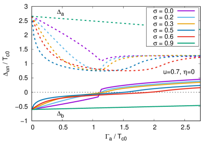
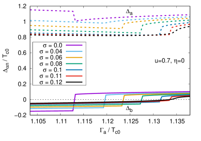
Figure 1: Matsubara gaps $\Delta_{\alpha n=1}$ dependence on the nonmagnetic impurity scattering rate $\Gamma_{a}$ for the $s_{\pm}$ state with $\eta=0$ and $T=0.03T_{c0}$. In the upper panel, we show a wide range of $\sigma$’s, while the data in lower panel demonstrate a jump in gaps at the point of the $s_{\pm}\to s_{++}$ transition for small values of $\sigma$. Note the smooth behavior of gaps for $\sigma>0.11$.

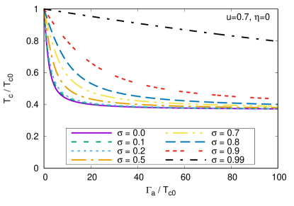
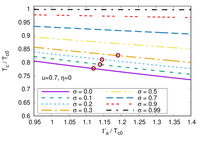
Figure 2: $T_{c}$ vs. scattering rate $\Gamma_{a}$ for the $s_{\pm}$ state with $\eta=0$. Results for a wide range of $\Gamma_{a}$’s is shown in the upper panel. In the lower panel, we show a narrow range of $\Gamma_{a}$’s where the $s_{\pm}\to s_{++}$ transition with jumps in gaps takes place. $T_{c}$ reveals smooth behavior at points of transition, which are marked by circles.

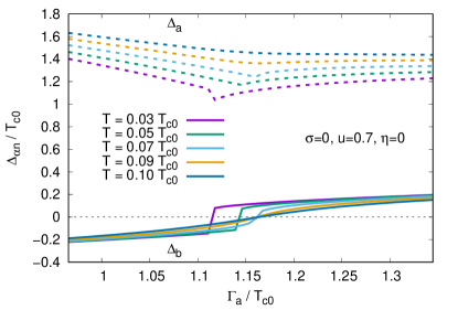
Figure 3: Temperature evolution of Matsubara gaps $\Delta_{\alpha n=1}$ for a range of $\Gamma_{a}$ with $\sigma=0$ and $\eta=0$. Note the steep behavior of smaller gaps at low temperatures and restoration of the smooth behavior for $T\gtrsim 0.09T_{c0}$.

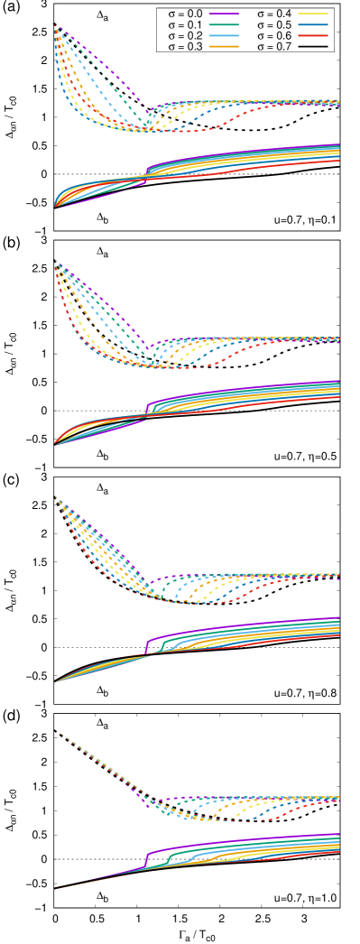
Figure 4: Matsubara gaps $\Delta_{\alpha n=1}$ vs. scattering rate $\Gamma_{a}$ in the $s_{\pm}$ state for various values of $\eta$, i.e., $v=0.1u$ (a), $v=u/2$ (b), $v=0.8u$ (c), and uniform impurity potential $v=u$ (d).

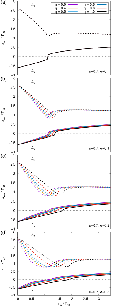
Figure 5: Matsubara gaps $\Delta_{\alpha n=1}$ vs. scattering rate $\Gamma_{a}$ in the $s_{\pm}$ state with varying $\eta$ for $\sigma=0$ (a), $\sigma=0.1$ (b), $\sigma=0.2$ (c), and $\sigma=0.3$ (d). In panel (a), all curves for different $\eta$ overlap.

Here we choose the relation between densities of states as $N_{b}/N_{a}=2$ and the following coupling constants: $(\lambda_{aa},\lambda_{ab},\lambda_{ba},\lambda_{bb})=(3,-0.2,-0.1,0.5)$. This gives the $s_{\pm}$ state with the superconducting critical temperature $T_{c0}$ of 40 K in the clean limit [61, 62, 50] and the positive averaged coupling constant, $\langle\lambda\rangle>0$, where $\langle\lambda\rangle\equiv(\lambda_{aa}+\lambda_{ab})N_{a}/N+(\lambda_{ba}+\lambda_{bb})N_{b}/N$ [50].

Since we are interested in behavior of gaps across the $s_{\pm}\to s_{++}$ transition, in Figure 1 we plot $\Delta_{\alpha n}$ for the first Matsubara frequency $n=1$ as functions of $\Gamma_{a}$ at $T=0.03T_{c0}$. Following the $b$-band behavior, we observe the transition for $\Gamma_{a}\gtrsim 1.1T_{c0}$. While for large values of $\eta$ the gaps changes smoothly across zero, for $\sigma<0.12$ we notice a jump in the smaller gap, $\Delta_{bn}$, when it crosses zero. It happens even in the Born limit, $\sigma=0$. At the same time, critical temperature is always a smooth function of $\Gamma_{a}$, see the $T_{c}$ plot in Figure 2. Critical temperature seems to ‘do not care’ about the jump occurring in the behavior of the smaller gap. To understand why this happens, we studied the temperature evolution of gaps. Results for $\sigma=0$ and $\eta=0$ are shown in Figure 3. Apparently, with increasing temperature, the steep behavior of $\Delta_{bn}$ changes to the smooth dependence on the scattering rate. This happens at $T\sim 0.1T_{c0}$ and, naturally, at higher temperatures, including $T_{c}$, the system shows smooth behavior. We have checked that the temperature dependence of gaps shown in Figure 3 stays the same for $\eta=0.5$ and $\eta=1$.

It is known that the strongest $T_{c}$ suppression takes place in the Born limit with $\eta=0$, while in the opposite limit of pure intraband scattering with $u=0$ ($\eta\to\infty$), pairbreaking is absent because $\tilde{\Gamma}_{ab}\to 0$ [32]. Similar situation is also characteristic for the unitary limit with $\sigma=1$, see equation (17).

To demonstrate, how the transition evolves with the increasing intraband part of the impurity potential, $v$, in Figures 4 and 5 we show results for different values of $\eta$ at $T=0.03T_{c0}$. Thus, in Figure 4, we go from almost pure interband to uniform scattering. Apparently, the critical $\Gamma_{a}$ at which the transition takes place increases with increasing $v$ for $\sigma>0$. In the Born limit, we observe the jump in the gaps for all $\eta$’s at exactly the same critical $\Gamma_{a}$, see Figure 5(a).

5 Conclusions

Here we studied the details of the $s_{\pm}\to s_{++}$ transition in the two-band model for the nonmagnetic impurity scattering in iron-based superconductors. We show that the gaps changes smoothly across the transition for all values of the cross-section parameter $\sigma$ and intra- to interband impurity potentials ratio $\eta$, except for the case of a weak scattering with small values of $\sigma$. In the latter case, the smaller gap changes steeply at the transition point. For the larger scattering rate $\Gamma_{a}$, the smaller gap evolves smoothly. The behavior changes around $\sigma=0.11$. With increasing temperature, the behavior of the gaps changes from the steep to the smooth around $T\sim 0.1T_{c0}$ for all values of $\sigma$ and $\eta$. That is the reason why the critical temperature is always a smooth function of the scattering rate $\Gamma_{a}$ and doesn’t care for steep changes in the behavior of the gaps.

References

References

- [1] Mazin I I 2010 Nature 464 183–186 ISSN 0028-0836 URL http://dx.doi.org/10.1038/nature08914
- [2] Sadovskii M V 2008 Phys. Usp. 51 1201–1227 URL https://ufn.ru/en/articles/2008/12/b/
- [3] Hirschfeld P J, Korshunov M M and Mazin I I 2011 Reports on Progress in Physics 74 124508 URL http://stacks.iop.org/0034-4885/74/i=12/a=124508
- [4] Reid J P, Juneau-Fecteau A, Gordon R T, de Cotret S R, Doiron-Leyraud N, Luo X G, Shakeripour H, Chang J, Tanatar M A, Kim H, Prozorov R, Saito T, Fukazawa H, Kohori Y, Kihou K, Lee C H, Iyo A, Eisaki H, Shen B, Wen H H and Taillefer L 2012 Superconductor Science and Technology 25 084013 URL http://stacks.iop.org/0953-2048/25/i=8/a=084013
- [5] Hosono H and Kuroki K 2015 Physica C: Superconductivity and its Applications 514 399 – 422 ISSN 0921-4534 superconducting Materials: Conventional, Unconventional and Undetermined URL http://www.sciencedirect.com/science/article/pii/S0921453415000477
- [6] Hirschfeld P J 2016 Comptes Rendus Physique 17 197 – 231 ISSN 1631-0705 URL http://www.sciencedirect.com/science/article/pii/S1631070515001693
- [7] Stewart G R 2011 Rev. Mod. Phys. 83(4) 1589–1652 URL http://link.aps.org/doi/10.1103/RevModPhys.83.1589
- [8] Muschler B, Prestel W, Hackl R, Devereaux T P, Analytis J G, Chu J H and Fisher I R 2009 Phys. Rev. B 80(18) 180510 URL http://link.aps.org/doi/10.1103/PhysRevB.80.180510
- [9] Canfield P C and Bud’ko S L 2010 Annual Review of Condensed Matter Physics 1 27–50 (Preprint https://doi.org/10.1146/annurev-conmatphys-070909-104041) URL https://doi.org/10.1146/annurev-conmatphys-070909-104041
- [10] Kemper A F, Korshunov M M, Devereaux T P, Fry J N, Cheng H P and Hirschfeld P J 2011 Phys. Rev. B 83 184516
- [11] Lumsden M D and Christianson A D 2010 Journal of Physics: Condensed Matter 22 203203 URL http://stacks.iop.org/0953-8984/22/i=20/a=203203
- [12] Fisher I R, Degiorgi L and Shen Z X 2011 Reports on Progress in Physics 74 124506 URL http://stacks.iop.org/0034-4885/74/i=12/a=124506
- [13] Dai P 2015 Rev. Mod. Phys. 87(3) 855–896 URL https://link.aps.org/doi/10.1103/RevModPhys.87.855
- [14] Inosov D S 2016 Comptes Rendus Physique 17 60 – 89 ISSN 1631-0705 URL http://www.sciencedirect.com/science/article/pii/S1631070515000523
- [15] Ding H, Richard P, Nakayama K, Sugawara K, Arakane T, Sekiba Y, Takayama A, Souma S, Sato T, Takahashi T, Wang Z, Dai X, Fang Z, Chen G F, Luo J L and Wang N L 2008 EPL (Europhysics Letters) 83 47001 URL http://stacks.iop.org/0295-5075/83/i=4/a=47001
- [16] Richard P, Sato T, Nakayama K, Takahashi T and Ding H 2011 Reports on Progress in Physics 74 124512 URL http://stacks.iop.org/0034-4885/74/i=12/a=124512
- [17] Kordyuk A A 2012 Low Temperature Physics 38 888–899 URL http://scitation.aip.org/content/aip/journal/ltp/38/9/10.1063/1.4752092
- [18] Zi-Rong Y, Yan Z, Bin-Ping X and Dong-Lai F 2013 Chinese Physics B 22 087407 URL http://stacks.iop.org/1674-1056/22/i=8/a=087407
- [19] Kordyuk A A 2015 Low Temperature Physics 41 319–341 URL http://scitation.aip.org/content/aip/journal/ltp/41/5/10.1063/1.4919371
- [20] Fujioka M, Denholme S J, Tanaka M, Takeya H, Yamaguchi T and Takano Y 2014 Applied Physics Letters 105 102602 URL http://scitation.aip.org/content/aip/journal/apl/105/10/10.1063/1.4895574
- [21] Qing-Yan W, Zhi L, Wen-Hao Z, Zuo-Cheng Z, Jin-Song Z, Wei L, Hao D, Yun-Bo O, Peng D, Kai C, Jing W, Can-Li S, Ke H, Jin-Feng J, Shuai-Hua J, Ya-Yu W, Li-Li W, Xi C, Xu-Cun M and Qi-Kun X 2012 Chinese Physics Letters 29 037402 URL http://stacks.iop.org/0256-307X/29/i=3/a=037402
- [22] Liu D, Zhang W, Mou D, He J, Ou Y B, Wang Q Y, Li Z, Wang L, Zhao L, He S, Peng Y, Liu X, Chen C, Yu L, Liu G, Dong X, Zhang J, Chen C, Xu Z, Hu J, Chen X, Ma X, Xue Q and Zhou X J 2012 Nat. Commun. 3 931 URL http://dx.doi.org/10.1038/ncomms1946
- [23] He S, He J, Zhang W, Zhao L, Liu D, Liu X, Mou D, Ou Y B, Wang Q Y, Li Z, Wang L, Peng Y, Liu Y, Chen C, Yu L, Liu G, Dong X, Zhang J, Chen C, Xu Z, Chen X, Ma X, Xue Q and Zhou X J 2013 Nat Mater 12 605–610 ISSN 1476-1122 URL http://dx.doi.org/10.1038/nmat3648
- [24] Tan S, Zhang Y, Xia M, Ye Z, Chen F, Xie X, Peng R, Xu D, Fan Q, Xu H, Jiang J, Zhang T, Lai X, Xiang T, Hu J, Xie B and Feng D 2013 Nat Mater 12 634–640 ISSN 1476-1122 URL http://dx.doi.org/10.1038/nmat3654
- [25] Ge J F, Liu Z L, Liu C, Gao C L, Qian D, Xue Q K, Liu Y and Jia J F 2015 Nat Mater 14 285–289 ISSN 1476-1122 URL http://dx.doi.org/10.1038/nmat4153
- [26] Korshunov M M 2014 Physics-Uspekhi 57 813–819 URL http://stacks.iop.org/1063-7869/57/i=8/a=813
- [27] Kontani H and Onari S 2010 Phys. Rev. Lett. 104(15) 157001 URL http://link.aps.org/doi/10.1103/PhysRevLett.104.157001
- [28] Bang Y, Choi H Y and Won H 2009 Phys. Rev. B 79(5) 054529 URL http://link.aps.org/doi/10.1103/PhysRevB.79.054529
- [29] Onari S and Kontani H 2012 Phys. Rev. B 85(13) 134507 URL http://link.aps.org/doi/10.1103/PhysRevB.85.134507
- [30] Onari S and Kontani H 2012 Phys. Rev. Lett. 109(13) 137001 URL https://link.aps.org/doi/10.1103/PhysRevLett.109.137001
- [31] Yamakawa Y and Kontani H 2017 Phys. Rev. B 96(4) 045130 URL https://link.aps.org/doi/10.1103/PhysRevB.96.045130
- [32] Korshunov M M, Togushova Y N and Dolgov O V 2016 Journal of Superconductivity and Novel Magnetism 29 1089–1095 ISSN 1557-1947 URL http://dx.doi.org/10.1007/s10948-016-3385-6
- [33] Anderson P 1959 Journal of Physics and Chemistry of Solids 11 26–30 ISSN 0022-3697 URL http://www.sciencedirect.com/science/article/pii/0022369759900368
- [34] Abrikosov A A and Gor’kov L P 1961 Sov. Phys. JETP 12 1243–1253
- [35] Karkin A E, Werner J, Behr G and Goshchitskii B N 2009 Phys. Rev. B 80(17) 174512 URL http://link.aps.org/doi/10.1103/PhysRevB.80.174512
- [36] Cheng P, Shen B, Hu J and Wen H H 2010 Phys. Rev. B 81(17) 174529 URL http://link.aps.org/doi/10.1103/PhysRevB.81.174529
- [37] Li Y, Tong J, Tao Q, Feng C, Cao G, Chen W, chun Zhang F and an Xu Z 2012 New Journal of Physics 12 083008 URL http://stacks.iop.org/1367-2630/12/i=8/a=083008
- [38] Nakajima Y, Taen T, Tsuchiya Y, Tamegai T, Kitamura H and Murakami T 2010 Phys. Rev. B 82(22) 220504 URL http://link.aps.org/doi/10.1103/PhysRevB.82.220504
- [39] Tropeano M, Cimberle M R, Ferdeghini C, Lamura G, Martinelli A, Palenzona A, Pallecchi I, Sala A, Sheikin I, Bernardini F, Monni M, Massidda S and Putti M 2010 Phys. Rev. B 81(18) 184504 URL http://link.aps.org/doi/10.1103/PhysRevB.81.184504
- [40] Kim H, Tanatar M A, Liu Y, Sims Z C, Zhang C, Dai P, Lograsso T A and Prozorov R 2014 Phys. Rev. B 89(17) 174519 URL http://link.aps.org/doi/10.1103/PhysRevB.89.174519
- [41] Prozorov R, Kończykowski M, Tanatar M A, Thaler A, Bud’ko S L, Canfield P C, Mishra V and Hirschfeld P J 2014 Phys. Rev. X 4(4) 041032 URL http://link.aps.org/doi/10.1103/PhysRevX.4.041032
- [42] Tarantini C, Putti M, Gurevich A, Shen Y, Singh R K, Rowell J M, Newman N, Larbalestier D C, Cheng P, Jia Y and Wen H H 2010 Phys. Rev. Lett. 104(8) 087002 URL http://link.aps.org/doi/10.1103/PhysRevLett.104.087002
- [43] Tan D, Zhang C, Xi C, Ling L, Zhang L, Tong W, Yu Y, Feng G, Yu H, Pi L, Yang Z, Tan S and Zhang Y 2011 Phys. Rev. B 84(1) 014502 URL http://link.aps.org/doi/10.1103/PhysRevB.84.014502
- [44] Grinenko V, Kikoin K, Drechsler S L, Fuchs G, Nenkov K, Wurmehl S, Hammerath F, Lang G, Grafe H J, Holzapfel B, van den Brink J, Büchner B and Schultz L 2011 Phys. Rev. B 84(13) 134516 URL http://link.aps.org/doi/10.1103/PhysRevB.84.134516
- [45] Li J, Guo Y F, Zhang S B, Yuan J, Tsujimoto Y, Wang X, Sathish C I, Sun Y, Yu S, Yi W, Yamaura K, Takayama-Muromachiu E, Shirako Y, Akaogi M and Kontani H 2012 Phys. Rev. B 85(21) 214509 URL http://link.aps.org/doi/10.1103/PhysRevB.85.214509
- [46] Golubov A A and Mazin I I 1997 Phys. Rev. B 55(22) 15146–15152 URL http://link.aps.org/doi/10.1103/PhysRevB.55.15146
- [47] Ummarino G 2007 Journal of Superconductivity and Novel Magnetism 20 639–642 ISSN 1557-1939 URL http://dx.doi.org/10.1007/s10948-007-0259-y
- [48] Senga Y and Kontani H 2008 Journal of the Physical Society of Japan 77 113710 URL http://dx.doi.org/10.1143/JPSJ.77.113710
- [49] Onari S and Kontani H 2009 Phys. Rev. Lett. 103(17) 177001 URL http://link.aps.org/doi/10.1103/PhysRevLett.103.177001
- [50] Efremov D V, Korshunov M M, Dolgov O V, Golubov A A and Hirschfeld P J 2011 Phys. Rev. B 84(18) 180512 URL http://link.aps.org/doi/10.1103/PhysRevB.84.180512
- [51] Efremov D V, Golubov A A and Dolgov O V 2013 New Journal of Physics 15 013002 URL http://stacks.iop.org/1367-2630/15/i=1/a=013002
- [52] Wang Y, Kreisel A, Hirschfeld P J and Mishra V 2013 Phys. Rev. B 87(9) 094504 URL https://link.aps.org/doi/10.1103/PhysRevB.87.094504
- [53] Korshunov M M, Efremov D V, Golubov A A and Dolgov O V 2014 Phys. Rev. B 90(13) 134517 URL http://link.aps.org/doi/10.1103/PhysRevB.90.134517
- [54] Yao Z J, Chen W Q, Li Y k, Cao G h, Jiang H M, Wang Q E, Xu Z a and Zhang F C 2012 Phys. Rev. B 86(18) 184515 URL http://link.aps.org/doi/10.1103/PhysRevB.86.184515
- [55] Chen H, Tai Y Y, Ting C S, Graf M J, Dai J and Zhu J X 2013 Phys. Rev. B 88(18) 184509 URL http://link.aps.org/doi/10.1103/PhysRevB.88.184509
- [56] Castellani C, Natoli C R and Ranninger J 1978 Phys. Rev. B 18(9) 4945–4966 URL http://link.aps.org/doi/10.1103/PhysRevB.18.4945
- [57] Oleś A M 1983 Phys. Rev. B 28(1) 327–339 URL http://link.aps.org/doi/10.1103/PhysRevB.28.327
- [58] Berk N F and Schrieffer J R 1966 Phys. Rev. Lett. 17(8) 433–435 URL http://link.aps.org/doi/10.1103/PhysRevLett.17.433
- [59] Allen P B and Mitrovic B 1982 Theory of superconducting Solid State Physics: Advances in Research and Applications vol 37 ed Erenreich H, Zeitz F and Turnbull D (New York: Academic) pp 1–92 ISBN 0126077371
- [60] Parker D, Dolgov O V, Korshunov M M, Golubov A A and Mazin I I 2008 Phys. Rev. B 78(13) 134524 URL https://link.aps.org/doi/10.1103/PhysRevB.78.134524
- [61] Popovich P, Boris A V, Dolgov O V, Golubov A A, Sun D L, Lin C T, Kremer R K and Keimer B 2010 Phys. Rev. Lett. 105(2) 027003 URL http://link.aps.org/doi/10.1103/PhysRevLett.105.027003
- [62] Charnukha A, Dolgov O V, Golubov A A, Matiks Y, Sun D L, Lin C T, Keimer B and Boris A V 2011 Phys. Rev. B 84(17) 174511 URL http://link.aps.org/doi/10.1103/PhysRevB.84.174511