Gene flow across geographical barriers - scaling limits of random walks with obstacles

Abstract

We study a class of random walks which behave like simple random walks outside of a bounded region around the origin and which are subject to a partial reflection near the origin. We obtain a non trivial scaling limit which behaves like reflected Brownian motion until its local time at zero reaches an exponential variable. It then follows reflected Brownian motion on the other side of the origin until its local time at zero reaches another exponential level, etc. These random walks are used in population genetics to trace the position of ancestors in the past near geographical barriers.

Keywords: generalised Brownian motions;random walks with obstacles;partial reflection;barriers to gene flow.
2010 MSC: 60G99, 60F99, 60J65, 60J70

Introduction

Barriers to gene flow are physical obstacles to migration. Examples include mountain ranges, highways, political borders and the Great Wall of China [28]. All these geographical features leave traces in the genetic composition of populations living on both sides of the barrier. Geneticists try to use these traces to detect barriers to gene flow and to quantify their effect on migration.

A naive approach to this problem would be to compute a measure of genetic differentiation (e.g. Wright’s F_st [29] which measures the level of inbreeding in the population resulting from its structure [24]) between the two populations on each side of the candidate barrier, and to say that the latter acts as a barrier to gene flow if two individuals living on the same side are more related to each other on average than two indivudals living on different sides of the barrier.

This method assumes that the two subpopulations on each side of the obstacle are well mixed. This may not always be a reasonable assumption and in some cases it is preferable to take into account the finer scale geographic structure of the sampled population.

Mathematical models for spatially extended populations with barriers to gene flow already exist in the literature [13, 27], but most assume a discrete space and finding analytical formulae in this framework is challenging at best. Such formulae are particularly useful for inference purposes, where computational power is limiting. This paper is a step towards a rigorous mathematical framework to model genetic isolation by distance with barriers to gene flow in a continuous space.

Stepping stone model with a barrier at the origin

Nagylaki and his co-authors proposed the following model for the evolution of a spatially structured population with a barrier to gene flow [13, 15, 17]. Consider a population living in a discrete linear space, with colonies (or demes) at locations $\{\ldots,-2,-1,1,2,\ldots\}$. Each deme contains $N$ individuals, and at each generation, those individuals are replaced by the offspring of the previous generation. An individual in deme $i\notin\{-1,1\}$ has its parent in the previous generation in deme $i-1$ or $i+1$ with probability $m/2$ for some $m\in(0,1)$, otherwise its parent is drawn from deme $i$. Individuals in deme $1$ have their parent in deme $2$ with probability $m/2$ and in deme $-1$ with probability $cm/2$, with $c\in(0,1)$, and likewise individuals in deme $-1$ have their parent in deme $1$ with probability $cm/2$. Migration probabilities are depicted in Figure 1. Properties of this model and applications to various settings were studied in a sequence of papers [13, 14, 19, 16, 20].

Figure 1: Stepping stone model with a barrier to gene flow

In this model, two individuals sampled at a given distance from each other will be more related if they are sampled on the same side of the origin than if they are not. This can be seen by assuming that each new individual mutates to a type never seen before with some probability $\mu\in(0,1)$. Relatedness between individuals can then be measured by the probability that two sampled individuals are of the same type. This probability is called the probability of identity by descent, and it is given by the probability generating function of the age of the most recent common ancestor of these individuals. Properties of this function were studied in this setting in [2].

Also of interest is the evolution of the frequency of a given type (or allele) in the population, denoted by $(p^{N}(t,x),x\in\mathbb{Z}\setminus\{0\},t\geq 0)$. Ignoring mutations and setting

$$\bar{p}(t,x)=\mathbb{E}\left[p^{N}(t,x)\right],$$

$\bar{p}$ solves a simple difference equation. Setting

$$\bar{p}_{n}(t,x)=\bar{p}(nt,\sqrt{n}x)$$

for $n\geq 1$ and assuming that $\sqrt{n}c\to\gamma\in(0,\infty)$, Nagylaki [13] showed that $\bar{p}_{n}$ converges to the solution of the following equation

$$\begin{cases}\partial_{t}p(t,x)=\frac{\sigma^{2}}{2}\partial_{xx}p(t,x)\qquad\text{ for }x\in\mathbb{R}\setminus\{0\},\\ \partial_{x}p(t,0^{-})=\partial_{x}p(t,0^{+})=\gamma(p(t,0^{+})-p(t,0^{-}))\end{cases}$$ (1)

where $\sigma^{2}=m$, see Figure 2. In [14] (see also [2]), Nagylaki showed a similar approximation for the probability of identity by descent.

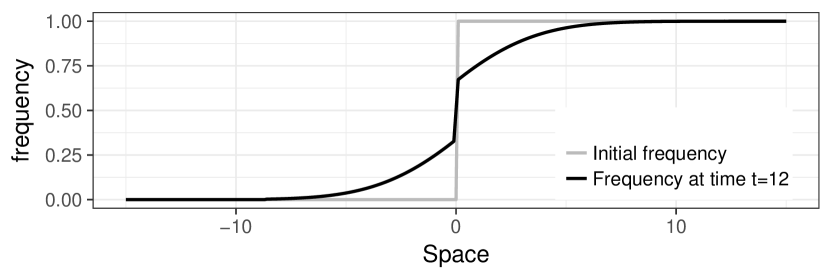
Figure 2: Evolution of allele frequency

Frequency of a type initially present at the right of the origin after a few generations.

Duality

An alternative way to study this model from the forwards in time evolution of types is to look back in time for the position of one’s ancestor some number of generations in the past. If $\xi^{x}_{t}$ denotes the position of the ancestor $t$ generations ago of an individual sampled at $x\in\mathbb{Z}\setminus\{0\}$, then $(\xi^{x}_{t},t\geq 0)$ is a random walk with transition probabilities given by the migration rates in Figure 1. In the absence of mutations, the proportion of individuals carrying a given allele at location $x$ is the proportion of those individuals whose ancestor $t$ generations ago carried the same allele. As a result, for $x\in\mathbb{Z}\setminus\{0\}$ and $t\geq 0$,

$$\bar{p}(t,x)=\mathbb{E}\left[p^{N}(0,\xi^{x}_{t})\right].$$

Likewise, the probability of identity by descent can be expressed with the help of the coalescence time of two random walks $\xi^{x},\xi^{y}$, i.e. the first time that the two ancestors have the same parent.

Scaling limits of random walks with obstacles

In this paper, we present a result on the scaling limits of a class of random walks with obstacles which includes $(\xi^{x}_{t},t\geq 0)$. For $n\geq 1$, if we set

$$X_{n}(t)=\frac{1}{\sqrt{n}}\xi_{nt}^{\lfloor\sqrt{n}x\rfloor},$$

and if $c$ is of order $n^{-1/2}$, we show that $X_{n}$ converges in distribution to a continuous stochastic process. This process resembles Brownian motion everywhere except near the origin where it has a singular behaviour. More precisely, this process behaves like reflected Brownian motion until its local time at the origin reaches an exponential random variable, after which it becomes reflected Brownian motion on the other side of the origin, until its local time reaches another exponential variable, and so on. We call this process partially reflected Brownian motion. It generalises elastic Brownian motion considered for example in [5].

The same process was obtained as a limit of one dimensional diffusions in [12]. For $\varepsilon>0$, they consider $(X_{\varepsilon}(t),t\geq 0)$, solution to

$$dX_{\varepsilon}(t)=\frac{L_{\varepsilon}}{\varepsilon}a\left(\frac{1}{\varepsilon}X_{\varepsilon}(t)\right)dt+dB_{t},$$

where $B$ is standard Brownian motion, $L_{\varepsilon}\to\infty$ as $\varepsilon\downarrow 0$ and $\operatorname{sign}(x)a(x)\geq 0$, $supp(a)\subset[-1,1]$, and they give conditions on $L_{\varepsilon}$ under which $X_{\varepsilon}$ converges to partially reflected Brownian motion (which they call Brownian motion with a hard membrane).

This process also appears in [10] under the name snapping out Brownian motion and is obtained as a limit of one dimensional diffusions with a small diffusivity in a thin layer around the origin. Lejay also gives another construction by piecing together a sequence of elastic Brownian motions, choosing their sign at random each time the process is killed and reborn.

In addition, we give a different construction of partially reflected Brownian motion inspired by the speed and scale construction of one dimensional diffusions. Starting with standard Brownian motion, we glue together its excursions above level $x>0$ and below level $-x$ and we show that the result is the same process as the one described above.

Moreover, we provide a martingale problem characterisation of partially reflected Brownian motion, where equation (1) can be seen as the action of the semigroup of partially reflected Brownian motion on the initial allele frequency. In particular, the domain of the infinitesimal generator associated to partially reflected Brownian motion is precisely the space of twice continuously differentiable functions on $\mathbb{R}\setminus\{0\}$ satisfying

$$\dfrac{dp}{dx}(0^{+})=\dfrac{dp}{dx}(0^{-})=\gamma(p(0^{+})-p(0^{-}))$$

for some $\gamma>0$.

We also provide an explicit formula for the transition density of partially reflected Brownian motion in Corollary 1.6 below. It turns out that this transition density has already been in use in the field of diffusion in porous media [18, 6], but without mention of the underlying stochastic process.

More recently, this process has been used in [22] to detect barriers to gene flow in genetic samples and to measure their strength from the resulting distortion in isolation by distance patterns.

This paper is laid out as follows. In Section 1, we present our main results: partially reflected Brownian motion is defined as the solution to a martingale problem and two constructions of this process are given, we also state the convergence of a class of random walks to partially reflected Brownian motion. In Section 2, we prove that the martingale problem which charaterizes partially reflected Brownian motion is well posed and we show that the two constructions in Section 1 provide solutions to this martingale problem. Finally in Section 3, we prove the convergence in distribution of a sequence of random walks to partially reflected Brownian motion.

1 Main results

1.1 Definition and constructions of partially reflected Brownian motion

We first give a definition of partially reflected Brownian motion as a solution to a martingale problem on a space consisting of the disjoint union of the positive and negative half lines. We will show that this martingale problem is well posed. We then give two constructions of this process.

Definition

Let $\ddot{\mathbb{R}}$ be the disjoint union of the positive and negative half lines,

$$\ddot{\mathbb{R}}=(-\infty,0^{-}]\cup[0^{+},+\infty).$$

It is endowed with the metric $d$ defined by

$$\forall x,y\in\ddot{\mathbb{R}},\quad d(x,y)=\left|x-y\right|+\mathds{1}_{\left\{xy\leq 0\right\}}.$$

Let $\hat{C}(\ddot{\mathbb{R}})$ be the set of continuous real-valued functions on $\ddot{\mathbb{R}}$ which vanish at infinity. For $\gamma\in[0,+\infty]$, let $\mathcal{D}^{\gamma}$ be the subspace of functions $f\in\hat{C}(\ddot{\mathbb{R}})$ which are twice continuously differentiable on each half line and satisfy

$$\dfrac{df}{dx}(0^{-})=\dfrac{df}{dx}(0^{+})=\gamma(f(0^{+})-f(0^{-})).$$ (2)

(For $\gamma=+\infty$, (2) becomes $f^{\prime}(0^{-})=f^{\prime}(0^{+})$ and $f(0^{-})=f(0^{+})$.) Fix $\sigma>0$ and let us define a linear operator $L^{\gamma}$ on $\mathcal{D}^{\gamma}$ by

$$L^{\gamma}f=\frac{\sigma^{2}}{2}\dfrac{d^{2}f}{dx^{2}},\quad\forall f\in\mathcal{D}^{\gamma}.$$ (3)

Let $D(\mathbb{R}_{+},\ddot{\mathbb{R}})$ denote the space of càdlàg functions from $\mathbb{R}_{+}$ to $\ddot{\mathbb{R}}$.

Definition 1.1 (partially reflected Brownian motion).

Let $\left(X_{t}\right)_{t\geq 0}$ be a càdlàg, $\ddot{\mathbb{R}}$-valued Markov process on a probability space $\left(\Omega,\mathcal{A},\mathbb{P}\right)$, and call $\mathbb{P}^{X}$ its law on $D(\mathbb{R}_{+},\ddot{\mathbb{R}})$. The process $\left(X_{t}\right)_{t\geq 0}$ (resp. its law $\mathbb{P}^{X}$) is said to be (the law of) partially reflected Brownian motion if it is a solution to the martingale problem associated with $L^{\gamma}$ for some $\gamma\in[0,+\infty]$, i.e. if for any $f\in\mathcal{D}^{\gamma}$, the process

$$f(X_{t})-\int_{0}^{t}L^{\gamma}f(X_{s})ds$$ (4)

is a martingale with respect to the filtration generated by $\left(X_{t}\right)_{t\geq 0}$. We call $\gamma$ the permeability of the barrier.

Naturally, we say that $\left(X_{t}\right)_{t\geq 0}$ is partially reflected Brownian motion with initial distribution $\mu$ if it is a solution to the martingale problem associated with $(L^{\gamma},\mu)$, i.e. if (4) is a martingale for all $f\in\mathcal{D}^{\gamma}$ and if $\mathbb{P}^{X}\left(X_{0}\in\cdot\right)=\mu(\cdot)$.

The operator $L^{\gamma}$ is thus the generator of partially reflected Brownian motion. This definition does not seem to provide much information about possible solutions to this martingale problem. It does not even tell us if such solutions exist or if they are unique (in distribution). This is the subject of the next proposition. Below, we also give two ways to construct solutions to this martingale problem.

It should be noted that for $\gamma=0$ (impermeable barrier), the operator $L^{\gamma}$ is the generator of reflected Brownian motion (see for example Exercice VII.1.23 in [23] in the case $\alpha=1$), while for $\gamma=+\infty$ (completely permeable barrier), $L^{\gamma}$ is the generator of Brownian motion.

Proposition 1.2.

For any $\gamma\in[0,+\infty]$, the martingale problem associated with $L^{\gamma}$ has at most one $D(\mathbb{R}_{+},\ddot{\mathbb{R}})$ valued solution.

Proof.

The operator $L^{\gamma}$ satisfies the positive maximum principle on $\mathcal{D}^{\gamma}$, i.e. whenever $f\in\mathcal{D}^{\gamma}$ and $\sup_{x\in\ddot{\mathbb{R}}}f(x)=f(x_{0})\geq 0$, we have $L^{\gamma}f(x_{0})\leq 0$. By Lemma 4.2.1 of [4], $L^{\gamma}$ is thus dissipative on $\mathcal{D}^{\gamma}$ (recall that we require the functions in $\mathcal{D}^{\gamma}$ to vanish at infinity).

Let us now show that for any positive $\lambda$, the range of $\lambda-L^{\gamma}$ contains the space $\hat{C}(\ddot{\mathbb{R}})$ of continuous functions vanishing at infinity. We do it in the case $\sigma^{2}=2$, but the general case is similar. Let $f\in\hat{C}(\ddot{\mathbb{R}})$ be such a function and define

$$g(x)=\left\{\begin{aligned} &e^{-\sqrt{\lambda}x}\int_{0}^{x}\dfrac{e^{\sqrt{\lambda}y}}{2\sqrt{\lambda}}f(y)dy+e^{\sqrt{\lambda}x}\int_{x}^{+\infty}\dfrac{e^{-\sqrt{\lambda}y}}{2\sqrt{\lambda}}f(y)dy+Ae^{-\sqrt{\lambda}x}&\text{ if }x\geq 0^{+},\\ &e^{-\sqrt{\lambda}x}\int_{-\infty}^{x}\dfrac{e^{\sqrt{\lambda}y}}{2\sqrt{\lambda}}f(y)dy+e^{\sqrt{\lambda}x}\int_{x}^{0}\dfrac{e^{-\sqrt{\lambda}y}}{2\sqrt{\lambda}}f(y)dy+Be^{\sqrt{\lambda}x}&\text{ if }x\leq 0^{-},\end{aligned}\right.$$

for some $A,B\in\mathbb{R}$. Then $g$ is twice continuously differentiable on $\ddot{\mathbb{R}}$, vanishes at infinity and satisfies

$$\dfrac{d^{2}g}{dx^{2}}(x)=\lambda g(x)-f(x)$$

for all $x\in\ddot{\mathbb{R}}$. The constants $A$ and $B$ can then be chosen so that $g$ also satisfies (2). As a result we have found a function $g$ in $\mathcal{D}^{\gamma}$ such that $\lambda g-L^{\gamma}g=f$ for any $f\in\hat{C}(\ddot{\mathbb{R}})$.

In particular, since $\mathcal{D}^{\gamma}$ is a subset of $\hat{C}(\ddot{\mathbb{R}})$, it is in the range of $\lambda-L^{\gamma}$ for any $\lambda>0$. Furthermore $\hat{C}(\ddot{\mathbb{R}})$ is separating in the sense of Section 3.4 in [4]. Proposition 1.2 then follows from Corollary 4.4.4 in [4]. ∎

"Speed and scale" construction of partially reflected Brownian motion

We now present a way to construct partially reflected Brownian motion from Brownian motion, via an analogy with the speed and scale construction of one dimensional diffusions. This will give us a better sense of what "typical" trajectories of this process look like. Indeed, we show that the excursions of partially reflected Brownian motion outside the origin are given by the sequence of excursions of a Brownian motion outside a macroscopic region of length $\frac{1}{\gamma}$, as illustrated in Figure 3.

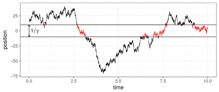
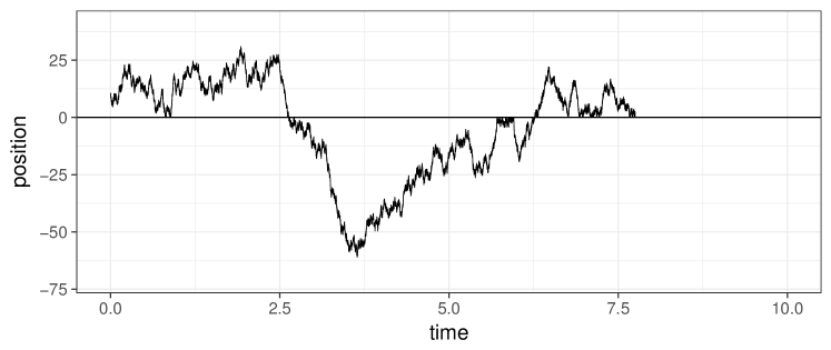
Figure 3: Speed and scale construction of partially reflected Brownian motion

Construction of partially reflected Brownian motion as a time-changed Brownian motion, with $\sigma^{2}=400$, $x=20$ and $\gamma=0.05$.

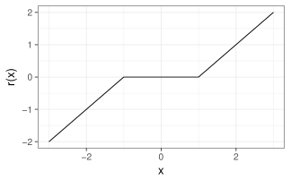
Figure 4: Graph of the function $r:\mathbb{R}\to\ddot{\mathbb{R}}$ for $\gamma=0.5$.

Fix $\gamma\in(0,+\infty)$ and suppose for simplicity that $\sigma^{2}=1$. Define $r:\mathbb{R}\to\ddot{\mathbb{R}}$ by

$$r(x)=\begin{cases}x-\frac{1}{2\gamma}&\text{ if }x>\frac{1}{2\gamma},\\ x+\frac{1}{2\gamma}&\text{ if }x<-\frac{1}{2\gamma},\\ 0^{+}&\text{ if }0\leq x\leq\frac{1}{2\gamma},\\ 0^{-}&\text{ if }-\frac{1}{2\gamma}\leq x<0,\end{cases}$$

(see Figure 4). Further define $r^{-1}:\ddot{\mathbb{R}}\to\mathbb{R}$ by

$$r^{-1}(x)=x+\operatorname{sign}(x)\frac{1}{2\gamma}.$$

(Note that $r^{-1}$ is only the right inverse of $r$, i.e. $r\circ r^{-1}=Id_{\ddot{\mathbb{R}}}$ but $r^{-1}\circ r\neq Id_{\mathbb{R}}$.) Now fix $x\in\ddot{\mathbb{R}}$ and let $\left(B_{t}\right)_{t\geq 0}$ be standard Brownian motion started from $r^{-1}(x)$. Also set, for $t\geq 0$,

$$\tau(t)=\inf\left\{\tau>0:\int_{0}^{\tau}\mathds{1}_{\left\{\left|B_{s}\right|>\frac{1}{2\gamma}\right\}}ds>t\right\}.$$ (5)

Finally, let $X_{t}=r(B_{\tau(t)})$.

Proposition 1.3.

The process $\left(X_{t}\right)_{t\geq 0}$ is partially reflected Brownian motion started from $x$, i.e. it is a solution to the martingale problem associated with $\left(L^{\gamma},\delta_{x}\right)$.

We prove this result in Subsection 2.1. The construction is illustrated in Figure 3. In words, we map the two intervals $(-\infty,-\frac{1}{2\gamma}]$ and $[\frac{1}{2\gamma},+\infty)$ onto $(-\infty,0^{-}]$ and $[0^{+},+\infty)$, and we change time in order to drop the time intervals where $\left|B_{s}\right|\leq\frac{1}{2\gamma}$.

Remark.

From this construction, we recover the property stated by Nagylaki [13, Equation 56] that, for $0<x<y$,

$$\mathbb{P}_{x}\left(X_{t}\text{ reaches $0^{-}$ before $y$}\right)=\frac{y-x}{y+\frac{1}{\gamma}}.$$

More generally, Proposition 1.3 shows that $r^{-1}$ is the scale function of partially reflected Brownian motion.

Corollary 1.4.

For any $\gamma\in[0,+\infty]$, the martingale problem associated to $L^{\gamma}$ is well posed, i.e. it has a unique solution.

Let $\ddot{\pi}:\ddot{\mathbb{R}}\to\mathbb{R}$ be the natural projection of $\ddot{\mathbb{R}}$ onto $\mathbb{R}$ (i.e. mapping both $0^{+}$ and $0^{-}$ onto $0$). We sometimes also call the projection $\left(\ddot{\pi}(X_{t})\right)_{t\geq 0}$ partially reflected Brownian motion, even though the latter isn’t a Markov process. (For example, as we shall see below, the sequence of random walks considered in Subsection 1.2 converges to the projection of partially reflected Brownian motion.)

Construction involving the local time at the origin

From the previous construction, one is led to think that $\left(\left|X_{t}\right|\right)_{t\geq 0}$ has the law of reflected Brownian motion. It is then natural to ask if partially reflected Brownian motion can be constructed by randomly "flipping" the excursions of reflected Brownian motion. The next proposition provides such a construction. It turns out that the crossing times of the origin are the times at which the local time at the origin of the process reaches the arrival times of an independent Poisson process with parameter $\gamma$, as in Figure 5.

Fix $x\in\ddot{\mathbb{R}}$ and let $\left(W_{t}\right)_{t\geq 0}$ be reflected Brownian motion on $\mathbb{R}_{+}$ started from $\left|x\right|$. Let $\left(N(t),t\geq 0\right)$ be a Poisson process with rate $\gamma\in(0,\infty)$, independent of $\left(W_{t}\right)_{t\geq 0}$. Let $L^{0}_{t}(W)$ denote the local time accumulated at the origin up to time $t$ by $W$, that is,

$$L^{0}_{t}(W)=\lim_{\varepsilon\downarrow 0}\frac{1}{2\varepsilon}\int_{0}^{t}\mathds{1}_{\left\{\left|W_{s}\right|\leq\varepsilon\right\}}ds$$

(see [23, Chapter VI]). Set

$$X_{t}=\operatorname{sign}(x)(-1)^{N(L^{0}_{t}(W))}W_{t},$$

where $\pm 1\times 0=0^{\pm}$ (see Figure 5).

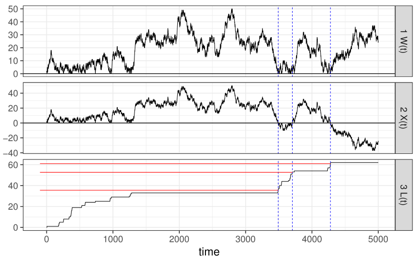
Figure 5: Construction of partially reflected Brownian motion involving the local time at the origin

Top graph shows a realisation of reflected Brownian motion $W_{t}$. Bottom graph shows its local time accumulated at the origin $L(t)$. The heights of horizontal red lines are drawn according to a Poisson process on the y axis. The graph in the middle is obtained by "flipping" $W_{t}$ at the times when $L(t)$ reaches the red lines. The corresponding process is distributed as the projection of partially reflected Brownian motion.

Proposition 1.5.

The process $\left(X_{t}\right)_{t\geq 0}$ is partially reflected Brownian motion started from $x$.

We prove this result in Subsection 2.2 using the previous construction and a Ray-Knight theorem [25, Theorem 6.4.7], which states that the local time accumulated by Brownian motion at $\frac{1}{2\gamma}$ before reaching $-\frac{1}{2\gamma}$ is an exponential random variable with parameter $\gamma$.

Proposition 1.5 yields an explicit formula for the transition density of partially reflected Brownian motion. For $t>0$ and $x\in\mathbb{R}$, set

$$G_{t}(x)=\frac{1}{\sqrt{2\pi t}}\exp\left(-\frac{x^{2}}{2t}\right).$$

Corollary 1.6.

If $\left(X_{t}\right)_{t\geq 0}$ is partially reflected Brownian motion with permeability $\gamma\in(0,\infty)$ started from $x\in\ddot{\mathbb{R}}$, then $\mathbb{P}_{x}\left(X_{t}\in dy\right)=g_{t}(x,y)dy$ with

$$g_{t}(x,y)=\begin{cases}G_{t}(x-y)+G_{t}(x+y)-2\gamma\int_{0}^{+\infty}e^{-2\gamma l}G_{t}(\left|x\right|+\left|y\right|+l)dl&\text{ if }xy\geq 0^{+},\\ 2\gamma\int_{0}^{+\infty}e^{-2\gamma l}G_{t}(\left|x\right|+\left|y\right|+l)dl&\text{ if }xy\leq 0^{-}.\end{cases}$$

We derive this formula in Subsection 2.4.

1.2 Scaling limits of a class of random walks

Let us now state the main convergence result, namely that partially reflected Brownian motion is the scaling limit of a class of random walks with an obstacle. We consider a more general case than [13], where the barrier to gene flow has width $K\in\mathbb{N}\setminus\{0\}$ ($K$ being the number of edges with reduced migration rate). The cases $K=1$ (the one considered in [13]) and $K=2$ are illustrated in Figure 6. We define the process describing the motion of an ancestral lineage as follows.

a)

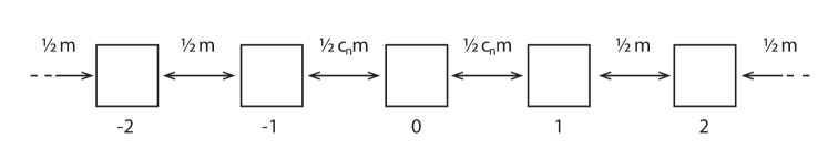
b) Transition rates of the random walk $(\xi_{n}(t),t\geq 0)$ in a) case $K=1$ and $b)$ case $K=2$.

Figure 6: Jump rates of random walks with an obstacle

Definition 1.7 (Random walk with an obstacle).

Let $\left(c_{n}\right)_{n\geq 1}$ be a sequence of positive real numbers, and fix $m>0$. Suppose that $\left(x_{n}^{0}\right)_{n\geq 1}$ is a sequence of elements of $\mathbb{N}^{*}$.

If $K$ is even,

let $E=\mathbb{Z}$ and define, for $i\neq j\in E$,

$$q_{n}(i,j)=\begin{cases}\frac{m}{2}&\text{ if }\left|i-j\right|=1\text{ and }\left|i\right|\vee\left|j\right|>\frac{K}{2},\\ c_{n}\frac{m}{2}&\text{ if }\left|i-j\right|=1\text{ and }\left|i\right|\vee\left|j\right|\leq\frac{K}{2},\\ 0&\text{ otherwise.}\end{cases}$$ (6)

If $K$ is odd,

let $E=\mathbb{Z}\setminus\{0\}$ and set, for $i\neq j\in E$,

$$q_{n}(i,j)=\begin{cases}\frac{m}{2}&\text{ if }\left|i-j\right|=1\text{ and }\left|i\right|\vee\left|j\right|>\frac{K+1}{2},\\ c_{n}\frac{m}{2}&\text{ if }\left|i-j\right|=1\text{ and }\left|i\right|\vee\left|j\right|\leq\frac{K+1}{2},\\ &\text{ or if }\{i,j\}=\{+1,-1\},\\ 0&\text{ otherwise.}\end{cases}$$ (7)

Then let $\left(\xi_{n}(t),t\geq 0\right)$ be a continuous time random walk on $E$ started from $x_{n}^{0}$ with jump rates $q_{n}(\cdot,\cdot)$. That is, whenever $\xi_{n}(t)=i$, the future of the random walk is determined as follows. Attach to each $j\neq i$ in $E$ such that $q_{n}(i,j)>0$ an independent exponential random variable $E_{j}$ with parameter $q_{n}(i,j)$. Then at time $J_{1}=t+\inf\{E_{j}\}$, the random walk jumps to state $k=\operatorname*{arg\,min}_{j}\{E_{j}\}$. This procedure is then repeated between each jump time of the random walk.

For $n\geq 1$, set $X_{n}(t)=\frac{1}{\sqrt{n}}\xi_{n}(nt)$. We now state conditions under which the rescaled random walk $X_{n}=(X_{n}(t),t\geq 0)$ converges to partially reflected Brownian motion. We equip the space of càdlàg functions from $\mathbb{R}_{+}$ to $\mathbb{R}$ (denoted by $\mathrm{D}\left(\mathbb{R}_{+},\mathbb{R}\right)$) with the topology of Skorokhod convergence on compact time intervals. If $d_{sko}^{T}(\cdot,\cdot)$ is a metric for the Skorokhod convergence on $\mathrm{D}\left({[0,T]},\mathbb{R}\right)$ for $T>0$, then

$$d_{sko}(f,g)=\int_{0}^{+\infty}e^{-t}(d_{sko}^{t}(f,g)\wedge 1)dt$$ (8)

is a metric for Skorokhod convergence on compact time intervals.

Theorem 1.

Suppose $\frac{1}{\sqrt{n}}x_{n}^{0}\underset{n\to\infty}{\longrightarrow}x^{0}$ with $x^{0}\neq 0$ and $\lim_{n\to\infty}\frac{\sqrt{n}}{K}c_{n}=\gamma\in[0,+\infty]$. Then as $n\to\infty$, the sequence of real-valued processes $\left(X_{n}(t),t\geq 0\right)$ converges in distribution in $(\mathrm{D}\left(\mathbb{R}_{+},\mathbb{R}\right),d_{sko})$ to a continuous real-valued process $(X(t),t\geq 0)$ which is (a projection on $\mathbb{R}$ of) a solution to the martingale problem associated with $\left(L^{\gamma},\delta_{x^{0}}\right)$, with $\sigma^{2}=m$.

In other words, if $\sqrt{n}c_{n}\to+\infty$, $X_{n}$ converges to Brownian motion, if $\sqrt{n}c_{n}\to 0$, $X_{n}$ converges to reflected Brownian motion, while if $\frac{\sqrt{n}}{K}c_{n}\to\gamma\in(0,\infty)$, $X_{n}$ converges to (the projection of) partially reflected Brownian motion (recall that the latter takes values in $\ddot{\mathbb{R}}$, its projection is obtained by identifying $0^{+}$ and $0^{-}$ with $0$).

Remark.

In the case $x^{0}=0$, the convergence still holds provided the probability of first exiting the set $[-K/2,K/2]$ on the right converges as $n\to\infty$. The initial distribution is then a convex combination of $\delta_{0^{+}}$ and $\delta_{0^{-}}$, given by the limits of the exit probabilities.

Theorem 1 is proved in Section 3 in the case $K=2$. The generalisation to other values of $K$ is straighforward, and the case $K=1$ introduces some simplifications, which makes the case $K=2$ more representative of the general case.

Note that in Nagylaki’s model presented in Figure 1, ancestral lineages are distributed as the random walk of Definition 1.7 with $K=1$.

2 Constructions of partially reflected Brownian motion

2.1 Speed and scale construction

Here we prove that the process $X_{t}=r(B_{\tau(t)})$ defined in Subsection 1.1 is a solution to the martingale problem associated with $L^{\gamma}$. This proof will require the following lemma, proved in Subsection 2.3.

Lemma 2.1.

Set $W_{t}=\left|X_{t}\right|$. Then $\left(W_{t}\right)_{t\geq 0}$ is distributed as reflected Brownian motion.

Proof of Proposition 1.3.

Recall that $B$ is standard Brownian motion started at $r^{-1}(x)$, hence $X_{0}=x$ almost surely. Let $\left(\mathcal{F}^{B}_{t}\right)_{t\geq 0}$ denote the natural filtration of $\left(B_{t}\right)_{t\geq 0}$, and let $\mathcal{F}_{t}=\mathcal{F}^{B}_{\tau(t)}$. Then $\left(\mathcal{F}_{t}\right)_{t\geq 0}$ is a filtration, $\left(X_{t}\right)_{t\geq 0}$ is $\left(\mathcal{F}_{t}\right)_{t\geq 0}$ adapted and, for $s,t\geq 0$ and $f:\ddot{\mathbb{R}}\to\mathbb{R}$ bounded and continuous,

$$\mathbb{E}\left[\left.f(X_{t+s})\>\right|\>\mathcal{F}_{t}\right]=\mathbb{E}_{r^{-1}(X_{t})}\left[f(r(B_{\tau(s)}))\right].$$

Hence $(X_{t},t\geq 0)$ is a Markov process with respect to $(\mathcal{F}_{t},t\geq 0)$. Now let $\left(\mathcal{F}^{X}_{t}\right)_{t\geq 0}$ be the filtration generated by $\left(X_{t}\right)_{t\geq 0}$. Since $\mathcal{F}^{X}_{t}\subset\mathcal{F}_{t}$, $\left(X_{t}\right)_{t\geq 0}$ is a Markov process with respect to $(\mathcal{F}^{X}_{t},t\geq 0)$.

Suppose now that for any $x\in\ddot{\mathbb{R}}$ and $f\in\mathcal{D}^{\gamma}$,

$$\lim_{t\downarrow 0}\dfrac{1}{t}\mathbb{E}_{x}\left[f(X_{t})-f(X_{0})\right]=\dfrac{1}{2}\dfrac{d^{2}f}{dx^{2}}(x).$$ (9)

(Recall that we assumed $\sigma^{2}=1$ for simplicity.) Then, by Proposition 4.1.7 in [4], (4) is an $\mathcal{F}^{X}$-martingale for all $f\in\mathcal{D}^{\gamma}$ ($X$ is progressive since it is right-continuous). It follows that $\left(X_{t}\right)_{t\geq 0}$ is a solution to the martingale problem associated with $L^{\gamma}$.

Let us now show (9). Since $X$ behaves as standard Brownian motion until the first time it hits the origin, (9) clearly holds for all $x\in\ddot{\mathbb{R}}\setminus\{0^{+},0^{-}\}$. By symmetry, we can restrict the proof to $x=0^{+}$. For any $t\geq 0$,

$$\mathbb{E}_{0^{+}}\left[f(X_{t})\right]=\mathbb{E}_{0^{+}}\left[\left(f(X_{t})-f(0^{+})\right)\mathds{1}_{\left\{X_{t}\geq 0^{+}\right\}}+\left(f(X_{t})-f(0^{-})\right)\mathds{1}_{\left\{X_{t}\leq 0^{-}\right\}}\right]\\ +\mathbb{E}_{0^{+}}\left[f(0^{+})\mathds{1}_{\left\{X_{t}\geq 0^{+}\right\}}+f(0^{-})\mathds{1}_{\left\{X_{t}\leq 0^{-}\right\}}\right].$$

Subtracting $f(0^{+})$ on both sides we obtain

$$\mathbb{E}_{0^{+}}\left[f(X_{t})-f(0^{+})\right]=\mathbb{E}_{0^{+}}\left[\left(f(X_{t})-f(0^{+})\right)\mathds{1}_{\left\{X_{t}\geq 0^{+}\right\}}+\left(f(X_{t})-f(0^{-})\right)\mathds{1}_{\left\{X_{t}\leq 0^{-}\right\}}\right]\\ +\mathbb{E}_{0^{+}}\left[\left(f(0^{-})-f(0^{+})\right)\mathds{1}_{\left\{X_{t}\leq 0^{-}\right\}}\right].$$ (10)

Since $f$ is twice continuously differentiable on $[0^{+},+\infty)$, for any $y$ in $[0^{+},+\infty)$, there exists $h(y)\in[0^{+},y]$ such that

$$f(y)-f(0^{+})=\dfrac{df}{dx}(0^{+})y+\frac{1}{2}\dfrac{d^{2}f}{dx^{2}}(h(y))y^{2}.$$

Replacing $y$ by $X_{t}$, we write, for any $r>0$,

$$(f(X_{t})-f(0^{+}))\mathds{1}_{\left\{X_{t}\geq 0^{+}\right\}}=\left(\dfrac{df}{dx}(0^{+})X_{t}+\frac{1}{2}\dfrac{d^{2}f}{dx^{2}}(h(X_{t}))X_{t}^{2}\right)\mathds{1}_{\left\{0^{+}\leq X_{t}\leq r\right\}}\\ +(f(X_{t})-f(0^{+}))\mathds{1}_{\left\{X_{t}>r\right\}}.$$

By the Markov inequality and Lemma 2.1,

$$\mathbb{P}\left(\left|X_{t}\right|>r\right)\leq 3\frac{t^{2}}{r^{4}}.$$ (11)

As a result, since $f$ is bounded,

$$\mathbb{E}_{0^{+}}\left[(f(X_{t})-f(0^{+}))\mathds{1}_{\left\{X_{t}>r\right\}}\right]\leq 6\left\|f\right\|_{\infty}\frac{t^{2}}{r^{4}}.$$ (12)

In addition,

$$\mathbb{E}_{0^{+}}\left[\dfrac{df}{dx}(0^{+})X_{t}\mathds{1}_{\left\{0^{+}\leq X_{t}\leq r\right\}}\right]=\dfrac{df}{dx}(0^{+})\mathbb{E}_{0^{+}}\left[X_{t}\mathds{1}_{\left\{X_{t}\geq 0^{+}\right\}}\right]-\dfrac{df}{dx}(0^{+})\mathbb{E}_{0^{+}}\left[X_{t}\mathds{1}_{\left\{X_{t}>r\right\}}\right],$$ (13)

and by the Cauchy-Schwartz inequality, Lemma 2.1 and (11),

$$\left|\mathbb{E}_{0^{+}}\left[X_{t}\mathds{1}_{\left\{X_{t}>r\right\}}\right]\right| \leq\mathbb{E}_{0^{+}}\left[X_{t}^{2}\right]^{1/2}\mathbb{P}_{0^{+}}\left(X_{t}>r\right)^{1/2}$$

$$\leq t^{1/2}\sqrt{3}\frac{t}{r^{2}}.$$ (14)

Moreover, since $f^{\prime\prime}$ is continuous on $[0^{+},+\infty)$, it is uniformly continuous on compact sets and there exists $C_{r}>0$ such that

$$\forall x,y\in[0^{+},r],\qquad\left|\dfrac{d^{2}f}{dx^{2}}(y)-\dfrac{d^{2}f}{dx^{2}}(x)\right|\leq C_{r}\left|x-y\right|.$$

As a result,

$$\left|\mathbb{E}_{0^{+}}\left[\dfrac{d^{2}f}{dx^{2}}(h(X_{t}))X_{t}^{2}\mathds{1}_{\left\{0^{+}\leq X_{t}\leq r\right\}}\right]-\mathbb{E}_{0^{+}}\left[\dfrac{d^{2}f}{dx^{2}}(0^{+})X_{t}^{2}\mathds{1}_{\left\{0\leq X_{t}\leq r\right\}}\right]\right|\leq C_{r}\mathbb{E}_{0^{+}}\left[\left|X_{t}\right|^{3}\right],$$ (15)

and by Lemma 2.1, $\mathbb{E}_{0^{+}}\left[\left|X_{t}\right|^{3}\right]=\mathcal{O}\left(t^{3/2}\right)$. Proceeding as for (14), we also have

$$\mathbb{E}_{0^{+}}\left[\frac{1}{2}\dfrac{d^{2}f}{dx^{2}}(0^{+})X_{t}^{2}\mathds{1}_{\left\{0^{+}\leq X_{t}\leq r\right\}}\right]=\frac{1}{2}\dfrac{d^{2}f}{dx^{2}}(0^{+})\mathbb{E}_{0^{+}}\left[X_{t}^{2}\mathds{1}_{\left\{X_{t}\geq 0^{+}\right\}}\right]+\mathcal{O}\left(t^{3/2}\right).$$ (16)

Putting together (13), (15) and (16), we obtain

$$\mathbb{E}_{0^{+}}\left[(f(X_{t})-f(0^{+}))\mathds{1}_{\left\{X_{t}\geq 0^{+}\right\}}\right]=\dfrac{df}{dx}(0^{+})\mathbb{E}_{0^{+}}\left[X_{t}\mathds{1}_{\left\{X_{t}\geq 0^{+}\right\}}\right]\\ +\frac{1}{2}\dfrac{d^{2}f}{dx^{2}}(0^{+})\mathbb{E}_{0^{+}}\left[X_{t}^{2}\mathds{1}_{\left\{X_{t}\geq 0^{+}\right\}}\right]+o\left(t\right).$$

Likewise, we have

$$\mathbb{E}_{0^{+}}\left[(f(X_{t})-f(0^{-}))\mathds{1}_{\left\{X_{t}\leq 0^{-}\right\}}\right]=\dfrac{df}{dx}(0^{-})\mathbb{E}_{0^{+}}\left[X_{t}\mathds{1}_{\left\{X_{t}\leq 0^{-}\right\}}\right]\\ +\frac{1}{2}\dfrac{d^{2}f}{dx^{2}}(0^{-})\mathbb{E}_{0^{+}}\left[X_{t}^{2}\mathds{1}_{\left\{X_{t}\leq 0^{-}\right\}}\right]+o\left(t\right).$$

Plugging these two equations in (10) and using the fact that $f^{\prime}(0^{-})=f^{\prime}(0^{+})$, we obtain

$$\mathbb{E}_{0^{+}}\left[f(X_{t})-f(X_{0})\right]=\dfrac{df}{dx}(0^{\pm})\mathbb{E}_{0^{+}}\left[X_{t}\right]+\dfrac{1}{2}\dfrac{d^{2}f}{dx^{2}}(0^{+})\mathbb{E}_{0^{+}}\left[X_{t}^{2}\right]\\ +\dfrac{1}{2}\left(\dfrac{d^{2}f}{dx^{2}}(0^{-})-\dfrac{d^{2}f}{dx^{2}}(0^{+})\right)\mathbb{E}_{0^{+}}\left[X_{t}^{2}\mathds{1}_{\left\{X_{t}\leq 0^{-}\right\}}\right]\\ +\left(f(0^{-})-f(0^{+})\right)\mathbb{P}_{0^{+}}\left(X_{t}\leq 0^{-}\right)+o\left(t\right).$$ (17)

Moreover, by the construction of $X_{t}$,

$$\mathbb{E}_{0^{+}}\left[X_{t}\right] =\mathbb{E}_{\frac{1}{2\gamma}}\left[r(B_{\tau(t)})\right]$$

$$=\mathbb{E}_{\frac{1}{2\gamma}}\left[\left(B_{\tau(t)}-\dfrac{1}{2\gamma}\right)\mathds{1}_{\left\{B_{\tau(t)}\geq\frac{1}{2\gamma}\right\}}+\left(B_{\tau(t)}+\dfrac{1}{2\gamma}\right)\mathds{1}_{\left\{B_{\tau(t)}\leq-\frac{1}{2\gamma}\right\}}\right]$$

$$=\mathbb{E}_{\frac{1}{2\gamma}}\left[B_{\tau(t)}\right]+\dfrac{1}{2\gamma}\mathbb{E}_{\frac{1}{2\gamma}}\left[\mathds{1}_{\left\{B_{\tau(t)}\leq-\frac{1}{2\gamma}\right\}}-\mathds{1}_{\left\{B_{\tau(t)}\geq\frac{1}{2\gamma}\right\}}\right].$$ (18)

Note that $\tau(t)$ is an $\mathcal{F}^{B}_{t}$-stopping time. Furthermore, for any given $t\geq 0$, the martingale $(B_{s\wedge\tau(t)},s\geq 0)$ is uniformly integrable. To see this, write

$$\sup_{s\geq 0}\left|B_{s\wedge\tau(t)}\right|\leq\frac{1}{2\gamma}+\sup_{0\leq s\leq t}W_{s},$$

and note that the right-hand-side is integrable by Lemma 2.1 and Doob’s maximal inequality. Hence, by the Optional Stopping Theorem, $\mathbb{E}_{\frac{1}{2\gamma}}\left[B_{\tau(t)}\right]=\frac{1}{2\gamma}$. As a result, returning to (18),

$$\mathbb{E}_{0^{+}}\left[X_{t}\right]=\frac{1}{\gamma}\mathbb{P}_{0^{+}}\left(X_{t}\leq 0^{-}\right).$$

Since $f\in\mathcal{D}^{\gamma}$, the first term in (17) cancels with the last one. By Lemma 2.1, $\mathbb{E}_{0^{+}}\left[X_{t}^{2}\right]=t$. Also note that by the Cauchy-Schwarz inequality,

$$\mathbb{E}_{0^{+}}\left[X_{t}^{2}\mathds{1}_{\left\{X_{t}\leq 0^{-}\right\}}\right]\leq\sqrt{3}\,t\,\mathbb{P}_{0^{+}}\left(X_{t}\leq 0^{-}\right)^{1/2}.$$

(We have used Lemma 2.1 to compute the fourth moment of $X_{t}$.) Furthermore,

$$\mathbb{P}_{0^{+}}\left(X_{t}\leq 0^{-}\right)=\mathbb{P}_{\frac{1}{2\gamma}}\left(B_{\tau(t)}\leq-\frac{1}{2\gamma}\right)\underset{t\to 0}{\longrightarrow}0.$$

Coming back to (17), dividing both sides by $t$ and letting $t\downarrow 0$, we obtain

$$\lim_{t\downarrow 0}\frac{1}{t}\mathbb{E}_{0^{+}}\left[f(X_{t})-f(X_{0})\right]=\frac{1}{2}\dfrac{d^{2}f}{dx^{2}}(0^{+}).$$

The proof of Proposition 1.3 is now complete. ∎

2.2 Construction involving the local time at the origin

Let $\left(B_{t}\right)_{t\geq 0}$ be standard Brownian motion and let $X_{t}=r(B_{\tau(t)})$ be partially reflected Brownian motion constructed as before. Set $W_{t}=\left|X_{t}\right|$ and

$$T_{0}=0, T_{i+1}=\inf\{t>T_{i}:X_{T_{i}}X_{t}<0\},\quad i\geq 0.$$

For $i\geq 1$ set

$$E_{i}=L^{0}_{T_{i}}(X)-L^{0}_{T_{i-1}}(X)$$

and for $t\geq 0$,

$$N(t)=\max\left\{n\in\mathbb{N}:\sum_{i=0}^{n}E_{i}\leq t\right\}.$$

Then, for all $t\geq 0$,

$$X_{t}=\operatorname{sign}(X_{0})(-1)^{N(L^{0}_{t}(W))}W_{t}.$$

We know from Lemma 2.1 that $\left(W_{t}\right)_{t\geq 0}$ is distributed as reflected Brownian motion. Proposition 1.5 will be proven if we show that $(N(t),t\geq 0)$ is a Poisson process with rate $\gamma$ and that it is independent of $\left(W_{t}\right)_{t\geq 0}$.

The fact that $N$ and $W$ are independent might seem implausible at first sight as they are both constructed from $\left(B_{t}\right)_{t\geq 0}$. However, the $E_{i}$ (and hence $N$) only depend on the amount of local time that $B$ accumulates at $\pm\frac{1}{2\gamma}$ between successive crossings of $[-\frac{1}{2\gamma},\frac{1}{2\gamma}]$, and those crossing times cannot be determined by observing $\left(W_{t}\right)_{t\geq 0}$. To prove this, we construct two independent processes in such a way that $\left(W_{t}\right)_{t\geq 0}$ is a function of the former and $(N(t),t\geq 0)$ is a function of the latter. Set

$$\theta(t)=\inf\left\{\theta>0:\int_{0}^{\theta}\mathds{1}_{\left\{\left|B_{s}\right|\leq\frac{1}{2\gamma}\right\}}ds>t\right\}.$$

We prove the following in Subsection 2.3.

Lemma 2.2.

The processes $(\left|B_{\tau(t)}\right|,t\geq 0)$ and $(B_{\theta(t)},t\geq 0)$ are independent.

Proof of Proposition 1.5.

Note that the left (resp. right) local time accumulated by $X$ at the origin up to time $t$ is the local time accumulated by $B$ at $-\frac{1}{2\gamma}$ (resp. $\frac{1}{2\gamma}$) up to time $\tau(t)$. Indeed, by the Tanaka formula [23, Theorem VI.1.2], letting $x^{+}=\max(x,0)$,

$$\frac{1}{2}L^{0^{+}}_{t}(X)=X_{t}^{+}-X_{0}^{+}-\int_{0}^{t}\mathds{1}_{\left\{X_{s}>0\right\}}dX_{s}$$

and

$$\frac{1}{2}L^{1/2\gamma}_{\tau(t)}(B)=(B_{\tau(t)}-\frac{1}{2\gamma})^{+}-(B_{0}-\frac{1}{2\gamma})^{+}-\int_{0}^{\tau(t)}\mathds{1}_{\left\{B_{s}>\frac{1}{2\gamma}\right\}}dB_{s}.$$

(For Brownian motion, considering the right, the left or the symmetric local time makes no difference.) By the construction of $X$, $X_{t}^{+}=(B_{\tau(t)}-\frac{1}{2\gamma})^{+}$ and, since $\mathds{1}_{\left\{B_{s}>\frac{1}{2\gamma}\right\}}=0$ when $s\in(\tau(t^{-}),\tau(t))$,

$$\int_{0}^{\tau(t)}\mathds{1}_{\left\{B_{s}>\frac{1}{2\gamma}\right\}}dB_{s}=\int_{0}^{t}\mathds{1}_{\left\{X_{s}>0\right\}}dX_{s}.$$

As a result,

$$L^{0^{+}}_{t}(X)=L^{1/2\gamma}_{\tau(t)}(B)$$ (19)

and likewise, $L^{0^{-}}_{t}(X)=L^{-1/2\gamma}_{\tau(t)}(B)$.

For $a\in\mathbb{R}$, set $\mathds{T}_{a}=\inf\{t>0:B_{t}=a\}$. Assuming without loss of generality that $X_{0}>0$, $\tau(T_{1})=\mathds{T}_{-1/2\gamma}$. Then,

$$E_{1}=L^{0}_{T_{1}}(X) =\frac{1}{2}\left(L^{0^{+}}_{T_{1}}(X)+L^{0^{-}}_{T_{1}}(X)\right)$$

$$=\frac{1}{2}L^{1/2\gamma}_{\mathds{T}_{-1/2\gamma}}(B).$$

By the Ray-Knight theorem [25, Theorem 6.4.7],

$$L^{1/2\gamma}_{\mathds{T}_{-1/2\gamma}}(B)$$

is an exponential random variable with parameter $\frac{\gamma}{2}$. Hence $E_{1}$ is exponential with parameter $\gamma$.

Further, the strong Markov property of $\left(B_{t}\right)_{t\geq 0}$ and its symmetry imply that the $E_{i}$ are independent and identically distributed. As a result $(N(t),t\geq 0)$ is a Poisson process with rate $\gamma$. It remains to show that it is independent of $\left(W_{t}\right)_{t\geq 0}$.

Define

$$S_{0}=0, S_{i}=\inf\left\{t>S_{i-1}:B_{\theta(t)}=\frac{(-1)^{i}}{2\gamma}\right\}.$$

By the same argument as above,

$$L^{0}_{T_{i}}(W)=L^{1/2\gamma}_{S_{i}}(B_{\theta})+L^{-1/2\gamma}_{S_{i}}(B_{\theta}).$$

As a result, the $E_{i}$, and $(N(t),t\geq 0)$, are measurable with respect to the sigma field generated by $(B_{\theta}(t),t\geq 0)$. Since $W_{t}=\left|B_{\tau(t)}\right|-\frac{1}{2\gamma}$, Lemma 2.2 implies the independence of $N$ and $W$. This concludes the proof of Proposition 1.5. ∎

2.3 The absolute value of partially reflected Brownian motion

Let us start by recalling the following lemma, due to Skorokhod [26] (also Lemma 3.6.14 in [25]).

Lemma 2.3 ([26]).

Let $f:\mathbb{R}_{+}\to\mathbb{R}$ be a continuous function with $f(0)\geq 0$. There exists a unique continuous function $l:\mathbb{R}_{+}\to\mathbb{R}$ such that

1. $X(t):=l(t)+f(t)$ is non negative for all $t\geq 0$,

2. $l(0)=0$ and $t\mapsto l(t)$ is non decreasing,

3. $\int_{0}^{\infty}\mathds{1}_{\left\{X(t)>0\right\}}dl(t)=0$.

The function $l$ is then called the solution of the Skorokhod problem for $f$ and it is given by

$$l(t)=\inf_{0\leq s\leq t}(f(s))^{-}.$$

The following generalisation can be found in [7, Proposition 2.4.6].

Lemma 2.4 ([7]).

Fix $a<b\in\mathbb{R}$ and let $f:\mathbb{R}_{+}\to\mathbb{R}$ be a continuous function such that $f(0)\in[a,b]$. There exists a unique pair of continuous functions $(l,u)$ from $\mathbb{R}_{+}$ to $\mathbb{R}$ such that

1. $X(t):=f(t)+l(t)-u(t)\in[a,b]$ for all $t\geq 0$,

2. $l(0)=u(0)=0$ and $l$ and $u$ are non decreasing,

3. $\int_{0}^{\infty}\mathds{1}_{\left\{X(t)>a\right\}}dl(t)=\int_{0}^{\infty}\mathds{1}_{\left\{X(t)<b\right\}}du(t)=0$.

The pair $(l,u)$ is called the two-sided regulator of $f$.

For $t\geq 0$, set

$$I^{1}(t) =\int_{0}^{t}\mathds{1}_{\left\{B_{s}>\frac{1}{2\gamma}\right\}}dB_{s}-\int_{0}^{t}\mathds{1}_{\left\{B_{s}<-\frac{1}{2\gamma}\right\}}dB_{s},$$

$$I^{2}(t) =\int_{0}^{t}\mathds{1}_{\left\{\left|B_{s}\right|\leq\frac{1}{2\gamma}\right\}}dB_{s}.$$

Both $I^{1}$ and $I^{2}$ are continuous $\mathcal{F}^{B}_{t}$ martingales with

$$\left\langle I^{1}\right\rangle_{t}=\int_{0}^{t}\mathds{1}_{\left\{\left|B_{s}\right|>\frac{1}{2\gamma}\right\}}ds$$

$$\left\langle I^{2}\right\rangle_{t}=\int_{0}^{t}\mathds{1}_{\left\{\left|B_{s}\right|\leq\frac{1}{2\gamma}\right\}}ds$$

$$\left\langle I^{1},I^{2}\right\rangle_{t}=0.$$

By F. B. Knight’s theorem [9] (also Theorem 3.4.13 in [25]), the processes

$$\tilde{B}^{1}_{t}=W_{0}+I^{1}(\tau(t)), \tilde{B}^{2}_{t}=B_{\theta(0)}+I^{2}(\theta(t)),$$

are independent standard Brownian motions.

Proof of Lemma 2.1.

By the Tanaka formula [23, Theorem VI.1.2],

$$\frac{1}{2}L^{1/2\gamma}_{t}(B)=\left(B_{t}-\tfrac{1}{2\gamma}\right)^{+}-\left(B_{0}-\tfrac{1}{2\gamma}\right)^{+}-\int_{0}^{t}\mathds{1}_{\left\{B_{s}>\frac{1}{2\gamma}\right\}}dB_{s},$$ (20)

$$\frac{1}{2}L^{-1/2\gamma}_{t}(B)=\left(B_{t}+\tfrac{1}{2\gamma}\right)^{-}-\left(B_{0}+\tfrac{1}{2\gamma}\right)^{-}+\int_{0}^{t}\mathds{1}_{\left\{B_{s}<-\frac{1}{2\gamma}\right\}}dB_{s}.$$ (21)

On the other hand, from the construction of $X_{t}$,

$$W_{t}=\left|X_{t}\right|=(B_{\tau(t)}-\frac{1}{2\gamma})^{+}+(B_{\tau(t)}+\frac{1}{2\gamma})^{-}$$

and from (19),

$$L^{0}_{t}(W)=L^{0}_{t}(X)=\frac{1}{2}\left(L^{1/2\gamma}_{\tau(t)}(B)+L^{-1/2\gamma}_{\tau(t)}(B)\right).$$

Adding (20) and (21) and replacing $t$ by $\tau(t)$, we obtain

$$\tilde{B}^{1}_{t}=W_{t}-L^{0}_{t}(W).$$

Since $\tilde{B}^{1}$ is standard Brownian motion, $W$ is reflected Brownian motion [23, VI.2]. ∎

Proof of Lemma 2.2.

Since $\tilde{B}^{1}_{t}=W_{t}-L^{0}_{t}(W)$, the function $t\mapsto L^{0}_{t}(W)$ is a solution of the Skorokhod problem for $t\mapsto\tilde{B}^{1}_{t}$, and by Lemma 2.3,

$$W_{t}=\tilde{B}^{1}_{t}+\inf_{s\leq t}(\tilde{B}^{1}_{s})^{-}.$$

On the other hand, $B_{\theta(t)}$ is a function of $(\tilde{B}^{2}_{t},t\geq 0)$. To see this, note that since $B_{\theta(t)}\in[-1/2\gamma,1/2\gamma]$,

$$B_{\theta(t)}=\left(B_{\theta(t)}+\frac{1}{2\gamma}\right)^{+}-\left(B_{\theta(t)}-\frac{1}{2\gamma}\right)^{+}-\frac{1}{2\gamma}.$$

By the Tanaka formula,

$$\left(B_{t}+\frac{1}{2\gamma}\right)^{+} =\left(B_{0}+\frac{1}{2\gamma}\right)^{+}+\int_{0}^{t}\mathds{1}_{\left\{B_{s}>-\frac{1}{2\gamma}\right\}}dB_{s}+L^{-\frac{1}{2\gamma}}_{t}(B),$$

$$\left(B_{t}-\frac{1}{2\gamma}\right)^{+} =\left(B_{0}-\frac{1}{2\gamma}\right)^{+}+\int_{0}^{t}\mathds{1}_{\left\{B_{s}>\frac{1}{2\gamma}\right\}}dB_{s}+L^{\frac{1}{2\gamma}}_{t}(B).$$

Subtracting these equations with $t$ replaced by $\theta(t)$, and noting that $\mathds{1}_{\left\{B_{s}\geq-1/2\gamma\right\}}-\mathds{1}_{\left\{B_{s}>1/2\gamma\right\}}=\mathds{1}_{\left\{\left|B_{s}\right|\leq 1/2\gamma\right\}}$, we obtain

$$B_{\theta(t)}=\tilde{B}^{2}_{t}+L^{-\frac{1}{2\gamma}}_{\theta(t)}(B)-L^{\frac{1}{2\gamma}}_{\theta(t)}(B).$$

From this equation, we see that $(L^{-\frac{1}{2\gamma}}_{\theta(\cdot)}(B),L^{\frac{1}{2\gamma}}_{\theta(\cdot)}(B))$ is the two-sided regulator of $\tilde{B}^{2}$ with reflection at $\pm 1/2\gamma$. By Lemma 2.4, $(B_{\theta(t)},t\geq 0)$ is then uniquely determined by $(\tilde{B}^{2}_{t},t\geq 0)$.

Since $\left|B_{\tau(t)}\right|=W_{t}+\frac{1}{2\gamma}$ is a function of $\tilde{B}^{1}$, $B_{\theta(t)}$ is a function of $\tilde{B}^{2}$, and $\tilde{B}^{1}$ is independent of $\tilde{B}^{2}$, $\left(\left|B_{\tau(t)}\right|,t\geq 0\right)$ and $\left(B_{\theta(t)},t\geq 0\right)$ are independent. ∎

2.4 Transition density of partially reflected Brownian motion

Proof of Corollary 1.6.

Recall that $X_{t}$ was defined as

$$X_{t}=\operatorname{sign}(x)(-1)^{N(L^{0}_{t}(W))}W_{t},$$

where $W$ is reflected Brownian motion started from $\left|x\right|$ and $\left(N_{t}\right)_{t\geq 0}$ is an independent Poisson process with rate $\gamma$. Hence, summing over all possible values of $L^{0}_{t}(W)$,

$$\mathbb{P}_{x}\left(X_{t}\in dy\right)=\int_{0}^{\infty}\mathbb{P}\left(N(l)\equiv\operatorname{sign}(x)-\operatorname{sign}(y)\>(\mathrm{mod}\,2)\right)\mathbb{P}_{\left|x\right|}\left(W_{t}\in d\left|y\right|,L^{0}_{t}(W)\in dl\right).$$

Since $N(l)$ is a Poisson random variable with parameter $\gamma l$,

$$\mathbb{P}\left(N(l)\equiv 0\>(\mathrm{mod}\,2)\right)=\frac{1+e^{-2\gamma l}}{2}, \mathbb{P}\left(N(l)\equiv 1\>(\mathrm{mod}\,2)\right)=\frac{1-e^{-2\gamma l}}{2}.$$

In addition, taking $\alpha=1/2$ in Corollary 3.3 of [1], we obtain, for $x,y\geq 0$,

$$\mathbb{P}_{x}\left(W_{t}\in dy,L^{0}_{t}(W)\in dl\right)=\left(G_{t}(x-y)-G_{t}(x+y)\right)dy\delta_{0}(dl)-2\partial_{x}G_{t}(x+y+l)dydl.$$

As a result, if $xy\geq 0^{+}$,

$$\mathbb{P}_{x}\left(X_{t}\in dy\right)=\left(G_{t}(x-y)-G_{t}(x+y)\right)dy-2\int_{0}^{\infty}\frac{1+e^{-2\gamma l}}{2}\partial_{x}G_{t}(\left|x\right|+\left|y\right|+l)dldy.$$

Integrating by parts yields

$$\frac{\mathbb{P}_{x}\left(X_{t}\in dy\right)missing}{dy}=G_{t}(x-y)+G_{t}(x+y)-2\gamma\int_{0}^{\infty}e^{-2\gamma l}G_{t}(\left|x\right|+\left|y\right|+l)dl.$$

Likewise if $xy\leq 0^{-}$,

$$\frac{\mathbb{P}_{x}\left(X_{t}\in dy\right)missing}{dy} =-2\int_{0}^{\infty}\frac{1-e^{-2\gamma l}}{2}\partial_{x}G_{t}(\left|x\right|+\left|y\right|+l)dl$$

$$=2\gamma\int_{0}^{\infty}e^{-2\gamma l}G_{t}(\left|x\right|+\left|y\right|+l)dl.$$

The proof of Corollary 1.6 is now complete. ∎

3 Scaling limit of random walks with a barrier

Here, we prove the convergence of the sequence of random walks defined in Subsection 1.2 to partially reflected Brownian motion (Theorem 1), in the case $K=2$ and $\gamma\in(0,\infty)$ (the general case is treated similarly).

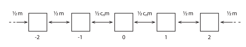
Figure 7: Jump rates of the random walk with an obstacle for $K=2$

Recall that $\left(\xi_{n}(t),t\geq 0\right)$ is a random walk on $E$ with jump rates given in (6), (7) (Figure 7) and that $X_{n}(t)=\frac{1}{\sqrt{n}}\xi_{n}(nt)$. Also recall that $d$ is a metric for Skorokhod convergence on compact time intervals (8).

Lemma 3.1.

The sequence $\{\left(X_{n}(t)\right)_{t\geq 0},n\geq 1\}$ is tight in $(\mathrm{D}\left(\mathbb{R}_{+},\mathbb{R}\right),d)$.

Let $\left(X_{\infty}(t)\right)_{t\geq 0}$ be an arbitrary limit point of this sequence (i.e. the limit of a converging subsequence).

Lemma 3.2.

$\left|X_{\infty}\right|$ is distributed as reflected Brownian motion with diffusion coefficient $m$.

Let $T_{0}=0$ and for $i\geq 0$,

$$T_{i+1}=\inf\{t>T_{i}:X_{\infty}(T_{i})X_{\infty}(t)<0\}.$$ (22)

Lemma 3.3.

$(L^{0}_{T_{i+1}}(X_{\infty})-L^{0}_{T_{i}}(X_{\infty}))_{i\geq 0}$ is a sequence of independent exponential random variables with parameter $\gamma$. This sequence is independent of $\left(\left|X_{\infty}(t)\right|\right)_{t\geq 0}$.

Proof of Theorem 1.

By Proposition 1.5, $X_{\infty}$ is characterized as (the projection on $\mathbb{R}$ of) partially reflected Brownian motion. Since the sequence $X_{n}$ is tight and has only one possible limit point in $\mathrm{D}\left(\mathbb{R}_{+},\mathbb{R}\right)$, it converges in distribution to partially reflected Brownian motion. ∎

The rest of this section is devoted to the proof of Lemmas 3.2, 3.3 and 3.1, in that order. In what follows, we assume, with a slight abuse of notation, that $\left(X_{n},n\geq 1\right)$ is a subsequence of the original sequence of processes which converges in distribution to $X_{\infty}$.

3.1 The absolute value of $X_{\infty}$

To prove that the absolute value of any possible limit point of $X_{n}$ is reflected Brownian motion, we write $\left|X_{n}\right|$ as the sum of a martingale term and a non-decreasing term. We then show that the martingale term converges to Brownian motion while the non-decreasing term converges to the opposite of the running minimum of this Brownian motion. The conclusion follows from a classical result on reflected Brownian motion [23, VI.2].

Set

$$\tilde{X}_{n}(t)=\left|X_{n}(t)\right|\mathds{1}_{\left\{\left|X_{n}(t)\right|\geq\frac{2}{\sqrt{n}}\right\}}$$

and, for $i\geq 0$,

$$\sigma_{0}^{n}=0, \tau_{i}^{n}=\inf\{t>\sigma_{i}^{n}:\left|X_{n}(t)\right|\leq\tfrac{1}{\sqrt{n}}\},$$

$$\sigma_{i+1}^{n}=\inf\{t>\tau_{i}^{n}:\left|X_{n}(t)\right|>\tfrac{1}{\sqrt{n}}\}.$$

The process $\tilde{X}_{n}$ can then be decomposed as follows [8]

$$\tilde{X}_{n}(t)=M_{n}(t)+L_{n}(t)-\sum_{i\geq 0}\left|X_{n}(\tau_{i}^{n})\right|\mathds{1}_{\left\{\tau_{i}^{n}\leq t<\sigma_{i+1}^{n}\right\}},$$ (23)

with

$$M_{n}(t)=\left|X_{n}(0)\right|+\int_{0}^{t}\mathds{1}_{\left\{\left|X_{n}(s)\right|>\frac{1}{\sqrt{n}}\right\}}d\left|X_{n}\right|(s)$$

and

$$L_{n}(t) =\sum_{i\geq 0}\left(\left|X_{n}(\sigma_{i+1}^{n})\right|-\left|X_{n}(\tau_{i}^{n})\right|\right)\mathds{1}_{\left\{\sigma_{i+1}^{n}\leq t\right\}}$$

$$=\frac{1}{\sqrt{n}}\sum_{i\geq 0}\mathds{1}_{\left\{\sigma_{i+1}^{n}\leq t\right\}}.$$ (24)

The term $M_{n}$ is a martingale, while $L_{n}$ counts the number of visits (in fact of exits) of $[-\frac{1}{\sqrt{n}},\frac{1}{\sqrt{n}}]$.

Define the running minimum $V_{n}(t)$ of the martingale part as

$$V_{n}(t)=\sup_{s\leq t}\left(\tfrac{2}{\sqrt{n}}-M_{n}(s)\right)^{+}$$ (25)

and note that $V_{n}$ first becomes positive when $M_{n}$ first reaches $\frac{1}{\sqrt{n}}$, i.e.

$$\inf\{t\geq 0:V_{n}(t)\geq\tfrac{1}{\sqrt{n}}\}=\inf\{t\geq 0:M_{n}(t)\leq\tfrac{1}{\sqrt{n}}\}.$$

Since up to that time the other terms on the right-hand-side of (23) are zero, we get

$$\inf\{t\geq 0:V_{n}(t)\geq\tfrac{1}{\sqrt{n}}\}=\tau_{0}^{n}.$$

The next time $V_{n}$ increases is

$$\inf\{t\geq 0:V_{n}(t)\geq\tfrac{2}{\sqrt{n}}\}=\inf\{t\geq 0:M_{n}(t)\leq 0\}.$$

By (23), this is also $\tau_{1}^{n}$. By induction,

$$V_{n}(t)=\frac{1}{\sqrt{n}}\sum_{i\geq 0}\mathds{1}_{\left\{\tau_{i}^{n}\leq t\right\}}.$$ (26)

This translates the fact that the excursions of $M_{n}$ above its running minimum are given by the excursions of $\left|X_{n}\right|$ above $\frac{1}{\sqrt{n}}$, see also Figure 8. Returning to (23), we have shown

$$\tilde{X}_{n}(t)=M_{n}(t)+V_{n}(t).$$ (27)

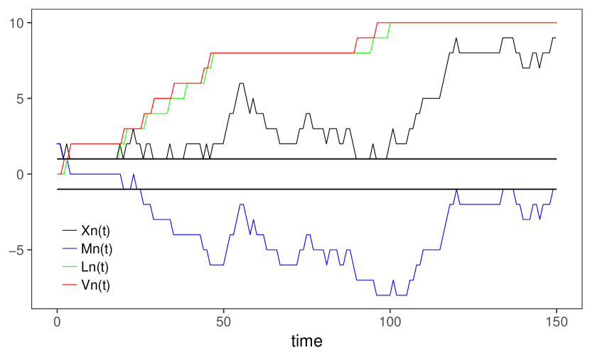
Figure 8: Decomposition of $X_{n}$

The black line shows a sample path of $X_{n}$ for $k=2$, $m=0.4$ and $c_{n}=0.1$. The blue line is $M_{n}$ while the green (resp. red) lines show $L_{n}$ (resp. $V_{n}$). We see that the excursions of $M_{n}$ above its running minimum are given by the excursions of $X_{n}$ outside $\{-1,1\}$.

Lemma 3.4.

The process $M_{n}$ converges in distribution in $(\mathrm{D}\left(\mathbb{R}_{+},\mathbb{R}\right),d_{sko})$ to $M_{\infty}$, a Brownian motion with variance parameter $m$ (started from $\left|X_{\infty}(0)\right|$).

We prove this lemma below, but let us first conclude the proof of Lemma 3.2.

Proof of Lemma 3.2.

Recall that we are already considering a subsequence along which $X_{n}$ converges to $X_{\infty}$. Passing to the limit in (27), we obtain

$$\left|X_{\infty}(t)\right|=M_{\infty}(t)+\sup_{s\leq t}\left(-M_{\infty}(s)\right)^{+}.$$

Setting

$$L(t)=\sup_{s\leq t}(-M_{\infty}(s))^{+},$$

we have by Lévy’s theorem [23, Theorem VI.2.3] that $(\left|X_{\infty}\right|,L)$ is distributed as $(\left|B\right|,L^{B})$, where $B$ is Brownian motion (with variance parameter $m$) and $L^{B}$ is its local time at zero. Hence $(\left|X_{\infty}(t)\right|,t\geq 0)$ is distributed as reflected Brownian motion and $(L(t),t\geq 0)$ is its local time at zero, i.e.

$$L^{0}_{t}(X_{\infty})=\sup_{s\leq t}(-M_{\infty}(s))^{+}.$$ (28)

∎

To show that $M_{n}$ converges to Brownian motion, we note that $M_{n}$ is a square integrable martingale with predictable variation

$$\langle M_{n}\rangle_{t}=m(t-\nu^{n}(t))$$

where

$$\nu^{n}(t)=\int_{0}^{t}\mathds{1}_{\left\{\left|X_{n}(s)\right|\leq\frac{1}{\sqrt{n}}\right\}}ds.$$ (29)

We prove the following lemma in Subsection 3.4.

Lemma 3.5.

For any $t\geq 0$, $\mathbb{E}\left[\nu^{n}(t)\right]=\mathcal{O}\left(\frac{1}{\sqrt{n}}\right)$.

The proof of Lemma 3.4 is then straightforward.

Proof of Lemma 3.4.

From (29) and Lemma 3.5, $\left\langle M_{n}\right\rangle_{t}\to mt$ in probability as $n\to\infty$. Moreover,

$$\sup_{t\geq 0}\left|M_{n}(t)-M_{n}(t^{-})\right|\leq\frac{1}{\sqrt{n}}$$

almost surely. Hence, for example from [21, Proposition II.1], $M_{n}$ converges to Brownian motion in distribution in $\mathrm{D}\left({[0,T]},\mathbb{R}\right)$ for all $T>0$. ∎

In passing, we have proved the following lemma.

Lemma 3.6.

$\left(X_{n},L_{n}\right)\overset{d}{\underset{n\to\infty}{\longrightarrow}}\left(X_{\infty},L^{0}(X_{\infty})\right)$

Proof.

From (25) and the convergence of $M_{n}$, it is clear that the pair of processes $(X_{n},V_{n})$ converges in distribution in $\mathrm{D}\left({[0,T]},\mathbb{R}^{2}\right)$ to $(X_{\infty},L_{\infty})$, where

$$L_{\infty}(t)=\sup_{s\leq t}(-M_{\infty}(s))^{+}.$$

Furthermore, from (26) and (24), we have for all $t\geq 0$

$$\left|L_{n}(t)-V_{n}(t)\right|\leq\frac{1}{\sqrt{n}}.$$

As a result the pair $(X_{n},L_{n})$ converges in distribution in $\mathrm{D}\left({[0,T]},\mathbb{R}^{2}\right)$ to $(X_{\infty},L_{\infty})$. We conclude the proof by noting that $L_{\infty}(t)=L^{0}(X_{\infty})$, as shown in (28). ∎

3.2 Local time accumulated between crossings

To prove that the local time accumulated by $X_{\infty}$ at the origin between crossings is a sequence of exponential variables, we show that the number of visits of the random walk $X_{n}$ to $[-\frac{1}{\sqrt{n}},\frac{1}{\sqrt{n}}]$ before the first time it reaches $-\frac{2}{\sqrt{n}}$ is a geometric random variable.

Let $(T_{i}^{n},i\geq 0)$ be the sequence of crossing times of $[-1/\sqrt{n},1/\sqrt{n}]$ by $X_{n}$, i.e. for $n\geq 0$, set $T_{0}^{n}=0$ and

$$T_{i+1}^{n}=\inf\{t>T_{i}^{n}:\operatorname{sign}(X_{n}(T_{i}^{n}))X_{n}(t)<-\tfrac{1}{\sqrt{n}}\}.$$

Recall also the definition of $(T_{i},i\geq 0)$ in (22).

Lemma 3.7.

As $n$ tends to infinity,

$$\left(X_{n},L_{n},\left(T_{i}^{n}\right)_{i\geq 0}\right)\overset{d}{\underset{n\to\infty}{\longrightarrow}}\left(X_{\infty},L^{0}(X_{\infty}),\left(T_{i}\right)_{i\geq 0}\right)$$

in $\mathrm{D}\left([0,T]^{2},\mathbb{R}^{2}\right)\times\mathbb{R}^{\mathbb{N}}$.

The proof of Lemma 3.7 is given in Subsection 3.5.

Proof of Lemma 3.3.

Let $Y_{n}$ be the number of visits to $[-\frac{1}{\sqrt{n}},\frac{1}{\sqrt{n}}]$ up to the first crossing time,

$$Y_{n}=\sum_{i\geq 1}\mathds{1}_{\left\{\sigma_{i}^{n}\leq T_{1}^{n}\right\}}.$$

By the Markov property, $Y_{n}$ is a geometric random variable with parameter

$$p_{n}=\mathbb{P}_{\tfrac{1}{\sqrt{n}}}\left(X_{n}(\sigma_{1}^{n})=-\tfrac{2}{\sqrt{n}}\right).$$

For $K=2$, $p_{n}=\frac{c_{n}}{2(1+c_{n})}$ (and in the general case, $p_{n}\sim\frac{c_{n}}{K}$ as $n\to\infty$). Since $\frac{\sqrt{n}}{2}c_{n}\to\gamma\in(0,\infty)$,

$$L_{n}(T_{1}^{n})=\frac{1}{\sqrt{n}}Y_{n}$$

converges in distribution to an exponential random variable with parameter $\gamma$. Set $E^{n}_{i}=L_{n}(T^{n}_{i+1})-L_{n}(T^{n}_{i})$. The random variables $E_{0}^{n},E_{1}^{n},\ldots$ are independent and identically distributed by the strong Markov property and by symmetry. As a result, $\left(E^{n}_{i}\right)_{i\geq 0}$ converges in distribution as $n$ tends to infinity to a sequence $\left(E_{i}\right)_{i\geq 0}$ of independent and identically distributed exponential random variables with parameter $\gamma$. By Lemma 3.7, this limit coincides with $(L^{0}_{T_{i+1}}(X_{\infty})-L^{0}_{T_{i}}(X_{\infty}))_{i\geq 0}$ (also note that $t\mapsto L^{0}_{t}(X_{\infty})$ is continuous almost surely).

We would like to show that the sequence $\left(E_{i}^{n}\right)_{i\geq 0}$ is independent of $\tilde{X}_{n}$, but this fails when $K\geq 2$. To circumvent this issue, we tweak $\tilde{X}_{n}$ so that it “forgets” the amount of time $X_{n}$ spends in $[-\frac{1}{\sqrt{n}},\frac{1}{\sqrt{n}}]$. We do this via a time change. Set

$$\delta^{n}_{i}=\inf\{t>\tau_{i}^{n}:X_{n}(t)\neq X_{n}(t^{-})\}$$

and

$$\theta^{n}(t)=\inf\left\{\theta>0:\int_{0}^{\theta}\sum_{i\geq 0}\mathds{1}_{\left\{s\notin[\delta_{i}^{n},\sigma_{i+1}^{n}[\right\}}ds>t\right\}.$$

Then $(\tilde{X}_{n}(\theta^{n}(t)),t\geq 0)$ and $(L_{n}(T_{i+1}^{n})-L_{n}(T_{i}^{n}))_{i\geq 0}$ are independent. Furthermore, for $t\geq 0$,

$$\left|\int_{0}^{t}\sum_{i\geq 0}\mathds{1}_{\left\{s\notin[\delta_{i}^{n},\sigma_{i+1}^{n}[\right\}}ds-t\right|\leq\nu^{n}(t).$$

Moreover $t\mapsto\nu^{n}(t)$ is nondecreasing, hence, by Lemma 3.5, $(\nu^{n}(t),t\geq 0)$ converges to 0 uniformly on compact sets in $L^{1}$. It follows that $\theta^{n}(t)\to t$ as $n\to\infty$ uniformly on compact sets in probability. As a result, $\tilde{X}_{n}\circ\theta^{n}$ converges in the Skorokhod topology to $\left|X_{\infty}\right|$ (also in probability). We can thus conclude that $(L^{0}_{T_{i+1}}(X_{\infty})-L^{0}_{T_{i}}(X_{\infty}))_{i\geq 0}$ is independent of $\left|X_{\infty}\right|$. ∎

3.3 Tightness

Proof of Lemma 3.1.

Tightness of the sequence $X_{n}$ follows from the convergence in distribution of $M_{n}$ (recall the decomposition (23)). Reasoning as in [8] (Proof of Lemma 2.1), we show below that for any $\delta>0$,

$$\sup_{\left|s-t\right|<\delta}\left|X_{n}(t)-X_{n}(s)\right|\leq\tfrac{3}{\sqrt{n}}+2\sup_{\left|s-t\right|<\delta}\left|M_{n}(t)-M_{n}(s)\right|.$$ (30)

We can thus write, for $T>0$ and $\varepsilon>0$

$$\lim_{\delta\downarrow 0}\limsup_{n\to\infty}\mathbb{P}\Bigg{(}\sup_{\begin{subarray}{c}\left|t-s\right|<\delta\\ s,t\in[0,T]\end{subarray}}\left|X_{n}(s)-X_{n}(t)\right|>\varepsilon\Bigg{)}\\ \leq\lim_{\delta\downarrow 0}\limsup_{n\to\infty}\mathbb{P}\Bigg{(}\tfrac{3}{\sqrt{n}}+2\sup_{\begin{subarray}{c}\left|t-s\right|<\delta\\ s,t\in[0,T]\end{subarray}}\left|M_{n}(t)-M_{n}(s)\right|>\varepsilon\Bigg{)}.$$

The right-hand-side is zero because the sequence $M_{n}$ converges in distribution in the space $\mathrm{D}\left({[0,T]},\mathbb{R}\right)$, and tightness of $X_{n}$ in $\mathrm{D}\left({[0,T]},\mathbb{R}\right)$ follows [3, Theorem 7.3]. Since $X_{n}$ is tight in $\mathrm{D}\left({[0,T]},\mathbb{R}\right)$ for all $T>0$, it is tight in $(\mathrm{D}\left(\mathbb{R}_{+},\mathbb{R}\right),d)$.

Let us now prove (30). Fix $0\leq s\leq t$. If $\left|X_{n}(u)\right|>\frac{1}{\sqrt{n}}$ for all $u\in[s,t]$, then

$$X_{n}(t)-X_{n}(s)=M_{n}(t)-M_{n}(s).$$

Otherwise, let

$$\alpha =\inf\{u>s:\left|X_{n}(u)\right|\leq\tfrac{1}{\sqrt{n}}\},$$

$$\beta =\sup\{u<t:\left|X_{n}(u)\right|\leq\tfrac{1}{\sqrt{n}}\},$$

and note that

$$\left|X_{n}(t)-X_{n}(s)\right| \leq\left|X_{n}(t)-X_{n}(\beta)\right|+\left|X_{n}(\beta)-X_{n}(\alpha)\right|+\left|X_{n}(\alpha)-X_{n}(s)\right|$$

$$\leq\tfrac{3}{\sqrt{n}}+\left|M_{n}(t)-M_{n}(\beta)\right|+\left|M_{n}(s)-M_{n}(\alpha)\right|.$$

Inequality (30) thus holds and the proof of Lemma 3.1 is complete. ∎

3.4 Occupation time of the barrier

Proof of Lemma 3.5.

The bound on the expected time spent inside $[-\frac{1}{\sqrt{n}},\tfrac{1}{\sqrt{n}}]$ follows after showing that the expected length of a visit in this set is of order $\frac{1}{n}$ while the expected number of those visits is of order $\sqrt{n}$. By the definition of $\nu^{n}(t)$,

$$\nu^{n}(t) =\sum_{i\geq 0}\left(\sigma_{i+1}^{n}\wedge t-\tau_{i}^{n}\wedge t\right)$$

$$\leq\sum_{i\geq 0}\left(\sigma_{i+1}^{n}-\tau_{i}^{n}\right)\mathds{1}_{\left\{\tau_{i}^{n}\leq t\right\}}.$$

By the strong Markov property,

$$\mathbb{E}\left[\nu^{n}(t)\right]\leq\mathbb{E}\left[\sum_{i\geq 0}h^{n}(X_{n}(\tau_{i}^{n}))\mathds{1}_{\left\{\tau_{i}^{n}\leq t\right\}}\right]$$

where $h^{n}(x)=\mathbb{E}_{x}\left[\inf\{t>0:\left|X_{n}(t)\right|>\frac{1}{\sqrt{n}}\}\right]$. By the Markov property, for $i\in\{-1,0,1\}$,

$$n\sum_{j\in E}q_{n}(i,j)\left(h^{n}(j/\sqrt{n})-h^{n}(i/\sqrt{n})\right)=-1.$$

Also $h^{n}(x)=0$ when $\left|x\right|>\frac{1}{\sqrt{n}}$. Solving these equations for $K=2$ yields

$$h^{n}\left(\pm\tfrac{1}{\sqrt{n}}\right)=\frac{3}{mn}, h^{n}(0)=\frac{3}{mn}+\frac{1}{c_{n}mn}.$$

(In the general case, $h^{n}\left(\lfloor\frac{K+1}{2}\rfloor/\sqrt{n}\right)=\frac{K+1}{mn}$.) For $i\geq 1$, $X_{n}(\tau_{i}^{n})=\pm\frac{1}{\sqrt{n}}$, hence

$$\mathbb{E}\left[\nu^{n}(t)\right]\leq\frac{1}{c_{n}mn}+\frac{3}{mn}\mathbb{E}\left[\sum_{i\geq 0}\mathds{1}_{\left\{\tau_{i}^{n}\leq t\right\}}\right].$$

But the number of visits of $X_{n}$ to $[-\frac{1}{\sqrt{n}},\tfrac{1}{\sqrt{n}}]$ before time $t$ is less than the number of excursions outside $[-\frac{1}{\sqrt{n}},\tfrac{1}{\sqrt{n}}]$ before the first excursion of length longer than $t$. By the Markov property, the latter is a geometric random variable with parameter

$$\mathbb{P}_{\tfrac{2}{\sqrt{n}}}\left(\tau_{0}^{n}>t\right).$$

But, for $t>0$, there exists $c\in(0,\infty)$ such that [11, Proposition 4.2.4]

$$\lim_{n\to\infty}\sqrt{n}\mathbb{P}_{\tfrac{2}{\sqrt{n}}}\left(\tau_{0}^{n}>t\right)=c.$$

Hence, since $\sqrt{n}c_{n}\to K\gamma\in(0,\infty)$,

$$\mathbb{E}\left[\nu^{n}(t)\right]\leq\frac{1}{c_{n}nm}+\frac{3}{m\sqrt{n}}\left(\sqrt{n}\mathbb{P}_{\tfrac{2}{\sqrt{n}}}\left(\tau_{0}^{n}>t\right)\right)^{-1}=\mathcal{O}\left(\frac{1}{\sqrt{n}}\right).$$

This concludes the proof of Lemma 3.5. ∎

3.5 Convergence of the crossing times

Proof of Lemma 3.7.

From Lemma 3.6, we already know that

$$(X_{n},L_{n})\overset{d}{\underset{n\to\infty}{\longrightarrow}}(X_{\infty},L^{0}(X_{\infty})).$$

Furthermore, for all $i\geq 0$,

$$T_{i}^{n}=L_{n}^{-1}\left(\sum_{k=1}^{i}E_{k}^{n}\right),$$

where $t\mapsto L_{n}^{-1}(t)$ is the right continuous inverse of $L_{n}$. Since $\left(E_{i}^{n}\right)_{i\geq 0}$ converges in distribution to $\left(E_{i}\right)_{i\geq 0}$ and $L_{n}$ converges in distribution to $L^{0}(X_{\infty})$, the sequence $\left(T_{i}^{n}\right)_{n\geq 1}$ is tight in $\mathbb{R}$ for all $i\geq 0$.

As a result the sequence of random variables $(X_{n},L_{n},\left(T_{i}^{n}\right)_{i\geq 0})$ is tight in $\mathrm{D}([0,T]^{2}$, $\mathbb{R}^{2})\times\mathbb{R}^{\mathbb{N}}$, where this space is endowed with the product topology. Let $(X_{\infty}$, $L^{0}(X_{\infty})$, $(\tilde{T}_{i})_{i\geq 0})$ be a possible limit point of this subsequence. By the Skorokhod embedding theorem, we can assume that there exists (a version of) a subsequence which converges to (a version of) this limit point almost surely. For ease of notation we denote this subsequence by $(X_{n},L_{n},\left(T_{i}^{n}\right)_{i\geq 0})$.

Let $\mathcal{N}\subset\Omega$ be the negligible set on which this convergence fails, and suppose that there exists $\omega\in\Omega\setminus\mathcal{N}$ such that $\tilde{T}_{1}(\omega)<T_{1}(\omega)$. We show that for this to happen, one of two very improbable things must occur: either $\tilde{T}_{1}(\omega)=\tilde{T}_{2}(\omega)$ (but remember that $L_{n}(T^{n}_{2})-L_{n}(T^{n}_{1})$ is asymptotically exponentially distributed) or $X_{\infty}$ must remain equal to zero for a positive amount of time after $\tilde{T}_{1}$.

Assume without loss of generality that $X_{\infty}(0)>0$ and that $X_{n}(0)>0$ for all $n\geq 1$. Then take $\varepsilon>0$ such that $\tilde{T}_{1}+\varepsilon<T_{1}$ ($\omega$ is kept fixed in the remainder of the proof). Since $X_{n}\Rightarrow X_{\infty}$,

$$\inf\{X_{n}(s),T_{1}^{n}\leq s\leq T_{1}^{n}+\varepsilon\}\underset{n\to\infty}{\longrightarrow}\inf\{X_{\infty}(s),\tilde{T}_{1}\leq s\leq\tilde{T}_{1}+\varepsilon\}.$$

Since $X_{\infty}(s)\geq 0$ for $s<T_{1}$, the right-hand-side is non-negative while the left-hand-side is non-positive because $X_{n}(T_{1}^{n})=-\frac{2}{\sqrt{n}}$. As a result

$$\lim_{n\to\infty}\inf\{X_{n}(s),T_{1}^{n}\leq s\leq T_{1}^{n}+\varepsilon\}=0.$$

Also note that

$$\sup\{\left|X_{n}(s)\right|,T_{1}^{n}\leq s\leq T_{2}^{n}\wedge(T_{1}^{n}+\varepsilon)\}\leq\left|\inf\{X_{n}(s),T_{1}^{n}\leq s\leq T_{1}^{n}+\varepsilon\}\right|.$$

Moreover the left-hand-side converges to

$$\sup\{\left|X_{\infty}(s)\right|,\tilde{T}_{1}\leq s\leq\tilde{T}_{2}\wedge(\tilde{T}_{1}+\varepsilon)\}.$$

The latter must then be zero. Hence either $\tilde{T}_{1}=\tilde{T}_{2}$ or there exists $\eta>0$ such that $\left|X_{\infty}(s)\right|=0$ for all $\tilde{T}_{1}\leq s\leq\tilde{T}_{1}+\eta$. Since $L_{n}(T_{1}^{n})-L_{n}(T_{2}^{n})$ converges to an exponential random variable with parameter $\gamma\in(0,\infty)$ and $\left|X_{\infty}\right|$ is distributed as reflected Brownian motion, both these events have probability zero.

Suppose now that $\tilde{T}_{1}(\omega)>T_{1}(\omega)$ for some $\omega\in\Omega\setminus\mathcal{N}$. By the definition of $T_{1}$, there exists $t\in(T_{1},\tilde{T}_{1})$ such that $X_{\infty}(t)<0$. Since $T_{1}\to\tilde{T}_{1}>t$, there exists $n_{0}$ large enough that $T_{1}^{n}>t$ for all $n\geq n_{0}$. Then for all $n\geq n_{0}$, $X_{n}(t)\geq-\frac{1}{\sqrt{n}}$, but at the same time $X_{n}(t)\to X_{\infty}(t)<0$, leading to a contradiction.

We have thus shown that $\tilde{T}_{1}=T_{1}$ almost surely. By induction one shows that $\tilde{T}_{i}=T_{i}$ almost surely for all $i\geq 0$. It follows that $(X_{\infty},L_{\infty},\left(T_{i}\right)_{i\geq 0})$ is the only possible limit point of the sequence $(X_{n},L_{n},\left(T_{i}^{n}\right)_{i\geq 0})$. Together with the tightness of this sequence, this concludes the proof of Lemma 3.7. ∎

References

- ABT+ [11] Thilanka Appuhamillage, Vrushali Bokil, Enrique Thomann, Edward Waymire, and Brian Wood. Occupation and local times for skew Brownian motion with applications to dispersion across an interface. The Annals of Applied Probability, 21(1):183–214, 2011.
- Bar [08] Nick H. Barton. The effect of a barrier to gene flow on patterns of geographic variation. Genetics research, 90(01):139–149, 2008.
- Bil [99] Patrick Billingsley. Convergence of Probability Measures. Wiley Series in Probability and Statistics. John Wiley & Sons, Inc., New York, second edition, 1999.
- EK [86] Stewart N. Ethier and Thomas G. Kurtz. Markov Processes: Characterization and Convergence. John Wiley & Sons, Inc., New York, 1986.
- Gre [06] Denis S. Grebenkov. Partially reflected Brownian motion: A stochastic approach to transport phenomena. In Focus on Probability Theory, pages 135–169. Nova Sci. Publ., New York, 2006.
- GVNL [14] Denis S. Grebenkov, Dang Van Nguyen, and Jing-Rebecca Li. Exploring diffusion across permeable barriers at high gradients. I. Narrow pulse approximation. Journal of Magnetic Resonance, 248:153–163, November 2014.
- Har [85] J. Harrison. Brownian Motion and Stochastic Flow Systems. 1985.
- IP [16] Alexander Iksanov and Andrey Pilipenko. A functional limit theorem for locally perturbed random walks. Probability and Mathematical Statistics, 36(2):353–368, 2016.
- Kni [71] Frank B. Knight. A reduction of continuous square-integrable martingales to Brownian motion. Lecture notes in Math, 190:19–31, 1971.
- Lej [16] Antoine Lejay. The snapping out Brownian motion. The Annals of Applied Probability, 26(3):1727–1742, 2016.
- LL [10] Gregory F. Lawler and Vlada Limic. Random Walk: A Modern Introduction, volume 123 of Cambridge Studies in Advanced Mathematics. Cambridge University Press, Cambridge, 2010.
- MP [16] Vidyadhar Mandrekar and Andrey Pilipenko. On a Brownian motion with a hard membrane. Statistics & Probability Letters, 113:62–70, June 2016.
- Nag [76] Thomas Nagylaki. Clines with Variable Migration. Genetics, 83(4):867–886, 1976.
- Nag [88] Thomas Nagylaki. The influence of spatial inhomogeneities on neutral models of geographical variation. I. Formulation. Theoretical Population Biology, 33(3):291–310, 1988.
- [15] Thomas Nagylaki. Clines with partial panmixia. Theoretical population biology, 81(1):45–68, 2012.
- [16] Thomas Nagylaki. Clines with partial panmixia in an unbounded unidimensional habitat. Theoretical population biology, 82(1):22–28, 2012.
- Nag [16] Thomas Nagylaki. Clines with partial panmixia across a geographical barrier. Theoretical Population Biology, 109:28–43, June 2016.
- NFJH [11] Dmitry S. Novikov, Els Fieremans, Jens H. Jensen, and Joseph A. Helpern. Random walks with barriers. Nature physics, 7(6):508–514, 2011.
- NKD [93] T. Nagylaki, P. T. Keenan, and T. F. Dupont. The Influence of Spatial Inhomogeneities on Neutral Models of Geographical Variation III. Migration across a Geographical Barrier. Theoretical Population Biology, 43(2):217–249, April 1993.
- NZ [16] Thomas Nagylaki and Kai Zeng. Clines with partial panmixia across a geographical barrier in an environmental pocket. Theoretical Population Biology, 110:1–11, August 2016.
- Reb [80] Rolando Rebolledo. Central limit theorems for local martingales. Zeitschrift für Wahrscheinlichkeitstheorie und Verwandte Gebiete, 51(3):269–286, 1980.
- RKFB [18] Harald Ringbauer, Alexander Kolesnikov, David L. Field, and Nicholas H. Barton. Estimating barriers to gene flow from distorted isolation by distance patterns. Genetics, pages genetics–300638, 2018.
- RY [13] Daniel Revuz and Marc Yor. Continuous Martingales and Brownian Motion, volume 293. Springer Science & Business Media, 2013.
- SB [89] Montgomery Slatkin and Nick H. Barton. A Comparison of Three Indirect Methods for Estimating Average Levels of Gene Flow. Evolution, 43(7):1349–1368, 1989.
- SK [91] S. E. Shreve and I. Karatzas. Brownian Motion and Stochastic Calculus, volume 113. Springer, 1991.
- Sko [61] A. Skorokhod. Stochastic Equations for Diffusion Processes in a Bounded Region. Theory of Probability & Its Applications, 6(3):264–274, January 1961.
- Sla [73] Montgomery Slatkin. Gene flow and selection in a cline. Genetics, 75(4):733–756, 1973.
- SQH+ [03] H. Su, L. J. Qu, K. He, Z. Zhang, J. Wang, Z. Chen, and H. Gu. The Great Wall of China: A physical barrier to gene flow? Heredity, 90(3):212–219, 2003.
- Wri [43] Sewall Wright. Isolation by distance. Genetics, 28(2):114, 1943.