Analysis of the U.S. Patient Referral Network

Abstract

In this paper we analyze the US Patient Referral Network (also called the Shared Patient Network) and various subnetworks for the years 2009–2015. In these networks two physicians are linked if a patient encounters both of them within a specified time-interval, according to the data made available by the Centers for Medicare and Medicaid Services. We find power law distributions on most state-level data as well as a core-periphery structure. On a national and state level, we discover a so-called small-world structure as well as a “gravity law” of the type found in some large-scale economic networks. Some physicians play the role of hubs for interstate referral. Strong correlations between certain network statistics with healthcare system statistics at both the state and national levels are discovered. The patterns in the referral network evinced using several statistical analyses involving key metrics derived from the network illustrate the potential for using network analysis to provide new insights into the healthcare system and opportunities or mechanisms for catalyzing improvements.

Keywords: Generative model; Hierarchical modeling; Network science; Physician network; Shared patient network; Social network analysis

1 Introduction and Background

A well-designed healthcare system is a key component of a working society, and the ability for information and resources to flow efficiently in such a system is crucial to its efficacy. Inefficient communication in the United States healthcare system oftentimes results in ineffective care coordination. [47] Referrals are one of the most common and important forms of primary-specialty care communication. The existence of a shared patient relationship between physicians likely means there exists professional, information-sharing relationships between the two. [2, 41] Physicians decide to refer patients to other physicians in other hospitals for a multitude of reasons ranging from the need for specialization to addressing problems of overcrowding. The top three reasons for a primary care physician to refer a patient to a specialist are (1) seeking advice on a diagnosis or treatment (52.1%), (2) requesting surgical management (37.8%), and (3) asking the specialist to directly manage the patient (25.1%). [14] A physician’s decision to refer (or not refer) a patient is important in determining cost and quality of care. [4] See also. [5, 6]

The referral of a patient by physician $A$ to physician $B$ is naturally represented as a directed edge from a network node labeled $A$ to a node labeled $B$, forming a directed network (possibly weighted by the number of such referrals). [2] (See https://blog.pokitdok.com/physician-co-occurrence-graphs-part-1-of-2/ for visualizations of physician “ego networks”: network diagrams illustrating all referral relationships that include a single particular physician.) In this paper we analyze the structure of an important physician network and in this context introduce a number of novel concepts from the network science and social networks fields; drawing together methods from both of these two growing but surprisingly distinct fields is an important and novel feature of this work that is hoped will catalyze their combined use across the statistical sciences as applied to healthcare related networks.

In particular, in this paper we use data from the Centers for Medicare and Medicaid Services (see [9, 10]) that is freely available and therefore among (often closely held) healthcare data sets is uniquely amenable to enabling reproducible research. The key data element is the counts of patients encountered by one physician and then another physician within an interval of time (we use 30 days). The networks constructed from physicians’ caring for the same patients have been variously described as a referral network, a collaboration network, an informal physician network, and a patient-sharing network. It reflects collaboration, coordination, communication channels, diffusion of information, and possibly diffusion of medical innovations. [41, 4, 5, 6, 20, 24] Although counts of shared patients do not necessarily represent formal referrals from one physician to the other, for ease of terminology we take referral to mean the event that a patient encounters the first physician followed by the second within 30 days.

One motivation for studying physician networks stems from reported associations of collaboration with effectiveness in delivering health services and its recognition as a catalyst to improved patient outcomes. [37, 42] For example, associations have been found between collaboration and hospital length of stay, lower re-admission rates, lower hospital cost, lower death rate, and higher satisfaction. [11, 17, 35, 39] A multi-level regression model [40] has previously been used to study the relationship between patient-care networks and healthcare outcomes. Our work differs from this in that we summarize networks using a broader range of metrics, including many from the field of network science and even measures such as gravity that may be unfamiliar to social network analysts, and use state-level healthcare metrics as opposed to patient-level metrics. Network analysis has the potential to differentiate physicians’ local network structure and network positions, reflecting different structures of collaboration, and determining if these explain variation in important health outcomes. [7] In so doing, network analysis can identify favorable network structure and provide a recipe for organizing healthcare in a more optimal way.

Prior studies have not provided guidance about the network structure of effective healthcare collaboration, i.e., they have not been able to articulate what types of structure may be more conducive for the administration of effective healthcare. Nor have they prescribed how individual healthcare professionals should develop relationships over time for better outcomes. [41] Yet, the formation of physician networks from patient encounters as reported in health insurance claims data is becoming increasingly common. To date, the focus has been on the production of descriptive measures of the networks, including: density, degree, centrality (betweenness, eigenvector, Bonacich), strength (number of shared patients), clustering coefficient, assortativity, reciprocity, transitivity, cyclic triads, network distance and the positioning of physicians within the network (e.g., [20, 24, 22, 23]). Much less focus has been paid to developing and testing generative models able to capture the change in the network across time. Furthermore, the complexity of network data has often been overlooked and network statistics are often reported without statistical tests to determine if the feature in question is significantly different from what would be expected under a simple generative model of the network representing a meaningful null hypothesis.

Another overlooked issue is the impact of artificially imposed boundary definitions on the network. We are uniquely positioned to investigate boundary effects given that our data covers the complete US referral network. This allows us to assess whether analyses of geographically-defined sub-networks (e.g., state networks) and derived structural assessments are sensitive to the definition of the boundary and thus may distort the relationship of the network to important health variables.

A core area of research in health services research is the examination of the volume-outcome hypothesis under which physicians and hospitals who perform more procedures get better at them as reflected in their patient outcomes. A network-centric point of view suggests natural generalizations. If increased volume leads to better outcomes one might think that in a network context that the most well functioning healthcare organizations or regions will be those with the strongest physician network ties. However, the weak ties hypothesis [15, 16] may imply a more complex story. Perhaps, rare referral pathways are the most crucial elements of the physician network. The analysis herein may be useful for exploring such hypotheses.

We analyze the structure of patient referral networks at both national and state levels. We evaluate both macro (global) and micro (local configuration or actor specific) network features, describe the network in static and dynamic terms, and test against and for generative models such as the random network, the small-world, and power-law network, while also measuring the degree to which structural phenomena such as high core-periphery tendency are evident in the referral network. With longitudinal referral data between 2009 and 2015, we also are able to study changes in the connectivity of the healthcare system. Moreover, we incorporate healthcare metrics for the fifty states and apply regression models to estimate the relationship of state-level network features to them. The main contributions of our work are:

• Novel application of combined network science and social network methods to the referral network of all US physicians caring for patients on Medicare. The results show several revealing patterns in network structure.

• Evaluation of whether national-level patterns and phenomena reproduce at the state-level and whether state-level, or other sub-network analyses may yield misleading results.

• Estimation of multi-level regression models that extract the portion of the association between the network features and state level healthcare attributes that is independent of other predictors in a multiple regression framework.

It is important to note that the conclusions we draw are specific to the data source – that is the population of patients using Medicare and the physicians who care for them. Nevertheless, even with that caveat, the novelty of our work is seen in the scale of analysis, the consideration of network metrics relevant to the question of whether particular generative stories for the network are plausible, and the investigation of whether both macro (whole network) and micro (actor specific) network metrics are associated with various healthcare and health litigation metrics. Previous research on patient referral networks considers different questions and with not nearly as complete or expansive a network as that considered herein. For example, Lee [21] focuses on a single hospital in Orange County, CA, showing a tendency of physicians there to share patients with physicians at great distance (the “weak ties hypothesis”). Barnett et al. study primary care physician referral patterns using logistic regression [4] and find a relationship between patient sharing and at least one of the physicians reporting a professional relationships between them (via self-reported survey response), thereby providing some validation for using health insurance claims to identify patient-physician encounters to develop subsequently physician networks. This patient-sharing basis for developing the network is the same as that used herein. Landon et al. [20] consider the patient referral network at the HRR level and show the variation in network features at this scale, while discussing the factors related to building the referral connection between physicians. In an important longitudinal investigation, Barnett [6] finds changes in trends around referrals between physicians in 1999–2009 and that the structure of an HRR shared patient network has significant associations with costs and intensity of care. Landon et al.  [20] examines how physicians’ professional networks differ across geographic regions. Referral networks can also be viewed as collaboration networks for physicians, making relevant the large body of work on collaboration networks (see e.g., [28]) and networks of business relationship such as “interlocking corporate boards”. [34]

The organization of the remainder of the paper is as follows. Section 2 describes the data and outlines the methods and analyses used in this paper. Section 3 presents our findings on the structural metrics of the referral networks. In Section 4 we relate these to healthcare statistics. Finally, Section 5 concludes by describing the potential of a combined approach encompassing generative and empirical models involving networks and their key features to provide insights into the US healthcare system that could suggest pathways toward improving its organization.

2 Materials, Notation, and Methodology

2.1 Materials

Data. We used the CMS patient referral data set [9] to form a physician network of the US healthcare system. Datasets are available for the years 2009–2015, measuring the number of patients encountered by one physician and then the other physician within 30-, 60-, 90-, and 180-day interval per year, so the referrals are derived with a threshold (e.g. 30-day) over a given year. The referral dataset includes two parts, the referral records between two physicians and the attributes of the physicians. Sharing (referral) occurs when the same patient is recorded as having been treated by two different physicians in a given time period. The dates of treatment are timestamps. In this paper, we choose the 30-day interval referral dataset, because it judges the existence of direct referrals between two physicians with the most stringent criteria. For example, if a patient visits physician A two months after a visit to physician B the record will not be counted in the 30-day dataset, but will be counted in the datasets with longer time window. A referral dataset with longer interval will include more referrals, so some patterns (e.g., “small-world” below) in the referral networks found for the 30-day interval dataset would only be strengthened for the more expansive dataset. Physicians are listed according to National Provider Identification (NPI) number. (There are $4,332,951$ physicians in the NPI dataset.) A full data description can be found online. [10] In addition, the National Bureau of Economic Research “National Provider Identification number by state” data was used to attribute each physician in each year to a state based on their NPI. Some physicians are registered in several states. We label a physician according to the state in which the physician makes the most referrals. Table 1 shows the number of 30-day-interval referral records for the years 2009-2015. Notice that there are fewer referrals in 2015 due to the fact that data was only obtained for 7 months of the year (the end-date of the data is 10/1/2015 and so the last date for a first visit under which a full 60-days is available for a second visit is 7/31/2015). Accordingly, we expect a reduction in the average number of referrals between two physicians in 2015 compared to the earlier years. (This may mean that network features in 2015 might not be comparable to those in 2009-2014.)

Networks of interest. To produce a network description of the data, each physician is a node in the network. An edge (link) between two nodes (physicians) reflects the existence of the patient referral, and can be weighted by the number of referrals or simply given a weight of $1$ to indicate the connection. The edge can be directed (indicating time – referral) or undirected (encoding only sharing).

Given this data we form three kinds of networks (over a given time period): (1) The National Patient Referral Network includes all physicians in the US who have either made or received referrals over the period; (2) The (50) State Patient Referral Networks wherein for state $S$, the node set is all physicians who are either labeled as physicians in state $S$ or have either made referrals to or received referrals from physicians labeled with state $S$ over the period; The (50) Intrastate Patient Referral Networks is a subnetwork of the State Patient Referral Networks and requires that both physicians in a referral be labeled as in state $S$. The node set for state $S$ is all physicians with NPI numbers in state $S$ who have either made or received referrals over the given period. In network terminology the State Patient Referral Network would be called the subnetwork induced by the Intrastate Patient Referral Network. The three kinds of networks are nested as

$$\begin{array}[]{c}\mbox{National Patient Referral Network}\cr\cup\cr\mbox{(Induced) State Patient Referral Network of State }S\cr\cup\cr\mbox{Intrastate State Patient Referral Network of State }S\end{array}$$

for each state $S$. Each of these networks can be studied as simple undirected or directed networks, weighted or unweighted (wherein the weights are the number of referrals). These networks are also called Shared Patient Networks.

2.2 Macro-level and small scale network structures

There are still a relatively small number of well-defined – or at least named – macro-level structures. Three of interest are the random, small world and core-periphery networks. We first introduce these and then describe various small scale or local network structures of interest whose prominence in the network can be tested against assumed models of macro-level structure.

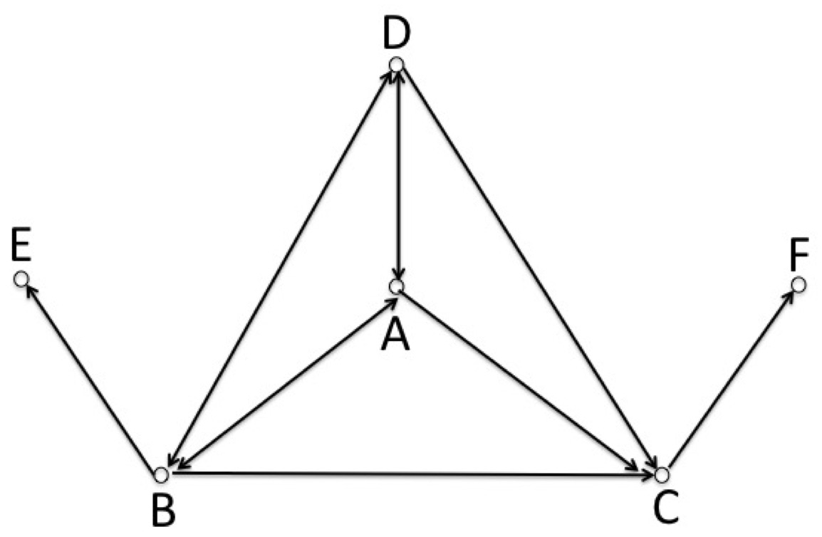
Figure 1: An illustrative directed network. The nodes A, B, C, D, E, and F represent different physicians. The arrow of an edge points from a referring physician to a referred physician (who accepts the patient referral).

• Erdós-Renyi (ER) random network – is the traditional null model against which network structure is measured. The ER network on a fixed number $n$ of nodes is constructed by independently joining any two vertices with an (undirected) edge with fixed probability $p$. [13] It is easy to see that the expected degree for any vertex in such a network is $\mu=(n-1)p$, and that the degree distribution follows the binomial $B(n-1,p)$, which for large $n$ is well approximated by a Poisson distribution with mean $\mu$. Ascribing structure to a network derives from showing that in various important parameters it differs from the comparable ER network with probability $p=\mu/(n-1)$ where $\mu$ is the average degree of the actors in the network.

• Small world network – is defined as a network with greater than expected local connectivity and average path length [44] smaller than expected in a comparable ER random network. More rigorously, a network is a small world if it has a higher (local) clustering coefficient (defined as the average tendency for two “friends of a common friend to be friends themselves”, cf. below) and much smaller characteristic path length than expected under the Erdós-Renyi random graph model. The work in [44] kicked off an era of discovery of small world structure in a wide range of naturally occurring networks. As we will see, some of the patient referral networks have small world characteristics, which suggests that a common organizational structure for healthcare may be found (or have evolved) irrespective of the size of the state (or possibly any other health unit).

• Core-Periphery structure – is a generative network model whose departure from the ER model is due to the network containing a “core” subset of interconnected nodes, which are also connected to a less interconnected subset of “peripheral” nodes. [46] For instance, in Figure 1, A, B, C, D are core nodes with connections to a collection of neighbors, while E and F are peripheral nodes. A core-periphery structure might occur in healthcare if the practice of medicine is primarily driven by a subgroup of inter-connected physicians that impart tremendous influence. By comparison, it might be that some states have a more uniform network in which there exists no such subgroup. The “core-ness” of a node can be quantified via the assignation of a Core-Periphery (CP) score to each node. [36] The range of the CP score is $[0,1]$, with $1.0$ indicating the node has the highest core quality. The extent to which a network has a generalized star structure can be captured by the Gini coefficient (cf. [45]) of the set of CP scores in the network. This is a standard measure of dispersion in a collection of numbers.

There are various structural metrics fundamental to describing any network (see [29, 31] and the references therein) and so will be important for our analysis. The presence of a particular structural feature or phenomenon is ideally discovered by claiming that the observed network is highly unlikely to have arisen under a null model that exchanges randomness for the structural feature in question. In practice, investigators often claim that their network exhibits a certain trait by using the Erdós-Renyi (ER) network as a null model. Such a comparison risks confounding the feature in question with any other feature that is not controlled. The distributional comparisons made in this paper are limited to single feature departures from the ER network. With this in mind, we describe various measures of small-scale network structure used herein and describe statistical tests of the extent of their prominence in the network beyond that expected by chance.

• Degree Statistics – in an undirected network, the degree of a node is the number of edges incident to the node, which is the same as the number of neighbors of the node, or in the referral networks, the number of distinct physicians that a given physician has referred to (shared patients with) and/or received referrals from. If the edges are weighted, degree is the sum of the incident weights. In a directed network, there is an indegree and an outdegree, counting the number of edges coming into the node (number of physicians that refer to a given physician) and the number of edges issuing from the node (number of physicians that a given physician refers to). In Figure 1, for node A, indegree is 2 while outdgree is 3. The indegree of Node F is 1 and outdgree is 0. If the edges are weighted, the in- or outdegree is computed by summing over the weights of incoming or outgoing edges, respectively. The degree distribution is the frequency distribution of the degrees (analogously for the in- or outdegree distribution).

  Various families of degree distributions appear in the network literature. As mentioned, the undirected Erdos-Renyi random network produces an expected degree-distribution that is a binomial distribution with probability parameter equal to the proportion of non-null ties. Asymptotically, as the number of referrals increases, the degree distribution will converge to Poisson. However, over the past decade or so, much attention has been paid to kinds of “heavy-tailed” distributions, especially those that follow a power law

  $$y=Cx^{-\alpha}.$$ (1)

  that are often found in data. Power laws can arise for a number of reasons (see [27, 30]) and their discovery in data is but a starting point for a deeper investigation into an appropriate generative model. Measurement of a power law can be subtle. We use the estimation method in [8] and perform calculations in $R$. [12]

• Cluster coefficient – a cluster coefficient measures the extent to which nodes cluster together in a network. It is a measure taken on undirected networks of the frequency with which a “$3$-chain” – defined as a triple of connected nodes (A is connected to B is connected to C) is completed to a “triangle” (A is connected to B is connected to C is connected to A). The triple (A, B, C) in Figure 1 constructs a “triangle” when the graph is treated as undirected since any two of them are directly connected, but without an edge between A and F, the triple (A, C, F) is only a “connected” triple rather than a “triangle”. Global clustering $C_{g}$ measures the fraction of completed triangles over the entire network while local clustering $C_{l}$ measures the average number of triads centered at a given node that are completed to triangles. In social network terminology, $C_{l}$ measures the average tendency for “friends of individual $i$ to also be friends of each other”. If the network is homogeneous such that $C_{l}$ is invariant to $l$ then $C_{l}=C_{g}$ for $l=1,\ldots,n$. Under the ER network, the expected value of $C_{g}$ equals the probability of a single edge (”density”), denoted $p=\sum_{i}k_{i}/(n(n-1))=\mu/(n-1)$, where $\mu$ denotes average degree across the network, with standard error SE$=p(1-p)/(n(n-1))$. High deviation from this null in an actual network is one of the conditions of the small world structure (see above). This result allows for inference about $C_{g}$ although in a practical application a null based on a richer network than the ER will often enable a more specific conclusion.

• Assortativity, Degree Distribution Correlation, Reciprocity – Various kinds of measures of connectivity can be supplemented by measures that get at assortativity, a general term for quantifying the degree to which “likes link to likes” (also called homophily in the social network literature) where “like” can refer to any kind of metadata. An intrinsic kind of assortativity in any network is degree assortativity, often referred to as simply “assortativity”. It measures the predilection of high degree nodes to attach to other high degree nodes and low degree to low degree. In directed networks there are thus four different kinds of degree assortativity: (in-, in-), (in-,out-), (out-,in-), and (out-,out-) depending on which kind of degree is taken into account. Let $e_{AB}$ represent the weighted edge from node $A$ to node $B$ in Figure 1, $A_{in}$ be the in-degree of node $A$ and likewise define $B_{in}$. In this example, $A_{in}=2$ and $B_{in}=2$ and there are two possible indegree values of the two edge nodes. Therefore, the (in-, in-)-assortativity can be described in terms of the Pearson correlation coefficient between those two values for all edges. Since an edge from $A$ to $B$ does not necessarily mean there is another edge from $B$ to $A$, $corr(A_{in},B_{out})$ is not equal to $corr(A_{out},B_{in})$. A large assortativity means physicians in the network tend to build connections to others who have similar degrees.

  Self-Degree Correlation measures the correlation of in- and outdegree on the node level (measuring the relatedness between the number of referrals made with the number of referrals received). For those nodes in Figure 1, the in-degree (e.g. $A_{in}$ =2) might be in accordance with the out-degree (e.g $A_{out}$=3). While assortativity describes the relationship of two nodes on the same edge, self- (in- and out-) degree correlation is evaluated as the nodes’ in- and outdegree.

  Finally, reciprocity measures the pairwise relationship between two individual physicians, computing the correlation of #referrals from $A$ to $B$ and $B$ to $A$, where physicians $A$ and $B$ are connected with bidirectional edges in the referral network. It reflects the extent of quid pro quo in patient referrals between two physicians.

  Because the assortativity, self-degree correlation, and reciprocity statistics are based on correlation coefficients the null value for many statistical tests involving them will be 0. Under the ER network the standard-error is inherited from that for a correlation coefficient. However, under more complex null models for the network, the calculation is more complicated and a permutation test or some other numerical method might be needed so that the aspects of the network that hold under the null model are fixed.

• Motifs – the physician-physician relationship is the core atomic structure of the referral network. Nevertheless, it makes sense – and is often useful – to attempt to identify other regularly repeating evolved substructures. [32] Such subnetworks are called motifs. Two node or dyadic motifs include null-dyads, directional dyads (e.g., Node B and E in Figure 1) and bidirectional or mutual dyads (e.g., Node A and D in Figure 1). A familiar example in an undirected network is the “triangle” representing the common phenomenon that “a friend of your friend is your friend”. If one accounts for “enemies” in a social network (say by allowing friendships to come with a “sign”), then the motif of two friends having a common enemy (a particular signed triangle) is also common. In the case of directed referral networks, we are interested in exploring the landscape of small (three-node) motifs, or “triads”. In a directed network there are $16$ non-isomorphic kinds of triads (cf. Figure 10). Some researchers name them by the number of mutual, asymmetric and null dyads. We describe the distribution of the 16 triads across the physician network and use factor analysis to group the triad types into categories that can be represented more parsimoniously in regression models.

2.3 Experimental settings

Though the referral records are clean and complete in 2009-2014, in the NPI dataset some physicians belong to multiple states. To extract the state level subnetworks, we assign each of those physicians the state where they have the most connections.

Our computations are implemented in Python and R. For some network features such as Core-Periphery (CP) score and diameter, we apply parallel computing with sampling to speed up the computation and in some cases make the computation feasible.

3 Results: Network Statistics

In this section 3 we explore the network metrics described above. Table  1 records the sizes of the networks.

3.1 Network models

Small Worlds. “Small world” networks [44] are networks with greater than expected (local) clustering coefficient and average path length (the average of the shortest sequence of edges – “shortest path” – between each pair of path-connected nodes in the network) much smaller than expected under the comparable Erdós-Renyi random graph model [13] (see above). Computing average path length exactly is prohibitive, but as a proxy we use the longest shortest path in the network (the “diameter”) since no shortest path can be longer than the maximum. The ER network has expected local clustering given by the network density, $p=\mu/(n-1)$ for $\mu$ average degree and $n$ nodes. As we will see, the patient referral networks have small world characteristics.

Core-Periphery Structure. Figure 2 gives an example of the CP (core-periphery) score distribution for the intra-state networks for states of DE, LA and CA in 2009. These states werepicked because they have the minimum, median, and maximum of the Gini coefficients for the CP scores in 2009. Recall that a large Gini coefficient of the CP scores implies the network has a strong Core-Periphery structure: there are a small number of nodes have a large CP score (close to $1.0$) implying close proximity to the core, while the remaining nodes are in the periphery with a lower CP score.

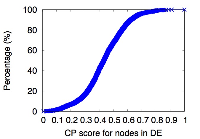
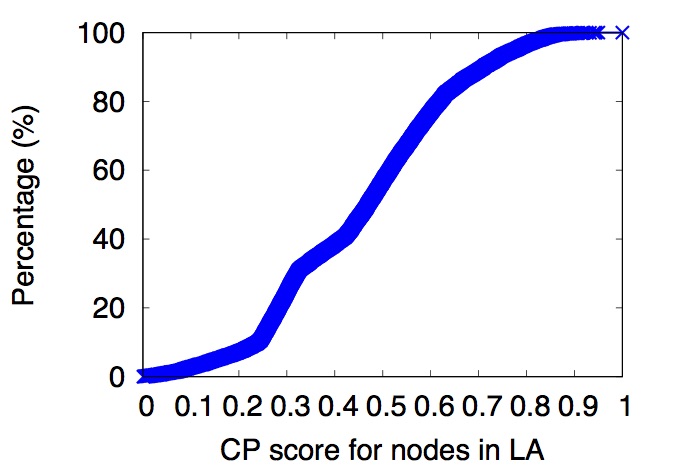
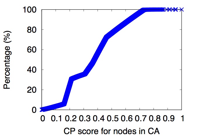
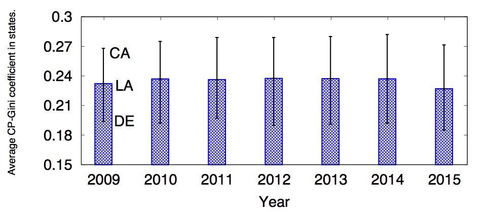
Figure 2: Counterclockwise from upper right: CP score distribution of LA, DE, and CA (minimu, median, maximum), in 2009 and the distribution of Gini coefficients of CP score among the 50 states over 2009-2015.

The uneven distribution of CP scores suggests a strong Core-Periphery structure in these state networks. Strong Core-Periphery structure is a trait seen generally across all of the state-level networks. The Gini coefficient of CP scores for all nodes in a state is increasing from 2009 to 2014 suggesting that physician involvement in patient care is forming a stronger core-periphery as time passes.

3.2 Degree-, clustering-, and connectivity-related statistics

Degree Distributions and Power Laws. We computed the in- and outdegree distributions for both the national network and the fifty intrastate networks. The nearly zero p-value of the goodness of fit test against the null hypothesis rejects that the degree distribution is Poisson. Furthermore, the clear difference in terms of clustering coefficient in Table 2 contributes to a rejection of the Erdós-Renyi random graph model for the data.

We next check for a power law. The intuition for considering a power law comes from one of the generative models witnessed in many networks (cf., [27, 30]): the so-called “rich get richer” process. This is perhaps the best known power law-producing generative process, wherein nodes acquire new connections at random but in proportion to their current number of connections. It is plausible that there are groups of physicians (e.g., certain types of specialists) that receive and possibly make many more referrals than others and furthermore that physicians accrue new ties in proportion to their existing number of ties. Reputation spread may also manifest as a power law. In contrast, if physicians with many referrals are less likely to accept new referrals (e.g., they stop taking new patients) and are content with their existing set of “partner physicians” for referrals, the degree distribution would be expected to be more uniform than depicted by a power law.

In a log-log plot, a power law will appear as a (roughly) straight line. The lefthand of Figure 3 shows the power law fitting figure for the 2015 Delaware Intrastate Referral Network. The straight line of the log of Delaware’s (unweighted) degree distribution matches the form implied under a power law. The righthand side shows the distribution of the p-value statistic for testing the null hypothesis that the distribution in the network is a power law in the outdegree using the national 2012 data as an example. We also test the power law hypothesis for both indegree and outdegree among all 50 intrastate networks as well as the whole national network. For the majority of states (approximately 80%), the p-values of both the indegree and outdegree distributions are greater than $0.05$, so we fail to reject the null hypothesis that the degree distribution is generated from a power law. Table 2 summarizes the p-value statistics across several years, and Figure 4 shows the state map of average p-values in 2009-2015. If there was a power law in every state then the p-values for the power law test would follow a uniform distribution. Therefore, to make a claim of whether the power law is universal across all states, we test whether the empirical distribution of the p-values is uniform using the Shapiro-Walks (or a K-S) test. Because the null hypothesis of a uniform distribution is rejected, we conclude that there is strong evidence that the power law is not universal.

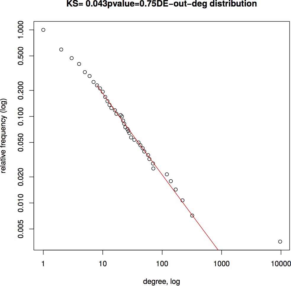
Figure 3: Out-degree of DE in 2015. P-value distribution of degree-out in 2012 for all states.

Figure 4: State map of average p-values of Power Law Test in 2009-2015, for both indegree and outdegree.

The data in Table 2 suggest that the outdegree distributions seem to have a stronger tendency toward power law than indegree. Herein we find the number of states with a p-value $\geq 0.05$. Because a physician does not control who refers patients to them, the number of distinct physicians sending patients may exceed the proportional growth. This is supported by the observation that the indegree distribution has a greater spread than outdegree. Alternatively, the departure of the indegree distribution from a power law might be due to certain specialist physicians being absorbing nodes in the sense that they are the last step in the patient’s care (e.g., a sub-specialist).

The indegree and outdegree distributions of the national and intrastate networks show power laws with large p-values in Table 2 only except outdegree in 2013. Figure 5 shows the log-log plot of the three national networks, including the indegree and outdegree log-log plot in 2009 with p-value=$1.0$ and the corner case of outdegree in 2013. The three groups of degree distribution have similar patterns, although the p-values vary.

Figure 5: Degree Power Law of national network.

Assortativity. Table 2 displays the average correlation coefficient between two degree values on edges of the 50 state induced referral networks. Given the directed nature of the networks, three kinds of degree assortativity can be measured. We find (in-,in-) and (out-,out-) degree correlations exhibit mildly negative assortativity, which means patient referral has a small tendency to occur between physicians who possess different levels of indegree or different levels of outdegree. The significance of the assortativity values against a null hypothesis of no assortativity is tested under an ER null network by using the fact that the asymptotic standard error of $0.5\log((1-r)/(1+r))$ is $SE=(n-3)^{-1/2}=3.35-9.78*10^{-4}$, where $r$ denotes the given Pearson correlation coefficient of the respective degree frequencies and $n$ is the number of physicians in the network. Because the assortativity values are far from 0, it is clear that assortativity is significantly different from 0 in all cases.

Correlation of in-degree and out-degree. Table 2 shows the measurement of correlations between indegree and outdegree on the same physician in several years. Since the correlation coefficients in all states are very close to $1.0$, only average values are reported. The results imply that physicians who receive a lot of referrals also make a lot of referrals. The correlation may be inflated due to the fact that specialty is not controlled for and past research [3] has shown that degree varies substantially between specialties; if the correlation was measured within physician-type the correlation would likely be lower.

Reciprocity. If we consider the weight on edges in a directed network, Table 2 shows the R-squared value and correlation coefficient of $w_{ij}$ and $w_{ji}$. The bidirectional weights have strong correlations in different years. Reciprocity reflects the professional relationship between physicians. The observations support the idea that physicians refer patients back to the referring physician once the specialty appointment is complete or distinct patients see the physician dyad members in opposite orders. Either way, high reciprocity reflects stable collaboration.

Clustering coefficient. Figure 6 illustrates both global and local clustering coefficients of states in several years. The error bars show the range of the coefficient values with error bars.

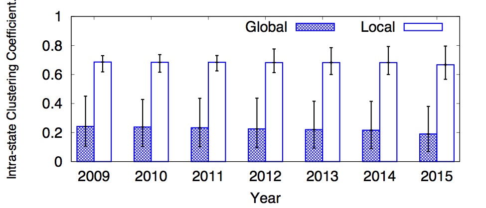
Figure 6: Clustering coefficients of state network in 2009-2015

Table 2 shows the clustering coefficient in the whole national referral network. The local clustering coefficient is much larger than the global one, reflecting a positive correlation between geographic closeness and network flow. The expected local clustering coefficient in an Erdos-Renyi model [13] $p=\mu/(n-1)$ is much smaller than the measured results. Taken together with the above discussion, we conclude that the patient referral networks have small world character.

Core Physician Connectivity Patterns. Each state will have one and only one node with the CP score of $1.0$. We extract those core nodes from each state in 2009-2015 and consider the network constructed by counting the number of cross-state referrals between a core node and external states in Figure 7. The core nodes in FL and ML have the widest connectivity, each connecting with physicians in more than 30 other states. On the other hand, the core node in HI only refers or receives patients from 4 external states (presumably a reflection of the distance of Hawaii from the mainland). The core nodes in DE, MS and FL include the most interstate referrals in 2009-2015. The fact that FL has so many referrals is a reflection of the “snowbird phenomena” whereby a large number of residents of northern states move to southern states, the most popular of which is Florida, for the winter. The same may be partially true of Mississippi.

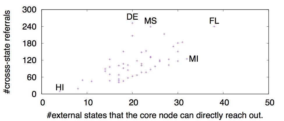
Figure 7: Number of states that a core node with CP score $1.0$ connects to, and the number of cross-state referrals for the corresponding core node. Time ranges from 2009-2015.

Figure 8: The state map of Figure 7 and core node connections.

A Skeletal National Network and Gravity Law. Figure 9 displays for each state the connections to the top five states to which its physicians make referrals. NY, PA, FL, TX, CA, MI, MA play the role of “hub” states, while midwestern states do not have many cross-state referrals. In general, the traffic map matches the population distribution in the U.S.

The flow of patients around the country – as represented by referral data – suggests that the tools and models of economic geography might be relevant. Most famous is the well-known “gravity law” of the type defined by Equation 2:

$$F_{ij}=G\frac{M_{i}^{\beta_{i}}M_{j}^{\beta_{j}}}{D_{ij}^{\beta_{d}}},$$ (2)

where $F_{ij}$ represents the number of distinct patients referred from state $i$ to state $j$, $G$ is a constant, $M_{i}$ and $M_{j}$ represent the number of physicians in states $i$ and $j$, respectively, and $D_{ij}$ denotes the distance between the two capital cities. Such a “law” is commonly fit to macroeconomic trade patterns. [19] Based on referral records in 2009-2014, an OLS method is used to estimate the $\beta$ coefficients. $\hat{\beta}_{i}=0.904,\hat{\beta}_{j}=0.904,\hat{\beta}_{d}=1.342$ so that the number of distinct patients is inversely proportional to the distance, which validates the hypothesis of a gravity law. As further support, in a log-log plot the linear relationship between $F_{ij}$ and $M_{i},M_{j},D_{ij}$ is significant with p-value $<2.2e-16$, residual standard error 2.258, R-squared 0.5764.

Figure 9: A visualization of the top five out-of-state referrals. Edge width varies by percentage of within-state referrals, and node size varies by size of state’s physician referral network. The map depicts directed edges of each state’s top five states to which they refer patients. Note that nodes for Alaska (AK) and Hawaii (HI) are placed in the bottom left of the figure. As this is a network diagram, the placement position is not relevant.

3.3 Motif analysis

Network “motifs” are commonly recurring small patterns of connectivity, often thought of as a network’s “building blocks”. [26] Dyadic motifs are the simplest in structure having just two nodes and in a directed binary-valued network only a few possible states. If the motifs do not distinguish between the edge from physician A to B and that from B to A, there are only three dyadic paterns: no edge, one directional edge and bidirectional edges. While no-edge case is dominant in terms of frequency, the fraction of Monte-Carlo estimated frequency of directional dyads and bidirectional dyads is around 24:76, implying a very high-level of reciprocity is present in the network. As a part of the exploration of patterns in patient referral networks we engaged in exploratory analysis to discover what kinds of triads in our directed networks are most prevalent. Figure 10 illustrates the 16 possible triads.

Figure 10: 16 kinds of triads

Table 3 displays the Monte-Carlo estimated frequency of the various triad structures (i.e., randomly sample node 3-tuples and record the connectivity structure) over 2009-2015 in the national network (a Monte Carlo calculation of $10^{8}$ random draws was used because complete enumeration is infeasible). The completely disconnected triad (Triad 1 in Figure 10) is far and away the most prevalent and we do not record its number. The remaining 15 kinds of triads break up naturally in terms of order of magnitude of frequency into 7 groups: (1) Triads 2 and 3: Two physicians share patients in one or two directions; (2) Triad 11: a physician shares patients with two physicians mutually; (3) Triads 7 and 8: a physician shares patients with one physician mutually and with another physician in only one direction; (4) Triads 5,6,15, and 16: loose connections and close connections between three physicians; (5) Triads 12, 13, 14: a pair of mutually connected physicians with the third physician whose degree is two; (6) Triad 9: a triple that follows transitivity (if A refers a patient to B and B refers a patient to C the chance that A referred a patient to C is substantially greater than otherwise) and lastly (7) Triad 10 without transitivity.

Since the referral records do not contain patient ID, we cannot track the same patient and analyze the referral sequence. The rank order remains roughly the same over each year suggesting that the structure of the network is stable in this regard. Triad 2 and Triad 3 are the two most popular triad patterns in the whole referral network, accounting for the majority of the triads in the state networks. These convey two of the most elementary care patterns. Under Triad 2, a patient encounters physician A followed by physician B and then is done. Under Triad 3 the patient emulates the care pattern of Triad 2 but then returns to see physician A again. The frequency distribution suggests that the network contains regions of high density, or even cliques, since some triads with more edges (T15 and T16), representing more complex care patterns within reciprocated referrals between 2 or 3 physicians, occur more frequently than triads with fewer edges (T9, T10, T12, T13, T14).

To detect the latent groups of triads, we remove the columns of the correlation matrix corresponding to Triads 2 and 3, which remain as their own groups, and perform a factor analysis on the correlation matrix for Triad types 4-16. Table 4 displays the factor loadings on those triads for 2009-2015. Assuming two factors, the groups of triads based on highest loading correlation are (T4, T9, T10, T12, T13, T14, T15, T16) and (T5, T6, T7, T8, T11). With three latent factors, the loadings also support this group division as for the two-factor case.

The factor analysis provides more flexibility for the regression analyses performed in Section 4. For these analyses we have limited observations, 50 states observed in 5 years for a total of 2,500 observations. The clustering of observations within states reduces the information content of the data. Our ideal model would simultaneously estimate the effect of all network-based predictors, and any other predictors, on each of these dependent variables. With a modest number of observations, the model is vulnerable to over-specification if an excessive number of predictors are included. As opposed to including 15 measures of the relative frequency of each type of triad, we instead may include the relative frequency measures for two of the three groups of triads allowing more flexibility in regards to including other predictors, interaction variables, and transformed predictors. In building the hierarchical model in Section 4, we test whether replacing the individual triad predictors with their factor-based groups was justified by comparing the total variation explained by all of the triad indicators to that explained by the grouped variables and testing the significance of the difference. To ensure that the grouped triadic variables captured triadic or higher-level effects and not dyad-level effects, the level of reciprocity in each state and year was also included as a predictor in any model containing triad-level predictors.

3.4 Diversity among states

From hereon, we discard the data in 2015 since the period of observation is not complete and many healthcare attributes are not available in 2015.

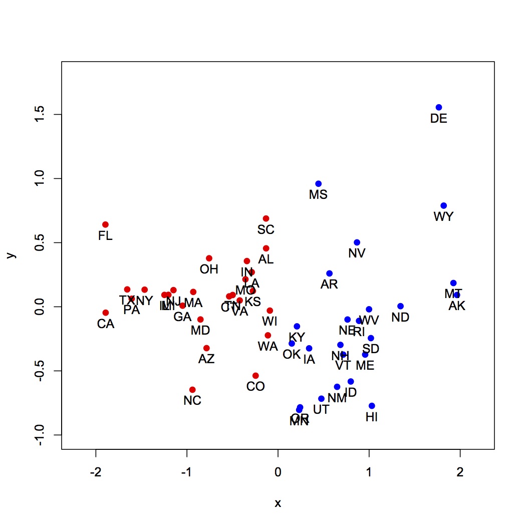
Figure 11: Multidimensional scaling (MDS) plot of 50 states based on feature vector in 2014. Two clusters are in red and blue.

We apply the K-means clustering algorithm to the 50 feature vectors defined by the state-level network measures in Table 9. Figure 11 is a 2-d visualization, produced via multidimensional scaling (MDS). The red and blue coloring of the nodes represents the outcome of applying K-means with two clusters, for which the centroids are MA (red) and ME (blue) respectively. We find that the cluster represented by MA generally includes the states which have more physicians or larger population than those of the cluster represented by MA. Table 5 shows the centroid states of each cluster for $K=2,3,4,5$.

4 Comparative Analysis: Relationships Between Network and Healthcare Measures

Table 6 shows selected univariate correlations (i.e., not accounting for the possible overlapping effects of any other predictors) between network measurements and healthcare statistics in 2009-2014 for all state-years. The presence of such high correlations suggest the potential for estimating a multiple regression model that exhibits a high level of predictive accuracy. Because the data contain repeated measurements on states, our core statistical regression model is a mixed-effect model with state random effects. Denoting an outcome and vector of network measures for state $i=1,\ldots,50$ in year $t=0,\ldots,5$ by $Y_{it}$ and $X_{it}$, respectively, the mathematical specification of these models has the following general form:

$$Y_{it}=\alpha_{i}+\lambda_{t}+\bm{\beta}_{1}^{T}\bm{X}_{it}+\bm{\beta}_{2}^{T}\bm{X}_{it}t+\varepsilon_{it}$$ (3)

where $\alpha_{i}\sim N(\beta_{0},\tau^{2})$ describes the distribution of the state-level random effects and $\varepsilon_{it}\sim N(0,\sigma_{y}^{2})$ describes the distribution of the error term. The main effect of the vector of network measures is $\beta_{1}$ while its modification by linear year ($t$) is $\beta_{2}$. The parameters $\lambda_{t}$ allow for an unstructured population trend across years whereas the state-specific departures from this trend are restricted to be linear (i.e., proportional to $t$). Modeling the time-trend as an unstructured (maximally flexible) main effect and linearly as a network effect modifier serves the purpose of fully capturing the population trend (the variation we want to control for) and parsimoniously representing the effect-modification by time (the effect of interest that we want to interpret). It also allowed for more stable estimation than when seeking to estimate separate effects of the network measures in each year.

Separate models of the form given in Equation 3 were estimated for each of the 20 state-level health attributes. Therefore, the initial model for each dependent variable allowed the coefficient of the network predictors to change linearly with time. If the interaction of linear time with a given network measure is non-significant, it was dropped from the final specification. To determine the model for each health care outcome, we used a model building process that sought to obtain a parsimonious set of models with a common set of predictor variables across the outcomes. Starting with the predictor with the strongest univariate effect, we added predictors one at a time until no more predictors that had significant effects could be added. We repeated the same process across all outcomes. The final set of network measures was obtained by taking the union of all included network measures across the outcomes; we denote the size of this set by $M$. For each outcome, we then added all of the interactions of these predictors with $t$ and starting with the least significant dropped them one-by-one until only significant terms remained. For both the inclusion and exclusion steps, we use a chi-squared test of the magnitude of variation in the outcome across the levels of the predictor to determine if the predictor accounts for a significant amount of variation, justifying its inclusion in the model, or if it adds minimal or no explanatory power and can be excluded. The final models thus contained the same network measures but differed in terms of how of them many had significant linear interactions with time. For example, when medical-discharge-per-1000-people (called f34) is the dependent variable, none of the selected network features had a significant linear interaction with time, so the interaction predictor is absent.

As Table 8 reveals, the selected features for the regression of medical-discharge-per-1000-people (f34) are: average-degree (f1), (out-, out-) assortativity in induced-network (f25) and the Gini coefficient of sizes of the components (groups of nodes with no edges between them) of the induced network (f16). Table 7 shows the change of coefficients for selected predictors from model 1 to model 3 in Table 8. The coefficients range from 4.08 to 14.70 and are directly comparable as the predictors were standardized to a mean of 0 and standard deviation of 1. According to m3, the dependent variable (f34) is more sensitive to f1, and changes in the referral network are associated with healthcare attributes.

4.1 Result analysis

Some features (e.g., f1, f5, f9, marked with asterisk) have significant interactions with time (each year) for several healthcare attributes in Table 8, because they are related to the increasing size of the referral network (Table 1). The coefficients of interaction items are in Table 10. None of the triadic predictors warranted inclusion in the final model for each outcome.

Across individual healthcare measures the most prominent network-based predictors involve the physician degree (the density of the network – f1), number of physicians in the intra-state network (f9), out-degree (out-,out-) assortativity of the induced network, and heterogeneity of the size of the networks components as computed by the Gini coefficient (f16). The general assortativity results imply selectiveness of physicians to seek out physicians like themselves (i.e., those with similar patient referral tendencies) when making patient referrals while the component size distribution reflects co-existence of large provider groups and independent practices in a region. It is unclear whether these are characteristics of a region that could be exploited to incite more efficiency or otherwise improve healthcare. For further illustration, we consider significant network predictor-outcome pairs and provide illustrative interpretations with respect to particular outcomes, recognizing that these points only suggest a direction of possible investigation, but lack obvious explanations.

• For medical-discharge-per-1000-people the high associations are average degree (f1), assortativity (f25) and Gini coefficient of component size (f16). The positive coefficients might reflect that more discharges from hospital might lead to or generate more follow-up care.

• Hospital-admissions-per-1000-decedents is understandably highly correlated with the number of patient referrals. This might be a front-end of the above result – both hospitalizations and discharges from hospital may be a result of or generate more referrals.

• For long-term-opioids-receipt (see [25] for description), the clustering coefficient (f7 and f20) has a significant negative effect suggesting that networks with greater closure better contain overall opioid consumption (e.g., through better patient monitoring).

• Gross State Product (GSP) is associated with the Gini coefficient of in-degree; one possible explanation is that having a few physicians who receive an extreme number of referrals might be a marker of a state having the capability to perform rare, highly complex procedures.

• For the regression of #nodes-per-1000-people both average degree and global clustering coefficient have large estimated coefficients. A larger average degree implies that more physicians are working in the state, possibly indicating a form of supply driven utilization. [33]

• A uniform distribution of physicians and a low clustering coefficient are associated with more physicians being shared per 1,000 people. This may indicate that patients do more physician shopping (searching for physicians who’ll approve the pharmaceuticals or procedure they seek) in states whose physician networks have less closure (i.e., less clustering).

• Mortality is associated with average degree and #edges. This is an interesting finding but before making conclusive interpretations it would be important to control for patient demographic and clinical variables.

• Gini coefficient of out-degree (f5) has a large association with expense-per-inpatient-day suggesting that patients on average pay more for treatment in states with greater heterogeneity of physician popularity. Again, this may be a marker for the availability of specialty services in the state.

• For the regression of #hospital-beds-per-1000-people the Gini coefficient measures (f5 – out-degree distribution and f16 – component size) both have negative estimated coefficients suggesting that the more that care is regionalized at select institutions (perhaps by those performing the majority of a given specialty or performing some kind of other non-standard care), the less the need for hospital beds.

5 Conclusion

In this paper, we applied algorithms and methods from graph theory, network science and statistics to explore many network features in the U.S. patient referral networks. Those network features describe both micro and macro patterns about patient referrals, such as power laws in some degree distributions, “small world” structure, Core-Periphery structure, motifs of triadic structures, and “Gravity Law” in cross-state referrals. Indeed, with the last of these we suggest implicit broader connections with economic geography (see e.g., [19]) which are intriguing and suggest natural follow-ons. We also find close correlations between network features and state healthcare attributes. A better understanding of network features may provide insights into directions for improving the healthcare system. Our findings come with the caveat implicit that the data only includes referrals within the Medicare system. Nevertheless, the fact that we use only data that is available to the public means that our methods and results can be replicated. This furthermore supports one of our key goals of introducing the growing network science toolkit (measures, tools, and models) to statisticians and medical researchers who are less familiar with generative models in particularly as well as empirical models for social network data, and to also show that these ideas can be deployed on a very large scale.

From 2009-2015 we found that the majority of network features are fairly stable. Our key results encompass both general or macro-level and micro-level network features. At the macro-level, the power law structure cannot be rejected in most cases, which suggests that these networks are “robust yet fragile” – i.e., robust to random failure, but susceptible to “targeted” attack (i.e., consciously specified removal). [1] The small-world property implies that physician networks are suitable for efficient information transfer and diffusion of innovations. [43] Analyses at both state and national network level tends to support the hypothesis of a “small world” and thus a fertile environment for diffusion (see also [38] and [18] for other possible connections) and suggests a rich direction of future research. At a micro-level, the computation of actor specific network measures allows rankings of physicians to be constructed based on their importance in the referral network. Possible measures that can be used include degree, local clustering coefficient, CP score, and the number of external connections.

By evaluating associations between the network measures for each state and health variable, we gain insights into how improvements in health care organization and ultimately outcomes might be incentivized. For example, we found that clustering was positively associated with per-capita state opioid prescription fills. Therefore, to reduce over-use of opioids, a public health intervention that sought to limit referrals among the highest prescribing physicians could be investigated.

In general, to optimize the referral network in terms of healthcare system efficiency and physician workload, we hope that lessons can be learned from understanding the network aspects of the most well-performing states and consequent investigation of whether it might be useful to try to extend or even enforce such structures in other states. A natural next study that still only uses freely available data would be to incorporate physician specialty (unlike patient data, information on physicians is publicly accessible) in order to both distinguish physician network effects from physician specialty effects and also to reveal specialty-network interaction effects. However, the ultimate goal is to link the national physician network to individual patient data in order to perform patient-level analyses that account for patient demographic and clinical factors when assessing the association of the physician network and its salient subnetworks to important patient outcomes.

Table 1: Dataset size by year.

Year	2009	2010	2011	2012	2013	2014	2015
#Records	50,382,951	52,236,906	54,038,549	54,966,715	55,141,669	55,779,360	34,856,901
#Physicians	890,452	921,959	955,659	987,770	1,018,245	1,044,758	961,309

Table 2: P-values for rejecting various Power Laws, assortativity, self-degree-correlation, reciprocity and clustering coefficient of the national patient referral network (or average among states) in 2009-2015.

Year	2009	2010	2011	2012	2013	2014	2015
in-degree p-value of national network Power Law	1.00	0.99	1.00	1.00	0.93	0.91	0.38
#states in-degree p-value>0.05	32	37	37	36	36	37	36
Average p-value of in-degree Power Law among states	0.4084	0.4084	0.4137	0.4245	0.4423	0.4388	0.4654
out-degree p-value of national network Power Law	1.00	1.00	0.99	0.97	0.00	0.97	0.74
#states out-degree p-value>0.05	39	43	42	37	37	38	40
Average p-value of out-degree Power Law among states	0.4545	0.5292	0.5913	0.5303	0.5190	0.4956	0.4484
Average (in, in) assortativity among states	-0.1084	-0.1083	-0.1101	-0.1126	-0.1132	-0.1137	-0.1217
Average (out, out) assortativity among states	-0.1104	-0.1108	-0.1125	-0.1150	-0.1157	-0.1161	-0.1245
Average (in, out) assortativity among states	0.0775	0.0752	0.0727	0.0692	0.0662	0.0633	0.0549
Average (out, in) assortativity among states	0.0800	0.0775	0.0750	0.0714	0.0684	0.0654	0.0569
State self in/out degree: average R-squared value	0.9717	0.9715	0.9712	0.9717	0.9710	0.9711	0.9692
State self in/out degree: average correlation coefficient	0.9858	0.9856	0.9855	0.9857	0.9853	0.9854	0.9845
State reciprocity: average R-squared value	0.9074	0.9094	0.9073	0.9053	0.9045	0.9015	0.8927
State reciprocity: average correlation coefficient	0.9524	0.9535	0.9524	0.9513	0.9509	0.9493	0.9445
global clustering coefficient of national network	0.0763	0.0740	0.0727	0.0682	0.0623	0.0609	0.0523
local clustering coefficient of national network	0.700	0.699	0.698	0.698	0.698	0.699	0.691
E(C) by Erdós-Renyi Model of national network	1.27e-4	1.23e-4	1.18e-4	1.13e-4	1.06e-4	1.02e-4	7.54e-5

Table 3: Triad frequencies for the U.S. national referral network.

ID	2	3	4	5	6	7	8	9	10	11	12	13	14	15	16
2009	23433902	76245745	188	4096	5113	56061	28650	66	1	222166	171	127	157	1484	2073
2010	23747795	75929710	206	4426	5321	58748	28634	49	4	221342	176	117	141	1427	1904
2011	23865204	75802642	175	4999	5720	62887	29448	56	0	225125	166	124	144	1342	1968
2012	23892310	75764994	167	4989	5811	64475	30656	63	1	233164	163	99	127	1264	1717
2013	24202517	75439104	180	5648	6524	68943	31777	51	5	242030	155	114	125	1185	1642
2014	24405405	75233266	201	5803	6571	69167	32792	51	4	243538	174	104	109	1210	1605
2015	25421893	74265148	147	5160	6326	59787	31480	52	2	207622	140	90	86	948	1119

Table 4: Factor analysis loadings of state level triad terms over 2009-2015.

#Factors=2	T4	T5	T6	T7	T8	T9	T10	T11	T12	T13	T14	T15	T16
Factor1	0.853	0.608	0.536	0.348	0.346	0.872	0.909	0.182	0.896	0.912	0.923	0.926	0.938
Factor2	0.513	0.756	0.836	0.880	0.868	0.453	0.399	0.687	0.408	0.397	0.397	0.357	0.278
#Factors=3	T4	T5	T6	T7	T8	T9	T10	T11	T12	T13	T14	T15	T16
Factor1	0.870	0.644	0.574	0.370	0.372	0.894	0.920	0.175	0.920	0.929	0.939	0.937	0.944
Factor2	0.466	0.654	0.753	0.897	0.876	0.358	0.367	0.815	0.309	0.342	0.326	0.346	0.297
Factor3	0.123	0.329	0.279	0.110	0	0.249	0	-0.116	0.224	0.109	0	0	-0.129

Table 5: The nearest states to the centroids of the clusters of states obtaining using K-means.

Year\#cluster	n=2	n=3	n=4	n=5
2009	ME MA	LA NC SD	NC OR SD TX	KY MA OR SD TX
2010	ME NC	LA PA SD	LA OR PA SD	LA ME OR PA SD
2011	ME MD	IL PA SD	LA NM PA SD	LA MT NM PA SD
2012	ME MA	ME PA TN	ME PA SD TN	LA ME MT PA TN
2013	ME MA	ME MI TN	MI MT OR TN	MI MT NE OR TN
2014	ME MA	ME MI MT	ME MI MT TN	ME MI MT NE TN

Table 6: Selected correlations between network measures and state healthcare measures.

Network	Healthcare	R-square	Correlation coefficient
#edges	#population	0.813	0.902
average degree	medical reimbursement	0.662	0.814
Gini coefficient of CP score	#physicians	0.578	0.760
assortativity (in, in)	#medicare beneficiaries	0.491	0.701
assortativity (in, out)	state expenditure per person	0.317	0.563
average degree	average contact days	0.500	0.706
Gini coefficient of CP score	average contact days	0.339	0.582
average degree	inpatient days in hospital	0.565	0.751
Gini-outdeg	expense-per-inpatient-day	0.429	0.655
global cluster coefficient	#physicians	0.358	-0.598

Table 7: Stability of estimated effects of network predictors for four network features: average-degree (f1), (out-, out-)-assortativity in induced-network (f25) and Gini coefficient of component size distribution in induced network (f16). The changes in one predictor when others are added reflects the collinearity between the predictors.

Model	Selected Network Features	Coefficient ($\beta_{1}$)
m1	f1	19.11
m2	(f1, f25)	(16.03, 8,56)
m3	(f1, f25, f16)	(14.70, 6.92, 4.08)

Table 8: Associations between healthcare attributes and network features. f1 (average degree). A full list of potential predictors/network features is in Table 9. The features with an asterisk also have significant interactions with time for the corresponding healthcare attribute. The coefficients of interaction items are in Table 10.

Healthcare Attribute	Selected Network Features	Corresponding Coefficients
medical-discharge-per1000-people	(f1, f25, f16)	(14.70, 6.92, 4.08)
hospital-admissions-per1000-decedents	(f1, f22, f25, f$16^{*}$)	(84.04, 16.58, 15.22, 17.99)
long-term-opioids-receipt	(f1, f7, f20, f26, f24)	(0.70, -0.077, -0.32, 1.30, 0.82)
general-inpatient-days-in-hospital	(f$1^{*}$, f25, f18)	(0.14, 0.050, 0.0051)
medical reimbursement per capita	(f23, f$29^{*}$, f30)	(-1.6e-5, 4.1e-5, -1.4e-3)
Gross State Product (GSP)	(f$9^{*}$, f22, f$17^{*}$, f1, f3)	(459892.4, -79067.3, -21304.8, -8886.8, -10331.9)
#medicare-beneficiaries	(f$9^{*}$, f5)	(974692.9, -59712.4)
#nodes-per-1000-people	(f$1^{*}$, f6, f19)	(0.16, 0.023, -0.15)
mortality	(f1, f16, f10)	(0.12, -0.038, -0.12)
expense-per-inpatient-day	(f$5^{*}$, f7, f9)	(125.63, -85.44, 55.05)
#hospital-beds-per-1000-people	(f7, f$1^{*}$, f$5^{*}$, f16, f$26^{*}$, f29)	(0.048, 0.44, -0.13, -0.11, 0.39, -0.012)

Table 9: Full list of network features for the mixed-effect (hierarchical or multi-level) regression model.

Feature ID	Name
f1	average degree of intra-state network
f2	$\alpha$ of in-degree Power Law of intra-state network
f3	Gini coefficient of in-degree distribution of intra-state network
f4	$\alpha$ of out-degree Power Law of intra-state network
f5	Gini coefficient of out-degree distribution of intra-state network
f6	diameter of intra-state network
f7	global clustering coefficient of intra-state network
f8	local clustering coefficient of intra-state network
f9	#nodes in intra-state network
f10	#edges in intra-state network
f11	undirected assortativity of intra-state network
f12	(in-,in-)assortativity of intra-state network
f13	(out-,out-) assortativity of intra-state network
f14	(in-,out-)assortativity of intra-state network
f15	(out-,in-)assortativity of intra-state network
f16	Gini coefficient of component size distribution of induced network
f17	size of dominant component of induced network
f18	diameter of induced network
f19	global clustering coefficient of induced network
f20	local clustering coefficient of induced network
f21	#nodes in induced network
f22	#edges of induced network
f23	undirected assortativity of induced network
f24	(in-,in-)assortativity of induced network
f25	(out-,out-) assortativity of induced network
f26	(in-,out-)assortativity of induced network
f27	(out-,in-)assortativity of induced network
f28	Gini coefficient of CP scores for all nodes in a state
f29	entropy of the core node distribution under different parameter settings
f30	#states that the core node in terms of CP score can directely reach out
f31	#cross-state referrals of the core node in terms 1.0 CP score in 2009-2014

Table 10: Coefficients of significant interaction terms with linear time (in units of years) in the mixed-effect regression model.

Healthcare Attribute	Network Feature	Time (year)	Coefficients of Interaction Items ($\beta_{2}$)
hospital-admissions-per1000-decedents	f16	2010-2012	(5.35, 9.54, 0.52)
general-inpatient-days-in-hospital	f1	2010-2012	(-0.0072,-0.019,-0.040)
medical reimbursement per capita	f29	2010-2012	(-2.2e-05, 8.7e-06, -4.9-05)
Gross State Product (GSP)	f9	2010-2012	(29883.2, 55874.3, 88033.6)
Gross State Product (GSP)	f17	2010-2012	(-24454.9, -44870.2, -64875.2)
#medicare-beneficiaries	f9	2010-2012	(10274.3, 20157.3, 35119.1)
#nodes-per-1000-people	f1	2010-2014	(0.030, 0.042,0.065,0.090,0.098)
expense-per-inpatient-day	f5	2010-2014	(4.0, 22.5, 41.1, 46.7, 64.5)
#hospital-beds-per-1000-people	f1	2010-2014	(-0.22, -0.19, -0.19, -0.15, -0.17)
#hospital-beds-per-1000-people	f5	2010-2014	(-0.12, -0.11, -0.10, -0.10, -0.10)
#hospital-beds-per-1000-people	f26	2010-2014	(-0.30, -0.27, -0.30, -0.30, -0.32)

References

- [1] R. Albert, H. Jeong, and A. Barabasi. Error and attack tolerance of complex networks. Nature, 406:378–382, 2000.
- [2] M. Barnett. Mapping physician networks and their association with health care delivery in us hospitals. MD Thesis, Harvard Medical School, Boston, MA, 2011.
- [3] M. Barnett, N. Christakis, A. O’Malley, J. Onnela, N. Keating, and B. Landon. Physician patient-sharing networks and the cost and intensity of care in us hospitals. Medical care, 50(2):152, 2012.
- [4] M. Barnett, N. Keating, N. Christakis, A. O’Malley, and B. Landon. Reasons for choice of referral physician among primary care and specialist physicians. Journal of General Internal Medicine, 27(5):506–512, 2012.
- [5] M. Barnett, B. Landon, A. O’Malley, N. Keating, and N. Christakis. Mapping physician networks with self-reported and administrative data. Health Services Research, 46(5):1592–1609, 2011.
- [6] M. Barnett, Z. Song, and B. Landon. Trends in physician referrals in the united states, 1999-2009. Archives of Internal Medicine, 172(2):163–170, 2012.
- [7] A. Chukmaitov, K. Devers, D. Harless, N. Menachemi, and R. Brooks. Strategy, structure, and patient quality outcomes in ambulatory surgery centers (1997-2004). Medical Care Research and Review, 68(2):202–225, 2011.
- [8] A. Clauset, C. Shalizi, and N. ME. Power-law distributions in empirical data. SIAM Review, 51(4):661–703, 2009.
- [9] CMS. Physician shared patient datasets. https://questions.cms.gov/faq.php?faqId=7977. Accessed Sept 1, 2016.
- [10] CMS. Physician shared patient patterns methodology. Technical report. https://downloads.cms.gov/foia/physician_shared_patient_patterns_technical_requirements.pdf. Accessed Sept 1, 2016.
- [11] M. Cowan, M. Shapiro, R. Hays, A. Afifi, S. Vazirani, C. Ward, and S. Ettner. The effect of a multidisciplinary hospitalist physician and advanced practice nurse collaboration on hospital costs. Journal of Nursing Administration, 36(2):79–85, 2006.
- [12] CRAN. Power law r-package. Technical report. https://cran.r-project.org/web/packages/poweRlaw/index.html. Accessed Oct 1, 2016.
- [13] P. Erdós and A. Renyi. On random graphs, i. Publ. Math, 6:290–297, 1959.
- [14] C. Forrest, P. Nutting, B. Starfield, and S. Von Schrader. Family physicians’ referral decisions: results from the aspn referral study. Journal of Family Practice, 51(3):215–223, 2002.
- [15] M. Granovetter. The strength of weak ties. American Journal of Sociology, 78(6):1360–1380, 1973.
- [16] T. Iwashyna, J. Christie, J. Kahn, and D. Asch. Uncharted paths: hospital networks in critical care. CHEST, 135(3):827–833, 2009.
- [17] W. Knaus, E. Draper, D. Wagner, and J. Zimmerman. An evaluation of outcome from intensive care in major medical centers. Annals of Internal Medicine, 104(3):410–418, 1986.
- [18] G. Kossinets, J. Kleinberg, and D. Watts. The structure of information pathways in a social communication network. 14th ACM SIGKDD conference. pp. 435-443, 2008.
- [19] P. Krugman. Development, Geography, and Economic Theory. MIT Press, Cambridge, MA, 1997. Vol.6.
- [20] B. Landon, N. Keating, M. Barnett, J. Onnela, S. Paul, A. O’Malley, T. Keegan, and N. Christakis. Variation in patient-sharing networks of physicians across the united states. JAMA, 308(3):265–273, 2012.
- [21] B. Lee, S. McGlone, Y. Song, T. Avery, S. Eubank, C. Chang, R. Bailey, D. Wagener, D. Burke, R. Platt, and S. Huang. Social network analysis of patient sharing among hospitals in orange county, california. American Journal of Public Health, 101(4):707–713, 2011.
- [22] B. Lee, Y. Song, S. Bartsch, D. Kim, A. Singh, T. Avery, S. Brown, S. Yilmaz, K. Wong, M. Potter, and D. Burke. Long-term care facilities: Important participants of the acute care facility social network? PLoS ONE, 6(12):e29342, 2011.
- [23] A. Lomi, D. Mascia, D. Vu, F. Pallotti, G. Conaldi, and T. Iwashyna. Quality of care and interhospital collaboration: A study of patient transfers in italy. Medical Care, 52(5):407–414, 2014.
- [24] K. Mandl, K. Olson, D. Mines, C. Liu, and F. Tian. Provider collaboration: cohesion, constellations, and shared patients. Journal of General Internal Medicine, 29(11):1499–1505, 2014.
- [25] E. Meara, J. Horwitz, W. Powell, L. McClelland, W. Zhou, A. O’Malley, and N. Morden. State legal restrictions and prescription opioid use among disabled adults. New England Journal of Medicine, 375:44–53, 2016.
- [26] R. Milo, S. Shen-Orr, S. Itzkovitz, N. Kashtan, D. Chklovskii, and U. Alon. Network motifs: simple building blocks of complex networks. Science, 298(5594):824–827, 2002.
- [27] M. Mitzenmache. A brief history of generative models for power law and lognormal distributions. Internet Mathematics, 1(2):226–251, 2004.
- [28] M. Newman. The structure of scientific collaboration networks. PANS, 98(2):404–409, 2001.
- [29] M. Newman. The structure and function of complex networks. SIAM Review, 45:167–256, 2003.
- [30] M. Newman. Power laws, pareto distributions and zipf’s law. Contemporary Physics, 46(5):323–351, 2005.
- [31] A. O’Malley. The analysis of social network data: An exciting frontier for statisticians. Statistics in Medicine, 32(4):539–555, 2013.
- [32] A. O’Malley and P. Marsden. The analysis of social networks. Health Services & Outcomes Research Methodology, 8:222–269, 2008.
- [33] J. Oosterhaven. On the plausibility of the supply-driven input-output model. Journal of Regional Science, 28(2):203–217, 1988.
- [34] A. Pettigrew. On studying managerial elites. Strategic Management Journal, 13(52):163–182, 1992.
- [35] C. Pollack, K. Frick, R. Herbert, A. Blackford, B. Neville, A. Wolff, M. Carducci, C. Earle, and C. Snyder. It’s who you know: patient-sharing, quality, and costs of cancer survivorship care. Journal of Cancer Survivorship: Research and Practice, 8(2):156–166, 2014.
- [36] M. Rombach, M. Porter, J. Fowler, and P. Mucha. Core-periphery structure in networks. SIAM Journal on Applied Mathematics, 74(1):167–190, 2014.
- [37] M. Sawyer, K. Weeks, C. Goeschel, D. Thompson, S. Berenholtz, J. Marsteller, L. Lubomski, S. Cosgrove, B. Winters, and D. Murphy. Using evidence, rigorous measurement, and collaboration to eliminate central catheter-associated bloodstream infections. Critical Care Medicine, 38:S292–S298, 2010.
- [38] S. Strogatz. Exploring complex networks. Nature, 410:268–276, 2001.
- [39] D. Tschannen and B. Kalisch. The effect of variations in nurse staffing on patient length of stay in the acute care setting. Western Journal of Nursing Research, 31(2):153–170, 2009.
- [40] S. Uddin. Exploring the impact of different multi-level measures of physician communities in patient-centric care networks on healthcare outcomes: A multi-level regression approach. Scientific reports, 6, 2016.
- [41] S. Uddin, J. Hamra, and L. Hossain. Mapping and modeling of physician collaboration network. Statistics in Medicine, 32(20):3539–3551, 2013.
- [42] S. Uddin, L. Hossain, and M. Kelaher. Effect of physician collaboration network on hospitalization cost and readmission rate. The European Journal of Public Health, 22(5):629–633, 2012.
- [43] D. Watts. Network dynamics and the small world phenomenon. American Journal of Sociology, 105(2):493–527, 1999.
- [44] D. Watts and S. Strogatz. Collective dynamics of ‘small-world’ networks. Nature, 393(6684):440–442, 1998.
- [45] Wikipedia. Gini coefficient. Technical report. https://en.wikipedia.org/wiki/Gini_coefficient. Accessed Oct 1, 2016.
- [46] J. Yang and J. Leskovec. Overlapping communities explain core-periphery organization of networks. Proceedings of the IEEE, 102(12):1892–1902, 2014.
- [47] J. Zuchowski, D. Rose, A. Hamilton, S. Stockdale, L. Meredith, E. Yano, L. Rubenstein, and K. Cordasco. Challenges in referral communication between vha primary care and specialty care. Journal of General Internal Medicine, 30(3):305–311, 2015.