Angular Lens

Abstract

We propose a single phase-only optical element that transforms different orbital angular momentum (OAM) modes into localized spots at separated angular positions on a transverse plane. We refer to this element as angular lens since it separates out OAM modes in a manner analogous to how a converging lens separates out transverse wave-vector modes at the focal plane. We also simulate the proposed angular lens using a spatial light modulator and experimentally demonstrate its working. Our work can have important implications for OAM-based classical and quantum communication applications.

I Introduction

It is known that the transverse position and the transverse wave-vector bases form a two-dimensional Fourier transform pair and that a converging lens is a phase-only optical element that performs this Fourier transformation Goodman (1996); Born and Wolf (1999). Owing to this transformation property of a lens, optical modes characterized by different transverse wave-vectors get mapped onto separated localized spots on a transverse plane after passing through a lens. When the aperture-size of the lens is infinite, the localized spots take the form of two-dimensional Dirac-delta functions and the wave-vector separation is said to be perfect. However, with a finite aperture-size lens, this separation is imperfect and its degree characterizes the resolving power of the lens.

It is now also known that optical modes having an $e^{-i\ell\phi}$ phase profile can carry $\ell\hbar$ orbital angular momentum (OAM) per photon Allen et al. (1992). Here $\phi$ is the angular position and $\ell$ is referred to as the aziumthal mode index or the OAM mode index. This feature of OAM modes has made them extremely important for communication and computation protocols, in terms of system capacity Wang et al. (2012); Bozinovic et al. (2013); Yan et al. (2014), security Karimipour et al. (2002); Cerf et al. (2002); Nikolopoulos et al. (2006), transmission bandwidth Fujiwara et al. (2003); Cortese (2004), gate implementations Ralph et al. (2007); Lanyon et al. (2009), supersensitive measurements Jha et al. (2011) and fundamental tests of quantum mechanics Kaszlikowski et al. (2000); Collins et al. (2002); Vértesi et al. (2010); Leach et al. (2009). However, one major challenge in implementing OAM-based protocols is the efficient separation and detection of OAM-modes. The earliest efforts at separating OAM modes were based on using a phase-only hologram, either thin Mair et al. (2001); Gibson et al. (2004) or thick Gruneisen et al. (2011). But these methods turned out to be quite inefficient and are not suitable at single photon levels. Later, techniques based on concatenated Mach-Zehnder interferometers Leach et al. (2002, 2004) and rotational Doppler shift were proposed Vasnetsov et al. (2003); Courtial et al. (1998). Although these techniques are in principle 100$\%$ efficient even at the single-photon level, it is extremely difficult to implement them for more than a few modes. More recently, there have been efforts Berkhout et al. (2010); Lavery et al. (2012); Lightman et al. (2017) based on log-polar mapping Bryngdahl (1974a, b) that can work with more modes and also at the single-photon level. However, these recent methods involve several elements and are quite cumbersome for optical fields containing several OAM modes. Therefore, the existing methods for separating out OAM modes are either inefficient or unsuitable at single-photon levels, or involve multiple elements for their implementation.

In this article, we propose and demonstrate a single phase-only optical element that separates out OAM modes into localized spots in much the same way as a converging lens separates out transverse wave-vector modes. We refer to this element as an “angular lens” and show that it provides a natural way of separating out OAM modes and can not only work with a large number of incoming modes but also at the single-photon level.

II Angular Lens: The phase transformation function and its action on OAM modes

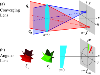
Figure 1: (a) The schematic illustration of the working of a converging lens. The transverse wave-vector modes ${\bm{q}_{1}}$ and ${\bm{q}_{2}}$ with phase profiles $e^{i{\bm{q}_{1}}\cdot\bm{\rho}}$ and $e^{i{\bm{q}_{2}}\cdot\bm{\rho}}$ get localized at separate spatial locations. (b) The schematic illustration of the working of our proposed angular lens. The OAM modes $\ell_{1}$ and $\ell_{2}$ with phase profiles $e^{-i\ell_{1}\phi}$ and $e^{-i\ell_{2}\phi}$ get localized at separate angular positions.

Figure 1(a) illustrates how a converging lens separates out different transverse wave-vector modes. The phase transformation function $T(x,y)$ of a thin converging lens within the paraxial approximation is given by (see Section 5.2 of Ref. Goodman (1996)): $T(x,y)=\exp[-\frac{ik}{2f}(x^{2}+y^{2})]$, where $f$ is the focal length of the lens and where $k=2\pi/\lambda$ with $\lambda$ being the wavelength of light. The lens transforms the transverse wave-vector modes ${\bm{q}_{1}}$ and ${\bm{q}_{2}}$ with phase profiles $e^{i{\bm{q}_{1}}\cdot\bm{\rho}}$ and $e^{i{\bm{q}_{2}}\cdot\bm{\rho}}$, where $|{\bm{q}_{1}}|,|{\bm{q}_{2}}|\ll k$, into localized spots on a transverse plane kept at $z=f$. Figure 1(b) is the schematic illustration of the expected working of an angular lens. We now want to find out the phase transformation function of a lens that performs as depicted in Fig. 1(b).

We begin by noting that the angular-position and the orbital angular momentum (OAM) bases form a Fourier transform pair in much the same way as the transverse position and transverse wave-vector bases do Yao et al. (2006); Jha et al. (2008, 2010). Therefore, it is natural to expect the transformation function of an angular lens to have a quadratic dependence on $\phi$ just as the transformation function of a converging lens has quadratic dependences on $x$ and $y$. However, unlike the transverse position coordinates ($x$, $y$) the cylindrical coordinates ($\rho,\phi$) do not form a two-dimensional Fourier pair. Therefore, it is not straightforward to arrive at an analogous functional dependence on $\rho$. Nevertheless, we take a hint from Ref. Arlt et al. (2001), in which it was shown that an axicon, which has a transformation function given by $e^{i\beta\rho}$ with $\beta$ being a constant, transforms a Laguerre-Gaussian mode into an ultranarrow annulus. With this hint, we take the following as the transformation function $T_{\rm ang}(\rho,\phi)$ of our proposed angular lens:

$$T_{\rm ang}(\rho,\phi)=\exp\left[-i(\alpha\phi^{2}-\beta\rho)\right].$$ (1)

Here $\alpha,\beta$ are two constants and $\phi\in[-\pi,\pi]$ and $\rho\in[0,\infty]$. The thickness function corresponding to the phase transformation function has been plotted in Fig. 2(a).

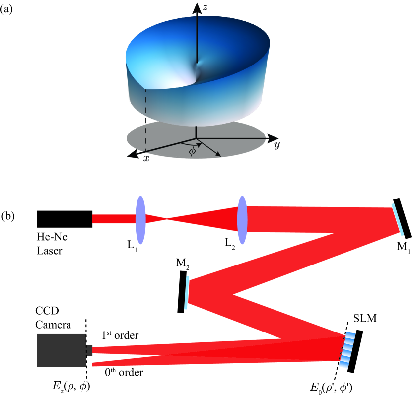
Figure 2: (a) The thickness function of the proposed angular lens. (b) The experimental Setup. SLM is spatial light modulator, L stands for a converging lens, and M stands for a mirror.

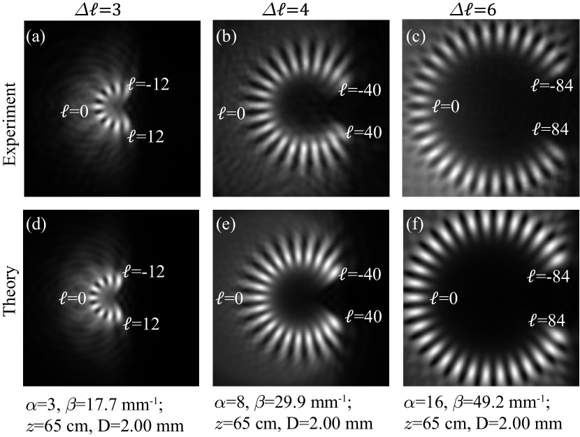
Figure 3: Transformation of constant-intensity OAM modes by the angular lens. (a), (b), and (c) are the combined intensity patterns for various $\ell$ observed at $z=65$ cm. (d)-(f) are the theoretical diffraction patterns as obtained by numerically evaluating the integral in Eq. (2) for the same set of parameters. The screen size in all the above plots is 6.27 mm $\times$ 6.27 mm. A constant background of 250 counts has been subtracted from the each CCD camera pixel.

We now illustrate the workings of our proposed angular lens using the experimental setup shown in Fig. 2(b). An angular lens with the transformation function $T_{\rm ang}(\rho,\phi)$ given by Eq. (1) is placed at $z=0$ and an input field with amplitude $E_{z=0}(\rho^{\prime},\phi^{\prime})$ at $z=0$ is incident on it. The field amplitude $E_{z=z}(\rho,\phi)$ at $z$ is given by the Fresnel diffraction integral Goodman (1996):

$$E_{z=z}(\rho,\phi) =\frac{e^{ikz}}{i\lambda z}e^{i\tfrac{k}{2z}\rho^{2}}\int_{0}^{\infty}\int_{0}^{2\pi}E_{z=0}(\rho^{\prime},\phi^{\prime})$$

$$\times T_{\rm ang}(\rho,\phi)e^{i\tfrac{k}{2z}\rho^{\prime 2}}e^{-i\tfrac{k\rho\rho^{\prime}}{z}\cos(\phi-\phi^{\prime})}\rho^{\prime}d\rho^{\prime}d\phi^{\prime}.$$ (2)

First of all we investigate the transformation properties of our angular lens for input field modes given by $E_{z=0}(\rho^{\prime},\phi^{\prime})=e^{-i\ell\phi^{\prime}}$. Such modes have constant transverse intensity at $z=0$. In our experiment, we generate these modes one by one in a sequential manner, and for each generated mode with a given OAM mode index, we measure the diffracted intensity pattern at $z$. The modes are generated by first expanding our continuous-wave He-Ne laser beam to be 1-cm wide. We then diffract this laser beam from the spatial light modulator (SLM) kept at $z=0$ after putting an appropriate phase pattern on it Mair et al. (2001). We also put a circular aperture of diameter $D=2$ mm onto the SLM so that only a small circular portion of the incoming laser beam undergoes diffraction and thus, to a good approximation, the intensity in the circular portion can be taken as constant. The transformation function corresponding to the angular lens at $z=0$ is also simulated using the same SLM. With an SLM, the diffraction pattern corresponding to the transmission function simulated on it is observed at the first diffraction order; the zeroth diffraction order of an SLM contains mostly the reflected portion of the incoming field and does not contain much information about the transmission function simulated on the SLM Mair et al. (2001); Arrizón et al. (2007). Therefore, we record the transverse intensity at the first SLM diffraction order using a CCD camera placed at $z$. The parameters $\alpha$ and $\beta$ are electronically changed in order to simulate different lenses. By changing $\ell$ in a sequential manner, we generate a range of OAM modes and for each of these modes we measure the diffracted intensity pattern at $z$. After collecting the intensity patterns for various different values of $\ell$, we plot the combined intensity patterns.

Figure 3 shows the combined intensity patterns observed by the CCD camera kept at $z=65$ cm for a range of OAM modes with various $\ell$ and with separation $\Delta\ell$. Figures 3(a), 3(b), and 3(c) show the combined intensity patterns corresponding to $\alpha$ equal to 3, 8, and 16, respectively. In order to consider the two modes as separated we adapt the following resolution criterion: if in the combined two-dimensional intensity plot at $z$, the ratio of the intensity at the minimum located in between the two maxima and that at the maxima is less than about 0.3 then the two modes are resolved. This criterion is much stringent than that of Rayleigh, which allows for ratios up to 0.811. The value of $\beta$ was obtained by optimizing it for a given value of $\alpha$ and $z$ such that we obtain a localized diffraction pattern and the resolution criterion is satisfied. For the three $\alpha$ values, the optimized values of $\beta$ were found to be $17.7$ mm^-1, $29.9$ mm^-1, and $49.2$ mm^-1, respectively. We find that different OAM modes get transformed into diffraction patterns localized at separate angular positions and that as $\alpha$ increases the mode separation $\Delta\ell$ that could be resolved increases as well. For the three $\alpha$ values, we find that modes with separation $\Delta\ell$ equal to 3, 4, and 6 could be resolved. Further, we find that as $\alpha$ increases, the range of modes that can be transformed into localized functions also increases. Figures 3(d)-3(f) show the corresponding theoretical diffraction patterns as obtained by numerically evaluating the integral in Eq. (2) for the same set of parameters. We find an excellent agreement between the theory and experiments.

We note that for the aperture size of $D=2$ mm, $\Delta\ell=3$ is the lowest value. For $\alpha=3$ and $D=2$ mm, $\beta$ cannot be optimized to satisfy the resolution criterion with $\Delta\ell=2$ or $\Delta\ell=1$. This, in fact, is a generic feature of optical elements having finite sizes. For example, a converging lens achieves perfect resolution only when the aperture size is infinite. With finite aperture-sizes, the resolving power of a lens remains limited Goodman (1996). Similar limitation on resolution is also observed in the log-polar mapping based method for sorting OAM modes Bryngdahl (1974a, b). We also note in Fig. 3 that there exists a limit on the maximum value of $\ell$ up to which the angular lens produces localized patterns. Beyond this maximum value the transformation function no longer produces localized patterns. In the figure, we have plotted the results only up to this maximum $\ell$ value. The maximum value of $\ell$ seems to scale as $\alpha$ in the sense that as $\alpha$ increases the maximum value of $\ell$ also increases in a linear manner.

In a converging lens the resolving power is decided by the size of the lens. In our proposed angular lens, the parameter $\alpha$ is playing an analogous role. Both the range of the mode and the minimum separation $\Delta\ell$ that could be resolved depends on the parameter $\alpha$. As $\alpha$ increases, the range of modes that can be resolved increases but the resolution decreases. The parameter $\beta$ is obtained by optimizing it for a given value of $\alpha$ and $z$ such that we obtain a localized diffraction pattern and the resolution criterion is satisfied. The parameter $\beta$ plays a somewhat analogous role as the focal length of a converging lens.

In order to illustrate this analogous property of the $\beta$ parameter, we first recall how the focal length of a converging lens transforms a given input field. We know that for a given input field the focal intensity patterns due to lenses with different focal lengths remain the same except for an overall scaling of the pattern. In the proposed angular lens, the $\beta$ parameter shows an analogous scaling property for fixed $\alpha$ values. In order to show this scaling, let us consider two angular lenses with the same $\alpha$ but with $\beta$ parameters being equal to $\beta_{1}$ and $\beta_{2}$ and the aperture size $D$ being equal to $D_{1}$ and $D_{2}$, respectively. Let us assume that with $\beta_{1}$ and $D_{1}$ the angular lens produces the optimized diffraction pattern at $z=z_{1}$. The field amplitude $E_{z=z_{1}}^{(1)}(\rho,\phi)$ in this case can be written using Eq. (2) as

$$E_{z=z_{1}}^{(1)}(\rho,\phi) =\frac{e^{ikz_{1}}}{i\lambda z_{1}}e^{\tfrac{ik\rho^{2}}{2z_{1}}}\int_{0}^{D_{1}/2}\int_{0}^{2\pi}E_{z=0}(\phi^{\prime})$$

$$\times T_{\rm ang}(\rho,\phi)e^{i\tfrac{k}{2z_{1}}\rho^{\prime 2}}e^{-i\tfrac{k\rho\rho^{\prime}}{z_{1}}\cos(\phi-\phi^{\prime})}\rho^{\prime}d\rho^{\prime}d\phi^{\prime}.$$ (3)

We at once see that since the input field amplitude depends only on $\phi^{\prime}$ the functional form of the intensity due to the first angular lens at $z_{1}$ is equal to that due to the second lens at $z_{2}$, that is,

$$|E_{z=z_{2}}^{(2)}(\rho,\phi)|^{2} =|E_{z=z_{1}}^{(1)}(\rho/a,\phi)|^{2},$$

$$\quad{\rm if}\quad z_{2}=a^{2}z_{1},\ \beta_{2}=\frac{\beta_{1}}{a}\ {\rm and}\ D_{2}=\frac{D_{1}}{a},$$ (4)

for a given constant value of $a$. We thus find that if both $\beta$ and $D$ are decreased by a factor of $a$, one obtains a radially scaled up version of the same diffraction pattern at a propagation distance $z$ that is $a^{2}$ times larger. Figure 4 shows the experimental and theoretical results illustrating this analogous focusing property of the angular lens. The diffraction pattern in Fig. 4(a) is for a lens with $\alpha=8$ and $D=2$ mm, and the $\beta$ parameter was obtained by optimizing it such that we obtain a localized diffraction pattern and the resolution criterion is satisfied. For the results in Figs. 4(b) and 4(c), we chose $z$ to be $100$ cm and $140$ cm respectively and the corresponding $\beta$ and the size of the lens were chosen simply using the scaling in Eq. (4), without any optimization. Figures 4(d)-4(f) are the theoretical diffraction patterns as obtained by numerically evaluating the integral in Eq. (2) for the same set of parameters.

Figure 4: Scaling of diffraction patterns with $z$. (a), (b), and (c) are the combined intensity patterns observed at three $z$ values. (d)-(f) are the theoretical diffraction patterns as obtained by numerically evaluating the integral in Eq. (2) for the same set of parameters. The screen size in all the above plots is 6.27 mm $\times$ 6.27 mm. A constant background of 250 counts has been subtracted from the each CCD camera pixel.

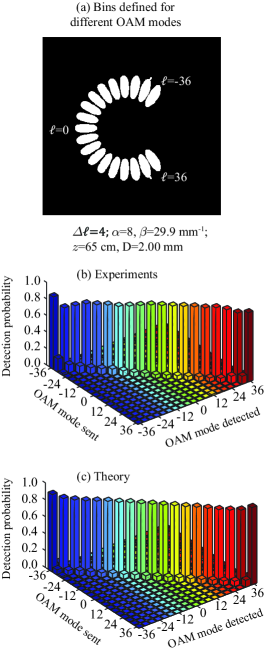
Figure 5: Cross-talk analysis. (a) The theoretically defined bins for different OAM modes. (b) Experimental detection probability of the 19 input OAM modes. (c) The theoretical detection probability of the 19 input OAM modes.

Our results so far have illustrated how our proposed angular lens transforms different OAM modes into localized spots at separated angular positions on a transverse plane. We have shown that our angular lens separates out OAM modes in a manner analogous to how a converging lens separates out transverse wave-vector modes at the focal plane. We next quantify the resolving power of our angular lens in terms of its use as an OAM sorter. For this purpose, we adopt the overall procedure of Refs. Mirhosseini et al. (2013); Bozinovic et al. (2013); Huang et al. (2015) and calculate the cross-talk for the set of lens parameters reported in figs. 3(b) and 3(c). First, we divide the detection area on the CCD into 19 non-overlapping spatial bins so as to define a detection bin for each OAM mode with index ranging from $\ell=-36$ to $\ell=36$ with separation $\Delta\ell=4$. In order to define these bins, we have used the diffracted intensity expression of Eq. (2) for the given set of lens parameters and labeled a given set of pixels as one bin if the set of pixels have at least 25% of the intensity of the most-intense pixel. The pixels having less than 25% intensity do not define any bin. The spatial bins defined this way have been plotted in fig. 5(a). We then send a known OAM mode through our system and record the intensity in each of the 19 spatial bins. We repeat this for all the 19 input OAM modes and plot the detection probability for each spatial bin in fig. 5(b). Figure 5(c) shows the theoretical detection probability for each spatial bins. The cross-talk for a given mode has been defined as the fraction of the input intensity collected in spatial bins other than the one meant for the given mode. The experimental cross-talk averaged over all the 19 modes turns out to be 16.5%. The theoretically calculated average cross-talk come out to be 12.5%. We note that, in the context of log-polar mapping based method Berkhout et al. (2010); Lavery et al. (2012); O’Sullivan et al. (2012); Mirhosseini et al. (2013), when the method is used in combination with the idea of beam copying Romero and Dickey (2007) modes with $\Delta\ell=1$ O’Sullivan et al. (2012); Mirhosseini et al. (2013) can be separated with less than 10% cross-talk. We believe that similar beam-copying techniques can also be employed to enhance the resolving power of our angular lens. Moreover, as opposed to the log-polar based methods, which require several elements for its implementation and are thus limited by the severe transmission loss Mirhosseini et al. (2013) in the system, our angular lens is a single phase-only element and so when realized using a single glass element, instead on of an SLM, the transmission loss can be made negligibly small.

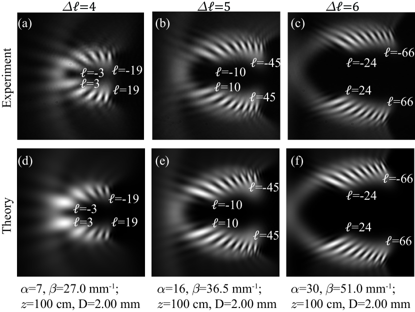
Figure 6: Transformation of LG modes by the proposed angular lens. (a), (b), and (c) are the combined intensity patterns for various $\ell$ with $p=0$ observed at $z=100$ cm. (d)-(f) are the theoretical diffraction patterns as obtained by numerically evaluating the integral in Eq. (2) for the same set of parameters. The screen size in all the above plots is 5.63 mm $\times$ 5.63 mm. A constant background of 170 counts has been subtracted from the each CCD camera pixel.

III Action of angular lens on LG modes

Next, we study the action of our angular lens on the Laguerre-Gaussian (LG) modes, which are the exact propagating solutions of the paraxial Helmholtz equation and are denoted by two indices, $\ell$ and $p$. The index $\ell$ decides the OAM content and the index $p$ decides the radial intensity distribution. We produce LG modes using the method by Arrizón et al. Arrizón et al. (2007). Figure 6 shows the combined intensity patterns observed by the CCD camera kept at $z=100$ cm when a range of LG modes with $p=0$ and with separation $\Delta\ell$ were sequentially incident on angular lenses having various sets of values for $\alpha$ and $\beta$. Figures 6(a), 6(b), and 6(c) show the combined intensity patterns corresponding to $\alpha$ being equal to 7, 16, and 30, respectively. As before, for a given value of $\alpha$, the value of $\beta$ was obtained by optimizing it such that we obtain a localized diffraction pattern and the resolution criterion is satisfied. The values of $\beta$ for the three $\alpha$ values were found to be $27.0$ mm^-1, $36.5$ mm^-1, and $51.0$ mm^-1, respectively. The mode separation $\Delta\ell$ that could be resolved for the three $\alpha$ values, were 4, 5, and 6, respectively. Figures 6(d)-6(f) show the theoretical diffraction patterns as obtained by numerically evaluating the integral in Eq. (2) for the same set of parameters. Although the proposed angular lens is able to separate out the LG modes, it does not have all the analogous feature as in the case of flat-intensity OAM modes. More specifically, we do not see the same scaling as is seen in the case of constant-intensity OAM modes through Eq. (3) and Eq. (4). This is because in this case the input field amplitude depends on both $\rho^{\prime}$ and $\phi^{\prime}$ and therefore Eq. (3) does not show the same scaling.

IV Summary

In conclusion, we have proposed a single phase-only optical element that can transform different OAM modes into localized patterns at separated angular positions on a transverse plane. Using an SLM, we have experimentally demonstrated the working of our proposed angular lens for two different types of OAM modes. For constant-intensity OAM modes, our angular lens works in a manner analogous to how a converging lens works for transverse wave-vector modes. Even for the LG modes, our proposed angular lens is able to separate out the modes based on their OAM mode index. In several situations there are techniques that are employed to increase the resolving power of an optical element beyond its usual diffraction limit. For example, in the context of log-polar mapping based method Berkhout et al. (2010); Lavery et al. (2012); O’Sullivan et al. (2012); Mirhosseini et al. (2013), it was shown that when the method is used in combination with the idea of beam copying Romero and Dickey (2007) it can separate out modes with $\Delta\ell=1$ O’Sullivan et al. (2012); Mirhosseini et al. (2013). We believe that similar techniques can also be employed to enhance the resolving power of our angular lens. Since the proposed angular lens is purely a phase-only element and works at any light level, we expect our work to have several important implications for OAM-based communication protocols in both classical Wang et al. (2012); Bozinovic et al. (2013); Yan et al. (2014) and quantum domains Karimipour et al. (2002); Cerf et al. (2002); Nikolopoulos et al. (2006); Fujiwara et al. (2003); Cortese (2004); Ralph et al. (2007); Lanyon et al. (2009); Jha et al. (2011); Kaszlikowski et al. (2000); Collins et al. (2002); Vértesi et al. (2010); Leach et al. (2009).

Funding

The initiation grant no. IITK /PHY /20130008 from Indian Institute of Technology (IIT) Kanpur, India; The research grant no. EMR/2015/001931 from the Science and Engineering Research Board (SERB), Department of Science and Technology, Government of India; The grant no. 1454931 from the Directorate for Mathematical and Physical Sciences, National Science Foundation, USA.

References

- Goodman (1996) J. Goodman, Introduction to Fourier Optics (McGraw Hill, New York, 1996), 2nd ed.
- Born and Wolf (1999) M. Born and E. Wolf, Principles of Optics (Cambridge University Press, Cambridge, 1999), 7th ed.
- Allen et al. (1992) L. Allen, M. W. Beijersbergen, R. J. C. Spreeuw, and J. P. Woerdman, Phys. Rev. A 45, 8185 (1992).
- Wang et al. (2012) J. Wang, J.-Y. Yang, I. M. Fazal, N. Ahmed, Y. Yan, H. Huang, Y. Ren, Y. Yue, S. Dolinar, M. Tur, et al., Nat Photon 6, 488 (2012), ISSN 1749-4885.
- Bozinovic et al. (2013) N. Bozinovic, Y. Yue, Y. Ren, M. Tur, P. Kristensen, H. Huang, A. E. Willner, and S. Ramachandran, Science 340, 1545 (2013), ISSN 0036-8075.
- Yan et al. (2014) Y. Yan, G. Xie, M. P. J. Lavery, H. Huang, N. Ahmed, C. Bao, Y. Ren, Y. Cao, L. Li, Z. Zhao, et al., Nature Communications 5, 4876 (2014).
- Karimipour et al. (2002) V. Karimipour, A. Bahraminasab, and S. Bagherinezhad, Phys. Rev. A 65, 052331 (2002).
- Cerf et al. (2002) N. J. Cerf, M. Bourennane, A. Karlsson, and N. Gisin, Phys. Rev. Lett. 88, 127902 (2002).
- Nikolopoulos et al. (2006) G. M. Nikolopoulos, K. S. Ranade, and G. Alber, Phys. Rev. A 73, 032325 (2006).
- Fujiwara et al. (2003) M. Fujiwara, M. Takeoka, J. Mizuno, and M. Sasaki, Phys. Rev. Lett. 90, 167906 (2003).
- Cortese (2004) J. Cortese, Phys. Rev. A 69, 022302 (2004).
- Ralph et al. (2007) T. C. Ralph, K. J. Resch, and A. Gilchrist, Phys. Rev. A 75, 022313 (2007).
- Lanyon et al. (2009) B. P. Lanyon, M. Barbieri, M. P. Almeida, T. Jennewein, T. C. Ralph, K. J. Resch, G. J. Pryde, J. L. O/’Brien, A. Gilchrist, and A. G. White, Nat Phys 5, 134 (2009), ISSN 1745-2473.
- Jha et al. (2011) A. K. Jha, G. S. Agarwal, and R. W. Boyd, Phys. Rev. A 83, 053829 (2011).
- Kaszlikowski et al. (2000) D. Kaszlikowski, P. Gnaciński, M. Żukowski, W. Miklaszewski, and A. Zeilinger, Phys. Rev. Lett. 85, 4418 (2000).
- Collins et al. (2002) D. Collins, N. Gisin, N. Linden, S. Massar, and S. Popescu, Phys. Rev. Lett. 88, 040404 (2002).
- Vértesi et al. (2010) T. Vértesi, S. Pironio, and N. Brunner, Phys. Rev. Lett. 104, 060401 (2010).
- Leach et al. (2009) J. Leach, B. Jack, J. Romero, M. Ritsch-Marte, R. W. Boyd, A. K. Jha, S. M. Barnett, S. Franke-Arnold, and M. J. Padgett, Opt. Express 17, 8287 (2009).
- Mair et al. (2001) A. Mair, A. Vaziri, G. Weihs, and A. Zeilinger, Nature 412, 313 (2001).
- Gibson et al. (2004) G. Gibson, J. Courtial, M. J. Padgett, M. Vasnetsov, V. Pas’ko, S. M. Barnett, and S. Franke-Arnold, Opt. Express 12, 5448 (2004).
- Gruneisen et al. (2011) M. T. Gruneisen, R. C. Dymale, K. E. Stoltenberg, and N. Steinhoff, New Journal of Physics 13, 083030 (2011).
- Leach et al. (2002) J. Leach, M. J. Padgett, S. M. Barnett, S. Franke-Arnold, and J. Courtial, Phys. Rev. Lett. 88, 257901 (2002).
- Leach et al. (2004) J. Leach, J. Courtial, K. Skeldon, S. M. Barnett, S. Franke-Arnold, and M. J. Padgett, Phys. Rev. Lett. 92, 013601 (2004).
- Vasnetsov et al. (2003) M. Vasnetsov, J. Torres, D. Petrov, and L. Torner, Optics letters 28, 2285 (2003).
- Courtial et al. (1998) J. Courtial, D. A. Robertson, K. Dholakia, L. Allen, and M. J. Padgett, Phys. Rev. Lett. 81, 4828 (1998).
- Berkhout et al. (2010) G. C. Berkhout, M. P. Lavery, J. Courtial, M. W. Beijersbergen, and M. J. Padgett, Phys. Rev. Lett. 105, 153601 (2010).
- Lavery et al. (2012) M. P. Lavery, D. J. Robertson, G. C. Berkhout, G. D. Love, M. J. Padgett, and J. Courtial, Optics express 20, 2110 (2012).
- Lightman et al. (2017) S. Lightman, G. Hurvitz, R. Gvishi, and A. Arie, Optica 4, 605 (2017).
- Bryngdahl (1974a) O. Bryngdahl, JOSA 64, 1092 (1974a).
- Bryngdahl (1974b) O. Bryngdahl, Optics Communications 10, 164 (1974b).
- Yao et al. (2006) E. Yao, S. Franke-Arnold, J. Courtial, S. Barnett, and M. Padgett, Opt. Express 14, 9071 (2006).
- Jha et al. (2008) A. K. Jha, B. Jack, E. Yao, J. Leach, R. W. Boyd, G. S. Buller, S. M. Barnett, S. Franke-Arnold, and M. J. Padgett, Phys. Rev. A 78, 043810 (pages 4) (2008).
- Jha et al. (2010) A. K. Jha, J. Leach, B. Jack, S. Franke-Arnold, S. M. Barnett, R. W. Boyd, and M. J. Padgett, Phys. Rev. Lett. 104, 010501 (2010).
- Arlt et al. (2001) J. Arlt, R. Kuhn, and K. Dholakia, journal of modern optics 48, 783 (2001).
- Arrizón et al. (2007) V. Arrizón, U. Ruiz, R. Carrada, and L. A. González, J. Opt. Soc. Am. A 24, 3500 (2007).
- Mirhosseini et al. (2013) M. Mirhosseini, M. Malik, Z. Shi, and R. W. Boyd, Nature communications 4 (2013).
- Huang et al. (2015) H. Huang, G. Milione, M. P. Lavery, G. Xie, Y. Ren, Y. Cao, N. Ahmed, T. A. Nguyen, D. A. Nolan, M.-J. Li, et al., Scientific reports 5, 14931 (2015).
- O’Sullivan et al. (2012) M. N. O’Sullivan, M. Mirhosseini, M. Malik, and R. W. Boyd, Optics express 20, 24444 (2012).
- Romero and Dickey (2007) L. A. Romero and F. M. Dickey, JOSA A 24, 2280 (2007).