Constraints on physical reality arising from a formalization of knowledge

Abstract

There are (at least) four ways that an agent can acquire information concerning the state of the universe: via observation, control, prediction, and via retrodiction, i.e., memory. Each of these four ways of acquiring information seems to rely on a different kind of physical device (resp., an observation device, a control device, etc.). However it turns out that certain mathematical structure is common to those four types of device. Any device that possesses a certain subset of that structure is known as an “inference device” (ID).

Here I review some of the properties of IDs, including their relation with Turing machines, and (more loosely) quantum mechanics. I also review the bounds of the joint abilities of any set of IDs to know facts about the physical universe that contains them. These bounds constrain the possible properties of any universe that contains agents who can acquire information concerning that universe.

I then extend this previous work on IDs, by adding to the definition of IDs some of the other mathematical structure that is common to the four ways of acquiring information about the universe but is not captured in the (minimal) definition of IDs. I discuss these extensions of IDs in the context of epistemic logic (especially possible worlds formalisms like Kripke structures and Aumann structures). In particular, I show that these extensions of IDs are not subject to the problem of logical omniscience that plagues many previously studied forms of epistemic logic.

I Introduction

Ever since Wheeler discussed “it from bit” whee90 , there has been great interest in what constraints on the properties of the universe can be derived using some appropriate mathematical formulation of information. Some of this work relies on Shannon information theory caticha2011entropic ; goyal2010information ; goyal2012information ; hartle2005physics , and some of it on Fisher information theory frieden2004science . There has also been work on this topic that focuses on the processing of information, i.e., that views the universe through the lens of Turing machine (TM) theory lloyd1990valuable ; chaitin2004algorithmic ; zure89a ; zure89b ; zurek1990complexity ; zenil2012computable ; lloyd2006programming ; schmidhuber2000algorithmic ; zuse1969rechnender .

Here I adopt a different approach. I focus on the fact that information concerning the state of the universe typically is held by some agent embedded in that universe. For example, we cannot speak of Shannon information without specifying probability distributions — which reflect the uncertainty of some specific agent concerning the state of the universe that contains them (e.g., uncertainty of a scientist making a prediction).

This leads us to analyze how an agent can acquire information concerning the state of the world. That is the topic of this paper, as described in the remainder of this introduction.

I.1 Inference devices

There are (at least) four ways an agent can acquire some information concerning the universe in which it is embedded: via an observation device, via a control device, via a prediction device, and via a memory device, i.e., a “retrodiction” device. It turns out that there is some mathematical structure shared by all such information-acquiring devices. Devices with that structure are called “Inference Devices” (IDs) wolp01 ; wolp08b ; wolp10 ; bind08 .

In the first section of this paper I present two examples of how an agent can acquire information about the universe that contains them, illustrating that in both examples the agent has the mathematical structure of an ID. I then present some of the more elementary impossibility results concerning IDs. These results place strong constraints on what information about a universe can be jointly held by different IDs embedded in that universe. Importantly, these constraints arise only from the definition of IDs, without any assumptions about the laws of the universe containing the IDs; they hold in any universe that allows agents that have information about that universe. In particular, they would hold even in a classical, finite universe, with no chaotic processes. They would also hold even in a universe with agents who have super-Turing computation abilities, can transmit information at super-luminal rates, etc. It is worth noting as well that these impossibility theorems hold even though there is no sense in which IDs have the ability of self-reference.

After these preliminaries I present some of the connections between the theory of IDs and the theory of Turing Machines. In particular I analyze some of the properties of an ID version of universal Turing machines and of an ID version of Kolmogorov complexity lloyd1990valuable ; chaitin2004algorithmic ; zure89a ; zure89b ; zurek1990complexity ; zenil2012computable ; lloyd2006programming ; schmidhuber2000algorithmic ; zuse1969rechnender . I show that the ID versions of those quantities obey many of the familiar results of Turing machine theory (e.g., the invariance theorem of TM theory).

I then consider one way to extend the theory of IDs to the case where there is a probability distribution over the states of the universe, so that no information is ever 100% guaranteed to be true. In particular, I present a result concerning the products of probabilities of error of two separate IDs, a result which is formally similar to the Heisenberg uncertainty principle.

These results all concern subsets of an entire universe, e.g., one or two IDs embedded in a larger universe. However we can expand the scope to an entire universe. The idea is to define a “universe”, with whatever associated laws of physics, to be a set of physical systems and IDs (e.g., a set of scientists), where the IDs can have information concerning those physical systems and / or one another. Adopting this approach, I use the theory of IDs to derive impossibility results concerning the nature of the entire universe.

I.2 Inference devices and epistemic logic

Most of the results presented to this point in the paper have appeared before, albeit in a more complicated, less transparent formalism than the one used here wolp01 ; wolp08b ; wolp10 ; bind08 . In the last sections of the paper I present new results. These all involve an extension of IDs, one that includes some of the features that are shared by the four ways for an agent to acquire information (observation, control, prediction and memory) but that are not in the original definition of IDs.

I show that this strengthened version of IDs has a close relation to the various ways of formalizing “knowledge” that are considered in epistemic logic fagin2004reasoning ; aaronson2013philosophers ; parikh1987knowledge ; zalta2003stanford . However the ID-based theory of knowledge is not subject to what is perhaps the major problem of these earlier ways of formalizing knowledge, the problem of logical omniscience.

To explain that problem, it is easiest to work with the event-based formulation of epistemic logic pioneered by Aumann aumann1976agreeing ; auma99 ; aubr95 ; futi91 ; bibr88 . In this formulation we start with a space $U$ of possible states of the entire universe across all time. (In the literature this is typically called a set of “possible worlds”.) An event is defined as a subset of $U$. For example, let $U$ be a set of all possible histories of the universe across all time and space. Then the event {there are no clouds in the sky in London during January 1, 2000} is all $u\in U$ such that {there are no clouds in the sky in London during January 1, 2000}. Belief by an agent concerning the universe is formalized in terms of a partition of $U$, which is called an Aumann structure and an associated belief operator $B:U\rightarrow\{R_{i}\}$. This is supposed to represent the intuition that in any universe $u$, the agent believes that an event $E\subset U$ holds iff $B(u)\subseteq E$. Knowledge is then defined as true belief, i.e., a belief operator $K$ with the property that $u\in K(u)$ for all $u\in U$ fagin2004reasoning . Similarly, in the event-based framework we say that “an agentknows event $E$ in world $u\in U$” if $E$ holds for all worlds that the agent believes are possible when the actual world is $u$. So an agent knows $E$ at $u$ if for their knowledge operator, $K(u)\subseteq E$.

Now suppose that some event $E$ implies some event $E^{\prime}$, i.e., $E^{\prime}\supseteq E$. This means that under the event-based definition of knowledge, if agent $i$ knows event $E$ in world $u$, $E^{\prime}$ is also true in world $u$ — and agent $i$ knows event $E^{\prime}$ in world $u$. Generalizing, the agent cannot know a set of facts without knowing all logical implications of those facts. This is known as the property of logical omniscience. As an example of this property, suppose that someone multiplies two huge prime numbers and then (honestly) tells that product to the agent — so that the agent knows that product. Then since that product logically implies its unique prime factorization, under the event-based framework the agent must “know” the two prime numbers, independent of any considerations of whether they have a computer to help them do calculations. This of course is absurd.

This problem of logical omniscience plagues possible-worlds models of epistemic logic like those based on Aumann structures. Some extensions to possible-worlds models have been proposed to address this problem, e.g., bounds on the computational powers of the agent aaronson2013philosophers , assuming that the agent reasons illogically fagin2004reasoning , and a set of related “impossible possible worlds” restrictions on the nature of the agent fagin2004reasoning ; aaronson2013philosophers ; parikh1987knowledge ; zalta2003stanford . However none of these has proven broadly convincing.

There are other difficulties with the event-based formalization of knowledge. In that framework, by simply defining the “knowledge operator” of a rock on the moon appropriately, we would say that the rock “knows” whether it is in sunlight or not (for example by having its knowledge operator pick sets of states of the universe based on the temperature of that rock). This pathology is due to the fact that the definition of knowledge operators in the event-based framework does not reflect the fact that knowledge is held by a sentient agent. Specifically, any sentient agent that knows something about the universe is able to correctly answer arbitrary questions about what they know, either implicitly or explicitly. (Note that a lunar rock cannot answer such questions.) However there is nothing in the formal structure of Aumann structures, Kripke structures, or the like that involves the ability of agents to correctly answer questions.

The ID framework is concerned precisely with such ability of an agent to answer questions about the information they have. As a result, in the extension of the ID framework into a full-fledged theory of knowledge, we cannot say that a rock on the moon “knows” whether it is in sunlight. Moreover, the ID-based theory of knowledge avoids the problem of logical omniscience. Specifically, in the ID-based formalization of knowledge, if an agent knows some fact $A$, and knows that $A$ implies $B$, then $B$ is true — but the agent may not know that.

None of the results below are difficult to prove; some of the proofs, especially those of the “Laplace demon theorems”, are almost trivial. (The interest is the implications of the inference device axioms for metaphysics and epistemology, not the math needed to derive those implications.) Nonetheless, the interested reader can find all proofs that are not given below in wolp08b .

II Inference Devices

In this section I review the elementary properties of inference devices, mathematical structures that are shared by the processes of observation, prediction, recall and control wolp01 ; wolp08b ; wolp10 ; bind08 . These results are proven by extending Epimenides’ paradox to apply to novel scenarios. Results relying on more sophisticated mathematics, some of them new, are presented the following section.

II.1 Observation, prediction, recall and control of the physical world

I begin with two examples that motivate the formal definition of inference devices. The first is an example of an agent making a correct observation about the current state of some physical variable.

Example 1.

Consider an agent who claims to be able to observe $S(t_{2})$, the value of some physical variable at time $t_{2}$. If the agent’s claim is correct, then for any question of the form “Does $S(t_{2})=L$?”, the agent is able to consider that question at some $t_{1}<t_{2}$, observe $S(t_{2})$, and then at some $t_{3}>t_{2}$ provide the answer “yes” if $S(t_{2})=L$, and the answer “no” otherwise. In other words, she can correctly pose any such binary question to herself at $t_{1}$, and correctly say what the answer is at $t_{3}$.

To formalize this, let $U$ refer to a set of possible histories of an entire universe across all time, where each $u\in U$ has the following properties:

1. $u$ is consistent with the laws of physics,

2. In $u$, the agent is alive and of sound mind throughout the time interval $[t_{1},t_{3}]$, and the system $S$ exists at the time $t_{2}$,

3. In $u$, at time $t_{1}$ the agent considers some $L$-indexed question $q$ of the form “Does $S(t_{2})=L$?”,

4. In $u$, the agent observes $S(t_{2})$,

5. In $u$, at time $t_{3}$ the agent uses that observation to provide her (binary) answer to $q$, and believes that answer to be correct.

The agent’s claim is that for any question $q$ of the form “Does $S(t_{2})=L$?”, the laws of physics imply that for all $u$ in the subset of $U$ where at $t_{1}$ the agent considers $q$, it must be that the agent provides the correct answer to $q$ at $t_{3}$. Any prior knowledge concerning the history that the agent relies on to make this claim is embodied in the set $U$.

The value $S(t_{2})$ is a function of the actual history of the entire universe, $u\in U$. Write that function as $\Gamma(u)$, with image $\Gamma(U)$. Similarly, the question the agent has in her brain at $t_{1}$, together with the time $t_{1}$ state of any observation apparatus she will use, is a function of $u$. Write that function as $X(u)$. Finally, the binary answer the agent provides at $t_{3}$ is a function of the state of her brain at $t_{3}$, and therefore it too is a function of $u$. Write that binary-valued function giving her answer as $Y(u)$.

Note that since $U$ embodies the laws of physics, in particular it embodies all neurological processes in the agent (e.g., her asking and answering questions), all physical characteristics of $S$, etc.

So as far as this observation is concerned, the agent is just a pair of functions $(X,Y)$, both with the domain $U$ defined above, where $Y$ has the range $\{-1,1\}$. A necessary condition for us to say that the agent can “observe $S(t_{2})$” is that for any $\gamma\in\Gamma(U)$, there is some associated $X$ value $x$ such that for all $u\in U$, so long as $X(u)=x$, it follows that $Y(u)=1$ iff $\Gamma(u)=\gamma$.

I now present an example of an agent making a correct prediction about the future state of some physical variable.

Example 2.

Now consider an agent who claims to be able to predict $S(t_{3})$, the value of some physical variable at time $t_{3}$. If the agent’s claim is correct, then for any question of the form “Does $S(t_{3})=L$?”, the agent is able to consider that question at some time $t_{1}<t_{3}$, and produce an answer at some time $t_{2}\in(t_{1},t_{3})$, where the answer is “yes” if $S(t_{3})=L$ and “no” otherwise. So loosely speaking, if the agent’s claim is correct, then for any $L$, by their considering the appropriate question at $t_{1}$, they can generate the correct answer to any question of the form “Does $S(t_{3})=L$?” at $t_{2}<t_{3}$.

To formalize this, let $U$ refer to a set of possible histories of an entire universe across all time, where each $u\in U$ has the following properties:

1. $u$ is consistent with the laws of physics,

2. In $u$, the agent exists throughout the interval $[t_{1},t_{2}]$, and the system $S$ exists at $t_{3}$,

3. In $u$, at $t_{1}$ the agent considers some question $q$ of the form “Does $S(t_{3})=L$?”,

4. In $u$, at $t_{2}$ the agent provides his (binary) answer to $q$ and believes that answer to be correct.

The agent’s claim is that for any question $q$ of the form “Does $S(t_{3})=L$?”, the laws of physics imply that for all $u$ in the restricted set $U$ such that at $t_{1}$ the agent considers $q$, it must be that the agent provides the correct answer to $q$ at $t_{2}$.

The value $S(t_{3})$ is a function of the actual history of the entire universe, $u\in U$. Write that function as $\Gamma(u)$, with image $\Gamma(U)$. Similarly, the question the agent considers at $t_{1}$ is a function of the state of his brain at $t_{1}$, and therefore is also a function of $u$. Write that function as $X(u)$. Finally, the binary answer the agent provides at $t_{2}$ is a function of the state of his brain at $t_{2}$, and therefore it too is a function of of $u$. Write that function as $Y(u)$.

So as far as this prediction is concerned, the agent is just a pair of functions $(X,Y)$, both with the domain $U$ defined above, where $Y$ has the range $\{-1,1\}$. The agent can indeed predict $S(t_{3})$ if for the space defined above $U$, for any $\gamma\in\Gamma(U)$, there is some associated $X$ value $x$ such that, no matter what precise history $u\in U$ we are in, due to the laws of physics, if $X(u)=x$ then the associated $Y(u)$ equals $1$ iff $\Gamma(u)=\gamma$.

Evidently, agents who perform observation and those who perform prediction are described in part by a shared mathematical structure, involving functions $X$ and $Y$ defined over the same space $U$ of all possible histories of the universe across all time. As formalized below, I refer to any such pair $(X,Y)$ as an “inference device”. Say that for some function $\Gamma$ defined over $U$, for any $\gamma\in\Gamma(U)$, there is some associated $X$ value $x$ such that, no matter what precise history $u\in U$ we are in, due to the laws of physics, if $X(u)=x$ then the associated $Y(u)$ equals $1$ iff $\Gamma(u)=\gamma$. Then I will say that the device $(X,Y)$ “infers” $\Gamma$.

See wolp08b for a more detailed elaboration of the examples given above of observation and prediction in terms of inference devices. Arguably to fully formalize each of these phenomena there should be additional structure beyond that defining inference devices. (See App. B. of wolp08b .) Most such additional structure is left for future research. However, one particular part of such additional structure is investigated below, in the discussion of “physical knowledge”.

In addition to considering observation and prediction, it is also shown in wolp08b that a system that remembers the past is an inference device that infers an appropriate function $\Gamma(u)$. wolp08b also shows that a device that controls a physical variable is an inference device that infers an appropriate function $\Gamma(u)$. All of this analysis holds even if what is observed / predicted / remembered / controlled is not the answer to a question of the form, “Does $S(t)=L$?”, but instead an answer to question of the form, “is $S(t)$ more property $A$ than it is property $B$?” or of the form, “is $S(t)$ more property $A$ than $S^{\prime}(t)$ is?”

In the sequel I will sometimes consider situations involving multiple inference devices, $(X_{1},Y_{1}),(X_{2},Y_{2}),\ldots$, with associated domains $U_{1},U_{2},\ldots$. For example, I will consider scenarios where agents try to observe one another. In such situations, when referring to “$U$”, I implicitly mean $\cap_{i}U_{i}$, implicitly restrict the domain of all $X_{i},Y_{i}$ to $U$, and implicitly assume that the codomain of each such restricted $Y_{i}$ is binary.

II.2 Notation and terminology

To formalize the preceding considerations, I first fix some notation. I will take the set of binary numbers $\mathbb{B}$ to equal $\{-1,1\}$. In the canonical case where $U$ is the set of all possible histories of the entire universe across all space and time, the value of any specific physical variable is specified by a subset of the components of a full vector $u\in U$. (For example, the variable of the speed of a particular particle in a particular intertial frame at a particular time is given by a subset of the components of $u$.) So any such variable is just a function over $U$. Bearing this in mind, for any function $\Gamma$ with domain $U$, I will write the image of $U$ under $\Gamma$ as $\Gamma(U)$, i.e., for the set of possible values of some physical variable. I will also sometimes abuse this notation with a sort of “set-valued function” shorthand, and so for example write $\Gamma(V)=1$ for some $V\subset U$ iff $\Gamma(u)=1\;\forall u\in V$. On the other hand, for the special case where the function over $U$ is a measure, I use conventional shorthand from measure theory. For example, if $P$ is a probability distribution over $U$ and $V\subset U$, I write $P(V)$ as shorthand for $\sum_{u\in V}P(u)$.

For any function $\Gamma$ with domain $U$ that I will consider, I implicitly assume that the entire set $\Gamma(U)$ contains at least two distinct elements. For any (potentially infinite) set $R$, $|R|$ is the cardinality of $R$.

Given a function $\Gamma$ with domain $U$, I write the partition of $U$ given by $\Gamma^{-1}$ as $\overline{\Gamma}$, i.e.,

$${\overline{\Gamma}} \equiv \{\{u:\Gamma(u)=\gamma\}:\gamma\in\Gamma(U)\}$$ (1)

I say that two functions $\Gamma_{1}$ and $\Gamma_{2}$ with the same domain $U$ are (functionally) equivalent iff the inverse functions $\Gamma_{1}^{-1}$ and $\Gamma_{2}^{-1}$ induce the same partitions of $U$, i.e., iff ${\overline{\Gamma_{1}}}={\overline{\Gamma_{2}}}$.

Recall that a partition $A$ over a space $U$ is a refinement of a partition $B$ over $U$ iff every $a\in A$ is a subset of some $b\in B$. If $A$ is a refinement of $B$, then for every $b\in B$ there is an $a\in A$ that is a subset of $b$. Some of the elementary properties of refinement will be used below, and so I now review them. First, two partitions $A$ and $B$ are refinements of each other iff $A=B$. Say a partition $A$ is finite and a refinement of a partition $B$. Then $|A|=|B|$ iff $A=B$. For any two functions $A$ and $B$ with domain $U$, I will say that “$A$ refines $B$” if ${\overline{A}}$ is a refinement of $\overline{B}$. Similarly, for any $R\subset U$ and function $A$, I will say that “$R$ refines $A$” (or “$A$ is refined by $R$”) if $R$ is a subset of some element of $\overline{A}$.

I write the characteristic function of any set $R\subseteq U$ as the binary-valued function

$$\mathcal{X}_{R}(u)=1\Leftrightarrow u\in R$$ (2)

As shorthand I will sometimes treat functions as equivalent to one of the values in their image. So for example expressions like “$\Gamma_{1}=\Gamma_{2}\Rightarrow\Gamma_{3}=1$” means ‘$`\forall u\in U$ such that $\Gamma_{1}(u)=\Gamma_{2}(u)$, $\Gamma_{3}(u)=1$”.

To simplify terminology, rather than referring to Kronecker delta functions (and / or Dirac delta functions) throughout, I will refer to a probe of a variable $V$, by which I mean any function over $U$ parametrized by a $v\in V$ of the form

$$\delta_{v}(v^{\prime})=\begin{cases}1&\text{ if $v=v^{\prime}$}\\ -1&\text{ otherwise.}\end{cases}$$ (3)

$\forall v^{\prime}\in V$. Given a function $\Gamma$ with domain $U$ I sometimes write $\delta_{\gamma}(\Gamma)$ as shorthand for the function $u\in U\rightarrow\delta_{\gamma}(\Gamma(u))$. When I don’t want to specify the subscript $\gamma$ of a probe, I sometimes generically write $\delta$. I write ${\mathcal{P}}(\Gamma)$ to indicate the set of all probes over $\Gamma(U)$.

II.3 Weak inference

I now review some results that place severe restrictions on what a physical agent can predict / observe / control / remember and be guaranteed to be correct (in that prediction / observation / control / memory). To begin, I formalize the concept of an “inference device” introduced in the previous subsection.

Definition 1.

An (inference) device over a set $U$ is a pair of functions $(X,Y)$, both with domain $U$. $Y$ is called the conclusion function of the device, and is surjective onto $\mathbb{B}$. $X$ is called the setup function of the device.

Given some function $\Gamma$ with domain $U$ and some $\gamma\in\Gamma(U)$, we are interested in setting up a device so that it is assured of correctly answering whether $\Gamma(u)=\gamma$ for the actual universe $u$. Motivated by the examples above, I will formalize this with the condition that $Y(u)=1$ iff $\Gamma(u)=\gamma$ for all $u$ that are consistent with some associated setup value $x$ of the device, i.e., such that $X(u)=x$ for some $x$. If this condition holds, then setting up the device to have setup value $x$ guarantees that the device will make the correct conclusion concerning whether $\Gamma(u)=\gamma$. (Hence the terms “setup function” and “conclusion function” in Def. 1.)

We can formalize this as follows:

Definition 2.

Let $\Gamma$ be a function over $U$ such that $|\Gamma(U)|\geq 2$. A device ${\mathcal{D}}$ (weakly) infers $\Gamma$ iff $\forall\gamma\in\Gamma(U)$, $\exists x\in X(U)$ such that $\forall u\in U,X(u)=x\Rightarrow Y(u)=\delta_{\gamma}({\Gamma(u)})$.

If ${\mathcal{D}}$ infers $\Gamma$, I write ${\mathcal{D}}>\Gamma$. I say that a device ${\mathcal{D}}$ infers a set of functions if it infers every function in that set.

The following semi-formal example illustrates a scenario in which weak inference holds, and a related scenario in which it doesn’t hold.

Example 3.

A scenario in which weak inference holds is illustrated in Fig. 1. In this example, for simplicity determinism is assumed. The full rectangle, including both colored rectangles, indicates the set of all possible histories of the universe across all time, $U$ (i.e., the set of all “states of the world”, in the language of epistemology). In this example the function $\Gamma$ is whether the sky will (not) be cloudy at noon (at Greenwich, say). Since the ID is embedded in the universe, the precise question concerning the future state of the universe that it is instructed to answer picks out different subsets of the set of all possible histories of the universe across all time. There are two such sets indicated, corresponding to the ID being asked the question, “will the sky be cloudy at noon?” or being asked the question, “will the sky be clear at noon?”. (Histories falling outside of both of those sets correspond to questions different from those two.) Again, since the ID is embedded in the universe, and since its answer can have two possible values, which answer it gives (say at 11am) is a partition across $U$. The separatrix between the two elements of that partition are indicated by the bold line. Finally, in all elements of $U$, the sky either will be clear at noon or will be cloudy. The two possibilities are indicated by the two colored rectangles.

The ID weakly infers $\Gamma$, i.e., correctly predicts the state of the sky at noon, since whichever of the two possible questions it considers, it is guaranteed that its answer is correct.

A related scenario where weak inference does not hold is illustrated in Fig. 2. The only difference from the scenario depicted in Fig. 1 is that if the ID is asked the question, “will the sky be cloudy at noon?”, and the sky in fact will be cloudy at noon, the ID will answer ’no’ — which is incorrect.

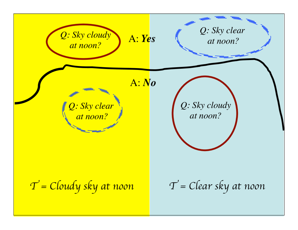
Figure 1: An example of correct prediction as weak inference, where for simplicity determinism is assumed. The set $U$ of all possible histories of the universe is the full rectangle, including both the yellow and blue subsets, which correspond to the two possible states of the sky at noon. Two of the possible questions of the ID are indicated: one of them is asked by the ID in all universes within the union of the two red ellipses, and the other question is asked in all universes within the union of the two blue ellipses. The ID weakly infers $\Gamma$, i.e., correctly predicts the state of the sky at noon, since whichever of the two possible questions it considers, it is guaranteed that its answer is correct.

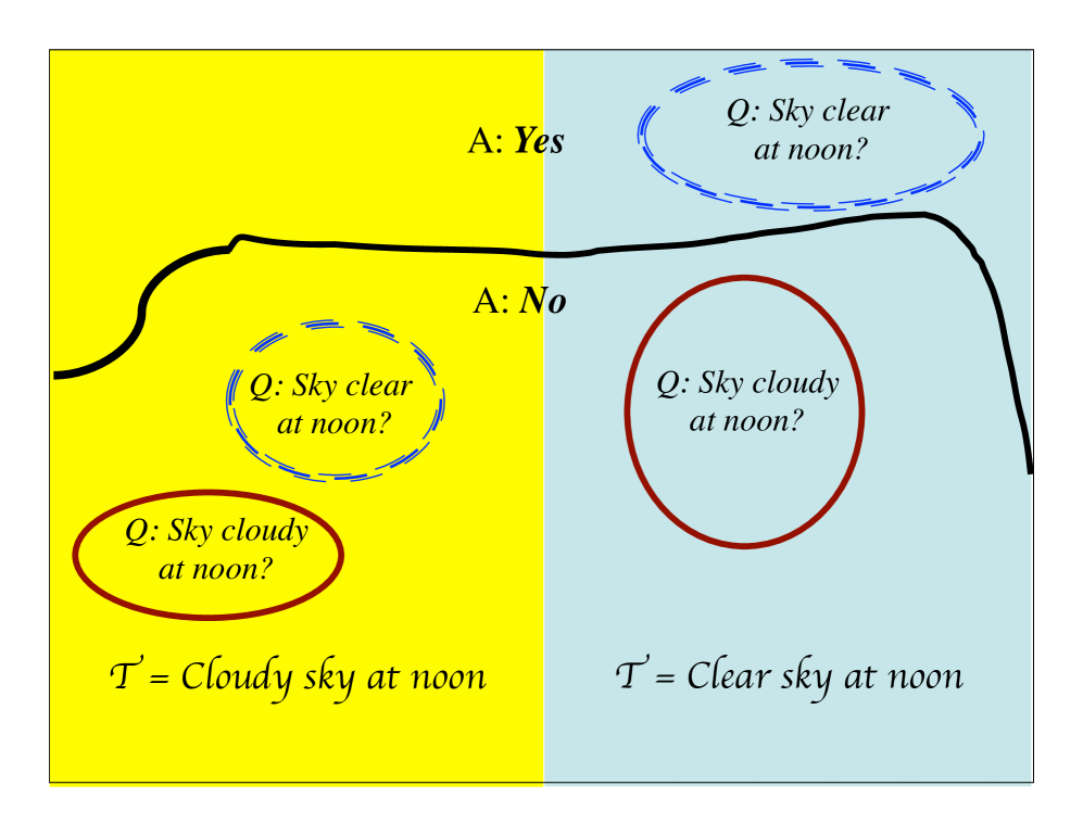
Figure 2: An example where the prediction of an ID of the state of the sky at noon cannot be guaranteed of being correct, i.e., the ID does not weakly infer the function of $u$ giving the state of the sky at noon. The scenario is identical to the one depicted in Fig. 1, except that if the ID is asked the question, “will the sky be cloudy at noon?”, and the sky in fact will be cloudy at noon, the ID will answer ’no’, which is incorrect.

Example 4.

While it is clearly grounded in a real-world scenario, Ex. 2 obscures the mathematical essence of weak inference. A fully abstract, stripped-down example of weak inference is given in the following table, which provides functions $X(u),Y(u)$ and $\Gamma(u)$ for all $u$ in a space $U$. In this minimal example, $U$ has only three elements:

$u$	$X(u)$	$Y(u)$	$\Gamma(u)$
a	1	1	1
b	2	-1	1
c	1	-1	2

In this example, $\Gamma(U)=\{1,2\}$, so we are concerned with two probes, $\delta_{1}$ and $\delta_{2}$. Setting $X(u)=2$ means that $u=b$, which in turn means that $\Gamma(u)=1$ and $Y(u)=-1$. So setting $X(u)=2$ guarantees that $\Gamma(u)\neq 2$, and so $\delta_{2}(\Gamma(u))=Y(u)$ (which in this case equals -1, the answer ’no’). So the setup value $x=2$ ensures that the ID correctly answers the binary question, “does $\Gamma(u)=2$?”, in the negative. Similarly, setting $X(u)=1$ guarantees that $\delta_{1}(\Gamma(u))=Y(u)$, so that it ensures that the ID correctly answers the binary question, “does $\Gamma(u)=1$?”, in the positive.

Ex. 4 shows that weak inference can hold even if $X(u)=x$ doesn’t always fix a unique value for $Y(u)$. Such non-uniqueness is typical when the device is being used for observation. Setting up a device to observe a variable outside of that device restricts the set of possible universes; only those $u$ are allowed that are consistent with the observation device being set up that way to make the desired observation. But typically just setting up an observation device to observe what value a variable has doesn’t uniquely fix the value of that variable.

As discussed in App. B of wolp08b , the definition of weak inference is very unrestrictive. For example, a device ${\mathcal{D}}$ is ‘given credit’ for correctly answering probe $\delta(\Gamma(u))$ if there is any $x\in X(U)$ such that $X(u)=x\Rightarrow Y(u)=\delta({\Gamma(u)})$. In particular, ${\mathcal{D}}$ is given credit even if the binary question we would associate with $x$ (under some particular physical interpretation of what $X$, like in Ex. 1 and Ex. 2) is not whether $\Gamma(u)=\gamma$, but some other question. In essence, the device receives credit even if it gets the right answer by accident.

Unless specified otherwise, a device written as “${{{\mathcal{D}}}}_{i}$” for any integer $i$ is implicitly presumed to have domain $U$, with setup function $X_{i}$ and conclusion function $Y_{i}$ (and similarly for no subscript). Similarly, unless specified otherwise, expressions like “min${}_{x_{i}}$” mean min${}_{x_{i}\in X_{i}(U)}$.

II.4 The two Laplace’s Demon theorems

“An intellect which at a certain moment would know all forces that set nature in motion, and all positions of all items of which nature is composed, if this intellect were also vast enough … nothing would be uncertain and the future just like the past would be present before its eyes.”

— Pierre Simon Laplace, “A Philosophical Essay on Probabilities”

There are limitations on the ability of any device to weakly infer functions. Perhaps the most trivial is the following:

Proposition 1.

For any device ${\mathcal{D}}$, there is a function that ${\mathcal{D}}$ does not infer.

Proof.

Choose $\Gamma$ to be the function $Y$, so that the device is trying to infer itself. Then choose the negation probe $\delta(y\in{\mathbb{B}})=-y$ to see that such inference is impossible. (Also see wolp08b .) ∎

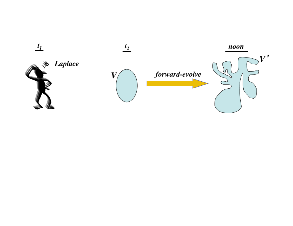
Figure 3: The time $t_{1}$ is less than $t_{2}$, which in turn is less than noon. $V$ is the set of all time-$t_{2}$ universes where Laplace is thinking the answer “yes” in response to the $t_{1}$ question Laplace heard — whatever that question was. $V^{\prime}$ is $V$ evolved forward to noon. At $t_{1}$, we ask Laplace, “will the universe be outside $V^{\prime}$ at noon?” It is impossible for Laplace to answer correctly, no matter what his computational capabilities are, what the laws of the universe are, etc.

It is interesting to consider the implications of Prop. 1 for the case where the inference is prediction, as in Ex. 2. Depending on how precisely one interprets Laplace, Prop. 1 means that he was wrong in his claim about the ability of an “intellect” to make accurate predictions: even if the universe were a giant clock, it could not contain an intellect that could reliably predict the universe’s future state before it occurred. More precisely, for all $\Gamma$ as in Prop. 1, there could be an intellect ${\mathcal{D}}$ that can infer $\Gamma$. However Prop. 1 tells us that for any fixed intellect, there must exist a $\Gamma$ that the intellect cannot infer. (See Fig. 3.) The “intellect” Laplace refers to is commonly called Laplace’s “demon”, so I sometimes refer to Prop. 1 as the “first (Laplace’s) demon theorem”.

One might think that Laplace could circumvent the first demon theorem by simply constructing a second demon, specifically designed to infer the $\Gamma$ that thwarts his first demon. Continuing in this way, one might think that Laplace could construct a set of demons that, among them, could infer any function $\Gamma$. Then he could construct an “overseer demon” that would choose among those demons, based on the function $\Gamma$ that needs to be inferred. However this is not possible. To see this, simply redefine the device ${\mathcal{D}}$ in Prop. 1 to be the combination of Laplace with all of his demons.

These limitations on prediction hold even if the number of possible states of the universe is countable (or even finite), or if the inference device has super-Turning capabilities. It holds even if the current formulation of physics is wrong; it does not rely on chaotic dynamics, physical limitations like the speed of light, or quantum mechanical limitations.

Note as well that in Ex. 2’s model of a prediction system the actual values of the times of the various events are not specified. So in particular the impossibility result of Prop. 1 still applies to that example even if $t_{3}<t_{2}$ — in which case the time when the agent provides the prediction is after the event they are predicting. Moreover, consider the variant of Ex. 2 where the agent programs a computer to do the prediction, as discussed in Footnote 3 in that example. In this variant, the program that is input to the prediction computer could even contain the future value that the agent wants to predict. Prop. 1 would still mean that the conclusion that the agent using the computer comes to after reading the computer’s output cannot be guaranteed to be correct.

Prop. 1 tells us that any inference device ${\mathcal{D}}$ can be “thwarted” by an associated function. However it does not forbid the possibility of some second device that can infer that function that thwarts ${\mathcal{D}}$. To analyze issues of this sort, and more generally to analyze the inference relationships within sets of multiple functions and multiple devices, we start with the following definition:

Definition 3.

Two devices $(X_{1},Y_{1})$ and $(X_{2},Y_{2})$ are (setup) distinguishable iff $\forall x_{1},x_{2},\exists u\in U$ such that $X_{1}(u)=x_{1},X_{2}(u)=x_{2}$.

No device is distinguishable from itself. Distinguishability is symmetric, but non-transitive in general (and obviously not reflexive).

Having two devices be distinguishable means that no matter how the first device is set up, it is always possible to set up the second one in an arbitrary fashion; the setting up of the first device does not preclude any options for setting up the second one. Intuitively, if two devices are not distinguishable, then the setup function of one of the devices is partially “controlled” by the setup function of the other one. In such a situation, they are not two fully separate, independent devices.

I will say that one ID $(X,Y)$ can weakly infer a second one, $(X^{\prime},Y^{\prime})$, if it can weakly infer the conclusion of the second ID, $Y^{\prime}$. (See wolp08b for an example.)

Proposition 2.

No two distinguishable devices $(X,Y)$ and $(X^{\prime},Y^{\prime})$ can weakly infer each other.

I will call Prop. 7 the “second (Laplace’s) demon theorem”. See Fig. 4 for an illustration of Prop. 7, for two IDs called “Bob” and “Alice”, in which they do not directly infer one another’s conclusion, but rather infer functions of those conclusions.

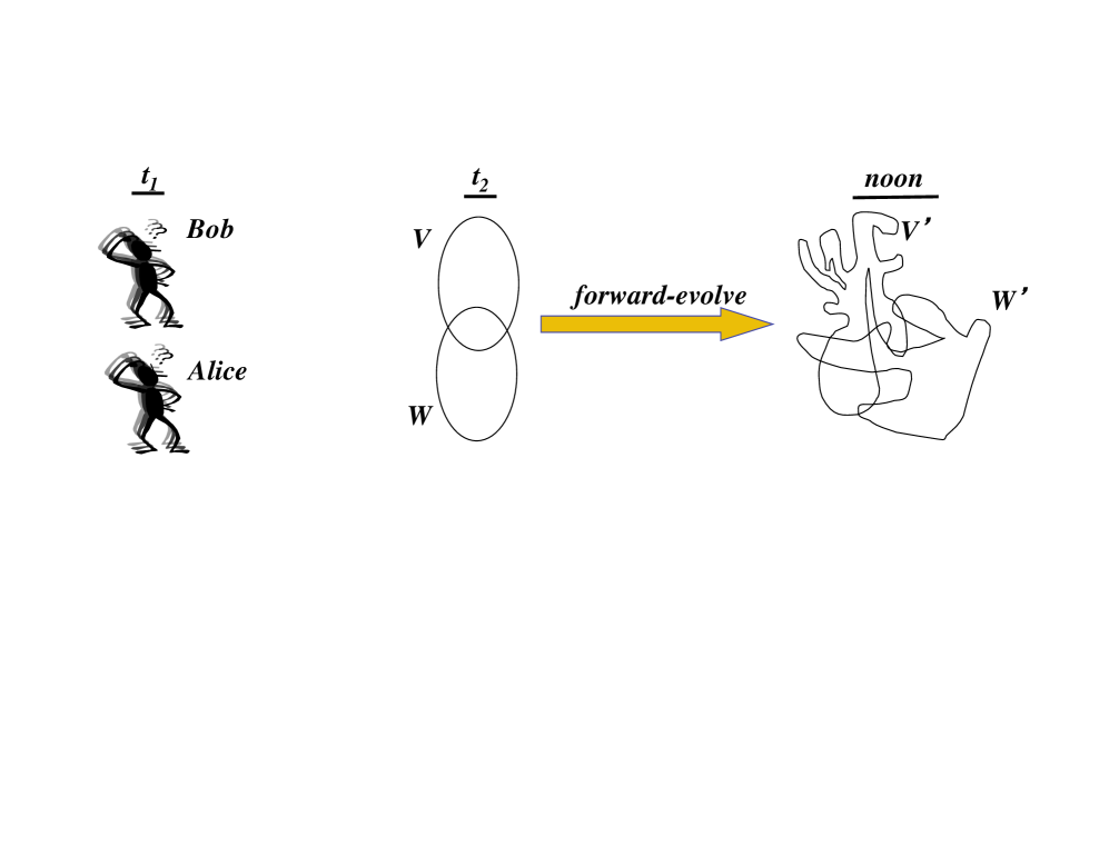
Figure 4: The time $t_{1}$ is less than $t_{2}$, which in turn is less than noon. $V$ is the set of all time-$t_{2}$ universes where Bob is thinking the answer “yes” in response to the $t_{1}$ question Bob heard — whatever that question was. $W$ is the set of all time-$t_{2}$ universes where Alice is thinking the answer “yes” in response to the $t_{1}$ question Alice heard — whatever that question was. $V^{\prime}$ is $V$ evolved forward to noon, and $W^{\prime}$ is $W$ evolved forward to noon. At $t_{1}$, we ask Bob, “will the universe be in $W^{\prime}$ at noon?” (i.e., “is Alice thinking ‘yes’ at $t_{2}$?”). At that time we also ask Alice, “will the universe be outside of $V^{\prime}$ at noon?” (i.e., “is Bob not thinking ‘yes’ at $t_{2}$?”). It is impossible for both Bob and Alice to answer correctly, no matter what their computational capabilities are, what the laws of the universe are, etc.

This second Laplace’s demon theorem establishes that a whole class of functions cannot be inferred by ${\mathcal{D}}$ (namely the conclusion functions of devices that are distinguishable from ${\mathcal{D}}$ and also can infer ${\mathcal{D}}$). More generally, let $\mathcal{S}$ be a set of devices, all of which are distinguishable from one another. Then the second demon theorem says that there can be at most one device in $\mathcal{S}$ that can infer all other devices in $\mathcal{S}$. It is important to note that the distinguishability condition is crucial to the second demon theorem; mutual weak inference can occur between non-distinguishable devices.

In barrow2011godel Barrow speculated whether “only computable patterns are instantiated in physical reality”. There “computable” is defined in the sense of Turing machine theory. However we can also consider the term as meaning “can be evaluated by a real world computer”. If so, then his question is answered — in the negative — by the Laplace demon theorems.

By combining the two demon theorems it is possible to establish the following:

Corollary 3.

Consider a pair of devices ${\mathcal{D}}=(X,Y)$ and ${{{\mathcal{D}}}^{\prime}}=(X^{\prime},Y^{\prime})$ that are distinguishable from one another and whose conclusion functions are inequivalent. Say that ${{{\mathcal{D}}}^{\prime}}$ weakly infers ${\mathcal{D}}$. Then there are at least three inequivalent surjective binary functions $\Gamma$ that ${\mathcal{D}}$ does not infer.

In particular, Coroll. 3 means that if any device in a set of distinguishable devices with inequivalent conclusion functions is sufficiently powerful to infer all the others, then each of those others must fail to infer at least three inequivalent functions.

II.5 Strong inference — inference of entire functions

As considered in computer science theory, a computer is an entire map taking an arbitrary “input” given by the value of a physical variable, $\Gamma_{1}(u)$, to an “output” also given by the value of a physical variable, $\Gamma_{2}(u)$ hopcroft2000jd . It is concerned with saying how the value of $\Gamma_{2}(u)$ would change if the value of $\Gamma_{1}(u)$ changed. So it is concerned with two separate physical variables. In contrast, weak inference is only concerned with inferring the value of a single physical variable, $\Gamma(u)$, not the relationship between two variables.

So we cannot really say that a device “infers a computer” if we only use the weak inference concept analyzed above. In this subsection we extend the theory of inference devices to include inference of entire functions. In addition to allowing us to analyze inference of computers, this lays the groundwork for the analysis in the next section of the relation between inference and algorithmic information theory.

To begin, suppose we have a function $f$ that relates two physical variables. Since those two variables are themselves functions defined over $U$, in general $f$ is not. To be more precise, suppose that there are two function $S$ and $T$ defined over $U$, where $S$ refines $T$, and that for all $s\in S(u)$, $f(s)=T(S^{-1}(s))$ is single-valued. We want to define what it means for a device to be able to “emulate” the entire mapping taking any $s\in S(U)$ to the associated value $f(s)=T(S^{-1}(s))$.

One way to do this is to strengthen the concept of weak inference, so that for any desired input value $s\in S(U)$, the ID in question can simultaneously infer the output value $f(s)$ while also forcing the input to have the value $s$. In other words, for any pair $(s\in S(U),t\in T(U))$, by appropriate choice of $x\in X(U)$ the ID $(X,Y)$ simultaneously answers the probe $\delta_{t}$ correctly (as in the concept of weak inference) and forces $S(u)=s$. In this way, when the ID “answers $\delta_{t}$ correctly”, it is answering whether $f(s)=t$ correctly, for the precise $s$ that it is setting. By being able to do this for all $s\in S(U)$, the ID can emulate the function $f$.

Extending this concept from single-valued functions $f$ to include multivalued functions results in the following definition:

Definition 4.

Let $S$ and $T$ be functions both defined over $U$. A device $(X,Y)$ strongly infers $(S,T)$ iff $\forall\;\delta\in{\mathcal{P}}(T)$ and all $s\in S(U)$, $\exists\;x$ such that $X(u)=x\Rightarrow\{S(u)=s,Y(u)=\delta(T(u))\}$.

If $(X,Y)$ strongly infers $(S,T)$ we write $(X,Y)\gg(S,T)$.

By considering the special case where $T(U)={\mathbb{B}}$, we can use strong inference to formalize what it means for one device to emulate another device:

Definition 5.

A device $(X_{1},Y_{1})$ strongly infers a device $(X_{2},Y_{2})$ iff $\forall\;\delta\in{\mathcal{P}}(Y_{2})$ and all $x_{2}$, $\exists\;x_{1}$ such that $X_{1}=x_{1}\Rightarrow X_{2}=x_{2},Y_{1}=\delta(Y_{2})$.

See App. B in wolp08b for a discussion of how unrestrictive Def. 5 is.

Def. 5 might seem peculiar, since $(X,Y)\gg(S,T)$ means that in a certain sense the function $X$ controls what the input to the function $s\rightarrow T(S^{-1}(S))$ is. However, by a simple change in perspective of what device is doing the strong inference, we can see that Def. 5 applies even to scenarios that (before the change in perspective) do not involve such control. This is illustrated in the following example:

Example 5.

Suppose ${{{\mathcal{D}}}}_{2}$ is a device that (for example) can be used to make predictions about the future state of the weather. Let $\Gamma$ be the set of future weather states that the device can predict, and let $X_{2}$ be the set of possible current meteorological conditions. So if this device can in fact infer the future state of the weather, then for any question $\delta_{\gamma}$ of whether the future weather will have value $\gamma$, there is some current condition $x_{2}$ such that if ${{{\mathcal{D}}}}_{2}$ is set up with that $x_{2}$, it correctly answers whether the associated future state of the weather will be $\gamma$. On the other hand, if ${{{\mathcal{D}}}}_{2}\not>\Gamma$, then there is some such question of the form, “will the future weather be $\gamma$?” such that for no input to the device of the current meteorological conditions will the device necessarily produce an answer $y_{2}$ to the question that is correct.

One way for us to be able to conclude that some device ${{{\mathcal{D}}}}^{\prime}=(X^{\prime},Y^{\prime})$ can “emulate” this behavior of ${{{\mathcal{D}}}}_{2}$ is to set up ${{{\mathcal{D}}}}_{2}$ with an arbitrary value $x_{2}$, and confirm that ${{{\mathcal{D}}}}^{\prime}$ can infer the associated value of $Y_{2}$. So we require that for all $x_{2}$, and all $\delta\in\mathcal{P}(Y_{2})$, $\exists x^{\prime}$ such that if $X_{2}=x_{2}$ and $X^{\prime}=x^{\prime}$, then $Y=\delta(Y_{2})$.

Now define a new device ${{{\mathcal{D}}}}_{1}$, with its setup function defined by $X_{1}(u)=(X^{\prime}(u),X_{2}(u))$ and its conclusion function equal to $Y^{\prime}$. Then our condition for confirming that ${{{\mathcal{D}}}}^{\prime}$ can emulate ${{{\mathcal{D}}}}_{2}$ gets replaced by the condition that for all $x_{2}$, and all $\delta\in\mathcal{P}(Y_{2})$, $\exists x_{1}$ such that if $X_{1}=x_{1}$, then $X_{2}=x_{2}$ and $Y=\delta(Y_{2})$. This is precisely the definition of strong inference.

Say we have a Turing machine (TM) $T_{1}$ that can emulate another TM, $T_{2}$ (e.g., $T_{1}$ could be a universal Turing machine (UTM), able to emulate any other TM). Such “emulation” means that $T_{1}$ can perform any particular calculation that $T_{2}$ can. The analogous relationship holds for IDs, if we translate “emulate” to “strongly infer”, and translate “perform a particular calculation” to “weakly infer”. In addition, like UTM-style emulation (but unlike weak inference), strong inference is transitive. These results are formalized as follows:

Proposition 4.

Let ${{{\mathcal{D}}}}_{1}$, ${{{\mathcal{D}}}}_{2}$ and ${{{\mathcal{D}}}}_{3}$ be a set of inference devices over $U$ and $\Gamma$ a function over $U$. Then:

i) ${{{\mathcal{D}}}}_{1}\gg{{{\mathcal{D}}}}_{2}$ and ${{{\mathcal{D}}}}_{2}>\Gamma$ $\Rightarrow$ ${{{\mathcal{D}}}}_{1}>\Gamma$.

ii) ${{{\mathcal{D}}}}_{1}\gg{{{\mathcal{D}}}}_{2}$ and ${{{\mathcal{D}}}}_{2}\gg{{{\mathcal{D}}}}_{3}$ $\Rightarrow$ ${{{\mathcal{D}}}}_{1}\gg{{{\mathcal{D}}}}_{3}$.

In addition, strong inference implies weak inference, i.e., ${{{\mathcal{D}}}}_{1}\gg{{{\mathcal{D}}}}_{2}\Rightarrow{{{\mathcal{D}}}}_{1}>{{{\mathcal{D}}}}_{2}$.

Most of the properties of weak inference have analogs for strong inference:

Proposition 5.

Let ${{{\mathcal{D}}}}_{1}$ be a device over $U$.

i) There is a device ${{{\mathcal{D}}}}_{2}$ such that ${{{\mathcal{D}}}}_{1}\not\gg{{{\mathcal{D}}}}_{2}$.

ii) Say that $\forall\;x_{1}$, $|X_{1}^{-1}(x_{1})|>2$. Then there is a device ${{{\mathcal{D}}}}_{2}$ such that ${{{\mathcal{D}}}}_{2}\gg{{{\mathcal{D}}}}_{1}$.

Strong inference also obeys a restriction that is analogous to Prop. 2, except that there is no requirement of setup-distinguishability:

Proposition 6.

No two devices can strongly infer each other.

Recall that there are entire functions that are not computable by any TM, in the sense that no TM can correctly compute the value of that function for every input to that function. On the other hand, trivially, any single output value of a function can be computed by some TM (just choose the TM that prints that value and then halts). The analogous distinction holds for inference devices:

Proposition 7.

Let $U$ be any countable space with at least two elements.

1. For any function $\Gamma$ over $U$ such that $|\Gamma(U)|\geq 3$ there is a device ${\mathcal{D}}$ that weakly infers $\Gamma$;

2. There is a (vector-valued) function $(S,T)$ over $U$ that is not strongly inferred by any device.

Proof.

The proof is by construction. Let $X(u)$ be the identity function (so that each $u\in U$ has its own, unique value $x$). Choose $Y(u)$ to equal $1$ for exactly one $u$, $\bar{u}$. Then whatever the value $\gamma:=\Gamma(\bar{u})\in\Gamma(U)$ happens to be, for the probe $\delta_{\gamma}$ we can choose $x=X(\bar{u})$, so that the device correctly answers ‘yes’ to the question of whether $\Gamma(u)=\Gamma(\bar{u})$. For any other probe $\delta_{\gamma^{\prime}}$, note that since $|\Gamma(U)|\geq 3$, there must be a $u^{\prime}\in U$ such that $\Gamma(u^{\prime})\neq\gamma^{\prime}$. Moreover, by construction $Y(u^{\prime})=-1$. So if we choose $x$ to be $X(u^{\prime})$, then the device correctly answers ‘no’ to the question of whether $\Gamma(u^{\prime})=\gamma^{\prime}$. Since this is true for any $\gamma^{\prime}\neq\Gamma(\bar{u})$, this completes a proof of the first claim.

We also prove the second claim by construction. Choose both $S$ and $T$ to be the identity function, i.e., $S(u)=u$ and $T(u)=u$ for all $u$, so that $|S(U)|=|T(U)|=|U|$. So by the first requirement for some device $(X,Y)$ to strongly infer $(S,T)$, it must be that for any $s$, there is a value of $X$, $x(s)$, such that $X(u)=x(s)\Rightarrow S(u)=s$. Since $S$ is a bijection, this means that $x(s)$ must be a single-valued function, for each $s$ choosing a unique ($x$ which in turn chooses a unique) $u$. Since $T$ is also a bijection, this means that $Y(X^{-1}(x(s))$ must equal $1$, in order for the device to correctly answer ‘yes’ to the probe of whether $T(u)=\delta_{T(S^{-1}(s))}$. However since this is true for all $s\in S(U)$, it is true for all $u\in U$. So $Y(U)$ is a singleton, contradicting the requirement that the conclusion function of any device be binary-valued. ∎

III Inference in stochastic universes

III.1 Stochastic inference

There are several ways to extend the analysis above to incorporate a probability measure $P$ over $U$, so that inference is not exact, but only holds under some probability. In this subsection we present some of the elementary properties of one such measure of stochastic inference.

Once there is a distribution over $U$, all functions like $X$, $Y$ and $\Gamma$ become random variables. Now recall that $\delta_{\gamma}(\Gamma)$ is shorthand for the function $u\in U\rightarrow\delta_{\gamma}(\Gamma(u))$ — and so now it is a random variable. Bearing this in mind, the measure of stochastic inference we will consider here is defined as follows:

Definition 6.

Let $P(u\in U)$ be a probability measure and $\Gamma$ a function with domain $U$ and finite range. Then we say that a device $(X,Y)$ (weakly) infers $\Gamma$ with (covariance) accuracy

$$cov({\mathcal{D}},\Gamma) := \frac{\sum_{\delta\in{\mathcal{P}}(\Gamma)}\max_{x}\big{[}{\mathbb{E}}_{P}(Y\delta(\Gamma)\mid x)\big{]}}{|\Gamma(U)|}$$

Writing it out explicitly, for countable $U$, the numerator in Def. 6 is

$$\sum_{\gamma\in\Gamma(U)}\max_{x\in X(U)}\bigg{[}\sum_{u}Y(u)\delta_{\gamma}(\Gamma(u))P(u\mid x)\bigg{]}$$ (4)

Intuitively, this is a probe-averaged, best-case (over $x\in X(U)$) probability of answering the probe correctly.

Covariance accuracy is a way to quantify the degree to which ${\mathcal{D}}>\Gamma$ when the inference is subject to uncertainty. Clearly, $cov({\mathcal{D}},\Gamma)\leq 1.0$, and if $P$ is nowhere 0, then $cov({\mathcal{D}},\Gamma)=1.0$ iff ${\mathcal{D}}>\Gamma$. Covariance accuracy obeys the following bound:

Proposition 8.

Let $P$ be a probability measure over $U$, ${\mathcal{D}}=(X,Y)$ a device, and $\Gamma$ a function over $U$ with finite $|\Gamma(U)|$. Then

$$cov({\mathcal{D}},\Gamma)\geq\frac{(2-|\Gamma(U)|)\max_{x}\big{[}{\mathbb{E}}_{P}(Y\mid x)\big{]}}{|\Gamma(U)|}$$

Proof.

For any probe $\delta_{\gamma}$ of $\gamma\in\Gamma(U)$, let $M_{\gamma}=\max_{x}\big{[}{\mathbb{E}}_{P}(Y\delta_{\gamma}(\Gamma)\mid x)\big{]}$. Define $x_{m}:=\rm{argmax}_{x}\big{[}{\mathbb{E}}_{P}(Y\mid x)\big{]}$. Then $M_{\gamma}\geq{\mathbb{E}}_{P}(Y\delta_{\gamma}(\Gamma)\mid x_{m})$ and

$$\begin{split}cov({\mathcal{D}},\Gamma)&=\frac{\sum_{\gamma\in\Gamma(U)}M_{\gamma}}{|\Gamma(U)|}\geq\frac{\sum_{\gamma\in\Gamma(U)}{\mathbb{E}}_{P}(Y\delta_{\gamma}(\Gamma)\mid x_{m})}{|\Gamma(U)|}\\ &=\frac{\sum_{u}P(u\mid x_{m})\sum_{\gamma}Y(u)\delta_{\gamma}(\Gamma(u))}{|\Gamma(U)|}\\ &=\frac{\sum_{u}P(u\mid x_{m})(2-|\Gamma(U)|)Y(u)}{|\Gamma(U)|}\\ &=\frac{(2-|\Gamma(U)|){\mathbb{E}}_{P}(Y\mid x_{m})}{|\Gamma(U)|}\\ &=\frac{(2-|\Gamma(U)|)\max_{x}\big{[}{\mathbb{E}}_{P}(Y\mid x)\big{]}}{|\Gamma(U)|}.\end{split}$$

∎

This bound is sharp, as can be seen from the following example.

Example 6.

Fix some device ${\mathcal{D}}$ and a value $|\Gamma(U)|<\infty$. Next divide each cell of the partition $X\times Y$ into $|\Gamma(U)|$ parts and assign them equal probability. Also map those cells to 1, $\dotso,|\Gamma(U)|$, so that $\Gamma(U)=\{1,\dotso,|\Gamma(U)|\}.$ For any given $x\in X$, let $a_{x}=P(Y=1\mid x),b_{x}=P(Y=-1\mid x)$. For any $x\in X(U),\gamma\in\Gamma(U)$ and associated probe $\delta_{\gamma}$,

$$\begin{split}\mathbb{E}_{P}(Y\delta_{\gamma}(\Gamma)\mid x)&=\frac{a_{x}+(|\Gamma(U)|-1)b_{x}-(|\Gamma(U)|-1)a_{x}+b_{x}}{|\Gamma(U)|}\\ &=\frac{(2-|\Gamma(U)|)(a_{x}-b_{x})}{|\Gamma(U)|}=\frac{(2-|\Gamma(U)|){\mathbb{E}}_{P}(Y\mid x)}{|\Gamma(U)|}.\end{split}$$

We can use this to evaluate

$$\begin{split}M_{\gamma}&:=\max_{x}\big{[}{\mathbb{E}}_{P}(Y\delta_{\gamma}(\Gamma)\mid x)\big{]}\\ &=\frac{(2-|\Gamma(U)|)\;\max_{x}\big{[}{\mathbb{E}}_{P}(Y\mid x)\big{]}}{|\Gamma(U)|}\end{split}$$

Since this is the same for all probe parameter values $\gamma$,

$$cov({\mathcal{D}},\Gamma)=\frac{(2-|\Gamma(U)|)\;\max_{x}\big{[}{\mathbb{E}}_{P}(Y\mid x)\big{]}}{|\Gamma(U)|}$$

which establishes the claim.

The term $\frac{2-|\Gamma(U)|}{|\Gamma(U)|}$ in Prop. 8 depends only on the size of the space $\Gamma(U)$. The other term, max${}_{x}\big{(}{\mathbb{E}}_{P}(Y\mid x)\big{)}$, can be viewed as a measure of the “inference power” of the device, by analogy with the power of a statistical test. It quantifies the device’s ability to say ‘yes’.

In the previous section some a priori restrictions on the capabilities of IDs were presented. These restrictions involved whether certain properties of IDs can(not) be guaranteed with complete certainty. When we have a probability distribution over $U$ it is appropriate to replace consideration of “guaranteed” properties with consideration of properties that are likely but not necessarily guaranteed, e.g., as quantified with covariance accuracy. When we do that the restrictions of the previous section get modified, sometimes quite substantially. This is illustrated in the next two propositions.

First, by Prop. 4(i), if for devices ${\mathcal{D}}_{1}$, ${\mathcal{D}}_{2}$ and function $\Gamma$, ${\mathcal{D}}_{1}\gg{\mathcal{D}}_{2}$ and ${\mathcal{D}}_{2}>\Gamma$, then ${\mathcal{D}}_{1}>\Gamma$. In covariance terms, this says that if ${\mathcal{D}}_{1}\gg{\mathcal{D}}_{2}$ and $cov({\mathcal{D}}_{2},\Gamma)=1.0$, then $cov({\mathcal{D}}_{1},\Gamma)=1.0$. What happens to $cov({\mathcal{D}}_{1},\Gamma)$ if $cov({\mathcal{D}}_{2},\Gamma)<1.0$? A partial answer is given by the following result:

Proposition 9.

There are devices ${\mathcal{D}}$, ${\mathcal{D}}^{\prime}$, probability distribution $P$ defined over $U$, and function $\Gamma$, such that ${\mathcal{D}}^{\prime}\gg{\mathcal{D}}$ and $cov({\mathcal{D}},\Gamma)$ is arbitrarily close to 1.0 while $cov({\mathcal{D}}^{\prime},\Gamma)$ = 0.

Proof.

The proof is by example.

Let $U$ have ten states, labeled A$,\ldots,$ J and suppose that the functions $P,\Gamma,{\mathcal{D}}=(X,Y)$ and ${\mathcal{D}}^{\prime}=(X^{\prime},Y^{\prime})$ are as in Fig. 5, with $0\leq p\leq 1$.

Figure 5: Specification of a scenario in which the stochastic version of Prop. 4(i), concerning “transitivity” of weak inference through strong inference, fails drastically.

1. To verify that ${\mathcal{D}}^{\prime}\gg{\mathcal{D}}$, for the $1$-probe, for $x=1,2$, choose $x^{\prime}=1,3$, respectively. For the $-1$-probe, for $x=1,2$, choose $x^{\prime}=2,4$, respectively.

2. $cov({\mathcal{D}},\Gamma)=p$. To see this, for the $1$-probe, evaluate $\max_{x}{\mathbb{E}}_{P}(Y\delta_{1}(\Gamma)\mid x)=p$, the maximum occurring for $x=1$. Similarly, for the $-1$-probe, evaluate $\max_{x}{\mathbb{E}}_{P}(Y\delta_{-1}(\Gamma)\mid x)=p$, the maximum occurring for $x=2$.

3. $cov({\mathcal{D}}^{\prime},\Gamma)=0$. To see this for both probes, note that ${\mathbb{E}}_{P}(Y^{\prime}\delta(\Gamma)\mid x^{\prime})=0$ for each $x^{\prime}$.

The proof is completed by taking $p\rightarrow 1$. ∎

To understand Prop. 9, recall that the definition of ${\mathcal{D}}^{\prime}\gg{\mathcal{D}}$ requires that for any $x\in X(U)$ and for any probe $\delta_{\gamma}\in{\mathcal{P}}(\Gamma)$, there be some $x^{\prime}$ and associated $X^{\prime-1}(x^{\prime})\subseteq U$ for which ${\mathcal{D}}^{\prime}$ successfully emulates ${\mathcal{D}}$’s behavior at inferring $\delta_{\gamma}$. If the inference ${\mathcal{D}}>\Gamma$ is perfect, then ${\mathcal{D}}^{\prime}$ also infers $\Gamma$. However, if the inference ${\mathcal{D}}>\Gamma$ is only partially correct, then that value $x^{\prime}$ and associated subset of $U$, under which ${\mathcal{D}}^{\prime}\gg{\mathcal{D}}$ may be precisely those $u$ for which ${\mathcal{D}}$ performs badly at inferring $\delta_{\gamma}$. Thus, ${\mathcal{D}}$ may do an excellent, though imperfect, job overall of inferring $\Gamma$ while ${\mathcal{D}}^{\prime}$ fails completely.

The second example of how the restrictions of the previous section get modified by introducing a probability distribution is that this makes the second Laplace’s impossibility theorem become “barely true”:

Proposition 10.

There are devices ${\mathcal{D}}$ and ${\mathcal{D}}^{\prime}$ with $X$ and $X^{\prime}$ setup-distinguishable and a distribution $P$ where both $cov({\mathcal{D}},{\mathcal{D}}^{\prime})$ and $cov({\mathcal{D}}^{\prime},{\mathcal{D}})$ are arbitrarily close to 1.

Proof.

The proof is by example.

Let $U$ have sixteen states, labeled A, $\ldots$, P and suppose that the functions $P,\Gamma,{\mathcal{D}}=(X,Y)$ and ${\mathcal{D}}^{\prime}=(X^{\prime},Y^{\prime})$ are as in Fig. 6, with arbitrary $0<b<1/6$, and $a=(1-6b)/2$.

By inspection, $X$ and $X^{\prime}$ are setup distinguishable. Next, plugging in yields $cov({\mathcal{D}},{\mathcal{D}}^{\prime})=cov({\mathcal{D}},Y^{\prime})=a/(a+b)$. Moreover $cov({\mathcal{D}}^{\prime},{\mathcal{D}})=cov({\mathcal{D}},{\mathcal{D}}^{\prime})$ by symmetry of the columns in Fig. 6. (${\mathbb{E}}_{P}(YY^{\prime}\mid X=1)=(a-b)/(a+b)$ and ${\mathbb{E}}_{P}(YY^{\prime}\mid X=-1)=-1$.)

Figure 6: Specification of a scenario in which the stochastic version of Prop. 2, concerning simultaneous inference of two setup-distinguishable IDs, fails drastically.

So by taking $b$ arbitrarily close to 0, both of the covariances can be made arbitrarily close to 1. ∎

Prop. 10 shows that in a certain sense, as soon as any stochasticity is introduced into the universe, having two devices be setup-distinguishable no longer restricts their ability to simultaneously infer each other. However if we replace setup-distinguishability with the property that the setup functions of the two devices are statistically independent, then we recover strong restrictions on simultaneous inference.

To illustrate this, let $M$ be the four-dimensional hypercube $\{0,1\}^{4}$. Define the following three functions over $\vec{z}\in M$:

1. $k({\vec{z}})=z_{1}+z_{4}-z_{2}-z_{3}$;

2. $m({\vec{z}})=(z_{2}-z_{4})$;

3. $n({\vec{z}})=(z_{3}-z_{4})$.

Proposition 11.

Let $P$ be a probability measure over $U$, and ${{{\mathcal{D}}}}_{1}$ and ${{{\mathcal{D}}}}_{2}$ two devices where $X_{1}(U)=X_{2}(U)={\mathbb{B}}$, and those variables are statistically independent under $P$. Define $P(X_{1}=-1)\equiv\alpha$ and $P(X_{2}=-1)\equiv\beta$. Say that ${{{\mathcal{D}}}}_{1}$ infers ${{{\mathcal{D}}}}_{2}$ with accuracy $\epsilon_{1}$, while ${{{\mathcal{D}}}}_{2}$ infers ${{{\mathcal{D}}}}_{2}$ with accuracy $\epsilon_{2}$. Then

$$\epsilon_{1}\epsilon_{2}\; \leq \;{\mbox{max}}_{{\vec{z}}\in M}\big{|}\alpha\beta[k({\vec{z}})]^{2}+\alpha k({\vec{z}})m({\vec{z}})+\beta k({\vec{z}})n({\vec{z}})+m({\vec{z}})n({\vec{z}})\big{|}.$$

In particular, if $\alpha=\beta=1/2$, then

$$\epsilon_{1}\epsilon_{2}\; \leq \;\frac{{\mbox{max}}_{{\vec{z}}\in M}\;|\;(z_{1}-z_{4})^{2}-(z_{2}-z_{3})^{2}\;|}{4}$$

$$= \;1/4.$$

The maximum for $\alpha=\beta=1/2$ can occur in several ways. One is when $z_{1}=1$, and $z_{2},z_{3},z_{4}$ all equal $0$. At these values, both devices have an inference accuracy of 1/2 at inferring each other. Each device achieves that accuracy by perfectly inferring one probe of the other device, while performing randomly for the remaining probe.

The ID framework as developed to date has no function measuring distance, nor one measuring time. So at present, one cannot even formulate an ID-analog of Heisenberg’s uncertainty principle, never mind try to derive it. It is intriguing that despite this, Prop. 11 is a bound on the product of uncertainties, exactly like Heisenberg’s uncertainty principle. This suggests it may be worth exploring extensions of the ID framework that do involve distance and time, to see what a priori constraints there might be on the product of uncertainties of two IDs that are measuring different aspects of the same system. (This idea is returned to in the last section below.)

Finally, it should be noted that there are other ways to quantify the degree of weak inference when there is intrinsic uncertainty, in addition to covariance accuracy. For example, we could change Def. 6 by replacing the sum over all probes $\delta$ and associated division by $|\Gamma(U)|$ with a minimum over all probes $\delta$. (This amounts to replacing an average-best-case expression with a worst-case expression.)

III.2 The complexity of inference

Constraints on what can be computed by a physical device can be derived from the laws of physics lloyd2000ultimate . There have also been attempts to go the other way, and derive constraints on the laws of physics from computation theory, in particular from algorithmic information theory (AIT) livi08 ; chaitin2004algorithmic ; zure89a ; zure89b ; zurek1990complexity ; zenil2012computable . These often implicitly involve uncertainty about the state of the universe. For example, the use of Kolmogorov complexity to model physical reality is often intimately related to the use of algorithmic probability livi08 ; schmidhuber2000algorithmic ; zuse1969rechnender . (Indeed, the very first line in schmidhuber2000algorithmic is “The probability distribution $P$ from which the history of our universe is sampled represents a theory of everything”.) One way to justify consideration of such a probability distribution in the first place is to identify it with uncertainty of some agent (e.g., a scientist) concerning the state of the universe.

This importance of an agent in attempts to analyze physics using AIT suggests we extend the inference device framework to include structures similar to those considered in AIT. There are several ways to extend the ID framework this way. In this subsection I sketch the starting point for one of them.

Given a TM $T$, the Kolmogorov complexity of an output string $s$ is defined as the size of the smallest input string $s^{\prime}$ that when input to $T$ produces $s$ as output. To construct our inference device analog of this, we need to define the “size” of an input region of an inference device ${\mathcal{D}}$. To do this, we assume we are given a measure $d\mu$ over $U$, and for simplicity restrict attention to functions $\Gamma$ over $U$ with countable range. Then we define the size of $\gamma\in\Gamma(U)$ as -ln$\big{[}\int_{\Gamma^{-1}(\gamma)}d\mu(u)\;1\big{]}$, i.e., the negative logarithm of the measure of all $u\in U$ such that $\Gamma(u)=\gamma$. We write this size as ${\mathcal{M}}_{\mu;\Gamma}(\gamma)$, or just ${\mathcal{M}}(\gamma)$ for short.

We define inference complexity in terms of such a size function using the shorthand introduced just below Eq. (2):

Definition 7.

Let ${\mathcal{D}}$ be a device and $\Gamma$ a function over $U$ where $X(U)$ and $\Gamma(U)$ are countable and ${\mathcal{D}}>\Gamma$. The inference complexity of $\Gamma$ with respect to ${\mathcal{D}}$ and measure $\mu$ is defined as

$${\mathcal{C}}_{\mu}(\Gamma;{\mathcal{D}})\;\; \triangleq \;\;\sum_{\delta\in{\mathcal{P}}(\Gamma)}{\mbox{min}}_{x:X=x\Rightarrow Y=\delta(\Gamma)}[{\mathcal{M}}_{\mu,X}(x)].$$

In the sequel I will often have the measure implicit, and (for example) simply write ${\mathcal{C}}$ rather than ${\mathcal{C}}_{\mu}$. I will also mostly restrict attention to the case where $\mu$ is either a distribution or a semi-measure.

As an example, for the case where inference models the process of prediction, $\Gamma$ corresponds to a potential future state of some system $S$ external to ${\mathcal{D}}$. In this case ${\mathcal{C}}(\Gamma;{\mathcal{D}})$ is a measure of how difficult it currently is for ${\mathcal{D}}$ to predict that future state of $S$. Loosely speaking, the more sensitively that future state depends on current conditions, the greater the inference complexity of predicting that future state.

Inference complexity of any function $\Gamma$ with respect to a device $(X,Y)$ is bounded by the Shannon entropy of $\mu(X)$:

Proposition 12.

For any ID ${\mathcal{D}}$, probability distribution $\mu$, and function $\Gamma$ with a countable image such that ${\mathcal{D}}>\Gamma$,

$${\mathcal{C}}_{\mu}(\Gamma;{\mathcal{D}})\leq|\Gamma|\times H_{\mu}(X)$$

where $H_{\mu}(X)$ is the Shannon entropy of $\mu(X)$.

Proof.

Expand

$$\sum_{\delta\in\mathcal{P}(\Gamma)}\min_{x:X=x\Rightarrow Y=f(\Gamma)}[{\mathcal{M}}_{\mu,X}(x)] \leq \sum_{x\in X(U)}{\mathcal{M}}_{\mu,X}(x)$$

$$\leq -|\Gamma|\sum_{x\in X(U)}\frac{{\mbox{log}}_{2}\mu(x)}{|\Gamma|}$$

$$\leq |\Gamma|H_{\mu}(X)$$

∎

Kolmogorov complexity concerns TMs computing a single output, rather than TMs emulating an entire function from inputs to outputs. The field of algorithmic information theory then analyzes the relation between Kolmogorov complexity and UTMs, i.e., TMs that emulate entire functions from inputs to outputs. Analogously, inference complexity concerns inferring a single value of a variable, i.e., it is defined in terms of weak inference. So to investigate the inference device analog of algorithmic information theory means investigating the relation between inference complexity and IDs that emulate entire functions — which involves strong inference instead of weak inference.

To begin, recall perhaps the most fundamental result in AIT, the invariance theorem. This theorem gives an upper bound on the difference between the Kolmogorov complexity of a string using a particular UTM $T_{1}$ and its complexity if using a different UTM, $T_{2}$. This bound is independent of the computation to be performed, and can be viewed as the Kolmogorov complexity of $T_{1}$ emulating $T_{2}$. Similarly, we can bound how much greater the inference complexity of a function can be for a device ${\mathcal{D}}_{1}$ than it is for a different device ${\mathcal{D}}_{2}$ if ${\mathcal{D}}_{1}$ can strongly infer ${\mathcal{D}}_{2}$:

Proposition 13.

Let ${\mathcal{D}}_{1}$ and ${\mathcal{D}}_{2}$ be two devices and $\Gamma$ a function over $U$ where $\Gamma(U)$ is finite, ${\mathcal{D}}_{1}\gg{\mathcal{D}}_{2}$, and ${\mathcal{D}}_{2}>\Gamma$. Then for any distribution $\mu$,

$${\mathcal{C}}_{\mu}(\Gamma;{\mathcal{D}}_{1})-{\mathcal{C}}_{\mu}(\Gamma;{\mathcal{D}}_{2})\;\;\leq\;\;|\Gamma(U)|\;\times$$

$$\qquad\qquad{\max}_{x_{2}}\bigg{(}\min_{x_{1}:\{X_{1}=x_{1}\Rightarrow X_{2}=x_{2},Y_{1}=Y_{2}\}}[{\mathcal{M}}_{\mu,X_{1}}(x_{1})-{\mathcal{M}}_{\mu,X_{2}}(x_{2})]\bigg{)}.$$

Note that since ${\mathcal{M}}_{\mu,X_{1}}(x_{1})-{\mathcal{M}}_{\mu,X_{2}}(x_{2})={\mbox{ln}}\bigg{[}\frac{\mu(X_{2}^{-1}(x_{2}))}{\mu(X_{1}^{-1}(x_{1}))}\bigg{]}$, the bound in Prop. 13 is independent of the units with which one measures volume in $U$. (Cf. footnote  11.) Furthermore, it is always true that $X_{1}=x_{1}\Rightarrow X_{2}=x_{2},Y_{1}=Y_{2}$ iff $X_{1}^{-1}(x_{1})\subseteq X_{2}^{-1}(x_{2})\;\cap\;(Y_{1}Y_{2})^{-1}(1)$. Accordingly, for all $(x_{1},x_{2})$ pairs arising in the bound in Prop. 13, $\frac{\mu(X_{2}^{-1}(x_{2}))}{\mu(X_{1}^{-1}(x_{1}))}\geq 1$. So the upper bound in Prop. 13 is always non-negative.

The max-min expression on the RHS of Prop. 13 is independent of $\Gamma$. So the bound in Prop. 13 is independent of all aspects of $\Gamma$ except the cardinality of $\Gamma(U)$. Intuitively, the bound is $|\Gamma(U)|$ times the worst-case amount of “computational work” that ${\mathcal{D}}_{1}$ has to do to “emulate” ${\mathcal{D}}_{2}$’s behavior for some particular value of $x_{2}$.

Suppose that it takes a lot of computational work for ${\mathcal{D}}_{2}$ to infer $\Gamma$, and so it also takes a lot of computational work for ${\mathcal{D}}_{1}$ to infer $\Gamma$ by emulating ${\mathcal{D}}_{2}$. However, it might take very little work for ${\mathcal{D}}_{1}$ to infer $\Gamma$ directly. In fact, it may even be that ${\mathcal{C}}(\Gamma;{\mathcal{D}}_{1})<{\mathcal{C}}(\Gamma;{\mathcal{D}}_{2})$:

Proposition 14.

There are devices ${\mathcal{D}}$, ${\mathcal{D}}^{\prime}$, probability distribution $P$ defined over $U$, and function $\Gamma$, such that ${\mathcal{D}}>\Gamma$, ${\mathcal{D}}^{\prime}\gg{\mathcal{D}}$, and ${\mathcal{C}}_{P}(\Gamma;{\mathcal{D}})$ is arbitrarily large, while ${\mathcal{C}}_{P}(\Gamma;{\mathcal{D}}^{\prime})$ is arbitrarily close to the minimum value of $\big{|}\Gamma\big{|}\times\ln(|\Gamma(U)|)$.

Proof.

The proof is by example.

Let $U$ have twelve states, labeled A$,\ldots,$ L and suppose that the functions $P,\Gamma,{\mathcal{D}}^{\prime}=(X,Y)$ and ${\mathcal{D}}=(X,Y)$ are as in Fig. 7, with $1/4<p<1$.

Figure 7: Scenario illustrating discrepancies of complexities of two IDs where one strongly infers the other.

1. To verify that ${\mathcal{D}}>\Gamma$, for the $1$-probe, choose $x=1$. For the $-1$ probe, choose $x=2$.

2. To verify that ${\mathcal{D}}^{\prime}\gg{\mathcal{D}}$, first, for the $1$-probe, for $x=1,2,3$, choose $x^{\prime}=1,3,5$, respecitively. Then for the $-1$-probe, for $x=1,2,3$, choose $x^{\prime}=2,4,6$, respectively.

3. To verify that ${\mathcal{C}}(\Gamma;{\mathcal{D}})$ can be arbitrarily large, first expand it as $-2\ln((1-p)/2)=2\ln(2)-2\ln(1-p)$. (For the 1-probe, $x=1$ and ${\mathcal{M}}_{P,X}(x)=-\ln((1-p)/2)$ and similarly for the -1-probe and $x=2$.)

4. To verify that ${\mathcal{C}}(\Gamma;{\mathcal{D}}^{\prime})$ can be arbitrarily close to its minimal value, write it as $-2\ln(p/2)=2\ln(2)-2\ln(p)$. (For the 1-probe, $x^{\prime}=5$ and ${\mathcal{M}}_{P,X}(x)=-\ln(p/2)$ and similarly for the -1-probe and $x^{\prime}=6$.)

Finally, by taking $p$ arbitrarily close to 1, ${\mathcal{C}}(\Gamma;{\mathcal{D}})$ becomes arbitrarily large while ${\mathcal{C}}(\Gamma;{\mathcal{D}}^{\prime})$ becomes arbitrarily close to the minimum of $2\ln(2)$. ∎

Although there is not space to analyze them here, it is worth noting that there are several ways to translate some of the mathematical structures of algorithmic information theory into the inference device framework. For example, just as a given Turing machine may fail to produce an output for some specific input, so an inference device may fail to reach a conclusion for some specific setup. This motivates the following definition:

Definition 8.

A device $(X,Y)$ halts for setup value $x$ iff $X=x\Rightarrow Y=y$ for some single value $y$.

We say that $x$ is a “halting setup” if $(X,Y)$ halts for $x$. Parelleling the usual definitions in TM theory, we say that an ID is total, or recursive iff it halts for all $x\in X(U)$. So an ID $(X,Y)$ is recursive iff $X$ refines $Y$.

Given this definition of what it means for a device to halt on a given input, we can define the inference analog of a prefix-free Turing machine livi08 :

Definition 9.

Given a semi-measure $\mu$, a device $(X,Y)$ is prefix(-free) iff

$$\sum_{x:{\mathcal{D}}\;halts\;on\;x}2^{-{\mathcal{M}}_{\mu,X}(x)} \leq 1$$

By Kraft’s inequality, if ${\mathcal{D}}$ is prefix-free for a semi-measure $\mu$, then there is a prefix-free code for the set of all halting $x\in X(U)$. Therefore we can identify that set of $x$’s with semi-infinite bit strings, or equivalently with the natural numbers livi08 .

As a final example, note that the min over $x$’s in Def. 7 is a direct analog of the min in the definition of Kolmogorov complexity (there the min is over those strings that when input to a particular UTM result in the desired output string). A natural modification to Def. 7 is to remove the min by considering all $x$’s that cause $Y=\delta(\Gamma)$, not just of one of them:

$${\hat{{\mathcal{C}}}}(\Gamma;{\mathcal{D}})\;\; \triangleq \;\;\sum_{\delta\in{\mathcal{P}}(\Gamma)}-{\mbox{ln}}\left[\;\mu\left(\cup_{x:X=x\Rightarrow Y=\delta(\Gamma)}X^{-1}(x)\right)\;\right]$$

$$= \sum_{\delta\in{\mathcal{P}}(\Gamma)}-{\mbox{ln}}\left[\sum_{x:X=x\Rightarrow Y=\delta(\Gamma)}e^{-{\mathcal{M}}(x)}\right],$$

where the equality follows from the fact that for any $x,x^{\prime}\neq x$, $X^{-1}(x)\cap X^{-1}(x^{\prime})=\varnothing$. The argument of the $\ln(.)$ in this modified version of inference complexity has a direct analog in TM theory: The sum, over all input strings $s$ to a UTM that generates a desired output string $s^{\prime}$, of $2^{-n(s)}$, where $n(s)$ is the bit size of $s$. This is sometimes known as the “algorithmic” or “Solomonoff” probability of $s^{\prime}$ livi08 in the theory of TMs.

IV Modeling the physical universe in terms of inference devices

I now expand the scope of the discussion to allow sets of many inference devices and / or many functions to be inferred. Some of the philosophical implications of the ensuing results are then discussed in the next subsection.

IV.1 Formalization of physical reality involving Inference Devices

Define a reality as a pair $(U;\{F_{\phi}\})$ where the space $U$ is the domain of the reality, and $\{F_{\phi}\}$ is a (perhaps uncountable) non-empty set of functions all having domain $U$. We are particularly interested in device realities in which some of the functions are binary-valued, and we wish to pair each of those functions uniquely with some of the other functions. In general, not all of the functions in $\{F_{\phi}\}$ need to be members of such a pair. Accordingly, the most general form of such realities is triples of the form $(U;\{(X_{\alpha},Y_{\alpha})\};\{\Gamma_{\beta}\})$, or just $(U;\{{{{\mathcal{D}}}}_{\alpha}\};\{\Gamma_{\beta}\})$ for short, where $\{{{{\mathcal{D}}}}_{\alpha}\}$ is a set of devices over $U$ and $\{\Gamma_{\beta}\}$ a set of functions over $U$.

Define a universal device as any device in a reality that can strongly infer all other devices and weakly infer all functions in that reality. Prop. 6 means that no reality can contain more than one universal device. So in particular, if a reality contains a universal device and there is a given distribution over $U$, then the reality has a unique natural choice for an inference complexity measure, namely the inference complexity with respect to its (unique) universal device. (This contrasts with Kolmogorov complexity, which depends on the arbitrary choice of what UTM to use.)

For simplicity, assume the index set $\phi$ is countable, with elements $\phi_{1},\phi_{2},\ldots$. It is interesting to consider the reduced form of a reality $(U;\{F_{\phi}\})$, which is defined as the image of the function $u\rightarrow(F_{\phi_{1}}(u),F_{\phi_{2}}(u),\ldots)$. In particular, the reduced form of a device reality is the set of all tuples $([x_{1},y_{1}],[x_{2},y_{2}],\ldots;\gamma_{1},\gamma_{2},\ldots)$ for which $\exists\;u\in U$ such that simultaneously $X_{1}(u)=x_{1},Y_{1}(u)=y_{1},X_{2}(u)=x_{2},Y_{2}(u)=y_{2},\ldots;\Gamma_{1}(u)=\gamma_{1},\Gamma_{2}(u)=\gamma_{2},\ldots$. By working with reduced forms of realities, we dispense with the need to explicitly discuss $U$ entirely.

Example 7.

Take $U$ to be the set of all possible histories of a universe across all time that are consistent with the laws of physics. So each $u$ is a specification of a trajectory of the state of the entire universe through all time. The laws of physics are then embodied in restrictions on $U$. For example, if one wants to consider a universe in which the laws of physics are time-reversible and deterministic, then we require that no two distinct members of $U$ can intersect. Similarly, properties like time-translation invariance can be imposed on $U$, as can more elaborate laws involving physical constants.

Next, have {$\Gamma_{\beta}$} be a set of physical characteristics of the universe, each characteristic perhaps defined in terms of the values of one or more physical variables at multiple locations and/or multiple times. Finally, have {${{{\mathcal{D}}}}_{\alpha}$} be all prediction / observation systems concerning the universe that all scientists might ever be involved in.

In this example the laws of physics are embodied in $U$. The implications of those laws for the relationships among the agent devices {${{{\mathcal{D}}}}_{\alpha}$} and the other characteristics of the universe {$\Gamma_{\beta}$} is embodied in the reduced form of the reality. Viewing the universe this way, it is the $u\in U$, specifying the universe’s state for all time, that has “physical meaning”. The reduced form instead is a logical implication of the laws of the universe. In particular, our universe’s $u$ picks out the tuple given by the Cartesian product $[\varprod_{\alpha}{{{\mathcal{D}}}}_{\alpha}(u)]\times[\varprod_{\beta}\Gamma_{\beta}(u)]$ from all tuples in the reduced form of the reality.

As an alternative we can view the reduced form of the reality itself as encapsulating the “physical meaning” of the universe. In this alternative $u$ does not have any physical meaning. It is only the relationships among the inferences about $u$ that one might want to make and the devices with which to try to make those inferences that has physical meaning. One could completely change the space $U$ and the functions defined over it, but if the associated reduced form of the reality does not change, then there is no way that the devices in that reality, when considering the functions in that reality, can tell that they are now defined over a different $U$. In this view, the laws of physics i.e., a choice for the set $U$, are simply a calculational shortcut for encapsulating patterns in the reduced form of the reality. It is a particular instantiation of those patterns that has physical meaning, not some particular element $u\in U$.

See tegmark2008mathematical for another perspective on the relationship between physical reality and mathematical structures.

Given a reality $(U;\{(X_{1},Y_{1}),(X_{2},Y_{2}),\ldots\})$, we say that a pair of devices in it are pairwise (setup) distinguishable if they are distinguishable. We say that the reality as a whole is mutually (setup) distinguishable iff $\forall\;x_{1}\in X_{1}(U),x_{2}\in X_{2}(U),\ldots\;\exists\;u\in U$ s.t. $X_{1}(u)=x_{1},X_{2}(u)=x_{2},\ldots$.

Proposition 15.

i) There exist realities $(U;{{{\mathcal{D}}}}_{1},{{{\mathcal{D}}}}_{2},{{{\mathcal{D}}}}_{3})$ where each pair of devices is pairwise setup distinguishable and ${{{\mathcal{D}}}}_{1}>{{{\mathcal{D}}}}_{2}>{{{\mathcal{D}}}}_{3}>{{{\mathcal{D}}}}_{1}$.

ii) There exists no reality $(U;\{{{{\mathcal{D}}}}_{i}:i\in{\mathscr{N}}\subseteq{\mathbb{N}}\})$ where the devices are mutually distinguishable and for some integer $n$, ${{{\mathcal{D}}}}_{1}>{{{\mathcal{D}}}}_{2}>\ldots>{{{\mathcal{D}}}}_{n}>{{{\mathcal{D}}}}_{1}$.

iii) There exists no reality $(U;\{{{{\mathcal{D}}}}_{i}:i\in{\mathscr{N}}\subseteq{\mathbb{N}}\})$ where for some integer $n$, ${{{\mathcal{D}}}}_{1}\gg{{{\mathcal{D}}}}_{2}\gg\ldots\gg{{{\mathcal{D}}}}_{n}\gg{{{\mathcal{D}}}}_{1}$.

There are many ways to view a reality that contains a countable set of devices $\{{{{\mathcal{D}}}}_{i}\}$ as a graph, for example by having each node be a device while the edges between the nodes concern distinguishability of the associated devices, or concern whether one weakly infers the other, etc. In particular, given a countable reality, define an associated directed graph by identifying each device with a separate node in the graph, and by identifying each relationship of the form ${{{\mathcal{D}}}}_{i}\gg{{{\mathcal{D}}}}_{j}$ with a directed edge going from node $i$ to node $j$. We call this the strong inference graph of the reality.

Prop. 7(ii) means that no reality with $|U|>3$ can have a universal device if the reality contains all functions defined over $U$. Suppose that this is not the case, so that the reality may contain a universal device. Prop. 6 means that such a universal device must be a root node of the strong inference graph of the reality and that there cannot be any other root node. In addition, by Prop. 4(ii), we know that every node in a reality’s strong inference graph with successor nodes has edges that lead directly to every one of those successor nodes (whether or not there is a universal device in the reality). By Prop. 15(iii) we also know that a reality’s strong inference graph is acyclic.

Note that even if a device ${{{\mathcal{D}}}}_{1}$ can strongly infer all other devices ${{{\mathcal{D}}}}_{i>1}$ in a reality, it may not be able to infer them $simultaneously$ (strongly or weakly). For example, define a “composite” function $\Gamma:u\rightarrow(Y_{2}(u),Y_{3}(u),\ldots)$. Then the fact that ${{{\mathcal{D}}}}_{1}$ is a universal device does not mean that $\forall\delta\in{\mathcal{P}}(\Gamma)\;\exists\;x_{1}:Y_{1}=\delta(\Gamma)$. See the discussion in wolp01 on “omniscient devices” for more on this point.

We now define what it means for two devices to operate in an identical manner:

Definition 10.

Let $U$ and $\hat{U}$ be two (perhaps identical) sets. Let ${{{\mathcal{D}}}}_{1}$ be a device in a reality with domain $U$. Let $R_{1}$ be the relation between $X_{1}$ and $Y_{1}$ specified by the reduced form of that reality, i.e., $x_{1}R_{1}y_{1}$ iff the pair $(x_{1},y_{1})$ occurs in some tuple in the reduced form of the reality. Similarly let $R_{2}$ be the relation between $X_{2}$ and $Y_{2}$ for some separate device ${{{\mathcal{D}}}}_{2}$ in the reduced form of a reality having domain ${\hat{U}}$.

Then we say that ${{{\mathcal{D}}}}_{1}$ mimics ${{{\mathcal{D}}}}_{2}$ iff there is an injection, $\rho_{X}:X_{2}({\hat{U}})\rightarrow X_{1}(U)$ and a bijection $\rho_{Y}:Y_{2}({\hat{U}})\leftrightarrow Y_{1}(U)$, such that for $\forall x_{2},y_{2}$, $x_{2}R_{2}y_{2}\Leftrightarrow\rho_{X}(x_{2})R_{1}\rho_{Y}(y_{2})$. If both ${{{\mathcal{D}}}}_{1}$ mimics ${{{\mathcal{D}}}}_{2}$ and vice-versa, we say that ${{{\mathcal{D}}}}_{1}$ and ${{{\mathcal{D}}}}_{2}$ are copies of each other.

Intuitively, when expressed as devices, two physical systems are copies if they follow the same inference algorithm with $\rho_{X}$ and $\rho_{Y}$ translating between those systems. As an example, consider the case where $U=\hat{U}$, and we have a reality over that space that contains two separate physical computers that are inference devices, both being used for prediction. If those devices are copies of each other, then they form the same conclusion for the same value of their setup function, i.e., they perform the same computation for the same input.

The requirement in Def. 10 that $\rho_{Y}$ be surjective simply reflects the fact that since we’re considering devices, $Y_{1}(U)=Y_{2}(U)={\mathbb{B}}$. Note that because $\rho_{X}$ in Def. 10 need not be surjective, there can be a device in $U$ that mimics multiple devices in $\hat{U}$. The relation of one device mimicing another is reflexive and transitive. The relation of two devices being copies is an equivalence relation.

Say that an inference device ${\mathcal{D}}_{2}$ is being used for observation and ${\mathcal{D}}_{1}$ mimics ${\mathcal{D}}_{2}$. The fact that ${\mathcal{D}}_{1}$ mimics ${\mathcal{D}}_{2}$ does not imply that ${\mathcal{D}}_{1}$ can emulate the observation that ${\mathcal{D}}_{2}$ makes of some function $\Gamma$. The mimicry property only relates ${\mathcal{D}}_{1}$ and ${\mathcal{D}}_{2}$, with no concern for relationships with any third function. This is why up above we formalized what it means for one device that “emulates” another in terms of strong inference rather than in terms of mimicry. Indeed, there are some interesting relationships between what it means for devices to be copies and what it means for one to strongly infer the other:

Proposition 16.

Let ${{{\mathcal{D}}}}_{1}$ be a copy of ${{{\mathcal{D}}}}_{2}$ where both exist in the same reality.

i) It is possible that ${{{\mathcal{D}}}}_{1}$ and ${{{\mathcal{D}}}}_{2}$ are distinguishable and ${{{\mathcal{D}}}}_{1}>{{{\mathcal{D}}}}_{2}$, even for finite $X_{1}(U),X_{2}(U)$.

ii) It is possible that ${{{\mathcal{D}}}}_{1}\gg{{{\mathcal{D}}}}_{2}$, but only if $X_{1}(U)$ and $X_{2}(U)$ are both infinite.

IV.2 Philosophical implications

Return now to the case where $U$ is a set of laws of physics (i.e., the set of all histories consistent with a set of such laws). The results above provide general restrictions that must relate any devices in such a universe, regardless of the detailed nature of the laws of that universe. In particular, these results would have to be obeyed by all universes in a multiverse smol02 ; agte05 ; carr07 .

Accordingly, it is interesting to consider these results from an informal philosophical perspective. Say we have a device ${\mathcal{D}}$ in a reality that is distinguishable from the set of all the other devices in the reality. Such a device can be viewed as having “free will”, in the limited sense that the way the other devices are set up does not restrict how ${\mathcal{D}}$ can be set up. Under this interpretation, Prop. 2 means that if two devices both have free will, then they cannot predict / recall / observe each other with guaranteed complete accuracy. A reality can have at most one of its devices that has free will and can predict / recall / observe / control the other devices in that reality with guaranteed complete accuracy.

Prop. 6 then goes further and considers devices that can emulate each other. It shows that independent of concerns of free will, no two devices can unerringly emulate each other. (In other words, no reality can have more than one universal device.) Somewhat tongue in cheek, taken together, these results could be called a “monotheism theorem”.

Prop. 16 tells us that if there is a universal device in some reality, then it must be infinite (have infinite $X(U)$) if there are other devices in the reality that are copies of it. Now the time-translation of a physical device is a copy of that device. Therefore any physical device that is ever universal must be infinite. In addition, the impossibility of multiple universal devices in a reality means that if any physical device is universal, it can only be so at one moment in time. (Its time-translation cannot be universal.) Again somewhat tongue in cheek, taken together this second set of results could be called an “intelligent design theorem”.

In addition to the questions addressed by the monotheism and intelligent design theorems, there are many other semi-philosophical questions one can ask of the form “Can there be a reality with the following properties?”. By formulating such questions in terms of reduced realities, they can often be reduced to constraint satisfaction problems, potentially involving infinite-dimensional spaces. In this sense, many of the questions that have long animated philosophy can be formulated as constraint satisfaction problems.

V Physical knowledge

Say that colloquially speaking you “know” the sky’s color is currently blue, so long as $u$ is in some subset $W$ of all histories. (The reason we consider subsets $W$ is that you cannot know that the sky’s color is blue in all histories, since in some histories it will not be blue.) How can we formalize this colloquial notion? Well, one thing it means if you “know the sky’s color is blue” for any $u\in W$ is that for such $u$’s you can ask yourself “Is the sky green?” and answer ’no’, ask yourself “Is the sky red?” and answer ’no’, ask yourself “Is the sky blue” and answer ’yes’, etc., and always be correct in your answer. So to “know” something implies you can weakly infer it. Intuitively speaking, weak inference formalizes an aspect of the semantic content of “knowledge”.

To properly formalize knowledge of the sky’s color however, we need to use more structure than is just provided by weak inference of the sky’s color. The problem is that it is possible that $(X,Y)>\Gamma$ even if for each $\gamma\in\Gamma(U)$, the associated $x$ that causes $Y(u)=\delta(\gamma,\Gamma(u))$ always results in $Y(u)=-1$. Loosely speaking, $(X,Y)$ can infer the sky’s color by always setting itself up so that it (correctly) answers that the sky does not have a given color $c$, so long as it can do that for any given color $c$. So to say that $(X,Y)$ knows $\Gamma=\gamma$ over (all $u$ in) $W$, it makes sense not just to require that $(X,Y)>\Gamma$, but also that for all $\gamma\in\Gamma(U)$, there exists some $u\in W$ such that both $X(u)$ is a setup value that arises for the question, “Does $\Gamma(u)=\gamma$?”, and that $Y(u)=1$, i.e., that the device answers ‘yes’.

Similarly, it would be problematic to say that the device $(X,Y)$ “knows” the sky’s color if $(X,Y)$ can infer the sky’s color by always setting itself up so that it (correctly) answers that the sky does have a given color $c$, so long as it can do that for any given color $c$. This suggests we want to also add the requirement that for all $\gamma\in\Gamma(U)$, there exists some $u\in W$ such that $X(u)$ is a setup value that arises for the question, “Does $\Gamma(u)\neq\gamma$?”, and that $Y(u)=-1$, i.e., that the device answers ‘no’.

To model knowledge in this sense, not just inference, we need to guarantee that there is some color $c$ such that whenever the history $u$ is in some set $W$, for the question, “Is the sky’s color c?”, the inference device will answer ‘yes’, and be correct. In other words, you don’t “know” the sky’s color whenever $u\in W$ if you can only ever say what color it is not whenever $u\in W$. For it to be the case that whenever $u\in W$ you know that the sky’s color is c, at a minimum, it must be that you can correctly answer “yes, the sky’s color is c”, for some such $u\in W$. Nonetheless, we also want to guarantee that there is at least one $u\in W$ at which we correctly answer “no, $c^{\prime}$ is not the sky’s color” for some color $c^{\prime}$, which may be the same as $c$ or different.

V.1 Formal definition of physical knowledge

We can formalize this strengthened version of inference as follows:

Definition 11.

Consider an inference device $(X,Y)$ defined over $U$, a function $\Gamma$ defined over $U$, a $\gamma\in\Gamma(U)$, and a subset $W\subseteq U$. We say that “$(X,Y)$ (physically) knows $\Gamma=\gamma$ over $W$” iff $\exists$ $\xi:\Gamma(U)\rightarrow\overline{X}$ such that

1. $\forall\gamma^{\prime}\in\Gamma(U),u\in\xi(\gamma^{\prime})\Rightarrow\delta_{\gamma^{\prime}}(\Gamma(u))=Y(u)$,

2. $\varnothing\;\neq\;\xi(\gamma)\cap W\;\subseteq\;Y^{-1}(1)$.

3. For all $\gamma^{\prime}\neq\gamma$, $\varnothing\;\neq\;\xi(\gamma^{\prime})\cap W\;\subseteq\;Y^{-1}(-1);$

(Recall that $\overline{X}$ is the partition of $U$ induced by $X$.) When I want to specify the precise function $\xi$ used in Def. 11, I will say that “by using $\xi$, $(X,Y)$ knows that $\Gamma=\gamma$ over $W$”.

By Def. 11(i), if $(X,Y)$ physically knows $\Gamma=\gamma$ over $W$, then $(X,Y)$ weakly infers $\Gamma$. So $(X,Y)$ is always correct in its inference — even if $u\not\in W$. We impose this requirement for all of $U$, not just $W$, because the agent using the device does not have any a priori reason to expect that $u\in W$. So it does them no good to be able to set up a device that will correctly say whether some function has a certain value — but only if the condition $u\in W\subset U$ holds, a condition they cannot detect.

Def. 11(ii) and Def. 11(iii) are the extra conditions beyond just weak inference, forcing the ID to answer ’yes’ at least once, and to answer ’no’ at least once. Neither of those conditions depend on the precise form of the function $\Gamma(u)$, only its image, $\Gamma(U)$ (which specifies the domain of $\xi$). It’s also worth noting that most of the analysis below does not invoke Def. 11(iii). The motivation for including that condition anyway will arise below, when we demonstrate that physical knowledge need not imply logical omniscience; this demonstration is more consequential if it applies even when Def. 11(iii) holds.

The following properties are immediate:

Lemma 17.

Let $(X,Y)$ be a device defined over $U$, $\Gamma$ a function over $U$, and $W$ a subset of $U$. Say that by using $\xi$, $(X,Y)$ knows that $\Gamma=\gamma$ over $W$. It follows that:

1. $\Gamma(u)=\gamma\;\forall u\in\xi(\gamma)\cap W$;

2. If $W$ refines $\Gamma$, then $\Gamma(W)=\gamma$.

Proof.

To prove the first claim, note from Def. 11(ii) that for all $u\in\xi(\gamma)\cap W$, $Y(u)=1$. By Def. 11(i), this means that at all such $u$, $\Gamma(u)=\gamma$, completing the proof. Given this, if in addition $W$ refines $\Gamma$ (so that $\Gamma(u)$ has the same value across all $W$), then it must be that $\Gamma(u)=\gamma$ for all $u\in W$. (Similar arguments for $Y(u)=-1$ follow by using Def. 11(iii).) This establishes the second claim. ∎

Note that the definition of physical knowledge does not require that $\xi(\gamma)\subseteq Y^{-1}(1)$, but only that $\xi(\gamma)\cap W\subseteq Y^{-1}(1)$ (and similarly for $Y^{-1}(-1)$). The simple fact that $\bar{x}\in\xi(\gamma)$ and nothing more does not imply that the device must answer ‘yes’ if $X(u)=\xi(\gamma)$. Furthermore, there may be more than one $\xi(.)$ with which the ID can “know $\Gamma=\gamma$ over $W$”. There may even be some other $\xi(.)$ that can be used to instead know $\Gamma=\gamma^{\prime}\neq\gamma$ over $W$. This illustrates that physical knowledge does not require that $\Gamma$ have the same value over all of $\xi(\Gamma)$. This flexibility means that physical knowledge includes knowledge that occurs by observation of the value of $\Gamma$, just like inference does.

A related point is that we do not require that $W$ refine $\Gamma$ to have a device know that $\Gamma=\gamma$. This freedom allows the device to know that $\Gamma=\gamma$ over $W$ even if the value of $\Gamma$ depends on the value of $X$, the question the device is asking. In other words, it is possible that the device both knows that $\Gamma=\gamma$ over $W$ and knows that $\Gamma=\gamma^{\prime}$ over $W$ for some $\gamma^{\prime}\neq\gamma$. In this sense, the definition of physical knowledge is extremely non-restrictive.

This lack of restriction means that physical knowledge allows for “quantum-mechanical-style” coupling of an observation device and the system being observed. More generally, it allows $(X,Y)$ to be a device that controls the property $\Gamma$ of the system being observed. Typically though, when we are interested in knowledge in the sense of accurate prediction or observation that does not affect the system being predicted / observed, $W$ will refine $\Gamma$.

The following example illustrates Def. 11 in more detail:

Example 8.

Say that the sky above Greenwich, UK at time $t$ is {blue, cloud-free, with the sun less than 15 degrees above the horizon}. Furthermore, say that at some time $t^{\prime}$, Bob knows that the sky above Greenwich, UK at time $t$ is blue. (It does not matter whether $t^{\prime}=t$.) To formalize this knowledge in terms of Def. 11, let $U$ be the set of all histories in which both Bob and Greenwich, UK exist, and where in addition the following conditions hold:

1. There is a partition ${\mathcal{C}}$ of all possible distributions of the intensity of light in optical wavelengths. For example, one element of that partition is ‘green’, one is ‘red’, and one is the color ’blue’;

2. Bob asks himself at $t^{\prime}$, “Is $c$ the color of the sky above Greenwich at $t$?”, for some color $c\in{\mathcal{C}}$;

3. Bob answers that question at that time $t^{\prime}$ to the best of his abilities, with either a ’yes’ or a ’no’.

Define $\Gamma(u)$ as the map taking each $u\in U$ to the associated element of ${\mathcal{C}}$ that characterizes the color of the sky above Greenwich at $t$. Define $X(u)$ as the map taking each $u\in U$ to the associated color $c$ where at $t^{\prime}$ Bob is asking himself the question, “Does the sky’s color at Greenwich at $t$ equal $c$?”. Assume that the image of $X$ is all ${\mathcal{C}}$. Next, let $Y(u)$ specify the binary answer in Bob’s mind at $t^{\prime}$. Finally, let $W\subseteq U$ be the set of all histories $u$ such that the sky above Greenwich at time $t$ is {blue, cloud-free, with the sun less than 15 degrees above the horizon}, and assume $u\in W$.

Given all this, “at $t^{\prime}$, Bob knows the sky is blue above Greenwich at time $t$, when the sky above Greenwich at time $t$ is {blue, cloud-free, with the sun less than 15 degrees above the horizon}”, in the sense of Def. 11 if three conditions are met:

1. There is a $u$ for which “the sky above Greenwich at time $t$ is {blue, cloud-free, with the sun less than 15 degrees above the horizon}” and for which $X(u)$ specifies the question, “Is the sky blue above Greenwich at $t$?”, i.e. for which Bob is asking himself that question at $t^{\prime}$;

2. For the $u$ in (i), $Y(u)$ specifies that Bob answers ’yes’ at $t^{\prime}$;

3. If the sky above Greenwich at time $t$ were still {blue, cloud-free, with the sun less than 15 degrees above the horizon}, but instead Bob were able to ask himself at $t^{\prime}$ any question of the form “Does the sky’s color at Greenwich at $t$ equal $c^{\prime}$?” where $c^{\prime}\neq$ blue (i.e., if the history were some different $u^{\prime}\in W$ where $X(u^{\prime})\neq X(u)$) and did so, Bob would answer ’no’ at $t^{\prime}$ (i.e., $Y(u)$ would equal $-1$).

This is a very simple example. In particular, in some situations for Bob to know at $t^{\prime}$ that the sky is blue at Greenwich at $t$, Bob will need to configure an apparatus to have a particular state at a particular time (e.g., he may need to configure an automatic camera to photograph the sky above Greenwich at $t$). In such situations, $X$ not only specifies the question that Bob asks himself at $t^{\prime}$ but also specifies how Bob configures the apparatus. See wolp08b .

Note that the set $U$ in this example might be a proper subset of the set of all histories that are consistent with the laws of physics. This is just an example of the fact that the definition of weak inference in general implicitly specifies a set $U$ that is a subset of the set of all physically possible histories. Indeed, there might very well be histories that are consistent with the laws of physics in which Bob does not exist, or perhaps even Greenwich does not exist. Clearly we cannot speak of whether Bob does or does not “know the sky is blue” in any such histories.

Finally, note that Bob could conceivably also know at time $t$ that the sky above Greenwich, UK at time $t$ is cloud-free, or that the sun in that sky is less than 15 degrees above the horizon. Any such alternative knowledge would require posing a question to Bob about a different subject. Therefore it would require a different value of $X(u)$, and therefore a different $u$. However $W$, the state of the sky above Greenwich at $t$, doesn’t vary with the question that Bob asks concerning that sky. This means that $W$ contains each of those different $u$’s that result in different values of $X(u)$. Ultimately, it is to allow this possibility of multiple questions all concerning the same state of the sky that the definition of physical knowledge involves sets $W$.

V.2 Epistemic logic based on physical knowledge

Inference knowledge obeys many of the usual properties considered in theories of logic. Here I illustrate this by presenting some of those properties.

For the rest of this subsection assume that any space $U$ we consider is countable. I will consider Boolean-valued functions, i.e., functions $\Gamma$ such that $\Gamma(U)=\{-1,1\}$. It will also be convenient to identify each such binary-valued function $\Gamma$ over $U$ with the associated set $\Gamma^{-1}(1)$. Using this identification, any so-called concrete Boolean algebra over subsets of $U$ defines a Boolean algebra over an associated set of binary-valued functions, which we call the function Boolean algebra. (Equivalently, a function Boolean algebra over $U$ is a Boolean algebra specified by a set of bit strings indexed by elements of $U$.)

Moreover, we can always express an arbitrary Boolean algebra as a concrete Boolean algebra wiki_boolean_algebra . Accordingly, given any Boolean algebra with propositions $\Phi$, we can identify any specific proposition $\phi\in\Phi$ as a subset of $U$ in the concrete Boolean algebra, and then identify that element of the concrete Boolean algebra with an element of the function Boolean algebra. So we can identify any proposition $\phi$ with a specific binary function, which we write as $\Gamma_{\phi}$ (with the set $\Phi$ usually implicit).

We now use the function Boolean algebra to define the standard shorthands of propositional logic for binary-valued functions. For example, for any two binary-valued functions $\Gamma_{1}$ and $\Gamma_{2}$, their logical AND is

$$\Gamma_{1}(u)\wedge\Gamma_{2}(u)=\{u\in U:\Gamma_{1}(u)=\Gamma_{2}(u)=1\}$$ (5)

and the logical NOT is given by

$$\neg\Gamma_{1}(u)=\{u\in U:\Gamma_{1}(u)=-1\}$$ (6)

This allows us to apply the usual axioms of Boolean algebra to binary-valued functions. We can also adopt the usual abbreviations from Boolean algebra, e.g.,

$$\Gamma_{1}\vee{\Gamma_{2}} = \neg(\neg\Gamma_{1}\wedge\neg{\Gamma_{2}});$$ (7)

$$\Gamma_{1}\equiv\Gamma_{2} = (\Gamma_{1}\wedge\Gamma_{2})\vee(\neg\Gamma_{1}\wedge\neg{\Gamma_{2}});$$ (8)

$$\Gamma_{1}\Rightarrow{\Gamma_{2}} = \neg\Gamma_{1}\vee{\Gamma_{2}};$$ (9)

$$\Gamma_{1}\Leftrightarrow{\Gamma_{2}} = (\Gamma_{1}\Rightarrow{\Gamma_{2}})\wedge({\Gamma_{2}}\Rightarrow\Gamma_{1})$$ (10)

I extend this terminology to cases where we are considering subsets $W\subseteq U$ in the obvious way, e.g., $\Gamma_{1}\Rightarrow{\Gamma_{2}}$ has the value ‘true’ over $W$ iff $\neg\Gamma_{1}(u)\vee{\Gamma_{2}}(u)$ has the value ‘true’ for all $u\in W$.

Similarly, though it is not used in this paper, as is conventional we can take the function TRUE$(u)$ to be an abbreviation for some fixed propositional tautology such as $(\Gamma_{1}\vee\neg\Gamma_{1})(u)$ (i.e., the function that equals 1 for all $u\in U$) and FALSE to be an abbreviation for the function $\neg$ TRUE. In keeping with this, I will sometimes use the term ’true’ to mean the value $1$, and use the term ‘false’ to mean the value $-1$.

In many conventional types of epistemic logic, in particular Kripke structures, knowledge is defined in such a way that is impossible for an agent to know two contradictory things. However as discussed above, to allow physical knowledge to capture the case where the agent “knows a function has a specific value” due to the (physical) fact that they control the value of that function, we are careful to define terms so that an agent can physically know contradictory things. Specifically, this occurs if the function that they physically know, $\Gamma$, takes on more than one value across the set under consideration, $W$, and by appropriate choice of ($\xi$ and therefore) $\bar{x}$, the agent can cause different probes of $\Gamma(u)$ to have the value 1. (Note that in this case $\Gamma$ is not refined by $W$.)

Because of this, certain epistemic properties that are automatically satisfied in conventional types of epistemic logic must be carefully derived in analysis of physical knowledge. The following proposition presents one of these properties. For pedagogical clarity, in the remainder of this subsection, “is true” is shorthand for “is true over $W$” and similarly “is false” is shorthand for “is false over $W$”.

Proposition 18.

Let $\Gamma$ be any binary-valued function over $U$, ${\mathcal{D}}=(X,Y)$ any device over $U$, and $W$ some (implicit) subset of $U$. Then ${\mathcal{D}}$ knows that $\Gamma$ is false iff ${\mathcal{D}}$ knows that $\neg\Gamma$ is true.

Proof.

I prove the forward direction; the inverse follows the same way. Let $\xi_{\Gamma}$ be the operator establishing that “${\mathcal{D}}$ knows that ${\Gamma}$ is false”. So $\xi_{\Gamma}(-1)\cap W\subseteq Y^{-1}(1)$. Define $\xi_{\neg{\Gamma}}(\gamma)=\xi_{{\Gamma}}(-\gamma)$ for all $\gamma\in{\mathbb{B}}$ (i.e., for all $\gamma$ in the codomains of both ${\Gamma}$ and $\neg{\Gamma}$). It follows that $\xi_{\neg{\Gamma}}(1)\cap W\subseteq Y^{-1}(1)$. This establishes that if the condition Def. 11(ii) hold for “${\mathcal{D}}$ knows that ${\Gamma}$ is false (over $W$)”, then it must also hold for “${\mathcal{D}}$ knows that $\neg{\Gamma}$ is true”. Property (iii) is established using an analogous argument. Finally if property (i) in Def. 11 holds for “${\mathcal{D}}$ knows that ${\Gamma}$ is false” using $\xi_{\Gamma}$, it must also hold for “${\mathcal{D}}$ knows that $\neg{\Gamma}$ is true” using $\xi_{\neg{\Gamma}}$. This establishes the (forward direction of the) claim in full.

∎

Note that applying Prop. 18(i) with a new function $\Gamma^{\prime}:=-\Gamma$ establishes that a device ${\mathcal{D}}$ knows that a function $\Gamma^{\prime}$ is true iff ${\mathcal{D}}$ knows that $\neg\Gamma^{\prime}$ is false.

In contrast to these results, if the function under consideration is refined by $W$, then the agent cannot know contradictory things concerning the value of that function. We start our discussion of this kind of situation with an immediate corollary of Lemma 17(ii), which intuitively says that a device cannot physically know something if that thing is false:

Corollary 19.

Suppose that $W$ refines $\Gamma$. Then if ${\mathcal{D}}$ knows that $\Gamma$ is true (over $W$), $\Gamma$ is true.

(Similarly, if $W$ refines $\Gamma$ and ${\mathcal{D}}$ knows that $\Gamma$ is false, $\Gamma$ is false.) Note that Coroll. 19 tells us that if $W$ refines ${\Gamma}$, then it is possible that ${\mathcal{D}}$ knows that ${\Gamma}$ is true, or that ${\mathcal{D}}$ knows that ${\Gamma}$ is false — but not both. So if $W$ refines $\Gamma$, we have the usual property that ${\mathcal{D}}$ cannot know two contradictory things.

Since binary-valued functions obey the rules of propositional logic, Coroll. 19 means that if $W$ refines $\Gamma$ as well as $\Gamma^{\prime}$, and ${\mathcal{D}}$ both knows that $\Gamma$ is true and that $\Gamma^{\prime}$ is true, it follows that $\Gamma\wedge\Gamma^{\prime}$ is true. This immediately establishes many properties of physical knowledge — in particular if $\Gamma^{\prime}$ involves the logical $\Rightarrow$ operator defined in Eq. (9) — including the following:

Corollary 20.

Let $\Gamma_{1}$, ${\Gamma_{2}}$ and ${\Gamma_{3}}$ be any binary-valued functions over $U$, and ${\mathcal{D}}=(X,Y)$ any device over $U$.

1. Say that $W$ refines $\Gamma_{1}$. Then if ${\mathcal{D}}$ knows that $\Gamma_{1}$ is true, and $\Gamma_{1}\Rightarrow{\Gamma_{2}}$ is true, it follows that ${\Gamma_{2}}$ is true.

2. Say that $W$ refines $\Gamma_{1}$ as well as $\Gamma_{1}\Rightarrow{\Gamma_{2}}$. Then if ${\mathcal{D}}$ knows that $\Gamma_{1}$ is true, and knows that $\Gamma_{1}\Rightarrow{\Gamma_{2}}$ is true, it follows that ${\Gamma_{2}}$ is true.

3. Say that $W$ refines $\Gamma_{1}\Rightarrow{\Gamma_{2}}$ as well as ${\Gamma_{2}}\Rightarrow{\Gamma_{3}}$. Then if ${\mathcal{D}}$ both knows that $\Gamma_{1}\Rightarrow{\Gamma_{2}}$ is true and knows that ${\Gamma_{2}}\Rightarrow{\Gamma_{3}}$ is true, it follows that $\Gamma_{1}\Rightarrow{\Gamma_{3}}$ is true.

4. Say that we have a set of binary-valued functions $\{{\Gamma}_{i}:i=1,\ldots N\}$ and that $W$ refines $\Gamma_{1}$ as well as $\Gamma_{i}\Rightarrow\Gamma_{i+1}$ for all $i\in\{1,\ldots,N-1\}$. Then if ${\mathcal{D}}$ knows that $\Gamma_{1}$ is true and knows that $\Gamma_{i}\Rightarrow\Gamma_{i+1}$ is true for all $i\in\{1,\ldots,N-1\}$, it follows that $\Gamma_{i}$ is true for all $i\in\{1,\ldots,N\}$.

(In interpreting these results, the reader should remember to insert “over $W$” after every statement about whether a function is true or false.)

In general, the properties described in Coroll. 20 do not hold without the conditions that certain functions are refined by $W$. So for the most part, they need not hold for the case where an agent knows the value of a function because they control its value. Note though that Coroll. 20(ii) does not require that $W$ refine ${\Gamma_{2}}$. Similarly Coroll. 20(iii) does not require that $W$ refine either $\Gamma_{1}$, $\Gamma_{2}$, $\Gamma_{3}$, or ${\Gamma_{1}}\Rightarrow{\Gamma_{3}}$.

We can weaken the last two claims in Coroll. 20:

Corollary 21.

Let ${\Gamma_{1}}$ and ${\Gamma_{2}}$ be any binary-valued functions over $U$, ${\mathcal{D}}$ any device over $U$, and $W$ any (implicit) subset of $U$.

1. Say that $W$ refines ${\Gamma_{1}}$ and refines ${\Gamma_{1}}\Rightarrow{\Gamma_{2}}$. Then if either ${\mathcal{D}}$ knows that ${\Gamma_{1}}$ is true and ${\Gamma_{1}}\Rightarrow{\Gamma_{2}}$ is true, or ${\Gamma_{1}}$ is true and ${\mathcal{D}}$ knows that ${\Gamma_{1}}\Rightarrow{\Gamma_{2}}$ is true, it follows that ${\Gamma_{2}}$ is true.

2. Say that $W$ refines ${\Gamma_{1}}\Rightarrow{\Gamma_{2}}$ and refines ${\Gamma_{2}}\Rightarrow{\Gamma_{3}}$. Then if either ${\mathcal{D}}$ both knows that ${\Gamma_{1}}\Rightarrow{\Gamma_{2}}$ is true and ${\Gamma_{2}}\Rightarrow{\Gamma_{3}}$ is true, or ${\Gamma_{1}}\Rightarrow{\Gamma_{2}}$ is true and ${\mathcal{D}}$ knows that ${\Gamma_{1}}\Rightarrow{\Gamma_{3}}$ is true it follows that ${\Gamma_{2}}\Rightarrow{\Gamma_{3}}$ is true.

V.3 Impossibility results concerning physical knowledge

There are major restrictions on physical knowledge. The first such restriction follows from the first demon theorem.

Corollary 22.

For any device ${\mathcal{D}}$, there exists a function $\Gamma$ over $U$ such that for no $W\subseteq U,\gamma\in\Gamma(U)$ does ${\mathcal{D}}$ know $\Gamma=\gamma$ over $W$.

The second major restriction follows from the second demon theorem.

Corollary 23.

Let $(X_{1},Y_{1})$ and $(X_{-1},Y_{-1})$ be two distinguishable devices. Then for at least one of the two devices $i\in\{-1,1\}$, there is no pair $(W\subseteq U,y_{-i}\in Y_{-i}(U))$ such that $(X_{i},Y_{i})$ knows that $Y_{-i}=y_{-i}$ over $W$.

Similarly, Coroll. 3 provides another restriction on physical knowledge:

Corollary 24.

Consider a pair of devices ${\mathcal{D}}=(X,Y)$ and ${\mathcal{D}}^{\prime}=(X^{\prime},Y^{\prime})$ that are both distinguishable from one another and whose conclusion functions are inequivalent. Say that there is a $W\subseteq U$ that refines $Y$ such that ${\mathcal{D}}^{\prime}$ knows that $Y=Y(W)$ over $W$. Then there are at least three inequivalent surjective binary functions $\Gamma$ such that there is no $W^{\prime}$ with the following two properties: $W^{\prime}$ refines $\Gamma$, and ${\mathcal{D}}$ know that $\Gamma=\Gamma(W^{\prime})$ when $W^{\prime}$.

In other words, if ${\mathcal{D}}^{\prime}$ knows the value of ${\mathcal{D}}$’s conclusion function over $W$, then there are at least three separate functions that ${\mathcal{D}}$ never knows, no matter what the subset of $U$ we are in.

V.4 Physical knowledge and the first three rules of S5

S5 is a set of five rules obeyed by many epistemic logics, including Kripke structures. The “knowledge axiom” of S5 says that if an agent knows a Boolean proposition $\phi$, then $\phi$ must be true. We can use the map from propositions to binary functions (discussed just before Eq. (5)) to formulate a physical knowledge version of this axiom. Coroll. 19 confirms that the physical knowledge analog of the knowledge axiom holds (assuming we only consider sets $W$ that refine $\Gamma_{\phi}$).

In addition to the knowledge axiom, S5 also includes the “knowledge generalization rule”, which says that if proposition $\phi$ is true in all possible states of the world (i.e., if $\phi$ is necessarily true rather than contingently true), then the agent knows $\phi$. An analogous rule in terms of physical knowledge might be that if $W$ refines ${\Gamma_{1}}$, and ${\Gamma_{1}}$ is true over $W$, then the agent physically knows ${\Gamma_{1}}$ is true over $W$. However this rule need not hold; an agent $(X,Y)$ may not be able to weakly infer ${\Gamma_{1}}$, whether or not $\Gamma_{1}$ is true over $W$. (And even if they can infer ${\Gamma_{1}}$, it may be that $Y^{-1}(1)\cap W=\varnothing$.)

The “distribution axiom” of S5 says that if an agent both knows proposition $\phi_{1}$ and knows $\phi_{1}\Rightarrow\phi_{2}$, then $\phi_{2}$ is true and they know this. In contrast, Coroll. 20(ii) only establishes that if an agent both physically knows that ${\Gamma_{1}}$ is true over $W$ and knows that ${\Gamma_{1}}\Rightarrow{\Gamma_{2}}$ is true over $W$, then ${\Gamma_{2}}$ is also true over $W$. However it is easy to construct examples where the conditions for Coroll. 20(ii) hold but the agent does not know $\Gamma_{2}$ is true. Ultimately, the reason for this difference between physical knowledge and Kripke structures is due to the requirement of physical knowledge of $\Gamma$ that the device weakly infer $\Gamma$ — a requirement that involves considering counterfactual scenarios, something not done in conventional epistemic logics.

For what are ultimately the same reasons, the conditions for Coroll. 20(i) may hold even if the agent does not physically know that $\Gamma_{2}$ is true. This is illustrated in the following example:

Example 9.

For purposes of this example, fix some particular location and time. Suppose that the (binary-valued) function $\Gamma_{1}(u)$ is defined by whether the temperature in $u$ is / isn’t ten degrees celsius at that location and time. Have $\Gamma_{2}(u)$ be whether the temperature in $u$ is / isn’t above freezing. Presume $U$ is large enough that there are $u\in U$ that satisfy each of the three possible values of $(\Gamma_{1}(u),\Gamma_{2}(u))$. Finally, have $W$ be the set of all $u$ at which the temperature is ten degrees. Note that $(\Gamma_{1}\Rightarrow\Gamma_{2})(u)$ is always true. (This means it is a “valid” statement, in the language of epistemic logic.) So in particular it is true for all $u\in W$.

To ground thinking suppose that the ID is a thermometer that outputs a 1 or -1, depending on the temperature. $x$ is the value of the temperature that the thermometer is checking. By Def. 11(i), if the agent physically knows $\Gamma_{1}=1$ over $W$, then there is some setup function $\xi$ they can use to configure their thermometer to correctly give a 1 if the temperature is ten degrees, and to correctly give a -1 otherwise. In other words, such physical knowledge requires that when answering the question, “Is the temperature ten degrees?” (i.e., does $\Gamma_{1}(u)=1$), the agent will set $X$ to be in the state $\xi(1)$, and they will be guaranteed that the associated conclusion $Y(u)$ will equal $\delta_{1}(u)$ for any $u\in\xi(1)$ whether or not $u\in W$.

In general, depending on whether that $\xi$ obeys $\xi(1)\subseteq W$, this phenomenon may mean that the ID gives the correct answer for some $u$ in which the temperature is not ten degrees. This is key: the ID is set up with the same $x$ value regardless of whether $u\in W$. After the thermometer is set up this way, then the agent learns whether the temperature equals ten degrees. If (after having been set up with the $x$ value corresponding to ten degrees) the ID tells the agent that the temperature is indeed ten degrees (since $u\in W$), at that point the agent has physical knowledge that the temperature is ten degrees. But not before.

In particular, consider the situation where $\xi(1)$ is big enough to contain both a $u$ where the temperature is five degrees, and one where it is negative five degrees (in addition to containing one where it is ten degrees). Since we require that $Y(u)=\delta_{1}(\Gamma_{1}(u))$ for all $u\in\xi(1)$, this means that $Y(u)=-1$ for both of those $u$’s. Note though that $\Gamma_{2}(u)$ has different values for those two temperatures. This means that the agent cannot use this same $\xi$ that allows them to weakly infer $\Gamma_{1}$ to also weakly infer $\Gamma_{2}$. (This is how the intuitive notion of regular implication would work too; if all I know is that the temperature is not 10 degrees, then I don’t know whether it is -5 or 5.) Moreover, in general, there may not be any alternative to this $\xi$ that the agent can use with that thermometer to weakly infer $\Gamma_{2}$, i.e., weakly infer whether the temperature is above freezing or not. In this situation, the agent cannot weakly infer $\Gamma_{2}$. (Recall again the key point that in the definition of physical knowledge we require that weak inference holds for all $u\in U$, not just the $u\in W$.)

So in this situation, the agent does not physically know that $\Gamma_{2}=1$ for $u\in W$. Loosely speaking, there are thermometers that can be used to always tell us correctly whether the temperature is (not) ten degrees – both when it is and when it isn’t ten degrees. However some such thermometers cannot be used to always tell us correctly whether the temperature is (not) above freezing (both when it is and when it isn’t above freezing).

Given such a thermometer, for the particular situation where the thermometer is set up to detect whether the temperature is ten degrees, and in addition it answers ’yes’, you and I can use our reasoning ability to realize that the temperature must above above zero. But the ability to use such reasoning to come to a conclusion is not the same thing as physical knowledge of that conclusion.

In the rest of this example I establish this argument in a fully formal manner, making the simplifying assumption that $W$ refines $\Gamma_{1}$, as in Coroll. 20(i). First, note that by Lemma 17(ii), since the ID physically know that $\Gamma_{1}=1$ when $W$, $\Gamma_{1}(u)$ is true throughout $W$. This in turn means that $\Gamma_{2}$ is true throughout $W$ (since $\Gamma_{1}\Rightarrow\Gamma_{2}$).

Let $\xi$ be the function that establishes that condition Def. 11(ii) holds for $\Gamma_{1}$. We can use that same function to establish that condition Def. 11(ii) holds for $\Gamma_{1}\Rightarrow\Gamma_{2}$ and for $\Gamma_{2}$. Similar arguments hold for condition Def. 11(iii). So ${\mathcal{D}}$ meets conditions (ii) and (iii) for having physical knowledge of both $\Gamma_{1}\Rightarrow\Gamma_{2}$ and $\Gamma_{2}$. So to complete our analysis of whether ${\mathcal{D}}$ has physical knowledge that $\Gamma_{2}=1$, we must consider whether condition Def. 11(i) for $\Gamma_{2}$. We do this by considering two cases, one in which ${\mathcal{D}}$ does physically know $\Gamma_{2}=1$ when $W$, and one where it does not:

1. First, assume $\xi(\gamma)\subseteq W$ both for $\gamma=1$ and $\gamma=-1$. Since Def. 11(i) holds for $\Gamma_{1}$ for that $\xi$, and since $\Gamma_{1}(u)=\Gamma_{2}(u)$ throughout $W$, it is immediate that Def. 11(i) also holds for that $\xi$. So ${\mathcal{D}}$ knows that $\Gamma_{2}$ is true over $W$, under our assumption.

   Next, plug the fact that $\Gamma_{1}(u)=\Gamma_{2}(u)=1$ for all $u\in W$ into the definition of $\Gamma_{1}\Rightarrow\Gamma_{2}$ to see that $\delta_{1}((\Gamma_{1}\Rightarrow\Gamma_{2})(u))=1$ for all $u\in\xi(1)\subset W$. So $\delta_{1}((\Gamma_{1}\Rightarrow\Gamma_{2})(u))=Y(u)$ for all $u\in\xi(1)$. This establishes that Def. 11(i) holds for the function $\Gamma_{1}\Rightarrow\Gamma_{2}$ for the case of $\gamma^{\prime}=1$. For the remaining case of $\gamma^{\prime}=-1$, note that for all $u\in\xi(-1)$, again $\Gamma_{1}(u)=\Gamma_{2}(u)=1$. So $\delta_{-1}((\Gamma_{1}\Rightarrow\Gamma_{2})(u))=-1$. Since $Y(u)=-1$ throughout $\xi(-1)$, this establishes that Def. 11(i) also holds for the function $\Gamma_{1}\Rightarrow\Gamma_{2}$ for the case of $\gamma^{\prime}=-1$. Accordingly, under our assumption that the support of both $\xi(1)$ and of $\xi(-1)$ is restricted to $W$, ${\mathcal{D}}$ knows that $\Gamma_{1}\Rightarrow\Gamma_{2}$ over $W$.

2. In many situations however, even though $W$ refines $\Gamma_{1}$, it will not be the case that the associated function $\xi$ that establishes that Def. 11(i) and Def. 11(ii) both hold for $\Gamma_{1}$ always produce sets that are confined to $W$. Very often either $\xi(1)\not\subseteq W$ and / or $\xi(-1)\not\subseteq W$. An example of this is given just above, in the discussion involving thermometers. As mentioned in that discussion, for such a $\xi$, it may be that (for example) $\xi(1)$ contains points $u^{\prime}\not\in W$ such that $\Gamma_{1}(u^{\prime})=-1$ but $\Gamma_{2}(u^{\prime})=1$. Now for any such $u^{\prime}$, it must be that $Y(u^{\prime})=-1$ (since ${\mathcal{D}}$ weakly infers $\Gamma_{1}$). On the other hand, for any $u\in W\cap\xi(1)$, $Y(u)=1$. Since the value of $\Gamma_{2}(u)$ does not change across $\xi(1)$, this means that $Y$ and $\Gamma_{2}$ cannot have the same value across all of $\xi(1)$.

   This means that that function $\xi$ could not be used to establish that ${\mathcal{D}}$ weakly infers $\Gamma_{2}$ — and therefore all bets are off concerning whether ${\mathcal{D}}$ can physically know $\Gamma_{2}$ over $W$. This reflects the fact that while under the conditions of Coroll. 20(i) $\Gamma_{1}$ and $\Gamma_{2}$ must be identical for all $u\in W$, they will in general differ outside of $W$, and so a device that can say both whether $\Gamma_{1}$ is true or not may not be able to tell us whether $\Gamma_{2}$ is true or not.

Recall from the introduction that in many epistemic logics, if an agent knows a proposition $\phi$ is true (more generally, that a set of propositions are true), and $\phi\Rightarrow\phi^{\prime}$, then not only is $\phi^{\prime}$ true — but the agent knows that it is. (In particular, as discussed above, this is true of Kripke structures.)

This property of “(full) logical omniscience” is a major problem with these logics, since logical omniscience implies for example that if someone knows the axioms of numbers theory, then they know all the theorems of number theory that are implied by those axioms. However as illustrated in Ex. 9, physical knowledge need not obey logical omniscience.

A closely related point is that the definition of physical knowledge does not fully agree with the colloquial meaning of the term “knowledge”. It should really be viewed more of a strengthened form of inference, capturing more of the common structure of real-world prediction, observation, memory and control, rather than an attempt to provide an accurate entry in an English language dictionary.

For example, it is possible that a device knows that $\Gamma_{1}\wedge\Gamma_{2}=1$ over $W$, but does not know that $\Gamma_{1}=1$ over $W$. In particular, physical knowledge by a device that $\Gamma_{1}\wedge\Gamma_{2}=1$ over $W$ provides no guarantees that the device weakly infers $\Gamma_{1}$; loosely speaking, the ID may not be able to correctly answer questions concerning the value of $\Gamma_{1}(u)$ for $u\not\in W$, even though they can answers concerning the value of $\Gamma_{1}(u)\wedge\Gamma_{2}(u)$ for such $u$.^,

Nonetheless, it is worth noting that the definition of physical knowledge could be weakened to agree with this aspect of the colloquial meaning of “knowledge”. One way to do that would be drop the requirement that the ID infer $\Gamma$ in full, including for $u\not\in W$. Under this modified definition of what it means for the ID to know that $\Gamma=\gamma$ over $W$, we would still require that for all $u\in\xi(\gamma)$, if $Y(u)=1$, then $\Gamma(u)=\gamma$ (whether or not $u\in W$). So no matter what $u$ is, we would require that if the device is answering the question, “does $\Gamma(u)=\gamma$?” and it answers ‘yes’, then it is correct. However for all $\gamma^{\prime}\neq\gamma$, we only require that for all $u\in W\cap\xi(\gamma^{\prime})$, if $Y(u)=-1$, then $\delta_{\gamma}(\Gamma(u))=Y(u)$. Under this modification, we would allow there to be $u$ outside of $W$, and $\gamma^{\prime}\neq\gamma$, where the device is answering the question, “does $\Gamma(u)=\gamma^{\prime}$?” and incorrectly answers ‘no’.

V.5 Physical knowledge that you have physical knoweldge

The final two rules of S5 are known as the positive introspection rule and the negative introspection rule. Intuitively, they stipulate that when an agent knows something, they know that they know it, and when they don’t know something, they know that they don’t know it (resp.).

Perhaps the simplest formalization of these rules occurs in the event-based framework based on Aumann structures fagin2004reasoning ; zalta2003stanford ; aumann1976agreeing ; auma99 ; aubr95 ; futi91 ; bibr88 . As discussed in the introduction, in this framework, in this framework events are defined as subsets of $U$. We say “Alice knows event $E$” if $A(u)\subseteq E$, where $A$ is Alice’s knowledge operator. So the event, “Alice knows $E$” is just the union of all $u$ such that Alice knows $E$ for $U=u$, i.e., the union of all $u\in U$ such that $A(u)\subseteq E$ . (Note that even if $u\in E$, $A(u)$ may include points $u^{\prime}\not\in E$ — no elements of such a set $A(u)$ are contained in the event “Alice knows $E$”.) It is immediate that if Alice knows event $E$, then Alice knows {Alice knows $E$}. This is the (event-based approach version of the) positive introspection rule.

Physical knowledge is formulated in terms of functions and subsets $W$, not in terms of events, so we need to extend it to consider the introspection rules. We say that “${\mathcal{D}}$ (physically) knows event $E\subseteq U$” if ${\mathcal{D}}$ knows $\mathcal{X}_{{}_{E}}=1$ over $E$ for some $\xi$. Next, we must define what subset of $U$ is represented by “the event that {${\mathcal{D}}$ knows event $E$}”, i.e., by “the event that {${\mathcal{D}}$ knows $\mathcal{X}_{{}_{E}}=1$ over $E$ for some $\xi$}”. We adopt the interpretation that this set is the union of all sets $\bar{x}$ that might arise in the image of some $\xi$ such that ${\mathcal{D}}$ knows $\mathcal{X}_{{}_{E}}=1$ over $E$ for $\xi$. We write this set as

$$K({\mathcal{D}}\;knows\;E)\;\;\; := \bigcup_{\xi\;:\;{\mathcal{D}}\;knows\;\mathcal{X}_{{}_{E}}=1\;over\;E\;for\;\xi}\xi(1)\cup\xi(-1)$$

(Note that in general, $K({\mathcal{D}}\;knows\;E)$ can include points $u$ that lie outside of $E$.) This allows us to translate from the event-based framework to the physical knowledge framework: we say that “${\mathcal{D}}$ obeys positive introspection” if for every event that ${\mathcal{D}}$ knows, ${\mathcal{D}}$ also knows the event $K({\mathcal{D}}\;knows\;E)$.

Corollary 25.

For every event that a device ${\mathcal{D}}$ knows, ${\mathcal{D}}$ also knows the event $K({\mathcal{D}}\;knows\;E)$

Proof.

Plugging in, “${\mathcal{D}}$ knows the event $K({\mathcal{D}}\;knows\;E)$” will be established if we can show that

$${\mathcal{D}}\;knows\;\mathcal{X}_{{}_{K({\mathcal{D}}\;knows\;E)}}=1\;over\;K({\mathcal{D}}\;knows\;E)$$

for some $\xi$.

Now by hypothesis ${\mathcal{D}}$ knows event $E$. So there is at least one function $\xi$ such that ${\mathcal{D}}$ knows $\mathcal{X}_{{}_{E}}=1$ over $E$ for $\xi$. By Def. 11(i), this means that ${\mathcal{D}}$ weakly infers $\mathcal{X}_{E}$ using $\xi$. Therefore for both $\gamma\in{\mathbb{B}}$, $u\in\xi(\gamma)\Rightarrow\delta_{\gamma}(\mathcal{X}_{E}(u))=Y(u)$. Moreover for both $\gamma\in{\mathbb{B}}$, $\mathcal{X}_{E}(u)=\mathcal{X}_{K({\mathcal{D}}\;knows\;E)}(u)$ for all $u\in\xi(\gamma)$. Therefore ${\mathcal{D}}$ weakly infers $\mathcal{X}_{{}_{K({\mathcal{D}}\;knows\;E)}}$ using that same function $\xi$.

Next, note that $\xi(1)\cap K({\mathcal{D}}\;knows\;E)$ equals $\xi(1)\cap E$. Moreover, since ${\mathcal{D}}$ knows $\mathcal{X}_{{}_{E}}=1$ over $E$ for $\xi$, by Def. 11(ii), $\varnothing\;\neq\;\xi(1)\cap E\;\subseteq\;Y^{-1}(1)$. So $\varnothing\;\neq\;\xi(1)\cap K({\mathcal{D}}\;knows\;E)\;\subseteq\;Y^{-1}(1)$. Therefore the condition in Def. 11(ii) holds for knowledge that ${\mathcal{X}}_{K({\mathcal{D}}\;knows\;E)}=1$ over $K({\mathcal{D}}\;knows\;E)$ by using $\xi$ .

Similarly, $\varnothing\;\neq\;\xi(-1)\cap K({\mathcal{D}}\;knows\;E)\;\subseteq\;Y^{-1}(-1)$. So all three criteria in Def. 11 are met for physical knowledge that $\mathcal{X}_{{}_{K({\mathcal{D}}\;knows\;E)}}=1$ over $K({\mathcal{D}}\;knows\;E)$ by using $\xi$. ∎

In this sense, the positive introspection rule of S5 holds for physical knowledge.

The negative introspection rule cannot hold for the event-based framework. This is because the event “Alice does not know $E$” cannot contain any $u$ obeying $u\in A(u)$, and so Alice can never know that she does not know $E$. (As a result, investigations in the event-based approach focus on negative introspection of belief rather than negative introspection of knowledge.) Not surprisingly then, it is not clear how to formalize a physical knowledge version of the negative introspection rule, since that requires defining a function over $U$ that captures the case that the device does not know that $u\in E$. (N.b., that is not the same as having the device know that $u\not\in E$.)

VI Future work

Much more work remains to complete our understanding of inference. Perhaps most obviously, a lot remains to be investigated concerning the relationship between structures like inference complexity (the ID version of Kolmogorov complexity) and all the results in algorithmic information theory, from Chaitin’s “incompleteness theorem” to the Halting theorem to computational complexity theory.

There is also a lot of future work to be done concerning physical knowledge. To begin, it might be useful to extend the analysis of physical knowledge to include all the concepts introduced in the analysis of inference, e.g., strong inference, covariance accuracy, and inference complexity. Other future work on physical knowledge would be to develop Prop.18, Coroll. 19 and Coroll. 20 into a complete axiomatization of physical knowledge, i.e., a set of axioms that are logically equivalent to the definition of physical knowledge. The goal would be to parallel the kind of axiomatization which has been done for Kripke structures (See Chap. 3 of fagin2004reasoning .) As a final example, it might be illuminating to construct and then investigate physical knowledge versions of common knowledge, of distributed knowledge, and associated results in conventional epistemic logic, e.g., Aumann’s famous proof that “no two Bayesians can disagree” aumann1976agreeing .

There are also many ways to extend the concept of physical knowledge to capture attributes of our physical world, like space and time. As an example, suppose we are given a distance function $D(\gamma,\gamma^{\prime}):\Gamma(U)\times\Gamma(U)\rightarrow{R}^{+}$. We want to use that $D(.,.)$ to define the distance between what a given ID “says” that $\Gamma(u)$ is, and what $\Gamma(u)$ really is. One way to do this builds on the physical knowledge formalism. For simplicity, assume $W$ refines $\Gamma$. We say that ${\mathcal{D}}$ claims $\gamma$ over $W$ if $\exists\;\xi:\Gamma(U)\rightarrow\bar{X}$ such that for all $u\in\xi(\gamma)\cap W$, $Y(u)=1$, and for all $\gamma^{\prime}\neq\gamma,u\in\xi(\gamma^{\prime})\cap W$, $Y(u)=-1$. (Note that there may be more than one $\gamma$ that ${\mathcal{D}}$ claims over $W$.) We define the error of ${\mathcal{D}}$ over $W$ (for $\gamma$) as the smallest $\epsilon\in{\mathbb{R}}$ such that ${\mathcal{D}}$ claims $\gamma$ over $W$ and $D(\Gamma(W),\gamma)=\epsilon$.

By supposing a probability distribution over $U$ as well as a distance function, we can analyze concepts like the expected error of the claim of a device, the variance of what a device claims, etc. In particular, it may be possible to use an error function to extend the analysis that led to Prop. 11, to investigate the possible relationship between inference and Heisenberg’s uncertainty principle. (As part of such an investigation, it may be helpful to focus on the specific case where $U$ is a Hilbert space.)

Other future work is to investigate the use of inference devices in general, and physical knowledge in particular, as a formalization of “semantic information”, a concept that has been extensively debated by people ranging from the founders of information theory and cybernetics shannon1948mathematical to philosophers stanford_encyl_semantic_info ; mac1969information to people working in statistical physics wolpert_banff_fqxi_semantic_info_2016 ; rovelli2016meaning ; crutchfield1992semantics ; crutchfield1992knowledge .

Finally, despite the relation of physical knowledge with epistemic logic, physical knowledge is designed only to capture properties of knowledge concerning physical reality. It is not designed to capture properties of knowledge concerning mathematical systems, e.g., predicate logic. However it may be worth investigating its application to such systems. For example, one could take each “history” in a reality to be a (perhaps infinite) string over some fixed alphabet. $U$ might then be defined as the set of all strings that are “true” under some encoding that translates a string into axioms and associated logical implications. Then an inference device would be a (perhaps fallible) theorem-proving algorithm, embodied within $U$ itself. The results presented above would then concern the relation among such theorem-proving algorithms.

References

- (1) Stanford encyclopedia of philosophy entry on semantic information, , 2017.
- (2) Wikipedia 2017 entry on boolean algebra, 2017, .
- (3) Scott Aaronson, Why philosophers should care about computational complexity, Computability: Turing, Gödel, Church, and Beyond (2013), 261–327.
- (4) A. Aguirre and M. Tegmark, Multiple universes, cosmic coincidences, and other dark matters, hep-th/0409072, 2005.
- (5) R. J. Aumann, Interactive epistemology ii: Probability, Int. J. Game Theory 28 (1999), 301–314.
- (6) R. J. Aumann and A. Brandenburger, Epistemic conditions for nash equilibrium, Econometrica 63 (1995), no. 5, 1161–1180.
- (7) Robert J Aumann, Agreeing to disagree, The annals of statistics 4 (1976), no. 6, 1236–1239.
- (8) John D Barrow, Godel and physics, Kurt Gödel and the Foundations of Mathematics: Horizons of Truth (2011), 255.
- (9) P. Binder, Theories of almost everything, Nature 455 (2008), 884–885.
- (10) K. Binmore and A. Brandenburger, Common knowledge and game theory, ST/ICERD Discussion Paper 88/167, London School of Economics, 1988.
- (11) B. Carr (ed.), Universe or multiverse?, Cambridge University Press, 2007.
- (12) Ariel Caticha, Entropic dynamics, time and quantum theory, Journal of Physics A: Mathematical and Theoretical 44 (2011), no. 22, 225303.
- (13) Gregory J Chaitin, Algorithmic information theory, vol. 1, Cambridge University Press, 2004.
- (14) James P Crutchfield, Knowledge and meaning… chaos and complexity, Modeling complex phenomena (1992), 66.
- (15) , Semantics and thermodynamics, Santa Fe Institute studies in the sciences of complexity - proceedings volume, vol. 12, Addison Wesley, 1992, pp. 317–317.
- (16) Ronald Fagin, Joseph Y Halpern, Yoram Moses, and Moshe Vardi, Reasoning about knowledge, MIT press, 2004.
- (17) B Roy Frieden, Science from fisher information: A unification, Cambridge University Press, 2004.
- (18) D. Fudenberg and J. Tirole, Game theory, MIT Press, Cambridge, MA, 1991.
- (19) Philip Goyal, From information geometry to quantum theory, New Journal of Physics 12 (2010), no. 2, 023012.
- (20) , Information physics—towards a new conception of physical reality, Information 3 (2012), no. 4, 567–594.
- (21) James B Hartle, The physics of now, American journal of physics 73 (2005), 101.
- (22) John E Hopcroft, Rajeev Motwani, and Ullman Rotwani, Jd: Introduction to automata theory, languages and computability, 2000.
- (23) M. Li and Vitanyi P., An introduction to kolmogorov complexity and its applications, Springer, 2008.
- (24) Seth Lloyd, Valuable information, Complexity, entropy and the physics of information (Wojciech H Zurek, ed.), 1990, pp. 193–197.
- (25) , Ultimate physical limits to computation, Nature 406 (2000), no. 6799, 1047–1054.
- (26) , Programming the universe: a quantum computer scientist takes on the cosmos, Vintage, 2006.
- (27) , A turing test for free will, Phil. Trans. R. Soc. A 370 (2012), no. 1971, 3597–3610.
- (28) Donald M. MacKay, On the logical indeterminacy of a free choice, Mind, New Series 69 (1960), no. 273, 31–40.
- (29) , Information, mechanism and meaning, (1969).
- (30) Rohit Parikh, Knowledge and the problem of logical omniscience., ISMIS, vol. 87, 1987, pp. 432–439.
- (31) K. Popper, The impossibility of self-prediction, The Open Universe: From the Postscript to the Logic of Scientific Discovery, Routledge, 1988, p. 68.
- (32) Carlo Rovelli, Meaning= information+ evolution, arXiv preprint arXiv:1611.02420 (2016).
- (33) Jürgen Schmidhuber, Algorithmic theories of everything, arXiv preprint quant-ph/0011122 (2000).
- (34) Claude Elwood Shannon and Warren Weaver, A mathematical theory of communication, 1948.
- (35) L. Smolin, The life of the cosmos, Weidenfeld and Nicolson, 2002.
- (36) Max Tegmark, The mathematical universe, Foundations of Physics 38 (2008), no. 2, 101–150.
- (37) J.H. Wheeler, Information, physics, quantum: The search for links, Complexity, Entropy, and the Physics of Information (W. H. Zurek, ed.), Addison-Wesley, 1990.
- (38) D. H. Wolpert, Computational capabilities of physical systems, Physical Review E 65 (2001), 016128.
- (39) D. H. Wolpert, Physical limits of inference, Physica D 237 (2008), 1257–1281, More recent version at http://arxiv.org/abs/0708.1362.
- (40) , Inference concerning physical systems, CiE Proceedings on Programs, proofs, and processes, 2010, pp. 438–447.
- (41) David H. Wolpert, Presentation on statistical physics definition of semantic information, , 2016.
- (42) Edward N Zalta et al., Stanford encyclopedia of philosophy, 2003.
- (43) Hector Zenil, A computable universe: Understanding and exploring nature as computation, World Scientific Publishing Co., Inc., 2012.
- (44) W. H. Zurek, Algorithmic randomness and physical entropy, Phys. Rev. A 40 (1989), 4731–4751.
- (45) , Thermodynamic cost of computation, algorithmic complexity and the information metric, Nature 341 (1989), 119–124.
- (46) Wojciech H Zurek (ed.), Complexity, entropy and the physics of information, Addison-Wesley, 1990.
- (47) Konrad Zuse, Rechnender raum (calculat1ing space), (1969).