The stratified micro-randomized trial design: sample size considerations for testing nested causal effects of time-varying treatments

Abstract

Technological advancements in the field of mobile devices and wearable sensors have helped overcome obstacles in the delivery of care, making it possible to deliver behavioral treatments anytime and anywhere. Increasingly the delivery of these treatments is triggered by predictions of risk or engagement which may have been impacted by prior treatments. Furthermore the treatments are often designed to have an impact on individuals over a span of time during which subsequent treatments may be provided.

Here we discuss our work on the design of a mobile health smoking cessation experimental study in which two challenges arose. First the randomizations to treatment should occur at times of stress and second the outcome of interest accrues over a period that may include subsequent treatment. To address these challenges we develop the “stratified micro-randomized trial,” in which each individual is randomized among treatments at times determined by predictions constructed from outcomes to prior treatment and with randomization probabilities depending on these outcomes. We define both conditional and marginal proximal treatment effects. Depending on the scientific goal these effects may be defined over a period of time during which subsequent treatments may be provided. We develop a primary analysis method and associated sample size formulae for testing these effects.

label=e1]wdem@umich.edu, label=e1]pengliao@umich.edu, label=e1]santosh.kumar@memphis.edu, and label=e1]samurphy@umich.edu add1]Harvard University add2]University of Michigan add3]University of Memphis

1 Introduction

The rise of wearable technologies has generated increased scientific interest in the use and development of mobile interventions. Such mobile technology holds promise in providing accessible support to individuals in need. Mobile interventions to maintain adherence to HIV medication and smoking cessation, for example, have shown sufficient effectiveness to be recommended for inclusion in health services (Free et al., 2013). Increasingly scientists aim to trigger delivery of treatments based on predictions, such as of risk or engagement, which are outcomes of prior treatments. In these settings scientists are increasingly interested in assessing nested treatment effects. For example, a scientist may want to understand if providing a treatment at high risk time (Hovsepian et al., 2015) is effective. Often times of high risk occur infrequently. In these cases randomization to treatment might be triggered by a risk prediction so as to avoid providing treatment at the wrong time and potentially providing too much treatment. Furthermore the scientist may want to detect these treatment effects over the next hour during which subsequent treatments may be delivered.

In this paper, we propose the stratified micro-randomized trial design because it is critical to stratify randomization to ensure sufficient occasions where the variable of interest (denoted $X_{t}$), such as risk, takes a particular value $x$ and treatment is provided and sufficient occasions where $X_{t}=x$ and treatment is not provided. In these settings, the outcome of interest may require a period of time over which to develop; during this time period further treatment might be provided. To address this we provide a careful definition of the desired treatment contrast and introduce the notion of a reference distribution. We proceed by developing an appropriate test statistic for the desired treatment contrast. The associated sample size calculation is non-trivial due to unknown form of the non-centrality parameter. Moreover, the distribution of $X_{t}$ over time, $t$, is unknown. Therefore we develop an approach to formulating a simulation based sample size calculator to accommodate the unknown longitudinal distribution of $X_{t}$. The calculator requires the scientist to specify a generative model for the history $H_{t}$ which achieves the specified alternative treatment effect. However existing data sets that include the use of the required sensor suites and thus can be used to guide the form of the generative model are often small and do not include treatment. To address this we provide a protocol for the use of such noisy, small datasets to inform the selection of the generative model, leading to a data-driven, simulation-based sample size calculator. We also illustrate how exploratory data analysis and over-fitting of the same data can be used in constructing a feasible set of deviations to which the sample size calculator should be robust.

This work is motivated by our participation in a mobile health smoking cessation study, in which an average of 3 stress-reduction treatments should be delivered per day, 1/2 at times the participant is classified as stressed and 1/2 at times the participant is not classified as stressed. We use data from an observational, no treatment, study of individuals (Sarker et al., 2017; Saleheen et al., 2015) who are attempting to quit smoking to construct the generative model underlying the simulation based sample size calculator. The data directly informs the generative model under no treatment. We then build a generative model under treatment by combining the generative model under no treatment with the targeted alternative treatment effect. We next over-fit the noisy, small data to suggest potential deviations to which we assess robustness of the sample size calculator.

1.1 Related work

We build upon prior work in experimental design and on data analysis methods for time-varying causal effects. We outline this related work below, highlighting key differences to our current setting.

1.1.1 Micro-randomized trials

Recently micro-randomized trial designs (Liao et al., 2016; Dempsey et al., 2015) were developed for testing proximal and delayed effects of treatment (Klasnja et al., 2015). While in these trials treatment is sequentially randomized per participant, this approach does not permit the randomization probabilities to depend on features of the participant’s observation history. This restriction is quite problematic. Indeed due to the rapid increase in sensor technology and the ability of various machine learning methods to provide real-time predictions, it is now feasible for scientists to trigger treatments based on these predictions or other features of the participant’s observation history. A critical question is whether triggering a treatment based on such features is effective. Often these features may be impacted by prior treatment. Furthermore the responses of greatest interest may be defined over a span of time during which subsequent treatments may be delivered yet the approach developed in (Liao et al., 2016) does not accomodate this. We designed the stratified micro-randomized trial specifically for this more complex setting.

1.1.2 N-of-1 trials

At first glance, the micro-randomized trial design appears similar to the N-of-1 trial design frequently used in the behavioral sciences. However the estimand is quite different. We will, as is typical in statistical causal inference, consider average causal effects, possibly conditional on covariates. In the behavioral field N-of-1 trials are used most often to ascertain individual level causal effects (McDonald et al., 2017). A variety of nuanced assumptions about individual behavior using behavioral science theory is brought to bear as scientists attempt to triangulate on individual level effects; see the section on “Measuring behavior over time” in McDonald et al. (2017) for a discussion. In the clinical field, N-of-1 trials were developed for settings in which scientists wish to compare the effect of one treatment versus another (treatment A versus treatment B) on an outcome but it is very expensive to recruit many participants. In both settings a common assumption underlying the analysis of N-of-1 trials is that there are no carry-over effects. Additionally one often assumes that the treatment effect is constant over time. An excellent overview of N-of-1 designs and their use for evaluating technology based interventions is Dallery et al. (2013). See Kravitz et al. (2014) for a review of this design in pharmacotherapy trials.

1.2 Outline

This paper is organized as follows. In section 2 we discuss the stratified micro-randomized trial and describe in greater detail the motivating smoking cessation study. In section 3 we define two types of treatment effects: a conditional treatment effect, conditional on a stratification variable, and a treatment effect that is marginal over the stratification variable. Section 4 provides primary analysis methods and associated theory for the proposed trial design. We then provide a simulation-based method for determining the sample size for a stratified micro-randomized trial in section 5. This simulation-based sample size calculator requires a generative model for the trial data. We develop a generative model for the smoking cessation example in section 6 and develop the simulation based sample size calculator for this example. In this example the development of the generative model begins with the development of model under no treatment. This latter model is constructed using summary statistics on data collected in an observational, no treatment, smoking cessation study of cigarette smokers (Saleheen et al., 2015). Section 6.1.1 describes the dataset and how it is used to inform the generative model. We also conduct a variety of robustness checks and subsequently revise the generative model. Here too, the observational, no treatment, smoking cessation study is used to indicate where robustness is required. Section 7 provides a discussion.

2 Stratified Micro-Randomized Trial

2.1 Motivating example – Smoking cessation study

Here we provide a simplified description of the smoking cessation study which we are involved in through the Mobile Data to Knowledge Center (https://md2k.org/). This is a 10 day mobile health intervention study focused on developing a mobile health intervention aimed at aiding individuals who are attempting to quit smoking. Participants wear both an AutoSense chest band (Ertin et al., 2011) as well as bands on each wrist for 10 hours per day. Sensors in the chestband and wristband measure various physiological responses and body movements to robustly assess physiological stress. In particular a pattern-mining algorithm uses the sensor data to construct a binary time-varying stress classification (see Section 6 and Sarker et al. (2016) for further details) at each minute of sensor wearing throughout the entire day.

Each participant’s smartphone contains a number of “mindfullness apps” that can be accessed 24/7 to engage in guided stress-reduction exercises. In this study the treatment is a smartphone notification to remind the participant to access the app and practice the stress-reduction exercises. Theoretically, a treatment can be delivered at any minute during the 10 hour day. However in practice, treatment will only be delivered when the participant is available. That is, at some time points it is inappropriate for scientific, ethical or burden reasons to provide treatment. In this example, one of the reasons why a participant would not be available at decision time $t$ is if the participant received a treatment in the past hour (see Section 6 for further details on availability specific to this trial).

At each minute availability is ascertained and if the participant is available, then the participant is randomized to receive or not receive a treatment. In this study the repeated randomizations are stratified to ensure that each participant should receive an average of 1.5 treatments per day while classified as stressed and an average of 1.5 treatments per day while not classified as stressed.

We consider primary analyses and sample size formula when the primary aim of this type of study is to address scientific questions such as:

Is there an effect of the treatment on the proximal response? And is there an effect of the treatment if the individual is currently experiencing stress?

The stratified micro-randomized trial is an experimental design intended to provide data to address such questions.

2.2 A Stratified Micro-Randomized Trial

A micro-randomized trial (Liao et al., 2016; Dempsey et al., 2015) consists of a sequence of within-person decision times $t=1,\ldots,T$, e.g. occasions, at which treatment may be randomized. For example, in the smoking cessation study the decision times are at minute intervals during a 10 hour day over a period of 10 days (i.e., $T=600*10$ decision times) for each participant. As discussed in the introduction we are interested in treatment effects at particular values of a variable $X_{t}$ that are likely impacted by prior treatment (in the smoking cessation study, $X_{t}$ is an indicator of stress and treatment is intended to impact the occurrence of stress); often in these settings some values of $X_{t}$ occur more rarely (e.g., participants experience many fewer minutes of stress than non-stress minutes in a day) and thus to ensure sufficient treatment exposure at these values we stratify the randomization. We call such trials stratified micro-randomized trials. We assume the sample space for the covariate $\mathcal{X}$ is finite and small. That is, $X_{t}$ is a time-varying categorical (or ordinal) variable with support $\mathcal{X}=\{0,1,\ldots,k\}$ where $k$ is small. In the case of the smoking cessation example, $X_{t}=1$ if the participant is classified as stressed at decision time $t$ and $X_{t}=0$, otherwise, thus $k=1$.

$O_{t}$ ($t\geq 1)$ denotes observations collected after time $t-1$ and up to and including time $t$ (including the time varying stratification variable, $X_{t}$); $O_{1}$ contains baseline covariates. $O_{t}$ also contains the availability indicator: $I_{t}=1$ if available for treatment and $I_{t}=0$ otherwise. Availability at time $t$ is determined before treatment randomization. In this paper, we consider binary treatment (e.g., on or off); $A_{t}$ denotes the indicator for the randomized treatment at time $t$. A randomization only occurs if $I_{t}=1$. In the smoking cessation example $A_{t}=1$ if at minute $t$, the participant is notified to practice stress-reduction exercises and $A_{t}=0$ otherwise. In particular if the participant is unavailable (i.e., $I_{t}=0$) there can be no notification to practice stress-reduction exercises (i.e., $A_{t}=0$). The ordering of the data at a decision time $t$ is $O_{t},A_{t}$. Let $H_{t}=(\{O_{s},A_{s}\}_{s=1}^{t-1},O_{t})$ denote the observation history up to and including time $t$, as well as the treatment history at all decision times up to, but not including, time $t$.

In general the randomization probability for $A_{t}$ will depend not only on the stratification variable, $X_{t}$ but also other variables in $H_{t}$. The $\text{pr}(A_{t}=1\,|\,H_{t})$ is a known function of $H_{t}$, denoted by $p_{t}(1\,|\,H_{t})$. We define $p_{t}(1\,|\,H_{t})=0$ when the participant is currently unavailable (i.e., $I_{t}=0\subset H_{t}$). Appendix A provides an example, suitable in the smoking cessation example, of a formula for $p_{t}(a\,|\,h_{t}),t=1,\dots,T$ for any possible value of history given by $h_{t}$. From here on, we assume the investigator has access to a formula for these randomization probabilities. Let ${P}_{\bf p}$ denote the distribution of the data if collected using randomization probabilities determined by this formula.

The proximal response, denoted by $Y_{t,\Delta}$, is a known function of the participant’s data within a subsequent window of length $\Delta$ (i.e., $\{O_{t+1},A_{t+1},\ldots,O_{t+\Delta-1},A_{t+\Delta-1},O_{t+\Delta}\}$). In the smoking cessation study, for example, the length of window might be $\Delta=60$ minutes with proximal response

$$Y_{t,\Delta}=\Delta^{-1}\sum_{s=1}^{\Delta}{\bf 1}_{X_{t+s}=1}.$$

In this smoking cessation example, the response is a deterministic function of only the stratification covariate, $X_{t}$; this need not be the case. For example in a physical activity study in which the treatments are activity messages $X_{t}$ may be a binary variable indicating currently sedentary or not yet the response might be the number of steps over subsequent $x$ minutes.

3 Proximal effect of treatment

The primary question of interest is whether the treatment has a proximal effect; that is, whether there is an effect of treatment at decision time $t$ on the proximal response $Y_{t,\Delta}$. In particular we aim to test if the proximal effect is zero. Note we are only interested in treatment effects conditional on availability ($I_{t}=1$). We consider two types of proximal effects: an effect that is defined conditionally on the value of the stratification variable, $X_{t}$ and $I_{t}=1$ or an effect that is conditional only on $I_{t}=1$, so marginal with respect to the distribution of $X_{t}$.

3.1 Proximal effect of treatment, Potential outcomes & Reference distribution

We use potential outcomes (Robins, 1986; Rubin, 1978) to define both the conditional and marginal proximal effect. At time 2, the potential observations are $\{O_{2}(a_{1})\}_{a_{1}\in\{0,1\}}$. The potential observations and availability at decision time $t$ are $\{O_{t}(\bar{a}_{t-1})\}_{\bar{a}_{t-1}\in\{0,1\}^{t-1}}$. Recall that the proximal response is a known function of the participant’s data within a subsequent window of length $\Delta$. Thus the potential outcomes for the response at time $t$ are $\{Y_{t,\Delta}(\bar{a}_{t+\Delta-1})\}_{\bar{a}_{t+\Delta-1}\in\{0,1\}^{t+\Delta-1}}$; each individual has $2^{t+\Delta-1}$ potential responses at time $t$.

Definition 3.1 (Proximal treatment effects).

At the individual level, the effect of providing treatment versus not providing treatment at time $t$ is a difference in potential outcomes for the proximal response and is given by

$$Y_{t,\Delta}(\bar{a}_{t-1},1,a_{t+1},\dots,a_{t+\Delta-1})-Y_{t,\Delta}(\bar{a}_{t-1},0,a_{t+1},\dots,a_{t+\Delta-1}).$$ (1)

There are $2^{t+\Delta-2}$ of these treatment differences for each individual, each corresponding to a value for $(\bar{a}_{t-1},a_{t+1},\dots,a_{t+\Delta-1})$. The “fundamental problem of causal inference” (Imbens and Rubin, 2015; Pearl, 2009) is that we can not observe any one of these individual differences. Thus we provide a definition of the treatment effect that is an average across individuals. Furthermore to define the effect of treatment we must specify a reference distribution, that is the distribution of the treatments prior to time $t$, $\bar{a}_{t-1}$ and if $\Delta>1$ then we must also define the distribution of the treatments after time $t$, $(a_{t+1},\dots,a_{t+\Delta-1})$. If the reference distribution is not a point mass then, in the definition of the treatment effect, here too, the treatment effect will be an average; the average is over the above differences (1) with respect to the reference distribution. So in summary the treatment effect at time $t$ will be an average of the differences in (1) both over the distribution across individuals in potential outcomes as well as over the reference distribution for the treatments.

The question is, “Which reference distribution should be used for the treatments?” The choice of which distribution to use for $(a_{t+1},\dots,a_{t+\Delta-1})$ might differ by the type of inference desired. For example in the smoking cessation study, it makes sense to consider setting the treatments $a_{t+1},\dots,a_{t+\Delta-1}$ to $0$. In this case we can interpret the treatment effect as the effect of providing a notification at time $t$ to practice stress-reduction exercises and no more notifications within the next hour versus no notification at time $t$ nor over the next hour on the fraction of time stressed in the next hour (i.e., the proximal response).

In this paper, we set treatment at the subsequent $\Delta-1$ times equal to $0$ as described above. In order to select the reference distribution for $\bar{a}_{t-1}$ we follow common practice in observational mobile health studies; here longitudinal methods such as GEEs and random effects models (Liang and Zeger, 1986) might be used to model how a time-varying variable, such as physical activity, varies with current mood. In this case the mean model in these analyses is marginal over the past distribution of mood. A similar strategy in the randomized setting is to use the past treatment randomization probabilities as the reference distribution.

With the reference distribution set to the randomization probabilities for past treatment and set to no treatment for the subsequent $\Delta-1$ times, the average causal effect at time $t$ can be viewed as an “excursion.” That is, participants get to time $t$ under treatment according to the randomization probabilities, then at time $t$ (if available) the effect is the contrast between two opposing excursions into the future. In one excursion, we treat at time $t$ and then do not treat for $\Delta-1$ further times; in the opposing excursion, we do not treat at time $t$ nor do we treat for $\Delta-1$ subsequent times.

Using the above reference distribution, the marginal, proximal treatment effect at time $t$, $\beta(t)$, is:

$$\frac{\mathbb{E}\left[\sum_{\bar{a}_{t-1}}\left(\prod_{j=1}^{t-1}p_{j}(a_{j}|H_{j}(\bar{a}_{j-1}))\right)(Y_{t,\Delta}(\bar{a}_{t-1},1,\bar{0})-Y_{t,\Delta}(\bar{a}_{t-1},0,\bar{0}))I_{t}(\bar{a}_{t-1})\right]}{\mathbb{E}\left[\sum_{\bar{a}_{t-1}}\left(\prod_{j=1}^{t-1}p_{j}(a_{j}|H_{j}(\bar{a}_{j-1}))\right)I_{t}(\bar{a}_{t-1})\right]}$$

where the expectation, $\mathbb{E}$ is over the distribution of the potential outcomes and $\bar{0}$ is a row vector of length $\Delta-1$. Define the conditional, proximal effect, $\beta(t;x)$, as follows:

$$\frac{\mathbb{E}\left[\sum_{\bar{a}_{t-1}}\left(\prod_{j=1}^{t-1}p_{j}(a_{j}|H_{j}(\bar{a}_{j-1}))\right)(Y_{t,\Delta}(\bar{a}_{t-1},1,\bar{0})-Y_{t,\Delta}(\bar{a}_{t-1},0,\bar{0}))I_{t}(\bar{a}_{t-1})1_{X_{t}(\bar{a}_{t-1})=x}\right]}{\mathbb{E}\left[\sum_{\bar{a}_{t-1}}\left(\prod_{j=1}^{t-1}p_{j}(a_{j}|H_{j}(\bar{a}_{j-1}))\right)I_{t}(\bar{a}_{t-1})1_{X_{t}(\bar{a}_{t-1})=x}\right]}.$$

The proximal effects can be defined for other reference distributions over $(\bar{a}_{t-1},a_{t+1},\dots,a_{t+\Delta-1})$. Careful consideration is required in selecting the reference distribution. For example, a natural alternative to setting the treatments $a_{t+1},\dots,a_{t+\Delta-1}$ to $0$ in the above definition would be to use a definition which averaged over the randomization distribution, ${P}_{\bf p}$. Consider the smoking cessation example. Here if at time $t$ treatment is delivered then according to the randomization protocol the participant cannot be provided further treatment in the subsequent hour. On the other hand, if treatment is not provided at time $t$ then the participant may be provided treatment in the subsequent hour. Thus defining the proximal treatment effect with respect to the randomization distribution ${P}_{\bf p}$ means that the treatment contrast is between providing treatment at time $t$ versus the combination of delaying treatment to later time points in the next hour or not providing treatment in the next hour.

A further consideration in selecting a reference distribution is that if the reference distribution is far from the randomization distribution then treatment effects may be very difficult to estimate. That is, the sample size necessary to achieve the requisite power to detect treatment effects will be practically infeasible (i.e, astronomical). Consider again the smoking cessation study example. Using data from other studies on smokers who are trying to quit we know that there are only a few times per day at which the smoker is classified as stressed. In the subset of the observational, no treatment, study used to inform our generative models, the mean (standard deviation) of the number of episodes classified as stressed per day per person was $2.8$ ($3.2$). The mean (standard deviation) of the number of episodes not classified as stressed per day per person was $17.1$ ($12.6$). These statistics support the conclusion that most of the day the smoker is not stressed. Recall the randomization distribution must satisfy the restriction that on average 1.5 treatments are provided while a smoker is classified as stressed and on average 1.5 treatments are provided while a smoker is classified as non-stressed. This is over a 10 hour day. This means that at any given minute, the participant is likely classified as not stressed and the probability of treatment at this minute is very low. As a result the product of randomization probabilities $\prod_{j=t+1}^{t+\Delta-1}p_{j}(0|H_{j})$ is close to $1$ and thus close to a reference distribution that provides no treatment at times $t+1,\ldots,t+\Delta-1$. This means that there will be much data from the study that is consistent with the reference distribution. If, however the randomization probabilities had to satisfy a restriction specifying a much larger number of treatments, then there would be very little data consistent with the reference distribution.

For the reminder of this paper, the proximal effects are defined using the randomization distribution for past treatments ($\bar{a}_{t-1}$) and $(a_{t+1},\dots,a_{t+\Delta-1})$ are set to 0 (no treatment).

3.2 Proximal effect of treatment & Observable Data

To express the causal treatment effects, $\beta(t)$ and $\beta(t;x)$ in terms of the observable data,
e.g. $\{O_{1},A_{1},\ldots,O_{t},A_{t},\ldots,O_{T},A_{T},\ldots,A_{T+\Delta-1},O_{T+\Delta}\}$, we use the following three assumptions.

Assumption 3.2.

We assume consistency, positivity, and sequential ignorability (Robins, 1986):

• Consistency: For each $t\leq T+\Delta$, $O_{t}(\bar{A}_{t-1})=O_{t}$. That is, the observed values are equal the corresponding potential outcomes.

• Positivity: if the joint density $\{H_{t}=h,A_{t}=a\}$ is greater than zero, then $\text{pr}(A_{t}=a_{t}\,|\,H_{t}=h_{t})>0$.

• Sequential ignorability: for each $t\leq T$, the potential outcomes,
  $\{O_{2}(a_{1}),\ldots,O_{T+\Delta}(\bar{a}_{T+\Delta-1})\}_{\bar{a}_{T+\Delta-1}\in\{0,1\}^{T+\Delta-1}}$, are independent of $A_{t}$ conditional on the history $H_{t}$.

Sequential ignorability and, assuming all of the randomization probabilities are bounded away from $0$ and $1$, positivity, are guaranteed for a stratified micro-randomized trial by design. Consistency is a necessary assumption for linking the potential outcomes as defined here to the data. When an individual’s outcomes may be influenced by the treatments provided to other individuals, consistency may not hold. In such instances, a group-based conceptualization of potential outcomes is used (Hong and Raudenbush, 2006; Vanderweele et al., 2013). In particular if the mobile intervention includes treatments that aim to produce social ties between participants, then consistency as stated above will not hold. For simplicity we do not consider such mobile interventions here.

Lemma 3.3.

Under assumption 3.2, the marginal treatment effect satisfies

$$\beta(t)=\mathbb{E}\left[\mathbb{E}\left[\prod_{j=t+1}^{t+\Delta-1}\frac{1_{A_{j}=0}}{p_{j}(A_{j}|H_{j})}Y_{t,\Delta}\bigg{|}A_{t}=1,H_{t}\right]\bigg{|}I_{t}=1\right]-\phantom{bbbbbbbbbbb}$$ (2)

$$\phantom{bbbbbbbbbbb}\mathbb{E}\left[\mathbb{E}\left[\prod_{j=t+1}^{t+\Delta-1}\frac{1_{A_{j}=0}}{p_{j}(A_{j}|H_{j})}Y_{t,\Delta}\bigg{|}A_{t}=0,H_{t}\right]\bigg{|}I_{t}=1\right]$$ (3)

and the conditional treatment effect satisfies

$$\beta(t;x)=\mathbb{E}\left[\mathbb{E}\left[\prod_{j=t+1}^{t+\Delta-1}\frac{1_{A_{j}=0}}{p_{j}(A_{j}|H_{j})}Y_{t,\Delta}\bigg{|}A_{t}=1,H_{t}\right]\bigg{|}X_{t}=x,I_{t}=1\right]-\phantom{bbbbb}$$ (4)

$$\phantom{bbbbb}\mathbb{E}\left[\mathbb{E}\left[\prod_{j=t+1}^{t+\Delta-1}\frac{1_{A_{j}=0}}{p_{j}(A_{j}|H_{j})}Y_{t,\Delta}\bigg{|}A_{t}=0,H_{t}\right]\bigg{|}X_{t}=x,I_{t}=1\right]$$ (5)

for all $x\in\{0,\ldots,k\}$ where $\mathbb{E}$ denotes the expectation with respect to distribution of the data generated via a stratified micro-randomized trial with randomization distribution, ${P}_{\bf p}$.

Note that the above products, e.g. $\prod_{j=t+1}^{t+\Delta-1}\frac{1_{A_{j}=0}}{p_{j}(A_{j}|H_{j})}$, are set to $1$ if $\Delta=1$. Proof of Lemma 3.3 can be found in Appendix B. In the following we focus on designing a stratified micro-randomized trial for the primary purpose of testing whether the treatment effect at any time point differs from 0.

4 Test statistic

Our main objective is the development of a sample size formula that will ensure sufficient power to detect alternatives to the null hypothesis of no proximal treatment effect. For the conditional proximal effect the null hypothesis is $H_{0}:\beta(t;x)=0,t=1\ldots,T$ and $x\in\{0,\dots,k\}$. For the marginal proximal effect the null hypothesis is $H_{0}:\beta(t)=0,t=1\ldots,T$. The proposed sample size formulas are simulation based and will follow from consideration of the distribution of test statistics under alternatives to the above null hypotheses. The sample size will be denoted by $N$. Our test statistic will be based on a generalization of the test statistics developed by Boruvka et al. (2017) to accommodate the fact that the response $Y_{t,\Delta}$ covers a time interval during which subsequent treatment may be delivered (in Boruvka et al. (2017), $\Delta=1$ throughout) and the conceptual insight that these estimators can be interpreted as $L_{2}$ projections. These test statistics are quadratic forms based on estimators of the coefficients involved in $L_{2}$ projections.

In the following we describe $L_{2}$ projections, and provide the test statistics. First in the conditional setting the test statistic is based on an empirical projection of $\{\beta(t;x)\}_{t=1\ldots,T;x\in\{0,\dots,k\}}$ on the space spanned by a $q_{c}$ by $1$ vector of features involving $t$ and $x$, denoted by $f_{t}(x)$. We denote the projection by $f_{t}(x)^{\prime}\beta_{c}$. The $\beta_{c}$ weights in this projection are given by

$$\beta_{c}^{\star}=\arg\min_{\beta_{c}}\mathbb{E}\left[\sum_{t=1}^{T}I_{t}\tilde{p}_{t}(1|X_{t})(1-\tilde{p}_{t}(1|X_{t}))\left(\beta(t;X_{t})-f_{t}(X_{t})^{\prime}\beta_{c}\right)^{2}\right]$$

where $\{\tilde{p}_{t}(1|x)\}_{t=1,\ldots,T;x\in\{0,\ldots,k\}}$ are pre-specified probabilities used to define the weighting across time and stratification distribution in the projection. Note that if desired, one can set $\tilde{p}_{t}(1|x)=1/k$ for all $t,x$. See Section 5.1 for further comments on the choice of the pre-specified probabilities and on the choice of $f_{t}(x)$.

Second, in the marginal setting, the test statistic is based on estimators of the coefficients involved in an $L_{2}$ projection of $\{\beta(t)\}_{t=1\ldots,T}$ on the space spanned by a $q_{m}$ by $1$ vector of features involving $t$, denoted by $f_{t}$. We denote the projection by $f_{t}^{\prime}\beta_{m}$. The $\beta_{m}$ weights in this projection are given by

$$\beta_{m}^{\star}=\arg\min_{\beta_{m}}\mathbb{E}\left[\sum_{t=1}^{T}I_{t}\tilde{p}_{t}(1)(1-\tilde{p}_{t}(1))\left(\beta(t)-f_{t}^{\prime}\beta_{m}\right)^{2}\right]$$

for pre-specified probabilities, $\{\tilde{p}_{t}(1)\}_{t=1,\ldots,T}$. Again these probabilities are used to specify the weighting across time and stratification distribution in the projection.

Here we discuss the estimators of the coefficients in the $L_{2}$ projections. The estimators will form the basis for the test statistics. Note that neither treatment effect, $\beta(t;x)$ in (4) nor $\beta(t)$ in (2), are conditional expectations of an observable variable (rather the effects are defined by differences in repeated conditional expectations). Thus instead of minimizing a standard least squares criterion, we minimize a generalization of the criterion in Boruvka et al. (2017) (see (6), (7) below).

In some settings there will be sufficient a priori information (e.g. using data on individuals from a similar population) that will permit the simulation based sample size formula to depend on “control variables.” These variables are used to help reduce the variance of the estimators with the goal that the resulting test statistic is more powerful in detecting particular alternatives to the null hypothesis. See Section 5.1 for further discussion concerning the choice of the control variables. For example in the smoking cessation study a natural control variable would be the fraction of time stressed in the hour prior to time $t$ as this pre-time $t$ variable may be expected to be highly correlated with the fraction of time stressed in the hour subsequent to time $t$, $Y_{t,60}$.

Given a $q^{\prime}$ by $1$ vector of “control variables” $g_{t}(H_{t})$, define $g_{t}(H_{t})^{\prime}\alpha_{c}^{\star}$ as an $L_{2}$ projection; in particular

$$\alpha^{\star}_{c}=\arg\min_{\alpha}\mathbb{E}\left[\sum_{t=1}^{T}\ I_{t}w_{ct}(H_{t+\Delta-1})\Big{(}Y_{t,\Delta}-g_{t}(H_{t})^{\prime}\alpha_{c}\Big{)}^{2}\right]$$

where $w_{ct}(H_{t+\Delta-1})=\frac{\tilde{p}_{t}(A_{t}|X_{t}){\prod_{s=1}^{\Delta-1}}{\bf 1}[A_{t+s}=0]}{\prod_{s=0}^{\Delta-1}p_{t+s}(A_{t+s}\,|\,H_{t+s})}$. Also define $g_{t}(H_{t})^{\prime}\alpha_{m}^{\star}$ as an $L_{2}$ projection; in particular

$$\alpha^{\star}_{m}=\arg\min_{\alpha}\mathbb{E}\left[\sum_{t=1}^{T}\ I_{t}w_{mt}(H_{t+\Delta-1})\Big{(}Y_{t,\Delta}-g_{t}(H_{t})^{\prime}\alpha_{m}\Big{)}^{2}\right]$$

where $w_{mt}(H_{t+\Delta-1})=\frac{\tilde{p}_{t}(A_{t}){\prod_{s=1}^{\Delta-1}}{\bf 1}[A_{t+s}=0]}{\prod_{s=0}^{\Delta-1}p_{t+s}(A_{t+s}\,|\,H_{t+s})}$. Note one can choose $g_{t}(H_{t})$ equal to the scalar, $1$. Again see Section 5.1 for further discussion. See appendix C for a discussion of the trade-off between the approximation error of the $L_{2}$ projection of $\{\mathbb{E}[w_{ct}(H_{t+\Delta-1})Y_{t,\Delta}\,|\,H_{t},I_{t}=1]\}_{t=1,\ldots,T}$ onto the control variables $g_{t}(H_{t})\alpha^{\star}_{c}$, sample size $N$, and statistical power $1-\beta_{0}$.

Recall the proposed test statistic is based on an estimator of $\beta_{c}^{\star}$ or $\beta_{m}^{\star}$. Here we consider an estimator of $\beta_{c}^{\star}$ which is the minimizer of the following weighted, centered least-squares criteria, minimized over $(\alpha_{c},\beta_{c})$:

$$\mathbb{P}_{n}\left[\sum_{t=1}^{T}I_{t}\,w_{ct}(H_{t+\Delta-1})\left(Y_{t,\Delta}-g_{t}(H_{t})^{\prime}\alpha_{c}-(A_{t}-\tilde{p}_{t}(1|X_{t}))f_{t}(X_{t})^{\prime}\beta_{c}\right)^{2}\right]$$ (6)

where $\mathbb{P}_{n}[\phi(H_{t+\Delta-1})]$ is defined as the average of a function, $\phi(H_{t+\Delta-1})$, over the sample. The centering refers to the centering of the treatment indicator $A_{t}$ in the above weighted least squares criteria. This criterion is similar to Boruvka et al. (2017); however Boruvka et al. (2017) restrict to $\Delta=1$ and thus the weight $w_{ct}$ does not contain the ratio, $\frac{{\prod_{s=1}^{\Delta-1}}{\bf 1}[A_{t+s}=0]}{\prod_{s=1}^{\Delta-1}p_{t+s}(A_{t+s}\,|\,H_{t+s})}$. Also Boruvka et al. (2017) assume a model for the treatment effect $\beta(t;X_{t})$ (as opposed to estimating the projection of this effect as is the case here). Under finite moment and invertibility assumptions, the minimizers $(\hat{\alpha}_{c},\hat{\beta}_{c})$, are consistent, asymptotically normal estimators of $(\alpha_{c}^{\star},\beta_{c}^{\star})$. The limiting variance of $\sqrt{N}(\hat{\beta}_{c}-\beta_{c}^{\star})$ is given by $Q_{c}^{-1}{W_{c}}Q_{c}^{-1}$ where

$$W_{c}=\mathbb{E}\bigg{[} \sum_{t=1}^{T}I_{t}\,w_{ct}(H_{t+\Delta-1})\,{\epsilon}_{ct}(A_{t}-\tilde{p}_{t}(1\,|\,X_{t}))f_{t}(X_{t})$$

$$\times\sum_{t=1}^{T}I_{t}\,w_{ct}(H_{t+\Delta-1})\,{\epsilon}_{ct}(A_{t}-\tilde{p}_{t}(1\,|\,X_{t}))f_{t}(X_{t})^{\prime}\bigg{]},$$

$${\epsilon}_{ct}=Y_{t,\Delta}- g_{t}(H_{t})^{\prime}{\alpha_{c}^{\star}}-(A_{t}-\tilde{p}_{t}(1|X_{t}))f_{t}(X_{t})^{\prime}{\beta_{c}^{\star}},\text{ and }$$

$$Q_{c}=\sum_{t=1}^{T}\mathbb{E} \bigg{[}I_{t}\,\tilde{p}_{t}(1|X_{t})(1-\tilde{p}_{t}(1|X_{t})))f_{t}(X_{t})\,f_{t}(X_{t})^{\prime}\bigg{]}.$$

See Appendix B.2 for technical details.

The estimators of the coefficients in the projection of the marginal treatment effect, $\beta_{m}$ minimize the following least-squares criteria over $(\alpha_{m},\beta_{m})$:

$$\mathbb{P}_{n}\left[\sum_{t=1}^{T}I_{t}\,w_{mt}(H_{t+\Delta-1})\left(Y_{t,\Delta}-g_{t}(H_{t})^{\prime}\alpha_{m}-(A_{t}-\tilde{p}_{t}(1))f_{t}^{\prime}\beta_{m}\right)^{2}\right]$$ (7)

where the probability $\tilde{p}_{t}(a)$ defines the projection (see above and Section 5.1). Similarly under finite moment and invertibility assumptions, the minimizers $(\hat{\alpha}_{m},\hat{\beta}_{m})$, are consistent, asymptotically normal estimators of $(\alpha_{m}^{\star},\beta_{m}^{\star})$. See Appendix B.2 for technical details. For expositional simplicity we focus on the test for the conditional treatment effect in the remainder of this paper. See Appendix D for a parallel discussion in the case of the marginal treatment effect.

The proposed sample size formula in the conditional setting is based on the test statistic

$$T_{cN}=N\hat{\beta}_{c}^{\prime}\hat{Q}_{c}\hat{W}_{c}^{-1}\hat{Q}_{c}\hat{\beta}_{c}$$ (8)

where $N$ is the sample size and $\hat{W}_{c}$ is given by

$$\mathbb{P}_{n}\bigg{[} \sum_{t=1}^{T}I_{t}\,w_{ct}(H_{t+\Delta-1})\,\hat{\epsilon}_{ct}(A_{t}-\tilde{p}_{t}(1|X_{t}))f_{t}(X_{t})$$

$$\times\sum_{t=1}^{T}I_{t}\,w_{ct}(H_{t+\Delta-1})\,\hat{\epsilon}_{ct}(A_{t}-\tilde{p}_{t}(1|X_{t}))f_{t}(X_{t})^{\prime}\bigg{]}$$

with $\hat{\epsilon}_{ct}=Y_{t,\Delta}-g_{t}(H_{t})^{\prime}\hat{\alpha}_{c}-(A_{t}-\tilde{p}_{t}(1|X_{t}))f_{t}(X_{t})^{\prime}\hat{\beta}_{c}$, and $\hat{Q}_{c}$ is given by

$$\sum_{t=1}^{T}\mathbb{P}_{n}\left[I_{t}\,w_{ct}(H_{t+\Delta-1})(A_{t}-\tilde{p}_{t}(1|X_{t}))^{2}f_{t}(X_{t})\,f_{t}(X_{t})^{\prime}\right].$$

Here we have implicitly assumed that $\hat{W}_{c}$ is invertible. The following lemma provides the distribution of $T_{cN}$:

Lemma 4.1 (Asymptotic Distribution of $T_{cN}$).

Under finite moment and invertibility assumptions,

$$N\left(\hat{\beta}_{c}-\beta_{c}^{\star}\right)^{\prime}\hat{Q}_{c}\hat{W}_{c}^{-1}\hat{Q}_{c}\left(\hat{\beta_{c}}-\beta_{c}^{\star}\right)\longrightarrow_{d}\chi^{2}_{q_{c}}.$$

From a technical perspective the above test statistic, $T_{cN}$, is very similar to the quadratic form test statistics based on weighted regression used in Generalized Estimating Equations method (Liang and Zeger, 1986; Diggle et al., 2002). In this field much work has been done on how to best adjust these test statistics and their distribution when the sample size $N$ might be small (Liao et al., 2016; Mancl and DeRouen, 2001). The adjustments are based on the intuition that the quadratic form is akin to the multivariate T-test statistic used to test whether a vector of means is equal to $0$ and thus Hotellings T-squared distribution is used to approximate the distribution when $N$ may be small. Here we follow the lead of this well developed area and use a non-central Hotelling’s T-squared distribution to approximate the distribution of $T_{cN}$. Recall that if a random variable $X$ has non-central Hotelling’s T-squared distribution with degrees of freedom $(d_{1},d_{2})$ and non-centrality parameter $\lambda$ then $\frac{d_{2}}{d_{1}(d_{1}+d_{2}-1)}X$ has non-central F-distribution with the same degrees of freedom and non-centrality parameter (Hotelling, 1931). In our setting $d_{1}=q_{c}$ and $d_{2}=N-(q^{\prime}+q_{c})$ and $\lambda=N\gamma_{c}$ with

$$\gamma_{c}=\left(\beta_{c}^{\star}\right)^{\prime}{Q_{c}}{W_{c}}^{-1}{Q_{c}} \beta_{c}^{\star}.$$ (9)

Recall that $q^{\prime}$ is the dimension of $\alpha_{c}$ and $q_{c}$ is the dimension of $\beta_{c}$. See Appendix B for a discussion of how for large $N$, we recover the Chi-Squared distribution given in Lemma 4.1.

Thus the rejection region for the test $H_{0}:\beta(t;x)=0,t=1\ldots,T$ and $x\in\{0,\dots,k\}$ is:

$$\left\{T_{cN}>\frac{q_{c}\,(N-(q^{\prime}+1))}{N-(q^{\prime}+q_{c})}F_{q_{c},N-(q^{\prime}+q_{c});0}^{-1}\left(1-\alpha_{0}\right)\right\}$$ (10)

with $\alpha_{0}$ a specified significance level. For details regarding further small sample size adjustments, used when analyzing the data, see Appendix E.

5 Sample size formulae

To plan the stratified micro-randomized study, we need to determine the sample size needed, $N$, to detect a specific alternative with a given power ($1-\beta_{0}$) at a given significance level ($\alpha_{0}$). The sample size is the smallest value $N$ such that

$$1-F_{q_{c},N-(q^{\prime}+q_{c});N\gamma_{c}}\left(\frac{N-(q^{\prime}+1)}{N-(q^{\prime}+q_{c})}F^{-1}_{q_{c},N-(q^{\prime}+q_{c});0}(1-\alpha_{0})\right)\geq 1-\beta_{0}.$$ (11)

$F_{d_{1},d_{2};\lambda}$ and $F^{-1}_{d_{1},d_{2};\lambda}$ denote the cumulative and inverse distribution functions respectively for the non-central $F$-distribution with degrees of freedom $(d_{1},d_{2})$ and non-centrality parameter $\lambda$. Calculation of the sample size $N$ is non-trivial due to the unknown form of the noncentrality parameter, $N\gamma_{c}$ (where $\gamma_{c}$ is defined in (9)). This is in contrast to micro-randomized trials where, under certain working assumptions, Liao et al. (2016) were able to find an analytic form for the noncentrality parameter $N\gamma_{c}$.

We outline a simulation based sample size calculation, starting with general overview and comments in Section 5.1 and employ this calculator to design the smoking cessation study in Section 6.

5.1 Simulation based sample size calculation

As discussed above, calculation of the sample size $N$ is non-trivial due to the unknown form of the non-centrality parameter. Here, we propose a three-step procedure for sample size calculations.

In the first step, equation (9) and information elicited from the scientist is used to calculate, via Monte-Carlo integration, $\gamma_{c}$ in the non-centrality parameter. The resulting value, $\hat{\gamma}_{c}$, is plugged in to equation (11) to solve for an initial sample size $\hat{N}_{0}$. In the second step we use a binary search algorithm to search over a neighborhood of $\hat{N}_{0}$; in our simulations we found the binary search quickly resulted in a solution. For each sample size $N$ required by the binary search algorithm, $K$ samples each of $N$ simulated participants are run. Within each simulation, the rejection region for the test is given by equation (10) at the specified significance level. The average number of rejected null hypotheses across the $K$ simulations is the estimated power for the sample size $N$. The sample size is the minimal $N$ with estimated power above the pre-specified threshold $1-\beta_{0}$.

In the last, third, step we conduct a variety of simulations to assess the robustness of the sample size calculator to any assumptions and to make adjustments to ensure robustness. See our use of these simulations to test robustness in the case of the smoking cessation study in Section 6.

Our sample size formula requires the following information for $t=1,\ldots,T;x\in\{0,\ldots,k\}$:

1. desired type 1 and type 2 error rates,

2. targeted alternative $\beta(t;x)$,

3. selected probabilities $\{\tilde{p}_{t}(1\,|\,x)\}$,

4. selected “control variables” $g_{t}(H_{t})$,

5. the randomization formula used to determine $p_{t}(1|h)$ given a history $h$ and

6. a generative model for $\{H_{t}\}_{t=1,\ldots,T}$.

We provide general comments concerning the choice of the above items and then build the sample size calculator for the smoking cessation study of Section 6. First we elicit information from the scientist to construct a specific alternative form for  $\beta(t;x)$. A simple approach is to consider linear alternatives, $\{\beta(t;x)=f_{t}(x)^{\prime}\beta_{c}^{\star}\}_{t=1,\ldots,T;x\in\{0,\ldots,k\}}$ so that the $L_{2}$ projection and the alternative coincide. Stratification variables are often categorical ($X$ is categorical); as a result we model the alternative separately for each value of $X=x;x\in\{0,\ldots,k\}$. Furthermore if we suspect that the effect will be generally decreasing (with study time) due to habituation, then we might consider a vector feature, $f_{t}$ that represents a linear in time, $t$ trend. Or we might believe that the effect of the treatments might be low at the beginning of the study and then increase as participants learn how to use the treatment and then decrease due to habituation; here we might consider a vector feature, $f_{t}$ that results in a quadratic trend.

The less complex the projection (smaller $q_{c}$) of the alternative $\beta(t;x)$, the smaller the required sample size, $N$, becomes. On the other hand, the use of a simple projection for the alternative may not reflect the true alternative $\beta(t;x)$ very well (see appendix C for a discussion of this tradeoff). We suggest sizing a study for primary hypothesis tests using the least complex alternative possible. For example, while there may be within day variation in treatment effect, the study might still be sized to detect treatment effects averaged across such variation – i.e., a constant alternative within a day can result in a hypothesis test with sufficient power against a wide range of alternatives. For example in the smoking cessation study the feature, $f_{t}(x)$ might be $(1,x,d(t),d(t)x)$ with $d(t)$ equal to the number of days following the “quit smoking” date. The linear trend in days would be used to detect an approximately decreasing treatment effect, $\beta(t;x)$, with increasing $t$.

An objection to the above approach might be as follows. Suppose that the scientific team believes that there will be an effect only at a very few decision points within a day and thus a test statistic based on an $L_{2}$ projection that averages over all decision points within the day would result in a test with low power. However if investigators suspect this might be the case then more care should be taken in selecting the decision points. Consider the example of Heartsteps (Klasnja et al., 2015), a mobile health intervention focused on promoting physical activity and reducing sedentary behavior among sedentary office workers. HeartSteps uses an activity tracker to monitor steps taken on a per minute basis. Originally decision points were set to match the frequency of data collection (i.e., each minute). Upon reviewing activity data, it was discovered that the highest within person variability in step count occurred at five timepoints throughout the day with much less within person variability at other times. This information combined with the types of treatments being considered indicates that the treatment might be most effective at these 5 timepoints and potentially less effective at other times. Therefore, decision times were selected to align with the five discovered timepoints.

To select the probabilities $\{\tilde{p}_{t}(1\,|\,x)\}_{t=1,\ldots,T;x\in\{0,\ldots,k\}}$, recall that these probabilities define the weighting across time and across the stratification distribution of the alternative when operationalized as an $L_{2}$ projection. To see this suppose we decide to target a constant-across-time alternative and select $f_{t}(X_{t})=({\bf 1}_{X_{t}=1},{\bf 1}_{X_{t}=2},\ldots,{\bf 1}_{X_{t}=k})^{\prime}$, then $\beta^{\star}_{c}=(\beta^{\star}_{c,1},\beta^{\star}_{c,2},\ldots,\beta_{c,k})$ where

$$\beta_{c,x}^{\star}= \left[\sum_{t=1}^{T}\mathbb{E}[I_{t}\,{\bf 1}_{X_{t}=x}]\tilde{p}_{t}(1\,|\,x)(1-\tilde{p}_{t}(1\,|\,x))\right]^{-1}$$

$$\left[\sum_{t=1}^{T}\mathbb{E}[I_{t}\,{\bf 1}_{X_{t}=x}]\tilde{p}_{t}(1\,|\,x)(1-\tilde{p}_{t}(1\,|\,x))\beta(t;x)\right]$$

for $x\in\{0,\ldots,k\}$. If we set the reference probabilities to be constant in $t,x$ then

$$\beta_{c,x}^{\star}= \left[\sum_{t=1}^{T}\mathbb{E}[I_{t}\,{\bf 1}_{X_{t}=x}]\right]^{-1}\left[\sum_{t=1}^{T}\mathbb{E}[I_{t}\,{\bf 1}_{X_{t}=x}]\beta(t;x)\right].$$

In this case $\beta_{c,x}$ is an average treatment effect across time weighted by the fraction of time the participant is available and in stratification level $x$. In our work we usually set $\tilde{p}_{t}(1\,|\,x)$ to be constant in $(t,x)$ so as to more easily discuss the targeted alternative with collaborators.

Next a decision should be made about which control variables $g_{t}(H_{t})$ should be included in the construction of the test statistic. A natural control variable is the pre-decision time version of the proximal response as this variable is likely highly correlated with the proximal response and thus can be used to reduce variance in the estimation of the coefficients for the $L_{2}$ projection. For example in the smoking cessation study a natural control variable is the fraction of time stressed in the hour prior to time $t$. One might want to include in the $q^{\prime}$ by $1$ vector, $g_{t}(H_{t})$, many variables so as to maximally reduce variance and thus increase the size of the noncentrality parameter in (9); indeed for fixed $q^{\prime}$, the larger the noncentrality parameter, the smaller the sample size $N$. However from equation (11) we see that fixing all other quantities, the sample size $N$ increases with increasing $q^{\prime}$. So intuitively there is a tradeoff between increasing the size of the noncentrality parameter by including more variables in $g_{t}(H_{t})$ with the resulting reduction in degrees of freedom in the denominator of the F test caused by increasing $q^{\prime}$, the number of variables in $g_{t}(H_{t})$. See appendix C for further discussion.

In the smoking cessation example below, we calculate the sample size with the vector of control variables $g_{t}(H_{t})$ set equal to $f_{t}(X_{t})$; this maintains a hierarchical regression yet keeps $q^{\prime}$ as small as possible. Incidentally this simplifies the development of the generative model as additional time-varying variables are not included.

Generally the randomization formula has been determined by considerations of treatment burden, availability and whether it is critical for the scientific question that the randomization depend on a time-varying variable such as a prediction of risk. Treatment burden considerations might impose a constraint such as, on average around $n$ treatments should occur over a specified time period (e.g. an average of $n$ treatments per day); also the randomization formula might be developed so as to limit the variance in the number of treatments in the specified time period. In the smoking cessation study, the randomization probability, $p_{t}(1|H_{t})$ at decision point $t$ depends on at most $\{X_{s},I_{s}\}_{s=1,\ldots,t}$ (as opposed to the entire history, $H_{t}$).

The sample size formula requires the specification of a generative model for the history $H_{t}$ which achieves the specified alternative treatment effect. However existing data sets that include the use of the required sensor suites and thus can be used to guide the form of the generative model are often small and do not include treatment. In the smoking cessation study, for example, we require a generative model for the multivariate distribution of $\{X_{t},I_{t},A_{t}\}_{t=1}^{T}$ of which only the distribution of $A_{t}$ given $(H_{t},I_{t}=1)$ is known (e.g. $p_{t}(1|H_{t})$). We have access to a small, observational, no-treatment data set that included the required sensor suites and thus can be used to guide the form of the generative model. Because the data set is small, in Section 6 we construct a low dimensional Markovian generative model. Here and in general, the prior data does not include treatments. Thus we use the prior data to develop a generative model under no treatment.

The relatively simple generative model allows us to use only a few summary statistics from this small noisy data set. This of course, may lead to bias – this bias would be problematic if the bias results in sample sizes for which the power to detect the desired effect is below the specified power. Thus we also use the small data set to guide our assessment of robustness of the sample size calculator. In particular, more complex generative models can be proposed by exploratory data analysis. Of course such complex alternatives may be due to noise and not reflect the behavior of trial participants. In Section 6.4.3, we present results of an exploratory data analysis in which we over-fit the noisy, small data to suggest a particular complex deviation from the simple Markovian generative model.

We follow the three steps outlined at the beginning of this subsection to provide a sample size $N$. Our calculator also provides standardized effect sizes. That is, given the alternative effect $\beta(t;x)$ and a generative model we calculate the average conditional variance given by $\bar{\sigma}_{x}^{2}=(1/T)\sum_{t=1}^{T}\mathbb{E}[\text{Var}\left(Y_{t,\Delta}\,|\,I_{t}=1,A_{t},H_{t}\right)\,|\,I_{t}=1,X_{t}=x]$. Table 14 in Appendix F provides standardized treatment effect sizes, defined as, $d(t;x)=\beta(t;x)/\bar{\sigma}_{x}$.

6 Smoking Cessation Study

In the following, we use the above three step procedure to form a sample size calculator for the smoking cessation study. Recall the last step involves a variety of simulations to assess robustness to the assumption underlying the generative model; this step is provided in section 6.4.

As noted previously, the smoking cessation study is a 10 day study; the first day is the “quit day”, the day the participant quits smoking. Recall that participants wear the AutoSense sensor suite (Ertin et al., 2011) which provides a variety of physiological data streams that are used by the stress classification algorithm. A high level view of the stress classification algorithm is as follows. First, every minute a support vector machine (SVM) algorithm is applied to a number of ECG and respiration features constructed from the prior one minute stream of sensor data. The output of the SVM, e.g. the distance of the features from the separating hyperplane, is then transformed via a sigmoid function to obtain a stress likelihood in $(0,1)$; see Hovsepian et al. (2015) for details. This output (in $(0,1)$) across the minute intervals is further smoothed to obtain a smoother “stress likelihood time series.” Next, a Moving Average Convergence Divergence approach is used to identify minutes at which the trend in the stress likelihood is going up and when it is going down; see Sarker et al. (2016) for details. The beginning of an episode is marked by the start of a positive-trend interval; the peak of an episode is the end of a positive-trend interval followed by the start of a negative-trend interval. If the area under the curve from the beginning of the episode to the peak of the episode exceeds a threshold then the episode is declared to be a stress episode. The threshold is based on prior data from lab experiments and was evaluated on independent test data sets (from both lab and field) in terms of the F1 score (a combination of sensitivity and specificity (Wikipedia, 2017)) for use in detecting physiological stress.

A participant is available, $I_{t}=1$, for a treatment at minute $t$ if the participant has not received a treatment in the prior hour, if this minute corresponds to a peak of an episode and if the minute is during the 10 hours since attiring Autosense. The stratification variable at every available minute (decision point) $t$ is whether the criterion for stress is met ($X_{t}=1$) or whether the criterion for stress was not met ($X_{t}=0$). There are 600 decision times per day (i.e., $10$ hours/day $\times$ $60$ minutes/hour) at which, assuming the participant is available, the participant may receive a treatment notification. We plan the trial with 11 hour days in which during the final hour participants cannot receive treatment. The final hour of data collection ensures we can calculate the proximal response for the final decision time each day. Each participant should receive a daily average (over the 10 hours) of 1.5 treatment notifications (notifications to practice the stress-reduction exercise on the app) when $X_{t}=1$ and a daily average of 1.5 treatment notifications when $X_{t}=0$.

Next, we build the simulation-based calculator assuming the primary hypothesis is $H_{0}:\beta(t;x)=0;t=1\ldots,T;x\in\{0,1\}$ and the test statistic is as given in (8). Small sample corrections are used in constructing the test statistic as discussed in Section 4; see Appendix E for additional details.

6.1 Simulation-based calculator

We start by choosing inputs for the sample size formula as outlined in Section 5.1. We set the desired type $1$ and type $2$ error rates to be $5$% and $20$% respectively. We next specify the targeted alternative $\beta(t;x)=f_{t}(x)^{\prime}\beta^{\star}_{c}$ for $\beta^{\star}_{c}\in\mathbb{R}^{q_{c}}$. Suppose the scientific team suspects that if there is an effect of the mindfulness reminders, then this effect might be negligible at the beginning of the study, increase as participants begin to practice the mindfulness exercises and then the effect may decrease due to habituation. Thus, we select $f_{t}(X_{t})^{\prime}=\left(f^{\prime}_{t}\cdot{\bf 1}_{X_{t}=0},f^{\prime}_{t}\cdot{\bf 1}_{X_{t}=1}\right)$ where $f_{t}^{\prime}=\left(1,\left\lfloor\frac{t-1}{600}\right\rfloor,\left\lfloor\frac{t-1}{600}\right\rfloor^{2}\right)$. This leads to a non-parametric treatment effect model in the stratification variable $X_{t}$, and a piece-wise constant treatment effect model in time given $X_{t}=x$ that is quadratic as a function of “day in study.” In this case, the dimension of the $L_{2}$ projection is $q_{c}=3\cdot 2=6$, $\beta_{c}^{\star}=(\beta_{c,0}^{\star},\beta_{c,1}^{\star})\in\mathbb{R}^{6}$ and the targeted alternative is $\beta(t;x)=f_{t}^{\prime}\beta_{c,x}^{\star}$ for $x=0,1$. Next to elicit enough information from the scientist to specify $\beta^{\star}_{c}$, we ask scientists to specify for each level of $X$, (1) an initial conditional effect, (2) the day of maximal effect ($t^{\star}_{x}$) and (3) the average conditional treatment effect $\bar{\beta}_{c,x}=T^{-1}\sum_{t=1}^{T}\beta(t;x)$. This set of conditions uniquely identifies the subvector $\beta^{\star}_{c,x}$; therefore, the conditions over each level of $X$ combine to uniquely identify the vector $\beta^{\star}_{c}=(\beta^{\star}_{c,0},\beta^{\star}_{c,1})$ as desired. For this example, we will target the same alternative for both levels of the stratification variable $X_{t}$, thus $\beta^{\star}_{c,0}=\beta^{\star}_{c,1}$. To set this common alternative, we use the following values: the day of maximal effect is day $5$ and the initial conditional effect is $0$. We consider three possible common values of $\bar{\beta}_{c,0}=\bar{\beta}_{c,1}$ denoted $\bar{\beta}$ in Table 2.

Here we set the control variables to $g_{t}(H_{t})=f_{t}(X_{t})$. Furthermore suppose the formula for randomization probability depends only on past values of the time-varying variable $X_{t}$ and availability $I_{t}$. We use the formula for $p_{t}(a\,|\,h_{t})$ provided in Appendix A. One of the inputs to the randomization formula at an available decision point $t$ is the expected number of episodes during the remaining part of the day that will be classified as stressed ($X=1$) and the expected number of episodes during the remaining day that will not be classified as stressed ($X=0$). The generative model developed below is used to provide this input. See appendix A for further details and the specification of other inputs to this randomization formula.

6.1.1 Generative Model

We now use a subset of the data collected in an observational, no treatment, smoking cessation study of $61$ cigarette smokers (Saleheen et al., 2015) to inform the generative model of longitudinal outcomes $\{X_{t},I_{t}\}_{t=1}^{T}$. Study enrollment was restricted to smokers who reported smoking $10$ or more cigarettes per day for the prior $2$ years and a high motivation to quit. Enrolled participants select a smoking quit date. Two weeks prior to the specified quit date, participants wore the AutoSense sensor suite [Ertin et al., 2011] for $24$ hours in their natural environment. Participants again wore the sensor suite for $72$ hours in their natural environment starting on the specified quit date. The same classification algorithm that is used in the smoking cessation example can be used with this data to produce the stress likelihood and associated episodes as described at the beginning of Section 6. Of the $61$ participants, $50$ had sufficiently high-quality electrocardiogram data to construct the episodes and infer the stress classification for the $72$ hours post-quit. This subset is reported in Sarker et al. (2017). From this data we calculate the sample moments:

1. For each episode type (i.e., $x\in\{0,1\}$), the probability that the next episode will be a stress episode – i.e., a $2$ by 1 vector $\bar{W}$

2. For each episode type (i.e., $x\in\{0,1\}$), the average episode length – i.e., a $2$ by 1 vector $\bar{Z}$

These are: $\bar{W}=(6.7\%,51.9\%)$ and $\bar{Z}=(10.9,12.0)$; that is, the fraction of episodes not classified as stressed that are followed by an episode classified as stressed is $6.7\%$, the fraction of episodes classified as stressed that are followed by an episode classified as stressed is $51.9\%$, the average length of episode not classified as stressed is $10.9$ minutes and the average length of an episode classified as stressed is $12.0$ minutes.

Using these sample moments we construct a no-treatment transition matrix for the joint process $V_{t}=(X_{t},U_{t}),t=1,\ldots,600$ where $X_{t}$ is the time-varying stress classification and $U_{t}$ is the time-varying variable indicating phases of the current episode – “pre-peak”, “peak”, and “post-peak” given by $U_{t}=0,1,$ and $2$ respectively. $U_{t}$ will be used to generate an availability indicator, $I_{t}$. Each episode ends in state $V_{t}=(x,2)$ for $x\in\{0,1\}$ and transitions to the beginning of the next episode, $V_{t+1}=(x^{\prime},0)$ for $x^{\prime}\in\{0,1\}$. We restrict the transition matrix such that for $x\in\{0,1\}$:

• $(x,0)$ can only transition to states $(x,0)$ or $(x,1)$ (i.e., stay in state “pre-peak” or transition to state “peak”) from one minute to the next minute.

• $(x,1)$ transitions immediately to $(x,2)$ with probability one (i.e., $\text{pr}(V_{t+1}=(x,2)\,|\,V_{t}=(x,1))=1$). In other words the process inhabits the “peak” state for only one minute.

• $(x,2)$ can only transition to states $(x,2)$, $(0,0)$, or $(1,0)$ (i.e., stay in state “post-peak” or end the episode and begin a new one).

We label each episode depending on the value $x$. The added complexity of the joint process $V_{t}$ (in lieu of a generative model solely for $X_{t}$) is used to accomodate the fact that the scientific team decided to deliver treatment, if at all, only at “peaks” of an episode (i.e., $U_{t}\neq 1$ then $I_{t}=0$). Note that at the peak of the episode, the episode is classified as stressed or not classified as stressed. Define $\tilde{Z}_{(x,u)}$ to be the length of the phase $u$ in an episode of type $x$ after the chain enters state $(x,u)$. Then $\tilde{Z}_{(x,1)}=0$ for each $x$ because as soon as the chain enters the peak ($u=1$) of an episode, the chain departs. Otherwise set $\tilde{Z}_{(x,u)}=(\bar{Z}_{x}-3)/2$ for $u=0$ and $u=2$ (recall that $\bar{Z}_{x}$ is the elicited average length, in minutes, of an episode classified as $x$, under no treatment).

We set the no-treatment transition probability matrix to

$$P^{(0)}_{(x,u),(x,u)}=\tilde{Z}_{x,u}/(\tilde{Z}_{x,u}+1)\hskip 5.69046pt\text{ and }\hskip 5.69046ptP^{(0)}_{(x,1),(x,2)}=1.0$$

for $x\in\{0,1\}$ and $u\in\{0,2\}$, and then set

$$P^{(0)}_{(x,2),(0,0)}=(1-\bar{W}_{x})(1-P_{(x,2),(x,2)})\hskip 5.69046pt\text{ and }\hskip 5.69046ptP^{(0)}_{(x,2),(1,0)}=\bar{W}_{x}(1-P_{(x,2),(x,2)})$$

for $x\in\{0,1\}$ (recall that $\bar{W}_{x}$ is the elicited probability that the next episode will be a stress episode). All other entries of $P^{(0)}$ are set to zero. Thus $P^{(0)}$ is a deterministic function of the moments $\bar{W}$ and $\bar{Z}$. See Figure 1 for the transition matrix $P^{(0)}$.

Table 1: ${P}^{(0)}$: Transition Matrix for the Markov chain, $V_{t}$, under No Treatment

		Non-stress				Stress
		Pre-peak	Peak	Post-peak		Pre-peak	Peak	Post-peak
Non-stress	Pre-peak	0.80	0.20	0.00		0.00	0.00	0.00
	Peak	0.00	0.00	1.00		0.00	0.00	0.00
	Post-peak	0.19	0.00	0.80		0.01	0.00	0.00
Stress	Pre-peak	0.00	0.00	0.00		0.82	0.18	0.00
	Peak	0.00	0.00	0.00		0.00	0.00	1.00
	Post-peak	0.09	0.00	0.00		0.09	0.00	0.82

The transition matrix $P^{(0)}$ specified in Table 1 has stationary distribution $(\pi_{(0,0)}=39.4\%,\pi_{(0,1)}=8.0\%,\pi_{(0,2)}=39.4\%,\pi_{(1,0)}=6.1\%,\pi_{(1,1)}=1.1\%,\pi_{(1,2)}=6.1\%)$.

6.2 Generative model under treatment

Next we form the generative model under treatment. We make the simplifying assumption that following treatment (i.e., $A_{t}=1$) stress, $V_{t+j}$, evolves as a discrete-time Markov chain but with respect to a different transition matrix $P^{(1)}_{t}$ for each of the subsequent $j=1,\ldots,60$ minutes. After the hour, assuming a subsequent treatment notification is not provided, the time-varying stratification variable returns to evolution as a Markov chain with transition matrix $P^{(0)}$. Thus,

$$\text{pr}(V_{t}=(x,u)\,|\,V_{t-1}=(x^{\prime},u^{\prime}),H_{t-1})=\Bigg{\{}\begin{array}[]{c c}\left[P^{(0)}\right]_{(x^{\prime},u^{\prime}),(x,u)}&\text{if }A_{t-s}=0,s=1,\ldots,60\\ \left[P^{(1)}_{t}\right]_{(x^{\prime},u^{\prime}),(x,u)}&\text{otherwise}\end{array}.$$

Because the alternative $\beta(t;x)$ is constant within each day, we will construct a transition matrix, $P^{(1)}_{t}$, that will only depend on $t$ through the day of decision $t$. Thus we use the notation ${P}_{d(t)}^{(1)}$ instead of $P^{(1)}_{t}$ where $d(t)$ is the day of decision time $t$.

Recall that in the smoking cessation study, the treatment effect is the effect of providing a notification at time $t$ to practice stress-reduction exercises and no more notifications within the next hour versus no notification at time $t$ and no notifications over the next hour on the percent of time stressed in the next hour. Thus the reference policy sets the treatments $a_{t+1},\dots,a_{t+\Delta-1}$ to $0$ and the expected proximal response under the reference policy is

$$\mathbb{E}\bigg{[}\mathbb{E}\bigg{[}\prod_{j=t+1}^{t+\Delta-1}\frac{1_{A_{j}=0}}{p_{j}(A_{j}|H_{j})}Y_{t,\Delta}\,\bigg{|}\,A_{t}=a,H_{t}\bigg{]}\,\big{|}\,I_{t}=1,X_{t}=x\bigg{]}$$

can be computed analytically for any combination of $x$ and $a$ ($\Delta=60$). See Appendix F.1 for derivations of the below analytic forms. When $a=1$, under the proposed generative model the above expectation is equal to $\Delta^{-1}\sum_{s=1}^{\Delta}\sum_{u\in\{0,1,2\}}\left[\left(P_{d(t)}^{(1)}\right)^{s}\right]_{(x,1),(1,u)}$. When $a=0$, the expectation is equal to the fraction of time stressed within the next hour under the reference policy of no actions for that hour $\Delta^{-1}\sum_{s=1}^{\Delta}\sum_{u\in\{0,1,2\}}\left[\left(P^{0}\right)^{s}\right]_{(x,1),(1,u)}$.

Given the alternative $\beta(t;x)$ for a particular day, we set ${P}_{d(t)}^{(1)}$ equal to

$$\arg\min_{Q\in\mathcal{P}}\sum_{x\in\{0,1\}}\left(\,\Delta^{-1}\sum_{s=1}^{\Delta}\sum_{u\in\{0,1,2\}}\left(\left[Q^{s}\right]_{((x,1),(1,u))}-\left[\left(P^{(0)}\right)^{s}\right]_{((x,1),(1,u))}\right)-\beta(t;x)\right)^{2}$$

where $\mathcal{P}$ denotes the set of transition matrices which satisfy the constraints discussed above. The set $\mathcal{P}$ can be parameterized in order to use general-purpose, box-constrained optimization methods to calculate ${P}_{d(t)}^{(1)}$ efficiently. For all calculations, we initialize with inputs equivalent to the transition matrix $P^{(0)}$. Using this procedure, the maximum squared distance across all alternatives $\beta(t;x)$ considered in this paper is $2.71\times 10^{-11}$ (i.e., low approximation error).

6.3 Generating the simulated data

The prior section yields the no-treatment and treatment transition matrices (i.e., $P^{(0)}$ and $\{P_{d}^{(1)}\}_{d=1}^{10}$)) given the specified alternative $\{\beta(t;x)\}$. We briefly show how to use this information along with the randomization probability formula to generate synthetic data arising from a stratified micro-randomized trial. First, we generate data for each day independently. On a given day at time $t$, we first generate $V_{t}$ using the transition equation in section 6.2. We then assess availability, $I_{t}$, which is a deterministic function of the current value of $V_{t}$ and the past sixty minute history of actions $\{A_{t-s}\}_{s=1}^{60}$. That is, $I_{t}={\bf 1}[\sum_{s=1}^{60}A_{t-s}=0]\times{\bf 1}[U_{t}=1]$. Given $I_{t}=1$, we take the history $H_{t}$ and generate the action at time $t$, $A_{t}$, using the given randomization probability formula $p_{t}(1\,|\,H_{t})$ found in appendix A. In order to compute the proximal outcome $Y_{t,\Delta}$ for every minute over the ten hour day (i.e., $t=1,\ldots,600$), we simulate an additional eleventh hour during which participants cannot receive treatment (i.e., participants are unavailable). The above procedure generates synthetic data for one participant in a stratified micro-randomized trial.

6.3.1 The test statistic

The above provides the generative model for use in the simulation based sample size calculator. Next consider the choice of the test statistic for use in calculating the sample size. In the test statistic, (8), we set the time $t$ reference probability as $\tilde{p}_{t}(1\,|\,x)=\sum_{x=0,1}\pi_{(x,1)}\left(1.5/[(600-1.5\cdot 60)\pi_{(x,1)}]\right)=2\left(1.5/[(600-1.5\cdot 60)]\right)=5.88\times 10^{-3}$ (recall that the numerator of the weight, $w_{ct}$, in (6) is $\tilde{p}_{t}(A_{t}\,|\,x){\prod_{s=1}^{\Delta-1}}{\bf 1}[A_{t+s}=0]$). The probability, $\tilde{p}_{t}(1|x)$ is equal to the daily average number of treatments while in state $x$ divided by the daily average number of times the participant is available and in state $x$, marginalized over the state $x$. In the denominator, the term $1.5\cdot 60$ is subtracted off the total number of decision points due to the availability constraints following treatment; that is, the participant is unavailable for $60$ decision points following a treatment notification and we require on average $1.5$ daily treatments while the participant is classified in state $x$, so the remaining number of decision points on average after taking into account this deterministic constraint is approximately $600-1.5\cdot 60$.

The test statistic, (8), with the above choice of reference probabilities, and the above generative model are used to generate the sample sizes in Table 2. The column labeled, Sample Size, in this table provides the estimated sample size to detect a specified alternative for the conditional proximal effect given power of $80\%$ and significance level $5.0\%$ for the smoking cessation study. Recall that our input for the day of maximal effect is day $5$ and the input for the initial conditional effect is $0$ for both levels of the time-varying variable $X_{t}$. The average treatment effects $\{\bar{\beta}_{x}=T^{-1}\sum_{t=1}^{T}\beta(t;x)\}_{x=0,1}$ are assumed equal across levels $X$ and set to $\bar{\beta}$; in the tables below three values of $\bar{\beta}$ are considered.

Table 2: Estimated sample size, $N$, and achieved power.

	Sample size	Power
$\bar{\beta}=0.030$	50	80.6
$\bar{\beta}=0.025$	67	80.7
$\bar{\beta}=0.020$	127	80.6

6.4 Evaluation of Simulation Calculator for the Smoking Cessation Study

First to assess the quality of the sample size calculator under an ideal setting we perform $1000$ simulations. Each simulation is based on the transition matrices $P^{(0)}$ and $\{P_{d(t)}^{(1)}\}_{d(t)=1}^{10}$, participant being unavailable for the hour following treatment and at non-peak times, and the randomization probability $p_{t}(1\,|\,H_{t})$. See the last column in Table 2. Each simulation consists of generating data for $N$ individuals and performing the hypothesis test using equation (10) with the small-sample size adjustment described in Appendix E. Appendix D discusses the sample size calculations with respect to marginal proximal effect for the smoking cessation study.

Recall the relatively simple generative model allowed us to use only a very few statistics from a small data set, namely the data set described in Section 6.1.1. This may lead to bias which is problematic if the bias results in sample sizes for which the power to detect the desired effect is below the specified power. Therefore, here we construct a feasible set of alternative generative models to which the sample size calculator should be robust.

First we evaluate the sensitivity of the calculator to the assumptions on the form of the transition matrix $P^{(0)}$. in the next section we assess robustness to the form of the transition matrix and, how as a result of the assessment, we make the calculator more robust to the assumptions.

Second we evaluate the sensitivity of the calculator to deviations from a Markovian generative model. Here we once again make use of the data set described in Section 6.1.1.

6.4.1 Misspecification of transition matrix $P^{(0)}$

We start by testing robustness of the sample size calculator to misspecification of the transition matrix $P^{(0)}$ for the Markov chain, $V_{t}$, under no treatment; the treatment effect is still correctly specified. We suppose the misspecification stems from noise related to the use of sample moments from a small data set. Let $B_{(\epsilon,\epsilon^{\prime})}$ denote an $(\epsilon,\epsilon^{\prime})$-ball around the inputs $(\bar{W},\bar{Z})$; that is,

$$B_{(\epsilon,\epsilon^{\prime})}=\{\,(W,Z)\hskip 5.69046pt|\hskip 5.69046pt\|W-\bar{W}\|_{\infty}\leq\epsilon\text{ and }\|Z-\bar{Z}\|_{\infty}\leq\epsilon^{\prime}\,\}.$$

For each $(W,Z)\in B_{(\epsilon,\epsilon^{\prime})}$, we wish to compute the achieved power under the alternative generative model where $V_{t}$ under no treatment evolves as a Markov chain with transition matrix $P$ constructed from inputs $W$ and $Z$. In practice, this is computationally prohibitive as the cardinality of $B_{(\epsilon,\epsilon^{\prime})}$ is large. Simulation suggests power to be a smooth, non-increasing function of both $\epsilon$ and $\epsilon^{\prime}$, so instead we focus on computing power for the following subset of $B_{(\epsilon,\epsilon^{\prime})}$:

$$\Omega_{(\epsilon,\epsilon^{\prime})}=\{(W,Z)\,|\,W\in\bar{W}\pm\left\{(\epsilon,-\epsilon),(\epsilon,\epsilon)\right\}\text{ and }Z\in\bar{Z}\pm\left\{(\epsilon^{\prime},-\epsilon^{\prime}),(\epsilon^{\prime},\epsilon^{\prime})\right\}.$$

For each pair $(W,Z)\in\Omega_{(\epsilon,\epsilon^{\prime})}$ we compute the associated transition matrix $P$; then we compute the sequence of transition matrices $P_{d(t)}^{(1)}$ which maintain the correct alternative treatment effect. We define the power for $B_{(\epsilon,\epsilon^{\prime})}$ to be the minimum power across $(W,Z)\in\Omega_{(\epsilon,\epsilon^{\prime})}$. Table 3 presents achieved power under the previously calculated sample sizes for $\Omega_{(0.02,4)}$ and $\Omega_{(0.01,2)}$ respectively. For both $(\epsilon,\epsilon^{\prime})=(0.01,2)$ and $(\epsilon,\epsilon^{\prime})=(0.02,4)$, the achieved power is significantly below the pre-specified 80% level for all three choices of the average treatment effect $\bar{\beta}$.

Table 3: Misspecification of transition matrix $P^{(0)}$: minimum achieved power
over set of matrices in $\Omega_{\epsilon,\epsilon^{\prime}}$

	$(\epsilon,\epsilon^{\prime})=$
	$(0.02,4)$	$(0.01,2)$
$\bar{\beta}=0.030$	57.5	61.5
$\bar{\beta}=0.025$	43.9	52.2
$\bar{\beta}=0.020$	40.4	65.6

6.4.2 Deviations from a time-homogenous transition matrix under no treatment

Next we test robustness of the sample size calculator to a different type of misspecification of the transition matrix $P^{(0)}$, that of time-inhomogeneity; as before the treatment effect is still correctly specified. In particular suppose that the assumed transition matrix, $P^{(0)}$, is correct for weekdays but not for weekends; in particular, suppose in reality that the transition matrix under no treatment on the weekend is $P^{(0)}_{\text{weekend}}\neq P^{(0)}$. The weekend is defined as $d(t)=6$ and $7$ (i.e., all participants enter the study on a Monday). We specify $P^{(0)}_{\text{weekend}}$ via inputs $(\bar{W}_{\text{weekend}},\bar{Z}_{\text{weekend}})$ which we set to two possible values

$$\underbrace{((0.04,0.45),(10.9,12.0))}_{\text{weekend inputs }(1)}\hskip 5.69046pt\text{ or }\hskip 5.69046pt\underbrace{((0.10,0.60),(10.9,12.0))}_{\text{weekend inputs }(2)}.$$

Using the inputs we construct two alternate versions of what the true transition matrix $P^{(0)}_{\text{weekend}}$ might be. In the former, the individual is less likely to enter a stress episode over the weekend; in the latter, the individual is more likely to enter a stress episode over the weekend. In both cases, the average episode lengths are assumed equal to $\bar{W}$.

To test the calculator, we generate data using the no-treatment transition matrices $P^{(0)}_{\text{weekend}}$ (for the weekend) and $P^{(0)}$(for the weekday). This data is simulated so that the treatment effect used by the calculator is still correct (e.g. we select the transition matrices under treatment, $P_{d(t)}^{(1)}$, to ensure this). However the expectation $\mathbb{E}[w_{ct}(H_{t+\Delta-1})Y_{t,\Delta}\mid H_{t},I_{t}=1]$ will not be quadratic in day-of-study.

Table 4 presents achieved power under these alternative generative models. We see that the achieved power is below the pre-specified 80% threshold in each case except for $\bar{\beta}=0.020$ under weekend input 1. If the scientist thought such deviations feasible, then the above analysis suggests for the smoking cessation example that the sample size be set to ensure a least $80\%$ power over a set of feasible choices for time-inhomogeneous choices for the no-treatment transition matrix.

Table 4: Estimated power under generative model with time-inhomogeneous Markov chain.

	Estimated power
	Weekend Input 1	Weekend Input 2
$\bar{\beta}=0.030$	79.2	69.8
$\bar{\beta}=0.025$	72.5	66.0
$\bar{\beta}=0.020$	81.5	76.4

6.4.3 Deviations from a Markovian generative model

Here we use the data set described in Section 6.1.1 to construct feasible deviations to the simple Markovian generate model. In particular, we present an exploratory data analysis where we over-fit the noisy, small data to build a more complex semi-Markovian generative model. Due to the small size of this data set, such complex alternatives may be due to noise and not reflect the behavior of trial participants. However these complex alternatives can be used to assess robustness of our sample size calculator. Therefore, after presenting data analysis suggesting the semi-Markovian deviation, we then assess robustness of the sample size calculator to this particular deviation.

We start by considering the episodic transition rule. The Markovian model assumes that the episode transitions only depend on the prior episode classification. We test this by fitting a logistic regression with episode classification as the response variable with lagged values of episode classification as well as additional summaries of past history, including prior episode durations and time of day. Analysis suggests that neither time of day nor prior episode duration were statistically significant. We used forward selection to determine the number of lagged values of episode classification. Using this procedure, we include two lagged values of episode classification in our over-fit model. Table 5 presents the estimates of the logistic regression along with robust standard errors and confidence intervals. The likelihood ratio test failed to reject the null when comparing this model to the larger model in which all interactions among the lagged variables were included (i.e., a nonparameteric Markovian model).

Table 5: Parameter estimates for the logistic regression. Response is indicator of current episode being a stress episode.

Parameter	Estimate	Std. Error	$95\%$ LCL	$95\%$ LCL
Intercept	$-2.83$	$0.10$	$-3.03$	$-2.63$
$1$L Stress Ep.	$2.75$	$0.20$	$2.37$	$3.14$
$2$L Stress Ep.	$0.71$	$0.22$	$0.27$	$1.14$

The over-fit, two-lagged Markovian model leads to slightly distinct behavior of the transition rules. For example, given the prior episode was a stress episode, the probability of the next episode being a stress episode ranges from 48.0% (prior episode was non-stress) to 65.2% (prior episode was stress). Given the prior expisode was a non-stress episode, the probability of the next episode being a stress episode ranges from 5.6% (prior episode was non-stress) to 10.7% (prior two episodes was stress). Table 5 suggests a different Markovian model in which the state is $(X_{t},U_{t},L^{(1)}_{t})$ where $L^{(1)}_{t}$ denotes the classification of the prior episode.

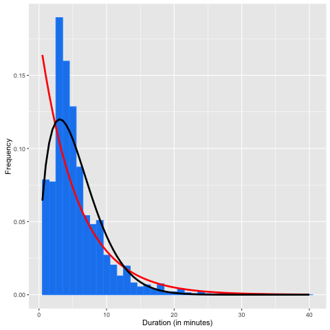
(a) Pre-peak duration

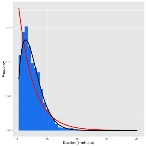
(b) Post-peak duration

Figure 1: Histograms of duration for pre/post-peak durations. Empirical bayes pdfs for exponential (red) and weibull (black) densities are overlayed.

We next examine the pre and post peak durations. Under the Markovian model, the duration of each period is exponentially distributed. Figure 1 shows histograms of the duration of pre and post peak durations in the analyzed subset of data along with empirical Bayes estimates of the probability density functions under both exponential and Weibull distribution specifications. We recognize the durations are discrete and the above distributions are continuous. These are fit for simplicity. When generating the episode duration we generate a random variable from the continuous distribution and take the integer part of that random variable. It is evident from the figures that the Weibull distribution is more appropriate. This is supported by data analysis presented below.

Table 6 presents the parameter estimates for this over-fit model to the duration data assuming a Weibull distribution. Like the episodic transition rules, the post and pre peak durations now depend on the current episode classification as well as the prior episode classifications. The exploratory data analysis suggests a semi-Markovian model in which the pre/post peak durations are Weibull distributed, and the state is given by $(X_{t},U_{t},L^{(1)}_{t},L^{(2)}_{t})$ where $L^{(i)}_{t}$ denotes the classification of the $i$th prior episode.

Table 6: Parameter estimates for each Weibull survival regression.

	Pre-peak				Post-peak
Parameter	Estimate	Std. Error	p-value		Estimate	Std. Error	p-value
Intercept	$1.78$	$0.016$	$0.000$		$1.59$	$0.02$	$0.000$
$0$L Stress Ep.	$-0.20$	$0.037$	$0.000$		$0.45$	$0.07$	$0.000$
$1$L Stress Ep.	-	-	-		$-0.21$	$0.058$	$0.004$
$2$L Stress Ep.	-	-	-		$-0.16$	$0.07$	$0.020$
Log(scale)	$-0.24$	$0.015$	$0.000$		$-0.31$	$0.05$	$0.000$

Next we test robustness of the sample size calculator to the semi-Markovian deviations described above. To test the calculator, we generate data using the no-treatment semi-Markov model specified in Appendix G. The data is simulated so that the treatment effect used by the calculator is correct. See Appendix G for a discussion of how this was achieved.

Table 7 presents achieved power under these alternative generative models. We see that the achieved power is well above the pre-specified 80% threshold in each case. Therefore the sample size calculator is robust to such complex deviations from the Markovian generative model. For the given the alternative effect $\beta(t;x)$ and semi-Markov generative model we calculate the standardized effects. These are provided in Table 15 in Appendix F.

Table 7: Estimated power under semi-Markov generative.

	Estimated power
$\bar{\beta}=0.030$	93.6
$\bar{\beta}=0.025$	88.0
$\bar{\beta}=0.020$	93.6

6.5 Adjustments to the simulation-based calculator

In section 6.4 we evaluated the simulation calculator built in section 6.1. Here we make adjustments to the simulation calculator to ensure robustness. First, we note that the simulation calculator is robust to the potential semi-Markovian deviation discussed in Section 6.4.3. Next we make the decision that we are not concerned with lack of robustness to deviations from a time-homogenous transition matrix as discussed in section 6.4.2. Therefore we focus on making the simulation calculator robust to misspecification of Markov transition matrix as discussed in section 6.4.1.

Analysis in section 6.4.1 suggests for the smoking cessation example that the sample size should be set to ensure at least 80% power over a set of feasible choices for the transition matrix $P^{(0)}$. We fix $(\epsilon,\epsilon^{\prime})=(0.01,2)$ to be our tolerance to misspecification of the inputs. For each set of inputs $(W,Z)\in\Omega_{0.01,2}$, we compute a sample size using the simulation calculator built in Section 6.1. The maximum of this set of computed sample sizes is chosen to ensure tolerance to misspecification of the transition matrix. Table 8 presents the sample size under this procedure as well as the achieved minimum power over the set $\Omega_{\epsilon,\epsilon^{\prime}}$.

Table 8: Estimated sample size, $N$, and computed power under $\epsilon=2$ and $\epsilon^{\prime}=0.01$.

	Sample size	Minimum Power
$\bar{\beta}=0.030$	69	81.9
$\bar{\beta}=0.025$	107	80.4
$\bar{\beta}=0.020$	208	80.5

We have now used the three-step procedure to form a sample size calculator for the smoking cessation study example. For illustration suppose we wish to detect an average conditional treatment effect $\bar{\beta}$ equal to $0.025$. Based on the above discussion a sample size, $N$, of $107$ would be recommended to ensure power above the pre-specified 80% threshold across a set of feasible deviations from the assumed generative model.

7 Discussion

In this paper we introduced the “stratified micro-randomized trial” and provided a definition and discussion of proximal treatment effects along with the dependence of this definition on a reference distribution. We proposed a simulation-based approach for determining sample size and used this approach to determine the sample size for a simplified version of the MD2K smoking cessation study. We expect that similar trial designs would be applicable in areas such as marketing and advertising in which each client is tracked and provided incentives, e.g. treatments, repeatedly over time, and it is of interest to determine in which contexts particular treatments are most effective.

While the focus here is sample size considerations, stratified micro-randomized studies yield data for a variety of interesting secondary data analyses. For example, understanding predictors of future availability is of general interest as keeping participants engaged in the mobile health intervention is often of high concern. Moreover, there is interest in using the data in constructing “dynamic treatment regimes” (e.g., just-in-time adaptive interventions (Spruijt-Metz and Nilsen, 2014)). The stratified micro-randomized trial improves such analyses by reducing causal confounding.

Appendix A Randomization probabilities

Here we provide a brief discussion of how the randomization probabilities $p_{t}(a\,|\,H_{t})$ might be calculated. Suppose we require the participant to receive on average a certain number of interventions per day at the various levels of the time varying covariates, $N_{x}$ for $x\in\{0,\dots,k\}:=[k]$. In the smoking cessation example, we have the time-varying covariate taking values in $\mathcal{X}=\{0=\text{Non-stressed},1=\text{Stressed}\}$. We aim for participants to receive on average one and a half interventions per day when classified as stressed and one and a half interventions per day when not classified as stressed. Formally, our randomization algorithm is designed to satisfy the following:

$$\mathbb{E}\left[\sum_{i=1}^{T}A_{t}I_{t}{\bf 1}[X_{t_{i}}=x]\right]=N_{x}$$ (12)

for each $x\in[k]$. The inputs of the randomization algorithm are $\{N_{x}\}$, a tuning parameter $\lambda\in[0,1]$, and a prediction, denoted by $g_{t}(x,r;h)$, at time $t$ of the number of times in state $x$ and available during the remaining time $r$ given data $h$. The probability to assign treatment at time $t$ given $H_{t}$ is given by

$$p_{t}(1\,|\,H_{t})=\frac{N_{X_{t}}-\sum_{s=1}^{t-1}\left[\lambda_{s}A_{s}+(1-\lambda_{s})p_{s}(1\,|\,H_{s})\right]{\bf 1}[X_{s}=X_{t}]}{1+g_{t}(X_{t},T-t;H_{t})}$$ (13)

where $\lambda_{s}=\lambda^{t-s}$. In addition, we restrict the randomization probability within the interval $[\epsilon,1-\epsilon]$.

To derive (13) we start by re-writing equation (12) as

$$\mathbb{E}\left[\sum_{t=1}^{T}A_{t}\mathds{1}_{\{X_{t}=x\}}\right]=\mathbb{E}\left[\sum_{t=1}^{T}p_{t}(1\,|\,H_{t})\mathds{1}_{\{X_{t}=x\}}\right]$$

or for $\lambda_{t}\in(0,1)$,

$$\mathbb{E}\left[\sum_{t=1}^{T}A_{t}\mathds{1}_{\{X_{t}=x\}}\right]=\mathbb{E}\left[\sum_{t=1}^{T}\big{(}\lambda_{t}A_{t}+(1-\lambda_{t})p_{t}(1\,|\,H_{t})\big{)}\mathds{1}_{\{X_{t}=x\}}\right]$$

The conditional expectation of the latter given the current history $H_{s}$ is

$$\mathbb{E}\left[\sum_{t=1}^{T}\big{(}\lambda_{t}A_{t}+(1-\lambda_{t})p_{t}(1\,|\,H_{t})\big{)}\mathds{1}_{\{X_{t}=x\}}\,|\,H_{s}\right]$$

$$= \sum_{t=1}^{s-1}\left(\lambda_{t}A_{t}+(1-\lambda_{t})p_{t}(1\,|\,H_{t})\right)\mathds{1}_{\{X_{t}=x\}}+p_{s}(1\,|\,H_{s})+\mathbb{E}\left[\sum_{t=s+1}^{T}p_{t}(1\,|\,H_{t})\mathds{1}_{\{X_{t}=x\}}\,|\,H_{s}\right]$$

We aim to find $p_{s}(1\,|\,H_{s})$ such that $N_{x}\approx\mathbb{E}[\sum_{t=1}^{T}\left(\lambda_{t}A_{t}+(1-\lambda_{t})p_{t}(1\,|\,H_{t})\right)\mathds{1}_{\{X_{t}=x\}}|H_{s}]$ for each $x\in[k]$. However, at the end of $s$ decision time, we do not have access to future randomization probabilities, i.e. $p_{t}(1\,|\,H_{t})$ under $X_{t}=x$ for $t\geq s+1$, which appears in the last term above. As such, we approximate $p_{t}(1\,|\,H_{t})$ by $p_{s}(1\,|\,H_{s})$ whenever $X_{t}=x$, e.g. using the same randomization probabilities for future time points, and obtain $p_{s}(1\,|\,H_{s})$ by solving:

$$N_{x}=\sum_{t=1}^{s-1}\left(\lambda_{t}A_{t}+(1-\lambda_{t})p_{t}(1\,|\,H_{t})\right)\mathds{1}_{\{X_{t}=x\}}+p_{s}(1\,|\,H_{s})+\mathbb{E}\left[\sum_{t=s+1}^{T}p_{s}(1\,|\,H_{s})\mathds{1}_{\{X_{t}=x\}}\,|\,H_{s}\right]$$

That is,

$$p_{s}(1\,|\,H_{s})=\frac{N_{x}-\sum_{t=1}^{s-1}\left[\lambda_{t}A_{t}+(1-\lambda_{t})p_{t}(1\,|\,H_{t})\right]\mathds{1}_{\{X_{t}=x\}}}{1+\mathbb{E}\left[\sum_{t=s+1}^{T}\mathds{1}_{\{X_{t}=x\}}\,|\,H_{s}\right]}$$

The remaining problem is to approximate $g_{t}(1,T-s;H_{s})=\mathbb{E}\left[\sum_{t=s+1}^{T}\mathds{1}_{\{X_{t}=1\}}\,|\,H_{s}\right]$, which is, at time $s$, the expected total number of future, available time points classified as $x$ given the current history. This approximation is essentially a prediction problem. There are a variety of approaches one can take depending on the data available. These prediction approaches may use distributional assumptions, such as Markovian assumptions, on $X_{t}$ if there is only a small amount of data to form these predictions or can employ more black box predictions if there is a great deal of data. In the actual smoking cessation study, there was only a small amount of pre-existing data so a Markovian model was used to form the predictions. For the smoking cessation study example, we set $N=(1.65,2.15)$, $\lambda=0.3$, $\epsilon=0.001$ and the remainder function is set according to following rule:

• If $(T-t)-N_{x}\cdot 60<60$ then set $g_{t}(x,T-t;H_{t})=(T-t)\pi_{x}$,

• else if $(T-t)-N_{x}\cdot 60<120$ then set $g_{t}(x,T-t;H_{t})=(T-t-60)\pi_{x}$,

• else set $g_{t}(x,T-t;H_{t})=(T-t-120)\pi_{x}$,

where $\pi$ is the stationary distribution of the markov transition matrix $P^{(0)}$. The reason for this complex rule is we must incorporate the fact that a participant is unavailable for the hour following delivery of an intervention.

Appendix B Technical Arguments

B.1 Treatment effects under potential outcomes framework

Proof of Lemma 3.3.

We establish Lemma 3.3 for the marginal treatment effect. The argument for the conditional treatment effect follows from a similar argument.

For $a\in\{0,1\}$, we consider the

$$\mathbb{E} \left[\left(\prod_{j=1}^{t-1}p_{j}(a_{j}|H_{j}(\bar{a}_{j-1}))\right)Y_{t,\Delta}(\bar{a}_{t-1},a,\bar{0})I_{t}(\bar{a}_{t-1})\right]$$

$$=\mathbb{E} \left[\left(\prod_{j=1}^{t-1}p_{j}(a_{j}|H_{j}(\bar{a}_{j-1}))\right)I_{t}(\bar{a}_{t-1})\mathbb{E}\left[Y_{t,\Delta}(\bar{a}_{t-1},a,\bar{0})\,|\,H_{t}(\bar{a}_{t-1})\right]\right]$$

Since the history $H_{t}$ includes availability at time $t$. By consistency, $H_{t}(\bar{A}_{t-1})=H_{t}$ and $I_{t}(\bar{a}_{t-1})=I_{t}$ so the above is equal to

$$\mathbb{E}\left[\left(\prod_{j=1}^{t-1}p_{j}(a_{j}|H_{j})\right)I_{t}\mathbb{E}\left[Y_{t,\Delta}(\bar{a}_{t-1},a,\bar{0})\,|\,H_{t}\right]\right]$$ (14)

Sequential ignorability implies that

$$\mathbb{E} \left[Y_{t,\Delta}(\bar{a}_{t-1},a,\bar{0})\,|\,H_{t}\right]$$

$$=\mathbb{E} \left[Y_{t,\Delta}(\bar{a}_{t-1},a,\bar{0})\,|\,H_{t},A_{t}=a\right]$$

Sequential ignorability also implies that $\mathbb{E}[Y_{t,\Delta}(\bar{a}_{t-1},a,\bar{0})\,|\,H_{t+k}]\mathbb{E}[1_{A_{t+k}=0}\,|\,H_{t+k}]$ is equal to $\mathbb{E}[Y_{t,\Delta}(\bar{a}_{t-1},a,\bar{0})1_{A_{t+k}=0}\,|\,H_{t+k}]$. We apply this to show

$$\mathbb{E} \left[Y_{t,\Delta}(\bar{a}_{t-1},a_{t},\bar{0})\,|\,H_{t},A_{t}=a\right]$$

$$=\mathbb{E} \left[\mathbb{E}\left[Y_{t,\Delta}(\bar{a}_{t-1},a_{t},\bar{0})\,|\,H_{t+1}\right]\,|\,H_{t},A_{t}=a\right]$$

$$=\mathbb{E} \left[\mathbb{E}\left[Y_{t,\Delta}(\bar{a}_{t-1},a_{t},\bar{0})\,|\,H_{t+1}\right]\frac{\mathbb{E}[1_{A_{t+1}=0}\,|\,H_{t+1}]}{p_{t+1}(0\,|\,H_{t+1})}\,|\,H_{t},A_{t}=a\right]$$

$$=\mathbb{E} \left[\mathbb{E}\left[Y_{t,\Delta}(\bar{a}_{t-1},a_{t},\bar{0})\frac{1_{A_{t+1}=0}}{p_{t+1}(0\,|\,H_{t+1})}\,|\,H_{t+1}\right]\,|\,H_{t},A_{t}=a\right]$$

Iteratively applying this argument, we end up with the following expectation

$$\mathbb{E}\bigg{[}\frac{1_{A_{t+1}=0}}{p_{t+1}(0\,|\,H_{t+1})}\mathbb{E} \left[\cdots\mathbb{E}\left[Y_{t,\Delta}(\bar{a}_{t-1},a_{t},\bar{0})\frac{1_{A_{t+\Delta-1}=0}}{p_{t+\Delta-1}(0\,|\,H_{t+\Delta-1})}\,|\,H_{t+\Delta-1}\right]\,|\,H_{t+1}\right]\,|\,H_{t},A_{t}=a\bigg{]}$$

$$=\mathbb{E}\left[\prod_{j=t+1}^{t+\Delta-1}\frac{1_{A_{j}=0}}{p_{j}(0\,|\,H_{j})}\,Y_{t,\Delta}(\bar{a}_{t-1})\,|\,H_{t},A_{t}=a\right]$$

Plugging this result into equation (14), we have

$$\mathbb{E}\left[\left(\prod_{j=1}^{t-1}p_{j}(a_{j}|H_{j})\right)I_{t}\mathbb{E}\left[\prod_{j=t+1}^{t+\Delta-1}\frac{1_{A_{j}=0}}{p_{j}(0\,|\,H_{j})}\,Y_{t,\Delta}(\bar{a}_{t-1})\,|\,H_{t},A_{t}=a\right]\,\right].$$

Summing over all potential outcomes $\bar{a}_{t-1}$ and normalizing yields

$$\mathbb{E} \left[\sum_{\bar{a}_{t-1}}\frac{\left(\prod_{j=1}^{t-1}p_{j}(a_{j}|H_{j})\right)I_{t}}{\mathbb{E}[\sum_{\bar{a}_{t-1}}\left(\prod_{j=1}^{t-1}p_{j}(a_{j}|H_{j})\right)I_{t}]}\mathbb{E}\left[\prod_{j=t+1}^{t+\Delta-1}\frac{1_{A_{j}=0}}{p_{j}(0\,|\,H_{j})}\,Y_{t,\Delta}(\bar{a}_{t-1})\,|\,H_{t},A_{t}=a\right]\,\right]$$

$$=\mathbb{E} \left[\sum_{\bar{a}_{t-1}}\frac{\left(\prod_{j=1}^{t-1}p_{j}(a_{j}|H_{j})\right)I_{t}}{\mathbb{E}[\sum_{\bar{a}_{t-1}}\left(\prod_{j=1}^{t-1}p_{j}(a_{j}|H_{j})\right)I_{t}]}\mathbb{E}\left[\prod_{j=t+1}^{t+\Delta-1}\frac{1_{A_{j}=0}}{p_{j}(0\,|\,H_{j})}\,Y_{t,\Delta}(\bar{a}_{t-1})\,|\,H_{t},A_{t}=a\right]\,|\,I_{t}=1\right]$$

$$=\mathbb{E} \left[\mathbb{E}\left[\prod_{j=t+1}^{t+\Delta-1}\frac{1_{A_{j}=0}}{p_{j}(0\,|\,H_{j})}\,Y_{t,\Delta}\,|\,H_{t},A_{t}=a\right]\,|\,I_{t}=1\right].$$

In the final equation, the outer expectation is with respect to the history $H_{t}$ conditional on $I_{t}=1$. That is, over both past actions $A_{s}$ and past observations $O_{s}$ for $s<t$.

The above shows

$$\frac{\mathbb{E}\left[\left(\prod_{j=1}^{t-1}p_{j}(a_{j}|H_{j}(\bar{a}_{j-1}))\right)Y_{t,\Delta}(\bar{a}_{t-1},a,\bar{0})I_{t}(\bar{a}_{t-1})\right]}{\mathbb{E}\left[\left(\prod_{j=1}^{t-1}p_{j}(a_{j}|H_{j}(\bar{a}_{j-1}))\right)I_{t}(\bar{a}_{t-1})\right]}$$

$$= \mathbb{E}\left[\mathbb{E}\left[\prod_{j=t+1}^{t+\Delta-1}\frac{1_{A_{j}=0}}{p_{j}(0\,|\,H_{j})}\,Y_{t,\Delta}\,|\,H_{t},A_{t}=a\right]\,|\,I_{t}=1\right]$$

which completes the proof. ∎

B.2 Asymptotic consistency and normality

We provide a detailed proof of asymptotic normality and consistency in the conditional setting for the weighted-centered least squares estimator. The proof in the marginal setting follows in a similar manner with only minor modification. For ease of notation, we write $\mathbb{E}_{\bf p}$ to denote expectations where the distribution over actions is with respect to the randomization probability ${P}_{\bf p}$, and $\mathbb{E}_{\eta}$ to denote expectations where the distribution over actions is with respect to the chosen reference distribution – that is, providing a prompt at time $t$ with probability $\tilde{p}_{t}(1\,|\,X_{t})$ followed by no prompt over the next hour.

Lemma B.1 (Change from randomization probability to reference distribution).

For any function $\phi(H_{t+k})$ of the history up to time $t+k$, for $k\geq 0$,

$$\mathbb{E}_{\bf p}\left[w_{ct}(H_{t+\Delta-1})\phi(H_{t+k})\,|\,H_{t}\right]=\mathbb{E}_{\eta}\left[\phi(H_{t+k})\,|\,H_{t}\right]$$

where

$$w_{ct}(H_{t+\Delta-1})=\frac{\tilde{p}_{t}(A_{t}|X_{t}){\prod_{s=1}^{\Delta-1}}{\bf 1}[A_{t+s}=0]}{\prod_{s=0}^{\Delta-1}p_{t+s}(A_{t+s}\,|\,H_{t+s})}.$$

Proof of Lemma B.1.

Suppose $\Delta=2$. Then

$$\mathbb{E}_{\bf p}\left[w_{ct}(H_{t+\Delta-1})\phi(H_{t+k})\,|\,H_{t}\right]$$

$$= \mathbb{E}_{\bf p}\left[\frac{\tilde{p}_{t}(A_{t}|X_{t})}{p_{t}(A_{t}\,|\,H_{t})}\mathbb{E}\left[\frac{{\bf 1}[A_{t+1}=0]}{p_{t+1}(A_{t+1}\,|\,H_{t+1})}\phi(H_{t+k})\,|\,H_{t+1},A_{t+1}\right]\,|\,H_{t}\right]$$

$$= \mathbb{E}\left[\frac{\tilde{p}_{t}(A_{t}|X_{t})}{p_{t}(A_{t}\,|\,H_{t})}\sum_{a}\frac{{\bf 1}(a=0)}{\pi(A_{t+1}=a\,|\,H_{t+1})}\pi(A_{t+1}=a\,|\,H_{t+1})\mathbb{E}\left[\phi(H_{t+k})\,|\,H_{t+1},A_{t+1}=a\right]\,|\,H_{t}\right]$$

$$= \mathbb{E}\left[\frac{\tilde{p}_{t}(A_{t}|X_{t})}{p_{t}(A_{t}\,|\,H_{t})}\sum_{a}{\bf 1}[a=0]\cdot\mathbb{E}\left[\phi(H_{t+k})\,|\,H_{t+1},A_{t+1}=a\right]\,|\,H_{t}\right]$$

$$= \mathbb{E}\left[\frac{\tilde{p}_{t}(A_{t}|X_{t})}{p_{t}(A_{t}\,|\,H_{t})}{\bf 1}[A_{t+1}=0]\mathbb{E}\left[\phi(H_{t+k})\,|\,H_{t+1},A_{t+1}\right]\,|\,H_{t}\right]$$

$$= \sum_{a}\frac{\tilde{p}_{t}(A_{t}=a|X_{t})}{p_{t}(A_{t}=a\,|\,H_{t})}p_{t}(A_{t}=a\,|\,H_{t})\mathbb{E}\left[{\bf 1}[A_{t+1}=0]\mathbb{E}\left[\phi(H_{t+k})\,|\,H_{t+1},A_{t+1}\right]\,|\,H_{t}\right]$$

$$= \sum_{a}\tilde{p}_{t}(A_{t}=a|X_{t})\mathbb{E}\left[{\bf 1}[A_{t+1}=0]\phi(H_{t+k})\,|\,H_{t}\right]$$

Applying this argument iteratively leads

$$\sum_{a}\tilde{p}_{t}(A_{t}=a|X_{t})\mathbb{E}\left[\left(\prod_{j=1}^{\Delta}{\bf 1}[A_{t+j}=0]\right)\phi(H_{t+k})\,|\,H_{t},A_{t}=a\right]=\mathbb{E}_{\eta}\left[\phi(H_{t+k})\,|\,H_{t}\right]$$

as desired. ∎

Lemma B.1 yields many important corollaries. First,

$$\mathbb{E}_{\bf p}[w_{ct}(H_{t+\Delta-1})\,|\,H_{t}]=\mathbb{E}_{\eta}[1\,|\,H_{t}]=1,$$

which implies $\mathbb{E}_{\bf p}[w_{ct}(H_{t+\Delta-1})\,|\,X_{t}]=1$. Also, define

$$\mathbb{E}_{\bf p}[w_{ct}(H_{t+\Delta-1})Y_{t,\Delta}\,|\,H_{t}]=\mathbb{E}_{\eta}[Y_{t,\Delta}\,|\,H_{t}]=\alpha(t;H_{t})$$

Lemma B.2.

For any $k\geq 0$ and function $\phi(H_{t+k})$, we have

$$\mathbb{E}_{\bf p} [w_{ct}(H_{t+\Delta-1})\big{(}A_{t}-\tilde{p}_{t}(1\,|\,X_{t})\big{)}\phi(H_{t+k})\,|\,X_{t}]$$

$$=\tilde{p}_{t}(1\,|\,X_{t})(1-\tilde{p}_{t}(1\,|\,X_{t}))\mathbb{E}\left[\Big{(}\mathbb{E}_{\eta}[\phi(H_{t+k})\,|\,H_{t},A_{t}=1]-\mathbb{E}_{\eta}[\phi(H_{t+k})\,|\,H_{t},A_{t}=0]\Big{)}\,|\,X_{t}\right]$$

In particular, we have $\mathbb{E}_{\bf p}[w_{ct}(H_{t+\Delta-1})Y_{t,\Delta}(A_{t}-\tilde{p}_{t}(1\,|\,X_{t}))\,|\,X_{t}=x]=\tilde{p}_{t}(1\,|\,X_{t})(1-\tilde{p}_{t}(1\,|\,X_{t}))\beta(t;X_{t})$. Note that if $\phi(H_{t+k})$ is a constant function of $H_{t}$ and $A_{t}$ then the above expression is equal to zero.

Proof.

$$\mathbb{E}_{\bf p}[w_{ct}(H_{t+\Delta-1})\left(A_{t}-\tilde{p}_{t}(1\,|\,X_{t})\right)\phi(H_{t+k})\,|\,X_{t}]$$

$$= \mathbb{E}_{\bf p}\left[\frac{\tilde{p}_{t}(A_{t}|X_{t})}{p_{t}(A_{t}|H_{t})}\left(A_{t}-\tilde{p}_{t}(1\,|\,X_{t})\right)\mathbb{E}_{\bf p}\left[\frac{{\prod_{s=1}^{\Delta-1}}{\bf 1}[A_{t+s}=0]}{\prod_{s=1}^{\Delta-1}p_{t+s}(A_{t+s}\,|\,H_{t+s})}\phi(H_{t+k})\,|\,H_{t},A_{t}\right]\,|\,X_{t}\right]$$

$$= \mathbb{E}_{\bf p}\left[\sum_{a\in\{0,1\}}\frac{\tilde{p}_{t}(A_{t}\,|\,X_{t})}{p_{t}(A_{t}\,|\,H_{t})}p_{t}(A_{t}\,|\,H_{t})\left(a-\tilde{p}_{t}(1\,|\,X_{t})\right)\mathbb{E}_{\bf p}\left[\frac{{\prod_{s=1}^{\Delta-1}}{\bf 1}[A_{t+s}=0]}{\prod_{s=1}^{\Delta-1}p_{t+s}(A_{t+s}\,|\,H_{t+s})}\phi(H_{t+k})\,|\,H_{t},A_{t}=a\right]\,|\,X_{t}\right]$$

$$= \tilde{p}_{t}(1\,|\,X_{t})\left(1-\tilde{p}_{t}(1\,|\,X_{t})\right)\mathbb{E}\left[\mathbb{E}_{\eta}\left[\phi(H_{t+k})\,|\,H_{t},A_{t}=1\right]-\mathbb{E}_{\eta}\left[\phi(H_{t+k})\,|\,H_{t},A_{t}=0\right]\,|\,X_{t}\right]$$

If $\phi(H_{t+k})=w_{t+1,\Delta}Y_{t,\Delta}$, then by Lemma B.1 the above equals

$$\tilde{p}_{t}(1\,|\,X_{t})\left(1-\tilde{p}_{t}(1\,|\,X_{t})\right) \mathbb{E}\left[\mathbb{E}_{\eta}\left[Y_{t,\Delta}\,|\,H_{t},A_{t}=1\right]-\mathbb{E}_{\eta}\left[Y_{t,\Delta}\,|\,H_{t},A_{t}=0\right]\,|\,X_{t}\right]$$

$$=\tilde{p}_{t}(1\,|\,X_{t})\left(1-\tilde{p}_{t}(1\,|\,X_{t})\right) \mathbb{E}\bigg{[}\mathbb{E}_{\bf p}\left[\frac{{\prod_{s=1}^{\Delta-1}}{\bf 1}[A_{t+s}=0]}{\prod_{s=1}^{\Delta-1}p_{t+s}(A_{t+s}\,|\,H_{t+s})}\phi(H_{t+k})\,|\,H_{t},A_{t}=1\right]$$

$$- \mathbb{E}_{\bf p}\left[\frac{{\prod_{s=1}^{\Delta-1}}{\bf 1}[A_{t+s}=0]}{\prod_{s=1}^{\Delta-1}p_{t+s}(A_{t+s}\,|\,H_{t+s})}\phi(H_{t+k})\,|\,H_{t},A_{t}=0\right]\,|\,X_{t}\bigg{]}$$

$$=\tilde{p}_{t}(1\,|\,X_{t})\left(1-\tilde{p}_{t}(1\,|\,X_{t})\right) \beta(t;X_{t})$$

as desired. ∎

Lemma B.2 implies the function $\tilde{p}_{t}$ must be conditionally independent of $H_{t}$ given $X_{t}$ in order to guarantee a consistent estimator of the projection of $\beta^{\star}_{c}$.

Lemma B.3.

The solutions $(\hat{\alpha},\hat{\beta})$ that minimize equation (6) are consistent estimators for:

$$\alpha^{\star} =\left(\mathbb{E}\left[\sum_{t=1}^{T}g_{t}(H_{t})g_{t}(H_{t})^{\prime}\right]\right)^{-1}\mathbb{E}\left[\sum_{t=1}^{T}g_{t}(H_{t})\alpha(t;H_{t})\right]$$

$$\beta^{\star} =\left(\mathbb{E}\left[\sum_{t=1}^{T}\tilde{\sigma}_{t}^{2}(X_{t})f_{t}(X_{t})f_{t}(X_{t})^{\prime}\right]\right)^{-1}\mathbb{E}\left[\sum_{t=1}^{T}\tilde{\sigma}_{t}^{2}(X_{t})f_{t}(X_{t})\beta(t;X_{t})\right]$$

where $\tilde{\sigma}_{t}^{2}(X_{t})=\tilde{p}_{t}(1\,|\,X_{t})(1-\tilde{p}_{t}(1\,|\,X_{t}))$.

Proof.

The solutions $(\hat{\alpha},\hat{\beta})$ that minimize equation (6) are consistent estimators for the solutions that minimize the following

$$\mathbb{E}\left[\sum_{t=1}^{T}w_{ct}(H_{t+\Delta})\left(Y_{t,\Delta}-g_{t}(H_{t})^{\prime}\alpha^{\star}-(A_{t}-\tilde{p}_{t}(1\,|\,X_{t}))f_{t}(X_{t})^{\prime}\beta^{\star}\right)^{2}\right]$$

Differentiating the above equation with respect to $\alpha^{\star}$ yields a set of $p$ estimating equations.

$$0_{q^{\prime}} =\mathbb{E}_{\bf p}\left[\sum_{t=1}^{T}w_{ct}(H_{t+\Delta-1})\left(Y_{t,\Delta}-g_{t}(H_{t})^{\prime}\alpha^{\star}-(A_{t}-\tilde{p}_{t}(1\,|\,X_{t}))f_{t}(X_{t})^{\prime}\beta^{\star}\right)g_{t}(H_{t})\right]$$

$$=\sum_{t=1}^{T}\mathbb{E}\left[\mathbb{E}_{\bf p}\left[w_{ct}(H_{t+\Delta-1})\left(Y_{t,\Delta}-g_{t}(H_{t})^{\prime}\alpha^{\star}-(A_{t}-\tilde{p}_{t}(1\,|\,X_{t}))f_{t}(X_{t})^{\prime}\beta^{\star}\right)\,|\,H_{t}\right]g_{t}(H_{t})\right]$$

By Lemma B.2, $\mathbb{E}_{\bf p}\left[w_{ct}(H_{t+\Delta})(A_{t}-\tilde{p}_{t}(1\,|\,X_{t}))f_{t}(X_{t})^{\prime}\beta^{\star}\,|\,H_{t}\right]=0$. Therefore, we have,

$$0_{q^{\prime}} =\sum_{t=1}^{T}\mathbb{E}\left[\mathbb{E}_{\bf p}\left[w_{ct}(H_{t+\Delta-1})\left(Y_{t,\Delta}-g_{t}(H_{t})^{\prime}\alpha^{\star}\right)\,|\,H_{t}\right]g_{t}(H_{t})\right]$$

$$=\sum_{t=1}^{T}\mathbb{E}\left[g_{t}(H_{t})\alpha(t;H_{t})-g_{t}(H_{t})g_{t}(H_{t})^{\prime}\alpha^{\star}\right]$$

and we have the desired equivalence. The second equality is due to Lemma B.1. Now differentiating with respect to $\beta^{\star}$ yields

$$0_{q_{c}} =\mathbb{E}_{\bf p}\left[\sum_{t=1}^{T}w_{ct}(H_{t+\Delta-1})\left(Y_{t,\Delta}-g_{t}(H_{t})^{\prime}\alpha^{\star}-(A_{t}-\tilde{p}_{t}(1\,|\,X_{t}))f_{t}(X_{t})^{\prime}\beta^{\star}\right)(A_{t}-\tilde{p}_{t}(1\,|\,X_{t}))f_{t}(X_{t})\right]$$

By Lemma B.2, we have $\mathbb{E}_{\bf p}\left[w_{ct}(H_{t+\Delta-1})(A_{t}-\tilde{p}_{t}(1\,|\,X_{t}))Y_{t,\Delta}\,|\,H_{t}\right]=\tilde{p}_{t}(1\,|\,X_{t})(1-\tilde{p}_{t}(1\,|\,X_{t}))\beta_{\eta}(t;X_{t})$, and $\mathbb{E}_{\bf p}\left[w_{t}(H_{t+\Delta-1})(A_{t}-\tilde{p}_{t}(1\,|\,X_{t}))g_{t}(H_{t})\,|\,H_{t}\right]=0$. The final term satisfies

$$\mathbb{E}_{\bf p}\left[w_{t}(H_{t+\Delta-1})(A_{t}-\tilde{p}_{t}(1\,|\,X_{t}))^{2}\,|\,H_{t}\right]=\tilde{p}_{t}(1\,|\,X_{t})(1-\tilde{p}_{t}(1\,|\,X_{t}))=\tilde{\sigma}_{t}^{2}(X_{t})$$

by Lemma B.1. Then we have

$$0_{q} =\sum_{t=1}^{T}\mathbb{E}\left[\tilde{\sigma}_{t}^{2}(X_{t})f_{t}(X_{t})\beta_{\eta}(t;X_{t})-\tilde{\sigma}_{t}^{2}(X_{t})f_{t}(X_{t})f_{t}(X_{t})^{\prime}\beta^{\star}\right]$$

as desired. ∎

Proof of Asymptotic Normality in Lemma 4.1.

We now consider the issue of asymptotic normality. First, let

$$\epsilon_{ct}=Y_{t,\Delta}-g_{t}(H_{t})^{\prime}\alpha^{\star}-(A_{t}-\tilde{p}_{t}(X_{t}))f_{t}(X_{t})^{\prime}\beta^{\star},$$

$\hat{\theta}=(\hat{\alpha},\hat{\beta})$, and $\theta^{\star}=(\alpha^{\star},\beta^{\star})$. Since $X_{t}\subset H_{t}$ we define $h_{t}(H_{t})^{\prime}=(g_{t}(H_{t})^{\prime},(A_{t}-\tilde{p}_{t}(1\,|\,X_{t}))f_{t}(X_{t})^{\prime})$. Then

$$\sqrt{N}(\hat{\theta}-\theta^{\star}) =\sqrt{N}\bigg{\{}\bigg{(}\mathbb{P}_{N}\sum_{t=1}^{T}w_{ct}(H_{t+\Delta-1})h_{t}(H_{t})h_{t}(H_{t})^{\prime}\bigg{)}^{-1}\bigg{[}\bigg{(}\mathbb{P}_{N}\sum_{t=1}^{T}Y_{t,\Delta}w_{ct}(H_{t+\Delta-1})h_{t}(H_{t})\bigg{)}$$

$$-\bigg{(}\mathbb{P}_{N}\sum_{t=1}^{T}w_{ct}(H_{t+\Delta-1})h_{t}(H_{t})h_{t}(H_{t})^{\prime}\bigg{)}\theta^{\star}\bigg{]}\bigg{\}}$$

$$=\sqrt{N}\bigg{\{}E\bigg{[}\sum_{t=1}^{T}w_{ct}(H_{t+\Delta-1})h_{t}(H_{t})h_{t}(H_{t})^{\prime}\bigg{]}^{-1}$$

$$\bigg{[}\bigg{(}\mathbb{P}_{N}\sum_{t=1}^{T}w_{ct}(H_{t+\Delta-1})\epsilon_{ct}h_{t}(H_{t})\bigg{)}\bigg{]}\bigg{\}}+o_{p}({\bf 1})$$

By definitions of $\alpha^{\star}$ and $\beta^{\star}$ and the previous consistency argument

$$E\left[\sum_{t=1}^{T}w_{ct}(H_{t+\Delta-1})\epsilon_{ct}h_{t}(H_{t})\right]=0$$

Then under moments conditions, we have asymptotic normality with variance $\Sigma_{\theta}$ given by

$$\Sigma_{\theta} =E\left[\sum_{t=1}^{T}w_{ct}(H_{t+\Delta-1})h_{t}(X_{t})h_{t}(X_{t})^{\prime}\right]^{-1}$$

$$E\left[\sum_{t=1}^{T}w_{ct}(H_{t+\Delta-1})\epsilon_{ct}h_{t}(X_{t})\times\sum_{t=1}^{T}w_{ct}(H_{t+\Delta-1})\epsilon_{ct}h_{t}(X_{t})^{\prime}\right]$$

$$E\left[\sum_{t=1}^{T}w_{ct}(H_{t+\Delta-1})h_{t}(X_{t})h_{t}(X_{t})^{\prime}\right]^{-1}$$

Due to centering and the previous lemma, the expectation of the matrix $w_{ct}(H_{t+\Delta-1})h_{t}(X_{t})h_{t}(X_{t})^{\prime}$ is block diagonal and therefore, we can extract the sub-covariance matrix $\Sigma_{\beta}$ “cleanly” from the above formula. Using this, we have

$$\Sigma_{\beta} =\left[\sum_{t=1}^{T}E[(A_{t}-\tilde{p}_{t}(X_{t}))^{2}w_{t}(H_{t+\Delta})f_{t}(X_{t})f_{t}(X_{t})^{\prime}]\right]^{-1}$$

$$\cdot E\bigg{[}\sum_{t=1}^{T}w_{t}(H_{t+\Delta})\epsilon_{ct}(A_{t}-\tilde{p}_{t}(X_{t}))f_{t}(X_{t})\times\sum_{t=1}^{T}w_{t}(H_{t+\Delta})\epsilon_{ct}(A_{t}-\tilde{p}_{t}(X_{t}))f_{t}(X_{t})^{\prime}\bigg{]}$$

$$\,\cdot\left[\sum_{t=1}^{T}E[(A_{t}-\tilde{p}_{t}(X_{t}))^{2}w_{t}(H_{t+\Delta})f_{t}(X_{t})f_{t}(X_{t})^{\prime}\right]^{-1}$$

as desired. ∎

Proof of asymptotic distribution of $T_{cN}$.

By the above proof, we have

$$\sqrt{N}(\hat{\beta}_{c}-\beta^{\star}_{c})^{\prime}\to N(0,\Sigma)$$

where $\Sigma=Q^{-1}WQ^{-1}$, as defined in Lemma 4.1. Since a quadratic form of the normal distribution has a chi-square distribution, we have

$$N(\hat{\beta}_{c}-\beta^{\star}_{c})^{\prime}\Sigma^{-1}(\hat{\beta}_{c}-\beta^{\star}_{c})\to\chi^{2}_{q_{c}}.$$

$T_{cN}$ replaces $\Sigma$ with a consistent estimator $\hat{\Sigma}$. By independence of the covariance estimator and the equation above, we have

$$q_{c}^{-1}N(\hat{\beta}_{c}-\beta^{\star}_{c})^{\prime}\hat{\Sigma}^{-1}(\hat{\beta}_{c}-\beta^{\star}_{c})\sim^{a}F(q_{c},N-q^{\prime}-q_{c}).$$

For large $N$, we have the F-distribution with degrees of freedom $q_{c}$ and $N-q^{\prime}-q$ is well approximated by a multiple of the $\chi^{2}$-distribution with degree of freedom $q_{c}$; that is, if $X_{N}\sim F(q_{c},N-q^{\prime}-q_{c})$ then $Y=\lim_{N\to\infty}q_{c}X_{N}$ has a chi-square distribution with degrees of freedom $q_{c}$.

For large $N$, asymptotic normality implies $\hat{\beta}_{c}$ has an approximate normal distribution with mean $\beta^{\star}_{c}$ and variance $\Sigma/N$. This implies that $\hat{\beta}_{c}\Sigma^{-1}\hat{\beta}_{c}$ has an approximate non-central chi-square distribution with degrees of freedom $q_{c}$ and non-centrality parameter $\beta^{\star}_{c}\Sigma^{-1}\beta^{\star}_{c}$. That is,

$$N\cdot\hat{\beta}_{c}\Sigma^{-1}\hat{\beta}_{c}\sim^{a}\chi^{2}_{q_{c}}(N\beta^{\star}_{c}\Sigma^{-1}\beta^{\star}_{c})$$

where $\sim^{a}$ means approximately in distribution for large $N$. As $\hat{\Sigma}^{-1}$ is a consistent estimator of $\Sigma$, this implies that

$$T_{cN}=N\hat{\beta}_{c}\hat{\Sigma}^{-1}\hat{\beta}_{c}\sim^{a}q_{c}F(q_{c},N-q^{\prime}-q;\beta^{\star}_{c}\Sigma^{-1}\beta^{\star}_{c}).$$

That is, $\frac{1}{q_{c}}T_{cN}$ has an approximate non-central F-distribution. ∎

Appendix C Tradeoff between approximation error and degrees of freedom for sample size calculations

This section provides a discussion of two tradeoffs involved in attempting to reduce the required sample size for a given power. The first tradeoff involves the complexity of the projection of the treatment effect and the second tradeoff involves the complexity of the projection involving the control variables. For expositional simplicity, we discuss the tradeoffs in the case of sample size calculations for marginal treatment effects. We make the simplifying assumptions that the proximal response is a known function of the participant’s data within a window of length $\Delta=1$ and that the participant is always available for treatment (i.e., $I_{t}=1$ for all $t=1,\ldots,T$).

In the marginal setting, the sample size is the smallest integer $N$ that satisfies:

$$1-F_{q_{m},N-(q^{\prime}+q_{m});N\gamma_{m}}\left(\frac{N-(q^{\prime}+1)}{N-(q^{\prime}+q_{m})}F^{-1}_{q_{m},N-(q^{\prime}+q_{m});0}(1-\alpha_{0})\right)\geq 1-\beta_{0}.$$ (15)

where $\gamma_{m}$ is the non-centrality parameter equal to $(\beta^{\star}_{m})^{\prime}Q_{m}W_{m}^{-1}Q_{m}\beta_{m}^{\star}$ with

$$W_{m}=\mathbb{E}\bigg{[}\sum_{t=1}^{T}w_{mt}(H_{t})\,{\epsilon}_{mt}(A_{t}-\tilde{p}_{t}(1))f_{t} \times\sum_{t=1}^{T}w_{mt}(H_{t})\,{\epsilon}_{mt}(A_{t}-\tilde{p}_{t}(1))f_{t}^{\prime}\bigg{]},$$

$$Q_{m}=\sum_{t=1}^{T}\tilde{p}_{t}(1)(1-\tilde{p}_{t}(1)) f_{t}\,f_{t}^{\prime},\text{ and }w_{mt}(H_{t})=\frac{\tilde{p}_{t}(A_{t})}{p_{t}(A_{t}\,|\,H_{t})},$$

and $\epsilon_{mt}=Y_{t,\Delta}-g_{t}(H_{t})^{\prime}\alpha_{m}^{\star}-(A_{t}-\tilde{p}_{t}(1))f_{t}^{\prime}\beta_{m}^{\star}$. $F_{d_{1},d_{2};\lambda}$ and $F^{-1}_{d_{1},d_{2};\lambda}$ denote the cumulative and inverse distribution functions respectively for the non-central $F$-distribution with degrees of freedom $(d_{1},d_{2})$ and non-centrality parameter $\lambda$.

Define the error term, $\epsilon_{t}$, by

$$\epsilon_{t}=Y_{t,\Delta}-E[w_{mt}(H_{t})Y_{t,\Delta}\mid H_{t}]-(A_{t}-\tilde{p}_{t}(1))\beta(t).$$

The error term has conditional mean zero; that is, $\mathbb{E}[\epsilon_{t}\,|\,H_{t},A_{t}]=0$. See Appendix C.1 for the derivation. Importantly we can write $\epsilon_{mt}$ in terms of the error term $\epsilon_{t}$:

$$\epsilon_{mt} =\epsilon_{t}+\left(E[w_{mt}(H_{t})Y_{t,\Delta}\mid H_{t}]-g_{t}(H_{t})^{\prime}\alpha^{\star}_{m}\right)+(A_{t}-\tilde{p}_{t}(1))\left(\beta(t)-f_{t}^{\prime}\beta_{m}^{\star}\right)$$

$$=\epsilon_{t}+e_{\alpha}(t;H_{t})+(A_{t}-\tilde{p}_{t}(1))e_{\beta}(t).$$

The term $e_{\alpha}(t;H_{t})$ is the approximation error related to the complexity of the $L_{2}$ projection involving the control variables. The term $e_{\beta}(t)$ is the approximation error related to the complexity of the $L_{2}$ projection of the treatment effect.

The goal of the remainder of this section is to provide an intuitive understanding of the tradeoff among the errors due to $L_{2}$ projections (i.e., $e_{\alpha}(t;H_{t})$ and $e_{\beta}(t)$), sample size, and power. We start by forming an approximate sample size formula based on equation (15). In particular when $N$ and $q_{m}$ are large the sample size can be approximated by

$$\gamma_{m}^{-1}\left(2\cdot z_{1-\beta_{0}}^{2}+\sqrt{2q_{m}}z_{1-\alpha_{0}}+2z_{1-\beta_{0}}\sqrt{z_{1-\beta_{0}}^{2}+q_{m}/2+\sqrt{2q_{m}}z_{1-\alpha_{0}}}\right).$$ (16)

where $z_{c}=\Phi^{-1}(c)$ is the inverse-normal distribution evaluated at $c\in(0,1)$. See Lemma C.1 in Appendix C.1 for technical details.

Given the approximate sample size formula, we next discuss the tradeoff involving the complexity of the projection of the treatment effect. We start by making three additional assumptions:

• The control variables are correctly specified; that is, $\mathbb{E}[w_{mt}(H_{t})Y_{t,\Delta}\,|\,H_{t}]=g_{t}(H_{t})^{\prime}\alpha^{\star}_{m}$ (i.e., $e_{\alpha}(t;H_{t})\equiv 0$).

• The error term $\epsilon_{t}$ satisfies the second moment condition $\mathbb{E}[\epsilon^{2}_{t}\,|\,H_{t},A_{t}]=\sigma^{2}$.

• $\tilde{p}_{t}(1)=\mathbb{E}[p_{t}(1\,|\,H_{t})]$.

Under these conditions, the non-centrality parameter $\gamma_{m}$ can be approximated by

$$\left[\frac{\sigma^{2}}{\bar{\Theta}\sigma^{2}+\bar{\Psi}\bar{e}_{\beta}^{2}}\right]\left(\frac{\beta_{m}^{\star}}{\sigma}\right)^{\prime}\left(\sum_{t=1}^{T}\tilde{p}_{t}(1)(1-\tilde{p}_{t}(1))f_{t}f_{t}^{\prime}\right)\left(\frac{\beta_{m}^{\star}}{\sigma}\right)$$ (17)

where $\bar{e}^{2}_{\beta}=\frac{1}{T}\sum_{t=1}^{T}e_{\beta}^{2}(t)$, and

$$\bar{\Psi} =\frac{1}{T}\sum_{t=1}^{T}\left(\mathbb{E}\left[\frac{\tilde{p}_{t}(1)(1-\tilde{p}_{t}(1))^{3}}{p_{t}(1\,|\,H_{t})}+\frac{(1-\tilde{p}_{t}(1))\tilde{p}_{t}(1)^{3}}{1-p_{t}(1\,|\,H_{t})}\right]-(1-\tilde{p}_{t}(1))\tilde{p}_{t}(1)\right)$$

and

$$\bar{\Theta} =\frac{1}{T}\sum_{t=1}^{T}\mathbb{E}\left[\frac{\tilde{p}_{t}(1)(1-\tilde{p}_{t}(1))}{p_{t}(1\,|\,H_{t})(1-p_{t}(1\,|\,H_{t}))}\right]$$

It turns out that since $\tilde{p}_{t}(1)=\mathbb{E}[p_{t}(1\,|\,H_{t})]$, then $\bar{\Psi}\geq 0$ and $\bar{\Psi}=0$ if $p_{t}(1\,|\,H_{t})=\tilde{p}_{t}(1)=\frac{1}{2}$. See Lemma C.2 in Appendix C.1 for technical details.

We now combine equations (17) and (16). For large values of $q_{m}$ the sample size is approximately

$$N\approxeq\frac{(z_{1-\beta_{0}}+z_{1-\alpha_{0}})\sqrt{2q_{m}}}{(\beta_{m}^{\star}/\sigma)\left(\sum_{t=1}^{T}\tilde{p}_{t}(1)(1-\tilde{p}_{t}(1))f_{t}f_{t}^{\prime}\right)(\beta_{m}^{\star}/\sigma)}\left[\bar{\Theta}+\bar{\Psi}\left(\frac{\bar{e}_{\beta}}{\sigma}\right)^{2}\right].$$ (18)

For a fixed average projected treatment effect $T^{-1}\sum_{t=1}^{T}f_{t}^{\prime}(\beta_{m}^{\star}/\sigma)$, we have seen, in simulation, little variation in $(\beta_{m}^{\star}/\sigma)^{\prime}\left(\sum_{t=1}^{T}\tilde{p}_{t}(1)(1-\tilde{p}_{t}(1))f_{t}f_{t}^{\prime}\right)(\beta_{m}^{\star}/\sigma)$ as a function of $q_{m}$. So suppose we fix this average projected treatment effect at some value. Then the tradeoff between the error in approximating the treatment effect and the dimension of the number, $q_{m}$, of stratification variables used in this approximation is represented by the term $\sqrt{q_{m}}\left[\bar{\Theta}+\bar{\Psi}\left(\frac{\bar{e}_{\beta}}{\sigma}\right)^{2}\right]$. This is quite interesting as even when the size of approximation error, $\bar{e}_{\beta}$ can be made sufficiently close to $0$ so that $\sqrt{q_{m}}\bar{\Psi}\left(\frac{\bar{e}_{\beta}}{\sigma}\right)^{2}$ is small, the term $\sqrt{q_{m}}\bar{\Theta}$ remains. This argues for our recommendation that one use the least complex (e.g. smallest $q_{m}$) projection for the treatment effect that is reasonable in forming the test statistic that determines the sample size. Also if the randomization probabilities were set to $1/2$ then $\Psi=0$, again supporting our recommendation of selecting the least complex projection that is feasible.

We now turn to the tradeoff involving the complexity of the projection with respect to the control variables. We replace the assumptions in the prior discussion with the following two assumptions:

• The marginal treatment effect is correctly specified; that is, $\beta(t)=f_{t}^{\prime}\beta$

• The error term $\epsilon_{t}$ satisifes the following second moment condition: $\mathbb{E}[\epsilon^{2}_{t}\,|\,H_{t},A_{t}]=\sigma^{2}$.

Under these conditions, the non-centrality parameter $\gamma_{m}$ is approximated by

$$\left[\frac{\sigma^{2}}{\bar{\Theta}\sigma^{2}+\bar{\Xi}_{\alpha}}\right]\left(\frac{\beta_{m}^{\star}}{\sigma}\right)^{\prime}\left(\sum_{t=1}^{T}\tilde{p}_{t}(1)(1-\tilde{p}_{t}(1))f_{t}f_{t}^{\prime}\right)\left(\frac{\beta_{m}^{\star}}{\sigma}\right)$$

where $\bar{\Xi}_{\alpha}=\frac{1}{T}\sum_{t=1}^{T}\Xi_{\alpha}(t)$, and

$$\Xi_{\alpha}(t)=\mathbb{E}\left[e_{\alpha}^{2}(t;H_{t})\frac{\tilde{p}_{t}(1)(1-\tilde{p}_{t}(1))}{p_{t}(1\,|\,H_{t})(1-p_{t}(1\,|\,H_{t}))}\right].$$

$\bar{\Theta}$ is as previously defined. See Lemma C.3 in Appendix C.1 for technical details.

The above approximation of the non-centrality parameter $\gamma_{m}$ implies that the approximate sample size formula given by equation (16) has a multiplicative constant equal to $(\bar{\Theta}+\frac{\bar{\Xi}_{\alpha}}{\sigma^{2}})$. By including appropriately chosen control variables, one can hope for a steep reduction in $e_{\alpha}(t;H_{t})^{2}$ and thus in $\bar{\Xi}_{\alpha}$. For fixed sample size $N$, significance level $\alpha_{0}$, and dimension $q_{m}$, this leads to an increase in power. The error reduction’s impact on power is less dependent on design (choice of randomization probabilities and choice of $\tilde{p}_{t}$) unlike the impact of error $\bar{e}^{2}_{\beta}$ from the prior discussion. The dimension $q^{\prime}$ does not appear in equation (16) as we have assumed $N-q^{\prime}-q_{m}\gg 0$ but $q^{\prime}$ does appear in the small sample analog (15). Fixing all other quantities, the sample size $N$ increases with increasing $q^{\prime}$ in (15). This discussion shows the benefit of choosing a small number of control variables that are strongly correlated with the proximal response. In the smoking cessation study, for example, a natural control variable is the fraction of time stressed in the hour prior to time $t$. This low dimensional $(q^{\prime}=1)$ control variable may substantially lower $\bar{\Xi}_{\alpha}$ leading to an increase in power for fixed sample size.

C.1 Technical details

The following derivation shows that the error term $\epsilon_{t}$ has conditional mean zero (i.e., $\mathbb{E}[\epsilon_{t}\,|\,H_{t},A_{t}]=0$). We do this by showing that we can write $\mathbb{E}[Y_{t,\Delta}\mid H_{t},A_{t}]$ as a function of $\mathbb{E}[w_{mt}(H_{t})Y_{t,\Delta}\mid H_{t}]$, $\beta(t)$, and $\tilde{p}_{t}(1)$:

$$\mathbb{E}[w_{mt}(H_{t})Y_{t,\Delta}\mid H_{t}] =\tilde{p}_{t}(1)\mathbb{E}[Y_{t,\Delta}\mid H_{t},A_{t}=1]+(1-\tilde{p}_{t}(1))\mathbb{E}[Y_{t,\Delta}\mid H_{t},A_{t}=0]$$

$$\Rightarrow\mathbb{E}[Y_{t,\Delta}\mid H_{t},A_{t}=0] =\mathbb{E}[w_{mt}(H_{t})Y_{t,\Delta}\mid H_{t}]-\tilde{p}_{t}(1)\beta(t)$$

$$\mathbb{E}[Y_{t,\Delta}\mid H_{t},A_{t}=1]-\beta(t) =\mathbb{E}[w_{mt}(H_{t})Y_{t,\Delta}\mid H_{t}]-\tilde{p}_{t}(1)\beta(t)$$

$$\Rightarrow\mathbb{E}[Y_{t,\Delta}\mid H_{t},A_{t}=1] =\mathbb{E}[w_{mt}(H_{t})Y_{t,\Delta}\mid H_{t}]+(1-\tilde{p}_{t}(1))\beta(t)$$

$$\Rightarrow\mathbb{E}[Y_{t,\Delta}\mid H_{t},A_{t}] =\mathbb{E}[w_{mt}(H_{t})Y_{t,\Delta}\mid H_{t}]+(A_{t}-\tilde{p}_{t}(1))\beta(t).$$

We now deduce the approximate sample size formula (16).

Lemma C.1.

Given a specified significance level $\alpha_{0}$, power $1-\beta_{0}$, and dimensions $q^{\prime}$ and $q_{m}$, then when $q_{m}$ and sample size $N$ are sufficiently large equation (15) implies that $N$ can be approximated by

$$\gamma_{m}^{-1}\left(2\cdot z_{1-\beta_{0}}^{2}+\sqrt{2q_{m}}z_{1-\alpha_{0}}+2z_{1-\beta_{0}}\sqrt{z_{1-\beta_{0}}^{2}+q_{m}/2+\sqrt{2q_{m}}z_{1-\alpha_{0}}}\right).$$

where $z_{c}=\Phi^{-1}(c)$ is the inverse-normal distribution evaluated at $c\in(0,1)$.

Sketch Proof.

The following is a sketch proof based on asymptotic normal approximations for non-central chi-squared distributions. A complete proof requires careful consideration of uniform convergence results.

We know that

$$N(\hat{\beta}_{m}-\beta_{m}^{\star})^{T}\hat{Q}_{m}\hat{W}_{m}^{-1}\hat{Q}_{m}(\hat{\beta}_{m}-\beta_{m}^{\star})\to\chi^{2}_{q_{m}}.$$

Thus in large samples the distribution of the test statistic $T_{mN}=\hat{\beta}_{m}^{T}\hat{Q}_{m}\hat{W}_{m}^{-1}\hat{Q}_{m}\hat{\beta}_{m}$ has an approximate $\chi^{2}_{q_{m}}(N\gamma_{m})$ distribution where $\gamma_{m}=(\beta^{\star}_{m})^{T}\hat{Q}_{m}\hat{W}_{m}^{-1}\hat{Q}_{m}\beta^{\star}_{m}$. Thus sample size $N$ is the smallest integer that satisfies

$$1-F_{\chi^{2}_{q_{m}}(N\gamma_{m})}\left(F_{\chi^{2}_{q_{m}}(0)}^{-1}(1-\alpha_{0})\right)\geq 1-\beta_{0}.$$

$F_{\chi^{2}_{d}(\lambda)}$ and $F^{-1}_{\chi^{2}_{d}(\lambda)}$ denote the cumulative and inverse distribution functions respectively for the non-central $\chi^{2}$-distribution with degree of freedom $d$ and non-centrality parameter $\lambda$.

Now for large $q_{m}$ we know that if $U\sim\chi^{2}_{q_{m}}(0)$ then

$$\frac{U-q_{m}}{\sqrt{2q_{m}}}$$

has an approximate standard normal distribution. Thus

$$F_{\chi^{2}_{q_{m}}(0)}(u)\approx\Phi\left(\frac{u-q_{m}}{\sqrt{2q_{m}}}\right)$$

where $\Phi$ is the cdf for the standard normal distribution. Thus

$$F_{\chi^{2}_{q_{m}}(0)}^{-1}(1-\alpha_{0})\approx z_{1-\alpha}\sqrt{2q_{m}}+q_{m}$$

where $z_{1-\alpha_{0}}=\Phi^{-1}(1-\alpha_{0})$.

Next we know that a $\chi^{2}_{q_{m}}(N\gamma_{m})$ is the distribution of $\sum_{j=1}^{q_{m}}(X_{j}+\lambda_{j})^{2}$ where $X_{j}$ are iid standard normal random variables and $\{\lambda_{j}\}_{j=1}^{q_{m}}$ satisfy $\sum_{j=1}^{q_{m}}\lambda_{j}^{2}=N\gamma_{m}$. But

$$\sum_{j=1}^{q_{m}}(X_{j}+\lambda_{j})^{2} =\sum_{j=1}^{q_{m}}X_{j}^{2}+2\sum_{j=1}^{q_{m}}\lambda_{j}X_{j}+\sum_{j=1}^{q_{m}}\lambda_{j}^{2}$$

$$=\sum_{j=1}^{q_{m}}X_{j}^{2}+2\sum_{j=1}^{q_{m}}\lambda_{j}X_{j}+N\gamma_{m}$$

and we know that

$$\left(\frac{\sum_{j=1}^{q_{m}}X_{j}^{2}-q_{m}}{\sqrt{2q_{m}}},\frac{\sum_{j=1}^{q_{m}}\lambda_{j}X_{j}}{\sum_{j=1}^{q_{m}}\lambda_{j}^{2}}\right)$$

converge in distribution as $q_{m}\to\infty$ to independent standard normal random variables. Thus

$$F_{\chi^{2}_{q_{m}}(N\gamma_{m})}(v)=\text{pr}\left(\sum_{j=1}^{q_{m}}(X_{j}+\lambda_{j})^{2}\leq v\right)$$

For $v=z_{1-\alpha_{0}}\sqrt{2q_{m}}+q_{m}$, we have

$$F_{\chi^{2}_{q_{m}}(N\gamma_{m})}(v)=\text{pr}\left(\frac{\sum_{j=1}^{q_{m}}X_{j}^{2}-q_{m}}{\sqrt{2q_{m}}}+\sqrt{\frac{2N\gamma_{m}}{q_{m}}}\frac{\sum_{j=1}^{q_{m}}\lambda_{j}X_{j}}{\sqrt{N\gamma_{m}}}+\frac{N\gamma_{m}}{\sqrt{2q_{m}}}\leq z_{1-\alpha_{0}}\right).$$

For $q_{m}$ large but $N$ fixed the right hand side is approximately equal to

$$\text{pr}\left(Z_{1}+\sqrt{\frac{2N\gamma_{m}}{q_{m}}}Z_{2}\leq z_{1-\alpha_{0}}-\frac{N\gamma_{m}}{\sqrt{2q_{m}}}\right)$$

$$= \text{pr}\left(\frac{Z_{1}+\sqrt{\frac{2N\gamma_{m}}{q_{m}}}Z_{2}}{\sqrt{1+\frac{2N\gamma_{m}}{q_{m}}}}\leq\frac{z_{1-\alpha_{0}}-\frac{N\gamma_{m}}{\sqrt{2q_{m}}}}{\sqrt{1+\frac{2N\gamma_{m}}{q_{m}}}}\right)$$

$$= \Phi\left(\frac{z_{1-\alpha_{0}}\sqrt{2q_{m}}-N\gamma_{m}}{\sqrt{2\cdot(q_{m}+2N\gamma_{m})}}\right)$$

where $(Z_{1},Z_{2})$ are independent standard normal random variables. So we want the smallest integer $N$ such that

$$1-\Phi\left(\frac{z_{1-\alpha_{0}}\sqrt{2q_{m}}-N\gamma_{m}}{\sqrt{2\cdot(q_{m}+2N\gamma_{m})}}\right)\geq 1-\beta_{0}.$$ (19)

This yields the equation

$$z_{1-\alpha_{0}}\sqrt{2q_{m}}-N\gamma_{m}=-z_{1-\beta_{0}}\sqrt{2\cdot(q_{m}+2N\gamma_{m})}$$

since $z_{\beta_{0}}=-z_{1-\beta_{0}}$. Let $y=\sqrt{q_{m}/2+N\gamma_{m}}$; then we can rewrite the above equation as

$$y^{2}-2z_{1-\beta_{0}}y-\left(z_{1-\alpha_{0}}\sqrt{2q_{m}}+\frac{q_{m}}{2}\right).$$

The quadratic formula yields

$$y=z_{1-\beta_{0}}\pm\sqrt{z_{1-\beta_{0}}^{2}+\left(z_{1-\alpha_{0}}\sqrt{2q_{m}}+\frac{q_{m}}{2}\right)}$$

Solving for $N$ yields

$$N=\frac{1}{\gamma_{m}}\left(2z_{1-\beta_{0}}^{2}+z_{1-\alpha_{0}}\sqrt{2q_{m}}\pm 2z_{1-\beta_{0}}\sqrt{z_{1-\beta_{0}}^{2}+z_{1-\alpha_{0}}\sqrt{2q_{m}}+q_{m}/2}\right).$$

It rests to find the correct sign for the final term. We know that sample size is the smallest integer $N$ to satisfy equation (19). Using our formula for $N$ we have

$$z_{1-\alpha_{0}}\sqrt{2q_{m}}-N\gamma_{m}=-2z_{1-\beta_{0}}^{2}\pm 2z^{2}_{1-\beta_{0}}\sqrt{1+\frac{1}{z_{1-\beta_{0}}^{2}}\left(z_{1-\alpha_{0}}\sqrt{2q_{m}}+q_{m}/2\right)}.$$

To satisfy equation (19) for power greater than $50\%$ we need the left-hand side of the above equation to be negative. If the second term on the right-hand side of the above equation is positive then the whole right hand side is positive as the term within the square-root is greater than one. Therefore, the second term must be negative; so sample size $N$ is given by

$$N=\frac{1}{\gamma_{m}}\left(2z_{1-\beta_{0}}^{2}+z_{1-\alpha_{0}}\sqrt{2q_{m}}+2z_{1-\beta_{0}}\sqrt{z_{1-\beta_{0}}^{2}+z_{1-\alpha_{0}}\sqrt{2q_{m}}+q_{m}/2}\right).$$

∎

Lemma C.1 specifies a large sample analytic relationship among $N$, $q_{m}$, $\alpha_{0}$, $\beta_{0}$, and $\gamma_{m}$. Next, Lemma C.2 establishes a relationship between the non-centrality parameter $\gamma_{m}$ and the approximation error due to $L_{2}$ projection of the treatment effect (i.e., $\{e_{\beta}(t)\}_{t=1,\ldots,T}$).

Lemma C.2.

Recall $e_{\beta}(t):=\beta(t)-f_{t}^{\prime}\beta^{\star}_{m}$, $e_{\alpha}(t;H_{t}):=\mathbb{E}[w_{mt}(H_{t})Y_{t,\Delta}\,|\,H_{t}]-g_{t}(H_{t})^{\prime}\alpha^{\star}_{m}$, and the error term $\epsilon_{t}$ is given by

$$\epsilon_{t}=Y_{t,\Delta}-\mathbb{E}[w_{mt}(H_{t})Y_{t,\Delta}\,|\,H_{t}]-(A_{t}-\tilde{p}_{t}(1))\beta(t)$$

and satisfies $\mathbb{E}[\epsilon_{t}\,|\,H_{t},A_{t}]=0$. We make the following assumptions:

• The control variables are correctly specified; that is, $\mathbb{E}[w_{mt}(H_{t})Y_{t,\Delta}\,|\,H_{t}]=g_{t}(H_{t})^{\prime}\alpha^{\star}_{m}$ (i.e., $e_{\alpha}(t;H_{t})\equiv 0$).

• The error term $\epsilon_{t}$ satisfies the second moment condition $\mathbb{E}[\epsilon^{2}_{t}\,|\,H_{t},A_{t}]=\sigma^{2}$.

• $\tilde{p}_{t}(1)=\mathbb{E}[p_{t}(1\,|\,H_{t})]$.

Under these conditions, the non-centrality parameter $\gamma_{m}$ can be approximated by

$$\left[\frac{\sigma^{2}}{\bar{\Theta}\sigma^{2}+\bar{\Psi}\bar{e}_{\beta}^{2}}\right]\left(\frac{\beta_{m}^{\star}}{\sigma}\right)^{\prime}\left(\sum_{t=1}^{T}\tilde{p}_{t}(1)(1-\tilde{p}_{t}(1))f_{t}f_{t}^{\prime}\right)\left(\frac{\beta_{m}^{\star}}{\sigma}\right)$$

where $\bar{e}^{2}_{\beta}=\frac{1}{T}\sum_{t=1}^{T}e_{\beta}^{2}(t)$, and

$$\bar{\Psi} =\frac{1}{T}\sum_{t=1}^{T}\left(\mathbb{E}\left[\frac{\tilde{p}_{t}(1)(1-\tilde{p}_{t}(1))^{3}}{p_{t}(1\,|\,H_{t})}+\frac{(1-\tilde{p}_{t}(1))\tilde{p}_{t}(1)^{3}}{1-p_{t}(1\,|\,H_{t})}\right]-(1-\tilde{p}_{t}(1))\tilde{p}_{t}(1)\right)$$

and

$$\bar{\Theta} =\frac{1}{T}\sum_{t=1}^{T}\mathbb{E}\left[\frac{\tilde{p}_{t}(1)(1-\tilde{p}_{t}(1))}{p_{t}(1\,|\,H_{t})(1-p_{t}(1\,|\,H_{t}))}\right]$$

Note that if $\tilde{p}_{t}(1)=\mathbb{E}[p_{t}(1\,|\,H_{t})]$, then $\bar{\Psi}\geq 0$ and $\bar{\Psi}=0$ if and only if $p_{t}(1\,|\,H_{t})=\tilde{p}_{t}(1)=\frac{1}{2}$ (see proof below).

Proof.

Under the above assumptions, the model error $\epsilon_{mt}$ decomposes into two components:

$$\epsilon_{mt} =\epsilon_{t}+(A_{t}-\tilde{p}_{t}(1))(\beta(t)-f_{t}^{\prime}\beta^{\star}_{m})$$

$$=\epsilon_{t}+(A_{t}-\tilde{p}_{t}(1))e_{\beta}(t).$$

Plugging the decomposition into the formula for $W_{m}$, we have

$$W_{m}=\mathbb{E} \bigg{[}\sum_{t=1}^{T}w_{mt}(H_{t})\,\bigg{(}\epsilon_{t}+(A_{t}-\tilde{p}_{t}(1))e_{\beta}(t)\bigg{)}(A_{t}-\tilde{p}_{t}(1))f_{t}$$

$$\times\sum_{t=1}^{T}w_{mt}(H_{t})\,\bigg{(}\epsilon_{t}+(A_{t}-\tilde{p}_{t}(1))e_{\beta}(t)\bigg{)}(A_{t}-\tilde{p}_{t}(1))f_{t}^{\prime}.$$

We can decompose the above formula into various terms, which we now walk through step by step. The first term involves only the error $\epsilon_{t}$. By the assumption that $\mathbb{E}[\epsilon_{t}\,|\,H_{t},A_{t}]=0$ and $\Delta=1$ the cross terms are zero, we have

$$\sum_{s\neq t}\mathbb{E}\bigg{[}w_{mt}(H_{t})\,\epsilon_{t}(A_{t}-\tilde{p}_{t}(1))^{2}f_{t}\times w_{ms}(H_{s})\,\epsilon_{s}(A_{s}-\tilde{p}_{s}(1))^{2}f_{s}^{\prime}\bigg{]}.$$

equals zero; then we have the term

$$\mathbb{E}\bigg{[}\sum_{t=1}^{T}w^{2}_{mt}(H_{t})\,\epsilon^{2}_{t}(A_{t}-\tilde{p}_{t}(1))^{2}f_{t}f_{t}^{\prime}\bigg{]} =\sum_{t=1}^{T}\mathbb{E}\left[w^{2}_{mt}(H_{t})\,(A_{t}-\tilde{p}_{t}(1))^{2}\mathbb{E}[\epsilon^{2}_{t}|H_{t},A_{t}]\right]f_{t}f_{t}^{\prime}$$

$$=\sigma^{2}\sum_{t=1}^{T}\mathbb{E}\left[w^{2}_{mt}(H_{t})\,(A_{t}-\tilde{p}_{t}(1))^{2}\right]f_{t}f_{t}^{\prime}$$

$$=\sigma^{2}\sum_{t=1}^{T}\mathbb{E}\left[\frac{\tilde{p}_{t}(1)^{2}(1-\tilde{p}_{t}(1))^{2}}{p_{t}(1\,|\,H_{t})}+\frac{\tilde{p}_{t}(1)^{2}(1-\tilde{p}_{t}(1))^{2}}{1-p_{t}(1\,|\,H_{t})}\right]f_{t}f_{t}^{\prime}$$

$$=\sigma^{2}\sum_{t=1}^{T}\mathbb{E}\left[\frac{(\tilde{p}_{t}(1)(1-\tilde{p}_{t}(1)))^{2}}{p_{t}(1\,|\,H_{t})(1-p_{t}(1\,|\,H_{t}))}\right]f_{t}f_{t}^{\prime}.$$

Due to the same reasoning above, the cross-terms involving both $\epsilon_{t}$ and error $e_{\beta}(t)$ are zero.

The next term involves only the approximation error $(A_{t}-\tilde{p}_{t}(1))e_{\beta}(t)$:

$$W_{m,\beta}=\mathbb{E}\bigg{[} \sum_{t=1}^{T}w^{2}_{mt}(H_{t})\,e_{\beta}(t)^{2}(A_{t}-\tilde{p}_{t}(1))^{4}f_{t}f_{t}^{\prime}\bigg{]}$$

$$+\mathbb{E}\bigg{[} \sum_{s\neq t}w_{mt}(H_{t})\,e_{\beta}(t)(A_{t}-\tilde{p}_{t}(1))^{2}f_{t}\times w_{ms}(H_{s})\,e_{\beta}(s)(A_{s}-\tilde{p}_{s}(1))^{2}f_{s}^{\prime}\bigg{]}$$

We first investigate the second term (i.e. the cross-product term). Taking expectations, we have

$$\sum_{s\neq t}e_{\beta}(t)(1-\tilde{p}_{t}(1))\tilde{p}_{t}(1)f_{t}\times e_{\beta}(s)(1-\tilde{p}_{s}(1))\tilde{p}_{s}(1)f_{t}^{\prime}$$

$$= \sum_{t=1}^{T}\left[e_{\beta}(t)(1-\tilde{p}_{t}(1))\tilde{p}_{t}(1)f_{t}\times\sum_{s\neq t}e_{\beta}(s)(1-\tilde{p}_{s}(1))\tilde{p}_{s}(1)f_{s}^{\prime}\right]$$

By definition of the $L_{2}$ projections, we know that

$$\sum_{s=1}^{T}(1-\tilde{p}_{s}(1))\tilde{p}_{s}(1)(\beta(s)-f_{s}^{\prime}\beta)f_{s}=0_{p}$$

This implies for each $t=1,\ldots,T$, we have

$$\sum_{s\neq t}(1-\tilde{p}_{s}(1))\tilde{p}_{s}(1)(\beta(s)-f_{s}^{\prime}\beta)f_{s}=-(1-\tilde{p}_{t}(1))\tilde{p}_{t}(1)(\beta(t)-f_{t}^{\prime}\beta)f_{t}.$$

Plugging this in the cross-term becomes

$$-\sum_{t=1}^{T}\left(e_{\beta}(t)(1-\tilde{p}_{t}(1))\tilde{p}_{t}(1)\right)^{2}f_{t}f_{t}^{\prime}.$$

The first term can be simplified by

$$\mathbb{E}\left[w^{2}_{mt}(H_{t})\,(A_{t}-\tilde{p}_{t}(1))^{4}\right]=\tilde{p}_{t}(1)(1-\tilde{p}_{t}(1))\mathbb{E}\left[\frac{\tilde{p}_{t}(1)(1-\tilde{p}_{t}(1))^{3}}{p_{t}(1\,|\,H_{t})}+\frac{(1-\tilde{p}_{t}(1))\tilde{p}_{t}(1)^{3}}{1-p_{t}(1\,|\,H_{t})}\right].$$

The above implies that $W_{m,\beta}$ is equal to

$$\sum_{t=1}^{T}(1-\tilde{p}_{t}(1))\tilde{p}_{t}(1)\Psi_{t}\,e_{\beta}(t)^{2}f_{t}f_{t}^{\prime}$$

where

$$\Psi_{t} =\mathbb{E}\left[\frac{\tilde{p}_{t}(1)(1-\tilde{p}_{t}(1))^{3}}{p_{t}(1\,|\,H_{t})}+\frac{(1-\tilde{p}_{t}(1))\tilde{p}_{t}(1)^{3}}{1-p_{t}(1\,|\,H_{t})}\right]-(1-\tilde{p}_{t}(1))\tilde{p}_{t}(1)$$

We assume $\tilde{p}_{t}(a)$ is chosen such that it equals $\mathbb{E}\left[p_{t}(a\,|\,H_{t})\right]$ for $a\in\{0,1\}$. Under this assumption, Jensen’s inequality implies that $\mathbb{E}\left[\frac{\tilde{p}_{t}(a)}{p_{t}(a\,|\,H_{t})}\right]\geq 1$ for $a\in\{0,1\}$ with equality holding only if $p_{t}(a\,|\,H_{t})$ is constant almost surely (i.e., $p_{t}(a\,|\,H_{t})=\tilde{p}_{t}(a)$ a.s.). Therefore,

$$\Psi_{t}\geq(1-\tilde{p}_{t}(1))^{3}+\tilde{p}_{t}(1)^{3}-(1-\tilde{p}_{t}(1))\tilde{p}_{t}(1)\geq 0$$

for $\tilde{p}_{t}(1)\in[0,1]$ with equality holding only if $\tilde{p}_{t}(1)=1/2$. Therefore $\Psi_{t}=0$ if and only if $p_{t}(1\,|\,H_{t})=\tilde{p}_{t}(1)=\frac{1}{2}$ almost surely.

Combining all of the above we have

$$W_{m}=\sum_{t=1}^{T}\tilde{p}_{t}(1)(1-\tilde{p}_{t}(1))\left[\Theta_{t}\sigma^{2}+\Psi_{t}e_{\beta}(t)^{2}\right]f_{t}f_{t}^{\prime}$$

where $\Theta_{t}=\mathbb{E}\left[\frac{\tilde{p}_{t}(1)(1-\tilde{p}_{t}(1))}{p_{t}(1\,|\,H_{t})(1-p_{1}(1\,|\,H_{t}))}\right]$. We approximate this by

$$W_{m}\approx\left[\bar{\Theta}\sigma^{2}+\bar{\Psi}\bar{e}_{\beta}^{2}\right]\cdot\sum_{t=1}^{T}\tilde{p}_{t}(1)(1-\tilde{p}_{t}(1))f_{t}f_{t}^{\prime}=\left[\bar{\Theta}\sigma^{2}+\bar{\Psi}\bar{e}_{\beta}^{2}\right]Q_{m}$$

where $\bar{u}$ is the average of $T^{-1}\sum_{t=1}^{T}u_{t}$. This implies the non-centrality parameter is approximated by

$$\left[\frac{\sigma^{2}}{\bar{\Theta}\sigma^{2}+\bar{\Psi}\bar{e}_{\beta}^{2}}\right]\left(\frac{\beta_{m}^{\star}}{\sigma}\right)^{\prime}\left(\sum_{t=1}^{T}\tilde{p}_{t}(1)(1-\tilde{p}_{t}(1))f_{t}f_{t}^{\prime}\right)\left(\frac{\beta_{m}^{\star}}{\sigma}\right)$$

as desired. ∎

The following lemma provides a complementary result to Lemma C.2. In particular, it provides a relation between the non-centrality parameter and choice of control variables.

Lemma C.3.

Recall $e_{\beta}(t):=\beta(t)-f_{t}^{\prime}\beta^{\star}_{m}$, $e_{\alpha}(t;H_{t}):=\mathbb{E}[w_{mt}(H_{t})Y_{t,\Delta}\,|\,H_{t}]-g_{t}(H_{t})^{\prime}\alpha^{\star}_{m}$, and the error term $\epsilon_{t}$ is given by

$$\epsilon_{t}=Y_{t,\Delta}-\mathbb{E}[w_{mt}(H_{t})Y_{t,\Delta}\,|\,H_{t}]-(A_{t}-\tilde{p}_{t}(1))\beta(t)$$

and satisfies $\mathbb{E}[\epsilon_{t}\,|\,H_{t},A_{t}]=0$. We make the following assumptions:

• The marginal treatment effect is correctly specified; that is, $\beta(t)=f_{t}^{\prime}\beta$

• The error term $\epsilon_{t}$ satisifes the following second moment condition: $\mathbb{E}[\epsilon^{2}_{t}\,|\,H_{t},A_{t}]=\sigma^{2}$.

Under these conditions, the non-centrality parameter $\gamma_{m}$ is approximated by

$$\left[\frac{\sigma^{2}}{\bar{\Theta}\sigma^{2}+\bar{\Xi}_{\alpha}}\right]\left(\frac{\beta_{m}^{\star}}{\sigma}\right)^{\prime}\left(\sum_{t=1}^{T}\tilde{p}_{t}(1)(1-\tilde{p}_{t}(1))f_{t}f_{t}^{\prime}\right)\left(\frac{\beta_{m}^{\star}}{\sigma}\right)$$

where $\bar{\Xi}_{\alpha}=\frac{1}{T}\sum_{t=1}^{T}\mathbb{E}[\bar{\Xi}_{\alpha}(t)]$, and

$$\bar{\Xi}_{\alpha}(t)=\mathbb{E}\left[e_{\alpha}^{2}(t;H_{t})\frac{\tilde{p}_{t}(1)(1-\tilde{p}_{t}(1))}{p_{t}(1\,|\,H_{t})(1-p_{t}(1\,|\,H_{t}))}\right].$$

$\bar{\Theta}$ is as defined in Lemma C.2.

Proof.

Under the above assumptions, the model error $\epsilon_{mt}$ decomposes into the error $\epsilon_{t}$ and two approximation error terms:

$$\epsilon_{mt} =\epsilon_{t}+(\alpha(t;H_{t})-g_{t}(H_{t})^{\prime}\alpha_{m})+(A_{t}-\tilde{p}_{t}(1))(\beta(t)-\boldsymbol{f}_{t}^{\prime}\beta_{m})$$

$$=\epsilon_{t}+(\alpha(t;H_{t})-g_{t}(H_{t})^{\prime}\alpha_{m})$$

The third term is zero by the assumption of properly specified treatment effect. Plugging the decomposition into the formula for $W_{m}$, we have

$$W_{m}=\mathbb{E} \bigg{[}\sum_{t=1}^{T}w_{mt}(H_{t})\,\bigg{(}\epsilon_{t}+e_{\alpha}(t;H_{t})\bigg{)}(A_{t}-\tilde{p}_{t}(1))f_{t}$$

$$\times\sum_{t=1}^{T}w_{mt}(H_{t})\,\bigg{(}\epsilon_{t}+e_{\alpha}(t;H_{t})\bigg{)}(A_{t}-\tilde{p}_{t}(1))f_{t}^{\prime}\bigg{]}.$$

We can decompose the above formula into various terms, which we now walk through step by step. The first terms involve only the error $\epsilon_{t}$. These were taken care of in the prior proof; following the logic in that proof, the cross-terms involving both $\epsilon_{t}$ and error $e_{\alpha}(t)$ are zero.

The next terms involve only the approximation error $e_{\alpha}(t;H_{t})$:

$$W_{m,\alpha}=\mathbb{E}\bigg{[} \sum_{t=1}^{T}w^{2}_{mt}(H_{t})\,e^{2}_{\alpha}(t;H_{t})(A_{t}-\tilde{p}_{t}(1))^{2}f_{t}f_{t}^{\prime}\bigg{]}$$

$$+\mathbb{E}\bigg{[} \sum_{s\neq t}w_{mt}(H_{t})\,e_{\alpha}(t;H_{t})(A_{t}-\tilde{p}_{t}(1))f_{t}\times w_{ms}(H_{s})\,e_{\alpha}(s;H_{s})(A_{s}-\tilde{p}_{s}(1))f_{s}^{\prime}\bigg{]}$$

The cross-product term is zero due to centering (i.e., $\mathbb{E}[w_{ms}(H_{s})(A_{s}-\tilde{p}_{s}(1))|H_{t}]=0$). The first term can be simplified by

$$\mathbb{E}\left[e^{2}_{\alpha}(t;H_{t})w^{2}_{mt}(H_{t})\,(A_{t}-\tilde{p}_{t}(1))^{2}\right]=\mathbb{E}\left[e^{2}_{\alpha}(t;H_{t})\frac{\left(\tilde{p}_{t}(1)(1-\tilde{p}_{t}(1))\right)^{2}}{p_{t}(1\,|\,H_{t})(1-p_{t}(1\,|\,H_{t}))}\right].$$

Define

$$\Xi_{\alpha}(t)=\mathbb{E}\left[e^{2}_{\alpha}(t;H_{t})\frac{\left(\tilde{p}_{t}(1)(1-\tilde{p}_{t}(1))\right)}{p_{t}(1\,|\,H_{t})(1-p_{t}(1\,|\,H_{t}))}\right]$$

Then $W_{m,\alpha}$ is equal to

$$\sum_{t=1}^{T}(1-\tilde{p}_{t}(1))\tilde{p}_{t}(1)\Xi_{\alpha}(t)f_{t}f_{t}^{\prime}$$

Combining all of the above we have

$$W_{m}=\sum_{t=1}^{T}\tilde{p}_{t}(1)(1-\tilde{p}_{t}(1))\left[\Theta_{t}\sigma^{2}+\Xi_{\alpha}(t)\right]f_{t}f_{t}^{\prime}$$

We approximate this by

$$W_{m}=\left[\bar{\Theta}\sigma^{2}+\bar{\Xi}_{\alpha}\right]\cdot\sum_{t=1}^{T}\tilde{p}_{t}(1)(1-\tilde{p}_{t}(1))f_{t}f_{t}^{\prime}=\left[\bar{\Theta}\sigma^{2}+\bar{\Xi}_{\alpha}\right]Q_{m}$$

where $\bar{u}$ is the average of $T^{-1}\sum_{t=1}^{T}u_{t}$. This gives the desired result. ∎

Appendix D Sample size calculation for marginal case

To test $H_{0}:\beta(t)=0,t=1\ldots,T$ we use the test statistic

$$T_{mN}=N\hat{\beta}_{m}^{\prime}\hat{Q}_{m}\hat{W}_{m}^{-1}\hat{Q}_{m}\hat{\beta}_{m}$$

where $N$ is the sample size and $\hat{W}_{m}$ is given by

$$\mathbb{P}_{n}\left[\sum_{t=1}^{T}I_{t}\,w_{mt}(H_{t+\Delta-1})\,\hat{\epsilon}_{mt}(A_{t}-\tilde{p}_{t}(1))f_{t}\times\sum_{t=1}^{T}I_{t}\,w_{mt}(H_{t+\Delta-1})\,\hat{\epsilon}_{mt}(A_{t}-\tilde{p}_{t}(1))f_{t}^{\prime}\right]$$

with $\hat{\epsilon}_{mt}=Y_{t,\Delta}-g_{t}(H_{t})^{\prime}\hat{\alpha}_{m}-(A_{t}-\tilde{p}_{t}(1))f_{t}^{\prime}\hat{\beta}_{m}$, and $\hat{Q}_{m}$ is given by

$$\sum_{t=1}^{T}\mathbb{P}_{n}\left[I_{t}\,w_{mt}(H_{t+\Delta-1})(A_{t}-\tilde{p}_{t}(1))^{2}f_{t}\,f_{t}^{\prime}\right].$$

Here we have implicitly assumed that $\hat{W}_{m}$ is invertible. The following lemma provides the distribution of $T_{mN}$:

Lemma D.1 (Asymptotic Distribution of $T_{mN}$).

Under invertibility assumptions,

$$N\left(\hat{\beta}_{m}-\beta_{m}^{\star}\right)^{\prime}\hat{Q}_{m}\hat{W}_{m}^{-1}\hat{Q}_{m}\left(\hat{\beta}_{m}-\beta_{m}^{\star}\right)\longrightarrow_{d}\chi^{2}_{q_{m}}.$$

When $N$ is large, consistency of mean and variance estimators as well as asymptotic normality imply the distribution of $q_{m}^{-1}T_{mN}$ is well-approximated by a noncentral F-distribution distribution, $F_{q_{m},N-q^{\prime}-q_{m};N\gamma_{m}}$, where

$$\gamma_{m}=\beta_{m}^{\star}{Q_{m}}W_{m}^{-1}{Q_{m}} \beta_{m}^{\star},$$ (20)

$$W_{m}=E\bigg{[}\sum_{t=1}^{T}I_{t}\,w_{mt}(H_{t+\Delta-1})\,{\epsilon}_{mt}(A_{t}-\tilde{p}_{t}(1))f_{t} \times\sum_{t=1}^{T}I_{t}\,w_{ct}(H_{t+\Delta-1})\,{\epsilon}_{ct}(A_{t}-\tilde{p}_{t}(1))f_{t}^{\prime}\bigg{]},$$

$${\epsilon}_{mt}=Y_{t,\Delta}-g_{t}(H_{t})^{\prime}{\alpha_{c}^{\star}}-(A_{t}-\tilde{p}_{t}(1)) f_{t}^{\prime}{\beta_{m}^{\star}},\text{ and }$$

$$Q_{m}=\sum_{t=1}^{T}E\bigg{[}I_{t}\,\tilde{p}_{t}(1)(1-\tilde{p}_{t}(1))) f_{t}\,f_{t}^{\prime}\bigg{]}.$$

We set the rejection region for the test $H_{0}:\beta(t;x)=0,t=1\ldots,T$:

$$\left\{T_{mN}>\frac{q_{m}\,(N-(q^{\prime}+1))}{N-(q^{\prime}+q_{m})}F_{q_{c},N-(q^{\prime}+q_{c});0}^{-1}\left(1-\alpha_{0}\right)\right\}$$ (21)

with $\alpha_{0}$ a specified significance level. For details regarding further small sample size adjustments, used when analyzing the data, see Appendix E.

The sample size is the smallest value $N$ such that

$$1-F_{q_{m},N-(q^{\prime}+q_{m});N\gamma_{m}}\left(\frac{N-(q^{\prime}+1)}{N-(q^{\prime}+q_{m})}F^{-1}_{q_{m},N-(q^{\prime}+q_{m});0}(1-\alpha_{0})\right)\geq 1-\beta_{0}.$$ (22)

Calculation of the sample size $N$ is non-trival due to the unknown form of the noncentrality parameter, $N\gamma_{m}$ in (20). We now review the three-step procedure for sample size calculations.

In the first step, equation (20) along with information elicited from the scientist is used to calculate, via Monte-Carlo integration, $\gamma_{m}$ in the non-centrality parameter. The resulting non-centrality parameter, $\hat{\gamma}_{m}$, is plugged in to Equation (22) to solve for an initial sample size estimate $\hat{N}_{0}$. In the second step we use a binary search algorithm to search over a neighborhood of $\hat{N}_{0}$. For each sample size $N$ required by the binary search algorithm, $K$ samples each of $N$ simulated participants are run. Within each simulation, the rejection region for the test is given by equation (21) at the specified significance level. The average number of rejected null hypotheses across the $K$ simulations is the estimated power for the sample size $N$. The sample size is the minimal $N$ with estimated power above the pre-specified threshold $1-\beta_{0}$. In the last, third, step we conduct a variety of simulations to assess the robustness of the sample size calculator to any assumptions and to make adjustments to ensure robustness.

D.1 Application to motivating example

Table 9 presents the estimated sample size from our proposed method to detect a specified alternative for the conditional proximal effect given power of $80\%$ and significance level $5.0\%$ for the smoking cessation study. We assume the day of maximal effect is day $5$ and the initial effect is $0$ for both levels of the time-varying variable $X_{t}$. The average treatment effect $\bar{\beta}$ is set to three plausible values.

Table 9: Estimated sample size, $N$, and achieved power.

	Sample size	Power
$\bar{\beta}=0.030$	50	80.0
$\bar{\beta}=0.025$	77	80.0
$\bar{\beta}=0.020$	121	80.4

We perform $1000$ simulations. Each simulation is based on the Markov chain $P$, the sequence of markov chain under action $P_{t}^{(1)}$, and the randomization probability $p_{t}(1\,|\,H_{t})$. These components completely specify the generative model. Each simulation consists of generating data for $N$ individuals and performing the hypothesis test using equation (10) with the small-sample size adjustment described in Appendix E.

The third step in forming the simulation-based sample size calculator is to assess robustness to the assumptions. We are particularly concerned with the sensitivity of the calculator to the assumptions on the form of the transition matrix $P^{(0)}$. The following is an illustration of how we might assess robustness to the form of the transition matrix and, how as a result of the assessment, we make the calculator more robust to the assumptions.

D.1.1 Misspecification of transition matrix $P^{(0)}$

As in Section 6.4.1, we test robustness of the sample size calculator to misspecification of the transition matrix $P^{(0)}$ for the Markov chain, $V_{t}$, under no treatment; the treatment effect is still correctly specified. We suppose the misspecification stems from noise related to the information elicited from scientists. Let $B_{(\epsilon,\epsilon^{\prime})}$ denote an $(\epsilon,\epsilon^{\prime})$-ball around the inputs $(\bar{W},\bar{Z})$ and $\Omega_{(\epsilon,\epsilon^{\prime})}$ be the subset of $B_{(\epsilon,\epsilon^{\prime})}$ as defined in Section 6.4.1. Table 10 presents estimated power under the previously calculated sample sizes for $\Omega_{(0.02,4)}$ and $\Omega_{(0.01,2)}$ respectively. For both $(\epsilon,\epsilon^{\prime})=(0.01,2)$ and $(\epsilon,\epsilon^{\prime})=(0.02,4)$, the estimated power is significantly below the pre-specified 80% level for all three choices of the average treatment effect $\bar{\beta}$.

Table 10: Misspecification of transition matrix $P^{(0)}$: minimum estimated power
over set of matrices in $\Omega_{\epsilon,\epsilon^{\prime}}$

	$(\epsilon,\epsilon^{\prime})=$
	$(0.02,4)$	$(0.01,2)$
$\bar{\beta}=0.030$	43.1	66.3
$\bar{\beta}=0.025$	37.6	63.8
$\bar{\beta}=0.020$	27.3	57.6

D.1.2 Deviations from a time-inhomogenous transition matrix under no treatment

As in Section 6.4.2, next we test robustness of the sample size calculator to a different type of misspecification of the transition matrix $P^{(0)}$, that of time-inhomogeneity; as before the treatment effect is still correctly specified. We specify $P^{(0)}_{\text{weekend}}$ via inputs $(\bar{W}_{\text{weekend}},\bar{Z}_{\text{weekend}})$ given in Section 6.4.2. Using the inputs we construct two alternate versions of what the true transition matrix $P^{(0)}_{\text{weekend}}$ might be.

To test the calculator, we generate data using the no-treatment transition matrices $P^{(0)}_{\text{weekend}}$ (for the weekend) and $P^{(0)}$(for the weekday). This data is simulated so that the treatment effect used by the calculator is still correct (e.g. we select the transition matrices under treatment, $P_{d(t)}^{(1)}$, to ensure this).

Table 11 presents power calculations under these alternative generative models. We see that the power is below the pre-specified 80% threshold for both inputs across the three possible values of the average treatment effect $\bar{\beta}$. If the scientist thought such deviations feasible, then the above analysis suggests for the smoking cessation example that the sample size be set to ensure a least $80\%$ power over a set of feasible choices for time-inhomogeneous choices for the no-treatment transition matrix.

Table 11: Estimated power under generative model with time-inhomogeneous Markov chain.

	Estimated power
	Weekend Input 1	Weekend Input 2
$\bar{\beta}=0.030$	82.9	75.4
$\bar{\beta}=0.025$	78.6	77.0
$\bar{\beta}=0.020$	76.4	76.9

D.2 Deviations from a Markovian generative model

Here we test robustness of the sample size calculator to the over-fit semi-Markovian deviations presented in the main text. To test the calculator, we generate data using the no-treatment semi-Markov model specified in Appendix G. The data is simulated so that the treatment effect used by the calculator is correct. See Appendix G for a discussion of how this was achieved.

Table 12 presents achieved power under these alternative generative models. We see that the achieved power is well above the pre-specified 80% threshold in each case. Therefore the sample size calculator is robust to such complex deviations from the Markovian generative model.

Table 12: Estimated power under semi-Markov generative.

	Estimated power
$\bar{\beta}=0.030$	92.5
$\bar{\beta}=0.025$	91.2
$\bar{\beta}=0.020$	88.3

D.3 Adjustments to the simulation-based calculator

We have now evaluated the simulation calculator. Here we make adjustments to the simulation calculator to ensure robustness. First, we note that the simulation calculator is robust to the potential semi-Markovian deviation. We make the decision that we are not concerned with lack of robustness to deviations from a time-inhomogenous transition matrix. Instead we focus on making the simulation calculator robust to misspecification of transition matrix.

The above analysis suggests for the smoking cessation example that the sample size should be set to ensure at least 80% power over a set of feasible choices for the transition matrix $P^{(0)}$. We fix $(\epsilon,\epsilon^{\prime})=(0.01,2)$ to be our tolerance to misspecification of the inputs. For each set of inputs $(W,Z)\in\Omega_{0.01,2}$, the sample size calculator will compute a sample size, and the maximum of this set of computed sample sizes will be chosen to ensure tolerance to misspecification of the transition matrix. Table 13 presents the sample size under this procedure as well as the avhieved minimum power over the set $\Omega_{\epsilon,\epsilon^{\prime}}$.

Table 13: Estimated sample size, $N$, and computed power under $\epsilon=2$ and $\epsilon^{\prime}=0.01$.

	Sample size	Minimum Power
$\bar{\beta}=0.030$	66	80.2
$\bar{\beta}=0.025$	113	80.5
$\bar{\beta}=0.020$	195	80.6

We have illustrated the three-step procedure to forming a sample size calculator for the smoking cessation study example. Suppose the scientist specifies an average treatment effect $\bar{\beta}$ equal to $0.025$. Based on the above discussion a sample size, $N$, of $113$ would be recommended to ensure power above the pre-specified 80% threshold across a set of feasible deviations from the assumed generative model.

Appendix E Small sample size adjustment for covariance estimation

The robust sandwich covariance estimator Mancl and DeRouen [2001] for the entire variance matrix is given by $Q^{-1}\Lambda Q^{-1}$. The first term, $Q$, is given by

$$\left(\sum_{i=1}^{N}D_{i}^{T}W_{i}D_{i}\right)$$

where $D_{i}$ is the model matrix for individual $i$ associated with equation (6), and $W_{i}$ is a diagonal matrix of weights either constructed from $w_{ct}(H_{t+\Delta-1})$ or $w_{mt}(H_{t+\Delta-1})$ for the conditional and marginal test statistics respectively. The middle term $\Lambda$ is given by

$$\sum_{i=1}^{N}D_{i}^{\prime}W_{i}(I_{i}-H_{i})^{-1}e_{i}e_{i}^{\prime}(I_{i}-H_{i})^{-1}W_{i}D_{i}$$

where $I_{i}$ is an identity matrix of correct dimension, $e_{i}$ is the individual-specific residual vector and

$$H_{i}=D_{i}\left(\sum_{i=1}^{N}D_{i}^{\prime}W_{i}D_{i}\right)^{-1}D_{i}^{\prime}W_{i}$$

From $Q^{-1}\Lambda Q^{-1}$ we extract $\hat{\Sigma}_{\beta}$.

Appendix F Additional details for smoking cessation example sample size calculation

Table 14 presents the standardized effect sizes for the two levels of the stratifying variable $X_{t}$ under the Markov generative model introduced in Section 6.1.1.

Table 14: Standardized effects under the Markovian generative model

	$X_{t}=$ “Non-stress”	$X_{t}=$“Stress”
$\bar{\beta}=0.030$	0.059	0.034
$\bar{\beta}=0.025$	0.052	0.030
$\bar{\beta}=0.020$	0.038	0.020

Table 14 presents the standardized effect sizes for the two levels of the stratifying variable $X_{t}$ under the semi-Markov generative model introduced in Section 6.4.3.

Table 15: Standardized effects under the semi-Markovian generative model

	$X_{t}=$ “Non-stress”	$X_{t}=$“Stress”
$\bar{\beta}=0.030$	0.074	0.036
$\bar{\beta}=0.025$	0.063	0.028
$\bar{\beta}=0.020$	0.049	0.024

F.1 Analytic form of the treatment effect for the smoking cessation example

For the smoking cessation study, action at decision time $t$ implies that the individual is unavailable for treatment for the subsequent hour; therefore $p_{t+s}(A_{t+s}=0\,|\,H_{t+s})=1$ for $s=1,\dots,\Delta-1$ given $A_{t}=1$. In this case, we have $\prod_{j=t+1}^{t+\Delta-1}\frac{1_{A_{j}=0}}{p_{j}(A_{j}|H_{j})}=1$. Recall the proximal response $Y_{t,\Delta}$ is equal to $\Delta^{-1}\sum_{u=1}^{T}1_{X_{t+u}=1}$. Therefore we have

$$\mathbb{E}\bigg{[}\mathbb{E}\bigg{[}\prod_{j=t+1}^{t+\Delta-1}\frac{1_{A_{j}=0}}{p_{j}(A_{j}|H_{j})}Y_{t,\Delta}\,\bigg{|}\,A_{t}=1,H_{t}\bigg{]}\,\big{|}\,I_{t}=1,X_{t}=x\bigg{]}$$

$$= \Delta^{-1}\sum_{s=1}^{\Delta}\mathbb{E}\bigg{[}\text{pr}\left(X_{t+s}=1\,|\,A_{t}=1,H_{t}\right)\,|\,I_{t}=1,X_{t}=x\bigg{]}$$

$$= \Delta^{-1}\sum_{s=1}^{\Delta}\sum_{u\in\{0,1,2\}}\mathbb{E}\bigg{[}\text{pr}\left(X_{t+s}=1,U_{t+s}=u\,|\,A_{t}=1,V_{t}\right)\,|\,I_{t}=1,X_{t}=x\bigg{]}$$

$$= \Delta^{-1}\sum_{s=1}^{\Delta}\sum_{u\in\{0,1,2\}}\text{pr}\left(X_{t+s}=1,V_{t+s}=u\,|\,A_{t}=1,X_{t}=x,U_{t}=1\right)$$

where the second equality is due to the Markov property assumption. Under the specified generative model, the time-varying stratification variable is a Markov process with transition rule $P_{d(t)}^{1}$ for the hour following action. Therefore,

$$\Delta^{-1}\sum_{s=1}^{\Delta}\sum_{u\in\{0,1,2\}} \text{pr}\left(X_{t+s}=1,U_{t+s}=u\,|\,A_{t}=1,X_{t}=x,U_{t}=1\right)$$

$$=\Delta^{-1}\sum_{s=1}^{\Delta}\sum_{u\in\{0,1,2\}} \left[\left(P_{d(t)}^{1}\right)^{s}\right]_{(x,1),(1,u)}.$$

If instead $A_{t}=0$, then for $s>1$

$$\mathbb{E}\bigg{[}\prod_{j=1}^{\Delta-1}\frac{1_{A_{j}=0}}{p_{j}(A_{j}|H_{j})}1_{X_{t+s}=1}\,\bigg{|}\,A_{t}=0,H_{t}\bigg{]}$$

$$= \mathbb{E}\bigg{[}\prod_{j=1}^{s-1}\frac{1_{A_{j}=0}}{p_{j}(A_{j}|H_{j})}1_{X_{t+s}=1}\mathbb{E}\left[\prod_{j=s}^{\Delta-1}\frac{1_{A_{j}=0}}{p_{j}(A_{j}|H_{j})}\,\big{|}\,H_{t+s}\right]\,\bigg{|}\,A_{t}=0,H_{t}\bigg{]}$$

$$= \mathbb{E}\bigg{[}\prod_{j=1}^{s-1}\frac{1_{A_{j}=0}}{p_{j}(A_{j}|H_{j})}1_{X_{t+s}=1}\,\bigg{|}\,A_{t}=0,H_{t}\bigg{]}.$$

Where the third inequality is a consequence of Lemma B.1. Taking $s=2$, we see that

$$\mathbb{E}\bigg{[}\frac{1_{A_{t+1}=0}}{p_{t+1}(A_{t+1}|H_{t+1})}1_{X_{t+2}=1}\,\bigg{|}\,A_{t}=0,H_{t}\bigg{]}$$

$$= \mathbb{E}\bigg{[}\frac{1_{A_{t+1}=0}}{p_{t+1}(A_{t+1}|H_{t+1})}\mathbb{E}\left[1_{X_{t+2}=1}\,|\,H_{t+1},A_{t+1}\right]\,\bigg{|}\,A_{t}=0,H_{t}\bigg{]}$$

$$= \mathbb{E}\bigg{[}\sum_{a\in\{0,1\}}p_{t+1}(A_{t+1}=a\,|\,H_{t+1})\frac{1_{A_{t+1}=0}}{p_{t+1}(A_{t+1}|H_{t+1})}\text{pr}\left(X_{t+2}=1\,|\,H_{t+1},A_{t+1}=a\right)\,\bigg{|}\,A_{t}=0,H_{t}\bigg{]}$$

$$= \mathbb{E}\bigg{[}\text{pr}\left(X_{t+2}=1\,|\,H_{t+1},A_{t+1}=0\right)\,\bigg{|}\,A_{t}=0,H_{t}\bigg{]}$$

$$= \mathbb{E}\bigg{[}\sum_{u\in\{0,1,2\}}\text{pr}\left(X_{t+2}=1,U_{t+2}=u\,|\,X_{t+1},U_{t+1},A_{t+1}=0\right)\,\bigg{|}\,A_{t}=0,H_{t}\bigg{]}$$

$$= \sum_{x^{\prime}\in[k]}\sum_{u^{\prime}\in\{0,1,2\}}\sum_{u\in\{0,1,2\}}\text{pr}\left(X_{t+2}=1,U_{t+2}=u\,|\,X_{t+1}=x^{\prime},U_{t+1}=u^{\prime},A_{t+1}=0\right)$$

$$\times\text{pr}\left(X_{t+1}=x^{\prime},U_{t+1}=u^{\prime}\,|\,H_{t},A_{t+1}=0\right)$$

$$= \sum_{x^{\prime}\in[k]}\sum_{u^{\prime}\in\{0,1,2\}}\sum_{u\in\{0,1,2\}}\text{pr}\left(X_{t+2}=1,U_{t+2}=u\,|\,X_{t+1}=x^{\prime},U_{t+1}=u^{\prime},A_{t+1}=0\right)$$

$$\times\text{pr}\left(X_{t+1}=x^{\prime},U_{t+1}=u^{\prime}\,|\,X_{t},U_{t}=1,A_{t+1}=0\right)$$

$$= \sum_{u\in\{0,1,2\}}\left[\left(P^{0}\right)^{2}\right]_{(X_{t},1),(1,u)}$$

Expanding on this for $s\geq 2$ the following equality holds

$$\mathbb{E}\bigg{[}\prod_{s=1}^{\Delta-1}\frac{1_{A_{j}=0}}{p_{j}(A_{j}|H_{j})}1_{X_{t+s}=1}\,\bigg{|}\,A_{t}=0,H_{t}\bigg{]}=\sum_{u\in\{0,1,2\}}\left[\left(P^{0}\right)^{s}\right]_{(X_{t},1),(1,u)}$$

For $s=1$ the result holds trivially. The analysis implies that

$$\mathbb{E}\bigg{[}\mathbb{E}\bigg{[}\prod_{s=1}^{\Delta-1}\frac{1_{A_{j}=0}}{p_{j}(A_{j}|H_{j})}Y_{t,\Delta}\,\bigg{|}\,A_{t}=0,H_{t}\bigg{]}\,\big{|}\,X_{t}=x,I_{t}=1\bigg{]}=\Delta^{-1}\sum_{s=1}^{\Delta-1}\sum_{u\in\{0,1,2\}}\left[\left(P^{0}\right)^{s}\right]_{(x,1),(1,u)}.$$

Appendix G Technical details on the semi-Markovian generative model

For a semi-Markov process, we let $Y_{n}$ denote the $n$th state the process enters and $S_{n}$ denote the time of that transition. Each time-homogeneous, semi-Markov process is characterized by the kernel function:

$$Q_{ij}(x)\equiv P[Y_{n+1}=j,S_{n+1}-S_{n}\leq x\,|\,Y_{n}=i].$$

This is the conditional probability of next being in state $j$ and the transition occurring before time $x$ given the prior state is state $i$.The probability that any transition takes place within the next $x$ time units is given by summing up the leaving probabilities for each possible state $j$, $Q_{i}(x)=\sum_{j\neq i}Q_{ij}(x)$, not taking into account transitions from $i$ to $i$.

We have a closed form expression for $Q_{ij}(x)$ for each $x$ given the parameters from the above model. If a transition is allowed from $i$ to $j$ then

$$Q_{ij}(x;\theta)=\left(1-\exp\left[-\left(\frac{x+0.5}{\lambda_{i}}\right)^{\kappa_{i}}\right]\right)\Omega_{ij}$$

where $\lambda_{i}$ and $\kappa_{i}$ are the Weibull distribution parameters given state $i$, $\Omega_{ij}$ is the probability of transitioning from state $i$ to state $j$, and $\theta$ denotes the entire set of parameters underlying the semi-Markov model. Note that from any state $j$ one can transition to only $1$ or $2$ other states and therefore the kernel function is quite low-dimensional.

For a time-homogeneous, semi-Markov process we need to know the probability of ending up in state $j$ at a time $x$ conditional on starting in state $i$ at time $0$.

$$p_{ij}(x;\theta) =\delta_{ij}[1-Q_{i}(x;\theta)]$$

$$+\sum_{k\neq i}\sum_{v=1}^{x}p_{kj}(x-v;\theta)\left[F(v;\lambda_{i},\kappa_{i})-F(v-1;\lambda_{i},\kappa_{i})\right]\Omega_{ik}$$

This requires knowledge of $p_{kj}(x^{\prime};\theta)$ for all $x^{\prime}<x$ which is not known a priori. However, we have initial conditions $p_{ij}(0;\theta)=\delta_{ij}$. Then for the first point in the discretization we have

$$p_{ij}(1) =\delta_{ij}[1-Q_{i}(1)]+\sum_{k\neq i}p_{kj}(0)\cdot\left[F(1;\lambda_{i},\kappa_{i})-F(0;\lambda_{i},\kappa_{i})\right]\Omega_{ik}$$

$$=\delta_{ij}[1-Q_{i}(1)]+\left(1-\delta_{ij}\right)\left[F(1;\lambda_{i},\kappa_{i})-F(0;\lambda_{i},\kappa_{i})\right]\Omega_{ij}.$$

We omitted dependence of $p_{ij}$ and $Q_{i}$ on $\theta$ for the sake of space. This completely determines $p_{ij}(1)$ for all $i$ and $j$. We can iterate on knowing these parameters to solve for $p_{ij}(x)$ for each $x=1,\ldots,\Delta$. For $x=2$, for example, we have:

$$p_{ij}(2) =\delta_{ij}[1-Q_{i}(2)]+\sum_{k\neq i}\bigg{[}p_{kj}(0)\cdot\left[F(2;\lambda_{i},\kappa_{i})-F(1;\lambda_{i},\kappa_{i})\right]\Omega_{ik}$$

$$+p_{kj}(1)\cdot\left[F(1;\lambda_{i},\kappa_{i})-F(0;\lambda_{i},\kappa_{i})\right]\Omega_{ik}\bigg{]}.$$

Therefore, for a given model specification we can compute the expected fraction of time classified as “stressed” in the next hour. Let $\mathcal{A}$ denote the set of states that correspond to currently being classified as stressed, then

$$\mu(i;\theta)=\Delta^{-1}\sum_{x=1}^{\Delta}\sum_{j\in\mathcal{A}}p_{ij}(x;\theta).$$

where again $\theta$ denotes the set of parameters of the transition and duration models and $i$ denotes the current state. Let $\theta_{0}$ denote the parameters for the baseline generating model. Then we define the proximal outcome conditional on being currently non-stressed as

$$\mu_{0}(\theta^{\prime})=\frac{\sum_{i\in A^{c}}\pi_{i}(\theta_{0})\mu(i;\theta^{\prime})}{\sum_{i\in A^{c}}\pi_{i}(\theta_{0})}$$

and the proximal outcome conditional on being currently stressed as

$$\mu_{1}(\theta^{\prime})=\frac{\sum_{i\in A}\pi_{i}(\theta_{0})\mu(i;\theta^{\prime})}{\sum_{i\in A}\pi_{i}(\theta_{0})}.$$

Note that the proximal outcomes above are defined summing over the stationary distribution with respect to $\theta_{0}$ (i.e., $\pi_{i}(\theta_{0})$). We do this because it is a decent approximation to the true setting. Interventions occur infrequently and so we expect the stationary distribution over the baseline parameters to be close to the true distribution of the states given $X_{t}=x$

To construct the semi-Markov generating model under treatment we wish to find

$$\arg\min_{\theta^{\prime}}\max_{x\in\{0,1\}}\left\|(\mu_{x;\theta^{\prime}}-\mu_{x;\theta_{0}})-\tilde{\beta}_{x}\right\|$$

where $\tilde{\beta}_{x}$ is specified alternative treatment effect for $X_{t}=x$. Thus the problem now turns into an optimization problem. Fortunately generic black-box optimization routines in R were found to be sufficient.

Appendix H Code to Generate Simulation Results

The R code used to generate the smoking cessation example results in this paper can be obtained from https://github.com/wdempsey/stratified_mrt.

References

- Boruvka et al. [2017] A. Boruvka, D. Almirall, K. Witkiewitz, and S.A. Murphy. Assessing time-varying causal effect moderation in mobile health. To appear in the Journal of the American Statistical Association, 2017.
- Dallery et al. [2013] J. Dallery, N. R. Cassidy, and R. B. Raiff. Single-case experimental designs to evaluate novel technology-based health interventions. J Med Internet Res, 15(2):e22, 2013. URL http://www.jmir.org/2013/2/e22/.
- Dempsey et al. [2015] W. Dempsey, P. Liao, P. Klasnja I. Nahun-Shani, and S.A. Murphy. Randomised trials for the fitbit generation. Significance, 12(6):20–23, 2015.
- Diggle et al. [2002] P.J. Diggle, P. Heagerty, K.Y. Liang, and S.L. Zeger. Analysis of Longitudinal Data. Oxford Science Publications. Clarendon press, 2002.
- Ertin et al. [2011] E. Ertin, N. Stohs, S. Kumar, A. Raij, M. al’Absi, and S. Shah. Autosense: Unobtrusively wearable sensor suite for inferring the onset, causality, and consequences of stress in the field. In Proceedings of the 9th ACM Conference on Embedded Networked Sensor Systems, pages 274–287, New York, NY, USA, 2011.
- Free et al. [2013] C. Free, G. Phillips, L. Galli, L. Watson, L. Felix, P. Edwards, V. Patel, and A. Haines. The effectiveness of mobile-health technology-based health behaviour change or disease management interventions for health care consumers: A systematic review. PLOS Medicine, 10(1):1–45, 2013.
- Hong and Raudenbush [2006] G. Hong and S. W. Raudenbush. Evaluating kindergarten retention policy. Journal of the American Statistical Association, 101(475):901–910, 2006.
- Hotelling [1931] H. Hotelling. The generalization of student’s ratio. Annals of Mathematical Sciences, 2(3):360–378, 1931.
- Hovsepian et al. [2015] K. Hovsepian, M. al’Absi, E. Ertin, T. Kamarck, M. Nakajima, and S. Kumar. cstress: Towards a gold standard for continuous stress assessment in the mobile environment. In Proceedings of the 2015 ACM International Joint Conference on Pervasive and Ubiquitous Computing, UbiComp ’15, pages 493–504, New York, NY, USA, 2015. ACM.
- Imbens and Rubin [2015] G.W. Imbens and D.B. Rubin. Causal Inference for Statistics, Social, and Biomedical Sciences: An Introduction. Cambridge University Press, New York, NY, USA, 2015.
- Klasnja et al. [2015] P. Klasnja, E.B. Hekler, S. Shiffman, A. Boruvka, D. Almirall, A. Tewari, and S.A. Murphy. Micro-randomized trials: An experimental design for developing just-in-time adaptive interventions. Health Psychology, 34:1220–1228, 2015.
- Kravitz et al. [2014] R.L. Kravitz, N. Duan, eds, and the DEcIDE Methods Center N-of 1 Guidance Panel. Design and implementation of n-of-1 trials: A user’s guide. AHRQ Publication, 13(14), January 2014. URL http://www.effectivehealthcare.ahrq.gov/N-1-Trials.cfm.
- Liang and Zeger [1986] KY Liang and SL Zeger. Longitudinal data analysis using generalized linear models. Biometrika, 73(1):13–22, 1986.
- Liao et al. [2016] P. Liao, P. Klasjna, A. Tewari, and S.A. Murphy. Micro-randomized trials in mhealth. Statistics in Medicine, 35(12):1944–71, 2016.
- Mancl and DeRouen [2001] LA. Mancl and TA. DeRouen. A covariance estimator for GEE with improved small-sample properties. Biometrics, 57(1):126–134, 2001.
- McDonald et al. [2017] S. McDonald, F. Quinn, R. Vieira, N. O’Brien, M. White, D.W. Johnston, and F.F. Sniehotta. The state of the art and future opportunities for using longitudinal n-of-1 methods in health behaviour research: a systematic literature overview. Health Psychology Rev., 0(0):1–17, 2017.
- Pearl [2009] J. Pearl. Causal inference in statistics: An overview. Statistics Surveys, 3:96–146, 2009.
- Robins [1986] J. Robins. A new approach to causal inference in mortality studies with a sustained exposure period-application to control of the healthy worker survivor effect. Mathematical Modelling, 7(9):1393–1512, 1986.
- Rubin [1978] DB. Rubin. Bayesian inference for causal effects: The role of randomization. The Annals of Statistics, 6(1):34–58, 1978.
- Saleheen et al. [2015] N. Saleheen, A.A. Ali, S.M. Hossain, H. Sarker, S. Chatterjee, B. Marlin, E. Ertin, M. al’Absi, and S. Kumar. puffmarker: A multi-sensor approach for pinpointing the timing of first lapse in smoking cessation. In Proceedings of the 2015 ACM International Joint Conference on Pervasive and Ubiquitous Computing, UbiComp ’15, pages 999–1010, New York, NY, USA, 2015. ACM. URL http://doi.acm.org/10.1145/2750858.2806897.
- Sarker et al. [2016] H. Sarker, M. Tyburski, M.M. Rahman, K. Hovsepian, M. Sharmin, D.H. Epstein, K.L. Preston, C.D. Furr-Holden, A. Milam, I. Nahum-Shani, M. al’Absi, and S. Kumar. Finding significant stress episodes in a discontinuous time series of rapidly varying mobile sensor data. In Proceedings of the 2016 CHI Conference on Human Factors in Computing Systems, CHI ’16, pages 4489–4501, Santa Clara, California, USA, 2016. ACM.
- Sarker et al. [2017] H. Sarker, K. Hovsepian, S. Chatterjee, I. Nahum-Shani, S.A. Murphy, B. Spring, E. Ertin, M. al’Absi, M. Nakajima, and S. Kumar. From markers to interventions: The case of just-in-time stress intervention. In J.M. Regh, S.A. Murphy, and S. Kumar, editors, Mobile Health Sensors, Analytic Methods, and Applications. Springer International Publishing, 2017.
- Spruijt-Metz and Nilsen [2014] D. Spruijt-Metz and W. Nilsen. Dynamic models of behavior for just-in-time adaptive interventions. Pervasive Computing, IEEE, 13(46):28–35, 2014.
- Vanderweele et al. [2013] T. J. Vanderweele, G. Hong, S.M. Jones, and J.L. Brown. Mediation and spillover effects in group-randomized trials: A case study of the 4rs educational intervention. Journal of the American Statistical Association, 108(502):469–482, 2013.
- Wikipedia [2017] Wikipedia. F1 score — Wikipedia, the free encyclopedia, 2017. URL https://en.wikipedia.org/wiki/F1_score. [Online; accessed 23-May-2017].