From Near to Eternity: Spin-glass planting, tiling puzzles, and constraint satisfaction problems

Abstract

We present a methodology for generating Ising Hamiltonians of tunable complexity and with a priori known ground states based on a decomposition of the model graph into edge-disjoint subgraphs. The idea is illustrated with a spin-glass model defined on a cubic lattice, where subproblems, whose couplers are restricted to the two values $\{-1,+1\}$, are specified on unit cubes and are parametrized by their local degeneracy. The construction is shown to be equivalent to a type of three-dimensional constraint satisfaction problem known as the tiling puzzle. By varying the proportions of subproblem types, the Hamiltonian can span a dramatic range of typical computational complexity, from fairly easy to many orders of magnitude more difficult than prototypical bimodal and Gaussian spin glasses in three space dimensions. We corroborate this behavior via experiments with different algorithms and discuss generalizations and extensions to different types of graphs.

I Introduction

Hard optimization problems are ubiquitous throughout the sciences and engineering, and have consequently been the subject of intense theoretical and practical study. While it is generally considered highly unlikely that problems classified as NP-hard can be solved efficiently for all members of their class, numerous algorithms have been devised that either strive for an approximate solution (e.g., simulated annealing or stochastic local searches) or solve the problems exactly in exponential time, but through mathematical insight (e.g., branch-and-bound or branch-and-cut), the algorithms increase the practically feasible sizes over what can be achieved using brute force. Evaluation of such algorithms often requires access to benchmarking problems of various types; ideally their difficulty should also be a controllable (or tunable) property. Ideas of generating test instances with planted solutions, that is, whose optimizing values are known to the problem constructor, have been explored in various fields for decades Bach (1983); Pilcher and Rardin (1987, 1992). A method of planting solutions to hard random Boolean satisfiability (SAT) problems based on statistical mechanics was first proposed in Ref. Barthel et al. (2002). In contrast, doing so for topologically structured problems is considerably less charted territory, as the correspondence between random SAT and the diluted spin glass disappears; thus replica symmetry breaking analysis Monasson and Zecchina (1996) no longer applies. As such, generating hard problems with a known solution for nearest-neighbor Ising models on a hypercube is a relatively new field of study.

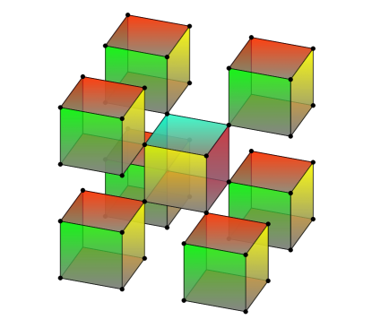
Figure 1: Cutaway diagram showing a decomposition of the cubic lattice into edge-disjoint induced subgraphs, the colored unit cube cells. A cell in the right foreground is omitted for clarity. The collection of vertices specifying each colored cube is defined as $\mathcal{C}$. Under a periodic boundary, each spin appears in exactly two subgraphs. Ising subproblems with $J_{ij}\in\{-1,1\}$, i.e., requiring a single bit of precision, are specified for the cells such that one of each subproblem’s ground states is consistent with its neighbors’. Over the full problem, the concatenation of these partial states forms the planted solution. As discussed in the text, the unit cell Hamiltonians’ lack of shared edges is a crucial property enabling large, tunable changes in complexity while guaranteeing a known ground state.

While the task of creating such problems is of theoretical interest due to their potential assistance in answering open questions about the nature of spin glasses, the pace of research has been hastened in recent years by practical motivations, in particular, the availability of quantum annealing Johnson et al. (2011); Kadowaki and Nishimori (1998) and related analog devices (e.g., optical Wang et al. (2013)) physically implementing Ising Hamiltonian minimization heuristics. Such Hamiltonians are usually constrained by device manufacturing considerations to having short-ranged interaction terms Choi (2008); while more general objectives can typically be encoded onto their native graphs, this may require many system variables for each objective function variable, limiting the problem sizes that can be studied. Hence, a way of encoding topology-native problems is desirable.

In this work, we present a methodology for generating short-range Ising problems with a known ground state. Our primary focus is on the three-dimensional lattice with periodic boundary conditions, primarily because the three-dimensional spin glass is a prototypical complex system and of tremendous interest to condensed matter physicists, but also because the regular structure over the lattice allows a description of our key contributions in a natural and transparent manner. We stress, however, that the method is adaptable to different graph topologies.

By carefully decomposing the underlying graphical structure and selecting Ising subproblems over the resultant components, whose spin-spin interactions are restricted to being bimodal, from classes designed to have specific features influencing hardness, we obtain a factor graph representation having the topology of a body-centered cubic lattice (see Fig. 1). Following a Voronoi tessellation of this lattice, we note that the resultant problem is equivalent to a specific type of three-dimensional tile matching puzzle, a generalization of the two-dimensional edge-matching puzzle Demaine and Demaine (2007). In their two-dimensional form, these puzzles are constraint-satisfaction problems requiring placement of tiles from a given set in permissible spatial locations so that patterns on the tile edges match those of their neighbors. A well-known example is Eternity II ete , a to date unsolved problem for whose solution a $2 million prize was once offered; the prize deadline expired in 2010. Our construction yields polyhedral rather than square puzzle pieces; in particular the units are truncated octahedra whose facets are of various color patterns (see Fig. 6 below). By varying the pattern properties via manipulation of the underlying Ising subproblems, we quickly and efficiently induce a tremendous variation in problem difficulty observed over all examined heuristic algorithms; hundreds of problems at any hardness level within our attainable range can be obtained in seconds with modest computing resources. Hard problems within our class are observed to be many orders of magnitude more difficult than randomly generated spin-glass problems with bimodal disorder, i.e., where the spin-spin interactions are randomly drawn from $\{\pm 1\}$. Despite our restriction to using problem parameters in $\{\pm 1\}$, we can directly generate problems with a known solution that are vastly more difficult than the Gaussian spin glass, which is itself known to be considerably harder than the random bimodal class. We thus consider our construction technique as giving rise to as yet unencountered types of disordered system and discuss our results within the context of hardness phase transitions for combinatorial problems.

The paper is structured as follows. In Sec. II we present an overview of recently-introduced planting techniques, followed by an outline of the planting approach presented in this work in Sec. III. Sections IV and V discuss the relationship of the presented problems to constraint satisfaction problems. Section VI presents numerical experiments using different algorithms highlighting the tunability of typical computational complexity for the problems with planted solutions, followed by discussions, generalizations to other graphs, and concluding remarks.

II Related Work

Our methodology addresses several shortcomings of recently proposed techniques for solution planting in short-range Ising models. In Ref. Hen et al. (2015), a construction method was presented in which frustrated loops with known solution were employed as subproblem units. While the idea is appealing, the resultant problems typically have coupler strengths spanning a large range, posing serious issues for physical devices with precision limitations. An ad hoc limited-precision variant was introduced in Ref. King et al. (2015). Both approaches, however, bear the more serious and systematic disadvantage of tending to generate sets of problems whose members are not of sufficient hardness; we contend that this is a consequence of adding subproblem couplers. It is not hard to see that when partial Hamiltonians having consistent ground states are added, couplers in common which in the individual minima are either both satisfied or both violated will increase in magnitude. In a ground state, however, satisfied couplers are more common than violated ones, hence for any given shared coupler, it is relatively likely that the resultant (added) coupler tends to more strongly prefer alignment with the shared ground state. When this occurs over many edges, the problem’s degrees of freedom are “softly” constrained. The effect is the introduction of “hints” facilitating an optimization algorithm’s task.

In Ref. Marshall et al. (2016), a method was presented for generating difficult instances with bimodal couplers by iteratively changing the couplers’ signs to maximize the time required by a given solver to reach the (hypothesized) ground state. This is a promising approach as it both avoids the coupler addition issue and makes modest precision demands; however, it generally does not allow the ground state to be known with certainty and hence is difficult to scale to larger systems. Furthermore, the approach requires a Monte Carlo-like bond moving algorithm that will likely not easily scale up to much larger problem sizes. The authors do discuss a variant enabling solution planting, but as it again relies on adding couplers, the precision issue returns and, they report, the gains in hardness are modest compared to the mode not controlling the ground state. While the authors provide a useful analysis of post hoc empirical correlates of hardness, for example the parallel tempering mixing time, first proposed in Ref. Yucesoy et al. (2013), the generation procedure is ultimately a local search technique with respect to solver computational time, and hence does not yield or use physical or algorithmic insight at the problem level about what tunes difficulty. In other words, one could not, merely by reference to the resultant Hamiltonian, predict whether the problem is easy or hard. Finally, to design problems based on the time to solution of a given solver, assuming this will carry over to other optimization techniques requires theoretical backing that is missing to date.

A recent paper Wang et al. (2017) introduced the method of patch planting, in which subgraphs with known solution are coupled to each other, satisfying all interactions and thus planting an overall ground state. An advantage is that low-precision and tunable problems can be readily created for a given application domain. The authors report, however, that the resultant problems are observed to be less difficult than random problems, simply because frustrated loops typically do not extend beyond the subgraph building blocks, making the ground state less frustrated than in the fully random case. This problem can be slightly alleviated by post processing mining of the data Wang et al. (2017).

III Problem Construction

Consider a cubic lattice of linear size $L$ with periodic boundary conditions. Let the underlying graph be $G=(V,E)$ with $V$ and $E$ its vertex and edge sets, respectively. Define $U$ to be the vertices of $V$ whose coordinates $(i_{x},i_{y},i_{z})$ consist of integers of the same parity, for example, $(1,3,1)$ or $(0,2,4)$. For each $u\in U$, define $C$ to be the vertices of the cubic unit cell implied when $u$ is opposite to the vertex with coordinates $(i_{x}+1,i_{y}+1,i_{z}+1)$, where the addition is modulo $L$ to account for the periodic boundary. Let $\mathcal{C}$ be the collection of all such cell vertex sets. This construction is partially illustrated in Fig. 1, where each colored unit cell represents a subgraph $G[C]$ induced by a vertex set $C\in\mathcal{C}$ as defined. It should be clear that first, each vertex in $V$ appears in two and only two unit cells and second, that the unit cell subgraphs do not share any edges. In graph terminology, the family $\mathcal{C}$ partitions $G$ into edge-disjoint induced subgraphs.

We are concerned here with constructing Ising problems on the lattice with zero field, i.e., whose Hamiltonians are of the form

$$H({\boldsymbol{s}})=\sum_{ij\in E}J_{ij}s_{i}s_{j}.$$ (1)

Due to the disjointness of the cell edge sets, we can regroup the Hamiltonian into terms each dependent only on the couplings within a unit cell in $\mathcal{C}$,

$$H({\boldsymbol{s}})=\sum_{C\in\mathcal{C}}H_{C}({\boldsymbol{s}}),$$ (2)

where

$$H_{C}({\boldsymbol{s}})\triangleq\sum_{ij\in E[C]}J_{ij}s_{i}s_{j}.$$ (3)

The terms $\{H_{C}({\boldsymbol{s}})\}$ are called the unit cell subproblem Hamiltonians. Specifying each subproblem’s Hamiltonian is sufficient to imply a full Hamiltonian over the lattice. A straightforward consequence of the relation between summation and minimization, exploited in Ref. Hen et al. (2015), is that if the subproblems share the same minimizing configuration ${\boldsymbol{s}}^{*}$, then $H$ is also minimized at ${\boldsymbol{s}}^{*}$. This in turn suggests a natural construction procedure for a problem $H$ with a known ground state. We note a seemingly small but in fact deep and far-reaching difference between prior methodologies and what we propose is that subproblem couplers are never added, avoiding the issue discussed in Sec. II.

It may appear surprising at first that any interesting behavior can result from linking such apparently simple unit-cell subproblems, but this impression turns out to be quite false. Indeed, by restricting our attention to simple classes of subproblems whose couplers belong to the set $\{\pm 1\}$, in other words, representable with a single bit of precision, we can effect dramatic changes in problem complexity, from trivial to many orders of magnitude harder than, e.g., Gaussian spin glasses.

Without loss of generality, we focus on planting the ferromagnetic ground state, i.e., ${\boldsymbol{s}}^{*}=(+1,+1,\ldots,+1)$ and its ${\mathbb{Z}}_{2}$ image, because once such a problem has been generated, the structure of the construction procedure can be concealed by gauge randomization from a would-be adversary seeking the solution. Specifically, to translate to an arbitrarily chosen ground state ${\boldsymbol{t}}^{*}$, one would transform the initially determined couplings $\{J_{ij}\}$ via

$$J^{\prime}_{ij}\leftarrow J_{ij}t_{i}^{*}t_{j}^{*}.$$ (4)

We thus turn our attention to the set of unit-cell Hamiltonians having couplers of magnitude $1$ and ground state ${\boldsymbol{s}}^{*}$. Here we disregard the trivial subproblem comprised uniquely of ferromagnetic bonds; those remaining can be naturally partitioned into three types according to their number of frustrated facets. We call these types $F_{2}$, $F_{4}$, and $F_{6}$, as they contain unit cells with two, four, and six frustrated facets, respectively. These types can be further partitioned into members equivalent under action of the cube graph automorphism group. More precisely, problems within a given equivalence class can be arrived at from one another via transformation from $O_{h}$, the $48$ octahedral symmetries comprised of rotation and reflection leaving a (generic) cube invariant. It turns out that $F_{2}$ and $F_{4}$ contain two such classes (the orbits of $O_{h}$ acting on $F_{2}$ and $F_{4}$, called $F_{21},F_{22}$ and $F_{41},F_{42}$) while all members of $F_{6}$ are equivalent under $O_{h}$. Figure 2 illustrates an arbitrarily-chosen set of equivalence class representatives for the three problems types, while in Figure 3, a few members of type $F_{6}$ are shown.

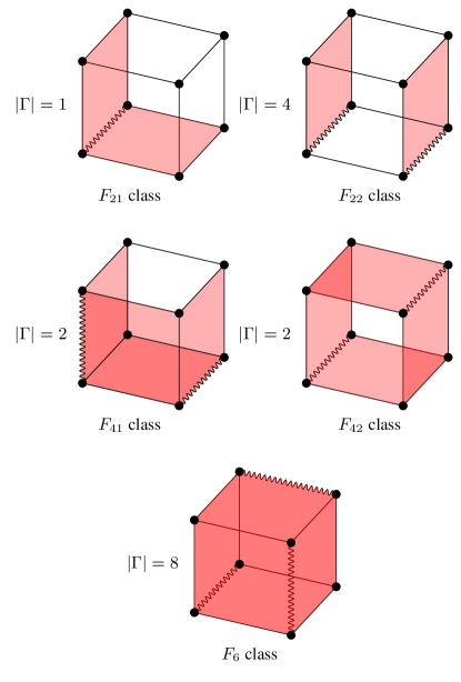
Figure 2: Class representatives of the three unit cell problem types grouped by the number of frustrated facets (shaded). Straight and wavy edges denote ferromagnetic and antiferromagnetic bonds, respectively. All problems have, generally among others, the ferromagnetic state ${\boldsymbol{s}}^{*}=(+1,+1,\ldots,+1)$ as a Hamiltonian minimizer. The total number of ground states $|\Gamma|$ (up to ${\mathbb{Z}}_{2}$ symmetry) for problems within each class is indicated beside each representative.

Figure 3: Selected members of class $F_{6}$, equivalent under octahedral symmetry, that is, one of the $48$ compositions of rotation and reflection leaving an unmarked cube invariant.

Figure 4: All subproblem ground states for a member of class $F_{22}$ (up to ${\mathbb{Z}}_{2}$ symmetry) where black (dark) and red (light) represent spins of opposite sign.

While the subproblems can all readily be verified to have ${\boldsymbol{s}}^{*}$ as a ground state, they clearly differ in the number of other minimizers they possess. Up to ${\mathbb{Z}}_{2}$ symmetry, members of $F_{21}$ have a unique ground state while those of $F_{22}$ have four. All problems in $F_{4}$ and $F_{6}$ have two and eight global minima, respectively. Figure 4 shows the four ground states of a specific member of $F_{22}$. As we will see, this variation in subproblem ground-state degeneracy turns out to exert a crucial effect on the computational difficulty of the final planted problem.

We are now ready to straightforwardly specify our problem construction procedure. First, a probability distribution is chosen over the problem classes $\{F_{ij}\}$. A naive example, which in fact turns out to be a poor choice for generating hard problems, is to sample them uniformly. Next, a distribution over members of the classes is specified. In our examples this was always uniform. The randomness in generating the problems is thus decomposed into what we call subproblem disorder (over the classes) and $O_{h}$ disorder (over the members), the latter so called because it arises equivalently by sampling symmetries of the octahedral group. Subproblems over the unit-cell set $\mathcal{C}$ are then sampled from the defined distributions.

Note that $O_{h}$ disorder is sufficient to induce considerable richness in the types of final problems, even when the cells in $\mathcal{C}$ are all assigned from the same subproblem class. For example, it may appear at first that restricting all subproblems to the class $F_{6}$ (a regime which turns out to be highly interesting) will result in a so-called fully frustrated model Villain (1977), i.e., where all chordless cycles (or plaquettes) are frustrated in the final Hamiltonian, because problems in $F_{6}$ are themselves fully frustrated. That, however, would be incorrect; it is easy to check that cycles forming the facets of unit cubes not in $\mathcal{C}$ may or may not be frustrated depending on the random orientation of the bounding $\mathcal{C}$-cell problems.

It should be pointed out that while the method does ensure that the planted state is in fact a ground state, as the couplers are selected from the $\{\pm 1\}$ class, it is in principle possible for other ground states to exist com (a). Our experimental validation in Sec. VI is thus concerned with the difficulty of finding any ground state. Methods of removing the degeneracy are certainly conceivable and are discussed briefly in Sec. VII.

We proceed next to a further exploration of the problem structure, discussing its connection to tiling puzzles.

IV The puzzle of spin glasses

The proposed problem generation formalism enables translation to a specific type of geometrically appealing constraint-satisfaction problem (CSP) called a tiling puzzle. While these problems are usually defined over two-dimensional domains, we will see that our three-dimensional technique yields a polyhedral generalization of an edge-matching puzzle, an example of which is Eternity II ete . The idea is to abstract the Ising problem into a generic CSP representation known as a factor graph Kschischang et al. (2001). While the Ising Hamiltonian itself can always be interpreted as a factor graph, under our planting technique additional structure is present, namely, the restriction to certain subsets of states. Following construction of the CSP exploiting this structure, the natural connection to a tiling puzzle is observed.

Figure 5 illustrates the necessary steps for the mapping. For clarity, a direct two-dimensional analog of the three-dimensional case is shown, in which the unit cells induced by the decomposition into $\mathcal{C}$ are the cycles forming a checkerboard pattern rather than unit cubes as displayed in Fig. 1.

We first consider the construction of a graph with respect to $\mathcal{C}$, which we call the subproblem lattice, denoted by $\widetilde{G}$. Suppose a vertex is placed at the centroid of each unit cell. The subproblem lattice is defined by considering two such vertices to be adjacent if and only if their corresponding unit cells share a corner vertex. Clearly, this lattice may be $2$-colored, that is, partitioned into two subsets, none of whose members are neighbors. This in turn implies a partitioning of the cells in $\mathcal{C}$ into two disjoint sets $\mathcal{W}$ and $\mathcal{B}$, whose elements are labeled with colors $W$ and $B$, respectively. Figure 5(a) demonstrates the two-dimensional construction of $\widetilde{G}$ and its vertex coloring, where yellow (light shading) and blue (dark shading) may represent labels $W$ and $B$ or vice versa. In three space dimensions, each yellow (light shading) cell is surrounded by eight blue (dark shading) cells instead of four.

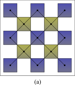
Figure 5: Steps in the derivation of a tile-matching puzzle from the unit-cell planting methodology, shown in two dimensions with a free boundary for clarity. Note that the two-dimensional cells induced by the decomposition are the unit cycle (plaquette) subgraphs arranged in a checkerboard pattern rather than the unit cubes shown in Fig. 1 in three dimensions. (a) The subproblem lattice $\widetilde{G}$ is constructed by placing a vertex at each subproblem cell’s centroid. As discussed in the text, the vertices are 2-colored to yield a convenient representation of the puzzle. In three space dimensions, each yellow (light shading) unit cell contacts eight rather than four blue (dark shading) neighbors; the corresponding $\widetilde{G}$ is the body-centered cubic lattice. (b) Factor graph associated with $\widetilde{G}$, with factors shown as squares. Each vertex is involved in eight factors in three space dimensions. A Voronoi tessellation of $\widetilde{G}$ yields the set of tiling locations. In two space dimensions, these are the areas within the thick lines in panel (c). The factor graph domains, determined by the Ising subproblems, specify a set of allowable tile patterns at each location. The figure shows a hypothetical tile placed at each site. The factor constraints require adjacent colors to agree; hence, the central tile shown has one violation among its four neighbors. The puzzle for the three-dimensional tessellation is shown in Fig. 6.

We next construct the factor graph CSP representation equivalent to the problem of minimizing $H$. The idea is to derive an objective consisting of independent variables subject to equality constraints along the edges of $\widetilde{G}$. First, each vertex in $\widetilde{G}$, mapping to cell $C$ in the original lattice, is identified with a variable ${\boldsymbol{s}}_{C}^{W}$ or ${\boldsymbol{s}}_{C}^{B}$, over eight Ising variables (four in two space dimensions) depending on its label in the $2$-coloring. Because each vertex of the initial lattice is a shared corner of two unit cells in $\mathcal{C}$ of opposite color, in the concatenation of the states $\prod_{C\in\mathcal{W}}{\boldsymbol{s}}_{C}^{W}\prod_{C^{\prime}\in\mathcal{B}}{\boldsymbol{s}}_{C^{\prime}}^{B}$ variables $s_{i}^{W}$ and $s_{i}^{B}$ will occur exactly once for each vertex $i\in V$. The domain of each subproblem lattice variable is simply the ensemble of its subproblem ground states, the ground-state set $\Gamma_{C}$, so that the full configuration space of the new problem is the Cartesian product

$$\Gamma^{W,B}\triangleq\prod_{C\in\mathcal{W}}\Gamma_{C}\prod_{C^{\prime}\in\mathcal{B}}\Gamma_{C^{\prime}}.$$ (5)

To be a feasible solution to the original problem however, equality of neighboring variables must be enforced, that is, $s_{i}^{W}=s_{i}^{B}$ $\forall$ $i$. If we define the problem

$$\max_{{\boldsymbol{s}}^{W,B}\in\Gamma^{W,B}}\prod_{i\in V}\delta[s_{i}^{W},s_{i}^{B}],$$ (6)

where $\delta(x,y)=1$ if $x=y$ and zero otherwise, we readily see that the solution is obtained for the overall planted ground state ${\boldsymbol{s}}^{B}={\boldsymbol{s}}^{W}={\boldsymbol{s}}^{*}$. To make the graphical connection, we note that each $\delta$ function in Eq. (6) can be interpreted as a factor over neighboring subproblem lattice variables (identified with) $C,C^{\prime}$, i.e., $\psi_{C,C^{\prime}}({\boldsymbol{s}}_{C}^{W},{\boldsymbol{s}}_{C^{\prime}}^{B})\triangleq\delta[s_{i}^{W},s_{i}^{B}]$ with $i=C\cap C^{\prime}$. The final maximization objective is then the product of all factors over subproblem lattice variables

$$f({\boldsymbol{s}}^{W,B})=\prod_{C,C^{\prime}\in\widetilde{E}}\psi_{C,C^{\prime}}({\boldsymbol{s}}^{W},{\boldsymbol{s}}^{B}),$$ (7)

where the product index refers to edges of $\widetilde{G}$ by the cells in $\mathcal{C}$ mapping to their endpoint vertices. The factor graph corresponding to the two-dimensional lattice in Fig. 5 (a) appears in Fig. 5 (b), with variables represented by circular vertices (whose colors identify their labels as $W$ or $B$) and factors by the squares along the edges. In three dimensions, each variable is involved in eight factors rather than four.

Consider now the subproblem lattice with its vertices lying at their “natural” points in Euclidean space, i.e., at the centroids of the unit cells, rather than as a generic graph. A Voronoi tessellation Torquato (2013) is a partitioning of the space surrounding the vertices into convex polytopes, usually called tiles, but for reasons that will soon be clear, we refer to as tiling locations such that all points within a polytope are closest (typically in the $L_{2}$-norm sense) to the enclosed vertex. It is easy to see in Fig. 5(a) that in two dimensions, the subproblem lattice forms a periodic pattern, sometimes called the quincunx, of squares of length $2$, each with a central vertex. The appropriate tessellation of $\widetilde{G}$ is a partitioning into tilted square regions centered at each vertex. Neglecting for an instant the significance of the colors, Fig. 5(c) shows five full and eight partial tiling squares in the section of lattice drawn. Returning to the CSP in which the task was to assign the variables from their respective domains (ground-state sets) so that factor constraints are satisfied, we now observe the equivalence to a tile-matching puzzle. This is comprised of a board (the space embedding $\widetilde{G}$), segmented into octagons (the cells in the Voronoi tessellation), each of which is endowed with a repertoire of tiles (the ground-state set associated with the location). The tile faces could be in one of two colors (the spin values, not to be confused with the $2$-coloring introduced to construct the CSP). The puzzle task is to select the tiles so that no two adjacent tile faces have a different color. If orange (light) and purple (dark) represent spin values, say, $1$ and $-1$, respectively, then Fig. 5 (c) shows a hypothetical tiling assignment. Here a violation occurs where the tile colors on both sides of a factor differ.

Figure 6: Tile-matching puzzle associated with three-dimensional unit-cell planting. The tile locations are truncated octahedra, the elements of a bitruncated cubic honeycomb, and in turn the Voronoi tessellation of the body-centered-cubic lattice $\widetilde{G}$. Color constraints are defined among neighboring hexagonal facets of the octahedra; the square facets are uninvolved. Four of the eight factors associated with a location are shown (the other four point into the page). In the example configuration shown, one constraint satisfaction and two violations occur.

In three dimensions, the puzzle is analogous, but with a few twists. In a generalization of the two-dimensional case, the subproblem lattice $\widetilde{G}$ will, when respecting Euclidean coordinates, form a pattern of cubes of length $2$, each with a vertex at its centroid. Such a formation is known as the body-centered-cubic lattice. The corresponding Voronoi tessellation is the space-filling bitruncated cubic honeycomb whose base unit is the truncated octahedron Conway et al. (2016); Torquato (2013). Each of these polyhedral cells, which now define the three-dimensional tiling locations, consists of eight hexagonal facets, through which the the edges of our CSP factor graph pass, and six square facets, defining the boundaries between $\widetilde{G}$ vertices at distance $2$, but through which no CSP factors pass. The ground-state sets associated with each vertex of $\widetilde{G}$ thus map to coloring configurations on the hexagonal facets of the enclosing Voronoi cell, defining a set of tiles, and again the task is to place the tiles while meeting all coloring constraints. The construction is illustrated in Fig. 6.

While technically fitting the definition of a tile-matching puzzle, the specific examples proposed here differ in a key way from conventional puzzles such as Eternity II. In the latter, each tile from the given set may be placed at more than one board location (in an allowable orientation) while presently the ground-state set associated with each site constrains the choices. This fact, along with the polynomial-time solvability Barahona (1982) of the original ground-state problem in two dimensions, could lead one to suspect that the puzzles we have contrived may not be overly interesting. In three space dimensions, however, solution by graph matching is no longer applicable, and as we will see, the problems exhibit a rich range of behavior intimately tied to the known properties of generic constraint satisfaction problems.

V The phases of satisfaction

Hardness phase transitions in combinatorial problems have been an active area of study for several decades now Hogg et al. (1996). Of particular interest is the emergence of difficulty divergencies in random SAT problems as parameters guiding instance generation are varied Mézard et al. (2002). While the tiling CSPs we have proposed here can certainly be expressed as SAT problems com (b), the resultant formulas do not, however, follow the typical assumptions of random SAT. Most notably, the variables are not free to appear in any clause with some probability, but follow the highly structured topological constraints of the puzzle. Of course, the subproblem and $O_{h}$ disorder impose stochasticity over the factor graph variable domains $\{\Gamma_{C}\}$, but this is a localized randomness, violating key assumptions in the analysis of random SAT. Nonetheless, we expect that commonly known facts and intuitions regarding the relation between how constrained a problem is and its empirical hardness will apply to our situation.

Because the tiling puzzle color factors are invariant to the distribution over cell problems, constrainedness depends exclusively on the features of the ground-state sets. As we alluded to earlier, a dominant correlate of problem hardness is the average size of the ground-state sets $\mathbb{E}|\Gamma|$. A highly constrained regime is one in which the subproblems tend to have relatively small degeneracy and vice versa for a loosely constrained one. A subproblem demonstrating a maximal constraint level is any member of class $F_{21}$ (with a unique ground state up to ${\mathbb{Z}}_{2}$), while one constrained minimally, which was not considered in the experiments, is the zero $J$ subproblem, in which all $256$ states are ground states. Within the class of subproblems introduced in Sec. III, including members of $F_{21}$ and $F_{6}$ (with degeneracy $8$) tends to bias the final problem towards the maximal and minimal extremes, respectively.

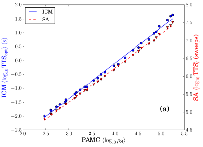
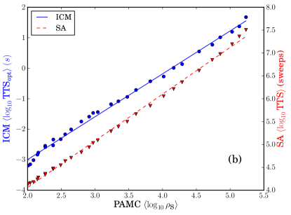
Figure 7: Simulated annealing $\langle\log_{10}{\rm TTS}\rangle$ (right $y$-axes, red triangles) and parallel tempering with isoenergetic cluster moves $\langle\log_{10}{\rm TTS}_{\textrm{opt}}\rangle$ (left $y$-axes, blue circles) as a function of population annealing Monte Carlo $\langle\log_{10}\rho_{\rm S}\rangle$ for three-dimensional problem classes (a) gallus_26 and (b) gallus_46. The SA and ICM ${\rm TTS}$ are measured in Monte Carlo sweeps and seconds, respectively. Within each problem class, every point in a given color (symbol) jointly shows the two corresponding measures for one of the $30$ subclasses described in the text (averages are computed over $200$ instances from each subclass). The data show that PAMC $\langle\log\rho_{\rm S}\rangle$ exhibits a strong linear correlation with the other two algorithms’ $\log{\rm TTS}$ metrics, confirming its power as a measure of hardness and landscape roughness. Furthermore, as relative hardness measures for these problems, the three quantities studied here can be used more or less interchangeably. Error bars have been omitted for clarity.

By construction, all our problems are satisfiable, i.e., there is no unsatisfiable (or overconstrained) regime as usually understood. Clearly, the minimally constrained full problem is trivial as each state is a solution to the original problem. In the tiling puzzle representation, the factor constraints can be met independently because the resultant states are always in the ground-state sets. At the other extreme, highly constrained problems are also typically easy: Because there are few local choices from the ground-state sets, a tree search method will encounter relatively small branching factors when traversing the state space, while for local search, the energy landscape will be such that the algorithm can reliably locate the ground state using simple strategies to escape from local minima. These extremes strongly suggest that for some intermediate level of mean ground-state set size, a peak in problem hardness will occur. While it is not possible to increase $|\Gamma_{C}|$ past $8$ for unit cells without introducing more complex Ising interactions (or without trivially removing all $J_{ij}$), an interesting question, probed experimentally in the following, is, given the proposed classes of unit-cell subproblems ($F_{2}$, $F_{4}$, and $F_{6}$) and all possible mixture distributions over the classes, did the hypothesized peak occur for some interior point of the distribution set? An affirmative answer would suggest that the corresponding CSP class is among the hardest of all tile-matching puzzles of the type we have introduced, i.e., for which the locations’ tile sets may be chosen arbitrarily, not by constraining them to map to subproblem ground states. Conversely, if the hardness maximum within the set of mixtures occurs at the set boundary, it would point to the existence of more difficult tiling puzzles not representable within our framework.

VI Experiments

We now numerically study the typical complexity of certain subproblem classes to illustrate their tunability. This section focuses on three-dimensional cubic lattices, followed by a demonstration that the approach works well also in two space dimensions (Sec. VII.2). We conclude with a discussion of generalizations to other graph types.

While we would ideally have performed a rigorous numerical study for a discrete “grid” representing all subproblem types we have proposed, this is computationally prohibitive. Consequently, we focus on two illustrative regimes demonstrating interesting variations in problem difficulty over three algorithms, and the role played by subproblem degeneracy. The simulation results show that highly complex problems with known ground state, and more difficult than conventional spin glasses with both Gaussian and random bimodal couplings, are accessible via our methodology, but they also strongly suggest that the hardness maximum over the distribution set occurs at a boundary, namely, when the distribution is a point mass concentrated on class $F_{6}$. Perhaps unsurprisingly then, we conclude that tiling puzzles equivalent to Ising problems constructed using the classes $\{F_{2},F_{4},F_{6}\}$ are likely not the hardest among those where the tile sets are arbitrarily specifiable.

All problems are defined on three-dimensional lattices of size $8\times 8\times 8$ with periodic boundary conditions. We consider two classes of problems corresponding to one-dimensional slices of the problem mixture parameter space. The first class, gallus_26, allows subproblems to belong solely to classes $F_{6}$ and $F_{22}$, while in the second, gallus_46, they are constrained to $F_{6}$ and $F_{42}$. Both instance classes are parametrized by $p_{6}$, the probability of selecting class $F_{6}$ instead of the alternative com (c). The classes each contained $200$ instances generated at $30$ uniformly spaced values of $p_{6}\in[0.8,1]$, for a total of $6000$ instances per class. All subproblems are subject to uniform $O_{h}$ disorder. The selected range of $p_{6}$ values is interesting as within it, problems are more difficult than conventional spin glasses with Gaussian or random bimodal couplings. We note that the problems continue to become easier as $p_{6}$ decreases. Using the values of $|\Gamma|$ shown in Fig. 2, the expected ground-state set sizes in terms of $p_{6}$ are $\mathbb{E}|\Gamma|=8p_{6}+4(1-p_{6})$ for gallus_26 and $\mathbb{E}|\Gamma|=8p_{6}+2(1-p_{6})$ for gallus_46.

Figure 8: Average log-entropic family size $\langle\log_{10}\rho_{\rm S}\rangle$ (population annealing Monte Carlo landscape roughness measure) for $L=8$ cubic lattice classes gallus_26 and gallus_46. Each point corresponds to a subclass in which unit-cell subproblems are selected from $F_{6}$ with probability $p_{6}$, or else from $F_{22}$ for gallus_26 and from $F_{24}$ for gallus_46. Averages are computed over $200$ instances from each subclass. Plots of (a) $\langle\log_{10}\rho_{\rm S}\rangle$ against $p_{6}$ and (b) $\langle\log_{10}\rho_{\rm S}\rangle$ against $\mathbb{E}|\Gamma|$, the expected subproblem degeneracy within their range of overlap. For a given mixing probability $p_{6}$, (a) shows that gallus_26 is consistently more difficult than gallus_46 despite being less frustrated. On the other hand, (b) shows that instances from either class with a given subproblem degeneracy have very similar difficulty, suggesting that $\mathbb{E}|\Gamma|$ considerably explains the variation in hardness irrespective of the specific underlying subproblem mixture or frustration level. In light of the proposed tiling puzzle interpretation, this is consistent with knowledge of CSP hardness. For reference, note the $\langle\log_{10}\rho_{\rm S}\rangle$ values of equal-sized spin glasses with random $\pm 1$ and Gaussian interactions. For certain subclasses, the problems proposed here are far more difficult than the traditionally used cases.

Problem difficulty is assessed through performance of three different algorithms designed for problems with rough energy landscapes. The measures of difficulty are in strong agreement across the methods, providing corroboration that the observed difficulty trends should persist robustly across a fairly large class of heuristic algorithms, including backtrack-based search Hogg et al. (1996).

Simulated annealing (SA) Kirkpatrick et al. (1983) is the most basic algorithm considered. We use the optimized implementation developed by Isakov et al. Isakov et al. (2015) with $\beta_{\min}=0.01$ and $\beta_{\max}=1$. While we would rather have used some form of optimized time to solution (TTS) measure, which considers the best tradeoff between simulation length and number of simulations, SA runs were too time consuming on the hard problems to generate the requisite runtime histograms reliably. Consequently, we selected a fixed run length of $N_{S}=8192$ sweeps for all problems with a single sweep per temperature. Each problem is simulated $R=10^{6}$ times independently. The SA TTS is defined as the computational time required to find a ground state with at least $99$% probability, i.e., for each instance, ${\rm TTS}=N_{S}\log(0.01)/\log(1-p)$, where $p$ is the fraction of successful runs out of the $R$ repetitions.

Furthermore, we have used a highly optimized implementation of parallel tempering Monte Carlo with isoenergetic cluster moves (ICMs) Zhu et al. (2015), an adaptive hybrid parallel tempering (PT) Hukushima and Nemoto (1996); Geyer (1991); Moreno et al. (2003) cluster algorithm Houdayer (2001). Because the ICM is considerably more efficient than SA, it allowed us to gather runtime statistics for each instance, allowing optimized ${\rm TTS}$s to be computed. In contrast to SA, total ICM computational time is not merely a function of overall Monte Carlo sweeps, but includes the additional cost of constructing random-sized clusters. Consequently, to track aggregated ICM computational effort we record run times in seconds on hardware dedicated entirely to the simulations. If $P(\tau)$ is the empirically observed probability of finding the ground state in time $\tau$ or less, the optimized time to solution is defined as ${\rm TTS}_{\textrm{opt}}=\min_{\tau}\tau\log(0.01)/\log[1-P(\tau)]$. We note, however, that despite the efficiency of the ICM, it commonly failed to find the solution for the harder problems within the maximum allowed $2^{24}$ total Monte Carlo sweeps, requiring $60-75$ min of real time, when computing the runtime histograms. For difficult classes, these “timeouts” occurred at least half of the time within the $100$ ICM repetitions used to tally the histograms. Fortunately, we were nonetheless able to infer an optimized ${\rm TTS}$ from the conditional histogram in which solutions were found. We used $N_{T}=30$ temperatures spaced within $T_{\max}=3$ and $T_{\min}=0.01$; see Ref. Zhu et al. (2015) for further details of the ICM.

The final set of tests have used the sequential Monte Carlo Del Moral et al. (2006) method known as population annealing Monte Carlo (PAMC) Hukushima and Iba (2003); Machta (2010). This algorithm is related to SA but differs crucially in its usage of weight-based resampling, which multiplies or eliminates members of a population according to the ratios of their Boltzmann factors at adjacent temperatures, maintaining thermal equilibrium at each step. Our simulations used $N_{T}=201$ temperatures with $1/T=\beta\in[0.0,5]$ and $N_{s}=10$ sweeps per temperature, and a population size of $R=5\times 10^{5}$ replicas. In Ref. Wang et al. (2015a), a PAMC-derived index of landscape roughness called the entropic family size $\rho_{\rm S}$ was proposed. If $q_{i}$ is the fraction of replicas in the final population descended from initial replica $i$, then $\rho_{\rm S}=\lim_{R\to\infty}R/e^{h[q]}$, where $h[q]=-\sum_{i}q_{i}\log q_{i}$. An energy landscape is thus deemed rough if $h[q]$ is small, that is, if relatively few initial replicas survive to the final distribution, yielding a large value of $\rho_{\rm S}$. Note that $\rho_{\rm S}$ converges quickly in $R$ and is easily estimated with finite populations. Thermal equilibration is ensured by requiring $h[q]>\log 100$; when this is not satisfied for an instance, it is rerun with a larger population size. The entropic family size $\rho_{\rm S}$ is known to covary strongly with the PT autocorrelation time Wang et al. (2015a) and, as can be seen from Fig. 7, does so for the ${\rm TTS}$-based hardness metrics considered here as well. Figure 7 shows, respectively, the dependence of both SA and ICM $\langle\log_{10}{\rm TTS}\rangle$ measures on PAMC $\langle\log_{10}\rho_{\rm S}\rangle$ for the $30$ subclasses of gallus_26 [Fig. 7(a)] and gallus_46 [Fig. 7(b)] studied, where the averages $\langle\cdots\rangle$ at each point representing a subclass are computed over its $200$ generated instances. The plots clearly show a distinct near-linear dependence of both time-based measures on the PAMC-defined value. A larger $\rho_{\rm S}$ on average implies a longer time to solution with respect to both SA and ICM algorithms, corroborating the former’s power as an objective measure of landscape roughness.

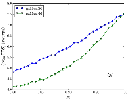
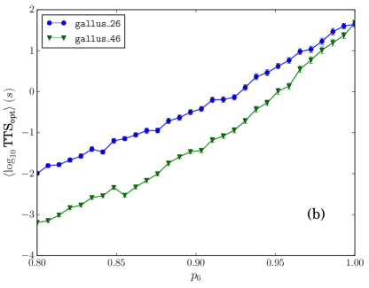
Figure 9: (a) SA $\langle\log_{10}{\rm TTS}\rangle$ and (b) ICM $\langle\log_{10}{\rm TTS}_{\textrm{opt}}\rangle$ (b) plotted against the parameter $p_{6}$ for $30$ subclasses of gallus_26 and gallus_46 defined in the text. The problems show the same relative difficulty trends with respect to both algorithms and in accordance with the PAMC results shown in Fig. 8 (a).

Results of the PAMC simulations are shown in Fig. 8. We observe a trend of increasing $\rho_{\rm S}$ (and hence complexity) for both problem classes as the fraction of subproblems from $F_{6}$ increases towards unity. For comparison, we display the mean $\log\rho_{\rm S}$ value of two prototypical problems with rough landscapes on the same lattice, the random $J_{ij}\in\{\pm 1\}$ and Gaussian $J_{ij}\sim N(0,1)$ [$N(0,1)$ a normal distribution with zero mean and variance one] spin glass, computed using $1000$ and $5099$ instances of each type, respectively. It is clear that problems in most of the examined subclasses of gallus_26 and gallus_46 are more difficult than both of these widely studied problem classes. Indeed, for subclasses of gallus_26 corresponding to $p_{6}\in[0.91,1]$, problems are $\sim 2-3$ orders of magnitude harder than bimodal spin glasses. Perhaps more surprisingly, they are also $\sim 2-3$ orders more difficult than Gaussian spin glasses, despite the latter possessing continuous-valued couplings while our instances restrict couplers to $\{\pm 1\}$, which are believed to generally be easier to minimize.

Setting $p_{6}=1$ yields the most complex problems of those considered. In fact, we conjecture, based on less comprehensive simulations, that these instances are the hardest among all those constructed with subproblem classes in $\{F_{2},F_{4},F_{6}\}$. We plan to perform a comprehensive analysis in the future. For this hard class, the unit-cell subproblems, deriving exclusively from $F_{6}$, have eight ground states each. Because this hardness peak occurs at the boundary of the problem parameter space, it seems plausible that one could instantiate yet more complex three-dimensional tiling puzzles, where the locations were allowed more than eight (times two) tile possibilities but not so many that the problem becomes underconstrained and easy to solve.

At first, the greater pointwise difficulty shown in Fig. 8 of an $\{F_{6},F_{22}\}$ mixture over one made of $\{F_{6},F_{42}\}$ appears to contradict intuition that greater frustration implies higher difficulty. After all, with four bounding frustrated facets, a member of $F_{42}$ can be interpreted as more frustrated than one of $F_{22}$, which has two. The story is somewhat more subtle though: While frustration certainly plays a role in tuning hardness in our problems, it appears to do so through its effect on constraint level, namely, on the sizes of $\Gamma_{C}$, with $F_{22}$ inducing higher complexity than $F_{42}$ because its ground-state set size is larger. This fact is displayed in Fig. 8(b), where $\log\rho_{\rm S}$ for the two classes is plotted against $\mathbb{E}|\Gamma|$ instead of $p_{6}$. The graph shows that for a given value of $\mathbb{E}|\Gamma|$, gallus_26 and gallus_46 have a very similar roughness index, implying that mean subproblem degeneracy accurately predicts difficulty regardless of the underlying subproblem mixture.

For completeness, analogous plots displaying similar difficulty trends for SAs $\log{\rm TTS}$ and ICMs $\log{\rm TTS}_{\textrm{opt}}$ are shown in Fig. 9, where they are again plotted against $p_{6}$.

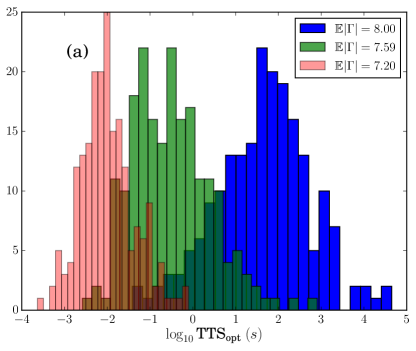
Figure 10: Histograms of (optimized) $\log_{10}{\rm TTS}_{\textrm{opt}}$ relative to isoenergetic cluster moves for classes (a) gallus_26 and (b) gallus_46 for three subclasses characterized here by mean subproblem degeneracy $\mathbb{E}|\Gamma|$; $200$ problems within each subclass were used to obtain the histograms. The leftward trend in both sets of histograms shows clearly that the problems become easier with decreasing $\mathbb{E}|\Gamma|$ and their shapes suggest that ${\rm TTS}_{\textrm{opt}}$ is log-normally distributed.

In contrast to our results so far, which have considered instance-averaged difficulty measures, Fig. 10 shows histograms of optimized ICM $\log_{10}{\rm TTS}$ values for three subclasses of gallus_26 [Fig. 10(a)] and of gallus_46 [Fig. 10(b)] indexed by $\mathbb{E}|\Gamma|$. The leftward shift in histogram support shows clearly that problems tend to become easier with decreasing $\mathbb{E}|\Gamma|$. Given the histogram shapes, one may naturally suspect that ${\rm TTS}_{\textrm{opt}}$ is log-normally distributed. As $\log{\rm TTS}$ is unlikely to be precisely normal across the entire data range, we visualize correspondence with a Gaussian via normal probability plots Chambers et al. (1983), which relate the sample order statistics, obtained by sorting the data, with the theoretical means of the corresponding normal order statistics. Deviations from a linear relation signal lack of Gaussianity. Figure 11 shows the probability plots for the three subclasses used to generate the preceding histograms for the gallus_26 [Fig. 11(a)] and gallus_46 [Fig. 11(b)] classes, respectively. The relation is close to linear over the majority of the histogram support, implying in turn that the ${\rm TTS}_{\textrm{opt}}$ is approximately log-normally distributed. This is consistent with quantities such as the parallel tempering Monte Carlo autocorrelation time and other roughness measures Katzgraber et al. (2006); Yucesoy et al. (2013) having the same property.

While we have argued that $\mathbb{E}|\Gamma|$ is a good predictor of mean difficulty, the histogram results show that this value by no means provides a complete picture. Indeed, when $\mathbb{E}|\Gamma|=8$ (i.e., $p_{6}=1$) there is no variance in $|\Gamma_{C}|$ as all subproblems have eight-fold degeneracy, yet the $\log{\rm TTS}$ distributions in Fig. 10 nonetheless show considerable intraclass spread in difficulty. Therefore, there are certainly other factors at play in predicating the hardness.

Figure 11: Normal probability plots of ICMs $\log_{10}{\rm TTS}_{\textrm{opt}}$ for the instance subclasses used to generate the histograms in Fig. 10. A linear relation between the Gaussian theoretical and data quantiles implies that the data follow a normal distribution. The plots show clearly that for the three representative subclasses of (a) gallus_26 and (b) gallus_46 parametrized by $\mathbb{E}|\Gamma|$, the histograms are close to normal over the majority of their support. In other words, ${\rm TTS}_{\textrm{opt}}$ approximately follows a log-normal distribution.

VII Discussion

In this section we discuss generalizations of the planting approach using lattice animals. Furthermore, we present a case study on how the approach generalizes to other non hypercubic lattices. Finally, we discuss the use of the planted problems for fundamental studies of spin glasses and related statistical systems.

VII.1 Generalization via lattice animals

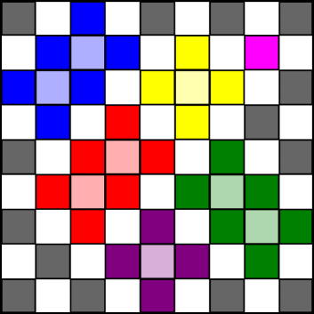
Figure 12: Generalization of unit-cell planting using lattice animals, also known as polyominoes. Illustrations are in two dimensions for clarity. The analogous procedure in three space dimensions is similar. With lattice animal planting, the edge-disjoint subgraphs underlying the subproblems are no longer restricted to the unit cells in $\mathcal{C}$ (the checkerboard in two space dimensions and the decomposition in Fig. 1 for three space dimensions) but are now permitted to be connected subgraphs comprised of unions of cells from $\mathcal{C}$. As before, subproblem couplers are not added. Above, six such subgraphs in non gray colors are shown, of which only the pink one (top right) is comprised of a single cell. If the tree widths of the lattice animals are small, their ground states can be computed exactly and gauged to the overall target ground state. This extension considerably expands types of subproblems that can be employed and also introduces an additional mechanism of solution hiding via randomization of the employed lattice animals.

The proposed unit-cell planting technique shows encouraging results and properties and one may inquire how it may be generalized. In this section, we present a natural extension of the idea, still assuming lattice-structured problems, where instead of defining subproblems on the unit cells of $\mathcal{C}$, they are specified on subgraphs consisting of their unions. One can verify that such subgraphs, called lattice animals or polyominoes, also partition the lattice into edge-disjoint subgraphs, meaning that subproblem couplers are still not added.

A two-dimensional example of decomposition into lattice animals is shown in Fig. 12. Generalization to three-dimensional polyominoes obtained by grouping cells from the decomposition shown in Fig. 1 is straightforward. Shown in non-gray colors are six lattice animals. Only the pink (top right) one is made of a single cell. The key difference from the basic method is that unit cells of a given color are no longer constrained to have their individual ground states agree; only the complete animal ground state is relevant. This extension thus considerably extends the types of subproblems that can be employed and also introduces an additional mechanism of solution hiding, namely, via randomization of the employed lattice animals, which would of course be unknown to the would-be adversary. While the tiling puzzle and CSP interpretation of the problem, suitably modified, continues to hold in this generalization, under lattice animal randomization, the adversary would in essence no longer be certain what puzzle they are even solving.

In this work, we have considered carefully chosen families of subproblems on three-dimensional unit cells. An exploration of extensions to more general lattice animals is outside the scope of the present work. We note, however, that if subproblem couplers are sampled from a given distribution, then provided the subgraph tree widths are small, their ground states can be computed exactly Koller and Friedman (2009) and gauged to the desired overall ground state.

Finally, we note that this lattice animal generalization is also key when attempting to reduce degeneracy in the planted problems. For example, by selecting the coupler values from a Sidon set Sidon (1932); Katzgraber et al. (2015); Karimi et al. (2017) of the form $\{\pm(n-2)/n,\pm(n-1)/n,\pm 1\}$ with, e.g., $n=50$, the degeneracy is drastically reduced. Similarly, one could select the couplers from a distribution of the form

$$|J_{ij}|\in a+(1-a)u,$$ (8)

where $u\in[0,1)$ is a uniform random number and $a$ close to $1$ Katzgraber (2010). However, instead of using basic tiles, more complex lattice animals must be used to construct the problems.

VII.2 Generalization to arbitrary graphs

The need to benchmark both classical and quantum optimization heuristics has hastened the development of advanced planting techniques for solutions of spin-glass-like optimization problems. We have so far focused our attention on hypercubic lattice problems. However, quantum annealing machines typically have hardwired hardware graphs that are close to planar. A prototypical example is the chimera graph Bunyk et al. (2014) used by current versions of the D-wave quantum annealing machines. When presented with such a situation, one has two possible options to apply our planting framework. The first is to impose a lattice structure onto the available graph and the second is to specify subproblems on altogether different “unit cells” than cubes, which of course, must be graph dependent. We now discuss the first option applied to the special case of chimera.

Figure 13: Implementation of a $6\times 6$ square lattice with periodic (toroidal) boundary from a $3\times 3$ unit-cell chimera graph. (a) Instantiation of two-dimensional logical spins from the chimera. For concreteness, $36$ lattice spins are assumed to be labeled in row-fastest order. First, each spin in the bipartite cells is paired with the directly opposing spin of the same cell. Next, the resultant spin pairs, called dimers, are forced to behave as one spin via strong ferromagnetic coupling. Each dimer is labeled with the corresponding lattice logical spin. (b) In the first and last columns of cells, lattice problem edges between dimers $\{1,2\}$ and $\{3,4\}$ of each cell are added. Note that only one of the two existing cell edges is shown, but if both are used, the coupler strength must be suitably divided. (c) In the top and bottom rows of cells, lattice edges between dimers $\{1,3\}$ and $\{2,4\}$ of each cell are added. Again, only one of the two available edges is displayed. (d) All inter cell couplers are specified according to the lattice problem. The lattice variables are labeled beside each dimer again, from which one can verify that the resultant construction does indeed implement a $6\times 6$ two-dimensional torus.

Although in principle three-dimensional lattices can be implemented on the chimera graph Harris et al. (2017), the required overhead may limit linear (planted) problem sizes that can be practically studied. On the other hand, relatively large two-dimensional lattices with periodic boundaries can be straightforwardly embedded on chimera, with a relatively modest constant ratio of two chimera variables per lattice spin. More precisely, a chimera graph of $L\times L$ bipartite unit cells, comprised of $8L^{2}$ variables in total, can produce a toroidal two-dimensional lattice of size $2L\times 2L$. Rather than formally describe the rather natural procedure, we illustrate it in Fig. 13, where a $6\times 6$ periodic lattice is created from a $3\times 3$ $K_{4,4}$ cell chimera graph.

So far, we have focused primarily on planting subproblems on three-dimensional unit cells, in part because planar problems without a field are solvable in polynomial time Barahona (1982), but as illustrated in Figs. 5 and 12, the two-dimensional analog is readily obtained. The analytical tractability of the planar lattice enables a deep exploration of physical and computational properties, a work which will be reported elsewhere Perera et al. (2018). Here we outline the idea and demonstrate that it does indeed perform well on planar lattices and nonplanar quasi-two-dimensional chimera graphs using population annealing simulations. The two-dimensional subproblems, i.e., the analogs of the cells shown in Fig. 2, are partitioned into classes $\{C_{i}\}$ for $i\in\{1,\ldots,4\}$, within which cells have $i$ minimizing ground-state configurations each. To achieve the construction, first define two magnitudes $J_{s},J_{l}>0$ with $J_{l}>J_{s}$; presently we take $J_{l}=2$ and $J_{s}=1$. A cell in class $C_{i}$ is constructed by setting a random edge to be antiferromagnetic with magnitude $J_{s}$, $i-1$ of the remaining edges to be ferromagnetic with magnitude $J_{s}$, and the leftover edges to be ferromagnetic with magnitude $J_{l}$ com (d). It is readily verified that the subproblems do indeed have the specified number of local ground states which always include the ferromagnetic state.

Figure 14: Average log-entropic family size $\langle\log_{10}\rho_{\rm S}\rangle$ for $L=24$ periodic planar lattice classes C_23 and C_24. Each point corresponds to a subclass in which unit cell subproblems are selected from $C_{2}$ with probability $p_{2}$, or else from $C_{3}$ for C_23 and from $C_{4}$ for C_24. Averages are computed over $200$ instances from each subclass. As for the study in three dimensions, we see a large range of landscape roughness, again with a range of subclasses demonstrating greater difficulty than equal-sized random bimodal spin-glass problems. The most difficult problems in our ensemble are those in which the subproblems are exclusively selected from $C_{2}$, in which the local GS degeneracy is $2$.

As was done in three space dimensions, we consider two classes of problems each comprised of mixtures of two subproblem classes. Problem class C_24, consists of mixtures of $C_{2}$ and $C_{4}$ cells, while in C_23 the cells may belong to $C_{2}$ or $C_{3}$. Both problem classes are parametrized by $p_{2}$, the probability of choosing a cell from $C_{2}$. The results on $24\times 24$ periodic lattices are shown in Fig.  14. Again, a wide range of landscape roughness is seen to be attainable, including a regime in which the problems are more difficult than random bimodal ($\pm 1$ couplers) spin glasses. An interesting distinction from three-dimensional results is that the most difficult problems are not those in which cells exclusively belong to the maximally degenerate class $C_{4}$, but rather the moderately constrained $C_{2}$ class. In fact, class $C_{4}$ is a highly underconstrained regime for this topology and gives rise to very easy problems. The fascinating connections between dimension, complexity, and phase behavior are the subject of ongoing study that goes beyond the scope of this paper.

If one wished to move beyond a regular lattice structure, the natural objective is a decomposition of the problem graph $G$ into edge-disjoint subgraphs satisfying some constraint allowing tractable minimization. An example of a constrained decomposition is into subgraphs with given minimum vertex degree Yuster (2013). More directly applicable to the planting context would be a constraint on maximum subgraph tree width thereby allowing determination of the planted subproblem ground states. The edge-disjointness property is the key common aspect with the ideas presented in this paper, as it continues to circumvent the need for adding subproblem couplers. This idea is clearly a generalization of the lattice animal methodology discussed previously. While we have not presently considered planting using such generic subgraphs, one can readily envision a heuristic decomposition algorithm that greedily grows partitioning subgraphs until their tree widths exceed some criterion.

VII.3 Spin-glass physics

We hope researchers in the field embrace these planted problems to study physical properties of glassy systems beyond the benchmarking of optimization heuristics.

Having arbitrarily large planted solutions for hypercubic lattices allows one to address different problems in the physics of spin glasses. For example, the computation of defect energies, intimately related to fundamental properties of these paradigmatic disordered systems, strongly depends on the knowledge of ground states (see, for example, Refs. Hartmann (1997, 1999); Palassini and Young (1999, 2001); Hartmann (2001); Katzgraber et al. (2001)). Being able to plant problems would drastically reduce the computational effort in answering these fundamental questions.

Furthermore, by carefully tuning the different instance classes, problems with different disorder and frustration can be generated. A systematic study of the interplay between disorder and frustration is therefore possible for nontrivial lattices beyond hierarchical ones. Similarly, being able to tune the fraction of frustrated plaquettes allows one to carefully study the emergence of chaotic effects in spin glasses (see, for example, Refs. Katzgraber and Krzakala (2007); Thomas et al. (2011); Wang et al. (2015b) and references therein).

VII.4 Application-based benchmark problems

It is well established that random benchmark problems Rønnow et al. (2014); Katzgraber et al. (2014) for classical and quantum solvers using spin-glass-like problems are computationally typically easy. Furthermore, the control over the hardness of the benchmark problems has been rather limited either because (post) processing is expensive Katzgraber et al. (2015); Marshall et al. (2016) or because the benchmark generation approach does not give the user enough control over the problems to match, e.g., hardware restrictions Hen et al. (2015).

Because application-based problems from industrial settings are highly structured, they pose additional challenges for the vast pool of optimization techniques designed, in general, for random unstructured problems. This has sparked the use of problems from industry to generate hard (and sometimes tunable) benchmark problems. Most notably, the use of circuit fault diagnosis Perdomo-Ortiz et al. (2015); Perdomo-Ortiz et al. has produced superbly hard benchmarks with small number of variables. However, the use of application-based problems for benchmarking is in its infancy and while circuit fault diagnosis shows most promise Perdomo-Ortiz et al. , many applications have produced benchmark problems that lack the richness needed to perform systematic studies; see, for example, Refs. Perdomo-Ortiz et al. (2012); Santra et al. (2014); Rieffel et al. (2015); Azinovic et al. (2017).

The problems presented in this work are highly tunable and computationally easy to generate. Furthermore, they can be embedded in more complex graphs, as is, for example, commonly done on the D-wave hardware for application benchmarks. Thus, having this tunability not only should allow for the generation of problems that might elucidate quantum speedup in analog annealers, but might also help gain a deeper understanding into quantum annealing for spin glasses in general. In parallel, having these tunable problems might elucidate the application scope of specific optimization techniques, both classical and quantum.

VIII Conclusions

We have presented an approach for generating Ising Hamiltonians with planted ground-state solutions and a tunable complexity based on a decomposition of the model graph into edge-disjoint subgraphs. Although we have performed the construction for three-dimensional cubic lattices and illustrated the approach with the two-dimensional pendant, the approach can be generalized to other lattice structures, as shown in Sec. VII.2 for the chimera lattice. The construction allows for a wide range in computational complexity depending on the mix of the elementary building blocks used. We corroborated these results with experiments using different optimization heuristics. Subsequent studies should discuss constructions with controllable ground-state degeneracy, as well as the mapping of the complete complexity phase space.

References

- Bach (1983) E. Bach, in Proceedings of the fifteenth annual ACM Symposium on Theory of Computing (ACM, 1983).
- Pilcher and Rardin (1987) M. G. Pilcher and R. L. Rardin, A random cut generator for symmetric traveling salesman problems with known optimal solutions, Institute for Interdisciplinary Engineering Studies, Purdue University Lafayette, IN, Tech. Rep. CC-87-4 (1987).
- Pilcher and Rardin (1992) M. G. Pilcher and R. L. Rardin, Partial polyhedral description and generation of discrete optimization problems with known optima, Naval Research Logistics (NRL) 39, 839 (1992).
- Barthel et al. (2002) W. Barthel, A. K. Hartmann, M. Leone, F. Ricci-Tersenghi, M. Weigt, and R. Zecchina, Hiding solutions in random satisfiability problems: A statistical mechanics approach, Phys. Rev. Lett. 88, 188701 (2002).
- Monasson and Zecchina (1996) R. Monasson and R. Zecchina, Entropy of the K-satisfiability problem, Phys. Rev. Lett. 76, 3881 (1996).
- Johnson et al. (2011) M. W. Johnson, M. H. S. Amin, S. Gildert, T. Lanting, F. Hamze, N. Dickson, R. Harris, A. J. Berkley, J. Johansson, P. Bunyk, et al., Quantum annealing with manufactured spins, Nature 473, 194 (2011).
- Kadowaki and Nishimori (1998) T. Kadowaki and H. Nishimori, Quantum annealing in the transverse Ising model, Phys. Rev. E 58, 5355 (1998).
- Wang et al. (2013) Z. Wang, A. Marandi, K. Wen, R. L. Byer, and Y. Yamamoto, Coherent Ising machine based on degenerate optical parametric oscillators, Phys. Rev. A 88, 063853 (2013).
- Choi (2008) V. Choi, Minor-embedding in adiabatic quantum computation. I: The parameter setting problem., Quantum Inf. Process. 7, 193 (2008).
- Demaine and Demaine (2007) E. D. Demaine and M. L. Demaine, Jigsaw puzzles, edge matching, and polyomino packing: Connections and complexity, Graphs and Combinatorics 23, 195 (2007).
- (11) Eternity II puzzle, accessed 19 May 2017, URL https://goo.gl/n3VvsX.
- Hen et al. (2015) I. Hen, J. Job, T. Albash, T. F. Rønnow, M. Troyer, and D. A. Lidar, Probing for quantum speedup in spin-glass problems with planted solutions, Phys. Rev. A 92, 042325 (2015).
- King et al. (2015) A. D. King, T. Lanting, and R. Harris, Performance of a quantum annealer on range-limited constraint satisfaction problems (2015), arXiv:1502.02098.
- Marshall et al. (2016) J. Marshall, V. Martin-Mayor, and I. Hen, Practical engineering of hard spin-glass instances, Phys. Rev. A 94, 012320 (2016).
- Yucesoy et al. (2013) B. Yucesoy, J. Machta, and H. G. Katzgraber, Correlations between the dynamics of parallel tempering and the free-energy landscape in spin glasses, Phys. Rev. E 87, 012104 (2013).
- Wang et al. (2017) W. Wang, S. Mandrà, and H. G. Katzgraber, Patch-planting spin-glass solution for benchmarking, Phys. Rev. E 96, 023312 (2017).
- Villain (1977) J. Villain, Spin glass with non-random interactions, J. Phys. C 10, 1717 (1977).
- com (a) Referring to the subproblem classes though, a few moments’ reflection reveals that interestingly, free spin degeneracy is impossible in the planted state.
- Kschischang et al. (2001) F. R. Kschischang, B. J. Frey, and H.-A. Loeliger, Factor graphs and the sum-product algorithm, IEEE Transactions on information theory 47, 498 (2001).
- Torquato (2013) S. Torquato, Random heterogeneous materials: microstructure and macroscopic properties (Springer Science & Business Media, Berlin, 2013).
- Conway et al. (2016) J. H. Conway, H. Burgiel, and C. Goodman-Strauss, The symmetries of things (CRC Press, London, 2016).
- Barahona (1982) F. Barahona, On the computational complexity of Ising spin glass models, J. Phys. A 15, 3241 (1982).
- Hogg et al. (1996) T. Hogg, B. A. Huberman, and C. P. Williams, Phase transitions and the search problem (Elsevier, Amsterdam, 1996).
- Mézard et al. (2002) M. Mézard, G. Parisi, and R. Zecchina, Analytic and Algorithmic Solution of Random Satisfiability Problems, Science 297, 812 (2002).
- com (b) If factor graph domain values and are mapped to Boolean values, say, and , respectively, the color constraints are clearly xor functions and their conjunction must be part of the Boolean formula. To obtain a conjunctive normal form (CNF) expression, a naive way to incorporate the ground sets is to straightforwardly represent each variable’s in disjunctive normal form, convert it to CNF, and include it in the formula by conjunction. The expression size is likely highly suboptimal but, for our case, nonetheless polynomially bounded and illustrates the point.
- com (c) Hence, when , the classes are identical.
- Kirkpatrick et al. (1983) S. Kirkpatrick, C. D. Gelatt, Jr., and M. P. Vecchi, Optimization by simulated annealing, Science 220, 671 (1983).
- Isakov et al. (2015) S. V. Isakov, I. N. Zintchenko, T. F. Rønnow, and M. Troyer, Optimized simulated annealing for Ising spin glasses, Comput. Phys. Commun. 192, 265 (2015), (see also ancillary material to arxiv:cond-mat/1401.1084).
- Zhu et al. (2015) Z. Zhu, A. J. Ochoa, and H. G. Katzgraber, Efficient Cluster Algorithm for Spin Glasses in Any Space Dimension, Phys. Rev. Lett. 115, 077201 (2015).
- Hukushima and Nemoto (1996) K. Hukushima and K. Nemoto, Exchange Monte Carlo method and application to spin glass simulations, J. Phys. Soc. Jpn. 65, 1604 (1996).
- Geyer (1991) C. Geyer, in 23rd Symposium on the Interface, edited by E. M. Keramidas (Interface Foundation, Fairfax Station, VA, 1991), p. 156.
- Moreno et al. (2003) J. J. Moreno, H. G. Katzgraber, and A. K. Hartmann, Finding low-temperature states with parallel tempering, simulated annealing and simple Monte Carlo, Int. J. Mod. Phys. C 14, 285 (2003).
- Houdayer (2001) J. Houdayer, A cluster Monte Carlo algorithm for 2-dimensional spin glasses, Eur. Phys. J. B. 22, 479 (2001).
- Del Moral et al. (2006) P. Del Moral, A. Doucet, and A. Jasra, Sequential monte carlo samplers, Journal of the Royal Statistical Society: Series B (Statistical Methodology) 68, 411 (2006).
- Hukushima and Iba (2003) K. Hukushima and Y. Iba, in The Monte Carlo method in the physical sciences: celebrating the 50th anniversary of the Metropolis algorithm, edited by J. E. Gubernatis (AIP, 2003), vol. 690, p. 200.
- Machta (2010) J. Machta, Population annealing with weighted averages: A Monte Carlo method for rough free-energy landscapes, Phys. Rev. E 82, 026704 (2010).
- Wang et al. (2015a) W. Wang, J. Machta, and H. G. Katzgraber, Population annealing: Theory and application in spin glasses, Phys. Rev. E 92, 063307 (2015a).
- Chambers et al. (1983) J. M. Chambers, W. S. Cleveland, B. Kleiner, and P. A. Tukey, Graphical methods for data analysis, vol. 5 (Wadsworth, Belmont, CA, 1983).
- Katzgraber et al. (2006) H. G. Katzgraber, S. Trebst, D. A. Huse, and M. Troyer, Feedback-optimized parallel tempering Monte Carlo, J. Stat. Mech. P03018 (2006).
- Koller and Friedman (2009) D. Koller and N. Friedman, Probabilistic graphical models: principles and techniques (MIT press, Cambridge, MA, 2009).
- Sidon (1932) S. Sidon, Ein Satz über trigonometrische Polynome und seine Anwendung in der Theorie der Fourier-Reihen, Mathematische Annalen 106, 536 (1932).
- Katzgraber et al. (2015) H. G. Katzgraber, F. Hamze, Z. Zhu, A. J. Ochoa, and H. Munoz-Bauza, Seeking Quantum Speedup Through Spin Glasses: The Good, the Bad, and the Ugly, Phys. Rev. X 5, 031026 (2015).
- Karimi et al. (2017) H. Karimi, G. Rosenberg, and H. G. Katzgraber, Effective optimization using sample persistence: A case study on quantum annealers and various Monte Carlo optimization methods, Phys. Rev. E 96, 043312 (2017).
- Katzgraber (2010) H. G. Katzgraber, Random Numbers in Scientific Computing: An Introduction (2010), (arXiv:1005.4117).
- Bunyk et al. (2014) P. Bunyk, E. Hoskinson, M. W. Johnson, E. Tolkacheva, F. Altomare, A. J. Berkley, R. Harris, J. P. Hilton, T. Lanting, and J. Whittaker, Architectural Considerations in the Design of a Superconducting Quantum Annealing Processor, IEEE Trans. Appl. Supercond. 24, 1 (2014).
- Harris et al. (2017) R. Harris et al., in preparation (2017).
- Perera et al. (2018) D. Perera, F. Hamze, and H. G. Katzgraber, in preparation (2018).
- com (d) Hence two bits of precision are required for these classes.
- Yuster (2013) R. Yuster, Edge-disjoint induced subgraphs with given minimum degree, The Electronic Journal of Combinatorics 20, P53 (2013).
- Hartmann (1997) A. Hartmann, Evidence for nontrivial ground-state structure of 3d spin glasses, Europhys. Lett. 40, 429 (1997).
- Hartmann (1999) A. K. Hartmann, Scaling of stiffness energy for three-dimensional Ising spin glasses, Phys. Rev. E 59, 84 (1999).
- Palassini and Young (1999) M. Palassini and A. P. Young, Triviality of the ground state structure in Ising spin glasses, Phys. Rev. Lett. 83, 5126 (1999).
- Palassini and Young (2001) M. Palassini and A. P. Young, The spin glass: Effects of ground state degeneracy, Phys. Rev. B 63, 140408(R) (2001).
- Hartmann (2001) A. K. Hartmann, Ground-state clusters of two-, three-, and four-dimensional Ising spin glasses, Phys. Rev. E 63 (2001).
- Katzgraber et al. (2001) H. G. Katzgraber, M. Palassini, and A. P. Young, Monte Carlo simulations of spin glasses at low temperatures, Phys. Rev. B 63, 184422 (2001).
- Katzgraber and Krzakala (2007) H. G. Katzgraber and F. Krzakala, Temperature and Disorder Chaos in Three-Dimensional Ising Spin Glasses, Phys. Rev. Lett. 98, 017201 (2007).
- Thomas et al. (2011) C. K. Thomas, D. A. Huse, and A. A. Middleton, Chaos and universality in two-dimensional Ising spin glasses, Phys. Rev. Lett. 107, 047203 (2011).
- Wang et al. (2015b) W. Wang, J. Machta, and H. G. Katzgraber, Chaos in spin glasses revealed through thermal boundary conditions, Phys. Rev. B 92, 094410 (2015b).
- Rønnow et al. (2014) T. F. Rønnow, Z. Wang, J. Job, S. Boixo, S. V. Isakov, D. Wecker, J. M. Martinis, D. A. Lidar, and M. Troyer, Defining and detecting quantum speedup, Science 345, 420 (2014).
- Katzgraber et al. (2014) H. G. Katzgraber, F. Hamze, and R. S. Andrist, Glassy Chimeras Could Be Blind to Quantum Speedup: Designing Better Benchmarks for Quantum Annealing Machines, Phys. Rev. X 4, 021008 (2014).
- Perdomo-Ortiz et al. (2015) A. Perdomo-Ortiz, B. O’Gorman, J. Fluegemann, R. Biswas, and V. N. Smelyanskiy, Determination and correction of persistent biases in quantum annealers (2015), (arXiv:quant-phys/1503.05679).
- (62) A. Perdomo-Ortiz, A. Feldman, A. Ozaeta, S. V. Isakov, Z. Zhu, B. O’Gorman, H. G. Katzgraber, A. Diedrich, H. Neven, J. de Kleer, et al., On the readiness of quantum optimization machines for industrial applications, (unpublished).
- Perdomo-Ortiz et al. (2012) A. Perdomo-Ortiz, N. Dickson, M. Drew-Brook, G. Rose, and A. Aspuru-Guzik, Finding low-energy conformations of lattice protein models by quantum annealing, Sci. Rep. 2, 571 (2012).
- Santra et al. (2014) S. Santra, G. Quiroz, G. Ver Steeg, and D. A. Lidar, Max 2-SAT with up to 108 qubits, New J. Phys. 16, 045006 (2014).
- Rieffel et al. (2015) E. G. Rieffel, D. Venturelli, B. O’Gorman, M. B. Do, E. M. Prystay, and V. N. Smelyanskiy, A case study in programming a quantum annealer for hard operational planning problems, Quant. Inf. Proc. 14, 1 (2015).
- Azinovic et al. (2017) M. Azinovic, D. Herr, B. Heim, E. Brown, and M. Troyer, Assessment of Quantum Annealing for the Construction of Satisfiability Filters, SciPost Phys. 2, 013 (2017).