Maximizing Algebraic Connectivity of Constrained Graphs in Adversarial Environments

Abstract

This paper aims to maximize algebraic connectivity of networks via topology design under the presence of constraints and an adversary. We are concerned with three problems. First, we formulate the concave-maximization topology design problem of adding edges to an initial graph, which introduces a nonconvex binary decision variable, in addition to subjugation to general convex constraints on the feasible edge set. Unlike previous approaches, our method is justifiably not greedy and is capable of accommodating these additional constraints. We also study a scenario in which a coordinator must selectively protect edges of the network from a chance of failure due to a physical disturbance or adversarial attack. The coordinator needs to strategically respond to the adversary’s action without presupposed knowledge of the adversary’s feasible attack actions. We propose three heuristic algorithms for the coordinator to accomplish the objective and identify worst-case preventive solutions. Each algorithm is shown to be effective in simulation and their compared performance is discussed.

I Introduction

Motivation. Multi-agent systems are pervasive in new technology spaces such as power networks with distributed energy resources like solar and wind, mobile sensor networks, and large-scale distribution systems. In such systems, communication amongst agents is paramount to the propagation of information, which often lends itself to robustness and stability of the system. Network connectivity is well studied from a graph-theoretic standpoint, but the problem of designing topologies when confronted by engineering constraints or adversarial attacks is not well addressed by current works. We are motivated to study the NP-hard graph design problem of adding edges to an initial topology and to develop a method to solve it which has both improved performance and allows for direct application to the aforementioned constrained and adversarial settings.

Literature Review. The classic paper [7] by Miroslav Fiedler proposes a scalar metric for the algebraic connectivity of undirected graphs, which is given by the second-smallest eigenvalue of the graph Laplacian and is also referred to as the Fiedler eigenvalue. One of the main problems we are interested in studying is posed in [8], where the authors develop a heuristic for strategically adding edges to an initial topology to maximize this eigenvalue. Lower and upper bounds for the Fiedler eigenvalue with respect to adding a particular edge are found; however, the work is limited in that their approach is greedy and may not perform well in some cases. In addition, the proposed strategy does not address how to handle additional constraints that may be imposed on the network, such as limits on nodal degree or restricting costlier edges. The authors of [1] aim to solve the problem of maximizing connectivity for a particular robotic network scenario in the presence of an adversarial jammer, although the work does not sufficiently address scenarios with a more general adversary who may not be subject to dynamical constraints. The Fiedler eigenvector, which has a close relationship to the topology design problem, is studied in [11]. Many methods to compute this eigenvector exist, such as the cascadic method in [12]. However, these papers do not fully characterize how this eigenvector evolves from adding or removing edges from the network, which is largely unanswered by the literature. The authors of [6] study the spectra of randomized graph Laplacians, and [13] gives a means to estimate and maximize the Fiedler eigenvalue in a mobile sensor network setting. However, neither of these works consider the problem from a design perspective. In the celebrated paper by Goemans and Williamson [10], the authors develop a relaxation and performance guarantee on solving the MAXCUT problem, which has not yet been adapted for solving the topology design problem. Each of [5, 2] survey existing results related to the Fiedler eigenvalue and contain useful references.

Statement of Contributions. This paper considers three optimization problems and has two main contributions. First, we formulate the concave-maximization topology design problem from the perspective of adding edges to an initial network, subject to general convex constraints plus an intrinsic binary constraint. We then pose a scenario where a coordinator must strategically select links to protect from random failures due to a physical disturbance or malicious attack by a strategic adversary. In addition, we formulate this problem from the adversary’s perspective. Our first main contribution is a method to solve the topology design problem (and, by extension, the protected links problem). We develop a novel MAXCUT-inspired SDP relaxation to handle the binary constraint, which elegantly considers the whole problem in a manner where previous greedy methods fall short. Our next main contribution returns to the coordinator-adversary scenario. We first discuss the nonexistence of a Nash equilibrium in general. This motivates the development of an optimal preventive strategy in which the coordinator makes an optimal play with respect to any possible response by the adversary. We rigorously prove several auxiliary results about the solutions of the adversary’s computationally hard concave-minimization problem in order to justify heuristic algorithms which may be used by the coordinator to search for the optimal preventive strategy. A desirable quality of these algorithms is they do not presuppose the knowledge of the adversary’s feasibility set, nor the capability of solving her problem. Rather, the latter two algorithms observe her plays over time and use these against her construct an effective preventive solution. Simulations demonstrate the effectiveness of our SDP relaxation for topology design and the performance of the preventive-solution seeking algorithms when applied to the adversarial link-protection problem.

II Preliminaries

This section establishes some notation and preliminary concepts which will be drawn upon throughout the paper.

II-A Notation

We denote by $\operatorname{\mathbbm{R}}$ the set of real numbers. The notation $x\in\operatorname{\mathbbm{R}}^{n}$ and $A\in\operatorname{\mathbbm{R}}^{n\times m}$ indicates an $n$-dimensional real vector and an $n$-by-$m$-dimensional real matrix, respectively. The gradient of a real-valued multivariate function $f:\operatorname{\mathbbm{R}}^{n}\rightarrow\operatorname{\mathbbm{R}}$ with respect to a vector $x\in\operatorname{\mathbbm{R}}^{n}$ is written $\nabla_{x}f(x)$. The $i^{\textup{th}}$ component of a vector $x$ is indicated by $x_{i}$, all components of $x$ not including the $i^{\textup{th}}$ component is indicated by $x_{-i}$, and the $(i,j)^{\textup{th}}$ element of a matrix $A$ is indicated by $A_{ij}$. The standard inner product is written $\left\langle x,y\right\rangle=x^{\top}y$ and the Euclidean norm of a vector $x$ is denoted $\|x\|_{2}=\sqrt{\langle x,x\rangle}$. The closed Euclidean ball of radius $\varepsilon$ centered at a point $x$ is expressed as $\mathcal{B}_{\varepsilon}(x)$. Two vectors $x$ and $y$ are perpendicular if $\left\langle x,y\right\rangle=0$, indicated by $x\perp y$, and the orthogonal complement to a span of vectors $a_{i}$ is written $\operatorname{span}\{a_{i}\}^{\perp}$, meaning $x\perp y,\forall x\in\operatorname{span}\{a_{i}\},\forall y\in\operatorname{span}\{a_{i}\}^{\perp}$. Elementwise multiplication is represented by $x\diamond y=(x_{1}y_{1},\dots,x_{n}y_{n})^{\top}$. A symmetric matrix $A\in\operatorname{\mathbbm{R}}^{n\times n}$ has $n$ real eigenvalues ordered as $\lambda_{1}\leq\dots\leq\lambda_{n}$, sometimes written $\lambda_{i}(A)$ if clarification is needed, with associated eigenvectors $v_{1},\dots,v_{n}$ that are assumed to be of unit magnitude unless stated otherwise. A positive semi-definite matrix $A$ is indicated by $A\succeq 0$. We denote componentwise inequality as $x\succeq y$. The notation $\operatorname{\mathbf{0}}_{n}$ and $\operatorname{\mathbf{1}}_{n}$ refers to the $n$-dimensional vectors of all zeros and all ones, respectively. We use the notation $\operatorname{\mathbbm{I}}_{n}:=I_{n}-\dfrac{\mathbf{1}_{n}\mathbf{1}^{\top}_{n}}{n}$ and refer to this matrix as a pseudo-identity matrix; note that $\operatorname{null}{(\operatorname{\mathbbm{I}}_{n})}=\operatorname{span}\{\operatorname{\mathbf{1}}_{n}\}$. The operator $\operatorname{diag}$ for vector arguments produces a diagonal matrix whose diagonal elements are the entries of the vector. The empty set is denoted $\emptyset$ and the cardinality of a finite set $\mathcal{S}$ is denoted $|\mathcal{S}|$. We express the $m$ Cartesian product of sets by means of a superscript $m$, such as $[\underline{s}_{i},\overline{s}_{i}]^{m}\subset\operatorname{\mathbbm{R}}^{m}$, where $\underline{s}_{i},\overline{s}_{i}\in\operatorname{\mathbbm{R}}$. Probabilities and expectations are indicated by $\operatorname{\mathbbm{P}}$ and $\operatorname{\mathbbm{E}}$, respectively.

II-B Graph Theory

We refer to [9] as a supplement for the concepts we describe throughout this subsection. In multi-agent engineering applications, it is useful to represent a network mathematically as a graph $\operatorname{\mathcal{G}}=(\operatorname{\mathcal{N}},\operatorname{\mathcal{E}})$ whose node set is given by $\operatorname{\mathcal{N}}=\{1,\dots,n\}$ and edge set $\operatorname{\mathcal{E}}\subseteq\operatorname{\mathcal{N}}\times\operatorname{\mathcal{N}}$, $|\operatorname{\mathcal{E}}|=m$, which represents a physical connection or ability to transmit a message between agents. We refer to the set of nodes that node $i$ is connected to as its set of neighbors, $\operatorname{\mathcal{N}}_{i}\subset\operatorname{\mathcal{N}}$. We consider undirected graphs so $(i,j)\in\operatorname{\mathcal{E}}$ indicates $j\in\operatorname{\mathcal{N}}_{i}$ and $i\in\operatorname{\mathcal{N}}_{j}$. The graph has an associated Laplacian matrix $L\in\operatorname{\mathbbm{R}}^{n\times n}$, whose elements are

$$L_{ij}=\begin{cases}-1,&j\in\operatorname{\mathcal{N}}_{i},j\neq i,\\ |\operatorname{\mathcal{N}}_{i}|,&j=i,\\ 0,&\text{otherwise}.\end{cases}$$

Note that $L\succeq 0$. It is well known that the multiplicity of the zero eigenvalue is equal to the number of connected components in the graph [9]. To expand on this, connected graphs have a one-dimensional null space associated with the eigenvector $\operatorname{\mathbf{1}}_{n}$. The incidence matrix of $L$ is given by $E\in\{-1,0,1\}^{n\times m}$, where the $l^{\textup{th}}$ column of $E$, given by $e_{l}\in\{-1,0,1\}^{n}$, is associated with an edge $l\sim(i,j)$. In particular, the $i^{\textup{th}}$ element of $e_{l}$ is $-1$, the $j^{\textup{th}}$ element is $1$, and all other elements are zero. A vector $x\in\{0,1\}^{m}$ encodes the (dis)connectivity of the edges. In this sense, for $l\in\{1,\dots,m\}$, $x_{l}=0$ indicates $l$ is disconnected and $x_{l}=1$ indicates $l$ is connected. Then, $L=E\operatorname{diag}(x)E^{\top}$.

II-C Set Theory

A limit point $p$ of a set $\mathop{\mathcal{P}}\nolimits$ is a point such that any neighborhood $\mathcal{B}_{\varepsilon}(p)$ contains a point $p^{\prime}\in\mathop{\mathcal{P}}\nolimits$. A set is closed if it contains all of its limit points, it is bounded if it is contained in a ball of finite radius, and it is compact if it is both closed and bounded. Let $\mathcal{A}_{i}=\{p\;|\;a_{i}^{\top}p\geq b_{i}\}$ be a closed half-space and $\mathop{\mathcal{P}}\nolimits=\mathcal{A}_{1}\cap\dots\cap\mathcal{A}_{r}\subset\operatorname{\mathbbm{R}}^{m}$ be a finite intersection of closed half-spaces. If $\mathop{\mathcal{P}}\nolimits$ is compact, we refer to it as a polytope. Consider a set of points $\mathcal{F}=\{p\in\mathop{\mathcal{P}}\nolimits\;|\;a_{i}^{\top}p=b_{i},i\in\mathcal{I}\subseteq\{1,\dots,r\};a_{j}^{\top}p\geq b_{j},j\in\{1,\dots,r\}\setminus\mathcal{I}\}$. Let $h=\dim(\operatorname{span}\{a_{i}\})$ be the dimension of the subspace spanned by the vectors $\{a_{i}\}_{i\in\mathcal{I}}$. Then, we refer to $\mathcal{F}$ as an $(m-h)$-dimensional face of $\mathop{\mathcal{P}}\nolimits$. Lastly, denote the affine hull of $\mathcal{F}$ as $\operatorname{aff}(\mathcal{F})=\{p+w\;|\;p,w\in\operatorname{\mathbbm{R}}^{m},p\in\mathcal{F},w\perp\operatorname{span}\{a_{i}\}_{i\in\mathcal{I}}\}$ and define the relative interior of $\mathcal{F}$ as $\operatorname{relint}(\mathcal{F})=\{p\;|\;\exists\varepsilon>0:\mathcal{B}_{\varepsilon}(p)\cap\operatorname{aff}(\mathcal{F})\subset\mathcal{F}\}$.

III Problem Statements

This section formulates the three optimization problems that we study. The first problem aims to add edges to an initial topology to maximize algebraic connectivity of the final graph. The second problem introduces a coordinator who is charged with protecting some links in a network that are subject to an external disturbance or attack. The third problem takes the opposite approach of the latter problem by minimizing connectivity from an adversarial point of view.

III-A Topology Design for Adding Edges

Consider a network of agents with some initial (possibly disconnected) graph topology characterized by an edge set $\operatorname{\mathcal{E}}_{0}$ and Laplacian $L_{0}$. We would like to add $k$ edges to $\operatorname{\mathcal{E}}_{0}$, possibly subject to some additional convex constraints, so as to maximize the Fiedler eigenvalue of the final Laplacian $L^{\star}$. This problem is well motivated: the Fiedler eigenvalue dictates convergence rate of many first-order distributed algorithms such as consensus and gradient descent. First, let $\operatorname{\mathcal{E}}$ be the complete edge set (not including redundant edges or self loops) with $m=|\operatorname{\mathcal{E}}|$. Consider the incidence matrix $E$ associated with $\operatorname{\mathcal{E}}$ and the vector of edge connectivities $x$, as described in Section II-B. The constrained topology design problem is then formulated as

$$\operatorname{\mathsf{P}}1:\ \underset{x,\alpha}{\text{max}} \alpha,$$ (1a)

subject to $$E(\operatorname{diag}(x))E^{\top}\succeq\alpha\operatorname{\mathbbm{I}}_{n},$$ (1b)

$$\sum_{l=1}^{m}x_{l}\leq k+|\operatorname{\mathcal{E}}_{0}|,$$ (1c)

$$x\in\operatorname{\mathcal{X}},$$ (1d)

$$x_{l}=1,\ l\sim(i,j)\in\operatorname{\mathcal{E}}_{0},$$ (1e)

$$x_{l}\in\{0,1\},\ l\in\{1,\dots,m\}.$$ (1f)

In $\operatorname{\mathsf{P}}1$, the solution $\alpha^{\star}$ is precisely the value for $\lambda_{2}$ of the final Laplacian solution given by $L(x^{\star})=E(\operatorname{diag}(x^{\star}))E^{\top}$. This is encoded in the constraint (1b), where the pseudo-identity matrix $\operatorname{\mathbbm{I}}_{n}$ has the effect of filtering out the fixed zero-eigenvalue of the Laplacian. A useful relation is $\lambda_{2}=\underset{z}{\text{inf}}\{z^{\top}L(x)z\;|\;z\perp\operatorname{\mathbf{1}}_{n},\|z\|_{2}=1\}$, which shows that $\lambda_{2}$ as a function of $x$ is a pointwise infimum of linear functions of $x$ and is therefore concave. By extension, $\operatorname{\mathsf{P}}1$ is a concave-maximization problem in $x$. The set $\operatorname{\mathcal{X}}$ is assumed compact and convex and may be chosen by the designer in accordance with problem constraints such as bandwidth/memory limitations, restrictions on nodal degrees, or restricting certain edges from being chosen. These constraints may manifest in applications such as communication bandwidth limitations amongst Distributed Energy Resource Providers for Real-Time Optimization in renewable energy dispatch [4]. The binary constraint (1f) is nonconvex and makes the problem NP-hard. Handling this constraint is one of the main objectives of this paper and will be addressed in Section IV.

As for existing methods of solving $\operatorname{\mathsf{P}}1$, one option is solve it over the convex hull of the constraint set, which is given by $[0,1]^{m}\cap\operatorname{\mathcal{X}}$. Then, the problem may be solved in $k$ steps by iteratively adding the edge $l\sim(i,j)$ for which $x_{l}$ is maximal in each step. This is discussed in [8] and the references therein. Although this method allows the designer to easily capture $\operatorname{\mathcal{X}}$, it is not a satisfying relaxation because the underlying characteristics of the connectivity are not well captured. The authors of [8] propose an alternate method which chooses the edge $l$ for which $\dfrac{\partial\lambda_{2}}{\partial x_{l}}=v_{2}^{\top}\dfrac{\partial L(x)}{\partial x_{l}}v_{2}=v_{2}^{\top}e_{l}e_{l}^{\top}v_{2}=(v_{2,i}-v_{2,j})^{2}$ is maximal. This method is limited in that it is (a) greedy and (b) cannot account for $\operatorname{\mathcal{X}}$. We are motivated to develop a relaxation for $\operatorname{\mathsf{P}}1$ which improves on existing techniques in both performance and the capability of handling constraints.

III-B Topology Design for Protecting Edges

We now formulate a problem which is closely related to $\operatorname{\mathsf{P}}1$ and interesting to study in its own right. Motivated by the scenario of guarding against disruptive physical disturbances or adversarial attacks, consider a coordinator who may protect up to $k_{s}$ links from failing in a network. The failure of the links are assumed to be independent Bernoulli random variables whose probabilities are encoded by the vector $p\in[0,1]^{m}$. Then, consider the coordinator’s decision vector $s\in\mathop{\mathcal{S}}\nolimits=\{0,1\}\cap\mathop{\mathcal{S}}\nolimits^{\prime}$, where $\mathop{\mathcal{S}}\nolimits^{\prime}$ is assumed compact and convex. We write out the Laplacian as before, $L(x)=E\operatorname{diag}(x)E^{\top}$. Following a disturbance or attack, the probability that an edge $l$ is (dis)connected is given by $\operatorname{\mathbbm{P}}(x_{l}\equiv 1)=(s_{l}-1)p_{l}+1$ (resp. $\operatorname{\mathbbm{P}}(x_{l}\equiv 0)=(1-s_{l})p_{l}$). The interpretation for the vector $s$ here is that, if a particular element $s_{l}=1$, it is deterministically connected and considered immune to the disturbance or attack. The coordinator’s problem is:

$$\operatorname{\mathsf{P}}2:\ \underset{s,\alpha}{\text{max}} \alpha,$$ (2a)

subject to $$\operatorname{\mathbbm{E}}\left[E(\operatorname{diag}(x))E^{\top}\right]\succeq\alpha\operatorname{\mathbbm{I}}_{n},$$ (2b)

$$\operatorname{\mathbbm{P}}(x_{l}\equiv 1)=(s_{l}-1)p_{l}+1,$$ (2c)

$$\operatorname{\mathbbm{P}}(x_{l}\equiv 0)=(1-s_{l})p_{l},$$ (2d)

$$\sum_{l=1}^{m}s_{l}\leq k_{s},$$ (2e)

$$s\in\mathop{\mathcal{S}}\nolimits,^{\prime}\quad s\in\{0,1\}^{m}.$$ (2f)

Due to the linearity of the expectation operator, (2b) is equivalent to $E(\operatorname{diag}((s-\operatorname{\mathbf{1}}_{m})\diamond p+\operatorname{\mathbf{1}}_{m}))E^{\top}\succeq\alpha\operatorname{\mathbbm{I}}_{n}$, which is an LMI (linear matrix inequality) in $s$. We note that, as in $\operatorname{\mathsf{P}}1$, the objective of $\operatorname{\mathsf{P}}2$ may be thought of as a pointwise infimum of linear functions and, as such, is a binary concave-maximization problem in $s$.

The formulation in $\operatorname{\mathsf{P}}2$ presupposes a fixed vector $p$. However, it may be the case that a strategic attacker detects preventive action taken by the coordinator and adjusts her strategy to improve the likelihood of disconnecting the network. We now formulate the attacker’s problem for some known, fixed coordinator strategy $s$:

$$\operatorname{\mathsf{P}}3:\ \underset{p,\alpha}{\text{min}} \alpha,$$ (3a)

subject to $$\lambda_{2}(\operatorname{\mathbbm{E}}\left[E(\operatorname{diag}(x))E^{\top}\right])=\alpha,$$ (3b)

$$\operatorname{\mathbbm{P}}(x_{l}\equiv 1)=(s_{l}-1)p_{l}+1,$$ (3c)

$$\operatorname{\mathbbm{P}}(x_{l}\equiv 0)=(1-s_{l})p_{l},$$ (3d)

$$p\in\mathop{\mathcal{P}}\nolimits,\quad p\in[0,1]^{m}.$$ (3e)

Notice here that the optimization is instead over $p$, and is now a minimization of $\alpha$. The constraint (3b) is now a nonlinear equality rather than an LMI, which manifests itself from this being a concave-minimization problem. This equality is not a convex constraint and will be addressed in Section V. We assume $\mathop{\mathcal{P}}\nolimits$ is compact and convex.

IV An SDP Relaxation for Topology Design

This section aims to develop a relaxed approach to solve $\operatorname{\mathsf{P}}1$ in a computationally efficient manner. Ideally, such an approach may also be straightforwardly extended to problems of the form $\operatorname{\mathsf{P}}2$. To do this, we draw on intuition from the randomized hyperplane strategy given in [10] for solving the well-studied MAXCUT problem.

There are two notable differences between $\operatorname{\mathsf{P}}1$ and MAXCUT: the entries of the decision vector in $\operatorname{\mathsf{P}}1$ take values in $\{0,1\}$, whereas in MAXCUT, the decision (let’s say $z$) takes values $z_{i}\in\{-1,1\}$. The latter is convenient because it is equivalent to $z_{i}^{2}=1$. Additionally, the enumeration in MAXCUT is symmetric in the sense that, if $z^{\star}$ is a solution, then so is $-z^{\star}$. However, $\operatorname{\mathsf{P}}1$ is assymmetric in the sense that, if $x^{\star}$ is a solution, it cannot be said that $-2x^{\star}+\operatorname{\mathbf{1}}_{m}$ (effectively swapping the zeros and ones in the elements of $x^{\star}$) is a solution. We rectify these issues with a transformation and variable lift, respectively. Introduce a vector $y=2x-\operatorname{\mathbf{1}}_{m}$ and notice $x\in\{0,1\}^{m}$ maps to $y\in\{-1,1\}^{m}$. Then, define $Y=yy^{\top}$ so that $y_{l}^{2}=1$ may be enforced via $Y_{ll}=1$, $l\in\{1,\dots,m\}$. In addition, define $\widetilde{Y}=\begin{bmatrix}y\\ 1\end{bmatrix}\begin{bmatrix}y\\ 1\end{bmatrix}^{\top}=\begin{bmatrix}Y&y\\ y^{\top}&1\end{bmatrix}$ to capture the asymmetry in the original variable $x$. Now, we are ready to reformulate $\operatorname{\mathsf{P}}1$ as an SDP in the variable $y$:

$$\operatorname{\mathsf{P}}4:\ \underset{Y,y,\alpha}{\text{max}} \alpha,$$ (4a)

subject to $$\dfrac{1}{2}E(\operatorname{diag}(y)+I_{m})E^{\top}\succeq\alpha\operatorname{\mathbbm{I}}_{n},$$ (4b)

$$\widetilde{Y}=\begin{bmatrix}Y&y\\ y^{\top}&1\end{bmatrix}\succeq 0,$$ (4c)

$$\operatorname{rank}{(\widetilde{Y})}=1,$$ (4d)

$$\widetilde{Y}_{ll}=1,\ l\in\{1,\dots,m\},$$ (4e)

$$y\in\mathcal{Y},$$ (4f)

$$y_{l}=1,\ l\sim(i,j)\in\operatorname{\mathcal{E}}_{0},$$ (4g)

$$\dfrac{1}{2}\sum_{i}(y_{i}+1)\leq k+|\operatorname{\mathcal{E}}_{0}|,$$ (4h)

where $\mathcal{Y}$ is an affine transformation on the set $\mathcal{X}$ in (1d), and we have simply used the transformation and variable lift to rewrite the other constraints. The problem $\operatorname{\mathsf{P}}4$ is equivalent to $\operatorname{\mathsf{P}}1$: the NP-hardness now manifests itself in the nonlinear constraint (4d). Dropping this constraint produces a relaxed solution $\widetilde{Y}^{\star}$ with the rank of $\widetilde{Y}^{\star}$ not necessarily one.

This also produces a solution $y^{\star}$ which can be mapped back to $x^{\star}$. Of course, $x^{\star}$ may not take binary values due to the dropped rank constraint. We now briefly recall the geometric intuition to approximate the solution to MAXCUT in [10] with many technical details omitted here for brevity. Let $Z^{\star}\in\operatorname{\mathbbm{R}}^{m_{z}\times m_{z}}$ be a rank $r_{z}$ solution to the rank-relaxed MAXCUT SDP problem. Decompose $Z^{\star}=W^{\top}W$ with $W\in\operatorname{\mathbbm{R}}^{r_{z}\times m_{z}}$, and notice the columns of $W$ given by $w_{i}\in\operatorname{\mathbbm{R}}^{r_{z}}$, $i\in\{1,\dots,m_{z}\}$, are vectors on the $r_{z}$-dimensional unit ball due to $Z^{\star}_{ii}=1$, $i\in\{1,\dots,m_{z}\}$. In order to determine a solution $z^{\star}\in\{-1,1\}^{m_{z}}$, generate a uniformly random unit vector $p\in\operatorname{\mathbbm{R}}^{r_{z}}$ which may define a hyperplane. If the vector $w_{i}$ lies on one side of the hyperplane, i.e. $\langle w_{i},p\rangle\geq 0$, set the corresponding element $z_{i}=1$. If it is on the other side of the hyperplane, $\langle w_{i},p\rangle<0$, set $z_{i}=-1$. Geometrically speaking, the stronger a vector $w_{i}$ is aligned with $p$, the more “correlated” (for lack of a better term) node $i$ is with the set $\{j\in\{1,\dots,m_{z}\}\;|\;z_{j}=1\}$ and vice-versa. From another perspective, consider the case $r_{z}=1$ which implies the solution is equivalent to the nonrelaxed problem. Then, it can be seen that $\langle w_{i},p\rangle\in\{-1,1\}$ and the approach gives the exact optimizer for MAXCUT.

For our problem, decompose $\widetilde{Y}^{\star}=U^{\top}U$ with $U\in\operatorname{\mathbbm{R}}^{r\times m+1}$, and obtain unit-vectors $u_{l}\in\operatorname{\mathbbm{R}}^{r}$, $l\in\{1,\dots,m+1\}$, from the columns of $U$. Because of the asymmetry of our problem, we do not implement a random approach to determine the solution. Instead, notice that the last column $u_{m+1}$ is qualitatively different than $u_{l}$, $l\in\{1,\dots,m\}$ due to the variable lift. We have that $y_{l}=\langle u_{l},u_{m+1}\rangle,l\in\{1,\dots,m\}$. Thus, larger entries of $y_{l}$ correspond to vectors $u_{l}$ on the unit ball which are more “aligned” with $u_{m+1}$, which hearkens to the geometric intuition for the MAXCUT solution and $u_{m+1}$ may be thought of as the vector $p$ from MAXCUT. The entries $y_{l}$ give a quantitative measure of the effectiveness of adding edge $l\sim(i,j)$.

We suggest iteratively choosing the edge $l$ associated with the largest element of $y$ for which $l\notin\operatorname{\mathcal{E}}_{0}$. If a particular edge is infeasible, this is elegantly accounted for by (4f) and is reflected in the relaxed solution to $\operatorname{\mathsf{P}}4$. This approach may be iterated $k$ times, updating $\operatorname{\mathcal{E}}_{0}$ and decrementing $k$ each time in accordance with (4h) to construct a satisfactory solution to the original NP-hard binary problem. In addition, this formulation is easily adaptable to solve $\operatorname{\mathsf{P}}2$ via a similar transformation and variable lift in $s$.

V Protecting Links Against an Adversary

This section begins by studying the Nash equilibria of a game between the coordinator and attacker where they take turns solving $\operatorname{\mathsf{P}}2$ and $\operatorname{\mathsf{P}}3$. We first study the (non)existence of the Nash equilibria of this game, and use this result to motivate the development of a preventive strategy for the coordinator. We then provide some auxiliary results about the solutions of $\operatorname{\mathsf{P}}3$ and use these to justify methods for finding such a preventive strategy.

V-A Nash Equilibria

We begin by adopting the shorthand notation $L(s,p)=\operatorname{\mathbbm{E}}\left[E(\operatorname{diag}(x))E^{\top}\right]$ with $x$ distributed as in (2c)–(2d), i.e. $L_{ij}(s,p)=(1-s_{l})p_{l}-1,l\sim(i,j)\in\operatorname{\mathcal{E}},i\neq j$ and $L_{ii}(s,p)=-\sum_{j\in\operatorname{\mathcal{N}}_{i}}L(s,p)_{ij}$. This matrix may be interpreted as a weighted Laplacian whose elements are given by the righthand side of (2c), (3c). We also adopt the shorthand $\alpha(s,p)=\underset{z}{\text{inf}}\{z^{\top}L(s,p)z\;|\;z\perp\operatorname{\mathbf{1}}_{n},\|z\|_{2}=1\}$ to refer to the Fiedler eigenvalue of $L(s,p)$, and note that $\alpha(s,p)$, as a pointwise infimum of bilinear functions, is concave-concave in $(s,p)$. From this, recall the first-order concavity relation [3]

$$\alpha(s^{2},p) \leq\alpha(s^{1},p)+\nabla_{s}\alpha(s^{1},p)^{\top}(s^{2}-s^{1}),\ \forall s^{1},s^{2}\in\mathop{\mathcal{S}}\nolimits,$$ (5)

$$\alpha(s,p^{2}) \leq\alpha(s,p^{1})+\nabla_{p}\alpha(s,p^{1})^{\top}(p^{2}-p^{1}),\ \forall p^{1},p^{2}\in\mathop{\mathcal{P}}\nolimits.$$

To get a better grasp on this, we compute the gradient of $\alpha$ with respect to both $s$ and $p$. Let $v$ be the Fiedler eigenvector associated with the second-smallest eigenvalue (in this case, $\alpha$) of $L(s,p)$. Then,

$$\dfrac{\partial\alpha}{\partial s_{l}}=v^{\top}\dfrac{\partial L(s,p)}{\partial s_{l}}v,=v^{\top}p_{l}e_{l}e_{l}^{\top}v=p_{l}(v_{i}-v_{j})^{2},$$ (6)

which is a straightforward extension of the computation shown near the end of Section III-A. Additionally,

$$\dfrac{\partial\alpha}{\partial p_{l}}=\begin{cases}-(v_{i}-v_{j})^{2},&s_{l}=0\\ 0,&s_{l}=1.\end{cases}$$ (7)

The gradient with respect to $s$ and $p$ is a vector with elements given by (6)–(7), which are nonnegative for $s$ and nonpositive for $p$. Also, note that $v\neq\operatorname{\mathbf{1}}_{n}$, $v\neq 0$, implying the quantity $(v_{i}-v_{j})^{2}$ must be strictly positive for some edges $l\sim(i,j)$.

Now, consider a game where the coordinator and attacker take turns solving and implementing the solutions of $\operatorname{\mathsf{P}}2$ and $\operatorname{\mathsf{P}}3$, respectively. A Nash equilibrium is a point $(s^{\star},p^{\star})$ with the property

$$\alpha(s,p^{\star})\leq\alpha(s^{\star},p^{\star})\leq\alpha(s^{\star},p),\forall s\in\mathop{\mathcal{S}}\nolimits,\forall p\in\mathop{\mathcal{P}}\nolimits,$$ (8)

which is a stationary point of the aforementioned game. We now state a lemma to motivate the remainder of this section.

Lemma 1.

(Nonexistence of Nash Equilibrium). A Nash equilibrium point $(s^{\star},p^{\star})$ satisfying (8) is not guaranteed to exist in general.

Proof.

To show this result, we provide a simple counterexample. Consider a complete graph with $n=3$ nodes and $m=3$ edges, $l\in\{1,2,3\}\sim\{(1,2),(1,3),(2,3)\}=\operatorname{\mathcal{E}}$, and the coordinator and attacker feasibility sets $\mathop{\mathcal{S}}\nolimits=\{0,1\}^{3}\cap\{s\;|\;\sum_{l}s_{l}\leq 2\}$, $\mathop{\mathcal{P}}\nolimits=\{p\;|\;\sum_{l}p\leq 1\}$. We consider three cases of the strategies $(s,p)$ to show the nonexistence of a Nash equilibrium here.

Case 1: The attacker play $p^{\star}$ is such that $p^{\star}_{l}=1$ for $l$ such that $s^{\star}_{l}=1$. This point violates the righthand side of (8). To see this, notice $\exists l^{\prime}\neq l$ s.t. $s^{\star}_{l^{\prime}}=0$ and that the play $p^{\star\prime}$ with $p^{\star\prime}_{l^{\prime}}=1$ is optimal for $\operatorname{\mathsf{P}}3$.

Case 2: The attacker play $p^{\star}_{l}$ is such that $p^{\star}_{l}=1$ for $l$ such that $s^{\star}_{l}=0$. This point violates the lefthand side of (8), and the coordinator recomputes an optimal play $s^{\star\prime}$ with $s^{\star\prime}_{l}=1$.

Case 3: The attacker play $p^{\star}$ is such that $\nexists l$ with $p^{\star}_{l}=1$. This point violates the righthandside of (8) and the attacker recomputes an optimal play $p^{\star\prime}$ with $p^{\star\prime}_{l}=1$ for the $l$ corresponding to $s^{\star}_{l}=0$. ∎

The simple counterexample employed in the proof of Lemma 1 suggests that Nash equilibria are also unlikely to exist in more meaningful scenarios. This result should not come as a surprise: the solutions to $\operatorname{\mathsf{P}}2$ and $\operatorname{\mathsf{P}}3$ are in direct conflict with one another, and playing sequentially has the effect of the coordinator “chasing” the attacker around the network. We find that the cases for which we can construct a Nash equilibrium are trivial: for example, if $\operatorname{\mathbf{1}}_{m}\in\mathop{\mathcal{S}}\nolimits$, the coordinator may choose $s^{\star}=\operatorname{\mathbf{1}}_{m}$, and the attacker’s solution set is trivially the whole set $\mathop{\mathcal{P}}\nolimits$ with the interpretation that the attacker is powerless to affect the value of $\alpha$. Then, $(\operatorname{\mathbf{1}}_{m},p)$ are Nash equilibria $\forall p\in\mathop{\mathcal{P}}\nolimits$, and are not interesting.

V-B Coordinator’s Preventive Strategy

Lemma 1 motivates the study of an optimal preventive strategy for the coordinator under the assumption that the attacker may always make a play in response to the coordinator’s action. Instead of a Nash equilibrium satisfying (8), we seek a point $(s^{\star},p^{\star})$ satisfying the following:

$$(s^{\star},p^{\star})=\underset{s\in\mathop{\mathcal{S}}\nolimits}{\text{argmax}}\ \underset{p\in\mathop{\mathcal{P}}\nolimits}{\text{argmin}}\ \alpha(s,p).$$ (9)

The interpretation of $s^{\star}$ solving (9) is that it provides the best-case solution for the coordinator given that the attacker makes the last play. In this sense, $s^{\star}$ is not optimal for $p^{\star}$; rather, it is an optimal play with respect to the whole set $\mathop{\mathcal{P}}\nolimits$.

From the coordinator’s perspective, the objective function ${\underset{p\in\mathop{\mathcal{P}}\nolimits}{\text{argmin}}\ \alpha(s,p)}$ is a pointwise infimum of concave functions of $s$, and therefore the problem is a concave maximization. However, computing such a point may be dubious in practice, particularly since we have not assumed the coordinator has the capability of solving the concave minimization problem $\operatorname{\mathsf{P}}3$ or even knowledge of $\mathop{\mathcal{P}}\nolimits$. It would, however, be convenient to use the attacker’s solutions to $\operatorname{\mathsf{P}}3$ against herself. To do this, we establish some lemmas to gain insight on the solution sets of the attacker. This helps us construct heuristics for computing $s^{\star}$ in the sense of (9). We assume $\mathop{\mathcal{S}}\nolimits,\mathop{\mathcal{P}}\nolimits\neq\emptyset$.

Lemma 2.

(Attacker’s Solution Tends to be Noninterior). Consider the set of solutions $\mathop{\mathcal{P}}\nolimits^{\star}\subseteq\mathop{\mathcal{P}}\nolimits$ to $\operatorname{\mathsf{P}}3$ for some $s$. If there exists point $p^{\star}\in\mathop{\mathcal{P}}\nolimits^{\star}$ which is an interior point of $\mathop{\mathcal{P}}\nolimits$, then $\mathop{\mathcal{P}}\nolimits^{\star}=\mathop{\mathcal{P}}\nolimits$.

Proof.

Consider $p^{\star}\in\mathop{\mathcal{P}}\nolimits^{\star}$ which is an interior point of $\mathop{\mathcal{P}}\nolimits$. Pick $\varepsilon>0$ so $\mathcal{B}_{\varepsilon}(p^{\star})\subseteq\mathop{\mathcal{P}}\nolimits$. From (5), the point $p^{\prime}=p^{\star}-\varepsilon\nabla_{p}\alpha(s,p^{\star})/\|\nabla_{p}\alpha(s,p^{\star})\|_{2}\in\mathop{\mathcal{P}}\nolimits$ violates the condition that $p^{\star}$ is a solution to $\operatorname{\mathsf{P}}3$ unless $\nabla_{p}\alpha(s,p^{\star})=\operatorname{\mathbf{0}}_{m}$, so this must be the case. Then, in accordance with (5), all $p\in\mathop{\mathcal{P}}\nolimits$ are solutions, and the statement $\mathop{\mathcal{P}}\nolimits^{\star}=\mathop{\mathcal{P}}\nolimits$ follows. ∎

This lemma implies the solution set $\mathop{\mathcal{P}}\nolimits^{\star}$ consists of noninterior point(s) of $\mathop{\mathcal{P}}\nolimits$ except in trivial cases. We now provide a stronger result in the case where $\mathop{\mathcal{P}}\nolimits$ is a polytope, which shows that solutions tend to be contained in low-dimensional faces of $\mathop{\mathcal{P}}\nolimits$ such as edges (line segments) and vertices.

Lemma 3.

(Attacker’s Solutions Tend Towards Low-Dimensional Faces). Let $\mathop{\mathcal{P}}\nolimits=\mathcal{A}_{1}\cap\dots\cap\mathcal{A}_{r}\subset\operatorname{\mathbbm{R}}^{m}$ be a compact polytope with half-spaces $\mathcal{A}_{i}$ characterized by $a_{i},b_{i}$ for $i\in\{1,\dots,r\}$, and let $\mathcal{F}$ be a face of $\mathop{\mathcal{P}}\nolimits$ with $a_{j}^{\top}p=b_{j}$ for $j\in\mathcal{J}\subseteq\{1,\dots,r\}$, $\forall p\in\mathcal{F}$. If a point $p^{\star}\in\operatorname{relint}{(\mathcal{F})}$ is a solution to $\operatorname{\mathsf{P}}3$, then $\nabla_{p}\alpha(s,p^{\star})\in\operatorname{span}\{a_{j}\}_{j\in\mathcal{J}}$.

Proof.

Suppose that $\nabla_{p}\alpha(s,p^{\star})\notin\operatorname{span}\{a_{j}\}_{j\in\mathcal{J}}$ and decompose $\nabla_{p}\alpha(s,p^{\star})=\beta+\zeta,\beta\in\operatorname{span}\{a_{j}\}_{j\in\mathcal{J}},\zeta\in\operatorname{span}\{a_{j}\}_{j\in\mathcal{J}}^{\perp},\zeta\neq\operatorname{\mathbf{0}}_{m}$. Now consider the point $p^{\prime}=p^{\star}-\varepsilon\zeta/\|\zeta\|_{2}\in\mathcal{F}$ for some $\varepsilon>0$. From (5), we have the relation $\alpha(s,p^{\prime})\leq\alpha(s,p^{\star})-\varepsilon\|\zeta\|_{2}$ with $\varepsilon>0$ and $\|\zeta\|_{2}>0$, which contradicts $p^{\star}$ being a solution and completes the proof. ∎

To interpret the result of Lemma 3, notice that $p\in\operatorname{relint}{(\mathcal{F})}$ implies $p$ does not belong to a lower dimensional face, and that the the dimension of $\operatorname{span}\{a_{j}\}_{j\in\mathcal{J}}$ becomes large only as the dimension of $\mathcal{F}$ becomes small. This intuitively suggests that the gradient of $\alpha$ at $p^{\star}$ may only belong to $\operatorname{span}\{a_{j}\}_{j\in\mathcal{J}}$ for a $p\in\mathcal{F}$ if this span is large in dimension. This allows us to conservatively characterize the solution set $\mathop{\mathcal{P}}\nolimits^{\star}$, and the result gives credence to the notion that solutions take values in low-dimensional faces of $\mathop{\mathcal{P}}\nolimits$.

It is our intent to use Lemmas 2 and 3 to establish intuition for the problem and justify solution strategies to the hard problem of computing a preventive $s^{\star}$. Before proceeding, we establish one more simple lemma and provide discussion on deterministically connected graphs.

Lemma 4.

(Deterministic Connectivity). Assume $\exists p\in\mathop{\mathcal{P}}\nolimits$ with $p\succ\operatorname{\mathbf{0}}_{m}$ and that the attacker makes the last play. Let $L(x)$ indicate the random matrix whose elements are distributed as in (3c)–(3d). Then, a coordinator’s strategy $s$ gives $\lambda_{2}>0$ of $L(x)$ with probability $1$ if and only if the elements of $s$ equal to $1$ are associated with edges of a connected graph.

Proof.

$\Rightarrow)$ We do not need to assume the attacker has made an optimal play with respect to $\operatorname{\mathsf{P}}3$. Instead, consider any play $p\succ\operatorname{\mathbf{0}}_{m}$ and note that each edge $l$ associated with $s_{l}=0$ has a nonzero probability of being disconnected. Then, there is a nonzero probability that $x_{l}=0$ for each $l$ with $s_{l}=0$, and the remaining protected edges do not form a connected graph. Then, if the elements of $s$ equal to one are not associated edges defining a connected graph, $\lambda_{2}=0$ is an event with nonzero probability.

$\Leftarrow)$ This direction is trivial: $x_{l}=1$ with probability $1$ for edges $l$ corresponding to $s_{l}=1$. If these edges form a connected graph, then $\lambda_{2}>0$ with probability $1$. ∎

The consequence of Lemma 4 is obvious: if the coordinator does not have the resources to protect edges which form a connected graph and the attacker targets all edges, then there is no guarantee the resulting graph will be connected. A subject of future work is to provide some insight on the lower bound of $\lambda_{2}$ for particular cases of $\mathop{\mathcal{S}}\nolimits$ and $\mathop{\mathcal{P}}\nolimits$.

V-C Heuristics for Computing a Preventive Strategy

Recall from the previous subsection that the goal is to compute $s^{\star}$ as a solution to (9). In this subsection, we describe three approaches to computing a satisfactory solution and formally adopt the following assumptions.

Assumption 1.

(Coordinator’s Problem is Solvable). Given a known vector $p$, the coordinator can find the optimal solution of $\operatorname{\mathsf{P}}2$.

Assumption 2.

(Attacker Plays Optimally and Last). The attacker’s play $p$ belongs to a convex, compact set $\mathop{\mathcal{P}}\nolimits$. In addition, she always makes optimal plays which solve $\operatorname{\mathsf{P}}3$ given the coordinator’s play $s$, and she may always play in response to the coordinator changing his decision.

Assumption 3.

(Available Information). The coordinator is cognizant of Assumption 2 and has access to the current attacker play $p$. He may compute $\alpha(s,p)$ for a particular play $(s,p)$.

Assumption 4.

(Only Last Play Matters). The objective $\alpha(s,p)$ (and, by extension, $\lambda_{2}$) is only consequential once both the coordinator and attacker have chosen their final strategy and do not make additional plays.

We now construct three heuristics for computing $s^{\star}$, the latter two of which observe the attacker plays $p(t)$ over a time horizon $t\in\{1,\dots,T\}$ and iteratively construct a solution.

Algorithm 1 Random Sampling

1:procedure Rand($\mathop{\mathcal{S}}\nolimits,\operatorname{\mathcal{E}},T$)

2:     Compute $(v_{i}-v_{j})^{2}$ for each $l\sim(i,j)\in\operatorname{\mathcal{E}}$

3:     for $t=1,\dots,T$ do

4:         $\mathcal{M}\leftarrow\{1,\dots,m\}$

5:         $s(t)\leftarrow\operatorname{\mathbf{0}}_{m}$

6:         done $\leftarrow false$

7:         while done $=false$ do

8:              Choose $l\in\mathcal{M}$ uniformly randomly

9:              if $s_{l}(t)\leftarrow 1\Rightarrow s(t)\in\mathop{\mathcal{S}}\nolimits$ then

10:                  $s_{l}(t)\leftarrow 1$

11:              end if

12:              $\mathcal{M}\leftarrow\mathcal{M}\setminus\{l\}$

13:              if $\nexists l\in\mathcal{M}$ s.t. $s_{l}(t)\leftarrow 1\Rightarrow s(t)\in\mathop{\mathcal{S}}\nolimits$ then

14:                  done $=true$

15:              end if

16:         end while

17:         Play $s(t)$

18:         Store $s(t)$ and $\alpha(s(t),p(t))$

19:     end for

20:     $t^{\star}\leftarrow\underset{t}{\text{argmax}}\ \alpha(s(t),p(t))$

21:     return $s^{\star}=s(t^{\star})$

22:end procedure

Algorithm 1 is simple and doesn’t utilize the attacker’s plays. For each $t$, it constructs $s(t)$ by picking edges uniformly randomly. Each loop terminates when no feasible edges remain. The value of $\alpha$ is recorded following the attacker’s response $p(t)$, and the best $s(t)$ is returned.

Algorithm 2 Convex Combinations

1:Convex weighting function $\eta$ with $\sum_{k=1}^{t}\eta(k)=1$

2:procedure Cvx($\mathop{\mathcal{S}}\nolimits,\operatorname{\mathcal{E}},T$)

3:     $s(1)\leftarrow\operatorname{\mathbf{0}}_{m}$

4:     Store $s(1)$, $p(1)$ and $\alpha(s(1),p(1))$

5:     $p_{\theta}(1)\leftarrow p(1)$

6:     for $t=2,\dots,T$ do

7:         $s(t)\leftarrow\underset{s\in\mathop{\mathcal{S}}\nolimits}{\text{argmax}}\ \alpha(s,p_{\theta}(t-1))$

8:         Store $s(t)$, $p(t)$, and $\alpha(s(t),p(t))$

9:         for $k=1,\dots,t\ \textbf{do}$

10:              $\theta(k)\leftarrow\eta(k)$

11:         end for

12:         $p_{\theta}(t)\leftarrow\sum_{k=1}^{t}\theta(k)p(k)$

13:     end for

14:     $t^{\star}\leftarrow\underset{t}{\text{argmax}}\ \alpha(s(t),p(t))$

15:     return $s^{\star}=s(t^{\star})$

16:end procedure

Algorithm 2 utilizes a convex weighting function $\eta$ such that $\sum_{k=1}^{t}\eta(k)=1$. We suggest three possible choices for $\eta$:

$$\eta_{1}(k) =1/t,$$

$$\eta_{2}(k) =\dfrac{\gamma^{(t-k)}}{\sum_{k}\gamma^{(t-k)}},\ \gamma\in(0,1),$$

$$\eta_{3}(k) =\dfrac{\alpha(s(k),p(k))}{\sum_{k}\alpha(s(k),p(k))}.$$

These may be interpreted as a uniform weighting of each observation $p(t)$, a recency-biased weighting, and a penalty-biased weighting, respectively. Algorithm 2 is motivated by a few observations. Firstly, recall Lemmas 1–3 and note that $p(t)$ may jump around extreme points of $\mathop{\mathcal{P}}\nolimits$ as $s(t)$ evolves. Successive convex combinations of the solutions $p(t)$ effectively push the coordinator’s decision towards responding to the vulnerable parts of the space over time.

Algorithm 3 adopts the following stronger version of Assumption 1.

Assumption 5.

(Coordinator’s Problem is Solvable Over Finitely-Many Points). Given a finite set of points $\overline{\mathop{\mathcal{P}}\nolimits}\subset\mathop{\mathcal{P}}\nolimits$, the coordinator may compute the solution ${s^{\star}=\underset{s\in\mathop{\mathcal{S}}\nolimits}{\text{argmax}}\ \underset{p\in\overline{\mathop{\mathcal{P}}\nolimits}}{\text{min}}\ \alpha(s,p)}$.

Algorithm 3 Constructing $\mathop{\mathcal{P}}\nolimits$ via Pointwise Search

1:procedure Search($\mathop{\mathcal{S}}\nolimits,\operatorname{\mathcal{E}},T$)

2:     $s(1)\leftarrow\operatorname{\mathbf{0}}_{m}$

3:     Store $s(1)$, $p(1)$, and $\alpha(s(1),p(1))$

4:     $\overline{}\mathop{\mathcal{P}}\nolimits\leftarrow p(1)$

5:     for $t=2,\dots,T$ do

6:         $s(t)\leftarrow\underset{s\in\mathop{\mathcal{S}}\nolimits}{\text{argmax}}\ \underset{p\in\overline{\mathop{\mathcal{P}}\nolimits}}{\text{min}}\ \alpha(s,p)$

7:         Store $s(t)$, $p(t)$ and $\alpha(s(t),p(t))$

8:         $\overline{\mathop{\mathcal{P}}\nolimits}\leftarrow\overline{\mathop{\mathcal{P}}\nolimits}\cup\{p(t)\}$

9:     end for

10:     $t^{\star}\leftarrow\underset{t}{\text{argmax}}\ \alpha(s(t),p(t))$

11:     return $s^{\star}=s(t^{\star})$

12:end procedure

Algorithm 3 operates by computing the solution $s(t)$ as the optimal play with respect to each of the previous attacker plays $p(k),k<t$. Although it is more computationally demanding than Algorithms 1 and 2, it is strongly rooted in the theoretical understanding of the problem we have developed in the following sense: the convex hull of these points $\operatorname{co}(\overline{\mathop{\mathcal{P}}\nolimits})$ at time $t$ is a compact polytope whose vertices are defined by the points $p(k)$. Applying Lemma 3, it stands to reason that points in the interior or in higher-dimensional faces of $\operatorname{co}(\overline{\mathop{\mathcal{P}}\nolimits})$ are uncommon solutions. We expect $\operatorname{co}(\overline{\mathop{\mathcal{P}}\nolimits})$ to grow in each loop of the algorithm and effectively reconstruct the attacker’s feasibility set $\mathop{\mathcal{P}}\nolimits$. For now, convergence to the true $s^{\star}$ is not guaranteed due to the difficulty of characterizing the evolution of $\nabla_{p}\alpha(s,p)$ with $p$. However, we note in simulation studies that Algorithm 3 converges to the global optimizer in a few iterations. Finally, we state the following trivial lemma for completeness.

Lemma 5.

(Nondecreasing Performance of Algorithms 1–3). Let $p^{\star}$ solve $\operatorname{\mathsf{P}}3$ for $s=s^{\star}(T)$, where $s^{\star}(T)$ is the returned strategy of Algorithm 1, 2, or 3 truncated at time $T$. For all $T>1$, $\alpha(s^{\star}(T),p^{\star})\geq\alpha(s^{\star}(T-1),p^{\star})$.

Proof.

The result is trivially seen in that $s^{\star}(T)=s(t^{\star}),t^{\star}=\underset{t\in\{1,\dots,T\}}{\text{argmax}}\ \alpha(s(t),p(t))$ and $\{1,\dots,T-1\}\subset\{1,\dots,T\}$. ∎

VI Simulations

We now examine our proposed SDP relaxation for solving $\operatorname{\mathsf{P}}1$. For the ease of comparison with the Fiedler vector heuristic given in [8], we do not include any additional convex constraints beyond (1c). For a network with $14$ nodes, $|\operatorname{\mathcal{E}}_{0}|=28$ initial edges generated randomly, we implement the Fiedler method, our SDP method, and the approach of taking the convex hull of the feasibility set of $\operatorname{\mathsf{P}}1$. We compute $100$ trials with different topology initializations for each of the $k\in\{25,40\}$ edge-addition cases. Our SDP design outperforms the Fiedler vector heuristic in $75$ trials for the $k=25$ case, $80$ trials for the $k=40$ case, and it outperforms the convex hull approach in all $100$ trials of both cases. This improved performance is observed over a variety of network sizes and initial connectivities, and we observe that increasing $k$ increases the likelihood that our method outperforms the alternatives.

One such instance of $k=25$ added edges is plotted in Figure 1 and the performance is plotted in Figure 2. Firstly, note that both our SDP method and the Fiedler vector method greatly outperform the simple convex hull approach. Our SDP method is outperformed by the Fiedler method in early iterations. In later iterations, the performance of our method catches up with and surpasses the Fiedler vector heuristic (this is common behavior across other initializations). We contend that the reason for this is that the relaxed solution of $\operatorname{\mathsf{P}}4$ at each iteration is cognizant of the entire problem horizon, as opposed to the Fiedler vector heuristic which greedily chooses edges in accordance with the direction of steepest ascent in $\lambda_{2}$.

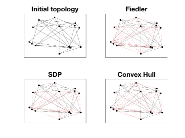
Figure 1: Initial topology of $14$ nodes and $28$ edges. Three methods are implemented to grow the network to $53$ edges, with the additional edges plotted as red dotted lines.

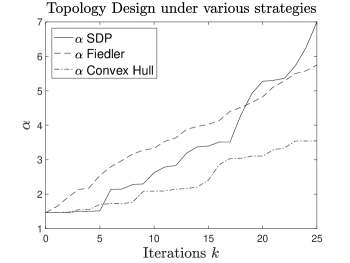
Figure 2: Performance each method over $k=25$ iterations.

Next, we study a small network of $7$ nodes and $11$ edges so that the solutions to $\operatorname{\mathsf{P}}2$ and $\operatorname{\mathsf{P}}3$ may be brute-forcibly computed to test Algorithms 1–3, with $\eta_{1}(k)$ being used for Algorithm 2. We choose $\mathop{\mathcal{P}}\nolimits=[0.25,0.75]^{11}\cap\{p\;|\;\sum_{l}p_{l}\leq 4.25\}$ and $\mathop{\mathcal{S}}\nolimits=\{0,1\}^{11}\cap\{s\;|\;\sum_{l}s_{l}\leq 5\}$. We run the algorithms for $T=30$ iterations and plot the results at each iteration in Figure 3.

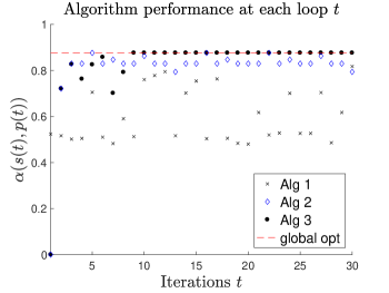
Figure 3: Performance of Algorithms 1–3 at each loop $t$.

Clearly, Algorithm 1 does not improve across iterations as it does not utilize information about the attacker’s plays from previous iterations, and it achieves a maximum value of $\alpha(s(t^{\star}),p(t^{\star}))=0.8175$, which is a bit below the global optimum $\alpha(s^{\star},p^{\star})=0.8762$. Algorithm 2 achieves the global optimum $\alpha(s(t^{\star}),p(t^{\star}))=0.8762$ the fastest, at $t^{\star}=5$, although it never reaches this point again and instead oscillates around suboptimal points, indicating that optimality may not be reliably attained in general. Counter-intuitively, the performance of Algorithm 3 does not improve monotonically in $t$, although this should be expected: early solutions $s(t)$ may get “lucky”, in some sense, but the subsequent iteration may allow the attacker to jump to a new vulnerable part of the space. Once the algorithm achieves the global optimum at $t^{\star}=9$, it does not dip below this for the remainder of the time horizon. Finally, we note that the behavior of each algorithm observed here is typical when implemented on other small graphs.

VII Concluding Remarks

This paper introduced three related problems motivated by studying the algebraic connectivity of a graph by adding edges to an initial topology or protecting edges under the case of a disturbance or attack on the network. We developed a novel SDP relaxation to address the NP-hardness of the design and demonstrated in simulation that it is superior to existing methods which are greedy and cannot accommodate general constraints. In addition, we studied the dynamics of the game that may be played between a network coordinator and strategic attacker. We developed the notion of an optimal preventive solution for the coordinator and proposed effective heuristics to find such a solution guided by characterizations of the solutions to the attacker’s problem. Future work includes characterizing the performance of our SDP relaxation and developing an algorithm which provably converges to the optimal preventive strategy.

References

- [1] S. Bhattacharya, A. Gupta, and T. Basar. Jamming in mobile networks: a game-theoretic approach. Numerical Algebra, Optimization, and Control, 3(1):1–30, 2013.
- [2] S. Boyd. Convex optimization of graph Laplacian eigenvalues. In Proc. Int. Congress of Mathematicians, volume 3, pages 1311–1319, 2006.
- [3] S. Boyd and L. Vandenberghe. Convex Optimization. Cambridge University Press, 2004.
- [4] CAISO Business Practice Manual for Market Operation, 2017. Version 51. Available at https://bpmcm.caiso.com/Pages/BPMDetails.aspx?BPM=Market%20Operations.
- [5] N. M. M. de Abreu. Old and new results on algebraic connectivity of graphs. Linear Algebra and Its Applications, 423(1):53–73, 2006.
- [6] X. Ding and T. Jiang. Spectral distributions of adjacency and Laplacian matrices of random graphs. The Annals of Applied Probability, 20(6):2086–2117, 2010.
- [7] M. Fiedler. Algebraic connectivity of graphs. Czechoslovak Mathematical Journal, 23(98):298–305, 1973.
- [8] A. Ghosh and S. Boyd. Growing well-connected graphs. In IEEE Int. Conf. on Decision and Control, pages 6605–6611, San Diego, USA, 2006.
- [9] C. D. Godsil and G. F. Royle. Algebraic Graph Theory, volume 207 of Graduate Texts in Mathematics. Springer, New York, 2001.
- [10] M. Goemans and D. Williamson. Improved approximation algorithms for maximum cut and satisfiability problems using semidefinite programming. Journal of the Association for Computing Machinery, 42(6):1115–1145, 1995.
- [11] R. Merris. Laplacian graph eigenvectors. Linear Algebra and Its Applications, 278:221–236, 1998.
- [12] J. Urschel, X. Hu, J. Xu, and L. Zikatanov. A cascadic multigrid algorithm for computing the Fiedler vector of graph Laplacians. Journal of Computational Mathematics, 33(2):209–226, 2015.
- [13] P. Yang, R. A. Freeman, G. J. Gordon, K. M. Lynch, S. S. Srinivasa, and R. Sukthankar. Decentralized estimation and control of graph connectivity for mobile sensor networks. Automatica, 46(2):390–396, 2010.