Enhancing Network Embedding with Auxiliary Information: An Explicit Matrix
Factorization Perspective

Abstract

Recent advances in the field of network embedding have shown the low-dimensional network representation is playing a critical role in network analysis. However, most of the existing principles of network embedding do not incorporate auxiliary information such as content and labels of nodes flexibly. In this paper, we take a matrix factorization perspective of network embedding, and incorporate structure, content and label information of the network simultaneously. For structure, we validate that the matrix we construct preserves high-order proximities of the network. Label information can be further integrated into the matrix via the process of random walk sampling to enhance the quality of embedding in an unsupervised manner, i.e., without leveraging downstream classifiers. In addition, we generalize the Skip-Gram Negative Sampling model to integrate the content of the network in a matrix factorization framework. As a consequence, network embedding can be learned in a unified framework integrating network structure and node content as well as label information simultaneously. We demonstrate the efficacy of the proposed model with the tasks of semi-supervised node classification and link prediction on a variety of real-world benchmark network datasets.

1 Introduction

The rapid growth of applications based on networks has posed major challenges of effective processing of network data, among which a critical task is network data representation. The primitive representation of a network is usually very sparse and suffers from overwhelming high dimensionality, which limits its generalization in statistical learning. To deal with this issue, network embedding aims to learn latent representations of nodes on a network while preserving the structure and the inherent properties of the network, which can be effectively exploited by classical vector-based machine learning models for tasks including node classification, link prediction, and community detection, etc. [6, 3, 10, 1].

Recently, inspired by the advances of neural representation learning in language modeling, which is based on the principle of learning the embedding vector of a word by predicting its context [12, 13], a number of network embedding approaches have been proposed with the paradigm of learning the embedding vector of a node by predicting its neighborhood [17, 20, 3]. Specifically, latent representations of network nodes are learned by treating short random walk sequences as sentences to encode structural proximity in a network. Existing results demonstrate the effectiveness of the neural network embedding approaches in the tasks of node classification, behavior prediction, etc.

However, existing network embedding methods, including DeepWalk [17], LINE [20] and node2vec [3], are typically based on structural proximities only and do not incorporate other information such as node content flexibly. In this paper, we explore the question whether network structure and auxiliary properties of the network such as node content and label information can be integrated in a unified framework of network embedding. To achieve that, we take a matrix factorization perspective of network embedding with the benefits of natural integration of structural embedding and content embedding simultaneously, where label information can be incorporated flexibly.

Specifically, motivated by the recent work [9] that explains the word embedding model of Skip-Gram Negative Sampling (SGNS) as a matrix factorization of the words’ co-occurrence matrix, we build a co-occurrence matrix of structural proximities for a network based on a random walk sampling procedure. The process of SGNS can then be formulated as minimizing a matrix factorization loss, which can be naturally integrated with representation learning of node content. In addition, label information can be exploited in the process of building the co-occurrence matrix to enhance the quality of network embedding, which is achieved by decomposing the context of a node into the structure context generated with random walks, as well as the label context based on the given label information.

Our main contributions can be summarized as follows:

• We propose a unified framework of Auxiliary information Preserved Network Embedding with matrix factorization, abbreviated as APNE, which can effectively learn the latent representations of nodes, and provide a flexible integration of network structure, node content, as well as label information without leveraging downstream classifiers.

• We verify that the structure matrix we generate is an approximation of the high-order proximity of the network known as rooted PageRank.

• We extensively evaluate our framework on four benchmark datasets and two tasks including semi-supervised classification and link prediction. Results show that the representations learned by our proposed method are general and powerful, producing significantly increased performance over the state of the art on both tasks.

2 Related Work

2.1 Network Embedding

Network embedding has been extensively studied in the literature [1]. Recently, motivated by the advances of neural representation learning in language modeling, a number of embedding learning methods have been proposed based on the Skip-Gram model. A representative model is DeepWalk [17], which exploits random walk to generate sequences of instances as the training corpus, followed by utilizing the Skip-Gram model to obtain the embedding vectors of nodes. Node2vec [3] extend DeepWalk with sophisticated random walk schemes. Similarly in LINE [20] and GraRep [2], network embedding is learned by directly optimizing the objective function inspired from the Skip-Gram model. To further incorporate auxiliary information into network embedding, many efforts have been made. Among them, TADW [22] formulates DeepWalk in a matrix factorization framework, and jointly learns embeddings with the structure information and preprocessed features of text information. This work is further extended by HSCA [25], DMF [24] and MMDW [21] with various additional information. In SPINE [4], structural identities are incorporated to jointly preserve local proximity and global proximity of the network simultaneously in the learned embeddings. However, none of the above models jointly consider structure, content and label information in a unified model, which are the fundamental elements of a network [1]. Recently, TriDNR [16] and LANE [5] tackle this problem both through implicit interactions between the three elements. TriDNR leverages multiple skip-gram algorithms between node-word and word-label pairs, while LANE first constructs three network affinity matrices from the three elements respectively, followed by executing SVD on affinity matrices with additional pairwise interactions. Although empirically effective, these methods do not provide a clear objective articulating how the three aspects are integrated in the embeddings learned, and is relatively inflexible to generalize to other scenarios.

In contrast to the above models, we propose a unified framework to learn network embeddings from structure, content and label simultaneously. The superiority of our framework is threefold: a) the structure matrix we generate contains high-order proximities of the network, and the label information is incorporated by explicitly manipulating the constructed matrix rather than through implicit multi-hop interactions [16, 5]; b) instead of leveraging label information through an explicitly learned classifier (e.g., SVM [21], linear classifier [24] and neural networks [23, 6]) whose performance is not only related to the quality of embeddings but also the specific classifiers being used, we exploit the label information without leveraging any downstream classifiers, which enables the flexibility of our model to generalize to different tasks; c) while most of the above models only consider text descriptions of nodes, we use raw features contained in datasets as the content information, which is more generalized to various types of networks in real world such as social networks.

2.2 Matrix Factorization and Word Embedding

Matrix Factorization (MF) has been proven effective in various machine learning tasks, such as dimensionality reduction, representation learning, recommendation systems, etc. Recently, connections have been built between MF and word embedding models. It is shown in [8] that the Skip-Gram with Negative Sampling (SGNS) model is an Implicit Matrix Factorization (IMF) that factorizes a word-context matrix, where the value of each entry is the pointwise mutual information (PMI) between a word and context pair, indicating the strength of association. It is further pointed out in [9] that the SGNS objective can be reformulated in a representation learning view with an Explicit Matrix Factorization (EMF) objective, where the matrix being factorized here is the co-occurrence matrix among words and contexts.

In this paper, we extend the matrix factorization perspective of word embedding into the task of network embedding. More importantly, we learn the network embedding by jointly factorizing the structure matrix and the content matrix of the network, which can be further improved by leveraging auxiliary label information. Different from most existing network embedding methods based on matrix factorization, which employ either trivial objective functions (F-norm used in TADW) or traditional factorization algorithms (SVD used in GraRep) for optimization, we design a novel objective function based on SGNS in our framework. Furthermore, the proposed method is general and not confined to specific downstream tasks, such as link prediction [3] and node classification [17], and we do not leverage any classifiers either.

3 Network Embedding with Matrix Factorization

Figure 1: The overall procedure of our framework (APNE). Different colors indicate different labels of nodes.

In this section, we propose a novel approach for network embedding based on a unified matrix factorization framework, which consists of three procedures as illustrated in Figure 1. We follow the paradigm of treating random walk sequences as sentences to encode structural proximities in a network. However, unlike the EMF objective for word embedding where the matrix to factorize is clearly defined as the word-context co-occurrence matrix, for network embedding, there is a gap between the random walk procedure and the co-occurrence matrix. Therefore, we start with proposing a random walk sampling process to build a co-occurrence matrix, followed by theoretical justification of its property of preserving the high-order structural proximity in the network, based on which we present the framework of network embedding with matrix factorization.

3.1 High-Order Proximity Preserving Matrix

Given an undirected network $G=\{V,E\}$ which includes a set of nodes $V$ connected by a set of edges $E$, the corresponding adjacency matrix is $\bm{A}$, where $A_{i,j}=w_{i,j}$ indicates an edge with weight $w_{i,j}$ between the $i$-th node $v_{i}$ and the $j$-th node $v_{j}$. And we denote the transition matrix of $G$ as $\bm{P}$, where $P_{i,j}=\frac{w_{i,j}}{\sum_{k=1}^{|V|}w_{i,k}}$. Next, a list of node sequences $C$ can be generated with random walks on the network.

Given $C$, we can generate the co-occurrence matrix $\bm{D}$ of $G$ with the $n$-gram algorithm. The procedure is summarized in Algorithm 1. In short, for a given node in a node sequence, we increase the co-occurrence count of two nodes if and only if they are in a window of size $l$.

Algorithm 1 Sampling the general co-occurrence matrix

0:  The transition matrix $\bm{P}$, window size $l$

0:  Co-occurrence matrix $\bm{D}$

1:  Sample random walks $C$ based on $\bm{P}$

2:  for every node sequence in $C$ do

3:     Uniformly sample $(i,j)$ with $|i-j|<l$

4:     $D_{v_{i},v_{j}}=D_{v_{i},v_{j}}+1$

5:  end for

Next we show that the co-occurrence matrix generated by Algorithm 1 preserves the high-order structural proximity in the network with the following theorem:

Theorem 3.1.

Define the high-order proximity $\bm{S}$ of the network $G$ as

$\bm{S^{l}}=\sum_{k=1}^{l}\bm{P}^{k}$

where $l$ denotes the order of the proximity as well as the window size in Algorithm 1. Then, under the condition that the random walk procedure is repeated enough times and the generated list of node sequences $C$ covers all paths in the network $G$, we can derive that according to [22]:

$$\small l\cdot\bm{D}^{nor}=\bm{S^{l}}$$ (1)

where $l$ is the window size in Algorithm 1, and the matrix $\bm{D}^{nor}$ denotes the expectation of row normalized co-occurrence matrix $\bm{D}$, i.e., $\bm{D}^{nor}_{i,j}=\mathbb{E}[\frac{\bm{D}_{i,j}}{\sum_{k=1}^{|V|}D_{i,k}}]$.

Note that the $(i,j)$-th entry of the left side of Equation (1) can be written as $\mathbb{E}[\frac{\bm{D}_{i,j}}{\sum_{k=1}^{|V|}D_{i,k}/l}]$, which is the expected number of times that $v_{j}$ appears in the left or right $l$-neighborhood of $v_{i}$.

To investigate into the structural information of the network encoded in the co-occurrence matrix $\bm{D}$, we first consider a well-known high-order proximity of a network named rooted PageRank (RPR) [19], defined as $\bm{S}^{\textrm{RPR}}=(1-\beta_{\textrm{RPR}})(\bm{I}-\beta_{\textrm{RPR}}\bm{P})^{-1}$, where $\beta_{\textrm{RPR}}\in(0,1)$ is the probability of randomly walking to a neighbor rather than jumping back. The $(i,j)$-th entry of $\bm{S}^{\textrm{RPR}}$ is the probability that a random walk from node $v_{i}$ will stop at $v_{j}$ in the steady state, which can be used as an indicator of the node-to-node proximity. $\bm{S}^{\textrm{RPR}}$ can be further rewritten as:

$$\bm{S}^{\textrm{RPR}}= (1-\beta_{\textrm{RPR}})(\bm{I}-\beta_{\textrm{RPR}}\bm{P})^{-1}$$ (2)

$$= (1-\beta_{\textrm{RPR}})\sum_{k=0}^{\infty}\beta_{\textrm{RPR}}^{k}\bm{P}^{k}$$ (3)

We next show that for an undirected network, where $\bm{P}$ is symmetric, the row normalized co-occurrence matrix $\bm{D}^{nor}$ is an approximation of the rooted PageRank matrix $\bm{S}^{\textrm{RPR}}$.

Theorem 3.2.

When $l$ is sufficiently large, for $\bm{D}^{nor}$ defined as $\bm{D}^{nor}=\frac{1}{l}\sum_{k=1}^{l}\bm{P}^{k}$, and $K=\lfloor-\frac{\log l(1-\beta_{\textrm{RPR}})}{\log\beta_{\textrm{RPR}}}\rfloor$, the $\ell$-2 norm of the difference between $\bm{D}^{nor}$ and $\bm{S}^{\textrm{RPR}}$ can be bounded by $K$:

$$\small\left\lVert\bm{S}^{\textrm{RPR}}-\bm{D}^{nor}\right\rVert_{2}\leq 2-2\beta_{\textrm{RPR}}^{K+1}$$ (4)

Proof of Theorem 3.2.    Here we omit the superscript of $\bm{S}^{\textrm{RPR}}$ and the subscript of $\beta_{\textrm{RPR}}$ in the proof for simplicity. Substituting (2) and reformulating the left side of (4) we have:

$$\left\lVert\bm{S}-\bm{D}^{nor}\right\rVert_{2}=\left\lVert(1-\beta)\sum_{k=0}^{\infty}\beta^{k}\bm{P}^{k}-\frac{1}{l}\sum_{k=1}^{l}\bm{P}^{k}\right\rVert_{2}$$

$$=\left\lVert(1-\beta)\sum_{k=0}^{l}\beta^{k}\bm{P}^{k}-\frac{1}{l}\sum_{k=0}^{l}\bm{P}^{k}+\frac{1}{l}+(1-\beta)\sum_{k=l+1}^{\infty}\beta^{k}\bm{P}^{k}\right\rVert_{2}$$

$$\leq\left\lVert\sum_{k=0}^{l}\bm{P}^{k}\left[(1-\beta)\beta^{k}-\frac{1}{l}\right]\right\rVert_{2}+(1-\beta)\left\lVert\sum_{k=l+1}^{\infty}\beta^{k}\bm{P}^{k}\right\rVert_{2}+\frac{1}{l}$$

$$\leq\sum_{k=0}^{l}\lambda_{\max}^{k}\left|(1-\beta)\beta^{k}-\frac{1}{l}\right|+(1-\beta)\sum_{k=l+1}^{\infty}\beta^{k}\lambda_{\max}^{k}+\frac{1}{l}$$

where $\lambda_{\max}$ is the largest singular value of matrix $\bm{P}$, which is also the eigenvalue of $\bm{P}$ for the reason that $\bm{P}$ is symmetric and non-negative. Note that $\bm{P}$ is the transition matrix, which is also known as the Markov matrix. And it can be easily proven that the largest eigenvalue of a Markov matrix is always $1$, i.e., $\lambda_{\max}=1$. We eliminate the absolute value sign by splitting the summation at $K=\lfloor-\frac{\log l(1-\beta)}{\log\beta}\rfloor$, then we have:

$$\left\lVert\bm{S}-\bm{D}^{nor}\right\rVert_{2} \leq\sum_{k=0}^{K}\left[(1-\beta)\beta^{k}-\frac{1}{l}\right]+\sum_{k=K+1}^{l}\left[\frac{1}{l}-(1-\beta)\beta^{k}\right]$$

$$+(1-\beta)\sum_{k=l+1}^{\infty}\beta^{k}+\frac{1}{l}$$

$$=1-\beta^{K+1}-\beta^{K+1}(1-\beta^{l-K})+\frac{l-2K}{l}+\beta^{l+1}$$

$$=1-2\beta^{K+1}+2\beta^{l+1}+\frac{l-2K}{l}$$

Note that when $l$ is sufficiently large, according to the definition of $K$, we have $K\ll l$. Given $\beta\in(0,1)$, we can derive:

$$\small\left\lVert\bm{S}-\bm{D}^{nor}\right\rVert_{2}\leq 2-2\beta^{K+1}.$$

$\hfill\qed$

With Theorem 3.2, we can conclude that the normalized co-occurrence matrix $\bm{D}^{nor}$ we construct is an approximation of the rooted PageRank matrix $S^{\textrm{RPR}}$ with a bounded $\ell$-2 norm.

Note that in TADW [22] and its follow-up works [25, 24] which also apply matrix factorization to learn network embeddings, the matrix constructed to represent the structure of a network is $\frac{\bm{P}+\bm{P}^{2}}{2}$, which is a special case of $\bm{D}^{nor}$ when $l=2$. As comparison, we construct a general matrix while preserving high-order proximities of the network with theoretical justification.

3.2 Incorporating Label Context

Algorithm 2 Sampling general co-occurrence matrix with structure and label context

0:  The transition matrix $\bm{P}$, labeled nodes $L$, parameters $m$, $l$, $d$

0:  Co-occurrence matrix $\bm{D}$

1:  Sample random walks ${C}$ of length $d$ based on $\bm{P}$

2:  for every node sequence in $C$ do

3:     Uniformly sample $(i,j)$ with $|i-j|<l$

4:     $D_{v_{i},v_{j}}=D_{v_{i},v_{j}}+1$

5:  end for

6:  for $k=1$ to $m$ do

7:     Uniformly sample a node $v_{i}$ in $L$

8:     Uniformly sample a node $v_{j}$ with the same label as node $v_{i}$

9:     $D_{v_{i},v_{j}}=D_{v_{i},v_{j}}+1$

10:  end for

Apparently, the co-occurrence value between node $v_{i}$ and context $v_{c}$ indicates the similarity between them. A larger value of co-occurrence indicates closer proximity in the network, hence higher probability of belonging to the same class. This intuition coincides with the label information of nodes. Therefore, with the benefit of integer values in $\bm{D}$, label information can be explicitly incorporated in the procedure of sampling $\bm{D}$ to enhance the proximity between nodes, which can additionally alleviate the problem of isolated nodes without co-occurrence in structure, i.e., we consider isolated nodes through label context instead of structure context.

Specifically, we randomly sample one node among labeled instances, followed by uniformly choosing another node with the same label and update the corresponding co-occurrence count in $\bm{D}$. As a consequence, the co-occurrence matrix $\bm{D}$ captures both structure co-occurrence and label co-occurrence of instances. The complete procedure is summarized in Algorithm 2, where $m$ is a parameter controlling the ratio between the structure and label context.

In this way, while preserving high-order proximities of the network, we can incorporate supervision into the model flexibly without leveraging any downstream classifiers, which is another important advantage of our method. By contrast, most existing methods are either purely unsupervised [22] or leveraging label information through downstream classifiers [21, 24].

3.3 Joint Matrix Factorization

The method proposed above generates the co-occurrence matrix from a network and bridges the gap between word embedding and network embedding, allowing us to apply the matrix factorization paradigm to network embedding. With the flexibility of the matrix factorization principle, we propose a joint matrix factorization model that can learn network embeddings exploiting not only the topological structure and label information but also the content information of the network simultaneously.

Given the co-occurrence matrix $\bm{D}\in\mathbb{R}^{|V|\times|V|}$ and the content matrix $\bm{F}\in\mathbb{R}^{N_{f}\times|V|}$, where $|V|$ and $N_{f}$ represent the number of nodes in the network and the dimensionality of node features respectively. Let $d$ be the dimensionality of embedding. The objective here is to learn the embedding of a network $G$, denoted as the matrix $\bm{W}\in\mathbb{R}^{d\times|V|}$, by minimizing the loss of factorizing the matrices $\bm{D}$ and $\bm{F}$ jointly as:

$$\small\min_{\bm{W},\bm{S}}MF(\bm{D},\bm{F}^{T}\bm{S}\bm{W})$$ (5)

where $MF(\cdot,\cdot)$ is the reconstruction loss of matrix factorization which will be introduced later, and $\bm{S}\in\mathbb{R}^{N_{f}\times d}$ can be regarded as the feature embedding matrix, thus $\bm{F}^{T}\bm{S}$ is the feature embedding dictionary of nodes.

By solving the joint matrix factorization problem in (5), the structure information in $\bm{D}$ and the content information in $\bm{F}$ are integrated to learn the network embeddings $\bm{W}$. This is inspired by Inductive Matrix Completion [14], a method originally proposed to complete a gene-disease matrix with gene and disease features. However, we take a completely different loss function here in light of the word embedding model of SGNS with a matrix factorization perspective [9].

We first rewrite (5) in a representation learning view as:

$$\small\min_{\bm{W},\bm{S}}\sum_{i}MF(\bm{d_{i}},\bm{F}^{T}\bm{S}\bm{w_{i}})$$ (6)

where $MF(\cdot,\cdot)$ is the representation loss functions evaluating the discrepancy between the $i^{th}$ column of $\bm{D}$ and $\bm{F}^{T}\bm{S}\bm{W}$. $\bm{F}^{T}\bm{S}$ is the feature embedding dictionary, and the embedding vector of the $i^{th}$ node, $\bm{w_{i}}\in\mathbb{R}^{d}$, can be learned by minimizing the loss of representing its structure context vector $\bm{d_{i}}$ via the feature embedding $\bm{F}^{T}\bm{S}$.

We then proceed to the objective of factorizing the co-occurrence matrix $\bm{D}$ and the content matrix $\bm{F}$ jointly, denoted as $MF(\bm{d_{i}},\bm{F}^{T}\bm{S}\bm{w_{i}})$. We follow the paradigm of explicit matrix factorization of the SGNS model and derive the following theorem according to [9]:

Theorem 3.3.

For a node $i$ in the network, we denote $Q_{i,c}$ as a pre-defined upper bound for the possible co-occurrence count between node $i$ and context $c$. With the equivalence of Skip-Gram Negative Sampling (SGNS) and Explicit Matrix Factorization (EMF) [9], the representation loss $MF(\cdot,\cdot)$ can be defined as the negative log probability of observing the structure vector $\bm{d_{i}}$ given $i$ and $\bm{F}^{T}\bm{S}$ when $Q_{i,c}$ is set to $k\frac{\#(i)\#(c)}{|D|}+\#(i,c)$. To be more concrete,

$MF(\bm{d_{i}},\bm{F}^{T}\bm{S}\bm{w_{i}})=-\sum_{c\in|V|}\log P(d_{i,c}|\bm{f}^{T}_{c}\bm{S}\bm{w_{i}})$

where $\bm{f}_{c}\in\mathbb{R}^{N_{f}}$ is the $c$-th column of the content matrix $\bm{F}$, i.e., the feature vector of node $c$, $\#(i,c)$ is the co-occurrence count between node $i$ and $c$, $\#(i)=\sum_{c\in|V|}\#(i,c)$, $\#(c)=\sum_{i\in|V|}\#(i,c)$, $|D|=\sum_{i,c\in|V|}\#(i,c)$ and $k$ is the negative sampling ratio.

Based on Theorem 3.3, we can derive:

$$MF(\bm{D},\bm{F}^{T}\bm{S}\bm{W}) \triangleq\sum_{i=1}^{|V|}MF(\bm{d_{i}},\bm{F}^{T}\bm{S}\bm{w_{i}})$$

$$=-\sum_{i=1}^{|V|}\sum_{c=1}^{|V|}\log P(d_{i,c}|\bm{f}^{T}_{c}\bm{S}\bm{w_{i}})$$

Finally, we can formulate the objective of the joint matrix factorization framework with parameters $\bm{W}$ and $\bm{S}$ as:

$$L(\bm{W},\bm{S}) =MF(\bm{D},\bm{F}^{T}\bm{S}\bm{W})$$ (7)

$$=-\sum_{i=1}^{|V|}\sum_{c=1}^{|V|}\log P(d_{i,c}|\bm{f}^{T}_{c}\bm{S}\bm{w_{i}})$$

3.4 Optimization

To minimize the loss function in (7) which integrates structure, label and content simultaneously, we utilize a novel optimization algorithm leveraging the alternating minimization scheme (ALM), which is a widely adopted method in the matrix factorization literature.

First we derive the gradients of (7) as:

$$\frac{\partial L(\bm{W},\bm{S})}{\partial\bm{S}} =\frac{\partial MF(\bm{D},\bm{F}^{T}\bm{S}\bm{W})}{\partial\bm{S}}$$

$$=\sum_{i\in|V|}-\bm{d_{i}}\bm{w_{i}}^{T}+\mathbb{E}_{\bm{d_{i}}^{{}^{\prime}}|\bm{F}^{T}\bm{S}\bm{w_{i}}}[\bm{d_{i}}^{{}^{\prime}}]\bm{w_{i}}^{T}$$

$$=\bm{F}(\mathbb{E}_{\bm{D}^{{}^{\prime}}|\bm{F}^{T}\bm{S}\bm{W}}\bm{D}^{{}^{\prime}}-\bm{D})\bm{W}^{T}$$

$$\triangleq\mathrm{grad}_{\bm{S}}$$

$$\frac{\partial L(\bm{W},\bm{S})}{\partial\bm{W}} =\bm{S}^{T}\bm{F}(\mathbb{E}_{\bm{D}^{{}^{\prime}}|\bm{F}^{T}\bm{S}\bm{W}}\bm{D}^{{}^{\prime}}-\bm{D})$$

$$\triangleq\mathrm{grad}_{\bm{W}}$$

We denote $\mathrm{grad}_{\bm{W}}$ and $\mathrm{grad}_{\bm{S}}$ as the gradients of $\bm{W}$ and $\bm{S}$ in the loss function (7) respectively. Note that the expectation $\mathbb{E}_{\bm{d_{i}}^{{}^{\prime}}|\bm{F}^{T}\bm{S}\bm{w_{i}}}$ can be computed in a closed form [9] as:

$$\small\mathbb{E}_{d_{i,c}^{{}^{\prime}}|\bm{f}^{T}_{c}\bm{S}\bm{w_{i}}}[d_{i,c}^{{}^{\prime}}]=Q_{i,c}\sigma(\bm{f}^{T}_{c}\bm{S}\bm{w_{i}})$$ (8)

where $\sigma(x)=\frac{1}{1+e^{-x}}$ is the sigmoid function.

The algorithm of Alternating Minimization (ALM) is summarized in Algorithm 3. The algorithm can be divided into solving two convex subproblems (starting from line 3 and line 6 respectively), which guarantees that the optimal solution of each subproblem can be reached with sublinear convergence rate with a properly chosen step-size [15]. One can easily show that the objective (7) descents monotonically. As a consequence, Algorithm 3 will converge due to the lower bounded objective function (7).

The time complexity of one iteration in Algorithm 3 is $O((nnz(\bm{F})d|V|)^{2})$, where $nnz(\bm{F})$ is the number of non-zero elements in $\bm{F}$. For datasets with sparse node content, e.g., Cora, Citeseer, Facebook, etc., we implement $\bm{f}^{T}_{c}\bm{S}$ in Equation (8) efficiently as a product of a sparse matrix with a dense matrix, which reduces the complexity from $O(|V|N_{f}d)$ to $O(nnz(\bm{F})d)$.

Algorithm 3 ALM algorithm for generalized explicit matrix factorization

0:  Co-occurrence matrix $\bm{D}$, content matrix $\bm{F}$, ALM step-size $\mu$ and maximum number of outer iterations $I$

0:  Node embedding matrix $\bm{W}$, feature embedding dictionary $\bm{S}$

1:  Initialize $\bm{W}$ and $\bm{S}$ randomly

2:  for $i=1$ to $I$ do

3:     repeat

4:        $\bm{W}=\bm{W}-\mu\cdot\mathrm{grad}_{\bm{W}}$

5:     until Convergence

6:     repeat

7:        $\bm{S}=\bm{S}-\mu\cdot\mathrm{grad}_{\bm{S}}$

8:     until Convergence

9:  end for

4 Experiments

The proposed framework is independent of specific downstream tasks, therefore in experiments, we test the model with different tasks including link prediction and node classification. Below we first introduce the datasets we use and the baseline methods that we compare to.

Table 1: Dataset statistics

Dataset	# Classes	# Nodes	# Edges	# Feature
Citeseer	$6$	$3327$	$4732$	$3703$
Cora	$7$	$2708$	$5429$	$1433$
Pubmed	$3$	$19717$	$44338$	$500$
Facebook	-	$4309$	$88234$	$1283$

Datasets.  We test our models on four benchmark datasets. The statistics of datasets are summarized in Table 1. For the node classification task, we employ datasets of Citation Networks [18], where nodes represent papers while edges represent citations. And each paper is described by a one-hot vector or a TFIDF word vector. For the link prediction task, we additionally include a social network dataset Facebook [7]. This dataset consists of $10$ ego-networks from the online social network Facebook, where nodes and edges represent users and their relations respectively. Each user is described by users’ properties, which is represented by a one-hot vector.

Baselines.  For both tasks, we compare our method with network embedding algorithms including DeepWalk [17], node2vec [3], TADW [22] and HSCA [25]. For the node classification task, we further include DMF [24], LANE [5] and two neural network based methods, Planetoid [23] and GCN [6]. To measure the performance of link prediction, we also evaluate our method against some popular heuristic scores defined in node2vec [3]. Note that we do not consider TriDNR [16] as a baseline for the reason that they use text description as node content in citation networks, while in social networks such as Facebook, there is no natural text description for each user, which prevents TriDNR from generalizing to various types of networks. In addition, as MMDW [21] and DMF [24] are both semi-supervised variants of TADW with similar performance in our setting, we only compare our model with DMF for brevity.

Experimental Setup.  For our model, the hyper-parameters are tuned on the Citeseer dataset and kept on the others. The dimensionality of embedding is set to $200$ for the proposed methods. In terms of the optimization parameters, the number of iterations is set to $200$, the step-size in Algorithm 3 is set to $1e-7$. The parameters in Algorithm 2 are set in consistency with DeepWalk, i.e., walk length $d=40$ with window size $l=5$. We use APNE to denote our unsupervised model of network embedding where the co-occurrence matrix is generated by Algorithm 1, and APNE+label denotes the semi-supervised model which uses Algorithm 2 to incorporate label context into the co-occurrence matrix. Unless otherwise specified, in all the experiments, we use one-vs-rest logistic regression as the classifier for the embedding based methods.

4.1 Semi-supervised Node Classification

Table 2: Accuracy of semi-supervised node classification (in percentage). Upper and lower rows correspond to unsupervised and semi-supervised embedding methods respectively.

Method	Citeseer	Cora	Pubmed
DeepWalk	$41.5$	$67.3$	$66.4$
node2vec	$47.2$	$69.8$	$70.3$
TADW	$54.0$	$72.0$	$41.7$
HSCA	$47.7$	$65.4$	$41.7$
APNE	$\bm{72.6}$	$\bm{79.3}$	$\bm{81.5}$
DMF	$65.5$	$58.5$	$59.3$
LANE	$60.3$	$65.2$	-
Planetoid	$67.3$	$73.4$	$76.7$
GCN	$70.3$	$\bm{81.5}$	$79.0$
APNE+label	$\bm{72.8}$	$79.6$	$\bm{82.1}$

We first consider the semi-supervised node classification task on three citation network datasets. To facilitate the comparison between our model and the baselines, we use the same partition scheme of training set and test set as in [23]. To be concrete, we randomly sample $20$ instances from each class as training data, and $1000$ instances from all samples in the rest of the dataset as test data.

The experimental results are reported in Table 2. In the comparison of unsupervised models, the proposed APNE method learns embeddings from the network structure and node content jointly in a unified matrix factorization framework. As a consequence, APNE outperforms notably on all datasets with improvement from $10.1\%$ to $34.4\%$. Compared with TADW and HSCA, which both incorporate network topology and text features of nodes in a matrix factorization model simultaneously, our method is superior in the following: a) the matrix we construct and factorize represents the network topology better as proven in Section 3.1; b) the loss function we derive from SGNS is tailored for representation learning.

Meanwhile, in the comparison of semi-supervised methods, the proposed APNE model outperforms embedding based baselines significantly, illustrating the promotion brought by explicitly manipulating the constructed matrix rather than implicitly executing multi-hop interactions. In addition, LANE suffers from extensive complexity both in time and space, which prevents it from being generalized to larger networks such as Pubmed. Although being slightly inferior to GCN on the Cora dataset, considering that APNE is a feature learning method independent of downstream tasks and classifiers, the competitive results against the state-of-the-art CNN based method GCN justify that the node representations learned by APNE preserve the network information well.

In general, the proposed matrix factorization framework outperforms embedding based baselines and performs competitive with the state-of-the-art CNN based model, demonstrating the quality of embeddings learned by our methods to represent the network from the aspects of content and structure. Between the two variants of our proposed framework, APNE and APNE+label, the latter performs consistently better on all datasets, indicating the benefits of incorporating label context.

(a) APNE

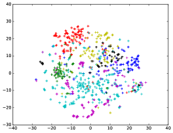
(b) node2vec

(c) TADW

Figure 2: t-SNE visualization of embeddings on Cora

We further visualize the embeddings learned by our unsupervised model APNE and two unsupervised embedding-based baselines on the Cora dataset with a widely-used dimension reduction method t-SNE [11], and results are shown in Figure 2. One can observe that different classes are better separated by our model, and nodes in the same class are clustered more tightly.

Figure 3: Parameter effect of APNE on the node classification task (in percentage)

In order to test the sensitivity of our framework to hyper-parameters, we choose different values of the negative sampling parameter $k$ in Theorem 3.3 and the number of iterations of label context sampling $m$ in Algorithm 2 and evaluate the model on Citeseer on the node classification task.

For each pair of parameters, we repeat the experiments 10 times and compute the mean accuracy. Results are shown in Figure 3. The horizontal axis represents different values of $m$. And $m=0$ represents results when the model is purely unsupervised, otherwise results are from semi-supervised models. The vertical axis is the classification accuracy on Citeseer. Clearly, increasing $m$ brings a boost of the performance of the model, as we infer in Section 3.2. This justifies the effectiveness of the approach we propose to incorporate the label context. In addition, the performance of the proposed models with different values of $k$ is relatively stable.

4.2 Link Prediction

Table 3: Results of link prediction

Method	Citeseer		Cora		Pubmed		Facebook
	AUC	MAP	AUC	MAP	AUC	MAP	AUC	MAP
Common Neighbor	$0.567$	$0.781$	$0.616$	$0.797$	$0.561$	$0.778$	$0.797$	$0.882$
Jaccard’s Coefficient	$0.567$	$0.782$	$0.616$	$0.795$	$0.561$	$0.776$	$0.797$	$0.877$
Adamic Adar	$0.560$	$0.780$	$0.617$	$0.801$	$0.561$	$0.778$	$0.798$	$0.885$
Preferential Attachment	$0.675$	$0.721$	$0.679$	$0.705$	$0.863$	$0.852$	$0.675$	$0.675$
DeepWalk	$0.656$	$0.725$	$0.734$	$0.793$	$0.721$	$0.781$	$0.891$	$0.914$
node2vec	$0.502$	$0.731$	$0.723$	$0.790$	$0.728$	$0.785$	$0.888$	$0.911$
TADW	$0.914$	$0.936$	$0.854$	$0.878$	$0.592$	$0.620$	$0.909$	$0.921$
HSCA	$0.905$	$0.928$	$0.861$	$0.885$	$0.632$	$0.660$	$0.926$	$0.917$
APNE	$\bm{0.938}$	$\bm{0.940}$	$\bm{0.909}$	$\bm{0.910}$	$\bm{0.925}$	$\bm{0.916}$	$\bm{0.956}$	$\bm{0.949}$

We further test our unsupervised model on the link prediction task. In link prediction, a snap-shot of the current network is given, and we are going to predict edges that will be added in the future. The experiment is set up as follows: we first remove $50\%$ of existing edges from the network randomly as positive node pairs, while ensuring the residual network connected. To generate negative examples, we randomly sample an equal number of node pairs that are not connected. Node representations are then learned based on the residual network. While testing, given a node pair in the samples, we compute the cosine similarity between their representation vectors as the edge’s score. Finally, Area Under Curve (AUC) score and Mean Average Precision (MAP) are used to evaluate the consistency between the labels and the similarity scores of the samples.

Results are summarized in Table 3. As shown in the table, our method APNE outperforms all the baselines consistently with different evaluation metrics. We take a lead of topology-only methods by a large margin, especially on sparser networks such as Citeseer, which indicates the importance of leveraging node features on networks with high sparsity. Again, we consistently outperform TADW and HSCA which also consider text features of nodes.

The stable performance of our proposed APNE model on different datasets justify that embeddings learned by jointly factorizing the co-occurrence matrix $\bm{D}$ and node features $\bm{F}$ can effectively represent the network. More importantly, the problem of sparsity can be alleviated by incorporating node features in a unified framework.

4.3 Case Study

Table 4: Two randomly chosen node pairs from Cora dataset

Title	Same Class	Connected	Cosine Similarity
			APNE	TADW
A cooperative coevolutionary approach to function	$\surd$	$\surd$	$\bm{0.471}$	$-0.002$
Multi-parent reproduction in genetic algorithms
A Class of Algorithms for Identification in $H_{\infty}$	$\surd$	$\times$	$\bm{0.158}$	$-0.129$
On the Computational Power of Neural Nets

To further illustrate the effectiveness of APNE, we present some instances of link prediction on the Cora dataset. We randomly choose $2$ node pairs from all node samples and compute the cosine similarity for each pair. Results are summarized in Table 4. The superiority of APNE is obvious in the first instance, where TADW gives a negative correlation to a positive pair. For this pair, although the first paper is cited by the second one, their neighbors do not coincide. As a consequence it is easy to wrongly separate these two nodes into different categories if the structure information is not sufficiently exploited.

As for the second instance, both papers belong to the Neural Networks class but not connected in the network. Specifically, the first paper focuses on H-Infinity methods in control theory while the second paper is about recurrent neural networks, and there exist papers linking these two domains together in the dataset. As a consequence, although these two nodes can hardly co-occur in random walk sequences on the network, their features may overlap in the dataset. Therefore, the pair of nodes will have a higher feature similarity than the topology similarity. Thus by jointly considering the network topology and the node features, our method gives a higher correlation score to the two nodes that are disconnected but belong to the same category.

5 Conclusion

In this paper, we aim to learn a generalized network embedding preserving structure, content and label information simultaneously. We propose a unified matrix factorization based framework which provides a flexible integration of network structure, node content, as well as label information. We bridge the gap between word embedding and network embedding by designing a method to generate the co-occurrence matrix from the network, which is actually an approximation of high-order proximities of nodes in the network. The experimental results on four benchmark datasets show that the joint matrix factorization method we propose brings substantial improvement over existing methods. One of our future directions would be to apply our framework to social recommendations to combine the relationship between users with the corresponding feature representations.

References

- [1] Cai, H., Zheng, V.W., Chang, K.C.C.: A comprehensive survey of graph embedding: Problems, techniques and applications. preprint arXiv:1709.07604 (2017)
- [2] Cao, S., Lu, W., Xu, Q.: Grarep: Learning graph representations with global structural information. In: Proceedings of the 24th ACM International on Conference on Information and Knowledge Management. pp. 891–900. ACM (2015)
- [3] Grover, A., Leskovec, J.: node2vec: Scalable feature learning for networks. In: Proceedings of the 22nd ACM SIGKDD International Conference on Knowledge Discovery and Data Mining. pp. 855–864. ACM (2016)
- [4] Guo, J., Xu, L., Chen, E.: Spine: Structural identity preserved inductive network embedding. arXiv preprint arXiv:1802.03984 (2018)
- [5] Huang, X., Li, J., Hu, X.: Label informed attributed network embedding. In: Proceedings of the Tenth ACM International Conference on Web Search and Data Mining. pp. 731–739. ACM (2017)
- [6] Kipf, T.N., Welling, M.: Semi-supervised classification with graph convolutional networks. arXiv preprint arXiv:1609.02907 (2016)
- [7] Leskovec, J., Krevl, A.: SNAP Datasets: Stanford large network dataset collection. http://snap.stanford.edu/data (Jun 2014)
- [8] Levy, O., Goldberg, Y.: Neural word embedding as implicit matrix factorization. In: Advances in neural information processing systems. pp. 2177–2185 (2014)
- [9] Li, Y., Xu, L., Tian, F., Jiang, L., Zhong, X., Chen, E.: Word embedding revisited: A new representation learning and explicit matrix factorization perspective. In: IJCAI 2015. pp. 3650–3656 (2015)
- [10] Liu, L., Xu, L., Wangy, Z., Chen, E.: Community detection based on structure and content: A content propagation perspective. In: IEEE International Conference on Data Mining (ICDM), 2015. pp. 271–280. IEEE (2015)
- [11] Maaten, L.v.d., Hinton, G.: Visualizing data using t-sne. Journal of Machine Learning Research 9(Nov), 2579–2605 (2008)
- [12] Mikolov, T., Chen, K., Corrado, G., Dean, J.: Efficient estimation of word representations in vector space. arXiv preprint arXiv:1301.3781 (2013)
- [13] Mikolov, T., Sutskever, I., Chen, K., Corrado, G.S., Dean, J.: Distributed representations of words and phrases and their compositionality. In: Advances in neural information processing systems. pp. 3111–3119 (2013)
- [14] Natarajan, N., Dhillon, I.S.: Inductive matrix completion for predicting gene–disease associations. Bioinformatics 30(12), i60–i68 (2014)
- [15] Nesterov, Y.: Introductory lectures on convex optimization: A basic course, vol. 87. Springer Science & Business Media (2013)
- [16] Pan, S., Wu, J., Zhu, X., Zhang, C., Wang, Y.: Tri-party deep network representation. Network 11(9), 12 (2016)
- [17] Perozzi, B., Al-Rfou, R., Skiena, S.: Deepwalk: Online learning of social representations. In: Proceedings of the 20th ACM SIGKDD International Conference on Knowledge Discovery and Data Mining. pp. 701–710. ACM (2014)
- [18] Sen, P., Namata, G., Bilgic, M., Getoor, L., Galligher, B., Eliassi-Rad, T.: Collective classification in network data. AI magazine 29(3), 93 (2008)
- [19] Song, H.H., Cho, T.W., Dave, V., Zhang, Y., Qiu, L.: Scalable proximity estimation and link prediction in online social networks. In: Proceedings of the 9th ACM SIGCOMM conference on Internet measurement conference. ACM (2009)
- [20] Tang, J., Qu, M., Wang, M., Zhang, M., Yan, J., Mei, Q.: Line: Large-scale information network embedding. In: Proceedings of the 24th International Conference on World Wide Web. pp. 1067–1077. ACM (2015)
- [21] Tu, C., Zhang, W., Liu, Z., Sun, M.: Max-margin deepwalk: discriminative learning of network representation. In: IJCAI 2016. pp. 3889–3895 (2016)
- [22] Yang, C., Liu, Z., Zhao, D., Sun, M., Chang, E.: Network representation learning with rich text information. In: IJCAI 2015 (2015)
- [23] Yang, Z., Cohen, W., Salakhutdinov, R.: Revisiting semi-supervised learning with graph embeddings. arXiv preprint arXiv:1603.08861 (2016)
- [24] Zhang, D., Yin, J., Zhu, X., Zhang, C.: Collective classification via discriminative matrix factorization on sparsely labeled networks. In: Proceedings of the 25th ACM International on Conference on Information and Knowledge Management. pp. 1563–1572. ACM (2016)
- [25] Zhang, D., Yin, J., Zhu, X., Zhang, C.: Homophily, structure, and content augmented network representation learning. In: IEEE 16th International Conference on Data Mining (ICDM), 2016. pp. 609–618. IEEE (2016)