Covariant Extension of the GPD overlap representation at low Fock states

Abstract

We present a novel approach to compute Generalized Parton Distributions within the Lightfront Wave Function overlap framework. We show how to systematically extend Generalized Parton Distributions computed within the DGLAP region to the ERBL one, fulfilling at the same time both the polynomiality and positivity conditions. We exemplify our method using pion Lightfront Wave Functions inspired by recent results of non-perturbative continuum techniques and algebraic nucleon Lightfront Wave Functions. We also test the robustness of our algorithm on reggeized phenomenological parameterizations. This approach paves the way to a better understanding of the nucleon structure from non-perturbative techniques and to a unification of Generalized Parton Distributions and Transverse Momentum Dependent Parton Distribution Functions phenomenology through Lightfront Wave Functions.

I Introduction

Generalized Parton Distributions (GPDs) were introduced two decades ago Mueller et al. (1994); Ji (1997); Radyushkin (1997) and have been since then a topic of strong interest in the hadron physics community, both on the theoretical and experimental side Ji (1998); Goeke et al. (2001); Diehl (2003); Belitsky and Radyushkin (2005); Boffi and Pasquini (2007); Guidal et al. (2013); Mueller (2014). A significant amount of beam time of the upgraded Jefferson Laboratory facility is dedicated to their experimental study and they are one of the core scientific cases for building the U.S. Electron-Ion Collider (EIC). Not only are they an elegant way to unify both Parton Distribution Functions (PDFs) and Form Factors into a single object, leading to a three-dimensional picture of hadrons Burkardt (2000), but they also provide genuine information and constraints through their skewness dependence. If these constraints have been used to produce phenomenological models Guidal et al. (2005); Goloskokov and Kroll (2005); Polyakov and Semenov-Tian-Shansky (2009); Kumerički and Mueller (2010); Goldstein et al. (2011), none of these models is built within a formalism guaranteeing a priori all the constraints to be fulfilled at the same time. The same problems also appears from non-perturbative computations of GPDs using various techniques (see e.g. Ref. Mezrag et al. (2016); Tiburzi and Verma (2017) and refs therein), and only in very few cases particular models have taken care of both constraints (see e.g. Refs. Broniowski et al. (2008); Dorokhov et al. (2011)).

In this paper, we focus on two of them, the so-called polynomiality and positivity properties. The former states that the Mellin Moments of the GPDs are polynomials (of definite degree) of the skewness. It comes from the Lorentz structure of the matrix elements of local operators defining these Mellin moments. On the other hand, positivity gives an upper bound on the absolute value of GPDs taken at a given kinematics in terms of PDFs. This property can be derived from Hilbert space norms. Consequently, covariant approaches usually successfully recover polynomiality but have hard time dealing with positivity. On the other hand, quantum mechanical based techniques, like Fock states expansions, have the positivity property “built-in” but usually fail at getting polynomial Mellin moments. Facing this issue, model builders have generally to favor one of these two fundamental properties, at the risk of violating the other.

We present here a general solution to this problem. Section II will remind the reader the details and subtleties of modeling GPDs through the ways mentioned above. Section III introduces the theory behind our technique, while in section IV we present our method, based on the numerical inversion of the Radon transform with incomplete data. Section V is then dedicated to the applications of our algorithm to different examples of Lightfront Wave Functions (LFWFs). In section VI we discuss our results and the phenomenological relevance of ambiguities related to the inverse of the Radon transform. Section VII concludes this paper.

II GPD Theory and Modeling

GPDs are defined as a Lightfront projection of a non-diagonal hadronic matrix element of a bi-local operator. For the sake of simplicity, we will consider only the case of a twist-2 chiral-even quark GPD of a spin-0 hadron (e.g. a pion):

$$H^{q}\left(x,\xi,t\right)=\frac{1}{2}\int\frac{\mathrm{d}z^{-}}{2\,\pi}\,e^{i\,x\,P^{+}z^{-}}\left.\left\langle P+\frac{\Delta}{2}\right|\bar{\psi}^{q}\left(-z\right)\gamma^{+}\psi^{q}\left(z\right)\left|P-\frac{\Delta}{2}\right\rangle\right|_{z^{+}=0,\,z_{\perp}=0}\,,$$ (1)

where $P$ (resp. $\Delta$) is the momentum average (resp. transfer) of the hadron states, $t=\Delta^{2}$ and $x$ (resp. $\xi=-\frac{\Delta^{+}}{2\,P^{+}}$) is the longitudinal momentum fraction average (resp. transfer) of the quarks. $q$ classically stands for the quark flavor. Any four-vector $v$ is expressed in light cone coordinates through $v^{\pm}=(v^{0}\pm v^{3})/\sqrt{2}$ and $v=(v^{+},v_{\perp},v^{-})$.

From definition (1), it is straightforward to realize that one gets back the PDFs in the $\Delta=0$ limit, and that integrating over $x$ yields the quark contribution to the electromagnetic form factor. On top of these properties, the physical GPD domain obeys $t<t_{\rm min}=-\frac{4\xi^{2}M_{H}^{2}}{1-\xi^{2}}$, $M_{H}$ being the mass of the considered hadron, and $\xi\in[-1,+1]$. In this domain, the support is such that $x\in[-1,1]$. Due to time reversal invariance, the GPDs defined through the operator of Eq. (1) are even in $\xi$. We will use this property to restrict to $\xi\geq 0$ in this paper (unless explicitly stated otherwise).

In this section, we remind the reader the important frameworks that allow to fulfill either positivity or polynomiality, and their consequences on modeling.

II.1 Lightfront Wave Functions and positivity

Lightfront quantization allows the expansion of a hadron state $\left|P,\lambda\right\rangle$ of momentum $P$ and polarization $\lambda$ on a Fock basis:

$$\left|H;P,\lambda\right\rangle=\sum_{N,\beta}\int[\textrm{d}x]_{N}[\textrm{d}^{2}\textbf{k}_{\perp}]_{N}\Psi^{\lambda}_{N,\beta}\left(x_{1},\mathbf{k}_{\perp 1},...,x_{N},\mathbf{k}_{\perp N}\right)\left|N,\beta;k_{1},\dots,k_{N}\right\rangle,$$ (2)

where the $\left|N,\beta;k_{1},\dots,k_{N}\right\rangle$ denote the $N$-particles partonic states with each particle carrying a momentum $k_{i}$. $\beta$ stands for the relevant quantum numbers. These states are weighted by the LFWFs $\Psi^{\lambda}_{N,\beta}$, containing the non-perturbative physics, and normalized as follows:

$$\sum_{N,\beta}\int\left[\mathrm{d}x\right]_{N}\left[\mathrm{d}^{2}\mathbf{k}_{\perp}\right]_{N}\left|\Psi_{N,\beta}^{\lambda}\left(x_{1},\mathbf{k}_{\perp 1},...\right)\right|^{2}=1\,.$$ (3)

The measure element in Eq. (2) fulfills momentum conservation by construction:

$$[\textrm{d}x]_{N}= \prod_{i=1}^{N}\textrm{d}x_{i}\ \delta\left(1-\sum_{i=1}^{N}x_{i}\right),$$ (4)

$$[\textrm{d}^{2}\textbf{k}_{\perp}]_{N}= \frac{1}{(16\pi^{3})^{N-1}}\left(\prod_{i=1}^{N}\textrm{d}^{2}\textbf{k}_{\perp i}\right)\delta^{2}\left(\sum_{i=1}^{N}\textbf{k}_{\perp i}-\textbf{P}_{\perp}\right),$$ (5)

where $i$ labels the partons. Using this Fock state expansion, one can express GPDs in terms of LFWFs Diehl et al. (2001). However, the partonic picture and therefore the way the GPDs are related to LFWFs depends on the considered kinematics. In the so-called DGLAP region ($|x|\geq\xi$), the GPD is given by an overlap of LFWFs having the same number of constituents. Keeping the example of the pion, in the region $x\geq\xi$, we have Diehl (2003):

$$H^{q}\left(x,\xi,t\right) = \sum_{N,\beta}\sqrt{1-\xi}^{2-N}\sqrt{1+\xi}^{2-N}\sum_{a}\delta_{a,q}\int\left[\mathrm{d}\bar{x}\right]_{N}\left[\mathrm{d}^{2}\bar{\mathbf{k}}_{\perp}\right]_{N}\delta\left(x-\bar{x}_{a}\right)$$

$$\times \Psi_{N,\beta}^{*}\left(\hat{x}_{1}^{{}^{\prime}},\hat{\mathbf{k}}_{\perp 1}^{{}^{\prime}},...,\hat{x}_{a}^{{}^{\prime}},\hat{\mathbf{k}}_{\perp a}^{{}^{\prime}},...\right)\Psi_{N,\beta}\left(\tilde{x}_{1},\tilde{\mathbf{k}}_{\perp 1},...,\tilde{x}_{a},\tilde{\mathbf{k}}_{\perp a},...\right)\,,$$

where $\bar{x}$ and $\bar{\mathbf{k}}_{\perp}$ are the average momentum variables of the LFWF in the GPD symmetric frame, and $x_{a}$ denotes the momentum fraction of the struck quark (labeled here with $a$ for active). The “hat” and “tilde” variables are the corresponding momenta boosted from the incoming and outgoing hadron frames respectively, and can be related to the “bar” variables through:

$$\begin{array}[]{rclcrclc}{\displaystyle\tilde{x}_{i}}&{\displaystyle=}&{\displaystyle\frac{\bar{x}_{i}}{1+\xi}}&{\displaystyle,}&{\displaystyle\tilde{\mathbf{k}}_{\bot i}}&{\displaystyle=}&{\displaystyle\bar{\mathbf{k}}_{\bot i}+\frac{\bar{x}_{i}}{1+\xi}\frac{\mathbf{\Delta}_{\perp}}{2}\,,}&\textrm{for }i\neq a\,,\\ \\ {\displaystyle\tilde{x}_{a}}&{\displaystyle=}&{\displaystyle\frac{\bar{x}_{a}+\xi}{1+\xi}}&{\displaystyle,}&{\displaystyle\tilde{\mathbf{k}}_{\bot a}}&{\displaystyle=}&{\displaystyle\bar{\mathbf{k}}_{\bot a}-\frac{1-\bar{x}_{a}}{1+\xi}\frac{\mathbf{\Delta}_{\perp}}{2}\,,}\end{array}$$ (7)

and

$$\begin{array}[]{rclcrclc}{\displaystyle\hat{x}_{i}^{{}^{\prime}}}&{\displaystyle=}&{\displaystyle\frac{\bar{x}_{i}}{1-\xi}}&{\displaystyle,}&{\displaystyle\hat{\mathbf{k}}_{\bot i}^{{}^{\prime}}}&{\displaystyle=}&{\displaystyle\bar{\mathbf{k}}_{\bot i}-\frac{\bar{x}_{i}}{1-\xi}\frac{\mathbf{\Delta}_{\perp}}{2}\,,}&\textrm{for }i\neq a\,,\\ \\ {\displaystyle\hat{x}_{a}^{{}^{\prime}}}&{\displaystyle=}&{\displaystyle\frac{\bar{x}_{a}-\xi}{1-\xi}}&{\displaystyle,}&{\displaystyle\hat{\mathbf{k}}_{\bot a}^{{}^{\prime}}}&{\displaystyle=}&{\displaystyle\bar{\mathbf{k}}_{\bot a}+\frac{1-\bar{x}_{a}}{1-\xi}\frac{\mathbf{\Delta}_{\perp}}{2}\,,}\end{array}$$ (8)

where $\mathbf{\Delta}_{\perp}^{2}=-\left(1-\xi^{2}\right)\left(t-t_{\rm min}\right)\geq 0$. In the other part of the DGLAP region ($x\leq-\xi$), there is a similar result.

If we restrain ourselves to the valence contribution to the pion, i.e. the first Fock sector $N=2$, this relation can be further simplified. Let us consider the $\pi^{+}$ case in which the first Fock sector would be $u\bar{d}$. We get the following GPD:

$$H_{\pi^{+}}^{u}\left(x,\xi,t\right)=\int\frac{\mathrm{d}^{2}\mathbf{k}_{\bot}}{16\,\pi^{3}}\Psi_{u\bar{d}}^{*}\left(\hat{x}^{{}^{\prime}},\hat{\mathbf{k}}_{\bot}^{{}^{\prime}}\right)\Psi_{u\bar{d}}\left(\tilde{x},\tilde{\mathbf{k}}_{\bot}\right)\,,$$ (9)

where the LFWF depends only on one set of momenta by virtue of Eq. (4), and the hat and tilde relations used are those of either the active quark in Eqs. (7)-(8) or the spectator (by symmetry of the LFWF). This two-body truncated GPD will be used in later sections.

Equation (II.1) highlights the underlying Hilbert space structure, as the GPD appears now to be an inner product between two vectors. Using the Cauchy-Schwartz inequality, it is possible to show the above-mentioned positivity property Pire et al. (1999); Diehl et al. (2001); Pobylitsa (2002a, b), relating the GPDs to the PDFs denoted by the quark flavour $q$. For instance in the case of the pion quark GPD $H$:

$$|H^{q}(x,\xi,t)|_{x\geq\xi}\leq\sqrt{q\left(\frac{x-\xi}{1-\xi}\right)q\left(\frac{x+\xi}{1+\xi}\right)}\,,$$ (10)

which can be generalized to any hadron, although in more complicated forms.

In the other kinematic area, called ERBL ($\xi\geq|x|$), almost the same overlap structure appears, but with LFWFs involving different numbers of constituents $N$ and $N+2$. Indeed, there is no trace on $\beta$ nor $N$ in this case.

The fact that the $N$ and $N+2$ particles LFWFs overlap in the ERBL region has significant consequences. First, a lowest order truncation in the Fock space would result in a vanishing GPD in the ERBL region. Then whatever the dependencies in $\widetilde{x}$, $\widetilde{\mathbf{k}}_{\perp}$, $\widehat{x}$ and $\widehat{\mathbf{k}}_{\perp}$ of the wave function are, once expressed in the kinetic variables of the GPD symmetric frame, non-polynomial dependencies in $\xi$ appear (see Eq. (7) and Eq. (8)). If we consider also the fact that we do not expect the LFWFs to be polynomials of momenta, it becomes very unlikely that one can obtain polynomial Mellin moments independently in both kinematic regions. Therefore, we expect compensations between the DGLAP and ERBL regions to occur, canceling non-polynomial dependencies in the Mellin moments. However, the fact that the overlap representation mixes different particles numbers in the ERBL region makes these cancellations unlikely at any finite truncation order of the Fock space. In fact, as already stressed in Ref. Diehl (2003), independent descriptions of the DGLAP and ERBL regions will almost certainly break polynomiality and hence indicate a violation of Lorentz covariance. This suggests that polynomiality strongly ties the DGLAP and ERBL regions in a subtle way since it relates $N$-body LFWFs to $N+2$-body LFWFs. To the best of our knowledge, there has been so far no GPD models built from a consistent computation of 2- and 4-body LFWFs. More generally, polynomiality cannot be readily observed in a GPD representation which is manifestly positive.

This raises an important issue about GPD phenomenology. As emphasized in Ref. Kumericki et al. (2016), GPD extractions from experimental data face the curse of dimensionality: fitters have to extract (potentially many) functions of several variables depending on unknown parameters to be determined from measurements. A general first principles GPD parametrization, obeying a priori all theoretical requirements, is still unknown at the time of writing. Consequently there is a risk of an unphysical GPD parametrization being numerically favored in data fitting by lack of a priori constraints. Beyond its own intrinsic interest, a general model-building procedure satisfying both polynomiality and positivity is therefore of direct phenomenological relevance. This problem has been solved previously in a particular case Hwang and Mueller (2008); Müller and Hwang (2014) by building a covariant extension of an overlap of LFWFs from the DGLAP to the ERBL region. We provide in this paper a general solution to this problem. But before describing it, we clarify the meaning of polynomiality in the following section.

II.2 Double Distributions and polynomiality

Since flavor plays no explicit role in the following discussion of the properties of the GPD $H^{q}$, the subscript $q$ will be systematically dropped.

II.2.1 Connection to the Radon transform

The polynomiality property states that the Mellin moments $\int_{-1}^{1}\mathrm{d}x\,x^{m}\,H\left(x,\xi,t\right)$ of the GPD $H$ are polynomials of $\xi$ of degree $m+1$:

$$\int_{-1}^{1}\mathrm{d}x\,x^{m}H\left(x,\xi,t\right)=\sum_{\begin{subarray}{c}k=0\\ k\textrm{ even}\end{subarray}}^{m+1}c^{(m)}_{k}(t)\xi^{k}\;,$$ (11)

This results from Lorentz symmetry and the decomposition of the matrix elements of local twist-2 quark operators $\left\langle P+\frac{\Delta}{2}\right|\bar{q}(0)\gamma^{+}(i\overleftrightarrow{D}^{+})^{m}q(0)\left|P-\frac{\Delta}{2}\right\rangle$ (where $\overleftrightarrow{D}$ stands for the left-right covariant derivative) in terms of the generalized form factors $c^{(m)}_{k}(t)$. The further restriction to even powers of $\xi$ is brought by the time reversal invariance of QCD. To simplify the following discussion, we will drop the explicit $t$ dependence.

Let us assume the existence of an odd function $D(z)$ with support $z\in[-1,+1]$, such that:

$$\int_{-1}^{+1}\mathrm{d}z\,z^{m}D(z)=c^{(m)}_{m+1}\;.$$ (12)

For $\xi\in[-1,+1]$, $D(x/\xi)$ has support $x\in\left[-\left|\xi\right|,+\left|\xi\right|\right]$ and satisfies:

$$\int_{-1}^{+1}\mathrm{d}x\,x^{m}D\left(\frac{x}{\xi}\right)=\operatorname{sgn}\left(\xi\right)c^{(m)}_{m+1}\,\xi^{m+1}\;,$$ (13)

and the Mellin moments of $H(x,\xi)-\operatorname{sgn}\left(\xi\right)D(x/\xi)$ become polynomials in $\xi$ of order $m$. Changing the variables $x,\xi\in\mathbb{R}^{2}$ to $s\in\mathbb{R}$ and $\phi\in[0,2\pi]$ through:

$$x = \frac{s}{\cos\phi}\;,$$ (14)

$$\xi = \tan\phi\;,$$ (15)

recasts the polynomiality condition on $H(x,\xi)-\operatorname{sgn}\left(\xi\right)D(x/\xi)$ to:

$$\int_{-1}^{1}\frac{\mathrm{d}s}{\cos\phi}\,s^{m}\left[H\left(\frac{s}{\cos\phi},\tan\phi\right)-\operatorname{sgn}\left(\tan\phi\right)D\left(\frac{s}{\sin\phi}\right)\right]=\sum_{k=0}^{m}c^{(m)}_{k}\cos^{m-k}\phi\sin^{k}\phi\,.$$ (16)

An order-$m$ Mellin moment is an homogeneous polynomial of degree $m$, which is exactly the Lugwig-Helgason consistency condition Eq. (125). This condition asserts that $\left[H(s/\cos\phi,\tan\phi)-\operatorname{sgn}\left(\tan\phi\right)D(s/\sin\phi)\right]/\cos\phi$ is in the range of the Radon transform. This ensures the existence of a distribution $F_{D}(\beta,\alpha)$ such that:

$$\frac{1}{\cos\phi}\left[H\left(\frac{s}{\cos\phi},\tan\phi\right)-\operatorname{sgn}\left(\tan\phi\right)D\left(\frac{s}{\sin\phi}\right)\right]=\int_{\Omega}\mathrm{d}\beta\mathrm{d}\alpha\,F_{D}(\beta,\alpha)\,\delta(s-\beta\cos\phi-\alpha\sin\phi)\equiv\mathcal{R}F_{D}\left(s,\phi\right)\,,$$ (17)

where $\mathcal{R}$ is the Radon transform operator defined in App. A. Switching back to ordinary GPD variables $\left(x,\xi\right)$, we have:

$$H(x,\xi)=\operatorname{sgn}\left(\xi\right)D(x/\xi)+\int_{\Omega}\mathrm{d}\beta\mathrm{d}\alpha\,F_{D}(\beta,\alpha)\,\delta(x-\beta-\alpha\xi)\;.$$ (18)

The support $\Omega=\left\{\left(\beta,\alpha\right)\in\mathbb{R}^{2}/\,|\beta|+|\alpha|\leq 1\right\}$ reflects the physical domain of GPDs $(x,\xi\in[-1,+1]$). Now noticing that:

$$\frac{1}{\left|\xi\right|}\ D\left(\frac{x}{\xi}\right)=\int_{\Omega}\mathrm{d}\beta\mathrm{d}\alpha\,\delta(\beta)D(\alpha)\delta(x-\beta-\alpha\xi)\;,$$ (19)

$H$ can be expressed by means of an integral transform:

$$H(x,\xi)=\int_{\Omega}\mathrm{d}\beta\mathrm{d}\alpha\,\big{[}F(\beta,\alpha)+\xi\,G(\beta,\alpha)\big{]}\delta(x-\beta-\alpha\xi)\;,$$ (20)

with $F(\beta,\alpha)=F_{D}(\beta,\alpha)$ and $G(\beta,\alpha)=\delta(\beta)D(\alpha)$. Since $H$ is $\xi$-even, $F_{D}$ is $\alpha$-even while $D$ and $G$ are $\alpha$-odd.

II.2.2 Different representations

More generally, according to the discovery of Teryaev Teryaev (2001) and Tiburzi Tiburzi (2004), $F_{D}$ and $D$ do not constitute a unique parameterization for the integral representation (20) of a given GPD $H(x,\xi)$. A function $\chi(\beta,\alpha)$, vanishing on the boundary of $\Omega$, can be used for the following redefinition:

$$F(\beta,\alpha) \rightarrow F(\beta,\alpha)+\frac{\partial\chi}{\partial\alpha}(\beta,\alpha)\;,$$ (21)

$$G(\beta,\alpha) \rightarrow G(\beta,\alpha)-\frac{\partial\chi}{\partial\beta}(\beta,\alpha)\;,$$ (22)

which, as can be immediately seen by partial integration, does not modify the result of (20) and leaves the GPD $H$ unchanged. For this to happen, the $\alpha$-parity of $F$ and $G$ also requires $\chi$ to be $\alpha$-odd. Thus, owing to the polynomiality property, infinitely many pairs $(F,G)$ –as many as $\alpha$-odd functions $\chi(\beta,\alpha)$ vanishing on $\Omega$– exist and yield the same GPD. Conversely, any function $H$ such as in Eq. (20) satisfies the polynomiality condition (11).

$F$ and $G$ are called Double Distributions (DDs). $F$ has been independently introduced by Müller et al.  Mueller et al. (1994) and Radyushkin Radyushkin (1997), while $G$ was later discovered by Polyakov and Weiss Polyakov and Weiss (1999). They are a natural solution of the polynomiality constraint. Since then, DDs have been used to model GPDs based on extracted PDFs in the framework of the Radyushkin Double Distribution Ansatz (RDDA) Musatov and Radyushkin (2000). The Goloskokov-Kroll model Goloskokov and Kroll (2005, 2008, 2010) is a popular example of the family of models following this approach. As a consequence of the success of these phenomenological models, DDs have been remembered by most as a convenient way to implement polynomiality in GPD models.

It has become a common misconception to believe that DDs appear only in this restricted subset of GPD parameterizations. On the contrary, our reasoning above shows that DDs are the essence of the polynomiality property. Obeying the polynomiality property is exactly equivalent to being constructed from a DD, and this is a key argument of our approach.

Three main representations –or schemes– for DDs, all of them related to each other by the transformations Eqs. (21)-(22), have been so far employed:

PW

One DD $F_{\textrm{PW}}$ and an extra one-variable function $D_{\textrm{PW}}$ Polyakov and Weiss (1999) such that:

$$G_{\textrm{PW}}(\beta,\alpha)=\delta(\beta)D_{\textrm{PW}}(\alpha)\;,$$ (23)

which, precisely, correspond to the DDs $F_{D}(\beta,\alpha)$ and $\delta(\beta)\,D(\alpha)$ used above in (18).

BMKS

One function $h_{\textrm{BMKS}}$ Belitsky et al. (2001) such that:

$$F_{\textrm{BMKS}}(\beta,\alpha) = \beta\,h_{\textrm{BMKS}}(\beta,\alpha)\;,$$ (24)

$$G_{\textrm{BMKS}}(\beta,\alpha) = \alpha\,h_{\textrm{BMKS}}(\beta,\alpha)\;.$$ (25)

P

One function $h_{\textrm{P}}$ Pobylitsa (2003) such that:

$$F_{\textrm{P}}(\beta,\alpha) = (1-\left|\beta\right|)\,h_{\textrm{P}}(\beta,\alpha)\;,$$ (26)

$$G_{\textrm{P}}(\beta,\alpha) = -\operatorname{sgn}(\beta)\,\alpha\,h_{\textrm{P}}(\beta,\alpha)\;.$$ (27)

By an abuse of terminology, $h_{\textrm{BMKS}}$ and $h_{\textrm{P}}$ are often called DDs. Explicit formulas for $\chi$ are given in the literature:

• to convert a general $(F,G)$ scheme to a PW scheme Teryaev (2001); Tiburzi (2004),

• to convert a general $(F,G)$ scheme to a BMKS scheme Tiburzi (2004); Belitsky and Radyushkin (2005),

• and to convert a BMKS scheme to a P scheme Mueller (2014).

This last formula is given without proof in Ref. Mueller (2014), and to the best of our knowledge, none has been published. In fact, the connection between the BMKS and P schemes has remained unclear until recently. Since both BMKS and P schemes will play a central role in the following, we add a derivation of the last converting formula in App. B, and discuss it in details.

In a general $(F,G)$ scheme, following Ref. Teryaev (2001), we define the D-term Polyakov and Weiss (1999) by:

$$D(\alpha)=\int_{-1+|\alpha|}^{+1-|\alpha|}\mathrm{d}\beta\,G(\beta,\alpha)\;.$$ (28)

This terms is not modified by the transformations Eqs. (21)-(22) with functions $\chi$ vanishing on the border of $\Omega$. Through Eq. (19) it contributes only to the ERBL region.

The PW scheme has been the one mainly used in phenomenology through the aforementioned RDDA, complemented with various assumptions concerning the D-term. Attempts to model DDs in the BMKS scheme have been undertaken in Ref. Mezrag et al. (2013) following a new regularization procedure Radyushkin (2011, 2013). It is worth highlighting that none of these schemes can guarantee a priori the positivity property. The additional P scheme has been designed in an attempt to fulfill both polynomiality and positivity at the same time. It has not been used in the building of phenomenological GPD models to the best of our knowledge.

II.2.3 Quark and anti-quark GPDs

We will use here a general notation $h$ for the DDs in all schemes ($h_{\textrm{BMKS}}$, $h_{\textrm{P}}$ and $h_{\textrm{PW}}=F_{\textrm{PW}}$, when omitting an extra D-term). Classically denoting $\theta$ the Heaviside function, the DD $h$ can be decomposed as follows:

$$h(\beta,\alpha)=h^{>}(\beta,\alpha)\theta(\beta)+h^{<}(\beta,\alpha)\theta(-\beta)\;,$$ (29)

where $h^{>}$ and $h^{<}$ are called respectively “quark” (with support on $\Omega^{>}=\Omega\cap\left\{\beta>0\right\}$), and “anti-quark” (with support on $\Omega^{<}=\Omega\cap\left\{\beta<0\right\}$) distributions (Diehl, 2003); and which yield the following “quark” and “anti-quark” GPDs (corresponding to Radyushkin’s original GPDs (Radyushkin, 1999)):

$$H^{>}(x,\xi)=C^{>}(x,\xi)\int_{\Omega^{>}}\mathrm{d}\beta\mathrm{d}\alpha\,h^{>}(\beta,\alpha)\delta(x-\beta-\alpha\xi)\;,$$ (30)

with support $x\in[-\xi,+1]$, and

$$H^{<}(x,\xi)=C^{<}(x,\xi)\int_{\Omega^{<}}\mathrm{d}\beta\mathrm{d}\alpha\,h^{<}(\beta,\alpha)\delta(x-\beta-\alpha\xi)\;,$$ (31)

with support on $x\in[-1,+\xi]$, the total GPD being of course $H=H^{>}+H^{<}$. The factors $C^{>}$ and $C^{<}$ can be respectively:

• both equal to 1 in the PW scheme when the GPD follows a degree $m$ polynomiality property (11) or when we consider the GPD minus its D-term contribution Eq. (23);

• both equal to $x$ in the BMKS scheme Eqs. (24)-(25);

• $1-x$ and $1+x$ in the P scheme Eqs. (26)-(27).

In the following, we will consider only quark GPDs (i.e. $\beta>0$), unless explicitly stated otherwise. It should be therefore understood that $H$ stands for $H^{>}$.

II.2.4 Polynomiality at work: a simple example

We give a practical illustration of the main assertions of the previous subsection, in particular about how the polynomiality condition is implemented by the representation of a GPD as the Radon transform of a DD in different schemes. Adopting an overall normalization for later convenience, we consider the following DD in the BMKS scheme:

$$h_{\textrm{BMKS}}^{\textrm{Toy}}\left(\beta,\alpha\right)=15\left(\left(1-\beta\right)^{2}-\alpha^{2}\right)\theta\left(\beta\right)\;.$$ (32)

The restrictions $H_{|\textrm{DGLAP}}^{\textrm{Toy}}$ and $H_{|\textrm{ERBL}}^{\textrm{Toy}}$ of the associated GPD:

$$H^{\textrm{Toy}}(x,\xi)=x\int_{\Omega}\mathrm{d}\beta\mathrm{d}\alpha\,h_{\textrm{BMKS}}^{\textrm{Toy}}(\beta,\alpha)\delta(x-\beta-\alpha\xi)\;,$$ (33)

to the DGLAP and ERBL region read:

$$H_{|\textrm{DGLAP}}^{\textrm{Toy}}(x,\xi) = \frac{20\left(1-x\right)^{3}x}{\left(1-\xi^{2}\right)^{2}}\;,$$ (34)

$$H_{|\textrm{ERBL}}^{\textrm{Toy}}(x,\xi) = -\frac{5x(\xi+x)^{2}(-\xi(\xi+2)+2\xi x+x)}{\xi^{3}(\xi+1)^{2}}\;,$$ (35)

with support $x\in[-\xi,+1]$.

The computation of its Mellin moments can be readily performed, and the first 11 of them are presented in Tab. 2 in App. C. The DGLAP and ERBL contributions to the Mellin moments are rational fractions, not polynomials! One needs to integrate over both DGLAP and ERBL regions to obtain a polynomial in the variable $\xi$. This is true at all order as can be seen exactly from the expressions of $\int_{-\xi}^{+\xi}\mathrm{d}x\,H^{\textrm{Toy}}(x,\xi)$ and $\int_{+\xi}^{+1}\mathrm{d}x\,H^{\textrm{Toy}}(x,\xi)$ in Eqs. (152)-(153). The contribution of the DGLAP region is a rational fraction with apparent double poles at $\xi=\pm 1$. Since both the numerator and its derivative vanish when $\xi=1$, this fraction actually possesses only a double pole at $\xi=-1$. The residues can be straightforwardly computed, exhibiting the general structure of both contributions to the Mellin moments:

$$\int_{+\xi}^{+1}\mathrm{d}x\,x^{m}H^{\textrm{Toy}}(x,\xi)=P^{\rm DGLAP}_{m+1}(\xi)+\frac{R_{-1}(m)}{1+\xi}+\frac{R_{-2}(m)}{(1+\xi)^{2}}\;,$$ (36)

and

$$\int_{-\xi}^{+\xi}\mathrm{d}x\,x^{m}H^{\textrm{Toy}}(x,\xi)=P^{\rm ERBL}_{m+1}(\xi)-\frac{R_{-1}(m)}{1+\xi}-\frac{R_{-2}(m)}{(1+\xi)^{2}}\;.$$ (37)

$P^{\rm DGLAP}_{m}$ and $P^{\rm ERBL}_{m}$ are polynomial of degree $m$ and:

$$R_{-1}(m)=20(-1)^{m+1}\frac{7+2\left(m+(-1)^{m}\right)}{\left(5+2m+(-1)^{m}\right)\left(9+2m+(-1)^{m}\right)}\;,$$ (38)

$$R_{-2}(m)=20(-1)^{m}\frac{2m^{2}+\left(12+2(-1)^{m}\right)m+16+5(-1)^{m}}{\left(5+2m+(-1)^{m}\right)\left(9+2m+(-1)^{m}\right)}\;.$$ (39)

We observe that even with a very simple GPD model, the expressions of the DGLAP and ERBL contributions to the Mellin moments of the GPD are intricate; their $\xi$-dependencies are not trivially related but add up to yield a polynomial of degree $m+1$:

$$\int_{-\xi}^{1}\mathrm{d}x\,x^{m}H^{\textrm{Toy}}(x,\xi)=P^{\rm DGLAP}_{m+1}(\xi)+P^{\rm ERBL}_{m+1}(\xi)\ .$$ (40)

Such a delicate cancellation, which suppresses order by order the poles of two rational fractions to produce a polynomial, cannot be the result of a coincidence. It is difficult to imagine that more complex GPD models will not exhibit such a feature.

II.2.5 A necessary and sufficient condition for the BMKS and P schemes

As a final but not less important result of this section, we carefully examine the implications of expressing as a Radon transform the formal link between a GPD and the one-component DD schemes BMKS and P.

A GPD expressed as a Radon transform of a DD in the BMKS scheme (see Eqs. (24)-(25)) reads:

$$\frac{H(x,\xi)}{x}=\int\mathrm{d}\beta\mathrm{d}\alpha\,h_{\textrm{BMKS}}(\beta,\alpha)\delta(x-\beta-\alpha\xi)\;.$$ (41)

The $l$-order Mellin moment ($l\geq 0$) of the l.h.s. is a $l$-degree polynomial of $\xi$, as can be checked easily. Specializing to the case $l=0$ yields:

$$\int_{-1}^{+1}\mathrm{d}x\,\frac{H(x,\xi)}{x}=\ C_{\textrm{BMKS}}\;,$$ (42)

where $C_{\textrm{BMKS}}$ is independent of $\xi$.

Similarly, a quark GPD expressed as a Radon transform of a DD in the P scheme (see Eqs. (26)-(27)) writes:

$$\frac{H(x,\xi)}{1-x}=\int\mathrm{d}\beta\mathrm{d}\alpha\,h_{\textrm{P}}(\beta,\alpha)\delta(x-\beta-\alpha\xi)\;.$$ (43)

The integral of the l.h.s. (its $l=0$ Mellin moment) fulfills5:

$$\int_{-1}^{1}\mathrm{d}x\,\frac{H(x,\xi)}{1-x}=\ C_{\textrm{P}}\;,$$ (44)

where $C_{\textrm{P}}$ is independent of $\xi$.

On the technical side, we assumed in the derivation of Eq. (42) and Eq. (44) that we could swap the order of integrations in $\int_{-1}^{+1}\mathrm{d}x\,\int_{\Omega}\mathrm{d}\beta\mathrm{d}\alpha$. This is justified only if the integrated function is summable over $[-1,+1]\times\Omega$. However the polynomiality condition (11) implies the existence of all moments $\int_{\Omega}\mathrm{d}\beta\mathrm{d}\alpha\beta^{m}\alpha^{n}F(\beta,\alpha)$ and $\int_{\Omega}\mathrm{d}\beta\mathrm{d}\alpha\beta^{m}\alpha^{n}G(\beta,\alpha)$ for $n,m\geq 0$ but does not say anything about $\int_{\Omega}\mathrm{d}\beta\mathrm{d}\alpha h_{\textrm{BMKS}}(\beta,\alpha)$ or $\int_{\Omega}\mathrm{d}\beta\mathrm{d}\alpha h_{\textrm{P}}(\beta,\alpha)$ which may even not exist. Both equations (42) and (44) precisely rely on the finiteness of these last two integrals. This summability assumption, supplemented by the polynomiality condition, makes possible the application of the Ludwig-Helgason consistency condition (125) to specify a sufficient and necessary condition for $H(x,\xi)/x$ or $H(x,\xi)/(1-x)$ to be in the range of the Radon transform of summable functions or compactly-supported distributions.

From a strict mathematical point of view, there seems to be no reason to prefer one DD scheme or the other. From the physical point of view, we know that GPDs are continuous functions of $x$, with support in $[-1,+1]$. According to perturbative QCD Yuan (2004), one should expect $H(x,\xi)$ to exhibit a smooth quadratic decrease at large $x$: $H(x,\xi)\simeq(1-x)^{2}/(1-\xi^{2})$. Hence $H(x,\xi)/(1-x)$ should be as singular as the GPD $H(x,\xi)$ itself, and we may expect $\int_{-1}^{+1}\mathrm{d}x\,H(x,\xi)/(1-x)$ to be finite. On the contrary, PDF extractions indicate that $H(x,\xi=0)$ has a power-law divergence at small $x$. Consequently we expect the Regge singularity of the PDF to be aggravated in $\int_{-1}^{+1}\mathrm{d}x\,H(x,\xi)/x$, which may even not exist for phenomenological valence quark GPD models based on the RDDA. Although we have employed the same notation $H(x,\xi)$ for the GPDs represented either by $h_{\textrm{BMKS}}$ in Eq. (41) and satisfying (42), or by $h_{\textrm{P}}$ in Eq. (43) and obeying (44), it is not self-evident that the same GPD $H$ can be represented with both DD schemes. We will illustrate this point with an example in the following section. At last, irrespective of their values, the integrals $\int_{-1}^{+1}\mathrm{d}x\,H(x,\xi)/x$ and $\int_{-1}^{+1}\mathrm{d}x\,H(x,\xi)/(1-x)$ would still have to be independent of $\xi$. We may already anticipate the P scheme to be more tractable for computing purposes.

II.2.6 One GPD, several DD schemes: a simple example

We consider again the GPD $H^{\textrm{Toy}}$ of Eqs. (34)-(35). This model is built to be algebraically simple, not phenomenologically realistic, and the considerations above about GPD phenomenology are temporarily left aside. This model is defined in the BMKS scheme by the DD $h_{\textrm{BMKS}}^{\textrm{Toy}}$ (32). The condition (42) writes:

$$\int_{-1}^{+1}\mathrm{d}x\,\frac{H^{\textrm{Toy}}(x,\xi)}{x}=5\;,$$ (45)

which is indeed independent of $\xi$.

The scheme transform (154) converts this BMKS representation to the P representation Eq. (155). The condition (44) writes:

$$\int_{-1}^{+1}\mathrm{d}x\,\frac{H^{\textrm{Toy}}(x,\xi)}{1-x}=-\frac{5\left(\xi\left(\xi^{2}-2\right)-2\left(\xi^{2}-1\right)\tanh^{-1}(\xi)\right)}{\xi^{3}}\;,$$ (46)

which has a non trivial $\xi$-dependence. There is no contradiction with the previous statements, because the underlying DD in the P scheme $h_{\textrm{P}}^{\textrm{Toy}}$ (156) is not summable over $\Omega$ as testified by Eq. (157). The integrals over all lines of $h_{\textrm{P}}^{\textrm{Toy}}$ are well-defined and finite (their values are obtained from the GPD $H^{\textrm{Toy}}$) but $h_{\textrm{P}}^{\textrm{Toy}}$ is too singular to be summable over $\Omega$.

We can pick up the singularities (see Eq. (158)) of this insightful model in the P scheme and get rid of them. Doing so we build a regularized DD $h_{\textrm{P, Reg}}^{\textrm{Toy}}$ and a regularized GPD $H^{\textrm{Toy, Reg}}$ which differs from the original one $H^{\textrm{Toy}}$ only by the introduction of a D-term (see Eqs. (161)-(162)). This D-term modifies the condition (44) by adding an extra contribution:

$$\int_{-1}^{+1}\frac{\mathrm{d}x}{1-x}\frac{5\left(x^{3}-\xi^{2}x\right)}{\xi^{3}}=\frac{10\left(\xi\left(2\xi^{2}-3\right)-3\left(\xi^{2}-1\right)\tanh^{-1}(\xi)\right)}{3\xi^{3}}\;.$$ (47)

The original value of the sum rule (46) supplemented by this contribution yields:

$$\int_{-1}^{+1}\mathrm{d}x\,\frac{H^{\textrm{Toy, Reg}}(x,\xi)}{1-x}=\frac{5}{3}\;,$$ (48)

which is now independent of $\xi$.

What did we learn? Condition (44) did not natively hold because the underlying DD was not summable over $\Omega$. In principle a GPD can be expressed in any DD scheme, but there is no reasons for DDs to be smooth simple functions in every scheme. In our example the DD $h_{\textrm{P}}^{\textrm{Toy}}$ in the P scheme can even not be identified with a compactly-supported distribution. Adding a D-term produced a GPD model obeying condition (44) and deriving from a smooth DD, summable over $\Omega$. It is a different GPD model but a model as theoretically consistent as the initial one. It fulfills polynomiality and has the required behavior under discrete symmetries. It has the same forward limit and satisfies the same positivity inequalities. Since the D-term is immaterial to the $m=1$ Mellin moment, the form factor sum rules stays the same too. They only differ by the realization of the additional sum rule (44) relying on the $m=0$ Mellin moment, yielding either (46) or (48). To summarize, adding this D-term produced a consistent GPD model which is indistinguishable from the original one based on the sole knowledge of the DGLAP region.

III Covariant extension to the ERBL region

The way Lorentz covariance binds the DGLAP and ERBL regions together has been questioned for many years. To the best of our knowledge, the first systematic discussion of this link is the work of Müller and Schäfer Mueller and Schafer (2006). Under analyticity assumptions, they argued that an extension of the GPD from the ERBL to the DGLAP region exists and is unique. They also mentioned that the converse does not hold because of the D-term ambiguity. However this study does not solve the problem of actually extending the GPD from one region to the other. Indeed analytically continuing a GPD is a daunting task only if we cannot start with GPD expressions in simple closed forms. In the following, we present an original discussion based on Radon transform properties of covariant extensions of GPDs from the DGLAP to the ERBL region. We then deduce a general procedure to construct these covariant extensions starting from the knowledge of the values of the GPDs in the DGLAP region.

III.1 Intuitive picture

We explained in Sec. II.2.1 that the polynomiality property requires the existence of compactly-supported distributions $h_{\textrm{BMKS}}(\beta,\alpha)$, $h_{\textrm{P}}(\beta,\alpha)$, $F_{\textrm{PW}}(\beta,\alpha)$, and $D_{\textrm{PW}}(\alpha)$ such that:

$$\sqrt{1+\xi^{2}}\,\frac{H(x,\xi)}{x} = \mathcal{R}h_{\textrm{BMKS}}\;,$$ (49)

$$\sqrt{1+\xi^{2}}\,\frac{H(x,\xi)}{1-x} = \mathcal{R}h_{\textrm{P}}\;,$$ (50)

$$\sqrt{1+\xi^{2}}\left[H(x,\xi)-D_{\textrm{PW}}\left(\frac{x}{\xi}\right)\right] = \mathcal{R}F_{\textrm{PW}}\;,$$ (51)

where writing the first two relations is subject to the conditions mentioned in Sec. II.2.5. The geometrical content of both equations is the same: the l.h.s. is the integral over lines in the plane of the function appearing in the r.h.s.. Going back to Eq. (20), one realizes that DDs are integrated in the $(\beta,\alpha)$-plane along the lines:

$$\alpha=\frac{1}{\xi}(x-\beta)\;,$$ (52)

which cross the $\alpha$-axis at $x/\xi$ and the $\beta$-axis at $x$ (see Fig. 1).

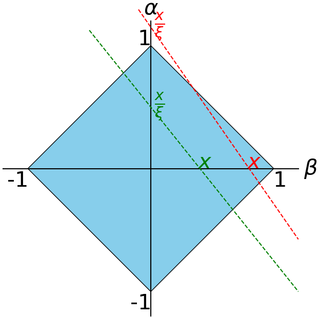
$\displaystyle\mathcal{R}$ $\displaystyle\longrightarrow$

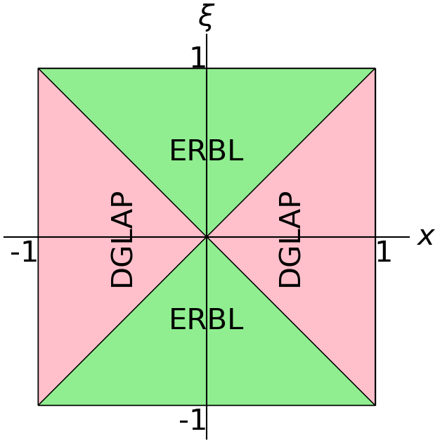
Figure 1: The domains $\Omega^{<}$ and $\Omega^{>}$ of the DD (resp. DGLAP and ERBL of the GPD) on the left (resp. right). The Radon transform $\mathcal{R}h\left(x,\xi\right)\propto\int\mathrm{d}\beta\mathrm{d}\alpha\,h(\beta,\alpha)\delta(x-\beta-\alpha\xi)$, which is an integration of $h$ on a line parameterized by the couple $(x,\xi)$, is the operation that sends one domain to the other. The goal of the inversion of the Radon transform is to rely only on DGLAP information, meaning that we have only access in DD space to integration lines that cross the $\alpha$ axis on $x/\xi>1$ (red lines). In this example, both $x$ and $\xi$ are positive.

Consider now a real $z$ such that $|z|>1$, i.e. $(0,z)\notin\Omega$. The families of straight lines joining $(0,z)$ to $(x,0)$ with $x\in]0,1]$ cover the whole domain $\Omega^{>}$. Thus any point in $\Omega^{>}$ contributes to DGLAP kinematics. If $|z|<1$, all points in the cone of apex $(0,z)$ and base delimited by $(0,0)$ and $(1-|z|,0)$ brings a contribution to the ERBL region. Proceeding with the limit $|z|\rightarrow 1^{-}$ we see that all points in $\Omega^{>}$ contribute to ERBL kinematics. The same discussion can of course be carried for $\Omega^{<}$. Therefore the entire DD support but the $\beta=0$ line is integrated over when $(x,\xi)$ covers the DGLAP or ERBL region. At this stage the question of the covariant extension of GPDs from the DGLAP to the ERBL region becomes to know whether it is possible to unravel an underlying DD $h(\beta,\alpha)$ or $F_{\textrm{PW}}(\beta,\alpha)$ on $\Omega$ uniquely from the DGLAP region.

III.2 Formalization

At the GPD level, a D-term $\delta(\beta)D(\alpha)$ is visible only in the ERBL region. At the DD level, a D-term is irrelevant in the geometric construction of the previous paragraph. There is a minimal ambiguity in the extension from the DGLAP to the ERBL region. Is it the only one?

In other words, assume there are two GPDs $H_{1}$ and $H_{2}$ which are equal over the DGLAP region. Are they equal over the ERBL region, up to a D-term? Without loss of generality, we can consider $H=H_{1}-H_{2}$ by linearity of the Radon transform. This $H$ is zero in the DGLAP region. Since this reasoning holds up to a D-term, we can express $H$ in the PW scheme assuming that $D_{\textrm{PW}}=0$. We want to show that $F_{\textrm{PW}}=0$. We will rely on the theorem of Boman and Todd Quinto mentioned in Sec. A. Switching to Radon transform canonical variables with Eqs. (14)-(15), the membership to the DGLAP and ERBL regions becomes:

$$(x,\xi)\in\textrm{ DGLAP} \Leftrightarrow |s|\geq|\sin\phi|\;,$$ (53)

$$(x,\xi)\in\textrm{ ERBL} \Leftrightarrow |s|\leq|\sin\phi|\;.$$ (54)

Note that $|\xi|\leq 1$ means $\phi\in[0,\pi/4]\cup[3\pi/4,5\pi/4]\cup[7\pi/4,2\pi]$. The complementary range in $[0,2\pi]$ corresponds to the physical domain of Generalized Distribution Amplitudes (GDAs) Mueller et al. (1994); Diehl et al. (1998, 2000) which are the crossed-channel analog of GPDs. In the DGLAP region, the GPD is zero if $|x|>1$, which is equivalent to $|s|>|\cos\phi|$, which is larger than $|\sin\phi|$ for $|\xi|<1$, i.e. in the GPD physical domain. We therefore assume here that:

$$H\left(\frac{s}{\cos\phi},\tan\phi\right)=0\quad\textrm{ for }s>\sin\phi\textrm{ and }\phi\in[0,\pi/4]\;.$$ (55)

Let us choose $\xi_{0}\in[0,1]$ and $x_{0}\in]\xi_{0},+\infty[$. We write $\tan\phi_{0}=\xi_{0}$ with $\phi_{0}\in[0,\pi/4]$ and take $s_{0}$ verifying $x_{0}\cos\phi_{0}>s_{0}>\sin\phi_{0}.$ By continuity of the $\sin$ function, there exists $\epsilon>0$ such that $s_{0}>\sin\phi$ for $|\phi-\phi_{0}|<\epsilon$. It follows that $\mathcal{R}F_{\textrm{PW}}\left(s,\phi\right)=0$ for $s>s_{0}$ and $\phi\in]\phi_{0}-\epsilon,\phi_{0}+\epsilon[$. The aforementioned theorem of Boman and Todd Quinto asserts that:

$$F_{\textrm{PW}}(\beta,\alpha)=0\quad\textrm{ for all }(\beta,\alpha)\in\Omega^{>}\textrm{ such that }\beta\cos\phi_{0}+\alpha\sin\phi_{0}=s>s_{0}\;.$$ (56)

Selecting $s=x_{0}\cos\phi_{0}$, this last condition implies:

$$F_{\textrm{PW}}(\beta,\alpha)=0\quad\textrm{ for all }(\beta,\alpha)\in\Omega^{>}\textrm{ such that }\beta+\alpha\xi_{0}=x_{0}\;.$$ (57)

Thus $F_{\textrm{PW}}$ vanishes on all lines contributing to the DGLAP region, i.e. $F_{\textrm{PW}}=0$ on $\Omega^{>}$. Therefore the knowledge of a GPD in the DGLAP region fully determines it over the whole physical domain up to terms inherited from DDs with support on the line $\beta=0$. This is completely consistent with the discussion about the D-term at the beginning of this section.

What is the manifestation at the GPD level of DDs with support on the line $\beta=0$? Assume we started from a function $H_{\textrm{source}}$ defined in the DGLAP region, and that we were able to identify one DD $F_{\textrm{PW}}$ in the PW scheme such that $H_{\textrm{source}}=\mathcal{R}F_{\textrm{PW}}$. Let us further assume that $F_{\textrm{PW}}$ is properly normalized, i.e. that it yields the correct valence quark number (from the PDF) or the correct electric charge (from the form factor at vanishing momentum transfer). If $F_{\textrm{PW}}$ is a function, its values along the line $\beta=0$ do not contribute to line integrals over $\Omega$ since this subset has measure 0. In this case there is no remaining freedom. If $F_{\textrm{PW}}$ is not a function, we already saw the D-term contribution. We cannot exclude a priori contributions like $\delta(\beta)D^{+}(\alpha)$ where $D^{+}$ is an even function. For $\xi>0$ this modifies $H$ by the addition of a term:

$$\delta_{F}H(x,\xi)=\frac{1}{\xi}D^{+}\left(\frac{x}{\xi}\right)\;.$$ (58)

If $\xi=0$, this new term manifests itself in the PDF through:

$$\delta_{F}H(x,0)=2\delta(x)\int_{0}^{1}\mathrm{d}\alpha D^{+}(\alpha)\;.$$ (59)

Such a term would violate quark number conservation if $\int_{0}^{1}\mathrm{d}\alpha D^{+}(\alpha)\neq 0$, but there does not seem to be any first principle reason to forbid such terms if this integral does indeed vanish. Such terms have already been considered e.g. in Ref. Radyushkin (1999). Generally speaking, we end up with two families of ambiguities at the DD level:

1. Modification of the DD $F$ on the line $\beta$ = 0: terms like $\delta(\beta)D^{+}(\alpha)$ where $D^{+}$ is even, has support in $[-1,+1]$ and has vanishing integral over $[0,1]$.

2. Modification of the DD $G$ on the line $\beta$ = 0: terms like $\delta(\beta)D^{-}(\alpha)$ where $D^{-}$ is odd and has support in $[-1,+1]$.

In principle, there could also exist ambiguities involving derivatives of the Dirac distribution, i.e. $\delta^{(n)}(\beta)D^{\pm}_{n}(\alpha)$. Line integrals of such terms contribute to the GPD $H$ with $1/(|\xi|\xi^{n})D_{n}^{(n)}(x/\xi)$ up to a factor $\xi$ depending on whether this term is attached to the DD $F$ (with $D^{+}_{n}$) or to the DD $G$ (with $D^{-}_{n}$). The presence of such terms does not change the argument of our discussion. Their phenomenological relevance will be discussed elsewhere, and we will stick to the $\delta(\beta)D^{\pm}(\alpha)$ ambiguities in the following.

Let us summarize: the knowledge of a GPD in the DGLAP region is enough to constrain it in the ERBL region up to additional terms like (for $\xi\in[-1,+1]$):

$$\delta H(x,\xi)=\frac{1}{|\xi|}D^{+}\left(\frac{x}{\xi}\right)+\operatorname{sgn}(\xi)D^{-}\left(\frac{x}{\xi}\right)\;.$$ (60)

These terms contribute only to the ERBL region. In other words, the inverse problem of reconstructing a GPD from its restriction to the DGLAP region admits infinitely many solutions. Two distinct solutions differ by $D^{+}$ and $D^{-}$ terms as in Eq. (60). This statement is independent of the choice of an underlying DD scheme.

The $D^{+}$ and $D^{-}$ terms modify the polynomiality relation (11) by acting on the two highest degree coefficients:

$$\int_{-1}^{+1}\mathrm{d}xx^{m}\delta H(x,\xi)=\left(\xi^{m}\int_{-1}^{+1}\mathrm{d}zz^{m}D^{+}(z)+\xi^{m+1}\int_{-1}^{+1}\mathrm{d}zz^{m}D^{-}(z)\right)\;.$$ (61)

Since $D^{+}$ and $D^{-}$ have opposite parities, the $F$- and $G$-terms do not simultaneously modify the polynomiality relation. To the best of our knowledge, the ambiguity linked to $F$-terms has not been discussed so far in this context.

III.3 Problem reduction

We have so far discussed that the overlap representation, as expressed by Eq. (II.1), makes sure the positivity of the GPD; that there is no simple way to exploit the overlap in the ERBL region and, for the same price, respect the polynomiality condition at any finite truncation order in Fock space; and, finally, that the DD representation ensures this polynomiality. Thus, an immediate and natural approach to model a GPD, by fulfilling both positivity and polynomiality conditions and exploiting the physical information encoded in the LFWFs would result from:

1. the computation of the overlap DGLAP GPD, symmetric in Fock space (overlap of LFWFs with the same number of constituents),

2. the derivation of a DD from this DGLAP GPD by an inverse problem,

3. the extension of the GPD to its full kinematic domain by means of the DD representation.

This is the program we will apply in the following.

In particular, given a GPD $H(x,\xi)$ with support $x\in[-1,+1]$ and with available non-trivial information only in the DGLAP region $0\leq\xi\leq|x|\leq 1$, our goal is to find a DD $h$ such that:

$$H(x,\xi) = C^{>}(x,\xi)\int_{\Omega^{>}}\mathrm{d}\beta\mathrm{d}\alpha\,h(\beta,\alpha)\,\delta(x-\beta-\alpha\xi)$$ (62)

$$+ C^{<}(x,\xi)\int_{\Omega^{<}}\mathrm{d}\beta\mathrm{d}\alpha\,h(\beta,\alpha)\,\delta(x-\beta-\alpha\xi)\;,$$

where the factors $C^{>}$ and $C^{<}$ were defined in Sec. II.2.3.

In the next section, we describe a well-established numerical procedure to do it. But before, we make the following remarks:

• The quark and anti-quark GPDs are not correlated in the DGLAP region. In positive DGLAP ($0\leq\xi\leq x$), only $H^{>}$ is present, while in negative DGLAP ($x\leq-\xi\leq 0$), only $H^{<}$ is. The two parts interfere in the ERBL region ($-\xi<x<\xi$) where $H=H^{>}+H^{<}$. Therefore, the task to accomplish is an independent inversion of Eq. (30) and Eq. (31).

• As mentioned in Sec. II.2, $h$ is $\alpha$-odd as the consequence of time reversal invariance.

These two properties together reduce the size of a numerical problem by $4$ by comparison of a direct numerical inversion of Eq. (62). Indeed, we can separate a general GPD into two distinct problems $H^{>}$ and $H^{<}$, by virtue of linearity of Eq. (62) and the non-correlation in the DGLAP region. This limits us to half the DD domain (either $\Omega^{>}$ or $\Omega^{<}$) without loss of generality. And by parity, we reduce again the problem by half. Figure 2 summarizes this. This significantly decreases the computing cost of the numerical inversion and further constrains the target solution.

As stated in Sec. II.2.3, we will discuss only the case of quark DDs and GPDs. The treatment of anti-quark DDs and GPDs is essentially the same.

$\displaystyle\mathcal{R}$ $\displaystyle\longrightarrow$

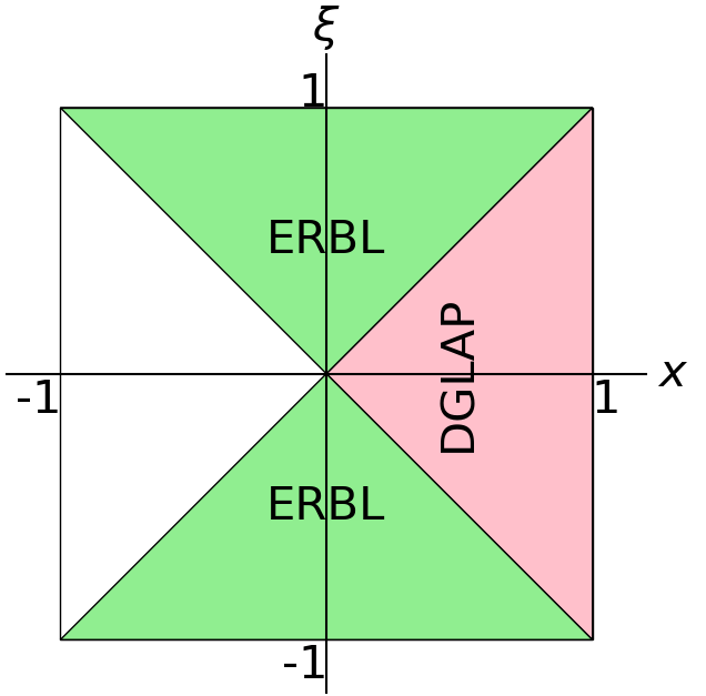
Figure 2: DD and GPD supports when only $\Omega^{>}$ is considered. Only the salmon red domain is used. The blue one is deduced by parity. And the white one, i.e. $\Omega^{<}$, is not correlated in DGLAP, and therefore can be dealt with separately.

IV Numerical implementation

This section presents the considered numerical implementation of the covariant extension of a GPD from the DGLAP to the ERBL region with its challenges and results. In Sec. III we explained that we can solve our physics problem by inverting the Radon transform. This may seem straightforward since the Radon transform is linear, but this task is in fact much more difficult. Indeed the inverse Radon transform may not be continuous (see App. A) and, in a loose sense, two “close” GPDs may be obtained as Radon transforms of very “different” DDs. Since we are facing an incomplete data problem (we know the GPD only in the DGLAP region), the sensitivity to noise is expected to be even stronger than in the complete data problem, where we search a DD from the complete knowledge of a GPD and a GDA over their whole kinematic domains. In this respect, we note that reconstruction artifacts have already been reported Teryaev (2001); Mezrag (2015) for the latter situation.

One key remark is in order here. We do not know any closed-form formula for the inverse of the Radon transform restricted to the DGLAP region. It is not even clear that such a formula even exists. However we do not need it, and it would be of limited practical interest: the potential amplification of noise is related to the discontinuous nature of the inverse Radon transform. It is not the manifestation of a poor numerical scheme or of a badly-designed computing code. It is the inescapable consequence of a precise and general mathematical statement. Even if we had at our disposal a closed-form expression of the inverse Radon transform, we should expect this phenomenon of noise amplification except in the lucky but rare situations where all computations can be performed analytically. As soon as approximations enter the game, the discontinuous nature of the inverse Radon transform may generate some artifacts in the sought-after DD.

The way to go is well-known in the mathematical literature (see e.g. Ref. Natterer (2001)). Assuming that the underlying DD is smooth enough, it is possible to numerically invert the Radon transform while keeping noise under control. This is called regularization.

This sections falls into three parts. We first discretize our problem to reduce it to the computation of the pseudo inverse of a rectangular matrix. Then we select adequate linear solver and regularization procedure. At last we validate our computing chain with simple but relevant test case scenarios.

IV.1 Discretization

The goal now is to obtain a discrete problem from the integral equation (30), and we will use the usual notation:

$$AX=B\,,$$ (63)

where $A$ is a $m\times n$ matrix, $X$ a vector of dimension $n$, and $B$ a vector of dimension $m$.

IV.1.1 Mesh

To obtain this finite-dimensional linear problem, the DD space should first be discretized. In an abstract way, we use a set of basis functions $\left\{v_{j}\right\}$ for the decomposition:

$$h\left(\beta,\alpha\right)=\sum_{j}h_{j}\,v_{j}\left(\beta,\alpha\right)\,,$$ (64)

where the index $j$ labels the set of basis functions, and therefore the degrees of freedom. Adopting a formalism close to the one of Finite Element Methods (FEM) Langtangen and Mardal (2016), these basis functions are in one-to-one correspondence to given nodes in the DD domain. Indexing these nodes means indexing the basis functions. Applying this to a given mesh which is a set of vertices (or corners) and edges defining its elements, we can be more explicit. A basis function is non-zero only on elements adjacent to its corresponding node, and the restriction of a basis function to one such element is the Lagrange interpolation with respect to this node, i.e. the polynomial that is equal to $1$ on the said node, and $0$ on all others. See Fig. 3 for an example of such a basis function.

Following the conventions of FEM Arnold and Logg (2014), we will consider the following classification:

$P_{n}$-Lagrange

Used for triangular meshes, where the restriction of a basis function to a triangular element is an interpolating polynomial of total degree at most $n$. For example, for $P_{1}$, it would be a polynomial of the form $a+b\,\beta+c\,\alpha$.

$Q_{n}$-Lagrange

Used for quadrilateral meshes, where the restriction of the basis function to a mesh element is an interpolating polynomial of partial degree at most $n$. For example, for $Q_{1}$, it would be a polynomial of the form $a+b\,\beta+c\,\alpha+d\,\beta\,\alpha$.

In the case of linear piece-wise functions ($P_{1}$ or $Q_{1}$), the considered nodes of the basis functions are the vertices of the mesh. For higher orders, the nodes also include other points (such as the middle of the edges for $P_{2}$ and $Q_{2}$). We will also consider constant piece-wise functions and we will call those elements $P_{0}$ (which corresponds to $dP_{0}$ in FEM notations). In this case, each basis function corresponds to one element (or any node in the interior of the element, e.g. the center of gravity, to keep the same correspondence between nodes and basis functions). Tab. 1 summarizes this.

Our unknowns $\left\{h_{j}\right\}$ of Eq. (64) correspond to the values of the DD $h$ on the nodes $j$, and will be recast into the vector $X$ of the discrete problem (63).

Order $n$	Basis function	Node
0	Piece-wise constant	Center of gravity of an element
1	Piece-wise linear	Vertex of the mesh
2	Piece-wise quadratic	Vertex or middle of an edge

Table 1: Summary of the different $P_{n}$ elements. Each basis function has support on the elements surrounding the corresponding node. The restriction to an element is a Lagrange interpolation: it takes a value of $1$ on the said node, and $0$ on all the other nodes.

For the work presented here, we will consider only a triangular mesh, since the domain is a triangle anyway (see Fig. 2), with $P_{1}$ or $P_{0}$ elements.

We will always use the index $j$ in the following to label the basis functions, i.e. the nodes, and the index $k$ for labelling the triangular elements. Of course, in the case of $P_{0}$, the indices will be interchangeable, since a basis function is defined by an element.

IV.1.2 Basis functions

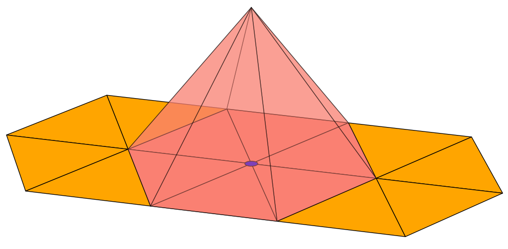
Figure 3: Example of a $P_{1}$ basis function. The corresponding node (i.e. a vertex in this case) is represented in blue. The value of the basis function on this node is 1, and 0 on the others. The support is limited to the adjacent triangles (in salmon red color).

In the case of a triangular mesh, it is natural to use barycentric coordinates to define the basis functions (instead of the Cartesian coordinates). For a given triangle $k$, we will denote by {$\lambda_{k}^{1}\left(\beta,\alpha\right)$, $\lambda_{k}^{2}\left(\beta,\alpha\right)$, $\lambda_{k}^{3}\left(\beta,\alpha\right)$} the barycentric coordinates with respect to the three vertices. Note that the number of degrees of freedom is still $2$, since ${\lambda_{k}^{1}+\lambda_{k}^{2}+\lambda_{k}^{3}=1}$. A given point $\left(\beta,\alpha\right)$ belongs to the triangle $k$ if all three barycentric coordinates are positive. Moreover, for $P_{1}$ elements, they provide natural restrictions for the basis functions, since they are exactly the linear Lagrange interpolations at the vertices. If we denote by $\left(\beta_{i},\alpha_{i}\right)$, $i=1\ldots 3$, the three vertices of a triangle, then the barycentric coefficient with respect to the first vertex can be written as:

$$\lambda^{1}\left(\beta,\alpha\right)=\frac{\beta_{3}\,\alpha_{2}-\beta_{2}\,\alpha_{3}+\left(\alpha_{3}-\alpha_{2}\right)\beta+\left(\beta_{2}-\beta_{3}\right)\alpha}{\beta_{3}\,\alpha_{2}-\beta_{2}\,\alpha_{3}+\left(\alpha_{3}-\alpha_{2}\right)\beta_{1}+\left(\beta_{2}-\beta_{3}\right)\alpha_{1}}\,,$$ (65)

and the others similarly by cycling indices.

The matrix of the linear problem is determined by the linear operator that transforms a DD into a GPD in Eq. (30). To build this matrix, we only need to know the Radon transform of a basis function:

$$\mathcal{R}v_{j}\left(x,\xi\right) = \int v_{j}\left(\beta,\alpha\right)\delta\left(x-\beta-\alpha\xi\right)\mathrm{d}\beta\,\mathrm{d}\alpha\,.$$ (66)

Let us first express this basis function in the $P_{0}$ and $P_{1}$ cases (superscripts 0 and 1 respectively):

$$v_{j}^{0}\left(\beta,\alpha\right) = \theta\left(\lambda_{j}^{1}\left(\beta,\alpha\right)\right)\,\theta\left(\lambda_{j}^{2}\left(\beta,\alpha\right)\right)\,\theta\left(\lambda_{j}^{3}\left(\beta,\alpha\right)\right)\,,$$ (67)

$$v_{j}^{1}\left(\beta,\alpha\right) = \sum_{\begin{subarray}{c}k\,\in\,\text{elements}\\ \text{adjacent to vertex }j\end{subarray}}\theta\left(\lambda_{k}^{1}\left(\beta,\alpha\right)\right)\,\theta\left(\lambda_{k}^{2}\left(\beta,\alpha\right)\right)\,\theta\left(\lambda_{k}^{3}\left(\beta,\alpha\right)\right)\,\lambda_{k}^{\bar{j}}\left(\beta,\alpha\right)\,,$$ (68)

where $\bar{j}$ is the vertex $j$ recast to the limited set $\left\{1,2,3\right\}$ of vertices of the element $k$. The $P_{1}$ basis function is also represented in Fig. 3. Applying the Radon transform on these basis functions yields:

$$\mathcal{R}v_{j}^{0}\left(x,\xi\right) = \theta\left(\alpha^{j}_{\text{max}}-\alpha^{j}_{\text{min}}\right)\left(\alpha^{j}_{\text{max}}-\alpha^{j}_{\text{min}}\right)\,,$$ (69)

$$\mathcal{R}v_{j}^{1}\left(x,\xi\right) = \sum_{\begin{subarray}{c}k\,\in\,\text{elements}\\ \text{adjacent to vertex }j\end{subarray}}\theta\left(\alpha^{k}_{\text{max}}-\alpha^{k}_{\text{min}}\right)\int_{\alpha^{k}_{\text{min}}}^{\alpha^{k}_{\text{max}}}\mathrm{d}\alpha\,\lambda_{k}^{\bar{j}}\left(x-\alpha\xi,\alpha\right)\,,$$ (70)

where the bounds of the integration $\left\{\alpha^{k}_{\text{min}},\alpha^{k}_{\text{max}}\right\}$ are determined with the three inequalities given by the Heaviside functions (positive barycentric coordinates). For higher order elements, the idea is the same, only the integrated function will change.

IV.1.3 Sampling

The next step is then to discretize the GPD variables $\left(x,\xi\right)$, i.e. to sample the set of straight lines intersecting the domain $\Omega$. Given that we have only access to DGLAP kinematics, we will use the couples $(x,y)\in[-1,+1]^{2}$ with $y=\xi/x$. The choice of $(x,y)$ will determine a line of the matrix. More precisely, the matrix $A$ will have the coefficients:

$$A_{ij}=C^{>}\left(x_{i},\xi_{i}\right)\,\mathcal{R}v_{j}\left(x_{i},\xi_{i}\right)\,,$$ (71)

where $1\leq i\leq m$ indexes the lines of the matrix, and $1\leq j\leq n$ indexes the columns, i.e. the nodes in DD space. The $C^{>}$ factor was introduced in Eq. (30).

The size of the matrix is chosen such that we maximize the information, i.e. we need to integrate over lines that cross all the elements of the DD mesh. A value of $m\sim 4\,n$ is empirically satisfying. The matrix can be therefore built by picking random couples $\left(x,y\right)$ until we attain the desired size. The results will of course depend on the matrix used and it is interesting to consider this as a source of “statistical error”, whereas the regularization procedure (see the following section) would be the source of “systematic error”. The statistical error can be managed quite easily and reduced considerably by picking as many samples as we want, whereas the systematic error remains a challenge to estimate.

Once the matrix is built, we use the set of chosen couples $\left(x,y\right)$ to build the vector $B$ r.h.s. of Eq. (63) with simply:

$$B_{i}=H^{>}\left(x_{i},\xi_{i}\right)\,.$$ (72)

In summary, $A$ is a matrix $m\times n$ where $n$ is the number of mesh elements for $P_{0}$ (or number of vertices for $P_{1}$) and $m$ the number of straight lines intersecting $\Omega$. Each line will typically cross $\mathcal{O}(\sqrt{n})$ mesh elements, which means that only $\mathcal{O}(\sqrt{n})$ coefficients on a matrix line are non-zero and $A$ is a sparse matrix. We need more constraints than parameters ($m>n$) and we usually use $m=4n$, making the rank of $A$ $\lesssim n$ (i.e. close to full-rank). $B$ is a vector of dimension $m$, and $X$ of dimension $n$.

IV.2 Linear solver and regularization

An additional complexity arises in the selection of the matrix inversion routine. In Sec. III.2 we assumed the existence of a covariant extension of a DGLAP-restricted GPD $H_{|\textrm{DGLAP}}$ and showed its uniqueness up to the manifestations of ambiguities on the line $\beta=0$. The key question is to know whether such an extension ever exist? Or, stated differently, given a function defined in the DGLAP region (a putative overlap of LFWFs), is it possible to extend it to the ERBL region in a way satisfying polynomiality? Existing criterions as in Eq. (42) and Eq. (44), complemented by the Ludwig-Helgason consistency conditions, deal with the GPD known over its whole physical domain, not its restriction to the DGLAP region. A numerical solver may have to handle a linear system as in Eq. (63) but without one and only one solution. This is common in computerized tomography, not because the solution does not exist (there was one object inserted inside the scanning device), but because the experimental signal comes with noise which may apparently modify the original situation to an inconsistent data problem. In the framework of the Radon transform, causes may be multiple: the integration lines may not cross the same domain (no solutions), or they may be parallel and close to one another and bring redundant information (infinitely many solutions). One efficient way to ensure that the solution always exists and is unique is to turn to a least-square formulation:

$$\textrm{Search }X\in\mathbb{R}^{n}\textrm{ such that }||AX-B||^{2}\textrm{ is minimum,}$$ (73)

where $||.||$ generically denotes a norm in a finite-dimensional vector space.

In the present work, we use a recent iterative conjugate-gradient type algorithm for sparse least-squares problems: LSMR Fong and Saunders (2010). For inconsistent problems (where the least-square formulation is favored), it is equivalent to a Minimum Residual algorithm for the problem:

$${}^{t}AA\,X={}^{t}AB\,,$$ (74)

but it can also solve directly the problem (63) when it is consistent, i.e. when the numerical approximation of the target solution is equal to the exact function. In the $P_{0}$ case, it means functions that are already piece-wise constant, whereas a $P_{1}$ approximation can reproduce exactly a (piece-wise) linear polynomial.

This type of algorithms applies naturally its own regularization process, with the number of iterations being the regularization parameter. To illustrate this, we can use the so-called L-curve Hansen (2007), which is a curve following a regularization parameter (which is in our case the number of iterations) and shows the compromise between the norm of the solution $\left\|X\right\|$ (the larger the norm, the larger the impact of noise) and the residual norm $\left\|r\right\|$, where $r=AX-B$ (which we desire to be small enough to converge to the real solution). This procedure gives the optimal regularization factor to choose for each problem, as the point of maximum curvature of the “L”, as shown in Fig. 4.

Figure 4: L-curve obtained with the number of iterations as regularization parameter for the case of Sec. V.1.

In practice, as illustrated on Fig. 4, it is very difficult to determine this optimal regularization parameter for the considered problems. A better way to stop the iterations is to consider the stopping criteria used by these algorithms such as LSMR:

• For a consistent problem: $\left\|r\right\|\leq\texttt{atol}\,\left\|A\right\|\,\left\|X\right\|+\texttt{btol}\,\left\|B\right\|$ ;

• For a least-squares problem: $\left\|A\,r\right\|\leq\texttt{atol}\,\left\|A\right\|\,\left\|r\right\|$,

where atol and btol are the input tolerances.

An empirical value of $10^{-5}$ for the least-square tolerances gives a good compromise between noise and convergence, and this has the benefit of being valid for all considered cases, assuming that the considered DD is smooth and not one of the problematic cases with singularities such as Sec. V.3 (for which a specific workaround is needed and explained therein). A $10^{-5}$ value for atol (resp. btol) means that the matrix $A$ (resp. the right hand side $B$) is known exactly up to the fifth decimal, while the rest is numerical noise. Of course, in practice, we can compute analytically $A$ (if the chosen basis functions and mesh allow us to compute the Radon Transform without numerical integration, as it is the case for the method presented here) and $B$ (if the GPD is known analytically), and they are therefore known exactly, up to machine precision. But in the inconsistent (i.e. least-squares) case, the considered vector $B$ is different from the one due to a GPD calculated from the discrete numerical DD. This difference is the finite limit of the residual, in contrast with the consistent case where the residual has a zero limit. Even though small, when allied with the ill-posed character of the inversion, it can have a large impact on the solution. This is why we consider in practice that $B$ (or equivalently $A$) is not known exactly and neglect higher decimals ; we apply a regularization procedure by doing so.

IV.3 Test and validation of the numerics

The first immediate check we can perform to validate the numerical implementation described above, consists in the following. We first take a simple Ansatz for the DD, irrespective of the considered value of $t$ (e.g. $t=0$). We then compute the associated analytical GPD by applying the Radon transform, and use only its DGLAP part to apply our numerical inversion and obtain a numerical estimate of the DD. Finally, we compare this result with the original Ansatz. We will apply this testing procedure to the following three quark GPDs, each one of them deriving from a DD in the P scheme:

• A constant DD $h_{p}^{\rm cst}(\beta,\alpha)$ on the half-domain $\Omega^{>}$:

  $$h_{\textrm{P}}^{\rm cst}(\beta,\alpha)=\frac{3}{2}\theta(\beta)\ \ \ \Rightarrow\ \ \ H(x,\xi)=\frac{3(1-x)^{2}}{1-\xi^{2}}\;,$$ (75)

• the example defined by Eq. (160) and already introduced in Sec. II.2.4,

• and a simplified case of the RDDA:

  $$h_{\textrm{P}}^{\rm RDDA}(\beta,\alpha)=\frac{\Gamma(N+3/2)}{\sqrt{\pi}\,\Gamma(N+1)}\frac{\left[(1-\beta)^{2}-\alpha^{2}\right)^{N}}{\left(1-\beta\right)^{2N+1}}\frac{q(\beta)}{1-\beta}\;,$$ (76)

  where $q(\beta)$ is the associated PDF. In particular, we specialize for the case $N=1$ and take $q(\beta)=30\,\beta^{2}(1-\beta)^{2}$. We thus obtain a closed algebraic formula for the GPD which, in turn, can be numerically inverted with the procedure described above.

Figure 5: Comparison between algebraic, given by Eq. (75), and numerical results for $h_{\textrm{P}}^{\rm cst}(\beta,\alpha)$ at fixed values of $\alpha=\left[0,0.25,0.5,0.75\right]$ (left panel) and the corresponding GPD at fixed values of $\xi=\left[0,0.5,1\right]$ (right panel) for the case (i). The blue solid curves display the numerical results while the red dashed ones show the algebraic results. The black dotted curve indicate either the line $\beta+\alpha=1$ (left panel) or $x\pm\xi=0$ (right panel). The upper panel stands for a discretization obtained with $P_{0}$ elements, while the lower panel displays the results with $P_{1}$ elements.

Figure 6: Comparison between algebraic, given by Eq. (160), and numerical results for $h_{\textrm{P}}^{\textrm{Toy}}(\beta,\alpha)$ (left panel) and the corresponding GPD (right panel) for the case (ii). Same conventions as in Fig. 5.

Figure 7: Comparison between algebraic, given by Eq. (76), and numerical results for $h_{\textrm{P}}^{\rm{RDDA}}(\beta,\alpha)$ (left panel) and the corresponding GPD (right panel) for the case (iii). Same conventions as in Fig. 5.

In all cases, we adopted the P scheme as it appears to be a convenient representation for GPD models derived through a covariant extension of an overlap of LFWFs, as discussed in Sec. II. Therefore it will systematically be employed for the analysis of the more practical examples scrutinized in the next section. In the leftmost plots of Fig. 5, we display the comparison of the exact algebraic and numerically approximated $h_{\textrm{P}}^{\rm cst}(\beta,\alpha)$ for the case (i), while the rightmost ones stand for the comparison of the GPDs directly obtained from both DDs. The upper and lower plots have been obtained, respectively, with piecewise constant (i.e. $P_{0}$ elements) and piecewise linear (i.e. $P_{1}$) basis functions when discretizing the DD space for the reduction to a finite-dimensional problem, as explained in Sec. IV.1. Analogous plots, and similarly arranged, are displayed in Fig. 6 for case (ii) and Fig. 7 for case (iii).

The mesh was generated using the Triangle software Shewchuk (1996) with a requirement of maximal area for the triangular elements equal to $0.001$, which produced a mesh of $427$ vertices and $780$ elements. The linear solver used is described in Sec. IV.2. As justified before, we used a tolerance of $10^{-5}$ as a regularization procedure.

All in all, as an overall conclusion we can assert that the numerical inversion approximates very well the three known GPDs as they appear not to differ significantly in all the cases. Several important points should be however stressed out:

• The numerical inversion relies only on the knowledge of the GPD within the DGLAP region and its extension to the ERBL is our main goal, wherefore the examination of algebraic and numeric GPDs over the ERBL region is the main outcome of Figs. 5-7.

• The numerical reconstruction of the DDs may seem quite noisy or far off in some cases, but these discrepancies do not hinder the reconstruction of the GPD, for which the convolution helps smooth these defaults. The physical object of interest is the GPD, not the DD, therefore these discrepancies are not an issue.

• It should be noted however that the constant DD can be reconstructed numerically exactly (up to machine precision). Indeed, the regularization in that case is not needed, since there is no distinction between the analytical DD and its discretized version. We could therefore directly invert the discrete problem and recover the exact DD (which would be equivalent to using a tolerance of $0$ instead of $10^{-5}$), but for the sake of homogeneity, we decided to employ the same method for all shown examples.

• It may seem from the plots that the $P_{1}$ discretization does not improve on the $P_{0}$ result, but this is not true. We chose here to use the same mesh for both $P_{0}$ and $P_{1}$ elements. This particular mesh has $427$ vertices and $780$ triangular elements. Hence, the number of degrees of freedom for $P_{1}$ (i.e. the number of vertices) is half the one for $P_{0}$ (i.e. number of elements). In other words, we attain with $P_{1}$ a similar result to the $P_{0}$ one but with half the degrees of freedom, i.e. at a much lower cost. It is therefore a significant improvement. In Sec. V, we will keep only the $P_{1}$ method for non-trivial applications with popular LFWFs occurring in realistic descriptions of hadron structure.

V Examples of Applications

The approach described in Sec. II and Sec. III can be either applied to numerous existing LFWF-based GPD models to covariantly extend them from the DGLAP region to the ERBL one, or used to build a covariant GPD model, reliable on both DGLAP and ERBL regions, from the knowledge of the LFWF. Although in some particular cases, an analytical derivation of the DD is possible and a full GPD in both DGLAP and ERBL regions can be thereupon obtained, one can only proceed systematically by applying the numerical technique that has been introduced in section IV. In this section, aiming to illustrate the procedure without the intention of being exhaustive, we provide four examples of GPD models, three of which can be extended to the ERBL region both analytically and numerically, allowing us to benchmark our algorithm.

V.1 Algebraic Bethe-Salpeter model

We consider first a specific pion GPD model described in Ref. Mezrag et al. (2016), based on the following helicity-0:

$$\Psi_{l=0}\left(x,\textbf{k}_{\perp}\right)=8\,\sqrt{15}\,\pi\,\frac{M^{3}}{\left(\textbf{k}_{\perp}^{2}+M^{2}\right)^{2}}\,\left(1-x\right)x\,,$$ (77)

and helicity-1:

$$i\,k_{\perp}^{j}\,\Psi_{l=1}\left(x,\textbf{k}_{\perp}\right)=8\,\sqrt{15}\,\pi\,\frac{k_{\perp}^{j}\,M^{2}}{\left(\textbf{k}_{\perp}^{2}+M^{2}\right)^{2}}\,\left(1-x\right)x\,,\qquad j=1,2\,,$$ (78)

contributions to the LFWF, obtained by integrating and properly projecting the pion Bethe-Salpeter wave function resulting from the algebraic model described in Chang et al. (2013) where $M$ is a model mass parameter introduced at the level of the quark propagator. A value of $M\sim 0.318~{}$ allows to recover the pion charge radius Amendolia et al. (1986). Eqs. (77)-(78) correspond to specializing the helicity-0 and helicity-1 components given, respectively, by Eqs. (154) and (155) in Ref. Mezrag et al. (2016) for the asymptotic case $\nu=1$ therein. Then, exploiting the GPD overlap representation as described in Sec. II.1 and extending Eq. (9) with the two contributions:

$$H_{\pi^{+}}^{u}\left(x,\xi,t\right)=\int\frac{\mathrm{d}^{2}\mathbf{k}_{\bot}}{16\,\pi^{3}}\left[\Psi_{l=0}^{*}\left(\hat{x}^{{}^{\prime}},\hat{\mathbf{k}}_{\bot}^{{}^{\prime}}\right)\Psi_{l=0}\left(\tilde{x},\tilde{\mathbf{k}}_{\bot}\right)+\hat{\mathbf{k}}_{\bot}^{{}^{\prime}}\cdot\tilde{\mathbf{k}}_{\bot}\Psi_{l=1}^{*}\left(\hat{x}^{{}^{\prime}},\hat{\mathbf{k}}_{\bot}^{{}^{\prime}}\right)\Psi_{l=1}\left(\tilde{x},\tilde{\mathbf{k}}_{\bot}\right)\right]\,,$$ (79)

one is left with:

$$\left.H_{\pi^{+}}^{u}(x,\xi,t)\right|_{\xi\leq x}\ =\ \frac{15}{2}\ \frac{(1-x)^{2}(x^{2}-\xi^{2})}{(1-\xi^{2})^{2}}\ \frac{1}{(1+\zeta)^{2}}\left(3+\frac{1-2\zeta}{1+\zeta}\ \frac{\displaystyle\operatorname{arctanh}{\left(\sqrt{\frac{\zeta}{1+\zeta}}\right)}}{\displaystyle\sqrt{\frac{\zeta}{1+\zeta}}}\right)\ ,$$ (80)

as a fully algebraic result for the DGLAP region, where:

$$\zeta\ =\ \frac{-t}{4M^{2}}\frac{(1-x)^{2}}{1-\xi^{2}}\;,$$ (81)

encodes the correlated dependence of the kinematical variables $x$ and $t$.

Figure 8: Comparison between algebraic and numerical results for the pion GPD modeled in Ref. Mezrag et al. (2016). As it was the case in Fig. 5, the blue solid curves display the numerical results while the red dashed ones show the results algebraically derived and given by Eqs. (80)-(83). The left panel stands for the case $t=0$ for fixed values of $\xi=\left[0,0.5,1\right]$ and the right one shows the $t$-behavior for fixed values $\left[0,-0.25,-0.5\right]$ at $\xi=0.5$. We retain only $P_{1}$ elements. For more details, see Sec. IV.3.

A careful computation allows for the derivation of the following closed expression for the DD in the P scheme given by Eqs. (26)-(27):

$$h_{\textrm{P}}(\beta,\alpha,t)=\frac{15}{2}\frac{1-3\alpha^{2}-2\beta+3\beta^{2}+\frac{-t}{4M^{2}}\left(1-\alpha^{4}+2\alpha^{2}\beta^{2}-\beta^{4}+4\beta^{2}-4\beta\right)}{\left(1+\frac{-t}{4M^{2}}\left(\left(1-\beta\right)^{2}-\alpha^{2}\right)\right)^{3}}\theta(\beta)\;.$$ (82)

This last result then can be applied, as explained in Sec. III, to provide us with a covariant extension of the result given in Eq. (80) to the ERBL kinematic domain. A thorough scrutiny of the main features resulting from the pion GPD model of Ref. Mezrag et al. (2016) will be the object of a further work, in particular the study of the evolution in $t$ and its implications. However, the main purpose of bringing here this model computation is to benchmark the numerical technique developed in Sec. IV. This can be easily done, without any loss of generality, by focusing on the case $t=0$, for which one can write down, invoking Eq. (30), the following simple expression for the GPD within the ERBL domain:

$$\left.H_{\pi^{+}}^{u}(x,\xi,0)\right|_{|x|\leq\xi}\ =\ \frac{15}{2}\frac{(1-x)(\xi^{2}-x^{2})}{\xi^{3}(1+\xi)^{2}}\left(x+2x\xi+\xi^{2}\right)\ .$$ (83)

Thus, we compare the results given by Eq. (80) and Eq. (83), respectively derived for the DGLAP and ERBL kinematics, with those obtained by the numerical inversion of the linear problem described in section IV; and display the outcome in the leftmost panels of Fig. 8. As can be seen, both numerical and algebraic results compare strikingly well, not only at a qualitative but also a quantitative level. Albeit the successful comparison we obtain for the case $t=0$ is satisfactorily enough, aiming at the practical validation of the numerical technique at other values of $t$, we have also displayed in the rightmost panel of Fig. 8 the results for the GPD evolved in $t$ at a constant value of $\xi=0.5$. The algebraic expression for the DGLAP region is given in Eq. (80), while that for ERBL can be obtained by the integration of Eq. (82) through Eq. (30). The algebraic expression for the DGLAP region is given in Eq. (80), while that for ERBL can be obtained by the integration of Eq. (82).

V.2 Algebraic spectator model

If LFWFs have been widely used in attempts to model the pion, the case of the nucleon has also been treated previously, in particular in the pioneering paper of Hwang and Müller Hwang and Mueller (2008). They have developed an algebraic parametrization for two-body LFWFs of the nucleon (described by a constituent quark and a spectator scalar diquark):

$$\Psi_{+1/2}^{\uparrow}\left(x,\textbf{k}_{\perp}\right) = \Psi_{-1/2}^{\downarrow}\left(x,\textbf{k}_{\perp}\right)=\left(M+\frac{m}{X}\right)\varphi(x,\textbf{k}_{\perp}),$$ (84)

$$\Psi_{-1/2}^{\uparrow}\left(x,\textbf{k}_{\perp}\right) = -\frac{k^{1}+ik^{2}}{x}\varphi(x,\textbf{k}_{\perp}),\quad\Psi_{+1/2}^{\downarrow}\left(x,\textbf{k}_{\perp}\right)=\frac{k^{1}-ik^{2}}{x}\varphi(x,\textbf{k}_{\perp}),$$ (85)

$$\varphi(x,\textbf{k}_{\perp}) = \frac{gM^{2p}}{\sqrt{1-x}}x^{-p}\left(M^{2}-\frac{\textbf{k}_{\perp}^{2}+m^{2}}{x}-\frac{\textbf{k}_{\perp}^{2}+\lambda^{2}}{1-x}\right)^{-p-1},$$ (86)

with $M$, $m$ and $\lambda$ being respectively the nucleon, quark and spectator masses, $p$ being a free parameter. The authors have shown that with such a model, after calculating the overlap of wave functions (see Eqs. (13-14) of Ref. Hwang and Mueller (2008)), one can write the GPD $E$ in the P scheme:

$$E(x,\xi,t)=(1-x)\int_{0}^{1}\textrm{d}\beta\int_{-1+\beta}^{1-\beta}\textrm{d}\alpha\ e(\beta,\alpha,t)\,\delta(x-\beta-\xi\alpha),$$ (87)

and they have been able to extract analytically:

$$e\left(\beta,\alpha,t\right)=\frac{N\,\left(\beta+\frac{m}{M}\right)\left((1-\beta)^{2}-\alpha^{2}\right)^{p}}{\left(2\left(\frac{(1-\beta)m^{2}}{M^{2}}+\frac{\beta\lambda^{2}}{M^{2}}-(1-\beta)\beta-\frac{t\left((1-\beta)^{2}-\alpha^{2}\right)}{4M^{2}}\right)\right)^{2p+1}}$$ (88)

where $N$ is a constant determined by the usual PDF normalization (obtained with the GPD H, and not E). Therefore, the authors managed to extend their specific model in the ERBL region. Consequently, we use this model as an additional benchmark for our numerical technique.

The comparison between our numerical reconstruction and the algebraic result is shown on Fig. 9. We use the same parameters values as in Ref. Hwang and Mueller (2008), i.e. $M=1~{}$, $m=0.45~{}$, $\lambda=0.75~{}$ and $p=1$. In this case, the normalization constant for the DD is $N\sim 0.176$. We stress that in Fig. 9, the qualifying terms “analytical” and ”numerical” refer to the DDs. In other words, “analytical result” means that the GPD is calculated through an integration of the “analytical” DD (88) in the ERBL region (or through the integration of Eq. (15) in Ref. Hwang and Mueller (2008) in the DGLAP region), whereas “numerical result” means that the GPD is calculated from the ”numerically” reconstructed DD (from DGLAP information only), through e.g. Eqs. (64), (70) and (87).

Figure 9: Comparison for the GPD E between our numerical algorithm and the algebraic result of Ref. Hwang and Mueller (2008). Same conventions as in Fig. 8.

V.3 Parametrization with Regge behabior

All the previous examples dealt with GPDs smoothly behaving at $x=0$. However, phenomenological models for valence quark GPDs often exhibit an integrable singularity, typically a $1/\sqrt{x}$ behavior. If such a GPD is related to a DD $h_{\textrm{P}}$ in the P scheme, then it can be shown that $H(x,0)\sim\int_{-1}^{+1}\mathrm{d}\alpha\,h_{\textrm{P}}(x,\alpha)$ at small $x$. Therefore $h_{\textrm{P}}$ itself may also exhibit an integrable singularity $1/\sqrt{\beta}$. The numerical method presented up to now approximates the target DD by piecewise constant or piecewise linear functions on $\Omega$. In particular all approximations are bounded, even if in principle they can be more and more peaked when the mesh gets thinner. As discussed in Sec. IV, careful choices of the size of the mesh and of the number of iterations are essential for the resolution of the inverse problem with adequate control of the numerical noise. With a naive discretization, it is difficult when dealing with singularities to make sense of a solution ; it would probably require a number of iterations that is not attainable due to the necessary truncation of the regularization. We thus adopt a more educated discretization ; knowing that we are dealing with Regge-type singularities, we can adapt our method accordingly, by discretizing:

$$h_{\textrm{P}}^{\prime}(\beta,\alpha)=\sqrt{\beta}\ h_{\textrm{P}}(\beta,\alpha)$$ (89)

which will be less singular that $h_{\textrm{P}}$, possibly even free of singularities. This change of target function only modifies the kernel of Eq. (30) (it is not a Radon transform anymore), otherwise everything readily follows the same procedure.

Figure 10: Comparison between algebraic and numerical results for the GPD corresponding to the model of Eq. (91). Same conventions as in Fig. 8 (left panel).

Let us exemplify this technique on a simple parameterization of nucleon DD for which, once again, the expression is already known. We use the RDDA as presented in Sec. IV.3, Eq. (76) for $N=1$, but this time with a singular PDF:

$$q_{\textrm{Regge}}\left(x\right)=\frac{35\ (1-x)^{3}}{32\ \sqrt{x}}\ ,$$ (90)

which would give the following DD (with a $1/\sqrt{\beta}$ singularity) on $\Omega^{>}$:

$$h_{p}^{\textrm{Regge}}\left(\beta,\alpha\right)=\frac{105\left(\alpha^{2}-\left(\beta-1\right)^{2}\right)}{128\ \left(\beta-1\right)\sqrt{\beta}}\ .$$ (91)

The comparison between the algebraic GPD and the result obtained through the numerical reconstruction of the DD with DGLAP information is shown on Fig. 10.

V.4 Gaussian wave functions

Figure 11: Results obtained for the GPD $H$ in the case of a Gaussian LFWF. Same conventions as in Fig. 8, but without analytical benchmark.

Last, on top of the Bethe-Salpeter wave function already mentioned above in the pion case, one can compute a LFWF with a Gaussian Ansatz (such Ansätze have been used for instance in ADS/QCD computations, see Ref. Brodsky et al. (2015) and refs therein). We choose to work with the following one:

$$\Psi\left(x,\mathbf{k}_{\perp}^{2}\right)=\frac{4\sqrt{15}\,\pi}{M}\,\sqrt{x\,(1-x)}\,e^{-\frac{\mathbf{k}_{\perp}^{2}}{4M^{2}(1-x)x}}\,.$$ (92)

This wave function yields in the DGLAP region (using Eq. (9)):

$$H\left(x,\xi,t\right)=\frac{30(x-1)^{2}\left(x^{2}-\xi^{2}\right)^{3/2}\exp\left(\frac{\left(1-\xi^{2}\right)t(1-x)}{8M^{2}\left(\xi^{2}(x-2)+x\right)}\right)}{\left(1-\xi^{2}\right)\left(-2\xi^{2}+\xi^{2}x+x\right)}\,.$$ (93)

To the best of our knowledge, an algebraic expression for the associated DD (it it exists) has not been published yet. We anyhow examine this case for illustrative purposes and display in Fig. 11 the results for the GPD in both DGLAP and ERBL derived from the DDs obtained with our numerical inversion. Indeed, some qualitative similarities in the shape can be noticed when compared to the results previously obtained with the Bethe-Salpeter LFWF and depicted in Fig. 8. The parameter value of $M\sim 0.315~{}$ has been used here.

VI Discussion

VI.1 Chiral symmetry and the soft pion theorem

Pion GPDs should satisfy one extra first principle constraint, tied to the specific role of the pion with respect to chiral symmetry. The isosinglet and isovector pion GPDs $H^{I=0}$ and $H^{I=1}$ are defined in terms of the following matrix elements:

$$\left\{\begin{array}[]{c}\delta^{ab}H^{I=0}(x,\xi,t)\\ i\epsilon^{abc}H^{I=1}(x,\xi,t)\end{array}\right. = \frac{1}{2}\int\frac{\mathrm{d}z^{-}}{2\pi}\,e^{ixP^{+}z^{-}}$$ (96)

$$\times \left\langle\pi^{b},P+\frac{\Delta}{2}\right|\bar{\Psi}\left(-\frac{z}{2}\right)\left\{\begin{array}[]{c}\mathcal{I}\gamma^{+}\\ \tau^{c}\gamma^{+}\end{array}\right\}\left[-\frac{z}{2};\frac{z}{2}\right]\Psi\left(\frac{z}{2}\right)\left|\pi^{a},P-\frac{\Delta}{2}\right\rangle_{z^{+}=0,z_{\perp}=0}\ ,$$ (99)

where $\Psi=(\psi^{u},\psi^{d})$ denotes the doublet of $u$ and $d$ quark fields, $\mathcal{I}$ is the identity, $\tau^{c}$ the Pauli matrices, $\tau^{\pm}=(\tau^{1}\pm i\tau^{2})/\sqrt{2}$, and $\left|\pi^{1}\right\rangle$, $\left|\pi^{2}\right\rangle$ and $\left|\pi^{3}\right\rangle$ is a basis of the adjoint representation of the Lie algebra $\mathfrak{su}(2)$. Expressing theses vectors in terms of charge eigenstates:

$$\left|\pi^{\pm}\right\rangle = \frac{1}{\sqrt{2}}\left(\left|\pi^{1}\right\rangle\pm i\left|\pi^{2}\right\rangle\right)\;,$$ (100)

$$\left|\pi^{0}\right\rangle = \left|\pi^{3}\right\rangle\;,$$ (101)

yields in particular:

$$H^{I=0}(x,\xi,t) = H^{u}_{\pi^{+}}(x,\xi,t)+H^{d}_{\pi^{+}}(x,\xi,t)\;,$$ (102)

$$= H^{u}_{\pi^{-}}(x,\xi,t)+H^{d}_{\pi^{-}}(x,\xi,t)\;,$$ (103)

$$H^{I=1}(x,\xi,t) = H^{u}_{\pi^{+}}(x,\xi,t)-H^{d}_{\pi^{+}}(x,\xi,t)\;.$$ (104)

$$= -H^{u}_{\pi^{-}}(x,\xi,t)+H^{d}_{\pi^{-}}(x,\xi,t)\;,$$ (105)

The additional charge conjugation constraint, $H^{q}_{\pi^{+}}(x,\xi,t)=-H^{q}_{\pi^{-}}(-x,\xi,t)$ for $q=u,d$ dictates:

$$H^{u}_{\pi^{+}}(x,\xi,t)=-H^{d}_{\pi^{+}}(-x,\xi,t)\;.$$ (106)

Therefore the information for the whole system of pion GPDs can be equivalently encoded in $H^{I=0}$ and $H^{I=1}$, or $H^{u}_{\pi^{+}}$ and $H^{d}_{\pi^{+}}$, which makes $H^{I=0}$ (resp. $H^{I=1}$) an odd (resp. even) function of $x$:

$$H^{I}(-x,\xi,t)=(-1)^{1-I}H^{I}(x,\xi,t)\quad\textrm{for}\quad I=0,1\;.$$ (107)

In the chiral limit, the soft pion theorem Polyakov (1999) states that:

$$H^{I=0}(x,\xi=1,t=0) = 0\;,$$ (108)

$$H^{I=1}(x,\xi=1,t=0) = \varphi_{\pi}\left(\frac{1+x}{2}\right)\;,$$ (109)

where $\varphi_{\pi}$ is the leading-twist pion DA. This theorem holds in any framework where chiral symmetry is properly implemented, as clearly exemplified in a recent independent derivation in the Dyson-Schwinger-Bethe-Salpeter framework Mezrag et al. (2014).

We saw in Sec. III.2 that an overlap of LFWFs in the DGLAP region characterizes a set of GPDs of the form:

$$H(x,\xi)=H_{\textrm{LFWF}}(x,\xi)+\delta H(x,\xi)\;,$$ (110)

with $\delta H$ defined in Eq. (60) and $H_{\textrm{LFWF}}(x,\xi)$ obtained from a numerical inversion of the Radon transform in a particular DD scheme. By linearity, this relation holds in a flavor basis or in an isospin basis. In particular, the $x$-parity of $D^{+}$ and $D^{-}$ induces two different contributions to the isoscalar and isovector GPDs, and hence to the soft pion theorem:

$$\big{(}D^{u-}+D^{d-}\big{)}(x,t=0) = -H_{\textrm{LFWF}}^{I=0}(x,\xi=1,t=0)\;,$$ (111)

$$\big{(}D^{u+}-D^{d+}\big{)}(x,t=0) = -H_{\textrm{LFWF}}^{I=1}(x,\xi=1,t=0)+\varphi_{\pi}\left(\frac{1+x}{2}\right)\;.$$ (112)

The requirement $\int\mathrm{d}zD^{+}(z)=0$ is manifest in this last equation. The normalization of the LFWFs used in the overlap leading to $H_{\textrm{LFWF}}$ imposes the equality of the form factor at vanishing momentum transfer and of the integral of the leading twist DA. Therefore the remaining freedom in the covariant extension of a GPD from the DGLAP to the ERBL region is flexible enough to satisfy the soft pion theorem. The latter is explicitly shown by a more detailed analysis of the algebraic Bethe-Salpeter model in Ref. Chouika et al. (2017).

We already emphasized that, for any hadron, our model building strategy systematically produces GPDs satisfying a priori polynomiality, positivity, and the correct consequences of discrete symmetries. We have just shown that, in the pion case, the soft pion theorem can always be fulfilled too. Whatever the input overlap is, we can construct a model obeying a priori all the first principles constraints. The reduction formulas to obtain PDFs or form factors impose further restrictions on the choice of the LFWFs –which can be read from the overlap in the DGLAP region– and not on the covariant extension in itself.

At last, to the best of our knowledge, nothing prevents the soft pion theorem to be satisfied in a model with an inadequate chiral symmetry behavior. Fulfilling the soft pion theorem may not be equivalent to enjoying a proper implementation of chiral symmetry breaking. However it is tantalizing to think that the soft pion theorem can only be met if the underlying LFWFs do possess a correct chiral behavior, in which case we may speculate about the physics content of the $D^{-}$ and $D^{+}$ terms restoring this chiral property. These considerations go beyond the scope of the present paper, and are left to a later study.

VI.2 Double Distributions: smoothness assumptions and schemes

The discussion of Sec. III.2 relied on the PW scheme, while the numerical examples of Sec. V involved the P scheme. From Eqs. (49)-(51), it is manifest that the numerical resolution can be straightforwardly adapted from one DD scheme to the other. However, even if the underlying physics (the GPD itself) is invariant under the change of DD schemes, choosing one particular DD scheme may have a practical impact in actual GPD computations. This is reminiscent of what is well-known about Green functions and Feynman diagrams in gauge field theories or kinematics in special relativity. Therefore we may wonder what is the impact of a DD scheme choice in the actual covariant extension of a GPD from the DGLAP to the ERBL region. Due to the prefactors relating $H$ and the Radon transforms of DDs in Eqs. (49)-(51), we may expect that different DD schemes will yield different GPD covariant extensions starting from the same GPD in the DGLAP region. This may give a feeling of arbitrariness of the result. On the contrary we will show below that the set of solutions of the inverse problem does not change. Whatever the choice of the DD scheme underlying the inverse of the Radon transform, given an input function in the DGLAP region, the set of GPDs whose restriction to the DGLAP region is this input function stays the same.

To prove this, we only need to study the influence of a DD scheme transformation on the set of solutions described in Sec. III.2 in the PW scheme, and in particular exhibit the manifestation of the $D^{+}$ and $D^{-}$ ambiguities in the BMKS and P schemes. Since DD scheme transformations are linear, we only have to adapt the general expressions given in App. B to the particular case:

$$F(\beta,\alpha) = \delta(\beta)D^{+}(\alpha)\;,$$ (113)

$$G(\beta,\alpha) = \delta(\beta)D^{-}(\alpha)\;.$$ (114)

Using Eq. (144), we see that the $D^{+}$ and $D^{-}$ ambiguities in the PW scheme bring a contribution $\delta h_{\textrm{P}}$ to the DD $h_{\textrm{P}}$ we would obtain by inverting the Radon transform in the P scheme:

$$\delta h_{\textrm{P}}(\beta,\alpha)=\delta(\beta)D^{+}(\alpha)+\frac{\theta(\beta)}{(1-\beta)^{2}}\bar{D}^{\prime}\left(\frac{\alpha}{1-\beta}\right)\;,$$ (115)

where $\bar{D}(z)=zD^{+}(z)+D^{-}(z)$. The corresponding exercise in the BMKS scheme yields:

$$\delta h_{\textrm{BMKS}}(\beta,\alpha)=\delta(\beta)\frac{D^{-}(\alpha)}{\alpha}-\delta^{\prime}(\beta)\int_{1}^{\alpha}\mathrm{d}\sigma\frac{D^{+}(\sigma)}{\sigma}\;.$$ (116)

Direct computations of the associated GPD contribution $\delta H$ establish that we actually recover the expression (60) derived in the PW scheme. The manifestation of the ambiguities related to $D^{+}$ and $D^{-}$ nevertheless presents different forms in different DD schemes.

We will now explain with the simple example $H^{\textrm{Toy}}$ of Eqs. (34)-(35) the impact of the different DD schemes we have considered so far. This GPD model was defined in the BMKS scheme from Eq. (32). As mentioned in Sec. II.2.6 it satisfies the necessary and sufficient condition (42) expressing its membership to the range of the Radon transform of summable functions in the BMKS scheme. We can express this GPD in the P scheme by means of Eq. (145) to obtain a DD $h_{\textrm{P}}^{\textrm{Toy}}$ which is not summable over $\Omega$ and violates the analogous necessary and sufficient condition (44) in the P scheme.

At the same time, we can numerically invert the Radon transform in the P scheme with the restriction $H_{|\textrm{DGLAP}}^{\textrm{Toy}}$ to the DGLAP region as an input function. The numerical procedure described in Sec. IV will approximate the DD in the P scheme by a piecewise linear function, and will naturally pick up a (reasonably) smooth solution among all the solutions of this inverse problem. This is indeed what has been successfully checked and showed in Fig. 6 with the second test case of Sec. IV.3. The DD $h_{\textrm{P, Reg}}^{\textrm{Toy}}$ (160) in the P scheme is smooth (it is a polynomial over $\Omega^{>}$), and is associated to a GPD equal in the DGLAP region to $H_{|\textrm{DGLAP}}^{\textrm{Toy}}$, which was derived from the original DD $h_{\textrm{BMKS}}^{\textrm{Toy}}$ in the BMKS scheme or its scheme-transformed partner $h_{\textrm{P}}^{\textrm{Toy}}$ (see Eqs. (161)-(162)). The P scheme DD $h_{\textrm{P, Reg}}^{\textrm{Toy}}$ defines a GPD model $H^{\textrm{Toy, Reg}}$ which is smooth enough to fulfill the necessary and sufficient condition (44) as explicitly evaluated in Eq. (48).

The two GPD models $H^{\textrm{Toy}}$ and $H^{\textrm{Toy, Reg}}$ differ only in the ERBL region by a $D^{-}$-type contribution (162):

$$H^{\textrm{Toy}}(x,\xi)-H^{\textrm{Toy, Reg}}(x,\xi)=\operatorname{sgn}(\xi)D^{-}\left(\frac{x}{\xi}\right)\;,$$ (117)

where:

$$D^{-}(z)=5z(1-z^{2})\theta(1-|z|)\;.$$ (118)

A direct inspection of Eq. (115) reveals that, in the P scheme, the DDs $h_{\textrm{P}}^{\textrm{Toy}}$ and $h_{\textrm{P, Reg}}^{\textrm{Toy}}$, respectively underlying $H^{\textrm{Toy}}$ and $H^{\textrm{Toy, Reg}}$, should differ by a term generated by $\bar{D}=D^{-}$ (and $D^{+}=0$):

$$\delta h_{\textrm{P}}(\beta,\alpha)=-15\frac{\theta(\beta)}{(1-\beta)^{2}}\left[\left(\frac{\alpha}{1-\beta}\right)^{2}-\frac{1}{3}\right]\;,$$ (119)

which is exactly $h_{\textrm{P, Sing}}^{\textrm{Toy}}$ (158), the part of $h_{\textrm{P}}^{\textrm{Toy}}$ which had to be subtracted to yield the summable DD $h_{\textrm{P, Reg}}^{\textrm{Toy}}$ in the P scheme.

We are therefore left with a clear picture of the inversion procedure. The input function $H_{|\textrm{DGLAP}}$ does not know anything about DD schemes. In principle we may choose any DD scheme to perform the numerical inversion. However, as pointed out here and in Sec. II.2.6, a GPD may be related to a smooth DD in one DD scheme, and to a singular one in another scheme. There is a difference between DD schemes when actually inverting the Radon transform, and the algorithm of Sec. IV will naturally select one of the smoothest DDs among the set of solutions of the inverse problem. Consequently, the DD and the GPD provided by the inversion procedure in one DD scheme have no reason to be related by a simple DD scheme transformation to the DD and GPD obtained from the inversion procedure in another scheme. This is also evident when looking at the necessary and sufficient conditions Eq. (42) and Eq. (44) of Sec. II.2.5 which seem barely compatible. Thus for a fixed GPD model, we cannot generically expect $h_{\textrm{P}}$ and $h_{\textrm{BMKS}}$ to be both reasonably smooth. However, by properly keeping track of the $D^{-}$ and $D^{+}$ ambiguities in various DD schemes, we observe that the set of solutions to the inverse problem does not depend on the choice of the DD scheme, as it should be.

As a side remark, let us insist on the non-trivial structure of $\delta h_{\textrm{P}}$ in Eq. (115) and Eq. (119). A contribution living on the $\beta=0$ line in the PW scheme spans the whole domain $\Omega^{>}$ in the P scheme; the singularity structure in DDs may come under different guises when changing schemes: a $\delta(\beta)$ in the BMKS scheme manifests itself in the P scheme as a term potentially singular when $\beta$ is close to 1, and conversely. Forgetting that $h_{\textrm{P}}$ may not be summable, or even a compactly-supported distribution, a direct application of the support theorem of Boman and Todd Quinto quoted in App. A would have totally missed the $D^{-}$ contribution. The difficulty arises from the fact that physics dictates hypothesis on the DDs $F$ and $G$, not on the DDs $h_{\textrm{P}}$ or $h_{\textrm{BMKS}}$. Regarding this, the PW scheme is a natural scheme to lead the discussion on the inversion of the Radon transform, and the propagation of the remaining freedom to fully characterize the set of solutions. At last, the independence of the set of solutions to the inverse problem on the choice of the DD scheme implies in particular that we can select one DD scheme without loss of generality to invert the Radon transform.

We have been working with two one-component DD schemes (P and BMKS) and by an extension of the analysis of App. C, we may expect that some other one-component DD schemes exist. However, we already advocated for the advantages of the P scheme and the drawbacks of the BMKS scheme from a practical point of view. We can exemplify the difference further by considering the algebraic model of Sec. V.1, whose DD $h_{p}$ is given in Eq. (82). At $t=0$, $h_{p}$ is simply a quadratic polynomial, and therefore can be easily handled by a computer. Since we know the results algebraically, we can use the scheme change formulas for the BMKS (see App. B) and PW schemes (see Eq. (163) or Ref. Tiburzi (2004)). The scheme transform yields the following results:

$$h_{\textrm{BMKS}}(\beta,\alpha) = \frac{1}{4}\left(\alpha^{2}\left(3-\frac{3}{(\left|\alpha\right|+\beta)^{4}}\right)+\beta^{2}\left(\frac{3}{(\left|\alpha\right|+\beta)^{4}}-3\right)\right.$$ (120)

$$\left.+\beta\left(4-\frac{4}{(\left|\alpha\right|+\beta)^{3}}\right)+\frac{2}{(\left|\alpha\right|+\beta)^{2}}-2+\frac{1}{4}\left(1-\alpha^{2}\right)\delta(\beta)\right)\;,$$

in the BMKS scheme and:

$$F_{\textrm{PW}}(\beta,\alpha) = \frac{15}{2}\left(2(1-\beta)\left(1-\beta+2\beta^{2}-6\alpha^{2}\right)+\left|\alpha\right|\left(9\alpha^{2}+4|\alpha|-2\right)\right.$$ (121)

$$\left.+|\alpha|\left(3\alpha^{2}-2\right)+\alpha^{2}\left(2-3|\alpha|\right)-\left|\alpha\right|^{3}\right),$$

$$G_{\textrm{PW}}(\beta,\alpha) = -\frac{15}{2}\delta(\beta)\alpha(\left|\alpha\right|-1)\left(3\alpha^{2}-\left|\alpha\right|^{2}+\left|\alpha\right|-1\right),$$ (122)

in the PW scheme.

Several comments are in order. First, trading the P scheme for the BMKS one introduces singularities, making it significantly harder to be extracted numerically. If not singular, the PW remains nevertheless more complicated. A similar statement holds with our toy model $H^{\textrm{Toy}}$ in the PW scheme Eqs. (165)-(166). On top of this, the P scheme allows to extract a D-term contribution from the numerical inversion, while an inversion in the PW scheme will structurally miss a D-term and yield an incomplete polynomiality. From the model-building perspective (and apart from the pion case and the soft pion theorem), a GPD model directly obtained from the numerical inversion of the Radon transform in the P scheme satisfies all required first principle constraints. The need for $D^{-}$ and $D^{+}$ contributions may be dictated by phenomenology but not by first principles. Contrarily, a GPD model similarly produced as an output of the same algorithm but in the PW scheme will have to be complemented by a $D^{-}$ contribution. For all the reasons above, we think that there is a marked advantage in proceeding with the inversion of the Radon transform in the P scheme.

VII Conclusion

GPDs computations, either from modeling or ab-initio techniques, remain a hot topic today in hadron physics, and the experiments at COMPASS, Jefferson Lab and on an EIC will certainly have a deep impact on our understanding of hadron structure. However, to fully exploit forthcoming experiments, the community needs models and ab-initio techniques relying on a firm theoretical basis.

For the first time a systematic way to build GPD models such that all properties are a priori fulfilled is outlined. Using the method and algorithm presented here, all first-principle theoretical constraints are met: not only the support property, but also both positivity and polynomiality properties, the soft pion theorem in the case of pion GPDs, and, of course, the remaining, easier-to-implement constraints.

We showed that using of the Radon transform allows, from the overlap representation of GPDs, to covariantly extend results obtained in the DGLAP region to the ERBL one. We emphasized the key role of the different DD schemes and how the choice of the latter impacts numerical reconstructions. As a consequence, even knowing only a GPD in the DGLAP region, it is possible to obtain an extension to the ERBL region including a non-trivial D-term, irrespective of potential additional "D-term-like" contributions. Such extra terms may be used for phenomenological purposes, but are in principle not required as soon as the polynomiality property is obeyed up to its highest degree.

We described the problems tied to the discontinuous nature of the inverse Radon transform. Our numerical results are in very good agreement with algebraic evaluations when available, validating the method and giving confidence to its use in the vast majority of cases where no covariant extension of LFWF overlap is known. These robustness and flexibility emphasize the strength of our technique.

In terms of interpretation however, one should keep in mind that if the Fock state truncation is manifest in the DGLAP region, it is no more visible in the ERBL one. The results we obtain in the ERBL region correspond to the contribution needed to insure that, together with the DGLAP parts, the GPD fulfills polynomiality. The number of Fock states implicitly used in the ERBL domain for that covariant completion is so far unknown. This lack of interpretation in the ERBL region is compensated by the fact that LFWF model builders and ab-initio specialists will be able to extract information from this region, and in fine to compare to experimental data.

At last, on a longer time scale, the present work opens the path to a phenomenology based on LFWFs, using observables related not only to GPDs, but also to TMDs, PDFs, DAs or even Wigner distributions.

Appendix A The Radon Transform: selected results

For $\phi\in[0,2\pi]$ and $s\in\mathbb{R}$, the Radon transform $\mathcal{R}f$ of the function of two real variables $f$ is defined by Radon (1986):

$$\mathcal{R}f\left(s,\phi\right)=\int_{-\infty}^{+\infty}\mathrm{d}\beta\mathrm{d}\alpha\,f(\beta,\alpha)\delta(s-\beta\cos\phi-\alpha\sin\phi)\;.$$ (123)

The variable ranges $\phi\in[0,2\pi]$ and $s\in\mathbb{R}$ cover the real plane $\mathbb{R}^{2}$ twice. This redundancy is manifest through the relation:

$$\mathcal{R}f\left(-s,\phi\right) = \int_{-\infty}^{+\infty}\mathrm{d}\beta\mathrm{d}\alpha\,f(\beta,\alpha)\delta(-s-\beta\cos\phi-\alpha\sin\phi)$$ (124)

$$= \int_{-\infty}^{+\infty}\mathrm{d}\beta\mathrm{d}\alpha\,f(\beta,\alpha)\delta\big{(}s-\beta\cos(\phi\pm\pi)-\alpha\sin(\phi\pm\pi)\big{)}$$

$$= \mathcal{R}f\left(s,\phi\pm\pi\right)\textrm{ for all }s\in\mathbb{R}\textrm{ and }\phi\in[0,2\pi]\;.$$

A theorem of Hertle Hertle (1983) says that a distribution $g(s,\phi)$ satisfying Eq. (124) and the Ludwig-Helgason consistency condition:

$$\textrm{for all nonnegative integer }m\quad\int\mathrm{d}s\,s^{m}g(s,\phi)=p_{m}(\cos\phi,\sin\phi)\,,$$ (125)

where $p_{m}$ is a homogeneous polynomial of degree $m$, is in the range of the Radon transform $\mathcal{R}$. In other words there exists a distribution $f(\beta,\alpha)$ such that $g(s,\phi)=\mathcal{R}f\left(s,\phi\right)$. The converse is true from the same theorem: a function in the range of the Radon transforms naturally satisfies Eq. (124) and the Ludwig-Helgason consistency condition 125.

Discussing the inversion of the Radon transform goes through the determination of its kernel. It has long been known (see e.g. Ref. Besicovitch (1958)) that a summable function which has a zero Radon transform vanishes over the whole plane $\mathbb{R}^{2}$. Zalcman Zalcman (1982) constructed a non-zero non-summable continuous function admitting a zero Radon transform. The function $f(\beta,\alpha)=(\beta^{2}-\alpha^{2})/(\beta^{2}+\alpha^{2})^{2}$ if $\alpha,\beta\neq 0$ and 0 otherwise is a simple example of a non-summable and discontinuous function with a vanishing Radon transform. Since we are interested here in DDs $f(\beta,\alpha)$ with support $\Omega=\left\{\left(\beta,\alpha\right)\in\mathbb{R}^{2}/\,|\beta|+|\alpha|\leq 1\right\}$, we will restrict in the following to compactly-supported functions where the situation dramatically simplifies. Boman and Todd Quinto proved Boman and Quinto (1987) that if the Radon transform $\mathcal{R}f$ of a compactly-supported distribution $f$ verifies $\mathcal{R}f\left(s,\phi\right)=0$ for $s>s_{0}$ and $|\phi-\phi_{0}|<\epsilon$ (where $s_{0}$ is real and $\epsilon$ real and positive) then:

$$f(\beta,\alpha)=0\quad\textrm{for all }\beta,\alpha\textrm{ such that }\beta\cos\phi_{0}+\alpha\sin\phi_{0}>s_{0}\,.$$ (126)

In particular, remembering Eq. (124), if the Radon transform $\mathcal{R}f\left(s,\phi\right)$ vanishes for all $s$, then $f=0$. By linearity, we see that a compactly-supported distribution is uniquely determined by its Radon transform.

An important mathematical literature has been dedicated to the Radon transform, notably because of its central role in the field of computerized tomography. Inverting the Radon transform indeed allows to unravel the internal structure of an object exposed to some kind of radiation propagating along straight lines. Sometimes it is not possible to scan a whole object; for example only directions in an angular range smaller than $[0,2\pi]$ may be accessible. Such cases are referred to as incomplete data problems.

The aforementioned theorem of Boman and Todd Quinto gives some examples of situations where a function is uniquely determined by its Radon transform. This allows to define the inverse Radon transform. However is has early been shown on simple but general examples, that the inverse Radon transform may not be continuous. In that case nothing prevents the artificial amplification of noise (numerical or experimental when dealing with actual measurements) when inverting the Radon transform. This problem may be even more severe when dealing with incomplete data problems (see Ref. Natterer (2001) and refs therein).

Appendix B Double Distributions in the BMKS and P schemes

Consider a quark GPD $H$ represented by DDs in a general $(F,G)$-scheme as in Eq. (20). $H(x,\xi)$ has support $x\in[-\xi,+1]$ while $F(\beta,\alpha)$ and $G(\beta,\alpha)$ have support $\beta\geq 0$. This choice conveniently simplifies calculations without loss of generality since we will consider only linear relations.

Is it possible to transform this (F, G)-representation following Eqs. (21)-(22) in order to get a GPD representation in the P scheme:

$$\int_{\Omega}\textrm{d}\beta\textrm{d}\alpha\big{[}F(\beta,\alpha)+\xi G(\beta,\alpha)\big{]}\delta(x-\beta-\alpha\xi)=(1-x)\int_{\Omega}\textrm{d}\beta\textrm{d}\alpha h_{\textrm{P}}(\beta,\alpha)\delta(x-\beta-\alpha\xi)\;?$$ (127)

In other words, we look for an $\alpha$-odd function $\chi_{\textrm{P}}(\beta,\alpha)$, vanishing on the border of $\Omega$: $\{(\beta,\alpha)\in\mathbb{R}^{2}/|\alpha|+|\beta|=1\}$, such that:

$$F(\beta,\alpha)+\frac{\partial\chi_{\textrm{P}}}{\partial\alpha}(\beta,\alpha) = (1-\beta)h_{\textrm{P}}(\beta,\alpha)\;,$$ (128)

$$G(\beta,\alpha)-\frac{\partial\chi_{\textrm{P}}}{\partial\beta}(\beta,\alpha) = -\alpha h_{\textrm{P}}(\beta,\alpha)\;.$$ (129)

Assuming $\alpha\neq 0$, dividing Eq. (129) by $\alpha$ and inserting in Eq. (128) provides the new system of differential equations to solve:

$$h_{\textrm{P}}(\beta,\alpha) = -\frac{1}{\alpha}G(\beta,\alpha)+\frac{1}{\alpha}\frac{\partial\chi_{\textrm{P}}}{\partial\beta}(\beta,\alpha)\;,$$ (130)

$$(1-\beta)\frac{\partial\chi_{\textrm{P}}}{\partial\beta}(\beta,\alpha)-\alpha\frac{\partial\chi_{\textrm{P}}}{\partial\alpha}(\beta,\alpha) = \alpha F(\beta,\alpha)+(1-\beta)G(\beta,\alpha)\;.$$ (131)

We will parameterize the domain $\Omega$ by trajectories $\bar{\alpha}(\tau)$, $\bar{\beta}(\tau)$ originating at $\tau=0$ from a position $(\beta_{0},\alpha_{0})\in\Omega$ (with $\alpha_{0}\neq 0$) and such that:

$$\frac{\mathrm{d}\bar{\beta}}{\mathrm{d}\tau}(\tau) = 1-\bar{\beta}(\tau)\;,$$ (132)

$$\frac{\mathrm{d}\bar{\alpha}}{\mathrm{d}\tau}(\tau) = -\bar{\alpha}(\tau)\;.$$ (133)

On such trajectories, Eq. (131) writes:

$$\frac{\mathrm{d}\chi_{\textrm{P}}}{\mathrm{d}\tau}(\tau)=\bar{\alpha}(\tau)F\big{(}\bar{\beta}(\tau),\bar{\alpha}(\tau)\big{)}+\big{(}1-\bar{\beta}(\tau)\big{)}G\big{(}\bar{\beta}(\tau),\bar{\alpha}(\tau)\big{)}\;.$$ (134)

This last equation can directly be solved by quadrature:

$$\chi_{\textrm{P}}\big{(}\bar{\beta}(\tau),\bar{\alpha}(\tau)\big{)}=\chi_{\textrm{P}}(\beta_{0},\alpha_{0})+\int_{0}^{\tau}\mathrm{d}\sigma\,\bar{\alpha}(\sigma)F\big{(}\bar{\beta}(\sigma),\bar{\alpha}(\sigma)\big{)}+\big{(}1-\bar{\beta}(\sigma)\big{)}G\big{(}\bar{\beta}(\sigma),\bar{\alpha}(\sigma)\big{)}\;.$$ (135)

But Eq. (133) and Eq. (133) are respectively equivalent to:

$$\bar{\beta}(\tau) = 1+(\beta_{0}-1)e^{-\tau}\;,$$ (136)

$$\bar{\alpha}(\tau) = \alpha_{0}e^{-\tau}\;.$$ (137)

The change of variable $\omega=\bar{\beta}(\sigma)$ in Eq. (135) is now straightforward:

$$\chi_{\textrm{P}}\big{(}\bar{\beta}(\tau),\bar{\alpha}(\tau)\big{)}=\chi_{\textrm{P}}(\beta_{0},\alpha_{0})+\int_{\beta_{0}}^{\bar{\beta(\tau)}}\mathrm{d}\omega\,\left[\frac{\alpha_{0}}{1-\beta_{0}}F\left(\omega,(1-\omega)\frac{\alpha_{0}}{1-\beta_{0}}\right)+G\left(\omega,(1-\omega)\frac{\alpha_{0}}{1-\beta_{0}}\right)\right]\;.$$ (138)

Moreover $\bar{\alpha}(\tau)/(1-\bar{\beta}(\tau))$ is a constant of motion along the trajectories parameterized by $\sigma$, which brings:

$$\chi_{\textrm{P}}\big{(}\bar{\beta}(\tau),\bar{\alpha}(\tau)\big{)} = \chi_{\textrm{P}}(\beta_{0},\alpha_{0})+\frac{\bar{\alpha}(\tau)}{1-\bar{\beta}(\tau)}\int_{\beta_{0}}^{\bar{\beta(\tau)}}\mathrm{d}\omega\,\left[F\left(\omega,(1-\omega)\frac{\bar{\alpha}(\tau)}{1-\bar{\beta}(\tau)}\right)\right.$$ (139)

$$\quad\left.+\frac{1-\bar{\beta}(\tau)}{\bar{\alpha}(\tau)}G\left(\omega,(1-\omega)\frac{\bar{\alpha}(\tau)}{1-\bar{\beta}(\tau)}\right)\right]\;.$$

From now on we particularize to the case $\beta_{0}=0$. The considered trajectories $\big{(}\bar{\beta}(\tau),\bar{\alpha}(\tau)\big{)}_{\tau}$ become:

$$\bar{\beta}(\tau) = 1-e^{-\tau}\;,$$ (140)

$$\bar{\alpha}(\tau) = \alpha_{0}e^{-\tau}\;.$$ (141)

All values of $(\beta,\alpha)\in\Omega$ with $\beta>0$ can be reached with a suitable choice of $\tau>0$ and $\alpha_{0}\in[-1,+1]$. We can also check that $\big{(}\bar{\beta}(\tau),\bar{\alpha}(\tau)\big{)}\in\Omega$ for all $\tau>0$ and $\alpha_{0}\in[-1,+1]$. Therefore Eq. (139) allows the determination of $\chi$ over the whole domain of interest.

Since $\bar{\alpha}(\tau)/(1-\bar{\beta}(\tau))=\alpha_{0}$ (constant of motion), Eq. (139) simplifies to:

$$\chi_{\textrm{P}}(\beta,\alpha)=\chi_{\textrm{P}}\left(0,\frac{\alpha}{1-\beta}\right)+\frac{\alpha}{1-\beta}\int_{0}^{\beta}\mathrm{d}\omega\,\left[F\left(\omega,(1-\omega)\frac{\alpha}{1-\beta}\right)+\frac{1-\beta}{\alpha}G\left(\omega,(1-\omega)\frac{\alpha}{1-\beta}\right)\right]\;.$$ (142)

Thus, for Eqs. (128)-(129) to hold, there should exist a function of one variable $C$ such that:

$$\chi_{\textrm{P}}(\beta,\alpha)=C\left(\frac{\alpha}{1-\beta}\right)+\frac{\alpha}{1-\beta}\int_{0}^{\beta}\mathrm{d}\omega\,\left[F\left(\omega,(1-\omega)\frac{\alpha}{1-\beta}\right)+\frac{1-\beta}{\alpha}G\left(\omega,(1-\omega)\frac{\alpha}{1-\beta}\right)\right]\;.$$ (143)

Since $\chi_{\textrm{P}}(\beta,\alpha)$ is $\alpha$-odd, $C$ has to be odd. The boundary property $\chi_{\textrm{P}}(\beta,1-\beta)=0$ for all $\beta>0$ is met when $C(1)+\int_{0}^{\beta}\mathrm{d}\omega\,(F+G)(\omega,1-\omega)=0$, which implies $C(1)=0$ and $F+G=0$ on the boundary of $\Omega$ with $\beta\geq 0$. The converse is also true: if $F+G$ vanishes on the border of $\Omega$, and if $C$ is odd and satisfies $C(1)=0$, then $\chi_{\textrm{P}}$ given by the r.h.s. of Eq. (143) obeys the assumed support property.

In particular, a DD in a general $(F,G)$-scheme cannot be cast in the P scheme by the transformations Eqs. (21)-(22) if it does not vanish on the border of $\Omega$.

Assuming that we can choose $C=0$, the DD in the P scheme reads:

$$h_{\textrm{P}}(\beta,\alpha)=-\frac{1}{\alpha}G(\beta,\alpha)+\frac{\partial}{\partial\beta}\int_{0}^{\beta}\frac{\mathrm{d}\omega}{1-\beta}\,\left[F\left(\omega,(1-\omega)\frac{\alpha}{1-\beta}\right)+\frac{1-\beta}{\alpha}G\left(\omega,(1-\omega)\frac{\alpha}{1-\beta}\right)\right]\;.$$ (144)

Particularizing to the BMKS scheme as the input DD scheme allows to recover the formulas first written in Ref. Mueller (2014):

$$\chi_{\textrm{P}}(\beta,\alpha)=\frac{\alpha}{1-\beta}\int_{0}^{\beta}\mathrm{d}\omega\,h_{\textrm{BMKS}}\left(\omega,(1-\omega)\frac{\alpha}{1-\beta}\right)\;,$$ (145)

and:

$$h_{\textrm{P}}(\beta,\alpha)=-h_{\textrm{BMKS}}(\beta,\alpha)+\frac{\partial}{\partial\beta}\int_{0}^{\beta}\frac{\mathrm{d}\omega}{1-\beta}\,h_{\textrm{BMKS}}\left(\omega,(1-\omega)\frac{\alpha}{1-\beta}\right)\;.$$ (146)

Conversely, any $\chi_{C}(\beta,\alpha)=C\big{(}\alpha/(1-\beta)\big{)}$ is a solution of:

$$(1-\beta)\frac{\partial\chi_{C}}{\partial\beta}(\beta,\alpha)-\alpha\frac{\partial\chi_{C}}{\partial\alpha}(\beta,\alpha)=0\;.$$ (147)

By making repeated use of $(1-\beta)\partial/\partial\beta\big{(}\alpha/(1-\beta)\big{)}=\alpha\partial/\partial\alpha\big{(}\alpha/(1-\beta)\big{)}$, it is easy to check that any $\chi_{\textrm{P}}$ as in Eq. (143) (with $C(1)=0$) is a solution of Eq. (131).

The extra function $C$ in Eq. (143) brings a contribution $h_{\textrm{P},\textrm{C}}$ to the Pobylitsa DD $h_{\textrm{P}}$ through Eq. (130):

$$h_{\textrm{P},\textrm{C}}(\beta,\alpha)=\frac{1}{\alpha}\frac{\partial}{\partial\beta}C\left(\frac{\alpha}{1-\beta}\right)=\frac{1}{(1-\beta)^{2}}C^{\prime}\left(\frac{\alpha}{1-\beta}\right)\;,$$ (148)

where $C^{\prime}$ denotes the first derivative of the function of one variable $C$. $h_{\textrm{P},\textrm{C}}(\beta,\alpha)$ vanishes for $\beta<0$ if $C^{\prime}$ is zero, and $C$ is itself null (since it is an odd function). The only function $h_{\textrm{P}}$ such that Eq. (127) holds is thus expressed in Eq. (144).

Following similar steps, it is easy to derive a transformation from a $(F,G)$-scheme to the BMKS scheme. We look for an $\alpha$-odd function $\chi_{\textrm{BMKS}}(\beta,\alpha)$, vanishing on the border of $\Omega$, such that:

$$F(\beta,\alpha)+\frac{\partial\chi_{\textrm{BMKS}}}{\partial\alpha}(\beta,\alpha) = \beta h_{\textrm{BMKS}}(\beta,\alpha)\;,$$ (149)

$$G(\beta,\alpha)-\frac{\partial\chi_{\textrm{BMKS}}}{\partial\beta}(\beta,\alpha) = \alpha h_{\textrm{BMKS}}(\beta,\alpha)\;.$$ (150)

This system can be solved for $\chi_{\textrm{BMKS}}$:

$$\chi_{\textrm{BMKS}}(\beta,\alpha)=\int_{\beta/(\alpha+\beta)}^{\beta}\mathrm{d}\omega\,\left[-\frac{\alpha}{\beta}F\left(\omega,\omega\frac{\alpha}{\beta}\right)+G\left(\omega,\omega\frac{\alpha}{\beta}\right)\right]\;,$$ (151)

which can also be found in the literature, e.g. in Ref. Belitsky and Radyushkin (2005).

Appendix C A simple example exhibiting the polynomiality property

We highlight here some subtleties related to the various DD schemes. To apply the discussion of Sec. B leading to Eq. (143), we need a DD vanishing on the boundary of $\Omega$. We simplify further by considering a quark GPD (hence the related DD vanishes for negative $\beta$) and a DD expressed as polynomials to simplify the computations of Mellin moments or GPDs. We scrutinize the simple GPD model of Eqs. (34)-(35), based on the DD (32) to show what can be expected in a simple example.

Table 2 displays the first eleven Mellin moments of $H$, as well as the contributions to the Mellin moments of the DGLAP and ERBL regions. The polynomiality Eq. (11) property manifestly hold for this set of Mellin moments.

$n$	$\int_{+\xi}^{+1}\mathrm{d}x\,x^{n}H_{|\textrm{DGLAP}}^{\textrm{Toy}}(x,\xi)$	$\int_{-\xi}^{+\xi}\mathrm{d}x\,x^{n}H_{|\textrm{ERBL}}^{\textrm{Toy}}(x,\xi)$	$\int_{-\xi}^{+1}\mathrm{d}x\,x^{n}H^{\textrm{Toy}}(x,\xi)$
0	$\frac{(-1+\xi)^{2}(1+4\xi)}{(1+\xi)^{2}}$	$-\frac{4(-2+\xi)\xi^{2}}{(1+\xi)^{2}}$	1
1	$\frac{(-1+\xi)^{2}\left(1+4\xi+10\xi^{2}\right)}{3(1+\xi)^{2}}$	$-\frac{4\xi^{3}(-5+2\xi)}{3(1+\xi)^{2}}$	$\frac{1}{3}\left(1+2\xi^{2}\right)$
2	$\frac{(-1+\xi)^{2}\left(1+4\xi+10\xi^{2}+20\xi^{3}\right)}{7(1+\xi)^{2}}$	$-\frac{4\xi^{4}(-8+5\xi)}{7(1+\xi)^{2}}$	$\frac{1}{7}(1+2\xi^{2})$
3	$\frac{(-1+\xi)^{2}\left(1+4\xi+10\xi^{2}+20\xi^{3}+35\xi^{4}\right)}{14(1+\xi)^{2}}$	$-\frac{4\xi^{5}(-7+4\xi)}{7(1+\xi)^{2}}$	$\frac{1}{14}\left(1+2\xi^{2}+3\xi^{4}\right)$
4	$\frac{5(-1+\xi)^{2}\left(1+4\xi+10\xi^{2}+20\xi^{3}+35\xi^{4}+56\xi^{5}\right)}{126(1+\xi)^{2}}$	$-\frac{20\xi^{6}(-10+7\xi)}{63(1+\xi)^{2}}$	$\frac{5}{126}\left(1+2\xi^{2}+3\xi^{4}\right)$
5	$\frac{6+6\xi^{7}\left(-120+315\xi-280\xi^{2}+84\xi^{3}\right)}{252\left(-1+\xi^{2}\right)^{2}}$	$-\frac{20\xi^{7}(-3+2\xi)}{21(1+\xi)^{2}}$	$\frac{1}{42}\left(1+2\xi^{2}+3\xi^{4}+4\xi^{6}\right)$
6	$\frac{6+6\xi^{8}\left(-165+440\xi-396\xi^{2}+120\xi^{3}\right)}{396\left(-1+\xi^{2}\right)^{2}}$	$-\frac{20\xi^{8}(-4+3\xi)}{33(1+\xi)^{2}}$	$\frac{1}{66}\left(1+2\xi^{2}+3\xi^{4}+4\xi^{6}\right)$
7	$\frac{6+6\xi^{9}\left(-220+594\xi-540\xi^{2}+165\xi^{3}\right)}{594\left(-1+\xi^{2}\right)^{2}}$	$-\frac{20\xi^{9}(-11+8\xi)}{99(1+\xi)^{2}}$	$\frac{1}{99}\left(1+2\xi^{2}+3\xi^{4}+4\xi^{6}+5\xi^{8}\right)$
8	$\frac{6+6\xi^{10}\left(-286+780\xi-715\xi^{2}+220\xi^{3}\right)}{858\left(-1+\xi^{2}\right)^{2}}$	$-\frac{20\xi^{10}(-14+11\xi)}{143(1+\xi)^{2}}$	$\frac{1}{143}\left(1+2\xi^{2}+3\xi^{4}+4\xi^{6}+5\xi^{8}\right)$
9	$\frac{5\left(6+6\xi^{11}\left(-364+1001\xi-924\xi^{2}+286\xi^{3}\right)\right)}{6006\left(-1+\xi^{2}\right)^{2}}$	$-\frac{20\xi^{11}(-13+10\xi)}{143(1+\xi)^{2}}$	$\frac{5}{1001}\left(1+2\xi^{2}+3\xi^{4}+4\xi^{6}+5\xi^{8}+6\xi^{10}\right)$
10	$\frac{6+6\xi^{12}\left(-455+1260\xi-1170\xi^{2}+364\xi^{3}\right)}{1638\left(-1+\xi^{2}\right)^{2}}$	$-\frac{4\xi^{12}(-16+13\xi)}{39(1+\xi)^{2}}$	$\frac{1}{273}\left(1+2\xi^{2}+3\xi^{4}+4\xi^{6}+5\xi^{8}+6\xi^{10}\right)$

Table 2: First 11 Mellin moments of the GPD model defined in Eqs. (152)-(153) and the associated contributions of DGLAP and ERBL regions.

Obtaining analytic, all-order expressions for these integrals is straightforward:

$$\frac{\Gamma(n+6)}{\Gamma(n+2)}(\xi+1)^{2}\int_{-\xi}^{+\xi}\mathrm{d}x\,x^{n}\ H_{|\textrm{ERBL}}^{\textrm{Toy}}(x,\xi)$$

$$= -10\xi^{n+2}\Big{(}-(n+4)\left(2n^{2}+16n-3(-1)^{n}+27\right)+\xi(n+3)\left(2n(n+6)+3(-1)^{n}+13\right)\Big{)}\;,$$ (152)

$$\frac{1}{20}(n+2)\left(\xi^{2}-1\right)^{2}\int_{-\xi}^{+1}\mathrm{d}x\,x^{n}H_{|\textrm{DGLAP}}^{\textrm{Toy}}(x,\xi)$$

$$= \left((n+2)\xi\left(\frac{\xi^{2}}{n+5}-\frac{3\xi}{n+4}+\frac{3}{n+3}\right)-1\right)\xi^{n+2}+6\,\frac{\Gamma(n+3)}{\Gamma(n+6)}\;,$$ (153)

where $\Gamma$ is the Euler gamma function.

Following Eq. (145) the function:

$$\chi_{\textrm{BMKS}\rightarrow\textrm{P}}(\beta,\alpha)=\frac{5\beta((\beta-3)\beta+3)\left(\alpha^{2}-(\beta-1)^{2}\right)}{(\beta-1)^{3}}\theta(\beta)\;,$$ (154)

brings the DD $h_{\textrm{BMKS}}^{\textrm{Toy}}$ to the P scheme:

$$h_{\textrm{P}}^{\textrm{Toy}}(\beta,\alpha)=5\left(\alpha^{2}\left(3-\frac{3}{(\beta-1)^{4}}\right)+(4-3\beta)\beta+\frac{1}{(\beta-1)^{2}}-1\right)\theta(\beta)\;.$$ (155)

Stated differently, this $h_{\textrm{P}}^{\textrm{Toy}}$ is such that:

$$H^{\textrm{Toy}}(x,\xi)=(1-x)\int_{\Omega}\mathrm{d}\beta\mathrm{d}\alpha\,h_{\textrm{P}}^{\textrm{Toy}}(\beta,\alpha)\delta(x-\beta-\alpha\xi)\;.$$ (156)

However $h_{\textrm{P}}^{\textrm{Toy}}$ has a singularity at $\beta=1$, which makes it non-summable over $\Omega$ since:

$$\int_{0}^{1}\mathrm{d}\beta\int_{-1+\beta}^{+1-\beta}\mathrm{d}\alpha\,h_{\textrm{P}}^{\textrm{Toy}}(\beta,\alpha)=\frac{5}{3}\neq-5=\int_{-1}^{+1}\mathrm{d}\alpha\int_{0}^{1-|\alpha|}\mathrm{d}\beta\,h_{\textrm{P}}^{\textrm{Toy}}(\beta,\alpha)\;,$$ (157)

while the DDs $F_{\textrm{P}}^{\textrm{Toy}}(\beta,\alpha)=(1-\beta)h_{\textrm{P}}^{\textrm{Toy}}(\beta,\alpha)$ and $G_{\textrm{P}}^{\textrm{Toy}}(\beta,\alpha)=-\alpha h_{\textrm{P}}^{\textrm{Toy}}(\beta,\alpha)$ are summable over $\Omega$. Although $h_{\textrm{P}}^{\textrm{Toy}}$ being non-summable does not violate any first principle requirement on GPDs, this feature may hinder any numerical approximation of $h_{\textrm{P}}^{\textrm{Toy}}$. The singular part of $h_{\textrm{P}}^{\textrm{Toy}}$ can be minimally defined as:

$$h_{\textrm{P, Sing}}^{\textrm{Toy}}(\beta,\alpha)=-15\left(\frac{\alpha^{2}}{(\beta-1)^{4}}-\frac{1}{3(\beta-1)^{2}}\right)\theta(\beta)\;.$$ (158)

The regularized DD:

$$h_{\textrm{P, Reg}}^{\textrm{Toy}}(\beta,\alpha) = h_{\textrm{P}}^{\textrm{Toy}}(\beta,\alpha)-h_{\textrm{P, Sing}}^{\textrm{Toy}}(\beta,\alpha)$$ (159)

$$= 5\left(3\alpha^{2}-3\beta^{2}+4\beta-1\right)\theta(\beta)\;,$$ (160)

is smooth and summable over $\Omega$. The related GPD is unchanged in the DGLAP region, but modified in the ERBL region:

$$H_{|\textrm{DGLAP}}^{\textrm{Toy, Reg}}(x,\xi) = H_{|\textrm{DGLAP}}^{\textrm{Toy}}(x,\xi)\;,$$ (161)

$$H_{|\textrm{ERBL}}^{\textrm{Toy, Reg}}(x,\xi) = H_{|\textrm{ERBL}}^{\textrm{Toy}}(x,\xi)+\frac{5\left(x^{3}-\xi^{2}x\right)}{\xi^{3}}\;.$$ (162)

For the sake of completeness, we briefly sketch how we can convert our model to the PW scheme. Using the general definition of the D-term Eq. (28) to solve Eqs. (21)-(22), we observe that:

$$\chi_{\textrm{(F, G)}\rightarrow\textrm{PW}}(\beta,\alpha) = \int_{-1+|\alpha|}^{\beta}\mathrm{d}\gamma\,G(\gamma,\alpha)-\theta(\beta)\int_{-1+|\alpha|}^{+1-|\alpha|}\mathrm{d}\gamma G(\gamma,\alpha)$$ (163)

$$= 5\alpha(\left|\alpha\right|+\beta-1)\left(-3\alpha^{2}-(\beta-1)\left|\alpha\right|+\left|\alpha\right|^{2}+(\beta-1)^{2}\right)\theta(\beta)\;,$$ (164)

brings the DD $h_{\textrm{BMKS}}^{\textrm{Toy}}$ to the PW scheme:

$$F_{\textrm{PW}}^{\textrm{Toy}}(\beta,\alpha) = -5\left(3\alpha^{2}(4\beta-3)+9\alpha^{2}\left|\alpha\right|-\left|\alpha\right|^{3}-(\beta-1)^{2}(4\beta-1)\right)\theta(\beta)\;.$$ (165)

$$G_{\textrm{PW}}^{\textrm{Toy}}(\beta,\alpha) = 5\alpha\left(2\alpha^{2}-\left|\alpha\right|-1\right)(\left|\alpha\right|-1)\delta(\beta)\;.$$ (166)

Stated differently, these $F_{\textrm{PW}}^{\textrm{Toy}}$ and $G_{\textrm{PW}}^{\textrm{Toy}}$ are such that:

$$H^{\textrm{Toy}}(x,\xi)=\int_{\Omega}\mathrm{d}\beta\mathrm{d}\alpha\,\big{(}F_{\textrm{PW}}^{\textrm{Toy}}(\beta,\alpha)+\xi G_{\textrm{PW}}^{\textrm{Toy}}(\beta,\alpha)\big{)}\delta(x-\beta-\alpha\xi)\;.$$ (167)

The related GPD is unchanged in both DGLAP and ERBL regions.

References

- Mueller et al. (1994) D. Mueller, D. Robaschik, B. Geyer, F. Dittes, and J. Hořeǰsi, Fortsch.Phys. 42, 101 (1994), arXiv:hep-ph/9812448 [hep-ph] .
- Ji (1997) X.-D. Ji, Phys.Rev. D55, 7114 (1997), arXiv:hep-ph/9609381 [hep-ph] .
- Radyushkin (1997) A. Radyushkin, Phys.Rev. D56, 5524 (1997), arXiv:hep-ph/9704207 [hep-ph] .
- Ji (1998) X.-D. Ji, J.Phys. G24, 1181 (1998), arXiv:hep-ph/9807358 [hep-ph] .
- Goeke et al. (2001) K. Goeke, M. V. Polyakov, and M. Vanderhaeghen, Prog.Part.Nucl.Phys. 47, 401 (2001), arXiv:hep-ph/0106012 [hep-ph] .
- Diehl (2003) M. Diehl, Phys.Rept. 388, 41 (2003), arXiv:hep-ph/0307382 [hep-ph] .
- Belitsky and Radyushkin (2005) A. Belitsky and A. Radyushkin, Phys.Rept. 418, 1 (2005), arXiv:hep-ph/0504030 [hep-ph] .
- Boffi and Pasquini (2007) S. Boffi and B. Pasquini, Riv.Nuovo Cim. 30, 387 (2007), arXiv:0711.2625 [hep-ph] .
- Guidal et al. (2013) M. Guidal, H. Moutarde, and M. Vanderhaeghen, Rept.Prog.Phys. 76, 066202 (2013), arXiv:1303.6600 [hep-ph] .
- Mueller (2014) D. Mueller, Proceedings, Venturing off the lightcone - local versus global features (Light Cone 2013): Skiathos, Greece, May 20-24, 2013, Few Body Syst. 55, 317 (2014), arXiv:1405.2817 [hep-ph] .
- Burkardt (2000) M. Burkardt, Phys. Rev. D62, 071503 (2000), [Erratum: Phys. Rev.D66,119903(2002)], arXiv:hep-ph/0005108 [hep-ph] .
- Guidal et al. (2005) M. Guidal, M. Polyakov, A. Radyushkin, and M. Vanderhaeghen, Phys.Rev. D72, 054013 (2005), arXiv:hep-ph/0410251 [hep-ph] .
- Goloskokov and Kroll (2005) S. Goloskokov and P. Kroll, Eur.Phys.J. C42, 281 (2005), arXiv:hep-ph/0501242 [hep-ph] .
- Polyakov and Semenov-Tian-Shansky (2009) M. V. Polyakov and K. M. Semenov-Tian-Shansky, Eur.Phys.J. A40, 181 (2009), arXiv:0811.2901 [hep-ph] .
- Kumerički and Mueller (2010) K. Kumerički and D. Mueller, Nucl.Phys. B841, 1 (2010), arXiv:0904.0458 [hep-ph] .
- Goldstein et al. (2011) G. R. Goldstein, J. O. G. Hernandez, and S. Liuti, Phys.Rev. D84, 034007 (2011), arXiv:1012.3776 [hep-ph] .
- Mezrag et al. (2016) C. Mezrag, H. Moutarde, and J. Rodriguez-Quintero, Few Body Syst. 57, 729 (2016), arXiv:1602.07722 [nucl-th] .
- Tiburzi and Verma (2017) B. C. Tiburzi and G. Verma, (2017), arXiv:1706.05849 [hep-ph] .
- Broniowski et al. (2008) W. Broniowski, E. Ruiz Arriola, and K. Golec-Biernat, Phys.Rev. D77, 034023 (2008), arXiv:0712.1012 [hep-ph] .
- Dorokhov et al. (2011) A. E. Dorokhov, W. Broniowski, and E. Ruiz Arriola, Phys.Rev. D84, 074015 (2011), arXiv:1107.5631 [hep-ph] .
- Diehl et al. (2001) M. Diehl, T. Feldmann, R. Jakob, and P. Kroll, Nucl.Phys. B596, 33 (2001), arXiv:hep-ph/0009255 [hep-ph] .
- Pire et al. (1999) B. Pire, J. Soffer, and O. Teryaev, Eur.Phys.J. C8, 103 (1999), arXiv:hep-ph/9804284 [hep-ph] .
- Pobylitsa (2002a) P. Pobylitsa, Phys.Rev. D65, 077504 (2002a), arXiv:hep-ph/0112322 [hep-ph] .
- Pobylitsa (2002b) P. Pobylitsa, Phys.Rev. D65, 114015 (2002b), arXiv:hep-ph/0201030 [hep-ph] .
- Kumericki et al. (2016) K. Kumericki, S. Liuti, and H. Moutarde, Eur. Phys. J. A52, 157 (2016), arXiv:1602.02763 [hep-ph] .
- Hwang and Mueller (2008) D. Hwang and D. Mueller, Phys.Lett. B660, 350 (2008), arXiv:0710.1567 [hep-ph] .
- Müller and Hwang (2014) D. Müller and D. S. Hwang, (2014), arXiv:1407.1655 [hep-ph] .
- Teryaev (2001) O. Teryaev, Phys.Lett. B510, 125 (2001), arXiv:hep-ph/0102303 [hep-ph] .
- Tiburzi (2004) B. Tiburzi, Phys.Rev. D70, 057504 (2004), arXiv:hep-ph/0405211 [hep-ph] .
- Polyakov and Weiss (1999) M. V. Polyakov and C. Weiss, Phys.Rev. D60, 114017 (1999), arXiv:hep-ph/9902451 [hep-ph] .
- Musatov and Radyushkin (2000) I. Musatov and A. Radyushkin, Phys.Rev. D61, 074027 (2000), arXiv:hep-ph/9905376 [hep-ph] .
- Goloskokov and Kroll (2008) S. Goloskokov and P. Kroll, Eur.Phys.J. C53, 367 (2008), arXiv:0708.3569 [hep-ph] .
- Goloskokov and Kroll (2010) S. Goloskokov and P. Kroll, Eur.Phys.J. C65, 137 (2010), arXiv:0906.0460 [hep-ph] .
- Belitsky et al. (2001) A. V. Belitsky, D. Mueller, A. Kirchner, and A. Schafer, Phys.Rev. D64, 116002 (2001), arXiv:hep-ph/0011314 [hep-ph] .
- Pobylitsa (2003) P. Pobylitsa, Phys.Rev. D67, 034009 (2003), arXiv:hep-ph/0210150 [hep-ph] .
- Mezrag et al. (2013) C. Mezrag, H. Moutarde, and F. Sabatié, Phys.Rev. D88, 014001 (2013), arXiv:1304.7645 [hep-ph] .
- Radyushkin (2011) A. Radyushkin, Phys.Rev. D83, 076006 (2011), arXiv:1101.2165 [hep-ph] .
- Radyushkin (2013) A. Radyushkin, Phys.Rev. D87, 096017 (2013), arXiv:1304.2682 [hep-ph] .
- Radyushkin (1999) A. Radyushkin, Phys.Lett. B449, 81 (1999), arXiv:hep-ph/9810466 [hep-ph] .
- Yuan (2004) F. Yuan, Phys.Rev. D69, 051501 (2004), arXiv:hep-ph/0311288 [hep-ph] .
- Mueller and Schafer (2006) D. Mueller and A. Schafer, Nucl.Phys. B739, 1 (2006), arXiv:hep-ph/0509204 [hep-ph] .
- Diehl et al. (1998) M. Diehl, T. Gousset, B. Pire, and O. Teryaev, Phys.Rev.Lett. 81, 1782 (1998), arXiv:hep-ph/9805380 [hep-ph] .
- Diehl et al. (2000) M. Diehl, T. Gousset, and B. Pire, Phys.Rev. D62, 073014 (2000), arXiv:hep-ph/0003233 [hep-ph] .
- Mezrag (2015) C. Mezrag, Generalised Parton Distributions : from phenomenological approaches to Dyson-Schwinger equations, Ph.D. thesis, IRFU, SPhN, Saclay (2015).
- Natterer (2001) F. Natterer, The Mathematics of Computerized Tomography, Classics in Applied Mathematics (Society for Industrial and Applied Mathematics, 2001).
- Langtangen and Mardal (2016) H. P. Langtangen and K.-A. Mardal, Introduction to Numerical Methods for Variational Problems (2016).
- Arnold and Logg (2014) D. N. Arnold and A. Logg, SIAM News 47 (2014).
- Fong and Saunders (2010) D. Fong and M. Saunders, ArXiv e-prints (2010), arXiv:1006.0758 [cs.MS] .
- Hansen (2007) P. C. Hansen, Numerical Algorithms 46, 189–194 (2007).
- Chang et al. (2014) L. Chang, C. Mezrag, H. Moutarde, C. D. Roberts, J. Rodriguez-Quintero, et al., Phys.Lett. B737, 23 (2014), arXiv:1406.5450 [nucl-th] .
- Mezrag et al. (2014) C. Mezrag, L. Chang, H. Moutarde, C. Roberts, J. Rodríguez-Quintero, et al., Phys.Lett. B741, 190 (2014), arXiv:1411.6634 [nucl-th] .
- Shewchuk (1996) J. R. Shewchuk, in Applied Computational Geometry: Towards Geometric Engineering, Lecture Notes in Computer Science, Vol. 1148, edited by M. C. Lin and D. Manocha (Springer-Verlag, 1996) pp. 203–222, from the First ACM Workshop on Applied Computational Geometry.
- Chang et al. (2013) L. Chang, I. Cloet, J. Cobos-Martinez, C. Roberts, S. Schmidt, et al., Phys.Rev.Lett. 110, 132001 (2013), arXiv:1301.0324 [nucl-th] .
- Amendolia et al. (1986) S. Amendolia et al. (NA7 Collaboration), Nucl.Phys. B277, 168 (1986).
- Brodsky et al. (2015) S. J. Brodsky, G. F. de Teramond, H. G. Dosch, and J. Erlich, Phys. Rept. 584, 1 (2015), arXiv:1407.8131 [hep-ph] .
- Polyakov (1999) M. V. Polyakov, Nucl.Phys. B555, 231 (1999), arXiv:hep-ph/9809483 [hep-ph] .
- Chouika et al. (2017) N. Chouika, C. Mezrag, H. Moutarde, and J. Rodríguez-Quintero, (2017), arXiv:1711.11548 [hep-ph] .
- Radon (1986) J. Radon, Medical Imaging, IEEE Transactions on 5, 170 (1986).
- Hertle (1983) A. Hertle, Mathematische Zeitschrift 184, 165 (1983).
- Besicovitch (1958) A. S. Besicovitch, Journal of the London Mathematical Society s1-33, 82 (1958).
- Zalcman (1982) L. Zalcman, Bulletin of the London Mathematical Society 14, 241 (1982).
- Boman and Quinto (1987) J. Boman and E. T. Quinto, Duke Math. J. 55, 943 (1987).