A radiative seesaw model with higher order terms
under an alternative $U(1)_{B-L}$

Abstract

We propose a model based on an alternative $U(1)_{B-L}$ gauge symmetry with 5 dimensional operators in the Lagrangian, and we construct the neutrino masses at one-loop level, and discuss lepton flavor violations, dark matter, and the effective number of neutrino species due to two massless particles in our model. Then we search allowed region to satisfy the current experimental data of neutrino oscillation and lepton flavor violations without conflict of several constraints such as stability of dark matter and the effective number of neutrino species, depending on normal hierarchy and inverted one.

I Introduction

Unlikely to the gauged $U(1)_{B-L}$ models inspired by grand unified theories such as $SO(10)$ Babu:1992ia and $E_{6}$ Mohapatra:1986bd , alternative gauged $U(1)_{B-L}$ models with $(-4,-4,5)$ charges for three right-handed neutrinos seem not to be embedded in any larger groups Montero:2007cd .  Nevertheless, this kind of models also possess a vast of unique potential to extend the standard model (SM) in aspects of neutrino sector, phenomenologies of massless bosons(fermions), dark matter (DM) sector, leptogenesis, collider physics at Large Hadron Collider, and their related issues Patra:2016ofq ; Singirala:2017see ; Nomura:2017vzp ; Nomura:2017jxb ; Nomura:2017wxf ; Nanda:2017bmi ; Singirala:2017cch ; Geng:2017foe .

In the alternative gauged $U(1)_{B-L}$ model, we do not have Yukawa interactions among the SM Higgs, the SM lepton doublets and right-handed neutrinos due to the charge assignments. Thus neutrino mass generation is not trivial compared to original $U(1)_{B-L}$ models. Also five dimensional Weinberg operator for active neutrino mass is not allowed by the gauge symmetry. It is then inevitable to investigate some mechanisms of generating neutrino masses, for examples, considering effective operators at higher order and/or radiative seesaw model at loop level. It is Ma model Ma:2006km that is one of the minimal realizations radiatively to induce the neutrino masses including DM. One of the advantages is to make the hierarchy of related dimensionless couplings milder than the tree-level neutrino masses. However, we still need a rather small coupling constant ($\lambda_{5}\sim 10^{-4}$) associated with a quartic interaction between the SM Higgs and a inert doublet $\eta$, $(H^{\dagger}\eta)^{2}$, in scalar potential, if once Yukawa couplings are taken to be $\mathcal{O}(1)$ scale. To obtain Yukawa couplings not much smaller than $\mathcal{O}(1)$, one might achieve the way of introducing a higher order term which provides $\lambda_{5}$ coupling or introducing a concrete structure to generate $\lambda_{5}$ coupling at loop level. The latter case could be achieved by introducing more symmetries with new fields that mediate inside a loop diagram for generating $\lambda_{5}$. As example of the successful model, see ref. Aoki:2013gzs . In our analysis we introduce higher order terms of non-renormalizable level which are invariant under our alternative $U(1)_{B-L}$ gauge symmetry, assuming these terms come from effects at higher scale characterized by $\Lambda$. In principle our effective operators could be realized by generating at loop level with some heavy particle contents.

In this letter, we consider an invariant Lagrangian up to five dimensional effective terms under the alternative gauged $U(1)_{B-L}$ in which neutrino mass matrix is induced at one-loop level Ma:2006km . Also we achieve $\lambda_{5}$ as a result of five dimensional operator (instead of two loop neutrino mass models), which plays an role in relaxing scale hierarchy of our parameters by suppression due to the cut-off mass scale, although the cut-off scale is arbitrary. This is also one of the promising ideas to obtain similar order of parameters Okada:2012np ; Kajiyama:2012xg , as discussed above. Then we formulate the lepton flavor violations (LFVs), boson and fermion sector. In addition, we discuss the possibility of DM and the effective number of neutrino species, since we have two massless physical particles; goldstone boson(GB) and neutral fermion. The GB is a consequence of two charge differences among three right-handed neutrinos, and the massless neutral fermion (that is identified as the lightest one of three right handed neutrinos) originates from our specific texture of mass matrix for the right handed neutrinos. With such massless particles, one has to investigate more concretely whether the lifetime of DM is enough long compared to the age of Universe and these massless particles affect the effective number of neutrino species or not.

This paper is organized as follows. In Sec. II, we show our model, and formulate the scalar sector, $Z^{\prime}$ boson, exotic neutral fermion, dark matter sector, and the effective number of neutrino species. Then we carry out global analysis. Finally we conclude and discuss in Sec. III.

Fermions	$Q_{L}$	$u_{R}$	$d_{R}$	$L_{L}$	$e_{R}$	$N_{R_{i}}$	$N_{R_{3}}$
$SU(3)_{C}$	$\bm{3}$	$\bm{3}$	$\bm{3}$	$\bm{1}$	$\bm{1}$	$\bm{1}$	$\bm{1}$
$SU(2)_{L}$	$\bm{2}$	$\bm{1}$	$\bm{1}$	$\bm{2}$	$\bm{1}$	$\bm{1}$	$\bm{1}$
$U(1)_{Y}$	$\frac{1}{6}$	$\frac{2}{3}$	$-\frac{1}{3}$	$-\frac{1}{2}$	$-1$	$0$	$0$
$U(1)_{B-L}$	$\frac{1}{3}$	$\frac{1}{3}$	$\frac{1}{3}$	$-1$	$-1$	$-4$	$5$
$Z_{2}$	$+$	$+$	$+$	$+$	$+$	$-$	$-$

Table 1: Field contents of fermions and bosons and their charge assignments under $SU(3)_{C}\times SU(2)_{L}\times U(1)_{Y}\times U(1)_{B-L}\times Z_{2}$, where $i=1,2$.

Bosons	$H$	$\eta$	$\varphi_{5}$	$\varphi_{6}$
$SU(3)_{C}$	$\bm{1}$	$\bm{1}$	$\bm{1}$	$\bm{1}$
$SU(2)_{L}$	$\bm{2}$	$\bm{2}$	$\bm{1}$	$\bm{1}$
$U(1)_{Y}$	$\frac{1}{2}$	$\frac{1}{2}$	$0$	$0$
$U(1)_{B-L}$	$0$	$-3$	$5$	$6$
$Z_{2}$	$+$	$-$	$+$	$+$

Table 2: Field contents of bosons and their charge assignments under $SU(3)_{C}\times SU(2)_{L}\times U(1)_{Y}\times U(1)_{B-L}\times Z_{2}$, where $\eta$ does not have VEV.

II Model setup and phenomenologies

In this section, we introduce our model. First of all, we impose an additional $U(1)_{B-L}\times Z_{2}$ gauge symmetry with three right-handed neutral fermions $(N_{R_{1}},N_{R_{2}},N_{R_{3}})$ where the right-handed neutrinos have $U(1)_{B-L}$ charge $-4$, $-4$ and $5$. Then all the anomalies we have to consider are $U(1)_{B-L}^{3}$, and $U(1)_{B-L}$, which are found to be zero Singirala:2017see . On the other hand, even when we introduce two types of isospin singlet bosons $\varphi_{5}$ and $\varphi_{6}$ in order to acquire nonzero Majorana masses after the spontaneous symmetry breaking of $U(1)_{B-L}$, one cannot find active neutrino masses due to the absence of Yukawa term $\bar{L}_{L}\tilde{H}N_{R}$. Thus we introduce an isospin doublet inert boson $\eta$ with nonzero $U(1)_{B-L}$ charge which does not develop vacuum expectation value (VEV), and neutrino masses are induced at one-loop level as shown in Fig. 1. Here $Z_{2}$ symmetry plays a role in forbidding 5-dimensional Yukawa terms; $\bar{L}_{L_{a}}\tilde{H}N_{R_{1,2}}\varphi^{*}_{5}$ and $\bar{L}_{L_{a}}\tilde{H}N_{R_{3}}\varphi^{*}_{6}$ since we require neutrino mass matrix is generated at only one-loop level with effects of higher dimensional operators. Field contents and their assignments for fermions and scalar fields are respectively given by Table 1 and 2. Under these symmetries, the Lagrangian including five dimensional effective terms for lepton sector and Higgs potential are respectively given by

$$-{\cal L}_{L} =y_{\ell_{a}}\bar{L}_{L_{a}}e_{R_{a}}H+y_{\nu_{ai}}\bar{L}_{L_{a}}\tilde{\eta}N_{R_{i}}+\frac{y_{N_{i}}}{\Lambda}\bar{N}^{C}_{R_{i}}N_{R_{3}}\varphi^{*}_{6}\varphi_{5}+\frac{y_{N}}{\Lambda}\bar{N}^{C}_{R_{3}}N_{R_{3}}(\varphi^{*}_{5})^{2}+{\rm c.c.},$$ (II.1)

$$V =\mu_{H}^{2}|H|^{2}+\mu_{\eta}^{2}|\eta|^{2}+\mu^{2}_{\varphi_{5}}|\varphi_{5}|^{2}+\mu^{2}_{\varphi_{6}}|\varphi_{6}|$$

$$+\lambda_{H}|H|^{4}+\lambda_{\eta}|\eta|^{4}+\lambda_{\varphi_{5}}|\varphi_{5}|^{4}+\lambda_{\varphi_{6}}|\varphi_{6}|^{4}+\lambda_{H\eta}|H|^{2}|\eta|^{2}+\lambda^{\prime}_{H\eta}|H^{\dagger}\eta|^{2}$$

$$+\lambda_{H\varphi_{5}}|H|^{2}|\varphi_{5}|^{2}+\lambda_{H\varphi_{6}}|H|^{2}|\varphi_{6}|^{2}+\lambda_{\eta\varphi_{5}}|\eta|^{2}|\varphi_{5}|^{2}+\lambda_{\eta\varphi_{5}}|\eta|^{2}|\varphi_{6}|^{2}+\lambda_{\varphi_{5}\varphi_{5}}|\varphi_{5}|^{2}|\varphi_{6}|^{2}$$

$$+\frac{\lambda^{\prime\prime}_{H\eta}}{\Lambda}\left((H^{\dagger}\eta)^{2}\varphi_{6}+{\rm h.c.}\right),$$ (II.2)

where $\Lambda$ is a cut-off scale, $\tilde{H}\equiv(i\sigma_{2})H^{*}$ with $\sigma_{2}$ being the second Pauli matrix, $(a,b)$ runs over $1$ to $3$, and $i$ runs over $1$ to $2$. Here we take $\Lambda=$100 TeV in our discussion below, by fixing $g_{BL}(m_{in.})=g_{Y}(m_{in.})$. This is just an assumption but it could be reasonable energy scale to discuss low energy scale theory. In detail, see Appendix A.

II.1 Scalar sector

The scalar fields are parameterized as

$$H=\left[\begin{array}[]{c}w^{+}\\ \frac{v+h+iz}{\sqrt{2}}\end{array}\right],\quad\eta=\left[\begin{array}[]{c}\eta^{+}\\ \frac{\eta_{R}+i\eta_{I}}{\sqrt{2}}\end{array}\right],\quad\varphi_{i}=\frac{v_{\varphi_{i}}+\varphi_{R_{i}}+iz_{\varphi_{i}}}{\sqrt{2}},\ (i=5,6),$$ (II.7)

where $w^{+}$ and $z$ are absorbed by the SM gauge bosons $W^{+}$ and $Z$, and two massless CP odd bosons $z_{\varphi_{5}},z_{\varphi_{6}}$. Then liner combinations of $z_{\varphi_{5}}$ and $z_{\varphi_{6}}$ become the physical Goldstone boson (GB) and Nambu-Goldstne boson (NGB) given by

$$\alpha_{G}=-\sin Xz_{\varphi_{5}}+\cos Xz_{\varphi_{6}},\quad\alpha_{NG}=\cos Xz_{\varphi_{5}}+\sin Xz_{\varphi_{6}}$$ (II.8)

where $\alpha_{G}(\alpha_{NG})$ is identified as GB (NGB). The mixing angle $X$ is determined from the VEVs of scalar fields:

$$\cos X\equiv\frac{5v_{\varphi_{5}}}{\sqrt{25v_{\varphi}^{2}+36v_{\varphi_{6}}^{2}}},\quad\sin X\equiv\frac{6v_{\varphi_{6}}}{\sqrt{25v_{\varphi}^{2}+36v_{\varphi_{6}}^{2}}}.$$ (II.9)

Inserting tadpole conditions for the CP even matrix in basis of $(\varphi_{R_{5}},\varphi_{R_{6}},h)$, the mass matrix is given by

$$M_{R}^{2} \equiv\left[\begin{array}[]{ccc}2v^{2}_{\varphi_{5}}\lambda_{\varphi_{5}}&v_{\varphi_{5}}v_{\varphi_{6}}\lambda_{\varphi_{5}\varphi_{6}}&vv_{\varphi_{5}}\lambda_{H\varphi_{5}}\\ v_{\varphi_{5}}v_{\varphi_{6}}\lambda_{\varphi_{5}\varphi_{6}}&2v^{2}_{\varphi_{6}}\lambda_{\varphi_{6}}&vv_{\varphi_{6}}\lambda_{H\varphi_{6}}\\ vv_{\varphi_{5}}\lambda_{H\varphi_{5}}&vv_{\varphi_{6}}\lambda_{H\varphi_{6}}&2v^{2}\lambda_{H}\\ \end{array}\right],$$ (II.13)

where we define the mass eigenstate $h_{i}$ ($i=1-3$), and mixing matrix $O_{R}$ to be $m_{h_{i}}=O_{R}M_{R}^{2}O_{R}^{T}$ and $(\varphi_{R_{1}},\varphi_{R_{2}},h)^{T}=O_{R}^{T}h_{i}$. Here $h_{SM}\equiv h_{3}$ is the SM Higgs, therefore, $m_{h_{SM}}=$125 GeV. The mixings among SM Higgs and the other CP-even scalars are constrained by the LHC data that suggest their mixing angles should be less than $0.2\sim 0.3$ at most Chpoi:2013wga ; Cheung:2015dta . Thus, we assume these mixings are zero to avoid experimental constraints for simplicity, which can be realized by taking $\lambda_{H\varphi_{5,6}}\ll 1$. The mixing between $\varphi_{5}$ and $\varphi_{6}$ can be sizable without constraints, but we do not further investigate neutral scalar sector in this work.
Inert scalar sector: Each of the neutral component $\eta_{R/I}$ is given by

$$m_{\eta_{R}} =\frac{\mu_{\eta}^{2}+v^{2}(\lambda_{H\eta}+\lambda^{\prime}_{H\eta})+v^{2}_{\varphi_{5}}\lambda_{\varphi_{5}\eta}+v^{2}_{\varphi_{6}}\lambda_{\varphi_{6}\eta}}{2}+\frac{\lambda^{\prime\prime}_{H\eta}v^{2}v_{\varphi_{6}}}{2\sqrt{2}\Lambda},$$ (II.14)

$$m_{\eta_{I}} =\frac{\mu_{\eta}^{2}+v^{2}(\lambda_{H\eta}+\lambda^{\prime}_{H\eta})+v^{2}_{\varphi_{5}}\lambda_{\varphi_{5}\eta}+v^{2}_{\varphi_{6}}\lambda_{\varphi_{6}\eta}}{2}-\frac{\lambda^{\prime\prime}_{H\eta}v^{2}v_{\varphi_{6}}}{2\sqrt{2}\Lambda},$$ (II.15)

where the global minimum at $\langle\eta\rangle=0$ requires the following conditions Belanger:2012vp :

$$0<(\lambda_{H},\ \lambda_{\eta}),$$ (II.16)

$$0<2\sqrt{\frac{\lambda_{H}\lambda_{\eta}}{3}}+\lambda_{H\eta}+\lambda^{\prime}_{H\eta}-|\lambda^{\prime\prime}_{H\eta}|\frac{v_{\varphi_{6}}}{\Lambda},\ 0<2\sqrt{\frac{\lambda_{\varphi_{5(6)}}\lambda_{\eta}}{3}}+\lambda_{H\varphi_{5(6)}}.$$ (II.17)

Here let us estimate the mass difference between $\eta_{R}$ and $\eta_{I}$. First of all, let us assume $m_{\eta_{R}}<m_{\eta_{I}}=m_{\eta^{\pm}}$ to evade constraints from the oblique parameters Olive:2016xmw , which implies $\lambda_{H\eta}^{\prime\prime}\equiv-|\lambda_{H\eta}^{\prime\prime}|<0$. Then the mass difference can be written by

$$\Delta m^{2}_{\eta}\equiv m_{\eta_{I}}^{2}-m_{\eta_{R}}^{2}=\frac{|\lambda_{H\eta}^{\prime\prime}|v^{2}v_{\varphi_{6}}}{\sqrt{2}\Lambda}.$$ (II.18)

Once we take $v_{\varphi_{6}}=1$TeV, we find typical order of the mass difference such as

$$\Delta m_{\eta}\simeq 20.68\sqrt{|\lambda^{\prime\prime}_{H\eta}|}\ {\rm GeV},$$ (II.19)

where we have used $v=$246 GeV and $\Lambda=$100 TeV. If we take $0.01<|\lambda^{\prime\prime}_{H\eta}|<1$ the mass difference is $2.1\ {\rm GeV}\lesssim\Delta m_{\eta}\lesssim 21$ GeV.

II.2 $Z^{\prime}$ boson

After $U(1)_{B-L}$ gauge symmetry breaking, we have massive $Z^{\prime}$ boson. The mass is given by

$$m_{Z^{\prime}}=g_{BL}\sqrt{25v_{\varphi_{5}}^{2}+36v_{\varphi_{6}}^{2}},$$ (II.20)

where $g_{BL}$ is the gauge coupling constant for $U(1)_{B-L}$. Since we take $v_{\varphi_{5,6}}$ to be few TeV the $Z^{\prime}$ mass becomes $\sim 5$ TeV, taking $g_{BL}$ value as the same as $U(1)_{Y}$ gauge coupling. This mass scale is allowed by current LHC search for $Z^{\prime}$ boson Aaboud:2017buh ; Klasen:2016qux , and we omit further analysis.

II.3 Exotic neutral fermion

The masses of neutral fermions are generated by the dimension 5 operators in Eq. (II.1). The mass matrix for the neutral fermions in basis of $N_{R_{1,2,3}}$ are given by

$$M_{N}=\frac{1}{\sqrt{2}}\left[\begin{array}[]{ccc}0&0&M_{NS_{1}}\\ 0&0&M_{NS_{2}}\\ M_{NS_{1}}^{*}&M_{NS_{2}}^{*}&M_{S}\\ \end{array}\right],$$ (II.24)

where we have defined the components as $M_{NS_{1,2}}\equiv y_{N_{1,2}}v_{\varphi_{5}}v_{\varphi_{6}}/(\sqrt{2}\Lambda)$ and $M_{S}\equiv y_{N}v_{\varphi_{5}}^{2}/(\sqrt{2}\Lambda)$. We note that typical order of the components is $\mathcal{O}(1)$ GeV to $\sim 500$ GeV when we take $\Lambda=100$ TeV, $v_{\varphi_{5,6}}$ as few TeV and $0.1\lesssim y_{N_{1,2},N}\lesssim\sqrt{4\pi}$. This matrix is generally diagonalized by 3 by 3 unitary matrix $V_{N}$ as $m_{\psi_{i}}\equiv(V_{N}M_{N}V_{N}^{T})_{i}$ $i=1\sim 3$, where $m_{\psi_{i}}$ is the mass eigenvalue. Thus the mass eigenstates are given by $N_{R_{i}}=(V_{N}^{T})_{ij}\psi_{j}$. The concrete form under the assumption $M_{NS_{i}}^{*}=M_{NS_{i}}(i=1,2)$ is given by

$$m_{\psi} ={\rm diag}\left[0,\frac{\sqrt{4(M_{NS_{1}}^{2}+M_{NS_{2}}^{2})+M_{S}^{2}}-M_{S}}{2},\frac{\sqrt{4(M_{NS_{1}}^{2}+M_{NS_{2}}^{2})+M_{S}^{2}}+M_{S}}{2}\right],$$ (II.25)

$$V_{N} =\left[\begin{array}[]{ccc}1&0&0\\ 0&i&0\\ 0&0&i\\ \end{array}\right]\left[\begin{array}[]{ccc}-\frac{M_{NS_{2}}}{\sqrt{m_{\psi_{2}}m_{\psi_{3}}}}&-\frac{M_{NS_{1}}}{\sqrt{m_{\psi_{2}}(m_{\psi_{2}}+m_{\psi_{3}})}}&\frac{M_{NS_{1}}}{\sqrt{m_{\psi_{3}}(m_{\psi_{2}}+m_{\psi_{3}})}}\\ \frac{M_{NS_{1}}}{\sqrt{m_{\psi_{2}}m_{\psi_{3}}}}&-\frac{M_{NS_{2}}}{\sqrt{m_{\psi_{2}}(m_{\psi_{2}}+m_{\psi_{3}})}}&\frac{M_{NS_{2}}}{\sqrt{m_{\psi_{3}}(m_{\psi_{2}}+m_{\psi_{3}})}}\\ 0&\sqrt{\frac{m_{\psi_{2}}}{m_{\psi_{2}}+m_{\psi_{3}}}}&\sqrt{\frac{m_{\psi_{3}}}{m_{\psi_{2}}+m_{\psi_{3}}}}\\ \end{array}\right],$$ (II.32)

where $V_{N}$ is orthogonal matrix under $M_{NS}^{*}=M_{NS}$.

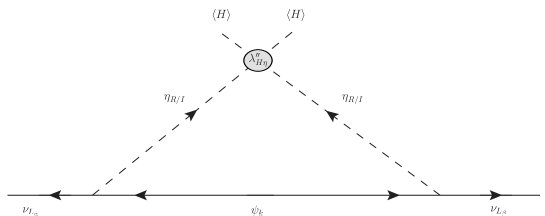
Figure 1: The one loop diagram which induces neutrino masses.

II.4 Masses for the lepton sector

The charged lepton masses are given by $m_{\ell}=y_{\ell}v/\sqrt{2}$ after the electroweak symmetry breaking, where $m_{\ell}$ is assumed to be the mass eigenstate. The neutrino mass matrix is induced at the one-loop level in Fig. 1 Ma:2006km , and its formula is given by

$$({\cal M}_{\nu})_{\alpha\beta}=\sum_{k=2}^{3}\frac{Y_{\alpha k}m_{\psi_{k}}(Y^{T})_{k\beta}}{(4\pi)^{2}}\left[\frac{m^{2}_{\eta_{R}}}{m^{2}_{\eta_{R}}-m^{2}_{\psi_{k}}}\ln\frac{m^{2}_{\eta_{R}}}{m^{2}_{\psi_{k}}}-\frac{m^{2}_{\eta_{I}}}{m^{2}_{\eta_{I}}-m^{2}_{\psi_{k}}}\ln\frac{m^{2}_{\eta_{I}}}{m^{2}_{\psi_{k}}}\right],$$ (II.33)

where we redefine $Y_{a\alpha}\equiv\sum_{i=2}^{3}\frac{y_{\nu_{ai}}V^{T}_{N_{i\alpha}}}{\sqrt{2}}$. Notice here that massless fermion $\psi_{1}$ does not contribute to the neutrino masses and their oscillations. Thus components $Y_{a1}$ do not get any constraints from neutrino mass. Once we define $D_{\nu}\equiv U_{MNS}{\cal M}_{\nu}U_{MNS}^{T}\equiv U_{MNS}(YRY^{T})U_{MNS}^{T}$, $(Y)_{3\times 2}$ can be rewritten in terms of observables and several arbitral parameters as:

$$Y_{\alpha i}=\left(U^{\dagger}_{MNS}D_{\nu}^{1/2}OR^{-1/2}\right)_{\alpha i},\quad R\equiv\frac{m_{\psi}}{(4\pi)^{2}}\left[\frac{m^{2}_{\eta_{R}}}{m^{2}_{\eta_{R}}-m^{2}_{\psi}}\ln\frac{m^{2}_{\eta_{R}}}{m^{2}_{\psi}}-\frac{m^{2}_{\eta_{I}}}{m^{2}_{\eta_{I}}-m^{2}_{\psi}}\ln\frac{m^{2}_{\eta_{I}}}{m^{2}_{\psi}}\right],$$ (II.34)

where $O\equiv O(z)$, satisfying $O^{T}O=1_{2\times 2}$ but $OO^{T}=$diag(0,1,1), is an arbitral 3 by 2 matrix with complex value of $z$, and $U_{MNS}$ and $D_{\nu}$ are obsrevables Gonzalez-Garcia:2014bfa . Depending on the mass ordering of active neutrinos, $O$ can concretely be parametrized by

$$O=\left[\begin{array}[]{cc}0&0\\ \cos z&-\sin z\\ \pm\sin z&\pm\cos z\\ \end{array}\right],\ {\rm for\ NH},\ \left[\begin{array}[]{cc}\cos z&-\sin z\\ \pm\sin z&\pm\cos z\\ 0&0\\ \end{array}\right],\ {\rm for\ IH},\$$ (II.41)

where NH(IH) is short-hand notation of ”Normal(Inverted) Hierarchy”, and the lightest active neutrino mass is zero.

II.5 Lepton flavor violations

LFV processes $\ell\to\ell^{\prime}\gamma$ are induced from the neutrino Yukawa couplings at one-loop level, and their forms are given by

$$BR(\ell_{\alpha}\to\ell_{\beta}\gamma) \approx\frac{4\pi^{3}\alpha_{em}C_{\alpha\beta}}{3(4\pi)^{4}G_{F}^{2}}\left|\sum_{i=2}^{3}(Y)_{\beta i}(Y^{\dagger})_{i\alpha}F_{lfv}(\psi_{i},\eta^{\pm})\right|^{2},$$ (II.42)

$$F_{lfv}(a,b) \equiv\frac{2m_{a}^{6}+3m_{a}^{4}m_{b}^{2}-6m_{a}^{2}m_{b}^{4}+m_{b}^{6}+12m_{a}^{4}m_{b}^{2}\ln\left[\frac{m_{b}}{m_{a}}\right]}{(m_{a}^{2}-m_{b}^{2})^{4}},$$ (II.43)

where $\alpha_{em}\approx 1/134$ is the fine-structure constant, $G_{F}\approx 1.17\times 10^{-5}$ GeV^-2 is the Fermi constant, and $C_{21}\approx 1$, $C_{31}\approx 0.1784$, $C_{32}\approx 0.1736$. The stringent constraint comes from $\mu\to e\gamma$ and its upper bound is given by $BR(\mu\to e\gamma)\lesssim 4.2\times 10^{-13}$ TheMEG:2016wtm .

II.6 Dark matter

Here we discuss if our model can have viable DM candidate. In general, this class of model has two kinds of DM candidates; the lightest fermion $m_{\psi_{1}}$ and/or the lightest neutral inert boson $m_{\eta_{R}}$. However since the lightest fermion is massless, an inert boson is in favor of being the good DM candidate. Even when it is the case, one might worry about the too fast decay of DM; the decay mode $\eta_{R}\to\nu_{L}\psi_{1}$ arises from $y_{\nu}$, and its decay rate is written by $\Gamma\sim\frac{m_{\eta_{R}}}{16\pi^{2}}\sum_{a=1}^{3}|(Y)_{a1}|^{2}$. Then we evaluate the upper bound on $\Gamma$ by imposing its lifetime $\tau$ ($\Gamma=\tau^{-1}$) should be longer than the current Universe, therefore we have the following constraint:

$$\Gamma\lesssim 1.51\times 10^{-42}\ {\rm GeV}.$$ (II.44)

Although we can take $\sum_{a=1}^{3}|(Y)_{a1}|^{2}$ as free parameters because it does not contribute to the neutrino oscillation data, the above constraint severely restricts our model. In addition, we need to take into account quantum corrections to the couplings to check the constraint can be satisfied at low scale. In principle, our requirement can be realized by tuning the free parameters. Therefore one can have viable DM candidate if we imposing fine tuning for the Yukawa couplings.

If one assumes that there exists DM in our theory, which is inert boson $\eta_{R}$, one has to rely on modes via kinetic term and/or Higgs potential to explain the relic density of DM; $\Omega h^{2}\approx$0.12 Ade:2013zuv . When the mode from Higgs portal interaction is subdominant due to constraint from DM direct detection searches, the main mode comes from gauge interactions in kinetic term. Note that we have $Z^{\prime}$ interaction of inert boson $\eta_{R}$ as it is charged under the extra $U(1)$. However the $Z^{\prime}$ interaction will be subdominant since we should require heavy $Z^{\prime}$ mass as $\gtrsim$ few TeV or small gauge coupling $g_{BL}$ due to current LHC constraints. In addition, the $Z^{\prime}$ interaction takes the form of $Z^{\prime}_{\mu}(\partial^{\mu}\eta_{R}\eta_{I}-\eta_{R}\partial^{\mu}\eta_{I})$ and it does not contribute to DM-nucleon scattering if masses of $\eta_{R}$ and $\eta_{I}$ are not much degenerated ; $Z^{\prime}$ exchange contributes to DM-nucleon scattering if $\eta_{R}$ and $\eta_{I}$ have degenerate masses  . Hence the DM feature is almost the same as two Higgs doublet model with an inert Higgs, which has already been discussed in ref. Hambye:2009pw . Therefore the allowed mass is at around $\gtrsim 500$ GeV, once the W/Z final state modes are opened.

II.7 The effective number of neutrino species: $\Delta N_{\rm eff}$

The massless fields contribute to the relativistic energy density of Universe, which is denoted by $\Delta N_{\rm eff}$. A thermalized scalar(fermion) contributes $\Delta N_{\rm eff}=4/7(1)$, each of which is consistent with bounds from Big Bang Nucleosynthesis (BBN), which are in the range of $\Delta N_{\rm eff}<1.2$ Mangano:2011ar at 95% CL, depending on the primordial abundances. Moreover, once we assume that these fields typically decouple from the plasma at temperatures above the QCD phase transition $\sim\cal O$(100) MeV, we find the effective number of relativistic degrees of freedom to be about 60. Therefore we obtain

$$\Delta N_{\rm eff}\lesssim\frac{11}{7}\left(\frac{10.75}{60}\right)^{4/3}\approx 0.159.$$ (II.45)

This value is still in good agreement with the recent experimental data such as Planck $\Delta N_{\rm eff}=0.15\pm 0.23$ Ade:2015xua . Note that although massless particles are charged under $B-L$ they interact with the SM particles by exchanging heavy $Z^{\prime}$ and/or scalar bosons which are $\mathcal{O}(100)$ GeV or $\mathcal{O}(1)$ TeV scale. Thus our massless particles can be decoupled at the early Universe before QCD phase transition. Here BBN occurs after QCD phase transition.

II.8 Numerical analysis

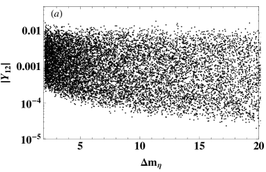
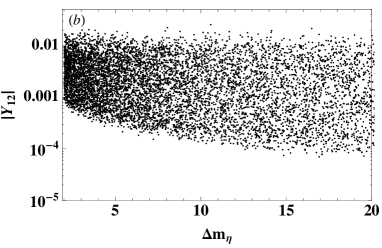
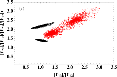
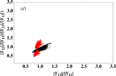
Figure 2: (a) and (b): Correlation between $Y_{12}$ and $\Delta m_{\eta}$ for NH (a) and IH (b) cases. (c) and (d): correlation between $|Y_{13}|/|Y_{12}|$ and $|Y_{22(23)}|/|Y_{12}|$ by balck(red) dots for NH (c) and IH (d) cases. (e) and (f): correlation between $|Y_{32}|/|Y_{12}|$ and $|Y_{33}|/|Y_{12}|$ for NH (e) and IH (f) cases.

Here we explore the allowed region to satisfy neutrino oscillation data and constraint from BR$(\ell\to\ell^{\prime}\gamma)$. First of all, we randomly select the following input parameters:

$${\rm Re}[z]\in(0,\pi),\quad{\rm Im}[z]\in(1,10),$$

$$(M_{NS_{1,2}},M_{S})\in(1,500)\ {\rm GeV},\quad m_{\eta_{R}}\in(100,500)\ {\rm GeV},$$

$$\Delta m_{\eta}\in(2,20)\ {\rm GeV},\quad m_{\eta^{\pm}}=m_{\eta_{I}}=\sqrt{m_{\eta_{R}}^{2}+\Delta m_{\eta}^{2}},$$ (II.46)

where we take the typical region of the parameters as discussed above. Here we also apply a condition $m_{\eta_{R}}<m_{\psi_{2,3}}$ expecting $\eta_{R}$ to be a DM candidate. In addition we apply best fit values of the current neutrino oscillation data for NH and IH cases Olive:2016xmw . As our outputs we obtain $Y_{\alpha i}$ ($\alpha=1-3$, $i=1,2$) from our formula Eq. (II.34). Firstly, we show correlation between the size of Yukawa coupling $|Y_{12}|$ and $\Delta m_{\eta}$ in Fig. 2-(a) and -(b) for NH and IH cases. Moreover relative size of the Yukawa couplings $|Y_{\alpha i}|/|Y_{12}|$ are shown in Fig. 2-(c,e) and -(d,f) for NH and IH cases. From the figures we see the typical size of $|Y_{\alpha i}|$ is $\mathcal{O}(10^{-4})$ to $\mathcal{O}(10^{-2})$. Thus original couplings in the Lagrangian $y_{\nu}$ have the same order of values and it is similar to the size of $y_{\ell}$ which provide charged lepton masses. Also we find that the correlations among the Yukawa couplings are clearly different between NH and IH cases. Fig. 3 shows the scattering plots to satisfy the neutrino oscillation data and LFVs in terms of the correlation between $m_{\psi_{1}}$ and $m_{\psi_{2}}$, where the the left(right) figure represents the case of NH(IH). The Fig. 4 shows the scattering plots in terms of the correlation between the values of LFVs and $m_{\psi_{2}}$, where the left(right) figure represents the case of NH(IH). The points of red, green, and blue respectively represent the case of $BR(\mu\to e\gamma)$, $BR(\tau\to e\gamma)$, and $BR(\tau\to\mu\gamma)$. The Fig. 5 shows the scattering plots to satisfy the neutrino oscillation data and LFVs in terms of the correlation between $m_{\eta_{R}}$ and $m_{\psi_{2/3}}$, where the left(right) figure represents the case of NH(IH). The points of black and red respectively represent the case of $m_{\psi_{2}}$ and $m_{\psi_{3}}$. These figures suggest that there are no difference between NH and IH for the masses of $m_{\psi_{2,3,\eta_{R}}}$, while the LFVs give differences among each processes; upper bound on $\tau\to e\gamma$ in the NH case is lower than the other two processes, while upper bound on $\mu\to e\gamma$ in the IH case is higher than the other two processes by half. And orders of upper bounds for three processes for NH and IH are respectively found to be $10^{-13}$ and $10^{-14}$.

Figure 3: Scattering plots to satisfy the neutrino oscillation data and LFVs in terms of the correlation between $m_{\psi_{1}}$ and $m_{\psi_{2}}$, where the the left(right) figure represents the case of NH(IH).

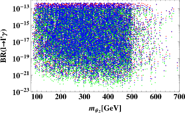
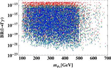
Figure 4: Scattering plots in terms of the correlation between the values of LFVs and $m_{\psi_{2}}$, where the the left(right) figure represents the case of NH(IH). The points of red, green, and blue respectively represent the case of $BR(\mu\to e\gamma)$, $BR(\tau\to e\gamma)$, and $BR(\tau\to\mu\gamma)$.

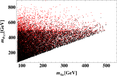
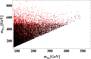
Figure 5: Scattering plots to satisfy the neutrino oscillation data and LFVs in terms of the correlation between $m_{\eta_{R}}$ and $m_{\psi_{2/3}}$, where the the left(right) figure represents the case of NH(IH). The points of black and red respectively represent the case of $m_{\psi_{2}}$ and $m_{\psi_{3}}$.

III Conclusion

We have proposed a model based on an alternative $U(1)_{B-L}$ gauge symmetry with 5 dimensional operators in the Lagrangian in which we have constructed the neutrino masses at one-loop level introducing minimal field contents, and discussed LFVs, DM, and $\Delta N_{\rm eff}$. Then numerical analysis is carried out to search for values of parameters accommodating observed data adopting some input parameter without tuning. As a result we have found allowed region to satisfy all the data such as neutrino oscillation data without conflict of several constraints such as LFV and $\Delta N_{\rm eff}$. Below we list several remarks:

1. To estimate our cut-off scale, we have assumed that the initial value of gauge coupling $g_{BL}$ at $m_{Z}$ is same as the one of hypercharge $g_{Y}$; $g_{BL}(m_{Z})=g_{Y}(m_{Z})$. Then we have obtained $\Lambda=100$ TeV, then the mass difference between $\eta_{R}$ and $\eta_{I}$ is of the order 0.1 GeV under $v=246$ GeV, $v_{\varphi_{6}}=1$ TeV, and $\lambda^{\prime\prime}_{H\eta}=1$. Since it contributes to the neutrino masses, more natural parametrization has been achieved to explain the scale of neutrino masses. Of course, we can always increase the value of $\Lambda$, by enlarging the initial value of $g_{BL}$.

2. Lightest active neutrino is massless that arises from rank two matrix of $\psi$. Through our numerical analyses, there are no difference between NH and IH for the masses of $m_{\psi_{2,3,\eta_{R}}}$ while we have found correlations among relative sizes of the Yukawa couplings related to $\bar{L}_{L}\tilde{\eta}N_{R}$ terms. Also typical order of the Yukawa couplings is $\mathcal{O}(10^{-4})$ to $\mathcal{O}(10^{-2})$ which is similar to SM Yukawa couplings for charged lepton masses. In addition the LFVs give differences among each processes; upper bound on $\tau\to e\gamma$ in the NH case is lower than the other two processes, while upper bound on $\mu\to e\gamma$ in the IH case is higher than the the other two processes by half. And orders of upper bounds for three processes for NH and IH are respectively found to be $10^{-13}$ and $10^{-14}$.

3. DM candidate in the model is neutral component of inert scalar doublet since the lightest component of $\psi$ is massless. However inert boson can decay into $\psi_{1}\nu_{L}$ via Yukawa interaction. We find that one can in principle stabilize the DM candidate by fine-tuning the parameters since the Yukawa interactions related to DM are free parameters due to absence of neutrinos masses. In addition relic density of DM can be realized as in the inert Higgs doublet model. Thus it is possible to accommodate DM in our model if we require fine-tuning for the Yukawa couplings.

4. We have simply estimated $\Delta N_{\rm eff}$, since we have a physical massless fermion in addition to the massless boson. And we have confirmed it is still within experiment by Planck.

Note that relative size of Yukawa couplings $Y_{\alpha i}$ is related to decay branching ratio of $\eta^{\pm}$ which decays into $\ell^{\pm}\Psi_{i}$ via Yukawa interactions. Thus prediction to the correlation among the Yukawa couplings would be tested by searching for signals from $\eta^{\pm}$ production at collider like LHC.

Appendix A Beta function of $g_{BL}$

Here we discuss running of $g_{BL}$ coupling and estimate the effective energy scale by evaluating the Landau pole due the presence of new fields. Each of $B-L$ beta function for boson and fermion is given by

$$b^{b}_{B-L}=33,\quad b^{f}_{B-L}=\frac{140}{3}.$$ (A.1)

Then one finds the following energy evolution of the gauge coupling:

$$\frac{1}{g^{2}_{B-L}(\Lambda)} =\frac{1}{g_{B-L}^{2}(m_{in.})}-\theta(\Lambda-m_{th.})\frac{b^{b}_{B-L}+b^{f}_{B-L}}{(4\pi)^{2}}\ln\left[\frac{\Lambda^{2}}{m_{th.}^{2}}\right],$$ (A.2)

where $\Lambda$ is a reference energy, and we assume to be $m_{in.}(=m_{Z})<m_{th.}=$100 GeV, with the same threshold masses $m_{th.}$ for fermions and bosons. Once we fix to be $g_{BL}(m_{in.})=g_{Y}(m_{in.})$, we obtain the RGE flow as can be seen in Fig. 6. It shows that $g_{BL}$ is valid up to around 100 TeV. Notice here that RGE is very sensitive to the initial value of $g_{BL}$, and we can always enlarge the cut-off scale by decreasing the value of $g_{BL}$. For example if one fix to be $g_{BL}(m_{in.})=0.1\times g_{Y}(m_{in.})$, then the theory is valid up to Plank mass scale $\sim 10^{18}$ GeV.

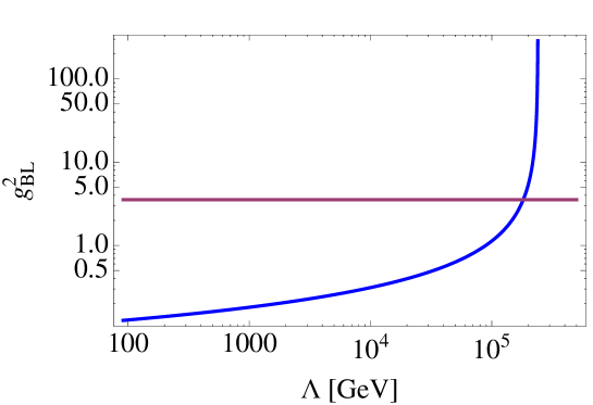
Figure 6: RGE flow of $g_{BL}$ in terms of cut-off scale $\Lambda$, where $g_{Y}(m_{in.})=g_{BL}(m_{in.})$ is assumed.

References

- (1) K. S. Babu and R. N. Mohapatra, Phys. Rev. Lett. 70, 2845 (1993) [hep-ph/9209215].
- (2) R. N. Mohapatra and J. W. F. Valle, Phys. Rev. D 34 (1986) 1642.
- (3) J. C. Montero and V. Pleitez, Phys. Lett. B 675, 64 (2009).
- (4) E. Ma and R. Srivastava, Phys. Lett. B 741, 217 (2015) doi:10.1016/j.physletb.2014.12.049 [arXiv:1411.5042 [hep-ph]].
- (5) E. Ma and R. Srivastava, Mod. Phys. Lett. A 30, no. 26, 1530020 (2015) doi:10.1142/S0217732315300207 [arXiv:1504.00111 [hep-ph]].
- (6) S. Patra, W. Rodejohann and C. E. Yaguna, JHEP 1609, 076 (2016).
- (7) S. Singirala, R. Mohanta and S. Patra, arXiv:1704.01107 [hep-ph].
- (8) T. Nomura and H. Okada, arXiv:1705.08309 [hep-ph].
- (9) T. Nomura and H. Okada, arXiv:1708.08737 [hep-ph].
- (10) T. Nomura and H. Okada, arXiv:1709.06406 [hep-ph].
- (11) D. Nanda and D. Borah, arXiv:1709.08417 [hep-ph].
- (12) S. Singirala, R. Mohanta, S. Patra and S. Rao, arXiv:1710.05775 [hep-ph].
- (13) C. Q. Geng and H. Okada, Phys. Dark Univ. 20, 13 (2018) doi:10.1016/j.dark.2018.02.005 [arXiv:1710.09536 [hep-ph]].
- (14) E. Ma, Phys. Rev. D 73, 077301 (2006) [hep-ph/0601225].
- (15) M. Aoki, J. Kubo and H. Takano, Phys. Rev. D 87, no. 11, 116001 (2013) doi:10.1103/PhysRevD.87.116001 [arXiv:1302.3936 [hep-ph]].
- (16) H. Okada and T. Toma, Phys. Rev. D 86, 033011 (2012) [arXiv:1207.0864 [hep-ph]].
- (17) Y. Kajiyama, H. Okada and T. Toma, Eur. Phys. J. C 73, no. 3, 2381 (2013) [arXiv:1210.2305 [hep-ph]].
- (18) S. Choi, S. Jung and P. Ko, JHEP 1310, 225 (2013) [arXiv:1307.3948 [hep-ph]].
- (19) K. Cheung, P. Ko, J. S. Lee and P. Y. Tseng, JHEP 1510, 057 (2015) [arXiv:1507.06158 [hep-ph]].
- (20) G. Belanger, K. Kannike, A. Pukhov and M. Raidal, JCAP 1204, 010 (2012) [arXiv:1202.2962 [hep-ph]].
- (21) M. Aoki, D. Kaneko and J. Kubo, arXiv:1711.03765 [hep-ph].
- (22) M. Aaboud et al. [ATLAS Collaboration], arXiv:1707.02424 [hep-ex].
- (23) M. Klasen, F. Lyonnet and F. S. Queiroz, Eur. Phys. J. C 77, no. 5, 348 (2017) [arXiv:1607.06468 [hep-ph]].
- (24) H. Fukuoka, J. Kubo and D. Suematsu, Phys. Lett. B 678, 401 (2009) [arXiv:0905.2847 [hep-ph]].
- (25) M. C. Gonzalez-Garcia, M. Maltoni and T. Schwetz, JHEP 1411, 052 (2014) [arXiv:1409.5439 [hep-ph]].
- (26) K. Hayasaka et al. [Belle Collaboration], Phys. Lett. B 666, 16 (2008) [arXiv:0705.0650 [hep-ex]].
- (27) G. Mangano and P. D. Serpico, Phys. Lett. B 701, 296 (2011) [arXiv:1103.1261 [astro-ph.CO]].
- (28) P. A. R. Ade et al. [Planck Collaboration], Astron. Astrophys. 594, A13 (2016) [arXiv:1502.01589 [astro-ph.CO]].
- (29) D. S. Akerib et al. [LUX Collaboration], Phys. Rev. Lett. 118, no. 2, 021303 (2017) [arXiv:1608.07648 [astro-ph.CO]].
- (30) A. M. Baldini et al. [MEG Collaboration], Eur. Phys. J. C 76, no. 8, 434 (2016).
- (31) P. A. R. Ade et al. [Planck Collaboration], Astron. Astrophys. 571, A16 (2014) [arXiv:1303.5076 [astro-ph.CO]].
- (32) T. Hambye, F.-S. Ling, L. Lopez Honorez and J. Rocher, JHEP 0907, 090 (2009) Erratum: [JHEP 1005, 066 (2010)] [arXiv:0903.4010 [hep-ph]].
- (33) E. Ma, N. Pollard, R. Srivastava and M. Zakeri, Phys. Lett. B 750, 135 (2015) doi:10.1016/j.physletb.2015.09.010 [arXiv:1507.03943 [hep-ph]].
- (34) K. Nishiwaki, H. Okada and Y. Orikasa, Phys. Rev. D 92, no. 9, 093013 (2015) [arXiv:1507.02412 [hep-ph]].
- (35) S. Schael et al. [ALEPH and DELPHI and L3 and OPAL and LEP Electroweak Collaborations], Phys. Rept. 532, 119 (2013) [arXiv:1302.3415 [hep-ex]].
- (36) R. Barbieri, L. J. Hall and V. S. Rychkov, Phys. Rev. D 74, 015007 (2006) [hep-ph/0603188].
- (37) C. Patrignani et al. [Particle Data Group], Chin. Phys. C 40, no. 10, 100001 (2016).