Impact of climate change on backup energy and storage needs in wind-dominated power systems in Europe

Abstract

The high temporal variability of wind power generation represents a major challenge for the realization of a sustainable energy supply. Large backup and storage facilities are necessary to secure the supply in periods of low renewable generation, especially in countries with a high share of renewables. We show that strong climate change is likely to impede the system integration of intermittent wind energy. To this end, we analyze the temporal characteristics of wind power generation based on high-resolution climate projections for Europe and uncover a robust increase of backup energy and storage needs in most of Central, Northern and North-Western Europe. This effect can be traced back to an increase of the likelihood for long periods of low wind generation and an increase in the seasonal wind variability.

Introduction

The mitigation of climate change requires a fundamental transformation of our energy system. Currently, the generation of electric power with fossil fuel-fired power plants is the largest source of carbon dioxide emissions with a share of approximately 35 % of the global emissions Bruc14 . These power plants must be replaced by renewable sources such as wind turbines and solar photovoltaics (PV) within at most two decades to meet the 2^∘C or even the 1.5^∘C goal of the Paris agreement Paris15 ; roge15 ; Rogelj16 . While wind and solar power have shown an enormous progress in efficiency and costs Jacobson11 ; Sims11 , the large-scale integration into the electric power system remains a great challenge.

The operation of wind turbines is determined by weather and climate and thus strongly depends on the regional atmospheric conditions. Hence, the generated electric power is strongly fluctuating on different time scales. These fluctuations are crucial for system operation Bloo16 ; olau16 ; davi16 ; Sims11 ; Hube14 ; weber17 . In particular, large storage and backup facilities are needed to guarantee supply also during periods of low wind generation Heid10 ; Elsn15 ; diaz12 . How does climate change affect these fluctuations and the challenges of system integration? Previous studies have addressed the impact of climate change on the availability of cooling water Vlie12 ; Vlie16 , the energy demand Allen2016 ; Auffhammer2017 , or the change of global energy yields of wind and solar power pryo10 ; Tobi15 ; Tobi16 ; Reye15 ; Reye16 ; 2017Moemken ; Jere15 ; stan16 . However, the potentially crucial impact of climate change on temporal wind fluctuations has not yet been considered in terms of system integration.

A consensus exists about general changes in the mean sea level pressure and circulation patterns in the European/North Atlantic region Demu09 ; Woll12 ; Zapp15 ; Lu07 . A projected increase of the winter storminess over Western Europe Pint12 ; Fese15 leads to enhanced wind speeds over Western and Central Europe, while in summer a general decrease is identified hueg13 ; Reye15 ; Reye16 ; 2017Moemken . This can lead to a strong increase of the seasonal variability of wind power generation and thus impede system integration, even though the annual mean changes are comparatively small.

In this article, we study how climate change affects the temporal characteristics of wind power generation and the necessity for backup and storage infrastructures in wind-dominated power systems in individual European countries. Our analysis is based on five state-of-the-art global circulation models (GCMs) downscaled by the EURO-CORDEX initiative Jaco14 ; gior15 . We complement our results with an assessment of the large ensemble of the Coupled Model Intercomparison Project Phase 5 (CMIP5, Tayl12 ) based on circulation weather types Jone93 . The paper is organized as follows. We first introduce our model to derive the backup need of a country as a function of the storage capacity. Additionally, we present the methods to analyze the CMIP5 ensemble. Afterwards we report our results. The article closes with a discussion.

Methods

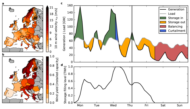
Figure 1: Conversion of near-surface wind speeds to country-wise aggregated wind power generation combined with backup and storage infrastructures. a, Near-surface wind velocities of the downscaled ERA-Interim data dee11 over Europe for one exemplary point in time. b, Corresponding estimated wind power yield for each country in units of the installed capacity. c, Renewable generation (black) and load (grey) in Germany for one exemplary week in spring assuming a power system with 100 % wind power on average. The vertical line denotes the time selected in panels a and b. The color indicates the operation of the storage system. Green: Excess power is stored. Yellow: Residual load is covered by the storage. Red: Residual load is covered by backup power plants as the storage is empty. Blue: Excess power must be curtailed as the storage is fully charged. d, Evolution of the storage filling level $S(t)$.

The operation of future renewable power systems with large contributions of wind crucially depends on weather and climate. GCMs are used to simulate the dynamics of the earth system on coarse spatial scales for different scenarios of future greenhouse gas concentrations (representative concentration pathways, RCPs Vuur11 ). To analyze the operation of the electric power system, a high spatial and temporal resolution is required. Our analysis is thus based on a subset of the EURO-CORDEX ensemble which provides dynamically downscaled climate change data at high resolution ($0.11^{\circ}$ and 3 hours). Time series for the aggregated wind power generation in a country are obtained from the near-surface wind speed (see Fig. 1a, b).

Backup and storage infrastructures are needed when renewable generation drops below load. In order to quantify the necessary amount of backup and storage to ensure a stable supply, we adopt a coarse-grained model of the electric power system (see Fig. 1c, d). Backup and storage needs crucially depend on the temporal characteristics of wind power generation, in particular the length of periods with low wind generation and the seasonal variability. In the present paper, we thus focus on temporal characteristics and their potential alteration due to climate change.

Wind power generation time series

Our analysis is based on a subset of the EURO-CORDEX regional climate simulations which provides dynamically downscaled climate change data at high resolution for Europe based on five GCMs: CNRM-CM5, EC-EARTH, HadGEM2-ES, IPSL-CM5A-MR, MPI-ESM-LR Jaco14 (see also Table S1 in Appendix A). All data is freely available for example at the ESGF (Earth System Grid Federation) node at DKRZ (German Climate Computing Centre) esgf . The five models are downscaled using the hydrostatic Rossby Centre regional climate model RCA4 Stra15 ; Samu11 . The downscaling provides continuous surface (10 m) wind data from 1970 to 2100 with a spatial resolution of $0.11^{\circ}$ and a temporal resolution of $T=$ 3 hours. Unfortunately, downscaled data at this high spatial and temporal resolution is not yet available for more GCMs or for different regional climate models at ESGF esgf . Considering the use of only one regional climate model, 2017Moemken show that differences between different GCMs are usually larger than differences between different regional climate models.

We analyze a strong climate change scenario (RCP8.5) using a rising radiative forcing pathway leading to additional 8.5 W/m² ($\sim$1370 ppm CO₂ equivalent) by 2100 and a medium climate change scenario (RCP4.5, $\sim$650 ppm CO₂ equivalent, see Appendix C) Vuur11 . We compare two future time frames, 2030-2060 (mid century, ‘mc’) and 2070-2100 (end of century, ‘eoc’), to a historical reference time frame (1970-2000, ‘h’).

The calculation of wind power generation requires wind speeds at the hub height of wind turbines. As the high resolution wind velocities are only available at a height of $z_{0}=10$ m, they must be extrapolated to a higher altitude. We choose a hub height of $z=90$ m as in Tobi16 and extrapolate the surface wind velocities $v_{z_{0}}$ using a power law formula: $v_{z}=v_{z_{0}}\left({z}/{z_{0}}\right)^{1/7}$ Manwell09 . Although widely used, this simple formula is only valid for smooth open terrain and only applies for a neutrally stable atmosphere. Unfortunately, the available data set does not allow to assess the stability of the atmosphere. Thus, it is unclear how to improve the scaling law with the present data available. Tobin et al. Tobi16 show in a sensitivity study that their results hardly depend on the extrapolation technique or on the chosen hub height. They further state that the “uncertainty related to climate model formulation prevails largely over uncertainties lying in the methodology used to convert surface wind speed into power output”.

The wind generation is derived using a standardized power curve with a cut-in wind speed of $v_{i}=3.5$ m/s, a rated wind speed of $v_{r}=12$ m/s and a cut-out wind speed of $v_{o}=25$ m/s as in Tobi16 . The capacity factor $CF(t)$ (i.e. the generation normalized to the rated capacity) then reads

$$CF(t)=\left\{\begin{array}[]{@{\kern 2.5pt}lL}\hfill 0&if $v_{z}(t)<v_{i}$ or $v_{z}(t)\geq v_{o}$.\\ \hfill\frac{v_{z}^{3}(t)-v_{i}^{3}}{v_{r}^{3}-v_{i}^{3}}&if $v_{i}\leq v_{z}(t)$,\\ \hfill 1&else.\end{array}\right.$$ (1)

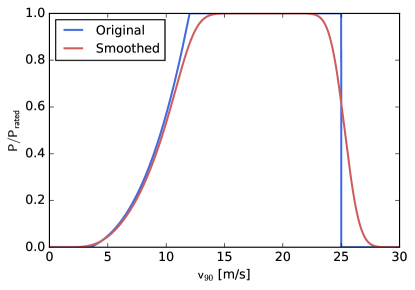
Figure S1: Power curve. Power curve used to convert wind velocities in a height of 90 m ($v_{90}$) to wind power generation data. In order to account for wind farms and velocity variations the single turbine power curve (blue) is smoothed using a gaussian kernel (red).

In order to account for wind farms and velocity variations, the power curve is smoothed using a gaussian kernel (see Fig. S1 in Appendix A and Andresen15 ; Manwell09 ).

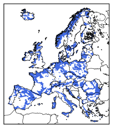
Figure S2: Placement of wind farms. Wind farms are homogeneously placed on colored sites. On these sites the 31-year average of the wind yield is higher than the country average. For this derivation, ERA-Interim data dee11 is used. In a sensitivity study, wind farms are placed homogeneously at each grid point inside a country (see Figs S13, S14 and S15 in Appendix D).

To obtain the gross generation per country, we equally distribute wind farms on grid points for which the local average wind yield is higher than the country average (see Fig. S2 in Appendix A) Monf16 . Offshore sites are not considered as we want to focus on effects of climate change on onshore wind power generation in this study. The distribution is fixed using historical reanalysis data from ERA-Interim dee11 downscaled by the EURO-CORDEX initiative Jaco14 ; Stra15 to guarantee consistency (cf. Fig. 1b). We do not use the wind farm distribution as of today because installed capacities in a fully-renewable power system will be much higher and also more widespread than they are today such that wind parks will be built in yet unused locations. Furthermore, Monf16 show that different wind farm distributions do not significantly affect the results (see also Figs S13, S14 and S15 in Appendix D where we tested a homogeneous wind farm distribution within each country).

Wind power generation is aggregated using two approaches: (a) aggregation per country neglecting transmission constraints, assuming an unlimited grid within each country; (b) aggregation over the whole European continent, assuming a perfectly interconnected European power system (copperplate). The intermediate case is discussed for instance in Rodriguez2014 ; Schlachtb16 for current climatic conditions and in 2017Wohland for a changing climate but without considering storage.

For the load time series $L(t)$ we use data of the year 2015 provided by the European Network of Transmission System Operators for Electricity (ENTSO-E, entsoe_load ) and repeat this year 31 times. In order to avoid trends in the load timeseries, we consider a single year only. Furthermore, we show in a sensitivity study assuming constant loads that our results dominantly depend on the generation timeseries and are hardly affected by the load time series (see Fig. S12 in Appendix D). Throughout all time frames we assume that wind power provides a fixed share $\gamma$ of the load $L(t)$ per country Heid10 . Hence, the fluctuating wind power generation $R(t)$ is scaled such that

$$R(t)=\gamma\,\frac{CF(t)}{\langle CF(t)\rangle}\,\langle L(t)\rangle,$$ (2)

where the brackets denote the average over the respective time frame for a given model. This procedure normalizes out a possible change of the gross wind power yield, and thus allows to isolate the effects of a change in the temporal distribution of the renewable generation. For the copperplate assumption, the wind power generation is scaled such that each country provides a fixed share $\gamma$ of the country-specific load. Afterwards, the country-specific wind power generation is summed-up to one aggregated time series. In the main manuscript, we focus on a fully renewable power system per country, i.e., $\gamma=1$, with 100 % wind power generation. Results for different values of $\gamma$ are shown in Figs S10 and S11 in Appendix D.

Calculation of backup energy needs

Country-wise aggregated wind generation and load data are used to derive the backup energy need of a country given different storage capacities. At each point of time $t$ power generation and consumption of a country must be balanced Heid10 ; Rasm12 ; Rodriguez2014

$$R(t)+B(t)=\Delta(t)+L(t)+C(t),$$ (3)

where $R(t)$ and $B(t)$ denote the generation by fluctuating renewables and dispatchable backup generators, respectively, $L(t)$ is the load and $C(t)$ denotes curtailment (cf. Fig. 1c). $\Delta(t)$ is the generation ($\Delta(t)<0$) or load ($\Delta(t)>0$) of the storage facilities, such that the storage filling level evolves according to (cf. Fig. 1d)

$$S(t+T)=S(t)+\Delta(t)\cdot T.$$ (4)

where $T$ is the duration of one time step (here: 3 hours). The storage filling level must satisfy $0\leq S(t)\leq S_{\rm max}$ with $S_{\rm max}$ being the storage capacity. We decide to minimize the total backup energy $B_{\rm tot}=\sum_{t}B(t)\cdot T$ which also minimizes fossil-fuel usage and hence greenhouse gas emissions. This yields a storage-first strategy Rasm12 : In the case of overproduction (i.e. $R(t)>L(t)$) excess energy is stored until the storage device is fully charged,

$$\Delta(t)=\min[R(t)-L(t);(S_{\rm max}-S(t))/T].$$ (5)

To ensure power balance, we may need curtailment

$$C(t)=R(t)-L(t)-\Delta(t).$$ (6)

In the case of scarcity (i.e. $R(t)<L(t)$) energy is provided by the storage infrastructures until they are empty,

$$\Delta(t)=-\min[L(t)-R(t);S(t)/T].$$ (7)

The missing energy has to be provided by backup power plants,

$$B(t)=L(t)-R(t)+\Delta(t).$$ (8)

The backup power $B$ is not restricted in our model and can be interpreted as the aggregated amount of backup power per country, not differentiating between different technologies. In order to keep the storage neutral, a periodic boundary condition ($S(t=t_{\rm max})=S(t=0)$) is applied Jens14 . We emphasize that by the term ‘storage’ we mean storage regardless of the technical realization. Hence, $S_{\rm max}$ describes the total accumulated storage capacity, including virtual storage. For simplicity, we neglect losses in the storage process.

In the figures we show the average backup energy per year $E=\langle B\rangle/\langle L\rangle\cdot L_{\rm year}$. $L_{\rm year}$ is the average yearly gross electricity demand of the respective country. Thus, $E/L_{\rm year}$ gives the share of energy that has to be provided by dispatchable backup generators Rasm12 .

Persistence of low wind situations

We measure the probability for long low wind periods during which a high amount of energy is required from storage devices and backup power plants. Therefore, we identify all periods for which the wind power generation is continuously smaller than average (i.e. $R(t)<\langle R\rangle$) and record their duration $\tau$. From this, we can estimate a probability distribution. Extreme events are quantified by the 95 % quantile of the distribution.

Seasonal wind variability

The wind yield in Europe is usually higher in winter than in summer. An increasing seasonal wind variability would refer to higher wind yields in the winter months and/or lower wind yields in the summer months and would lead to higher backup energy needs during summer.

We define the winter-summer ratio of the country-wise aggregated wind power generation as the ratio of the average winter wind generation $\langle R\rangle_{\rm DJF}$ and the average summer wind generation $\langle R\rangle_{\rm JJA}$:

$$R_{\rm winter-summer}=\frac{\langle R\rangle_{\rm DJF}}{\langle R\rangle_{\rm JJA}},$$ (9)

with ‘DJF’: December, January, February, and ‘JJA’: June, July, August. $\langle R\rangle_{\rm DJF}$ and $\langle R\rangle_{\rm JJA}$ are the mean generations within a certain time frame (historical, mid century, end of century).

Analysis of low wind periods using a statistical analysis of a large CMIP5 ensemble

Our analysis is complemented with lower resolution data of 22 GCMs contributing to the Coupled Model Intercomparison Project Phase 5 (CMIP5, Tayl12 ). The GCM output is analyzed with a statistical method developed in Reye15 ; Reye16 . We characterize the large-scale circulation over Central Europe by determining the prevalent circulation weather type (CWT, Jone93 ) using instantaneous daily mean sea level pressure (MSLP) fields around a central point at 10^∘E and 50^∘N (near Frankfurt, Germany) at 00 UTC (see also Fig 2 in Reye15 ). The different CWT classes are either directional (‘North’, ‘North-East’, ‘East’, ‘South-East’, ‘South’, ‘South-West’, ‘West’, ‘North-West’) or rotating (‘Cyclonic’, ‘Anti-cyclonic’). Additionally, a proxy for the large-scale geostrophic wind (denoted as $f$-parameter) is derived using the gradient of the instantaneous MSLP field. Higher geostrophic wind values (i.e. higher $f$-parameters) correspond to larger wind power yields in Central Europe.

In order to compare the CMIP5 and the EURO-CORDEX data, we test whether the $f$-parameter derived using the coarse ERA-Interim reanalysis data Reye15 is capable to reproduce the characteristics of German low-wind generation periods as determined from the downscaled ERA-Interim dataset dee11 . We classify days with below-average wind power generation (scarcity) for each CWT by a low value of the $f$-parameter, $f(t)\leq f_{\rm th}$, as shown in Fig. 7a. Thus, for each day, we can analyze whether the classifier ($f(t)\leq f_{\rm th}$) correctly predicts that the wind power generation is below average ($R(t)<\langle R\rangle$) or erroneously predicts that the wind power generation is above average ($R(t)\geq\langle R\rangle$). The quality of this classification is quantified by the fraction of true predictions, called sensitivity

$${\rm SEN}=\frac{n[{R<\langle R\rangle\,\&\,f\leq f_{\rm th}}]}{n[{R<\langle R\rangle\,\&\,f\leq f_{\rm th}}]+n[{R<\langle R\rangle\,\&\,f>f_{\rm th}}]}$$ (10)

and the fraction of false predictions

$${\rm FFP}=\frac{n[{R\geq\langle R\rangle\,\&\,f\leq f_{\rm th}}]}{n[{R\geq\langle R\rangle\,\&\,f\leq f_{\rm th}}]+n[{R\geq\langle R\rangle\,\&\,f>f_{\rm th}}]},$$ (11)

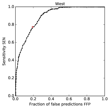
Figure S3: ROC curve. Receiver operating characteristic (ROC) curve to assess the performance of the $f$-parameter to classify days with low wind power generation. For each pre-defined threshold value $f_{\rm th}$, the sensitivity ${\rm SEN}$ and the fraction of false predictions ${\rm FFP}$ are calculated. The optimal value of $f_{\rm th}$ (red dot) minimizes the distance to the point (${\rm SEN}$, ${\rm FFP}$) = (1,0), which corresponds to a perfect classifier. Results are shown for the western CWT.

where $n$ denotes the number of days where the conditions are satisfied Egan1975 . A compromise must be found between a maximum sensitivity for high values of $f_{\rm th}$ and a minimum fraction of false predictions for low values of $f_{\rm th}$. A common choice is to choose the value $f_{\rm th}$ which minimizes $(1-{\rm SEN})^{2}+{\rm FFP}^{2}$ Egan1975 (see also Fig. S3 in Appendix A (ROC-curve)). Under the assumption that the meaning of the $f$-parameter does not depend on GCM and time frame, we use the derived $f_{\rm th}$ to estimate the duration of low wind periods as described in above.

Results

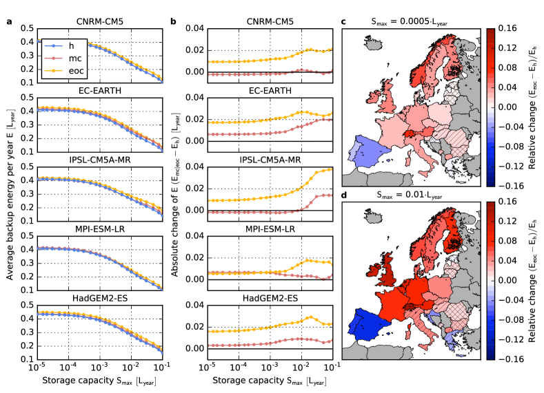
Figure 2: Impact of strong climate change on backup energy needs in Europe. a, Amount of energy that has to be provided by dispatchable backup generators in Germany as a function of the storage capacity $S_{\rm max}$ for the five models in the EURO-CORDEX ensemble and a strong climate change scenario (RCP8.5). Energy is given in units of the average yearly gross electricity consumption $L_{\rm year}$. Blue: 1970-2000 (h), Red: 2030-2060 (mc), Yellow: 2070-2100 (eoc). b, Absolute change of the average backup energy as a function of $S_{\rm max}$ in Germany. Colors are the same as in panel a. c, d, Relative change of the average backup energy needs by the end of the century with respect to the historical time frame for 29 European countries and two values of the storage capacity $S_{\rm max}$. The color code corresponds to the average of the five models and the hatching indicates the robustness of the results. No hatching: 5/5, striped: 4/5, crossbred: 3/5 models agree on the sign of change.

Increase of backup and storage needs

All models in the EURO-CORDEX ensemble predict an increase of the necessary backup energy in most of Central Europe (i.e. Germany, Poland, Czech Republic, Switzerland, Austria, the Netherlands and Belgium), France, the British Isles and Scandinavia for a strong climate change scenario (RCP8.5) by the end of the century relative to the historical time frame (see Fig. 2c and d). This implies that even though the same amount of energy is produced by renewables in both time frames, less renewable energy can actually be used. Relative changes are highest in Switzerland and the United Kingdom with a range between 12.2 to 24.2 % (mean: 15.6 %) and 7.1 to 16.5 % (mean: 12.1 %), respectively for a storage capacity of $S_{\rm max}=0.01\cdot L_{\rm year}$. However, results for mountainous regions like Switzerland should be regarded with caution as wind farms might be placed at sites which are unsuitable. In addition, climate model results over complex terrain are known to have large uncertainties. An opposite effect is observed for the Iberian Peninsula, Greece and Croatia where the need for backup energy decreases (e.g., Spain: -4.7 to -15.5 %; mean: -9.1 % for $S_{\rm max}=0.01\cdot L_{\rm year}$). These results hold for a variety of scenarios for the development of storage infrastructures leading to different values of the storage size $S_{\rm max}$, being more pronounced for larger storage sizes. The latter partly results from a change in the seasonal variability of the wind power generation (cf. below). In the Baltic region and South-Eastern Europe, relative changes are weaker and the models most often do not agree on the sign of change.

Similar changes are observed already at mid century (2030-2060, see Fig. S4 in Appendix B) and for RCP4.5 (see Fig. S7 in Appendix C). However, the results are less pronounced and often not robust (i.e. the models do not agree on the sign of change).

For Germany (Fig. 2a and b), the absolute increase of the average backup energy per year $E$ amounts to 0.6-3.8 % of the average yearly consumption $L_{\rm year}$ by the end of the century. Assuming a yearly consumption of the order of $L_{\rm year}=600$ TWh AGE2016 , this corresponds to an additional need of 4-23 TWh of backup energy per year.

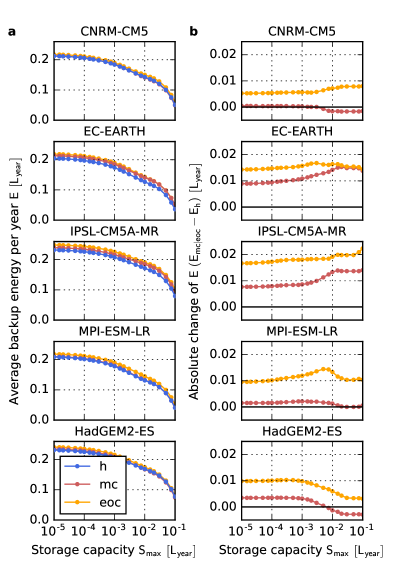
Figure 3: Impact of strong climate change on backup energy needs for a perfectly interconnected European power system. a, Amount of energy that has to be provided by dispatchable backup generators in Europe as a function of the storage capacity $S_{\rm max}$ for the five models in the EURO-CORDEX ensemble and a strong climate change scenario (RCP8.5). Energy is given in units of the average yearly gross electricity consumption $L_{\rm year}$. Blue: 1970-2000 (h), Red: 2030-2060 (mc), Yellow: 2070-2100 (eoc). b, Absolute change of the average backup energy as a function of $S_{\rm max}$. Colors are the same as in panel a.

In a perfectly interconnected Europe, the average relative backup energy per year is much smaller than for individual countries (e.g., for Germany, cf Fig. 2a and Fig. 3a). This is because the balancing takes place over a large spatial scale with many different wind patterns at the same time step. For all five models and all storage capacities, we find an increase of the average backup energy per year $E$ by the end of the century (see Fig. 3). Values range from 0.3 to 2.2 % of the average yearly consumption $L_{\rm year}$ corresponding to a relative change of 2.3 to 40.2 % ($(E_{\rm eoc}-E_{\rm h})/E_{\rm h}$). For high storage capacities, the change depends strongly on the seasonal wind variability (cf. below). For mid century, the same effect albeit at a weaker magnitude can be observed.

Two main drivers for the increase in the backup energy can be identified: a higher probability for long periods with low wind power generation and a higher seasonal wind variability.

Challenges by long low-wind periods

The backup energy need is particularly high during long periods with low renewable generation which cannot be covered by limited storage facilities. In Fig. 4 we show the duration distribution of periods for which wind power generation is continuously lower than average (i.e. $R(t)<\langle R\rangle$) for Germany (panel a) and the relative change of the 95 % quantile (panel b). The 95 % quantile shifts to longer durations in most of Central Europe, France, the British Isles, Sweden and Finland and decreases on the Iberian Peninsula by the end of the century. These findings are robust in the sense that all five models in the EURO-CORDEX ensemble agree on the sign of change as illustrated for Germany in Fig. 4a.

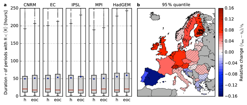
Figure 4: Change of the duration of periods with low wind generation. a, Distribution of the duration of periods during which the wind generation is continuously lower than average ($R(t)<\langle R\rangle$) in Germany for the five models in the EURO-CORDEX ensemble. Boxes represent the 25 % to 75 % quantiles, whiskers indicate the 5 % and 95 % quantiles, the red line is the median, the blue dot shows the mean and black dots represent outliers. Results are shown for the historical time frame (h, 1970-2000) and the end of the century (eoc, 2070-2100) for a strong climate change scenario (RCP8.5). b, Relative change of the duration assigned to the 95 % quantile by the end of the century with respect to the historical time frame for 29 European countries. The color code corresponds to the average of the five models and the hatching indicates the robustness of the results. No hatching: 5/5, striped: 4/5, crossbred: 3/5 models agree on the sign of change.

Long low-wind periods are crucially difficult for the operation of future renewable power systems Elsn15 . An increasing magnitude for such extreme events thus represents a serious challenge for renewable integration. In Eastern Europe, Italy, Greece and Norway relative changes are weaker and not robust. The effect develops mostly in the second half of the century (cf. Fig. S5 in Appendix B) and for strong climate change (RCP8.5, cf. Fig. S8 in Appendix C).

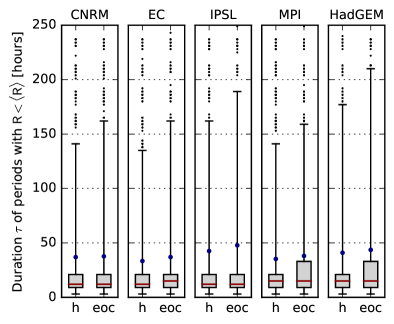
Figure 5: Change of the duration of periods with low wind generation for Europe as a whole. Distribution of the duration of periods during which the wind generation is continuously lower than average ($R(t)<\langle R\rangle$) in Europe for the five models in the EURO-CORDEX ensemble. Boxes represent the 25 % to 75 % quantiles, whiskers indicate the 5 % and 95 % quantiles, the red line is the median, the blue dot shows the mean and black dots represent outliers. Results are shown for the historical time frame (h, 1970-2000) and the end of the century (eoc, 2070-2100) for a strong climate change scenario (RCP8.5).

Considering the perfectly interconnected European power system (see Fig. 5), we find that the average duration of low-wind periods ($R(t)<\langle R\rangle$) and the 95 % quantile both shift to higher values by the end of the century. This indicates that long lasting low-wind conditions which extend over the whole European continent become more likely (also discussed in 2017Wohland ).

Higher seasonal wind variability

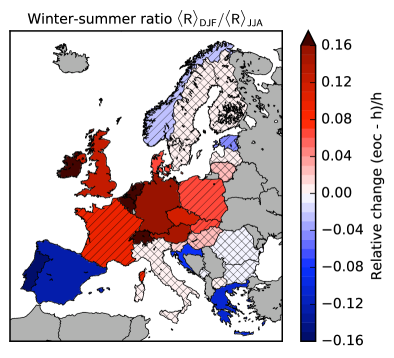
Figure 6: Impact of strong climate change on the seasonal variability of wind power generation. Relative change of the winter-summer ratio of the average wind power yield $\langle R\rangle_{\rm DJF}/\langle R\rangle_{\rm JJA}$ (DJF: December-February vs. JJA: June-August) by the end of the century (eoc, 2070-2100) with respect to the historical time frame (h, 1970-2000). The brackets denote the temporal average over the respective winter and summer months. Results are shown for a strong climate change scenario (RCP8.5) for 29 European countries. The color code corresponds to the average of the five models and the hatching indicates the robustness of the results. No hatching: 5/5, striped: 4/5, crossbred: 3/5 models agree on the sign of change.

The second reason for an increase of backup and storage needs is an increasing intensity of the seasonal wind variability. Typically, the wind power yield is highest in the winter months such that backup power plants are needed mostly in summer.

The winter-summer ratio increases for most of Central and North-Western Europe, and decreases for the Iberian Peninsula, Greece and Croatia (see Fig. 6) for four or all five models in the EURO-CORDEX ensemble. In these countries the seasonal variability therefore contributes to the observed changes of backup needs. Changes are small and not robust in Italy, most of Eastern Europe and Scandinavia (except Denmark). Hence, the increase of backup needs in Northern Europe is attributed solely to the higher probability for long periods with low wind power generation. For mid century (see Fig. S6 in Appendix B), and for medium climate change (RCP4.5, see Fig. S9 in Appendix C), results are comparable but less robust for some countries.

For the perfectly interconnected European power system, four of the five models predict an increasing seasonal wind variability in the range of 4.1 to 10.4 %. Thus, the lower seasonal wind variability on the Iberian Peninsula, Greece and Croatia cannot totally compensate the higher seasonal wind variability in the other European countries. In contrast, HadGEM2-ES predicts a decrease of -2.8 %.

The higher seasonal wind variability also explains the relative increase of the backup energy for higher storage capacities (cf. Fig. 2). A high storage capacity allows to store some part of the energy for several months. However, as the storage capacity is still limited, a higher seasonal wind variability implies that the storage is fully charged earlier in winter and that it is depleted earlier in summer. Thus, less excess energy can be transferred from the winter to the summer months if the seasonal variability of wind power generation increases.

Low-wind periods in a large CMIP5 ensemble

To substantiate our findings, we analyze a large CMIP5 ensemble Tayl12 consisting of 22 GCMs with a much coarser resolution than the EURO-CORDEX ensemble as explained in the methods section.

The typical duration of periods with $f(t)\leq f_{\rm th}$ in Central Europe increases by the end of the century for most GCMs in the CMIP5 ensemble. 19 of the 22 models predict an increase of the mean duration (Fig. 7b). The 90 % quantile of the duration increases for 16 models and remains unchanged for the remaining six models, while the 95 % quantile increases for 18 of the 22 models. Fig. 7b shows that the five models of the EURO-CORDEX ensemble (shown as filled circles) form a representative subset of the CMIP5 ensemble since their results are well distributed within the range of the majority of all models and thus do not contain outliers. Hence, the large CMIP5 ensemble corroborates our previous findings, predicting an increase of the likelihood for long periods with low wind power output for a strong climate change scenario.

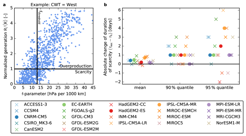
Figure 7: Assessment of long low-wind periods in a large CMIP5 ensemble. a, Days with below average wind power generation in Central Europe are identified by a low value of the $f$-parameter ($f(t)\leq f_{\rm th}$) in the GCM output. To determine the optimal value of the threshold $f_{\rm th}$, for each circulation weather type (CWT, here, the western type is shown) we compare the $f$-parameter to the German wind power output $R(t)$, calculated from the dynamically downscaled ERA-Interim reanalysis dataset dee11 . b, Absolute change of the duration of periods with $f(t)\leq f_{\rm th}$ by the end of the century (eoc, 2070-2100) compared to the historical time frame (h, 1970-2000) for a strong climate change scenario (RCP8.5) for 22 GCMs in the CMIP5 ensemble. The change of the mean duration, the 90 % quantile and the 95 % quantile of the duration distribution are shown. Filled circles represent the five GCMs which are also downscaled by the EURO-CORDEX initiative.

To assess the sensitivity of the choice of $f_{\rm th}$, we repeated our analysis by determining one value for $f_{\rm th}$ which is independent of the underlying CWT. This does not change the results as shown in Fig. S16 in Appendix D.

Climatologic developments driving enhanced seasonality

The identified increase in the seasonal variability of wind power generation has been discussed in terms of the projected changes of large-scale atmospheric circulation and regional wind conditions. A consensus exists about general changes in the large-scale circulation patterns in the Eastern North Atlantic region and Europe, which is however dependent on the time of the year Demu09 . During winter, the eddy-driven jet stream and cyclone intensity are extended towards the British Isles Woll12 . Accordingly, winter storminess is projected to increase over Western Europe Pint12 ; Fese15 , leading to enhanced winds over Western and Central Europe. The signal in summer corresponds rather to a northward shift of the eddy driven jet stream, cyclone activity and lower tropospheric winds, together with an increase in anticyclonic circulation over Southern Europe Zapp15 . The latter is associated with an expansion of the Hadley circulation due to enhanced radiative forcing Lu07 . These developments are projected to decrease wind speeds during summer hueg13 ; Reye15 ; Reye16 ; 2017Moemken .

These seasonal changes have strong implications not only on temperature and precipitation patterns, but also in the seasonal wind regimes and intra-annual variability. The seasonal variability of wind power generation increases under future climate conditions Reye15 ; hueg13 ; 2017Moemken even though the annual mean changes are comparatively small Tobi15 ; Tobi16 ; Reye16 ; hueg13 ; 2017Moemken . The impact may be large for the operational systems, and thus needs to be quantified adequately based on state-of-the-art climate model projections. For future research it would thus be highly desirable to provide larger ensembles of dynamically downscaled models for various regions on earth, possibly including wind speeds at hub heights.

Discussion

Wind power, PV and other renewable sources can satisfy the majority of the global energy demand Jacobson11 ; Sims11 ; Lu09 . However, system integration remains a huge challenge: The operation of wind turbines and PV relies on weather and climate and thus shows strong temporal fluctuations olau16 ; davi16 ; Heid10 ; Elsn15 ; diaz12 ; Schlachtb16 ; Bloo16 ; Hube14 ; Grams17 . The impact of climate change on the global energy yields of wind and solar power has been addressed previously Tobi15 ; Tobi16 ; Reye15 ; Reye16 ; 2017Moemken ; Jere15 , but the impact on fluctuations and system integration has remained unconsidered.

In this paper, we analyzed the change of the temporal characteristics of wind power generation in a strong (RCP8.5) and a medium climate change scenario (RCP4.5, see Appendix C). Backup and storage needs increase in most of Central, Northern and North-Western Europe and decrease over the Iberian Peninsula, Greece and Croatia. As these effects are observed for both aggregation approaches used in this study (approach (a): aggregation per country, approach (b): European copperplate), we hypothesize that the effect will also be observed in intermediate scenarios with restricted interconnection between countries. Two main climatologic reasons for the observed increase were identified: a higher probability for long periods of low wind power generation and a stronger seasonal wind variability. The same tendencies, albeit at a different magnitude, are observed for different renewable penetrations, load time series and siting of wind turbines (see Appendix D).

The projected increase in backup energy needs may partly be compensated by using an appropriate mix of wind and PV. Furthermore, wind generation from offshore wind farms is often more persistent and installed capacities are strongly increasing. In a further study, climate projections for onshore and offshore wind and PV should thus be analyzed together in order to account for possible changes in the temporal variations of the combined system of renewables.

To isolate the change of the temporal characteristics of wind power generation, we made several simplifications. First of all, we assumed that wind provides a fixed share of the load for all time frames. This procedure normalizes out a possible change of global wind yields (already discussed in Tobi15 ; Tobi16 ; Reye15 ; Reye16 ; 2017Moemken ). Technological progress of the wind turbines and changes of typical hub heights were not considered. For an integrated assessment, these aspects should be taken into account, but our approach reveals the impact of climate change on the temporal characteristics clearly.

A reliable interpretation of climate projections should be based on multi-model ensembles Tayl12 ; Tobi16 . Our analysis of the small EURO-CORDEX ensemble consisting of five models shows robust results regarding the sign of change for several regions in Europe. A statistical analysis of the output of 22 GCMs from the CMIP5 ensemble supports our findings, as the duration of periods with low values of the $f$-parameter over Central Europe is likely to increase. Large-scale climatologic developments leading to an increase of the seasonal wind variability were previously discussed in Demu09 ; Woll12 ; Zapp15 ; Lu07 ; Pint12 ; Fese15 ; hueg13 ; Reye15 ; 2017Moemken . For future research, it would be highly desirable if larger ensembles of dynamically downscaled models would be provided. Furthermore, data at turbine hub height should be made available. Ongoing downscaling experiments within the new CMIP6 CORDEX initiative Eyri16 will allow to assess the impact of climate change on system integration of intermittent renewables for various regions in the same manner. This should include a detailed and explicit analysis on the projected changes of both wind and PV. In conclusion, our work contributes to highlight the importance of integrated energy and climate research to enable a sustainable energy transition.

Appendix
accompanying the manuscript
Impact of climate change on backup energy and storage needs in wind-dominated power systems in Europe
Juliane Weber, Jan Wohland, Mark Reyers, Julia Moemken, Charlotte Hoppe, Joaquim G. Pinto and Dirk Witthaut

Appendix A Supporting material for the methods section

Table S1: Global circulation models used in the EURO-CORDEX ensemble. The downscaled data has a resolution of 0.11^∘ and 3 hours Jaco14 . Table adapted from Reye16

Model name	Institution
CNRM-CM5 (CNRM Coupled Global Climate Model, version 5)	Centre National de Recherches Météorologiques (CNRM), France
EC-EARTH (EC-Earth Consortium)	European Consortium (EC)
IPSL-CM5A-MR (IPSL Coupled Model, version 5, coupled with NEMO, medium resolution)	Institut Pierre Simon Laplace (IPSL), France
MPI-ESM-LR (MPI Earth System Model, low resolution)	Max Planck Institute (MPI) for Meteorology, Germany
HadGEM2-ES (Hadley Centre Global Environment Model, version 2, Earth System)	Met Office Hadley Centre, United Kingdom

Appendix B Mid century (2030-2060)

In the main manuscript, most results are only shown for the end of the century (2070-2100). Here, results shall be shown for mid century (2030-2060).

In Fig. S4 the relative change of the backup energy is shown for two different storage capacities. For most of Central Europe, France, the British Isles, Scandinavia (except Denmark) and Italy four to five models in the EURO-CORDEX ensemble predict an increasing backup need. Exceptions are Germany, where results are not robust for small $S_{\rm max}$ and Norway, Sweden, Poland and the Czech Republic, where results are not robust for high $S_{\rm max}$. For Spain, Greece and Croatia (and Portugal for high $S_{\rm max}$) four models predict a slightly decreasing backup need. Compared to the results we have for the end of the century (cf. Fig 2c and d in the main manuscript), changes are weaker and, therefore, in some countries less robust. For most countries in Eastern Europe results are not robust which is also observed for the end of the century.

The duration distribution of periods with $R(t)<\langle R\rangle$ and the relative change of the 95 % quantile of this distribution are shown in Fig. S5. In almost all European countries the five models do not agree on the sign of change. These results indicate that changes in the backup energy need can mostly not be attributed to a change in the duration of long low wind periods.

Instead, higher/lower backup needs can be explained by the winter-summer ratio (see Fig. S6) which is predicted to increase in France, the British Isles, and most of Central Europe (except Germany) by four to five models. Furthermore, the ratio is predicted to decrease on the Iberian Peninsula, Greece and (not robustly) in the Baltic countries. The relative change, however, is lower than by the end of the century (cf. Fig 6 in the main manuscript).

Hence, by mid century, there is still a trend for increasing backup and storage needs due to a change in the seasonal wind variability. However, relative changes are weaker and results are less robust for some countries.

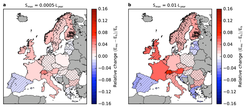
Figure S4: Impact of strong climate change on backup energy needs by mid century. Parameters and presentation as in Fig. 2.

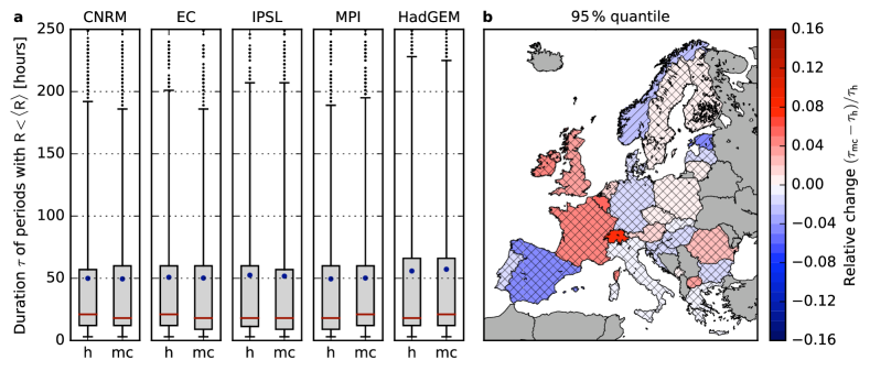
Figure S5: Change of the duration of periods with low wind generation by mid century. Parameters and presentation as in Fig. 4.

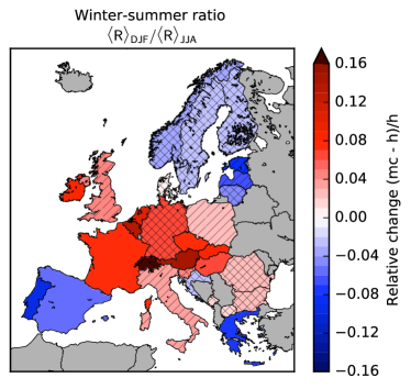
Figure S6: Impact of strong climate change on the seasonal variability of wind power generation by mid century. Parameters and presentation as in Fig. 6.

Appendix C RCP4.5

We repeated the analysis for the medium climate change scenario RCP4.5 which is leading to an increase of 4.5 W/m² in radiative forcing ($\sim$650 ppm CO₂ equivalent) by 2100 Vuur11 . Fig. S7 shows the impact of this scenario on backup energy needs in Germany (panels a and b) and Europe (panels c and d) by the end of the century (2070-2100). The backup need increases in most of Central Europe, France and the British Isles. Even though the increase is weaker than in the RCP8.5 scenario (cf. Fig 2 in the main manuscript), it is important to note that the effect on the backup need is still pronounced in most of these countries. For France, Belgium, Scandinavia, Italy and Poland, the robustness of the results depends on the storage size. As for RCP8.5, results are not robust in most of Eastern Europe. The decrease in the backup need on the Iberian Peninsula (for high $S_{\rm max}$), Greece and Croatia is not robust.

The increase in the backup need can only partly be explained by an increase in the duration of long low wind periods (see Fig. S8). Only in Switzerland and Belgium all models agree on the sign of change and on the British Isles, France, Austria and the Czech Republic, four of the five models agree on the sign of change. In the other countries, results are not robust and/or relative changes are small.

Changes in the backup need can mostly be explained by changes in the winter-summer ratio (see Fig. S9): For those countries, in which the backup energy need increases, the winter-summer ratio also increases (the British Isles, Benelux, France, Switzerland, Austria, Czech, Slovakia, Slovenia, Germany and Italy).

In conclusion, by the end of the century similar trends as in the RCP8.5 scenario are found using the RCP4.5 scenario. However, changes are weaker and, therefore, often less robust. The decreasing backup needs on the Iberian Peninsula, Greece and Croatia are not robust for medium climate change.

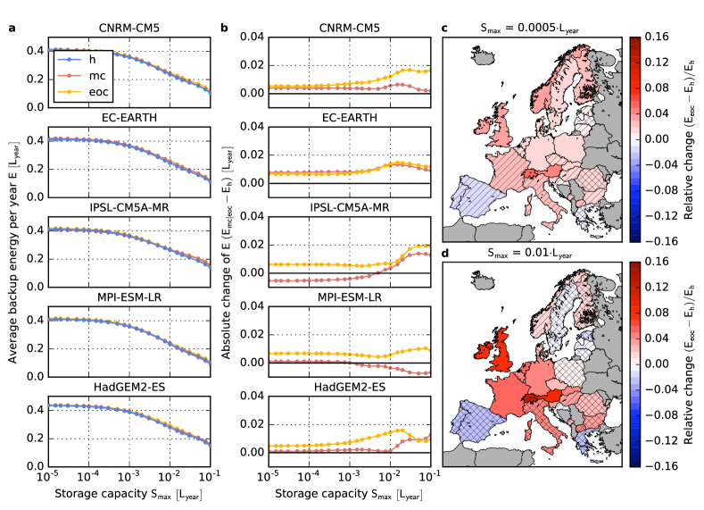
Figure S7: Impact of medium climate change on backup energy needs in Europe. Parameters and presentation as in Fig. 2.

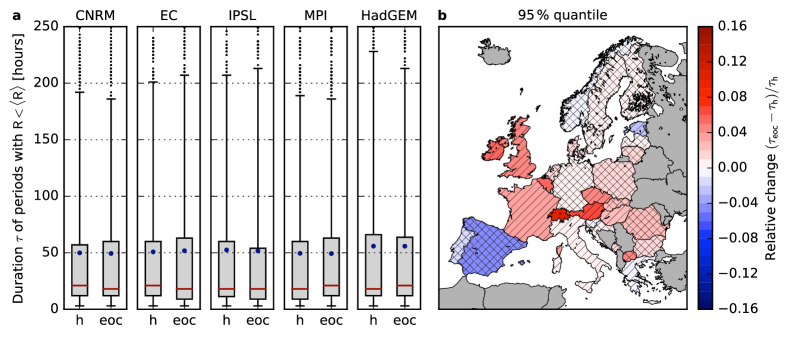
Figure S8: Change of the duration of periods with low wind generation for a medium climate change scenario. Parameters and presentation as in Fig. 4.

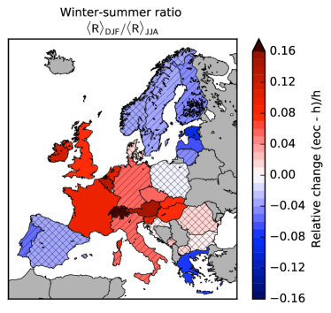
Figure S9: Impact of medium climate change on the seasonal variability of wind power generation. Parameters and presentation as in Fig. 6.

Appendix D Sensitivity studies

In order to examine the sensitivity of our system on different parameters, we repeated our analysis using (a) different penetrations of renewables: $\gamma=1.2$ and $\gamma=0.8$, Rasm12 , (b) a constant load entsoe_load and (c) a different distribution of wind farms. Furthermore, we repeated the analysis of the CMIP5 ensemble by using one threshold value of the $f$-parameter ($f_{\rm th}$) for all circulation weather types to characterize periods of low wind power generation.

Renewable penetration

Different penetrations of wind power are simulated by scaling the renewable generation using the $\gamma$ factor: $\langle R\rangle=\gamma\,\langle L\rangle$. In the case $\gamma<1$, on average an energy amount of $(1-\gamma)\cdot L_{\rm year}$ has to be provided by non-renewable power plants. Thus, we are interested in the additional backup energy $E_{\rm add}=E-(1-\gamma)\cdot L_{\rm year}$ with $E=\langle B\rangle/\langle L\rangle\cdot L_{\rm year}$.

In Figs S10 and S11 the change in the backup energy need is shown for $\gamma=1.2$ and $\gamma=0.8$, respectively. A comparison with Fig 2 of the main manuscript shows that absolute values of the backup energy (panels a) decrease (as expected). However, the absolute change of the backup energy (panels b) is quite similar and, thus, the relative change (panels c and d) is even higher for most countries (e.g. for UK the average relative change is 36.2 % for $\gamma=0.8$ and 20.2 % for $\gamma=1.2$ for $S_{\rm max}=0.01\cdot L_{\rm year}$). For all countries, the average predicted sign of change is the same as for $\gamma=1$. Less models agree an the sign of change only in the case of Spain, Greece and Croatia (only high $S_{\rm max}$) for $\gamma=0.8$ compared to $\gamma=1$.

Hence, a higher or lower renewable penetration also leads to increasing (decreasing) backup needs in many European countries, often even with higher relative changes.

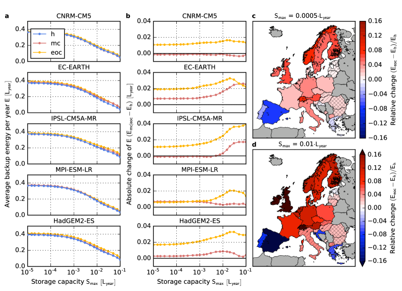
Figure S10: Impact of strong climate change on backup energy needs in Europe for a renewable penetration of $\mathbf{\boldsymbol{\gamma}=1.2}$. The maximum relative changes are 0.20 in Switzerland and -0.18 in Spain. Further parameters and presentation as in Fig. 2.

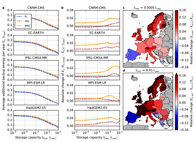
Figure S11: Impact of strong climate change on backup energy needs in Europe for a renewable penetration of $\mathbf{\boldsymbol{\gamma}=0.8}$. Shown is the amount of energy that has additionally to the pre-defined 20 % to be provided by dispatchable backup generators. The maximum relative change is 0.36 in UK. Further parameters and presentation as in Fig. 2.

Different load time series

In order to analyze the sensitivity of the results on the applied load time series, we repeated our analysis using a constant value for the load such that: $L=\langle R\rangle$. The change of the backup energy need is shown in Fig. S12. A comparison with Fig 2 of the main manuscript reveals that the dependence of the results on the exact load time series is weak. Absolute values of the backup energy increase slightly (panels a). This comes from the fact that using a constant load leads to a loss of positive correlations: On average, there is more wind generation in winter than in summer. This correlates to a higher electricity demand in winter than in summer (in many countries). However, the relative change of the backup energy need is hardly affected. Only in Finland and Norway less models agree on the sign of change in the case of high $S_{\rm max}$.

Thus, we find only a weak dependence of the results on the exact load time series. This can further be explained by the fact that the fluctuations in the wind generation are much higher than fluctuations in the demand (cf. Fig 1c in the main manuscript) in scenarios with high wind penetrations.

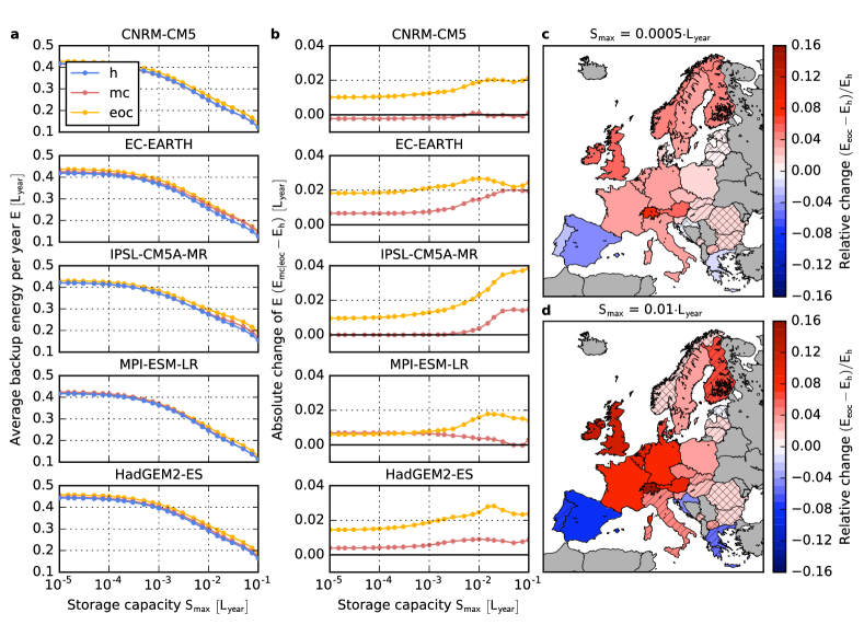
Figure S12: Impact of strong climate change on backup energy needs in Europe for a constant load. Parameters and presentation as in Fig. 2.

Different distribution of wind farms

In order to quantify the importance of the exact placement of wind farms, we repeated the analysis assuming a homogeneous distribution of wind farms at each grid point within a country.

A comparison of Fig. S13 with Fig 2 of the main manuscript shows that absolute backup energy values slightly increase (panels a). This is because wind farms are sited on less windy locations on average. However, the relative change of the backup energy hardly depends on the exact wind farm distribution. For Portugal and Greece results become more robust (for high $S_{\rm max}$) whereas in Croatia results become less robust.

For Germany, the duration distribution of periods with $R(t)<\langle R\rangle$ is shifted to higher values for a homogeneous distribution of wind farms (cf. Fig. S14 and Fig 4 in the main manuscript, panels a) because wind farms are sited less favorable. Regarding the relative change of the 95 % quantile of the duration distribution (panels b), results are less robust in Sweden, Austria, Estonia, Portugal and Slovenia whereas in Italy, Denmark, Greece and Latvia more models agree on the sign of change. In Italy, the sign of change flips – the duration of long periods with low wind power output tends to decrease. In all other countries, especially in Central Europe, France and the British Isles the qualitative results are the same.

The relative change of the winter-summer ratio is more pronounced if wind farms are placed homogeneously on each grid point within a country (cf. Fig. S15 with Fig 6 in the main manuscript; be aware that the scales of the colorbars are different). The sign of change is the same in all countries. In Croatia and Slovakia results become less robust whereas in Finland and Lithuania more robust results are revealed.

All in all, the exact distribution of wind farms does hardly alter the results reported in this study (except for Italy).

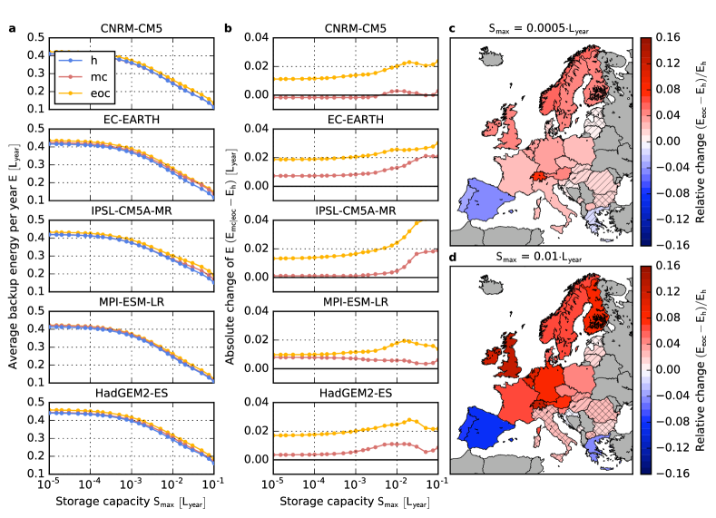
Figure S13: Impact of strong climate change on backup energy needs in Europe for a homogeneous distribution of wind farms. Parameters and presentation as in Fig. 2.

Figure S14: Change of the duration of periods with low wind generation for a homogeneous distribution of wind farms. Parameters and presentation as in Fig. 4.

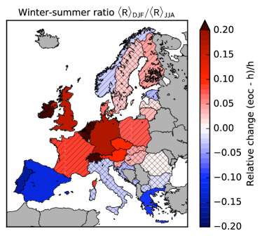
Figure S15: Impact of strong climate change on the seasonal variability of wind power generation for a homogeneous distribution of wind farms. Parameters and presentation as in Fig 6. Be aware that the scale of the colorbar is different than in Fig. 6.

Repetition of the analysis of the CMIP5 ensemble using a different threshold value of the $f$-parameter

In the main manuscript, we determined the duration of periods with low wind generation by deriving one threshold value $f_{\rm th}$ for each CWT. It is important to note that the determined threshold value $f_{\rm th}$ is not perfect, as the distance $(1-{\rm SEN})^{2}+{\rm FFP}^{2}$ is far away from being zero (see red dot in Fig C in S1_Appendix). Hence, there is still a certain amount (for the western CWT: 19 %) of false predictions. Thus, the derived duration distribution depends on the choice of the threshold value $f_{\rm th}$. To assess the sensitivity of the choice of $f_{\rm th}$, we repeat our analysis by determining one value for $f_{\rm th}$ which is independent of the underlying CWT. The result is shown in Fig. S16. A comparison to Fig 7b in the main manuscript shows that in both cases the ensemble of the 22 GCMs predicts the same: The mean, the 90 % quantile and the 95 % quantile tend to increase by the end of the century. However, the value of a single model may be shifted for the 90 % quantile and the 95 % quantile: E.g. for HadGEM2-ES the absolute change of the duraton of scarcity of the 90 % quantile is one day in Fig 7b and two days in Fig. S16. An explanation for this is that already a slight shift of the threshold value $f_{\rm th}$ can split one long period with $f(t)\leq f_{\rm th}$ into two shorter periods with $f(t)\leq f_{\rm th}$ and a short period with $f(t)>f_{\rm th}$ in between or vice versa. Therefore, the results for the extremes (i.e. the 90 % quantile and the 95 % quantile) may be shifted for a single model. This effect averages out over the ensemble.

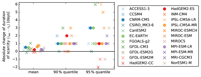
Figure S16: Absolute change of the duration of periods with low wind generation using one $f_{\rm th}$ for all CWTs. Parameters and presentation as in Fig. 7b.

References

- (1) T. Bruckner et al. Energy systems. In O. Edenhofer et al. (ed.) Climate Change 2014: Mitigation of Climate Change. Contribution of Working Group III to the Fifth Assessment Report of the Intergovernmental Panel on Climate Change (Cambridge University Press, Cambridge, United Kingdom, 2014).
- (2) UNFCCC. Adoption of the Paris Agreement. Report No. FCCC/CP/2015/L.9/Rev.1. http://unfccc.int/resource/docs/2015/cop21/eng/l09r01.pdf (2015).
- (3) Rogelj, J. et al. Energy system transformations for limiting end-of-century warming to below 1.5∘C. Nature Climate Change 5, 519–527 (2015).
- (4) Rogelj, J. et al. Paris agreement climate proposals need a boost to keep warming well below 2∘C. Nature 534, 631–639 (2016).
- (5) Jacobson, M. Z. & Delucchi, M. A. Providing all global energy with wind, water, and solar power, Part I: Technologies, energy resources, quantities and areas of infrastructure, and materials. Energy Policy 39, 1154–1169 (2011).
- (6) R. Sims et al. Integration of renewable energy into present and future energy systems. In O. Edenhofer et al. (ed.) IPCC Special Report on Renewable Energy Sources and Climate Change Mitigation (Cambridge University Press, Cambridge, United Kingdom, 2011).
- (7) Bloomfield, H., Brayshaw, D. J., Shaffrey, L. C., Coker, P. J. & Thornton, H. Quantifying the increasing sensitivity of power systems to climate variability. Environmental Research Letters 11, 124025 (2016).
- (8) Olauson, J. et al. Net load variability in Nordic countries with a highly or fully renewable power system. Nature Energy 1, 16175 (2016).
- (9) Davidson, M. R., Zhang, D., Xiong, W., Zhang, X. & Karplus, V. J. Modelling the potential for wind energy integration on China’s coal-heavy electricity grid. Nature Energy 1, 16086 (2016).
- (10) Huber, M., Dimkova, D. & Hamacher, T. Integration of wind and solar power in Europe: Assessment of flexibility requirements. Energy 69, 236–246 (2014).
- (11) Weber, J., Zachow, C. & Witthaut, D. Modeling long correlation times using additive binary markov chains: applications to wind generation time series. arXiv preprint arXiv:1711.03294 (2017).
- (12) Heide, D. et al. Seasonal optimal mix of wind and solar power in a future, highly renewable Europe. Renewable Energy 35, 2483 (2010).
- (13) Elsner, P., Fischedick, M. & Sauer, D. U. Flexibilitätskonzepte für die Stromversorgung 2050 (Acatech, Muenchen, 2015).
- (14) Díaz-González, F., Sumper, A., Gomis-Bellmunt, O. & Villafáfila-Robles, R. A review of energy storage technologies for wind power applications. Renewable and Sustainable Energy Reviews 16, 2154–2171 (2012).
- (15) Van Vliet, M. T. et al. Vulnerability of US and European electricity supply to climate change. Nature Climate Change 2, 676–681 (2012).
- (16) Van Vliet, M. T., Wiberg, D., Leduc, S. & Riahi, K. Power-generation system vulnerability and adaptation to changes in climate and water resources. Nature Climate Change 6, 375–380 (2016).
- (17) Allen, M. R., Fernandez, S. J., Fu, J. S. & Olama, M. M. Impacts of climate change on sub-regional electricity demand and distribution in the southern united states. Nature Energy 1, 16103 (2016).
- (18) Auffhammer, M., Baylis, P. & Hausman, C. H. Climate change is projected to have severe impacts on the frequency and intensity of peak electricity demand across the united states. Proceedings of the National Academy of Sciences 114, 1886–1891 (2017).
- (19) Pryor, S. & Barthelmie, R. Climate change impacts on wind energy: a review. Renewable and sustainable energy reviews 14, 430–437 (2010).
- (20) Tobin, I. et al. Assessing climate change impacts on European wind energy from ENSEMBLES high-resolution climate projections. Climatic Change 128, 99–112 (2015).
- (21) Tobin, I. et al. Climate change impacts on the power generation potential of a European mid-century wind farms scenario. Environmental Research Letters 11, 034013 (2016).
- (22) Reyers, M., Pinto, J. G. & Moemken, J. Statistical–dynamical downscaling for wind energy potentials: evaluation and applications to decadal hindcasts and climate change projections. International Journal of Climatology 35, 229–244 (2015).
- (23) Reyers, M., Moemken, J. & Pinto, J. G. Future changes of wind energy potentials over Europe in a large CMIP5 multi-model ensemble. International Journal of Climatology 36, 783–796 (2016).
- (24) Moemken, J., Reyers, M., Feldmann, H. & Pinto, J. G. Wind speed and wind energy potentials in EURO-CORDEX ensemble simulations: evaluation and future changes. Journal of Geophysical Research: Atmospheres (submitted) .
- (25) Jerez, S. et al. The impact of climate change on photovoltaic power generation in Europe. Nature Communications 6, 10014 (2015).
- (26) Stanton, M. C. B., Dessai, S. & Paavola, J. A systematic review of the impacts of climate variability and change on electricity systems in Europe. Energy 109, 1148–1159 (2016).
- (27) Demuzere, M., Werner, M., Van Lipzig, N. & Roeckner, E. An analysis of present and future ECHAM5 pressure fields using a classification of circulation patterns. International Journal of Climatology 29, 1796–1810 (2009).
- (28) Woollings, T., Gregory, J. M., Pinto, J. G., Reyers, M. & Brayshaw, D. J. Response of the North Atlantic storm track to climate change shaped by ocean-atmosphere coupling. Nature Geoscience 5, 313–317 (2012).
- (29) Zappa, G., Hoskins, B. J. & Shepherd, T. G. Improving climate change detection through optimal seasonal averaging: the case of the North Atlantic jet and European precipitation. Journal of Climate 28, 6381–6397 (2015).
- (30) Lu, J., Vecchi, G. A. & Reichler, T. Expansion of the Hadley cell under global warming. Geophysical Research Letters 34 (2007).
- (31) Pinto, J. G., Karremann, M. K., Born, K., Della-Marta, P. M. & Klawa, M. Loss potentials associated with European windstorms under future climate conditions. Climate Research 54, 1–20 (2012).
- (32) Feser, F. et al. Storminess over the North Atlantic and northwestern Europe – a review. Quarterly Journal of the Royal Meteorological Society 141, 350–382 (2015).
- (33) Hueging, H., Haas, R., Born, K., Jacob, D. & Pinto, J. G. Regional changes in wind energy potential over Europe using regional climate model ensemble projections. Journal of Applied Meteorology and Climatology 52, 903–917 (2013).
- (34) Jacob, D. et al. EURO-CORDEX: new high-resolution climate change projections for European impact research. Regional Environmental Change 14, 563–578 (2014).
- (35) Giorgi, F. & Gutowski Jr, W. J. Regional dynamical downscaling and the CORDEX initiative. Annual Review of Environment and Resources 40, 467–490 (2015).
- (36) Taylor, K. E., Stouffer, R. J. & Meehl, G. A. An overview of CMIP5 and the experiment design. Bulletin of the American Meteorological Society 93, 485–498 (2012).
- (37) Jones, P., Hulme, M. & Briffa, K. A comparison of Lamb circulation types with an objective classification scheme. International Journal of Climatology 13, 655–663 (1993).
- (38) Dee, D. et al. The ERA-Interim reanalysis: Configuration and performance of the data assimilation system. Quarterly Journal of the royal meteorological society 137, 553–597 (2011).
- (39) Van Vuuren, D. P. et al. The representative concentration pathways: an overview. Climatic change 109, 5–31 (2011).
- (40) ESGF (Earth System Grid Federation) node at DKRZ (German Climate Computing Centre). EURO-CORDEX data. https://esgf-data.dkrz.de/projects/esgf-dkrz/ (accessed August 16, 2016).
- (41) Strandberg, G. et al. CORDEX scenarios for Europe from the Rossby Centre regional climate model RCA4 (SMHI, Sveriges Meteorologiska och Hydrologiska Institut, 2015).
- (42) Samuelsson, P. et al. The Rossby Centre Regional Climate model RCA3: model description and performance. Tellus A 63, 4–23 (2011).
- (43) Manwell, J. F., McGowan, J. G. & Rogers, A. L. Wind Energy Explained (John Wiley & Sons, Ltd, 2009).
- (44) Andresen, G. B., Søndergaard, A. A. & Greiner, M. Validation of Danish wind time series from a new global renewable energy atlas for energy system analysis. Energy 93, 1074–1088 (2015).
- (45) Monforti, F., Gaetani, M. & Vignati, E. How synchronous is wind energy production among European countries? Renewable and Sustainable Energy Reviews 59, 1622–1638 (2016).
- (46) Rodriguez, R. A., Becker, S., Andresen, G. B., Heide, D. & Greiner, M. Transmission needs across a fully renewable European power system. Renewable Energy 63, 467–476 (2014).
- (47) Schlachtberger, D., Becker, S., Schramm, S. & Greiner, M. Backup flexibility classes in emerging large-scale renewable electricity systems. Energy Conversion and Management 125, 336–346 (2016).
- (48) Wohland, J., Reyers, M., Weber, J. & Witthaut, D. More homogeneous wind conditions under strong climate change decrease the potential for inter-state balancing of electricity in europe. Earth System Dynamics Discussions, https://doi.org/10.5194/esd-2017-48, in review (2017).
- (49) European Network of Transmission System Operators for Electricity (ENTSO-E). Hourly load values. https://www.entsoe.eu/db-query/consumption/mhlv-all-countries-for-a-specific-month (accessed December 10, 2016).
- (50) Rasmussen, M. G., Andresen, G. B. & Greiner, M. Storage and balancing synergies in a fully or highly renewable pan-European power system. Energy Policy 51, 642–651 (2012).
- (51) Jensen, T. V. & Greiner, M. Emergence of a phase transition for the required amount of storage in highly renewable electricity systems. The European Physical Journal Special Topics 223, 2475–2481 (2014).
- (52) Egan, J. P. Signal detection theory and ROC analysis (Academic Press, Cambridge, 1975).
- (53) AG Energiebilanzen e.V. Energieverbrauch in Deutschland im Jahr 2016. http://www.ag-energiebilanzen.de/ (2017).
- (54) Lu, X., McElroy, M. B. & Kiviluoma, J. Global potential for wind-generated electricity. Proceedings of the National Academy of Sciences 106, 10933–10938 (2009).
- (55) Grams, C. M., Beerli, R., Pfenninger, S., Staffell, I. & Wernli, H. Balancing Europe’s wind-power output through spatial deployment informed by weather regimes. Nature Climate Change 7, 557–562 (2017).
- (56) Eyring, V. et al. Overview of the Coupled Model Intercomparison Project Phase 6 (CMIP6) experimental design and organization. Geoscientific Model Development 9, 1937–1958 (2016).