$(2+1)$-dimensional interface dynamics: mixing time, hydrodynamic limit and Anisotropic KPZ growth

Abstract.

Stochastic interface dynamics serve as mathematical models for diverse time-dependent physical phenomena: the evolution of boundaries between thermodynamic phases, crystal growth, random deposition… Interesting limits arise at large space-time scales: after suitable rescaling, the randomly evolving interface converges to the solution of a deterministic PDE (hydrodynamic limit) and the fluctuation process to a (in general non-Gaussian) limit process. In contrast with the case of $(1+1)$-dimensional models, there are very few mathematical results in dimension $(d+1),d\geq 2$. As far as growth models are concerned, the $(2+1)$-dimensional case is particularly interesting: Wolf [45] conjectured the existence of two different universality classes (called KPZ and Anisotropic KPZ), with different scaling exponents. Here, we review recent mathematical results on (both reversible and irreversible) dynamics of some $(2+1)$-dimensional discrete interfaces, mostly defined through a mapping to two-dimensional dimer models. In particular, in the irreversible case, we discuss mathematical support and remaining open problems concerning Wolf’s conjecture [45] on the relation between the Hessian of the growth velocity on one side, and the universality class of the model on the other.

2010 Mathematics Subject Classification: 82C20, 60J10, 60K35, 82C24

Keywords: Interacting particle systems, Dimer model, Interface growth, Hydrodynamic limit, Anisotropic KPZ equation, Stochastic Heat Equation

1. Introduction

Many phenomena in nature involve the evolution of interfaces. A first example is related to phenomena of deposition on a substrate, in which case the interface is the boundary of the deposed material: think for instance of crystal growth by molecular beam epitaxy or, closer to everyday experience, of the growth of a layer of snow during snowfall (see e.g. [1] for a physicist’s introduction to growth phenomena). Another example is the evolution of the boundary between two thermodynamic phases of matter. Think of a block of ice immersed in water: the shape of the ice block, hence the water/ice boundary, changes with time and of course the dynamics is very different according to whether temperature is above, below or exactly at $0$ ^∘C.

A common feature of these examples is that on macroscopic (i.e. large) scales the interface evolution appears to be deterministic, while a closer look reveals that the interface is actually rough and presents seemingly random fluctuations (this is particularly evident in the snow example, since snowflakes have a visible size).

To try to model mathematically such phenomena, a series of simplifications are adopted. First, the so-called effective interface approximation: the $d$-dimensional interface in $(d+1)$-dimensional space is modeled as a height function $h:x\in\mathbb{R}^{d}\mapsto h_{x}(t)\in\mathbb{R}$, where $h_{x}(t)$ gives the height of the interface above point $x$ at time $t$ (think of $d=2$ in the case of snow falling on your garden, but $d=1$ for instance for snow falling and sliding down on your car window). This approximation implies that one ignores the presence of overhangs in the interface. (More often than not, the model is discretized and $\mathbb{R}^{d},\mathbb{R}$ are replaced by $\mathbb{Z}^{d},\mathbb{Z}$.) Secondly, in the usual spirit of statistical mechanics, the complex phenomena leading to microscopic interface randomness (e.g. chaotic motion of water molecules in the case of the ice/water boundary, or the various atmospheric phenomena determining the motion of individual snowflakes) are simplified into a probabilistic description where the dynamics of the height function is modeled by a Markov chain with simple, “local”, transition rules.

We already mentioned that on macroscopic scales the interface evolution looks deterministic: this means that rescaling space as $\epsilon^{-1}x$, height as $\epsilon h$ and time as $\epsilon^{-\alpha}t$ (we will discuss the scaling exponent $\alpha>0$ later) and letting $\epsilon\to 0$, the random function $\epsilon h_{\epsilon^{-1}x}(\epsilon^{-\alpha}t)$ converges to a deterministic function $\phi(x,t)$ that in general is the solution of a certain non-linear PDE. This is called the hydrodynamic limit and is the analog of a law of large numbers for the sum of independent random variables. When we say that convergence holds, it does not mean it is easy to prove it or even to write down the PDE explicitly. Indeed, as discussed in more detail in the following sections, above dimension $(d+1)=(1+1)$ the hydrodynamic limit has been proved only for a handful of models, and one of the goals of this review is to report on recent results for $d=2$.

On a finer scale, the interface fluctuations around the hydrodynamic limit are expected to converge, after proper rescaling, to a limit stochastic process, not necessarily Gaussian. In some situations, but not always, this is described via a Stochastic PDE. Again, while much is now known about $(1+1)$-dimensional models (for one-dimensional growth models and their relation with the so-called KPZ universality class, we refer to the recent reviews [11, 35]), results are very scarce in higher dimension and we will present some recent ones for $d=2$.

Before entering into more details of the models we consider, it is important to distinguish between two very different physical situations. In the case of deposition phenomena, the interface grows irreversibly and asymmetrically in one direction (say, vertically upward). The same is the case for the ice/water example if temperature is not $0$ ^∘C: for instance if $T>0$ ^∘C then ice melts and the water phase eventually invades the whole space. In these situations, the Markov process modeling the phenomenon is irreversible and the correct scaling for the hydrodynamic limit is the so-called hyperbolic or Eulerian one: the scaling exponent $\alpha$ introduced above equals $1$. The situation is very different for the ice/water example exactly at $0$ ^∘C: in this case, the two coexisting phases are at thermal equilibrium and none is a priori favored. If the ice block occupied a full half-space then the flat water/ice interface would macroscopically not move and indeed a finite ice cube evolves only thanks to curvature of its boundary. In terms of hydrodynamic limit, one needs to look at longer time-scales than the Eulerian one: more precisely, one needs to take time of order $\epsilon^{-\alpha},\alpha=2$ (diffusive scaling).

We will discuss in more detail the Eulerian and diffusive cases, together with the new results we obtained for some $(2+1)$-dimensional models, in Sections 2 and 3 respectively. A common feature of all our recent results is that the interface dynamics we analyze can be formulated as dynamics of dimer models on bipartite planar graphs, or equivalently of tilings of the plane. See Fig. 1 for a randomly sampled lozenge tiling of a planar domain.

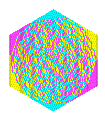
Figure 1. A random, uniformly chosen, lozenge tiling of a hexagon $\Lambda_{\epsilon}$ of diameter $\epsilon^{-1}$. As $\epsilon\to 0$, the corresponding random interface presents six “frozen regions” near the corners and a “liquid region” inside the arctic circle [10].

Such models have a family of translation-invariant Gibbs measures, with an integrable (actually determinantal) structure [22], that play the role of stationary states for the dynamics.

2. Stochastic interface growth

In a stochastic growth process, the height function $h(t)=\{h_{x}(t)\}_{x\in\mathbb{Z}^{d}}$ evolves asymmetrically, i.e. has an average non-zero drift, say positive. For instance, growth can be totally asymmetric: only moves increasing the height are allowed. It is then obvious that such Markov chain cannot have an invariant measure. One should look at interface gradients $\nabla h(t)=\{h_{x}(t)-h_{x_{0}}(t)\}_{x\in\mathbb{Z}^{d}}$ instead, where $x_{0}$ is some reference site (say the origin). Since the growth phenomenon we want to model satisfies vertical translation invariance, the transition rate at which $h_{x}$ jumps, say, to $h_{x}+1$ depends only on the interface gradients (say, the gradients around $x$) and not on the absolute height $h(t)$. Therefore, the projection of the Markov chain $h(t)$ obtained by looking at the evolution of $\nabla h(t)$ is still a Markov chain. For natural examples one expects that given a slope $\rho\in\mathbb{R}^{d}$, there exists a unique translation-invariant stationary state $\mu_{\rho}$ for the gradients, with the property that $\mu_{\rho}(h_{x+e_{i}}-h_{x})=\rho_{i},i=1,\dots,d$. A very well known example is the $(1+1)$-dimensional corner growth model: the evolution of interface gradients is just the 1-dimensional Totally Asymmetric Simple Exclusion (TASEP), whose invariant measures are iid Bernoulli product measures labelled by the particle density $\rho$. See Fig. 2.

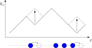
Figure 2. In the corner-growth process, heights increase by $1$, with transition rate equal to $1$, at local minima. Interpreting a negative gradient $h_{x+1}-h_{x}$ as a particle and a negative one as a hole, the dynamics of the gradients is the TASEP: particles try independently length-1 jumps to the right, with rate $1$, subject to an exclusion constraint (at most one particle per site is allowed).

If the initial height profile is sampled from $\mu_{\rho}$ (more precisely, the height gradients are sampled from $\mu_{\rho}$, while the height $h_{x_{0}}$ is assigned some arbitrary value, say zero), then on average the height increases exactly linearly with time:

(2.1) $$\mathbb{E}_{\mu_{\rho}}(h_{x}(t)-h_{x}(0))=v(\rho)t,\quad v(\rho)>0.$$

Now suppose that the initial height profile is instead close to some non-affine profile $\phi_{0}$, i.e.

(2.2) $$\epsilon h_{\epsilon^{-1}x}\stackrel{{\scriptstyle\epsilon\to 0}}{{\to}}\phi_{0}(x),\quad\forall x\in\mathbb{R}.$$

Then, one expects that, under so-called hyperbolic rescaling of space-time where $x\to\epsilon^{-1}x,t\to\epsilon^{-1}t$, one has

(2.3) $$\epsilon h_{\epsilon^{-1}x}(\epsilon^{-1}t)\stackrel{{\scriptstyle[}}{{\epsilon}}\to 0]{\mathbb{P}}{\longrightarrow}\phi(x,t)$$

where $\phi(x,t)$ is non-random and solves the first order PDE of Hamilton-Jacobi type

(2.4) $$\partial_{t}\phi(x,t)=v(\nabla\phi(x,t))$$

with $v(\cdot)$ the same function as in (2.1). A couple of remarks are important here:

• Unless $v(\cdot)$ is a linear function (which is a very uninteresting case), the PDE (2.4) develops singularities in finite time. Then, one expects $\phi(x,t)$ to solve (2.4) in the sense of vanishing viscosity.

• Viscosity solutions of (2.4) are well understood when $v(\cdot)$ is convex, since they are given by the variational Hopf-Lax formula. However, there is no fundamental reason why $v(\cdot)$ should be convex (this will be an important point in next section). Then, much less is known on the analytic side, aside from basic properties of existence and uniqueness.

• The example of the TASEP is very special in that invariant measures $\mu_{\rho}$ are explicitly known. One should keep in mind that this is an exception rather than the rule and that most examples with known stationary measures are $(1+1)$-dimensional. As a consequence, the function $v(\cdot)$ in (2.4) is in general unknown.

Next, let us consider fluctuations in the stationary process started from $\mu_{\rho}$. On heuristic grounds, one expects height fluctuations $\hat{h}_{x}(t)$ with respect to the average, linear, height profile $\mathbb{E}_{\mu_{\rho}}(h_{x}(t))=\langle\rho,x\rangle+v(\rho)t$ to be somehow described, on large space-time scales, by a stochastic PDE (KPZ equation) of the type [20]

(2.5) $$\partial_{t}\psi(x,t)=\nu\Delta\psi(x,t)+\langle\nabla\psi(x,t),H_{\rho}\nabla\psi(x,t)\rangle+\xi(x,t),$$

where:

• the Laplacian is a diffusion term that tends to locally smooth out fluctuations and $\nu>0$ is a model-dependent constant;

• the $d\times d$ symmetric matrix $H_{\rho}$ is the Hessian of the function $v(\cdot)$ computed at $\rho$ and $\langle\cdot,\cdot\rangle$ denotes scalar product in $\mathbb{R}^{d}$. This non-linear term comes just from expanding to second order the hydrodynamic PDE (2.4) around the flat solution of slope $\rho$.

• $\xi(x,t)$ is a space-time noise that models the randomness of the Markov evolution. It is well known that Eq. (2.5) is extremely singular if $\xi$ is a space-time white noise (Hairer’s theory of regularity structures [18] gives a meaning to the equation for $d=1$ but not for $d>1$). Since however we are interested in properties on large space-time scales and since lattice models have a natural “ultraviolet” space cut-off of order $1$ (the lattice spacing), we can as well imagine that the noise is not white in space and its correlation function has instead a decay length of order $1$. As a side remark, in the physics literature (e.g. [20, 45, 1]) the presence of a noise regularization in space is implicitly understood, and explicitly used in the renormalization group computations: this is the cut-off $\Lambda=1$ that appears e.g. in [1, App. B].

One should not take the above conjecture in the literal sense that the law of the space-time fluctuation process $\hat{h}_{x}(t)$ converges to the law of the solution of (2.5). Only the large-scale correlation properties of the two should be asymptotically equivalent.

For $(1+1)$-dimensional models like the TASEP and several others, a large amount of mathematical results by now supports the following picture: starting say with the deterministic condition $h_{x}(0)\equiv 0$, the standard deviation of $h_{x}(t)$ grows as $t^{\beta},\beta=1/3$, the space correlation length grows like $t^{1/z}$, where $z=3/2$ is the so-called dynamic exponent and the fluctuation field $\hat{h}_{x}(t)$ rescaled accordingly tends as $t\to\infty$ to a (non-Gaussian) limit process. We do not enter into any more detail for $(1+1)$-dimensional models of the KPZ class here, see for instance the reviews [35, 11]; let us however note that this behavior is very different from the (Gaussian) one of the stochastic heat equation with additive noise (called “Edwards-Wilkinson equation” in the physics literature), obtained by dropping the non-linear term in (2.5).

On the other hand, for $(d+1)$-dimensional models, $d\geq 3$, renormalization-group computations [20] applied to the stochastic PDE (2.5) suggest that, if the non-linear term is sufficiently small (in terms of the microscopic growth model: if the speed function $v(\cdot)$ is sufficiently close to an affine function) then non-linearity is irrelevant, meaning that the large-scale fluctuation properties of the model (or of the solution of (2.5)) are asymptotically the same as those of the stochastic heat equation: these models belong to the so-called Edwards-Wilkinson universality class. There is very recent mathematical progress in this direction: indeed, [31] states that for $d\geq 3$ the solution of (2.5) tends on large space-time scales to the solution of the Edwards-Wilkinson equation, if $H_{\rho}=\lambda\mathbb{I}$ with $\mathbb{I}$ the $d\times d$ identity matrix and $\lambda$ small enough. See also [17] where similar results are stated for the $d\geq 3$ dimensional stochastic heat equation with multiplicative noise, that is obtained from (2.5) via the Cole-Hopf transform.

The situation is richer in the borderline case of the critical dimension $d=2$, to which the next two sections are devoted.

2.1. $(2+1)$-dimensional growth: KPZ and Anisotropic KPZ (AKPZ) classes

For $(1+1)$-dimensional models, the non-linear term in (2.5) equals $v^{\prime\prime}(\rho)(\partial_{x}\psi(x,t))^{2}$: multiplying $\psi$ by a suitable constant, we can always replace $v^{\prime\prime}(\rho)\neq 0$ by a positive constant. The picture is richer for $d>1$, and in particular in the case $d=2$ we consider here. In fact, one should distinguish two cases:

1. (Isotropic) KPZ class: $\det(H_{\rho})>0$ (strictly);

2. Anisotropic KPZ (AKPZ) class: $\det(H_{\rho})\leq 0$.

According to whether a growth model has a speed function $v(\cdot)$ whose Hessian satisfies the former or latter condition, the large-scale behavior of its fluctuations is conjectured to be very different.

The isotropic KPZ class is the one considered in the original KPZ work [20]. In this case, perturbative renormalization-group arguments suggest that fluctuations of $h_{x}(t)$ (or of the solution $\psi(x,t)$ of (2.5)) grow in time like $t^{\beta}$ and that, in the stationary states, fluctuations grow in space as ${\rm Var}_{\mu_{\rho}}(h_{x}-h_{y})\sim|x-y|^{2\alpha}$, with two exponents $\beta>0,\alpha=2\beta/(\beta+1)$ that are different from those of the Edwards-Wilkinson equation: non-linearity is said to be relevant. The Edwards-Wilkinson equation can be solved explicitly and in two dimensions one finds $\alpha_{EW}=\beta_{EW}=0$ (growth in time and space is only logarithmic; the stationary state is the (log-correlated) massless Gaussian field). The values of $\alpha,\beta$ for the isotropic KPZ equation cannot be guessed by perturbative renormalization-group arguments and they are accessible only through numerical experiments (see discussion below). Note that $\alpha>0$ means that stationary height profiles are much rougher than a lattice massless Gaussian field.

The Anisotropic KPZ case was analyzed later by Wolf [45] with the same renormalization-group approach and the result came out as a surprise: non-linearity turns out to be non-relevant in this case, i.e., the growth exponents $\alpha,\beta$ are predicted to be $0$ as for the Edwards-Wilkinson equation.

Let us summarize this discussion into a conjecture:

Conjecture 2.1.

Let $v(\cdot)$ be the speed function of a (reasonable) $(2+1)$-dimensional growth model. If $\det(H_{\rho})>0$ with $H_{\rho}$ the Hessian of $v(\cdot)$ computed at $\rho$, then height fluctuations grow in time as $t^{\beta}$ for some model-independent $\beta>0$ and height fluctuations in the stationary states grow as distance to the power $2\beta/(\beta+1)$. If instead $\det(H_{\rho})\leq 0$, then $\beta=\alpha=0$ and the stationary states have the same height correlations in space as a massless Gaussian field.

Let us review the evidence in favor of this conjecture, apart from the renormalization-group argument of [20, 45] that does not provide much intuition and seems very hard to be turned into a mathematical proof:

1. A somewhat rough but suggestive argument that sheds some light on Conjecture 2.1 is given in [33, Sec. 2.2]. One imagines that in the evolution of the fluctuation field $\psi$ there are two effects. Thermal noise adds random positive or negative “bumps”, at random times, to the initially flat height profile; each bump then evolve following the hydrodynamic equation, expanded to second order:

   (2.6) $$\partial_{t}\psi=\langle\nabla\psi(x,t),H_{\rho}\nabla\psi(x,t)\rangle.$$

   It is not hard to convince oneself that, under (2.6), if both eigenvalues of $H_{\rho}$ are, say, strictly positive, then a positive bump grows larger with time and a negative bump shrinks (the reverse happens if the eigenvalues of $H_{\rho}$ are both negative). See Figure 3. On the other hand, if $\det(H_{\rho})<0$ (so that the eigenvalues of $H_{\rho}$ have opposite signs) then a positive bump spreads in the direction where the curvature of $v(\cdot)$ is positive, but its height shrinks because of the concavity of $v(\cdot)$ in the other direction (the same argument applies to negative bumps). Then, it is intuitive that when $\det(H_{\rho})<0$ height fluctuations should grow slower with time than when $\det(H_{\rho})>0$, where the effects of spreading positive bumps accumulate.

   

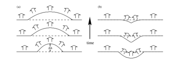
   Figure 3. Left: The time evolution of a positive bump under equation (2.6), when $\det(H_{\rho})>0$. The height $\Delta h$ of the bump is constant in time while its width grows as $t^{1/2}$. Right: a negative bump, on the other hand, develops a cusp and its height decreases as $1/t$. This figure is taken from [33].

2. There exist some growth models that satisfy a so-called “envelope property”, saying essentially that given two initial height profiles $\{h^{(j)}_{x}\}_{x\in\mathbb{Z}^{d}},j=1,2$, one can find a coupling between the corresponding profiles $\{h^{(j)}_{x}(t)\}_{x\in\mathbb{Z}^{d}}$ at time $t$ such that the evolution started from the profile $\check{h}:=\{\max(h^{(1)}_{x},h^{(2)}_{x})\}_{x\in\mathbb{Z}^{d}}$ equals $\check{h}(t)=\{\max(h^{(1)}_{x}(t),h^{(2)}_{x}(t))\}_{x\in\mathbb{Z}^{d}}$. One example is the $(2+1)$-dimensional corner-growth model analogous to that of Fig. 2 except that the interface is two-dimensional and unit cubes instead of unit squares are deposed with rate one on it. For growth models satisfying the envelope property, a super-additivity argument implies that the hydrodynamic limit (2.3) holds and moreover that the function $v(\cdot)$ in (2.4) is convex [38, 36]. While for $(2+1)$-dimensional models in this class the stationary measures $\mu_{\rho}$ and the function $v(\cdot)$ cannot be identified explicitly, convexity implies (at least in the region of slopes where $v(\cdot)$ is smooth and strictly convex) that $\det(H_{\rho})>0$: these models must belong to the isotropic KPZ class. The $(2+1)$-dimensional corner-growth model was studied numerically in [42] and it was found, in agreement with Conjecture 2.1, that $\beta\simeq 0.24$ (the numerics is sufficiently precise to rule out the value $1/4$ which was conjectured in earlier works). The same value for $\beta$ is found numerically [19] from direct simulation of (a space discretization of) the stochastic PDE (2.5) with $\det(H_{\rho})>0$.

3. For models in the AKPZ class there is no chance to get the hydrodynamic limit by simple super-additivity arguments since, as we mentioned, $v(\cdot)$ would turn out to be convex. On the other hand, as we discuss in more detail in next section, there exist some $(2+1)$-dimensional growth models for which the stationary measures $\mu_{\rho}$ can be exhibited explicitly, and they turn out to be of massless Gaussian type, with logarithmic growth of fluctuations: $\alpha=0$. For such models, one can prove also that $\beta=0$ and one can compute the speed function $v(\cdot)$. In all the known examples, a direct computation shows that $\det(H_{\rho})<0$, as it should according to Conjecture 2.1.

Remark 2.2.

Let us emphasize that, in general, it is not possible to read a priori, from the generator of the process, the convexity properties of the speed function $v(\cdot)$, and therefore its universality class. This is somehow in contrast with the situation in equilibrium statistical mechanics, where usually the universality class of a model can be guessed from symmetries of its Hamiltonian. It is even conceivable, though we are not aware of any concrete example, that there exist growth models for which the sign of $\det(H_{\rho})$ depends on $\rho$.

2.2. Mathematical results for Anisotropic KPZ growth models

As we already mentioned, there are no results other than numerical simulations or non-rigorous arguments supporting the part of Conjecture 2.1 concerning the isotropic KPZ class. Fortunately, the situation is much better for the AKPZ class, which includes several models that are to some extent “exactly solvable”.

Several of the AKPZ models for which mathematical results are available have a height function that can be associated to a two-dimensional dimer model (an exception is the Gates-Westcott model solved by Prähofer and Spohn [34]). Let us briefly recall here a few well-known facts on dimer models (we refer to [22] for an introduction). For definiteness, we will restrict our discussion to the dimer model on the infinite hexagonal graph but most of what we say about the height function and translation-invariant Gibbs states extends to periodic, two-dimensional bipartite graphs (say, $\mathbb{Z}^{2}$). A (fully packed) dimer configuration is a perfect matching of the graph, i.e., a subset $M$ of edges such that each vertex of the graph is contained in one and only one edge in $M$; as in Fig. 4, in the case of the hexagonal graph the matching can be equivalently seen as a lozenge tiling of the plane and also as a monotone discrete two-dimensional interface in three dimensional space. “Monotone” here means that the interface projects bijectively on the plane $x+y+z=0$. The height function is naturally associated to vertices of lozenges, i.e. to hexagonal faces. We will use the dimer, the tiling or the height function viewpoint interchangeably.

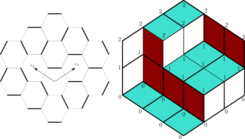
Figure 4. A perfect matching of the hexagonal lattice (left) and the corresponding lozenge tiling (right). Near each lozenge vertex is given the height of the interface w.r.t. the horizontal plane. For clarity let us emphasize that, while we draw only a finite portion of the matching/tiling, one should imagine that it extends to a matching/tiling of the infinite graph/plane.

If on the graph we choose coordinates $x=(x_{1},x_{2})$ according to the axes $e_{1},e_{2}$ drawn in Fig. 4, it is easy to see that the overall slope $\rho=(\rho_{1},\rho_{2})$ of the interface must belong to the triangle $\mathbb{T}\subset\mathbb{R}^{2}$ defined by the inequalities $0\leq\rho_{1}\leq 1,0\leq\rho_{2}\leq 1,0\leq\rho_{1}+\rho_{2}\leq 1$. It is known that, given $\rho$ in the interior of $\mathbb{T}$, there exists a unique translation-invariant ergodic Gibbs state $\pi_{\rho}$ of slope $\rho$. That is, $\pi_{\rho}$ is a (translation invariant, ergodic) probability measure on dimer configurations of the infinite graph, such that the average height slope is $\rho$ and such that, conditionally on the configuration outside any finite domain $\Lambda$, the law of the configuration inside $\Lambda$ is uniform over all dimer configurations compatible with the outside (DLR condition). In fact, much more is known: as a consequence of Kasteleyn’s theory [21], such measures have a determinantal representation. That is, the probability of a cylindrical event of the type “$k$ given edges are occupied by dimers” is given by the determinant of a $k\times k$ matrix, whose elements are the Fourier coefficients of an explicit function on the two-dimensional torus $\{(z,w)\in\mathbb{C}^{2}:|z|=|w|=1\}$ [23]. Thanks to this representation, much can be said about large-scale properties of the measures $\pi_{\rho}$. Notably, correlations decay like the inverse distance squared and the height function scales to a massless Gaussian field with logarithmic covariance structure.

Now that we have a nice candidate for a $(2+1)$-dimensional height function, we go back to the problem of defining a growth model that would hopefully be mathematically treatable and shed some light on Conjecture 2.1. To this purpose, let us remark first of all that, to a lozenge tiling as in Fig. 4, one can bijectively associate a two-dimensional system of interlaced particles. For this purpose, we will call “particles” the horizontal (or blue) lozenges (the positions of the others are uniquely determined by these) and we note that particle positions along a vertical column are interlaced with those of the two neighboring columns. See Fig. 5.

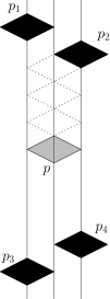
Figure 5. Each particle (or horizontal lozenge) $p$ is constrained between its four neighboring particles $p_{1},\dots p_{4}$. The three positions particle $p$ can jump to (with rate $1$) in the Borodin-Ferrari dynamics are dotted.

A first natural candidate for a growth process would be the following immediate generalization of the TASEP: each particle jumps $+1$ vertically, with rate $1$, provided the move does not violate the interlacement constraints. Actually, this is nothing but the three-dimensional corner-growth model. As we already mentioned, this should belong to the isotropic KPZ class and its stationary measures $\mu_{\rho}$ should be extremely different from the Gibbs measures $\pi_{\rho}$, with a power-like instead of logarithmic growth of fluctuations in space. Unfortunately, none of this could be mathematically proved so far.

In the work [4], A. Borodin and P. Ferrari considered instead another totally asymmetric growth model where each particle can jump an unbounded distance $n$ upwards, with rate independent of $n$ (say, rate $1$), provided the interlacements are still satisfied after the move. See Fig. 5. The situation is then entirely different with respect to the corner-growth process: the two processes belong to two different universality classes. If the initial condition of the process is a suitably chosen, deterministic, fully packed particle arrangement (see Fig. 1.1 in [4]), it was shown that the height profile rescaled as in (2.3) does converge to a deterministic limit $\phi(\cdot,t)$, that solves the Hamilton-Jacobi equation (2.4) with

(2.7) $$v(\rho)=\frac{1}{\pi}\frac{\sin(\pi\rho_{1})\sin(\pi\rho_{2})}{\sin(\pi(\rho_{1}+\rho_{2}))}.$$

A couple of remarks are important for the subsequent discussion:

• with the initial condition chosen in [4], $\phi(x,t)$ turns out to be a classical solution of (2.4). That is, the characteristic lines of the PDE do not cross at positive times (we emphasize that this is due to the specific form of the chosen initial profile and not to the form of $v(\cdot)$).

• An explicit computation shows that $\det(H_{\rho})<0$ for the function (2.7): this growth model is then a candidate to belong to the AKPZ class.

As mentioned in Remark 2.2 above, let us emphasize that we see no obvious way to guess a priori that the corner growth process and the “long-jump” one should belong to different universality classes.

Various other results were proven in [4], but let us mention only two of them, that support the conjecture that this model indeed belongs to the AKPZ class:

1. the fluctuations of $h_{\epsilon^{-1}x}(\epsilon^{-1}t)$ around its average value are of order $\sqrt{\log 1/\epsilon}$ (the growth exponent is $\beta=0$) and, once rescaled by this factor, they tend to a Gaussian random variable;

2. the local law of the interface gradients at time $\epsilon^{-1}t$ around the point $\epsilon^{-1}x$ tends to the Gibbs measure $\pi_{\rho}$ with $\rho=\nabla\phi(x,t)$.

Remark 2.3.

The basic fact behind the results of [4] is that for the specific choice of initial condition, one can write [4, Th. 1.1] the probability of certain events of the type “there is a particle at position $x_{i}$ at time $t_{i},i\leq k$” as a $k\times k$ determinant, to which asymptotic analysis can be applied. The same determinantal properties hold for other “integrable” initial conditions, but they are not at all a generic fact.

Point (2) above clearly suggests that the Gibbs measures $\pi_{\rho}$ should be stationary states for the interface gradients. In fact, this is a result I later proved:

Theorem 2.4.

[43, Th. 2.4] For every slope $\rho$ in the interior of $\mathbb{T}$, the measure $\pi_{\rho}$ is stationary for the process of the interface gradients.

Recall that, as discussed above, the Gibbs measures $\pi_{\rho}$ of the dimer model have the large-scale correlation structure of a massless Gaussian field and indeed Conjecture 2.1 predicts that stationary states of AKPZ growth processes behave like massless fields. Most of the technical work in [43] is related to the fact that, since particles can perform arbitrarily long jumps with a rate that does not decay with the jump length, it is not clear a priori that the process exists at all: one can exhibit initial configurations such that particles jump to $+\infty$ in finite time (this issue does not arise in the work [4] where, thanks to the chosen initial condition, there is no difficulty in defining the infinite-volume process). In [43] it is shown via a comparison with the one-dimensional Hammersley process [39] that, for a typical initial condition sampled from $\pi_{\rho}$, particles jump almost surely a finite distance in finite time and that, despite the unbounded jumps, perturbations do not spread instantaneously through the system. This means that if two initial configurations differ only on a subset $S$ of the lattice, their evolutions can be coupled so that at finite time $t$ they are with high probability equal sufficiently far away from $S$ (how far, depending on $t$).

To follow the general program outlined above, once the stationary states are known, one would like to understand the growth exponent $\beta$ for the stationary process. We proved the following, implying $\beta=0$:

Theorem 2.5.

[43, Th. 3.1] For every lattice site $x$, we have

(2.8) $$\limsup_{t\to\infty}\mathbb{P}_{\pi_{\rho}}\left(|h_{x}(t)-\mathbb{E}_{\pi_{\rho}}(h_{x}(t))|\geq u\sqrt{\log t}\right)\stackrel{{\scriptstyle u\to\infty}}{{\longrightarrow}}0$$

where

(2.9) $$\mathbb{E}_{\pi_{\rho}}(h_{x}(t))=v(\rho)t+\langle x,\rho\rangle.$$

To be precise:

• in the statement of [43, Th. 3.1] there is a technical restriction on the slope $\rho$, that was later removed in joint work with S. Chhita and P. Ferrari [9];

• the proof that the speed of growth $v(\cdot)$ in (2.9) is the same as the function $v(\cdot)$ in (2.7), as it should, was obtained by S. Chhita and P. Ferrari in [8] and requires a nice combinatorial property of the Gibbs measures $\pi_{\rho}$.

With reference to Remark 2.3 above, it is important to emphasize that there is no known determinantal form for the space-time correlations of the stationary process; for the proof of (2.8) we used a more direct and probabilistic method.

Finally, it is natural to try to obtain a hydrodynamic limit for the height profile. Recall that in [4] such a result was proven for an “integrable” initial condition that allowed to write certain space-time correlations, and as a consequence the average particle currents, in determinantal form. On the other hand, convergence to the hydrodynamic limit should be a very robust fact and not rely on such special structure. We have indeed:

Theorem 2.6.

[29, Th. 3.5 and 3.6] Let the initial height profile satisfy (2.2), with $\phi_{0}$ a Lipshitz function with gradient in the interior of $\mathbb{T}$. Let one of the following two conditions be satisfied:

• $\phi_{0}$ is $C^{2}$ and the time $t$ is smaller than $T$, the maximal time up to which a classical solution of (2.4) exists;

• $\phi_{0}$ is either convex or concave (in which case we put no restriction on $t$).

Then, the convergence (2.3) holds, with $\phi(x,t)$ the viscosity solution of (2.4).

The restriction to either small times or to convex/concave profile is due to the fact that we have in general little analytic control on the singularities of (2.4), due to the non-convexity of $v(\cdot)$. For convex initial profile, the viscosity solution of the PDE is given by a Hopf variational form and this allows to bypass these analytic difficulties. Let us emphasize, to avoid any confusion, that even in the case of convex initial profile the solution does in general develop singularities (shocks), i.e. discontinuities in space of the gradient $\nabla\phi(x,t)$.

Open problem 2.7.

Are height fluctuations still $O(\sqrt{\log t})$ at the location of shocks?

Another important observation is the following. Given that we know explicitly the stationary states of the process and that the dynamics is monotone (i.e, if an initial profile is higher than another, under a suitable coupling it will stay higher as time goes on), it is tempting to try to apply the method developed by Rezakhanlou in [37], that gives under such circumstances convergence of the height profile of a growth model to the viscosity solution of the limit PDE. The delicate point is however that [37] crucially requires that perturbations spread at finite speed through the system, so that one can analyze the evolution “locally”, in small enough windows where the profile can be approximated by one sampled from $\mu_{\rho}$, with suitably chosen slope $\rho$ that depends on the window location. Due to unboundedness of particle jumps, however, the “finite-speed propagation property” might fail in our case and in any case it cannot hold uniformly for all initial conditions. Most of the technical work in [29] is indeed devoted to proving that one can localize the dynamics despite the long jumps. A crucial fact is that we show that the growth process under consideration can be reformulated through a so-called Harris-like graphical construction.

2.2.1. Extensions and open problems

There are various ways how the “lozenge tiling dynamics with long particle jumps” of previous section can be generalized to provide other $(2+1)$-dimensional growth processes in the AKPZ class. One such generalization was given in [43, Sec. 3.1]. There, one starts with the observation that: (i) as was the case for lozenge tilings, also domino tilings of $\mathbb{Z}^{2}$ (dominoes being $2\times 1$ rectangles, horizontal or vertical, see Fig. 6) have a natural height function interpretation, and (ii) a domino tiling can be bijectively mapped to a two-dimensional system of interlaced particles (interlacement constraints are different than in lozenge case).

Figure 6. A perfect matching of the square lattice and the corresponding domino tiling (dotted). See [9, Fig. 2] for the definition of “particles” and their interlacing relations, and [22] for the definition of the height function.

This suggests a growth process where particles jump in an asymmetric fashion and the transition rate is independent of the jump length, jumps being limited only by the interlacement constraints. Then, the same results that were proven for the lozenge dynamics (notably, stationarity of the Gibbs measures, logarithmic correlations in space in the stationary states ($\alpha=0$) and logarithmic growth of fluctuations in the stationary process implying $\beta=0$) hold in this case too. The speed of growth $v(\cdot)$ for the domino dynamics was later computed in a joint work with S. Chhita and P. Ferrari [9, Th. 2.3]: it turns out to be rather more complicated than (2.7), but it is still an explicit function for which one can prove with some effort that the Hessian has negative determinant, in agreement with Conjecture 2.1.

Finally, there is yet another class of driven two-dimensional interlaced particle systems, that was introduced in [2]. While these have rather a group-theoretic motivation, these processes can also be viewed as $(2+1)$-dimensional growth models and actually the main result of [2] can be seen as a hydrodynamic limit for the height function [2, Sec. 3.3]. Once again, direct inspection of the Hessian of the velocity function shows that these models belong to the AKPZ class, so these provide other natural candidates where Wolf’s prediction of logarithmic growth of fluctuations can be tested (the logarithmic nature of fluctuation correlations is conjectured in [2]; we are not aware of an actual proof).

In conclusion, there are now quite a few $(2+1)$-dimensional growth models in the AKPZ class for which Wolf’s predictions in Conjecture 2.1 can be verified. There is however one aspect one may find rather unsatisfactory. Both for the lozenge tiling dynamics, where the speed function turns out to be given by (2.7) and for its domino tiling generalization, where $v(\cdot)$ is a much more complicated-looking combination of ratios of trigonometric functions (see [9, Eq. (2.6)]) and also for the interlaced particle dynamics of [2], one verifies via brute-force computation that the Hessian of $H_{\rho}$ of the corresponding velocity function $v(\cdot)$ has negative determinant. The frustrating fact is that via the explicit computation one does not see at all how the sign of the determinant the Hessian is related to the model being in the Edwards-Wilkinson universality class! We are still far from having a meta-theorem saying “if the exponents $\alpha$ and $\beta$ are zero, then the determinant of the Hessian is negative”. Up to now, we have essentially heuristic arguments and “empirical evidence” based on a few mathematically treatable models.

Open problem 2.8.

It would be very interesting to prove that the Hessian of the velocity function for the growth models just mentioned has negative determinant without going through the explicit computation of the second derivatives.

2.2.2. Slow decorrelation along the characteristics

The results we discussed in Sections 2.2 and 2.2.1 (growth of fluctuation variance with time and spatial correlations in the stationary state) concern fluctuation properties at a single time. Another question of great interest is how fluctuations at different space-time points $(x_{i},t_{i})$ are correlated. For $(1+1)$-dimensional growth models in the KPZ class, the following picture has emerged [12]: correlation decay slowly along the characteristic lines of the PDE (2.4), and faster along any other direction. For instance, take two space-time points $(x_{1},t_{1})$ and $(x_{2},t_{2}),t_{1}<t_{2}$ and think of $t_{2}$ large. If the two points are on the same characteristic line, then the height fluctuations (divided by the rescaling factor $t_{i}^{\beta}=t_{i}^{1/3}$) will be almost perfectly correlated as long as $t_{2}-t_{1}\ll t_{2}$. If instead the two points are not along a characteristic line, then correlation will be essentially zero as soon as $t_{2}-t_{1}\gg t_{2}^{1/z},z=3/2$.

It has been conjectured [12, 4] that a similar phenomenon of slow decorrelation along the characteristic lines should occur for $(2+1)$-dimensional growth. For the AKPZ models described in the previous sections, it is still an open problem to prove anything in this direction. In the work [3] in collaboration with A. Borodin and I. Corwin, we studied a growth model that depends on a parameter $q\in[0,1)$: for $q=0$ it reduces to the long-jump lozenge dynamics of [4, 43], while if $q\to 1$ and particle distances are suitably rescaled the dynamics simplifies in that fluctuations become Gaussian. In this limit, we were able to prove that, if height fluctuations are computed along characteristic lines, their correlations converge to those of the Edwards-Wilkinson equation and in particular they are large as long as $t_{2}-t_{1}\ll t_{2}$. If correlations are computed instead along a different direction, then they are essentially zero as soon as $t_{2}-t_{1}\gg t_{2}^{1/z}$, where $z=2$ is the dynamic exponent of the Edwards-Wilkinson equation.

3. Interface dynamics at thermal equilibrium

Let us now move to reversible interface dynamics (we refer to [41, 15] for an introduction). We can imagine that the interface is defined on a finite subset $\Lambda_{\epsilon}$ of $\mathbb{Z}^{d}$ of diameter $O(\epsilon^{-1})$, say the cubic box $[0,\dots,\epsilon^{-1}]^{d}$ so that after the rescaling $x=\epsilon^{-1}\xi$, the space coordinate $\xi$ is in the unit cube. We impose Dirichlet boundary conditions, i.e., for $x\in\partial\Lambda_{\epsilon}$ the height $h_{x}(t)$ is fixed to some time-independent value $\bar{h}_{x}$. The way to model the evolution of a phase boundary at thermal equilibrium is to take a Markov process with stationary and reversible measure of the Boltzmann-Gibbs form (we absorb the inverse temperature into the potential $V$)

(3.1) $$\pi_{\Lambda_{\epsilon}}(h)\propto e^{-1/2\sum_{x\sim y}V(h_{x}-h_{y})}$$

where the sum runs, say, on nearest neighboring pairs of vertices. Note that the potential $V$ depends only on interface gradients and not on the absolute height itself: this reflects the vertical translation invariance of the problem (apart from boundary condition effects). A minimal requirement on $V$ is that it diverges to $+\infty$ when $|h_{x}-h_{y}|\to\infty$: the potential has the effect of “flattening” the interface and suppressing wild fluctuations, in agreement with the observed macroscopic flatness of phase boundaries. (Much more stringent conditions have to be imposed on $V$ to actually prove any result.) Note also that the measure $\pi_{\Lambda_{\epsilon}}$ depends on the boundary height $\bar{h}_{\cdot}$: if $\bar{h}_{\cdot}$ is fixed so that the average slope is $\rho\in\mathbb{R}^{d}$, i.e. $\pi_{\Lambda_{\epsilon}}(h_{x}-h_{x+e_{i}})=\rho_{i},i\leq d$, then we write $\pi_{\Lambda_{\epsilon},\rho}$.

There are various choices of Markov dynamics that admit (3.1) as stationary reversible measure. A popular choice is the heat-bath or Glauber dynamics: with rate $1$, independently, each height $h_{x}(t)$ is refreshed and the new value is chosen from the stationary measure $\pi_{\Lambda_{\epsilon}}$ conditioned on the values of $h_{y}(t)$ with $y$ ranging over the nearest neighbors of $x$. Another natural choice, when the heights are in $\mathbb{R}$ rather than in $\mathbb{Z}$, is a Langevin-type dynamics where each $h_{x}(t)$ is subject to an independent Brownian noise, plus a drift that depends on the height differences between $x$ and its neighboring sites, chosen so that (3.1) is reversible.

As we mentioned, under reasonable assumptions, a diffusive hydrodynamic limit is expected:

(3.2) $$\epsilon h_{\epsilon^{-1}x}(\epsilon^{-2}t)\stackrel{{\scriptstyle[}}{{\epsilon}}\to 0]{\mathbb{P}}{\longrightarrow}\phi(x,t)$$

where $\phi$ is deterministic. Due to the diffusive scaling of time, the PDE solved by $\phi$ will be of second order and in general non-linear:

(3.3) $$\partial_{t}\phi(x,t)=\mu(\nabla\phi(x,t))\sum_{i,j=1}^{d}\sigma_{i,j}(\nabla\phi(x,t))\frac{\partial^{2}}{\partial_{x_{i}}\partial_{x_{j}}}\phi(x,t).$$

The factors $\mu$ and $\sigma_{i,j}$ have a very different origin, which is why we have not written the equation in terms of the combination $\tilde{\sigma}_{i,j}:=\mu\sigma_{i,j}$ instead. The slope-dependent prefactor $\mu>0$ is called mobility and will be discussed in a moment. As for $\sigma_{i,j}$, let the convex function $\sigma:\rho\in\mathbb{R}^{d}\mapsto\sigma(\rho)\in\mathbb{R}$ denote the surface tension of the model at slope $\rho$ [15], i.e. minus the limit as $\epsilon\to 0$ of $1/{|\Lambda_{\epsilon}|}$ times the logarithm of the normalization constant of the probability measure (3.1) when $\pi_{\Lambda_{\epsilon}}=\pi_{\Lambda_{\epsilon,\rho}}$. Then, $\sigma_{i,j}$ denotes the second derivative of $\sigma$ w.r.t. the $i^{th}$ and $j^{th}$ argument. Convexity of $\sigma$ implies that the matrix $\{\sigma_{i,j}(\nabla\phi)\}_{i,j=1,\dots,d}$ is positive definite, so the PDE (3.3) is of parabolic type. We emphasize that the surface tension, hence $\sigma_{i,j}$, are defined purely in terms of the stationary measure (3.1). All the dependence on the Markov dynamics is in the mobility $\mu$. Remark also that one can rewrite (3.3) in the following more evocative form:

(3.4) $$\partial_{t}\phi(x,t)=-\mu(\nabla\phi(x,t))\frac{\delta F[\phi(\cdot,t)]}{\delta\phi(x,t)}$$

where $F[\phi(\cdot)]=\int dx\,\sigma(\nabla\phi)$ is the surface tension functional and $\delta F/\delta\phi$ denotes its first variation. In other words, the hydrodynamic equation is nothing but the gradient flow w.r.t. the surface tension functional, modulated by a slope-dependent mobility prefactor.

Via linear response theory one can guess a Green-Kubo-type expression for the mobility [41]. This turns out to be given as (say that the heights $h_{x}$ are discrete, so that the dynamics is a Markov jump process; the formula is analogous for Langevin-type dynamics)

(3.5) $$\mu(\rho) = \lim_{\epsilon\to 0}\frac{1}{2|\Lambda_{\epsilon}|}\pi_{\Lambda_{\epsilon},\rho}\left[\sum_{x\in\Lambda_{\epsilon}}\sum_{n}c_{x}^{n}(h)n^{2}\right]$$

(3.6) $$- \int_{0}^{\infty}dt\lim_{\epsilon\to 0}\frac{1}{|\Lambda_{\epsilon}|}\sum_{x,x^{\prime}\in\Lambda_{\epsilon}}\sum_{n,n^{\prime}}\mathbb{E}_{\pi_{\Lambda_{\epsilon},\rho}}\left[c_{x}^{n}(h(0))n\;c_{x^{\prime}}^{n^{\prime}}(h(t))n^{\prime}\right]$$

where $c_{x}^{n}(h)$ is the rate at which the height at $x$ increases by $n\in\mathbb{Z}$ in configuration $h$, $\mathbb{E}_{\pi_{\Lambda_{\epsilon},\rho}}$ denotes expectation w.r.t. the stationary process started from $\pi_{\Lambda_{\epsilon},\rho}$ and $h(t)$ denotes the configuration at time $t$. Note that the first term involves only equilibrium correlation functions in the infinite volume stationary measure $\pi_{\rho}=\lim_{\Lambda\to\mathbb{Z}^{d}}\pi_{\Lambda_{\epsilon},\rho}$. The same is not true for the second one, which involves a time integral of correlations at different times for the stationary process. These are usually not explicitly computable even when $\pi_{\rho}$ is known. It may however happen for certain models that, by a discrete summation by parts w.r.t. the $x$ variable, $\sum_{x}\sum_{n}c_{x}^{n}(h)$ is deterministically zero, for any configuration $h$: one says then that a gradient condition is satisfied (a classical example is symmetric simple exclusion). In this case (3.6) identically vanishes and one is in a much better position to prove convergence to the hydrodynamic equation.

For the “Ginzburg-Landau (GL)” model [41] where heights $h_{x}$ are continuous variables and the dynamics is of Langevin type, if the potential $V(\cdot)$ is convex and symmetric then, in any dimension $d$, the gradient condition is satisfied and moreover the remaining average in the Green-Kubo formula is immediately computed, leading to a constant mobility: $\mu(\rho)=1$. In this situation, Funaki and Spohn [16] proved convergence of the height profile to (the weak solution of) (3.3) for the GL model, for any $d\geq 1$. (They look at weak solutions because for $d>1$ it is not known whether the surface tension of the GL model is $C^{2}$ and the coefficients $\sigma_{i,j}$ are well defined and smooth). Until recently, to my knowledge, there was no other known interface model in dimension $d>1$ where mathematical results of this type were available.

Before presenting our recent results for $(2+1)$-dimensional interface dynamics let us make two important observations:

• Not only for most natural interface dynamics in dimension $d>1$ one is unable to prove a hydrodynamic convergence of the type (3.2): the situation is actually much worse. As (3.2) suggests, the correct time-scale for the system to reach stationarity (measured either by $T_{rel}:=1/{\rm gap}(\mathcal{L})$, with gap$(\mathcal{L})$ denoting the spectral gap of the generator, or by the so-called total variation mixing time $T_{mix}$) should be of order $\epsilon^{-2}$ (logarithmic corrections are to be expected for the mixing time). On the other hand, for most natural models it not even proven that such characteristic times are upper bounded by a polynomial of $\epsilon^{-1}$! For instance, for the well-known $(2+1)$-dimensional SOS model at low temperature, the best known upper bound for $T_{rel}$ and $T_{mix}$ is a rather poor $O(\exp(\epsilon^{-1/2+o(1)}))$ [6, Th. 3].

• In dimension $d=1$, natural Markov dynamics of discrete interfaces are provided by conservative lattice gases on $\mathbb{Z}$ (e.g. symmetric exclusion processes or zero-range processes), just by interpreting the number of particles at site $x$ as the interface gradient $h_{x}-h_{x-1}$ at $x$. Similarly, conservative continuous spin models on $\mathbb{Z}$ translate into Markov dynamics for one-dimensional interface models with continuous heights. Then, a hydrodynamic limit for the height function follows from that for the particle density (see e.g. [24, Ch. 4 and 5] for the symmetric simple exclusion and for a class of zero-range processes, and for instance [13] for the $d=1$ Ginzburg-Landau model). For $d>1$, instead, there is in general no obvious way of associating a height function to a particle system on $\mathbb{Z}^{d}$. Also, for $d=1$ there are robust methods to prove that the inverse spectral gap is $T_{rel}=O(\epsilon^{-2})$, see e.g. [24, 5].

3.1. Reversible tiling dynamics, mixing time and hydrodynamic equation

In this section, I briefly review a series of results obtained in recent years in collaboration with Pietro Caputo, Benoît Laslier and Fabio Martinelli. In these works we study $(2+1)$-dimensional interface dynamics where the height function $\{h_{x}\}_{x\in\Lambda_{\epsilon}}$ is discrete and is given by the height function of a tiling model, either by lozenges or by dominoes, as explained in Section 2.2. In contrast with the $(2+1)$-dimensional Anisotropic KPZ growth models described in Section 2.2, that are also Markov dynamics of tiling models, here we want a reversible process because we wish to model interface evolution at thermal equilibrium. A natural candidate is the “Glauber” dynamics obtained by giving rate $1$ to the elementary rotations of tiles around faces of the graph, see Fig. 7 for the case of lozenge tilings.

Figure 7. The elementary updates for the Glauber dynamics of the lozenge tiling model correspond to the rotation of three lozenges (equivalently, three dimers) around a hexagonal face. The transition rate is $1$ both for the update and the reverse one. Note that in the three-dimensional corner growth model only the forward transition would be allowed.

In terms of the height function, elementary moves correspond to changing the height by $\pm 1$ at single sites. Since all elementary rotations have the same rate, the uniform measure over the finitely many tiling configurations in $\Lambda_{\epsilon}$ is reversible. As a side remark, this measure can be written in the Boltzmann-Gibbs form (3.1) with a potential $V$ taking values $0$ or $+\infty$. Let us also remark that, as discussed in [7], this dynamics is equivalent to the zero-temperature Glauber dynamics of the three-dimensional Ising model with Dobrushin boundary conditions.

In agreement with the discussion of the previous section, if the tiled region is a reasonably-shaped domain $\Lambda_{\epsilon}$ of diameter $O(\epsilon^{-1})$, one expects $T_{rel}$ and $T_{mix}$ to be $\approx\epsilon^{-2}$ and the height profile to converge under diffusive rescaling to the solution of a parabolic PDE. Until recently, however, all what was known rigorously was that $T_{rel}$ and $T_{mix}$ are upper bounded as $O(\epsilon^{-n})$ for some finite $n>2$!

Open problem 3.1.

This polynomial upper bound was proven in [30] for the Glauber dynamics on either lozenge or domino tiling (the same proof works for tilings associated to the dimer model on certain graphs with both hexagonal and square faces, as shown in [25]). The method does not seem to work, however, for general planar bipartite graphs. For instance, a polynomial upper bound for $T_{rel}$ or $T_{mix}$ of the Glauber dynamics of the dimer model on the square-octagon graph (see Fig. 9 in [22]) is still unproven.

Under suitable conditions, we improved this $O(\epsilon^{-n})$ upper bound into an almost optimal one:

Theorem 3.2 (Informal statement).

If the boundary height on $\partial\Lambda_{\epsilon}$ is such that the average height under the measure $\pi_{\Lambda_{\epsilon}}$ tends to an affine function as $\epsilon\to 0$, then $T_{mix}$ and $T_{rel}$ are $O(\epsilon^{-2+o(1)})$ [7, 25].

Later [26], we proved a result in the same spirit under the sole assumption that the limit average height profile is smooth and in particular has no “frozen regions” [22].

Let us emphasize that there are very natural domains $\Lambda_{\epsilon}$ such that the average equilibrium height profile in the $\epsilon\to 0$ limit does have “frozen regions”:

Open problem 3.3.

Let $\Lambda_{\epsilon}$ be the hexagonal domain of side $\epsilon^{-1}$, see Fig. 1. Prove that, for the lozenge tiling Glauber dynamics, $T_{rel}$ and/or $T_{mix}$ are $O(\epsilon^{-2+o(1)})$. The best upper bound that can be extracted from [44] plus the so-called Peres-Winkler censoring inequalities [32] is $O(\epsilon^{-4+o(1)})$.

The proofs of the previously known polynomial upper bounds on the mixing time were based on smart and rather simple path coupling arguments [30]. To get our almost optimal bounds [7, 25, 26], there are at least two new inputs:

• our proof consists in a comparison between the actual interface dynamics and an auxiliary one that evolves on almost-diffusive time-scales $\approx\epsilon^{-2+o(1)}$ and that essentially follows the conjectural hydrodynamic motion where interface drift is proportional to its curvature;

• to control the auxiliary process, we crucially need very refined estimates on height fluctuation for the equilibrium measure $\pi_{\Lambda_{\ell}}$ on domains of mesoscopic size $\ell=\epsilon^{-a},1/2\leq a\leq 1$, with various types of boundary conditions.

For the Glauber dynamics with elementary moves as in Fig. 7, it seems hopeless to prove a hydrodynamic limit on the diffusive scale. In particular, no form of “gradient condition” is satisfied. Fortunately, there exists a more friendly variant of the Glauber dynamics, introduced in [30], where a single update consists in “tower moves” changing the height by the same amount $\pm 1$ at $n\geq 0$ aligned sites, as in Fig. 8.

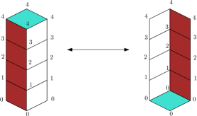
Figure 8. A “tower move” transition with $n=4$ and the reverse transition. The transition rates equal $1/n=1/4$. Note that the height decreases by $1$ at four points.

The integer $n$ is not fixed here, in fact transitions with any $n$ are allowed but the transition rate decreases with $n$ and actually it is taken to equal to $1/n$. It is immediate to verify that this dynamics is still reversible w.r.t. the uniform measure. For this modified dynamics, together with B. Laslier we realized in [27] that a microscopic summation by parts implies that the term (3.6) in the definition of the mobility vanishes, and actually we could explicitly compute $\mu$, that turns out to be non-trivial and non-linear:

(3.7) $$\mu(\rho)=\frac{1}{\pi}\frac{\sin(\pi\rho_{1})\sin(\pi\rho_{2})}{\sin(\pi(\rho_{1}+\rho_{2}))}.$$

Recall that, in contrast, the mobility of the Ginzburg-Landau model is slope-independent [41]. Later, in [28, Th. 2.7], we could turn our arguments into a full proof of convergence of the height profile to the solution of the PDE:

Theorem 3.4 (Informal statement).

If the initial profile $\phi_{0}$ is sufficiently smooth, one has for every $t>0$

(3.8) $$\lim_{\epsilon\to 0}\frac{1}{|\Lambda_{\epsilon}|}\sum_{x\in\Lambda_{\epsilon}}\mathbb{E}\left|\epsilon h_{x}(\epsilon^{-2}t)-\phi(\epsilon x,t)\right|^{2}=0,$$

with $\phi(x,t)$ the solution of (3.3)

(For technical reasons, we had to work with periodic instead of Dirichlet boundary conditions). A couple of comments are in order:

• As the reader may have noticed, the function (3.7) is exactly the same as the “speed function” $v(\rho)$ of the growth model discussed in Section 2.2, see formula (2.7). This is not a mere coincidence. Actually, one may see this equality as an instance of the so-called Einstein relation between diffusion and conductivity coefficients [40].

• We mentioned earlier that convergence of the height profile of the Ginzburg-Landau model to the limit PDE has been proved [16] only in a weak sense. In our case, instead, we have strong convergence to classical solutions of (3.3) that exist globally because the coefficients $\mu(\cdot),\sigma_{i,j}(\cdot)$ turn out to be smooth functions of the slope.

• A fact that plays a crucial role in the proof of the hydrodynamic limit is that the PDE (3.3) contracts the $L^{2}$ distance $D_{2}(t)=\int dx(\phi^{(1)}(x,t)-\phi^{(2)}(x,t))^{2}$ between solutions. I believe this is not a trivial or general fact: in fact, to prove contraction [28], we use the specific form (3.7) of $\mu$ and the explicit expression of $\sigma_{i,j}$ for the dimer model. (Note that if the mobility were constant, as it is for the Ginzburg-Landau model, $L^{2}$ contraction would just be a consequence of convexity of the surface tension $\sigma$). I think it is an intriguing question to understand whether the identities (see [28, Eqs. (6.19)-(6.22)]) leading to $dD_{2}(t)/dt\leq 0$ have any thermodynamic interpretation.

To conclude this review, let us mention that new dynamical phenomena, taking place on time-scales much longer than diffusive, can occur at low temperature, for interface models undergoing a so-called “roughening transition”. That is, up to now we considered situations where the equilibrium Gibbs measure for the interface in a $\epsilon^{-1}\times\epsilon^{-1}$ box $\Lambda_{\epsilon}$ scales to a massless Gaussian field as $\epsilon\to 0$ and in particular ${\rm Var}_{\pi_{\Lambda_{\epsilon}}}(h_{x})\approx\log(1/\epsilon)$ if $x$ is, say, the center of the box. The interface is said to be “rough” in this case, because fluctuations diverge as $\epsilon\to 0$. For some interface models, notably the well-known Solid-on-Solid (SOS) model where the potential $V$ in (3.1) equals $T^{-1}|h_{x}-h_{y}|$ and heights are integer-valued and fixed to $0$ around the boundary, it is known that at low enough temperature $T$ the interface is instead rigid, with $\limsup_{\epsilon\to 0}{\rm Var}_{\pi_{\Lambda_{\epsilon}}}(h_{x})<\infty$, while the variance grows logarithmically at high temperature [14]. The temperature $T_{r}$ separating these two regimes is called “roughening temperature”.

In a work with P. Caputo, E. Lubetzky, F. Martinelli and A. Sly [6] we discovered that rigidity of the interface can produce a dramatic slowdown of the dynamics, if the interface is constrained to stay above a fixed level, say level $0$:

Theorem 3.5.

[6] Consider the Glauber dynamics for the $(2+1)$-dimensional SOS model at low enough temperature, with $0$ boundary conditions on $\partial\Lambda_{\epsilon}$ and with the positivity constraint $h_{x}\geq 0$ for every $x\in\Lambda_{\epsilon}$. Then, the relaxation and mixing times satisfy

(3.9) $$T_{mix}\geq T_{rel}\geq c\exp[{c\;\epsilon^{-1}}]$$

for some positive, temperature-dependent constant $c$.

What we actually prove is that there is a cascade of metastable transitions, occurring on all time-scales $\exp({\epsilon^{-a}})$, $a<0\leq 1$. Strange as this may look, these results do not exclude that a hydrodynamic limit on the diffusive scale, as in (3.2)-(3.3), might occur. That is, the rescaled height profile $\epsilon h_{\epsilon^{-1}x}(\epsilon^{-2}t)$ could follow an equation like (3.3), so that at times $\gg\epsilon^{-2}$ the profile would be macroscopically zero (because $\phi\equiv 0$ is the equilibrium point of the PDE (3.3) with zero boundary conditions) but smaller-scale height fluctuations would need enormously more time, of the order $T_{mix}\approx\exp(\epsilon^{-1})$, to relax to equilibrium.

We are light years away from being able to actually prove a hydrodynamic limit for the $(2+1)$-dimensional SOS model. The following open problem is given just to show how little we know in this respect:

Open problem 3.6.

Take the Glauber dynamics for the $(2+1)$-d SOS model at low temperature, with initial condition $\epsilon\,h_{x}=1$ for every $x\in\Lambda_{\epsilon}$. Is it true that, for some $N<\infty$, at time $t=1/\epsilon^{N}$ all rescaled heights $\epsilon\,h_{x}(t)$ are with high probability lower than, say, $1/2$ (which is much larger than $\epsilon\log\epsilon^{-1}$, that is the typical value under the equilibrium measure of $\max_{x\in\Lambda_{\epsilon}}[\epsilon\,h_{x}]$)?

Acknowledgements

This work was partially funded by the ANR-15-CE40-0020-03 Grant LSD, by the CNRS PICS grant “Interfaces aléatoires discrètes et dynamiques de Glauber” and by MIT-France Seed Fund “Two-dimensional Interface Growth and Anisotropic KPZ Equation”.

References

- [1] A.-L. Barabási and H. E. Stanley, Fractal concepts in surface growth, Cambridge University Press, 1995.
- [2] A. Borodin, A. Bufetov and G. Olshanski, Limit shapes for growing extreme characters of , Ann. Appl. Probab. 25 (2015), 2339-2381.
- [3] A. Borodin, I. Corwin, F. L. Toninelli, Stochastic heat equation limit of a d growth model, Comm. Math. Phys. 350 (2017), 957-984
- [4] A. Borodin and P.L. Ferrari, Anisotropic Growth of Random Surfaces in Dimensions, Comm. Math. Phys., 325 (2014), 603–684.
- [5] P. Caputo, Spectral gap inequalities in product spaces with conservation laws, Adv. Studies Pure Math. 39 (2004), 53-88.
- [6] P. Caputo, E. Lubetzky, F. Martinelli, A. Sly, F. L. Toninelli, Dynamics of 2+1 dimensional SOS surfaces above a wall: slow mixing induced by entropic repulsion, Ann. Probab. 42 (2014), 1516-1589
- [7] P. Caputo, F. Martinelli, F.L. Toninelli, Mixing times of monotone surfaces and SOS interfaces: a mean curvature approach, Comm. Math. Phys. 311 (2012), 157–189.
- [8] S. Chhita and P.L. Ferrari, A combinatorial identity for the speed of growth in an anisotropic KPZ model, to appear on Ann. Inst. H. Poincaré D, arXiv:1508.01665, 2015.
- [9] S. Chhita, P. L. Ferrari, F. L. Toninelli, Speed and fluctuations for some driven dimer models, arXiv:1705.07641
- [10] H. Cohn, M. Larsen, J. Propp, The Shape of a Typical Boxed Plane Partition, New York J. Math. 4 (1998), 137-165
- [11] I. Corwin, The Kardar-Parisi-Zhang equation and universality class, Random matrices: Theory and applications, 1(01) (2012), 1130001.
- [12] P. L. Ferrari, Slow decorrelations in KPZ growth, J. Stat. Mech. (2008), P07022
- [13] J. Fritz, On the Hydrodynamic Limit of a Ginzburg Landau Lattice Model , Prob. Theory Rel. Fields 81 (1989), 291-318.
- [14] J. Fröhlich, and T. Spencer, The Kosterlitz–Thouless transition in two-dimensional abelian spin systems and the Coulomb gas, Comm. Math. Phys. 81 (1981), 527-602.
- [15] T. Funaki, Stochastic interface models, Lectures on probability theory and statistics, Lecture Notes in Math. 1869, Springer, Berlin, 2005.
- [16] T. Funaki, H. Spohn, Motion by Mean Curvature from the Ginzburg-Landau Interface Model, Comm. Math. Phys. 85 (1997), 1-36
- [17] Y. Gu, L. Ryzhik, O. Zeitouni, The Edwards-Wilkinson limit of the random heat equation in dimensions three and higher, arXiv:1710.00344
- [18] M. Hairer, A theory of regularity structures, Inventiones mathematicae, 198 (2014), 269-504.
- [19] T. Halpin-Healy and A. Assdah, On the kinetic roughening of vicinal surfaces, Phys. Rev. A, 46 (1992), 3527–3530.
- [20] M. Kardar, G. Parisi, and Y. C. Zhang, (1986). Dynamic scaling of growing interfaces, Physical Review Letters 56 (1986), 889.
- [21] P. W. Kasteleyn. The statistics of dimers on a lattice : I. The number of dimer arrangements on a quadratic lattice, Physica, 27 (1961), 1209-1225.
- [22] R. Kenyon, Lectures on dimers, In Statistical mechanics, volume 16 of IAS/Park City Math. Ser., pages 191–230. Amer. Math. Soc., Providence, RI, 2009.
- [23] R. Kenyon, A. Okounkov, and S. Sheffield, Dimers and amoebae, Ann. of Math., 163 (2006), 1019-1056.
- [24] C. Kipnis, C. Landim, Scaling Limits of Interacting Particle Systems, Springer, 1999.
- [25] B. Laslier, F. L. Toninelli, How quickly can we sample a uniform domino tiling of the square via Glauber dynamics?, Probab. Theory Rel. Fields 161 (2015), 509–559
- [26] B. Laslier, F. L. Toninelli, Lozenge tilings, Glauber dynamics and macroscopic shape, Comm. Math. Phys. 338 (2015), 1287–1326.
- [27] B. Laslier, F. Toninelli, Hydrodynamic Limit Equation for a Lozenge Tiling Glauber Dynamics, Ann. Henri Poincaré: Theor. Math. Phys. 18 (2017), 2007-2043.
- [28] B. Laslier, F. L. Toninelli, Lozenge tiling dynamics and convergence to the hydrodynamic equation, arXiv:1701.05100
- [29] M. Legras, F. L. Toninelli, Hydrodynamic limit and viscosity solutions for a 2D growth process in the anisotropic KPZ class, arXiv:1704.06581
- [30] M. Luby, D. Randall, A. Sinclair, Markov Chain Algorithms for Planar Lattice Structures, SIAM J. Comput. 31 (2001), 167-192.
- [31] J. Magnen, J. Unterberger, Diffusive limit for 3-dimensional KPZ equation: the Cole-Hopf case, arXiv:1702.03122
- [32] Y. Peres, P. Winkler, Can extra updates delay mixing?, Comm. Math. Phys. 323 (2013), 1007-1016.
- [33] M. Prähofer, Stochastic surface growth, PhD Thesis, München, 2003.
- [34] M. Prähofer and H. Spohn, An Exactly Solved Model of Three Dimensional Surface Growth in the Anisotropic KPZ Regime, J. Stat. Phys. 88 (1997), 999–1012.
- [35] J. Quastel, Introduction to KPZ, Current developments in mathematics, vol. 2011, no. 1.
- [36] F. Rezakhanlou, Continuum limit for some growth models, Stoch. Proc. Appl. 101 (2002), 1-41.
- [37] F. Rezakhanlou, Continuum limit for some growth models II, Ann. Probab. 29 (2001), 1329-1372.
- [38] T. Seppäläinen, Strong law of large numbers for the interface in ballistic deposition, Annales Inst. H. Poincaré: Probabilités et statistiques 36 (2000), 691-736.
- [39] T. Seppäläinen, A microscopic model for the Burgers equation and longest increasing subsequences, Electron. J. Probab. 1 (5) (1996), 1-51.
- [40] H. Spohn, Large scale dynamics of interacting particles, Springer, 1991.
- [41] H. Spohn, Interface motion in models with stochastic dynamics, J. Stat. Phys. 71 (1993), 1081-1132.
- [42] L.-H. Tang, B. M. Forrest, D. E. Wolf, Kinetic surface roughening. II. Hypercube stacking models, Phys. Rev. A 45 (1992), 7162-7169.
- [43] F.L. Toninelli, A -dimensional growth process with explicit stationary measures, Ann. Probab 45 (2017), 2899-2940.
- [44] D. B. Wilson, Mixing times of lozenge tiling and card shuffling Markov chains, Ann. Appl. Probab. 14 (2004), 274-325.
- [45] D. E. Wolf, Kinetic roughening of vicinal surfaces, Phys. Rev. Lett. 67 (1991), 1783-1786.