PlinyCompute: A Platform for High-Performance, Distributed, Data-Intensive Tool Development

Abstract

This paper describes PlinyCompute, a system for development of high-performance, data-intensive, distributed computing tools and libraries. In the large, PlinyCompute presents the programmer with a very high-level, declarative interface, relying on automatic, relational-database style optimization to figure out how to stage distributed computations. However, in the small, PlinyCompute presents the capable systems programmer with a persistent object data model and API (the “PC object model”) and associated memory management system that has been designed from the ground-up for high performance, distributed, data-intensive computing. This contrasts with most other Big Data systems, which are constructed on top of the Java Virtual Machine (JVM), and hence must at least partially cede performance-critical concerns such as memory management (including layout and de/allocation) and virtual method/function dispatch to the JVM. This hybrid approach—declarative in the large, trusting the programmer’s ability to utilize PC object model efficiently in the small—results in a system that is ideal for the development of reusable, data-intensive tools and libraries. Through extensive benchmarking, we show that implementing complex objects manipulation and non-trivial, library-style computations on top of PlinyCompute can result in a speedup of 2$\times$ to more than 50$\times$ or more compared to equivalent implementations on Spark.

1 Introduction

Big Data systems such as Spark [70] and Flink [11, 27] have effectively solved what we call the “data munging” problem. That is, these systems do an excellent job supporting the rapid and robust development of problem-specific, distributed/parallel codes that transform a raw dataset into structured or semi-structured form, and then extract actionable information from the transformed data. But while existing Big Data systems offer excellent support for data munging, there is a class of application for which existing systems are used, but arguably are far less suitable: as a platform for the development of high-performance codes, especially reusable Big Data tools and libraries, by a capable system programmer.

The desire to build new tools on top of existing Big Data systems is understandable. The developer of a distributed data processing tool must worry about data persistence, movement of data to/from secondary storage, data and task distribution, resource allocation, load balancing, fault tolerance, and many other factors. While classical high-performance computing (HPC) tools such as MPI [40] do not provide support for all of these concerns, existing Big Data systems address them quite well. As a result, many tools and libraries have been built on top of existing systems. For example, Spark supports machine learning (ML) libraries Mahout [4], Dl4j [1], and Spark mllib [52], linear algebra packages such as SystemML [67, 20, 36, 21] and Samsara [5], and graph analytics with GraphX [37] and GraphFrames [34]. Examples abound.

PlinyCompute: A platform for high-performance, Big Data computing. However, we assert that if one were to develop a system purely for developing high-performance Big Data codes by a capable systems programmer, it would not look like existing systems such as Spark, Flink, DryadLinq [69] and so on, which have largely been built using high-level programming languages and managed runtimes such as the JVM and the .NET Common Language Runtime (CLR). Managed runtimes abstract away most details regarding memory management from the system designer, including memory allocation, deallocation, reuse, and movement, as well as virtual function dispatch, object layout. Since managing and utilizing memory is one of the most important factors determining big data system performance, reliance on a managed environment can mean an order-of-magnitude increase in CPU cost for some computations [17]. This cost may be acceptable if the person using the system is a programmer uncomfortable with the basics of memory management who is building an application to complete a specific data munging task. But it is unacceptable for high-performance tool or library development by an expert. There have been notable efforts to engineer around the limitations of a managed environment and still provide high performance—Spark’s Dataset and Dataframe abstractions come to mind—but such efforts are necessarily limited compared to designing a Big Data system from the ground up around special-purpose memory and object management system.

This paper is concerned with the design and implementation of PlinyCompute, a system for development of high-performance, data-intensive, distributed computing codes, especially tools and libraries. PlinyCompute, or PC for short, is designed to fill the gap between HPC softwares such as OpenMP [33] and MPI [40], which provide little direct support for managing very large datasets, and dataflow platforms such as Spark and Flink, which may give up significant performance through their reliance on a managed runtime to handle memory management (including layout and de/allocation) and key computational considerations such as virtual function dispatch.

Core design principle: Declarative in the large, high-performance in the small. PC is unique in that in the large, it presents the programmer with a very high-level, declarative interface, relying on automatic, relational-database style optimization [28] to figure out how to stage distributed computations. PC’s declarative interface is higher-level than other Big Data systems such as Spark and Flink, in that decisions such as choice of join ordering and which join algorithms to run are totally under control of the system. This is particularly important for tool and library development because the same tool should run well regardless of the data it is applied to—the classical idea of data independence in database system design [66]. A relatively naive library user cannot be expected to tune a library implementation of an algorithm to run well on his or her particular dataset, and yet with existing systems, this sort of tuning is absolutely necessary. For example, we find that a high quality LDA implementation on top of Spark is around $25\times$ slower than the algorithmically equivalent LDA implementation on top of PC. Through careful, dataset-specific tuning (including choosing specific join algorithms and forcing pipelining of certain results) it is possible to get that gap down to $2.5\times$. But this requires modification of the code itself, which is beyond the vast majority of end-users.

In contrast, in the small, PlinyCompute presents a capable programmer with a persistent object data model and API (the “PC object model”) and associated memory management system designed from the ground-up for high performance. All data processed by PC are managed by the PC object model, which is exclusively responsible for PC data layout and within-page memory management. The PC object model is tightly coupled with PC’s execution engine, and has been specifically designed for efficient distributed computing. All dynamic PC Object allocation is in-place, directly on a page, obviating the need for PC Object serialization and deserialization before data are transferred to/from storage or over a network. Further, PC gives a programmer fine-grained control of the systems memory management and PC Object re-use policies.

This hybrid approach—declarative and yet trusting the programmer to utilize PC’s object model effectively in the small—results in a system that is ideal for the development of data-oriented tools and libraries.

The system consists of following components:

• The PC object model, which is a toolkit for building high-performance, persistent data structures that can be processed and manipulated by PC.

• The PC API and TCAP compiler. In the large, PC codes are declarative and look a lot like classical relational calculus [30]. For example, to specify a join over five sets of objects, a PC programmer does not build a join directed acyclic graph (DAG) over the five inputs, as in a standard dataflow platform. Rather, a programmer supplies two lambda term construction functions: one that constructs a lambda term describing the selection predicate over those five input sets, and a second that constructs a lambda term describing the relational projection over those five sets using the same API. These lambda terms are constructed using PC’s built-in lambda abstraction families as well as higher-order composition functions. PC’s TCAP compiler accepts such a specification, and compiles it into a functional, domain specific language called TCAP that implements the join. Logically, TCAP operates over sets of columns of PC Objects.

• The execution engine, which is a distributed query processing system for big data analytics. It consists of an optimizer for TCAP programs and a high-performance, distributed, vectorized TCAP processing engine. The TCAP processing engine has been designed to work closely with the PC object model to minimize memory-related costs during computation.

• Various distributed services, which include a catalog manager serving system meta-data, and a distributed storage manager.

Our contributions. Taken together, these components allow a competent system programmer to write exceedingly high-performance distributed codes. In this paper, we describe the design and implementation of PlinyCompute. Currently, PC exists as a prototype system, consisting of around 150,000 lines of C++ code, with a much smaller amount of Prolog code. We experimentally show the performance benefits of the PC object model, demonstrating how even simple data transformations are much faster using the PC object model compared to similar computations within the Apache ecosystem. In keeping with PC being targeted at high-performance library and tool development, we benchmark several library-style softwares written on top of PC. We begin with a small domain specific language for distributed linear algebra that we implemented on top of PC, called LilLinAlg. LilLinAlg was implemented in about six weeks by a developer who had no knowledge of PC at the outset, with the goal of demonstrating PC’s suitability as a tool-development platform. We show that LilLinAlg has better performance than other systems that have long been under development within the Apache ecosystem. We also benchmark the efficiency of manipulating complex objects, and several standard machine learning codes written on top of PC.

Roadmap. We first present an overview of PC runtime and the key components : the PC object model, the lambda calculus that forms the basis of PC API, and TCAP and PC’s execution engine. Then we discuss PC object model and TCAP optimization in more detail in Section 6 and Section 7 respectively. In Section 8, we present a thorough evaluation and demonstrates that PlinyCompute outperforms alternatives in building non-trivial, library-style computations and manipulating complex objects. Finally, we discuss related works in Section 9 and summarize the paper in Section 10.

2 Overview of PlinyCompute

The PC software consists of (1) the PC object model, (2) the PC API and TCAP compiler (TCAP is a domain-specific language executed by PC), (3) the execution engine, and (4) various distributed services. In the next few sections of the paper, we discuss the first three software components in detail.

When PC runs on a distributed cluster it has a master node and one or more worker nodes. Running on the master node are the managers for the various distributed services provided by PC, primarily the catalog manager and the distributed storage manager. Also running on the master node is the software responsible for powering the distributed execution engine: the TCAP optimizer and the distributed query scheduler. When a user of PC requests to execute a graph of computations, the computations are compiled into a TCAP program on the user’s process, then optimized by the master node’s TCAP optimizer and executed by the distributed query scheduler.

Each worker node runs two processes: the worker front-end process and the worker backend process. Dual processes are used because the backend process executes potentially unsafe native user code. If user code happens to crash the worker backend process, the worker front-end process can re-fork the worker backend process.

The worker front-end process interfaces with the master node, providing a local catalog manager and a local storage server (including a local buffer pool) and crucially, it acts as a proxy, forwarding requests to perform various computations to the worker backend process, where computations are actually run.

3 Overview of the Object Model

There is growing evidence that the CPU costs associated with manipulating data, especially data (de-)serialization and memory (de-)allocation, dominate the time needed to complete typical big data processing tasks [58, 62, 63]. To avoid these potential pitfalls while at the same time giving the user a high degree of flexibility, PC requires programmers to store and manipulate data using the PC object model. The PC object model is an API for storing and manipulating objects, and has been co-designed with PC’s memory management system and execution engine to provide maximum performance.

In PC’s C++ binding, individual PC Objects correspond to C++ objects, and so the C++ compiler specifies the memory layout. However, where PC Objects are stored in RAM and on disk, and how they are allocated and deallocated, when and where they are moved, is tightly controlled by PC itself.

The PC object model provides a fully object-oriented interface, and yet manages to avoid many of the costs associated with complex object manipulation by following the page-as-a-heap principle. All PC Objects are allocated and manipulated in-place, on a system- (or user-) allocated page. There is no distinction between the in-memory representation of data and the on-disk (or in-network) representation of data. Thus there is no (de-)serialization cost to move data to/from disk and network, and memory management costs are very low. Depending upon choices made by the programmer, “deallocating” a page of objects may mean simply unpinning the page and allowing it to be returned to the buffer pool, where it will be recycled and written over with a new set of objects. In computer systems design, this is often referred to as region-based allocation [68, 41], and is often the fastest way to manage memory.

To illustrate the use of the PC object model from a user’s perspective, imagine that we wish to perform a computation over a number of feature vectors. Using the PC object model’s C++ binding, we might represent each data point using the DataPoint class:

⬇

class DataPoint : public Object {

public:

Handle <Vector <double>> data;

};

To create and load such data into a PC compute cluster, we might write the following code:

⬇

makeObjectAllocatorBlock (1024 * 1024);

Handle <Vector <Handle <DataPoint>>> myVec =

makeObject <Vector <Handle <DataPoint>>> ();

Handle <DataPoint> storeMe = makeObject <DataPoint> ();

storeMe->data = makeObject <Vector <double>> ();

for (int i = 0; i < 100; i++)

storeMe->data->push_back (1.0 * i);

myVec->push_back (storeMe);

pcClient.createSet <DataPoint> ("Mydb", "Myset");

pcClient.sendData <DataPoint> ("Mydb", "Myset", myVec);

Here, the programmer starts out by creating a one megabyte allocation block where all new objects will be written, and then allocates data directly to that allocation block via a call to makeObject (). Each call to makeObject () returns a PC’s pointer-like object, called a Handle. PC Handles use offsets rather than an absolute memory addresses, so they can be moved from process to process and remain valid.

When the data are dispatched via sendData (), the occupied portion of the allocation block is transferred in its entirety with no pre-processing and zero CPU cost, aside from the cycles required to perform the data transfer. This illustrates the principle of zero cost data movement.

Object allocation and deallocation is handled by PC object model. If the next line of code executed were: myVec = nullptr; then all of the memory associated with the Vector of DataPoint objects would be automatically freed, since PC Objects are reference counted. This can be expensive, however, since the PC Object infrastructure must traverse a potentially large graph of Handle objects to perform the deallocation. Recognizing that low-level data manipulations dominate big data compute times [58, 62], PlinyCompute gives a programmer nearly complete control over most aspects of memory management.

If the programmer had instead used:

⬇

storeMe->data = makeObject <Vector <double>> (ObjectPolicy :: noRefCount);

then the memory associated with storeMe->data would not be reference counted, and hence not reclaimed when no longer reachable.

This may mean lower memory utilization, but the benefit is nearly zero-CPU-cost memory management within the block. PC gives the developer the ability to manage the tradeoff. This illustrates another key principle behind the design of PlinyCompute: Since PC is targeted towards tool and library development, PC assumes the programmer is capable. In the small, PC gives the programmer all of the tools s/he needs to make things fast.

Finally, we note that the PC object model is not used exclusively or even primarily for application programming. The PC object model is used internally, integrated with PC’s execution engine as well. For example, aggregation is implemented using PC’s built-in Map class. Each thread maintains a Map object that the thread aggregates its local data to; those are merged into maps that are sent to various workers around the PC cluster. All sends and receives of these Map objects happen without (de-)serialization.

4 PlinyCompute’s Lambda Calculus

A PC programmer specifies a distributed query graph by providing a graph of high-level computations over sets of data—those data may either be of simple types, or they may be PC Objects.

The PC toolkit consists of a set of computations that are not unlike the operations provided by systems such as Spark and Flink, though they are less numerous and generally higher-level: SelectionComp (equivalent to relational selection and projection), JoinComp (equivalent to a join of arbitrary arity and arbitrary predicate), AggregateComp (aggregation), MultiSelectComp (relational selection with a set-valued projection function) and a few others. Each of these is an abstract type descending from PC’s Computation class.

Where PC differs from other systems is that a programmer customizes these computations by writing code that composes together various C++ codes using a domain-specific lambda calculus. For example, to implement a SelectionComp over PC Objects of type DataPoint, a programmer must implement the lambda term construction function getSelection (Handle <DataPoint>) and getProject ion(Handle <DataPoint>) which returns a lambda term describing how DataPoint objects should be processed.

Novice PC programmers sometimes incorrectly assume that the lambda construction functions operate on the data themselves, and hence are called once for every data object in an input set—for example, that getSelection () would be repeatedly invoked to filter each DataPoint in an input set. This is incorrect, however. A programmer is not supplying a computation over input data; rather, a programmer is supplying an expression in the lambda calculus that specifies how to construct the computation.

To construct statements in the lambda calculus, PC supplies a programmer with a set of built-in lambda abstraction families [53], as well as a set of higher-order functions [29] that take as input one or more lambda terms, and returns a new lambda term. Those built-in lambda abstraction families include:

1. makeLambdaFromMember (), which returns a lambda abstraction taking as input a Handle to a PC Object, and returns a function returning one of the pointed-to object’s member variables;

2. makeLambdaFromMethod (), which is similar, but returns a function calling a method on the pointed-to variable;

3. makeLambda (), which returns a function calling a native C++ lambda;

4. makeLambdaFromSelf (), which returns the identity function.

When writing a lambda term construction function, a PC programmer uses these families to create lambda abstractions that are customized to a particular task. The higher-order functions provided are used to compose lambda terms, and include functions corresponding to:

1. The standard boolean comparison operations: ==, >, !=, etc.;

2. The standard boolean operations: &&, ||, !, etc.;

3. The standard arithmetic operations: +, -, *, etc.

For an example of all of this, consider performing a join over three sets of PC Objects stored in the PC cluster. Joins are specified in PC by implementing a JoinComp object. One of the methods that must be overridden to build a specific join is JoinComp :: getSelection () which returns a lambda term that specifies how to compute if a particular combination of input objects is accepted by the join. Consider the following getSelection () for a three-way join over objects of type Dept, Emp, and Sup:

⬇

Lambda <bool> getSelection (Handle <Dep> arg1, Handle <Emp> arg2, Handle <Sup> arg3) {

return makeLambdaFromMember (arg1, deptName) ==

makeLambdaFromMethod (arg2, getDeptName) &&

makeLambdaFromMember (arg1, deptName) ==

makeLambdaFromMethod (arg3, getDept); }

This method creates a lambda term taking three arguments arg1, arg2, arg3. This lambda terms describes a computation that checks to see if arg1->deptName is the same as the value returned from arg2->getDeptName (), and that arg1->deptName is the same as the value returned from arg3->getDept (). Note that the programmer does not specify an ordering for the joins, and does not specify specific join algorithms or variations. Rather, PC analyzes the lambda term returned by getSelection () and makes such decisions automatically.

In general, a programmer can choose to expose the details of a computation to PC, by making extensive use of PC’s lambda calculus, or not. A programmer could, for example, hide the entire selection predicate within a native C++ lambda. If the programmer chose to do this, PC would be unable to optimize the compute plan—the system relies on the willingness of the programmer to expose intent via the lambda term construction function.

A complete example of using PC APIs, which is based on the lambda calculus as described in this section, can be found in Section A in the Appendix.

Figure 1: Execution of the first four stages of a pipeline constructed from the example TCAP program. The first two stages extract new vectors from existing vectors of PC Objects, first via a call to Join_2122.att_acc_1 (), which extracts Dep.deptName from each item in the vector dep of Dep objects, producing a new vector called nm1. Then, second via a call to Join_2122.method_call_2 (), which invokes Dep :: getDeptName () on each of the Emp objects in the vector emp, producing a new vector called nm2. A bit vector bl is formed by checking the equality of those two vectors via a call to Join_2122.==_3 (), and finally all of the vectors are filtered.

5 PlinyCompute’s Execution Engine

PC’s execution engine is tasked with optimizing and executing TCAP programs (pronounced “tee-cap”). PC’s TCAP compiler calls the various user-supplied lambda term construction functions for each of the Computation objects in a user-supplied graph of computations, and compiles all of those lambda terms into a DAG of small, atomic operations—a TCAP program. A TCAP program is fully optimizable, using many standard techniques from relational query execution, as we will discuss in Section: 7. In this section, we discuss how TCAP programs are executed by PC.

5.1 Vectorized or Compiled?

Volcano-style, record-by-record iteration [38] has fallen out of favor over the last decade, largely replaced by two competing paradigms for processing data in high-performance, data-oriented computing. The first is vectorized processing [8, 22, 72, 42], where a column of values are pushed through a simple computation in sequence, so as to play to the strength of a modern CPU, with few cache misses and no virtual function calls. The second is code generation [56, 55, 24, 46, 10], where a system analyzes the computation and then generates code—either C/C++ code, or byte code for a framework such as LLVM [47, 48].

While PlinyCompute certainly leverages ideas from both camps, we argue that the “vectorized vs. generated” argument is relevant mostly for relational systems with a data-oriented, domain-specific language (such as SQL). The data manipulations directly specified by an SQL programmer are likely to be limited, consisting of comparison between attributes, simple arithmetic, and logical operations. Applying classical vectorization to PC, which requires an execution plan to be constructed consisting entirely of calls to a toolkit of vector-based operations shipped with the system, is unrealistic when most/all computations are over user-defined types. Further, generating LLVM code for complex operations over user-defined types in a high-level language is akin to writing a full-fledged compiler.

PC uses a hybrid approach, where the PC execution engine is vectorized, but the code for the individual vectorized operations (called pipeline stages) is fully compiled. PC’s C++ binding relies on template metaprogramming (see Section 5.3) to convert the user-supplied lambda terms (see Secion 4) into efficient pipeline stages over vectors of PC Objects or simple types.

The operations in this DAG are then optimized (that is, operations are automatically re-ordered to form an optimal plan) using classical relational methods [28, 39, 43]. After optimization, the pipeline stages are fit together to produce a set of interconnected pipelines. Input data are broken into lists of data vectors (called, appropriately, vector lists), and fed into the various pipelines. Optimization of the DAG of pipeline stages is possible because the programmer expresses intent via the lambda calculus [15, 54]. Thus, PC’s hybrid approach is vectorized, but it is also compiled—the opaque C++ user code is compiled into pipeline stages that are assmebled into an optimized plan.

5.2 TCAP and Vectorized Execution

As mentioned in Section 5.2, PC’s vectorized execution engine repeatedly pushes so-called vector lists through a pipeline that runs a series of pipeline stages. Each pipeline stage takes as input a vector list, and produces a new vector list that consists of zero or more vectors from the input vector list, as well as one or more new vectors, appended at the end of the list.

Pipeline stages are constructed in such a way that the overhead of a vritual function call can be amortized on a vector list of objects, aside from any virtual function calls that may be present (explicitly or perhaps implicitly in the form of memory management) in the user’s code. The number of objects in a vector can be tuned to fit the L1 or L2 cache size, depending on the object sizes and virtual function call overhead. All vectors in a vector list should have the same number of objects.

The TCAP language describes both the pipeline stages required to perform a PC computation, as well as the schema for each of the vector lists that will be produced during the PC computation, and how each of the pipeline stages adds or removes vectors from the vector lists that are pushed through the computation.

To see how this works through an example, consider a variant of the getSelection ():

⬇

Lambda <bool> getSelection (Handle <Dep> arg1, Handle <Emp> arg2, Handle <Sup> arg3) {

return makeLambdaFromMember (arg1, deptName) ==

makeLambdaFromMethod (arg2, getDeptName); }

PC compiles the lambda term resulting from a call to getSelection () into the following TCAP code:

⬇

WDNm_1(dep,emp,sup,nm1) <= APPLY(In(dep), In(dep,emp,sup), ’Join_2212’, ’att_acc_1’,

[(’type’, ’attAccess’), (’attName’, ’deptName’)]);

WDNm_2(dep,emp,sup,nm1,nm2) <= APPLY(WDNm_1(emp), WDNm_1(dep,emp,sup,nm1), ’Join_2212’,

’method_call_2’, [(’type’, ’methodCall’), (’methodName’, ’getDeptName’)]);

WBl_1(dep,emp,sup,bl) <= APPLY(WDNm_2(nm1,nm2),WDNm_2(dep,emp,sup), ’Join_2212’, ’==_3’,

[(’type’, ’equalityCheck’)]);

Flt_1(dep,emp,sup) <= FILTER(WBl_1(bl), WBl_1(dep,emp,sup), ’Join_2212’, []);

These four TCAP statements correspond to a pipeline of four stages, as shown above in Figure 3.

This particular TCAP code begins with an APPLY operation, which is a five-tuple, consisting of: (1) the vector list and constituent vector(s) for the APPLY to operate on, (2) the vector(s) from that vector list to copy from the input to the output, (3) the name of the computation that the operation was compiled from, (4) the name of the compiled code (pipeline stage) that the operation is to execute, plus (5) a key-value map that stores specific information about the operation that may be used later during optimization.

Specifically, in this case, the first APPLY in the TCAP computation describes the following. It describes a pipeline stage that takes as input a vector list called In, which is made of the constituent vectors, referred to using the names dep, emp, and sup. To produce the output vector list (called WDNm_1), the vectors dep, emp, and sup should be simply copied (via a shallow copy) from In. In addition, the compiled code referred to by Join_2212.att_acc_1 will be executed via a vectorized application to the input vector dep. The result will then be put into a new vector called WDNm_1.nm1. The resulting vector list (consisting of the vectors shallow copied from the input as well as the new vector WDNm_1.nm1) will be called WDNm_1.

The TCAP program also specifies that WDNm_1 is processed by APPLYing the method call getDeptNa me() on the attribute emp; this is done via application of the compiled code referred to by Join_2212.met hod_call_2. The vectors dep, emp, sup and nm1 are simply shallow-copied to the output vector list.

After this an equality check is performed to create WBl_1.bl (a vector of booleans) and then the result is filtered based upon this column.

Note that in each TCAP operation, the key-value map is only informational and does not affect its execution. However, this information can be vital during optimization. For example, as we will discuss in Section 7, multiple calls to the same method can be detected using information stored in TCAP key-value maps, and the redundant calls eliminated.

5.3 Template Metaprogramming

In PC, each vectorized pipeline stage (such as Join_2212.att_acc_1) is executed as fully-compiled native code, with no virtual function calls. In PC’s C++ binding, this is accomplished by using the C++ language’s extensive template metaprogramming capabilities [44]. Templates are the C++ language’s way of providing generics functionality. When a C++ template class or function is instantiated with a type, the C++ compiler actually generates optimized native code for that specific new type, at compile time. This is quite different from languages such as Java, that must typically rely on slow virtual function calls in order to implement generics.

To see how template metaprogramming is used by PC, consider the TCAP operation from our example:

⬇

WBl_1(dep,emp,sup,bl) <=

APPLY(WDNm_2(nm1,nm2),WDNm_2(dep,emp,sup), ’Join_2212’, ’==_3’, ’’);

Here, the pipeline stage Join_2212.==_3 that is specified by the APPLY operation actually refers to a function generated as a by-product of the programmer using PC’s == operation in the line of code

⬇

return makeLambdaFromMember (arg1, deptName) ==

makeLambdaFromMethod (arg2, getDeptName);

The == operation (corresponding to a higher-order function that constructs a lambda term checking for equality in the output of two input lambda terms) is actually implemented as C++ template whose two type parameters LHSType and RHSType are inferred from the output types of the two input lambda terms. The == template returns an object of type EqualsLambda <LHSType, RHSType>, which itself has an operation returning a pointer to the pipeline stage Join_2212.==_3 referred to in the TCAP. As expected, this stage repeatedly takes in an input vector list, creating a new vector of booleans, containing the truth values of the equality check of each LHSType from the left input vector and each RHSType from the right input vector. Using C++’s template metaprogramming facilities, this pipeline stage is generated specifically for LHSType and RHSType and optimized by the compiler for use with those two types. As the Join_2212.==_3 pipeline stage loops over the objects in the input vectors, there are no function calls that cannot themselves be inlined by the compiler and optimized—unless, of course, the (potentially) user-defined equality operation over LHSType and RHSType objects itself contains a virtual function call.

In this way, each pipeline stage in the graph described by a TCAP program is generated using template metaprogramming. Actually pushing a vector list through a stage requires no per-data-object virtual function calls, and the pipeline stages are generated specifically for the types pushed through the pipeline.

6 Details of the Object Model

At the core of the system is the PC object model, which allows programmers to create, manipulate, and store persistent objects. In keeping with our vision of granting programmers fine-grained control over how data are managed in the small, the PC object model is much lower level than what is found in systems targeted more towards application programming, yet still provides a great deal of key functionalities.

6.1 PC Objects

Arguably, the choice of how individual data items are to be represented and manipulated in a data analytics or management system is one of the most controversial decisions that a system designer can make, both in terms of the programmability of the resulting system, and its performance. For decades, the dominant model used in data management was the flat relational model, which can achieve very good performance. Flatness generally means that there is typically no distinction between the in-memory representation of data, and the on-disk (or in-network) representation of data. Thus there is no (de-)serialization cost to move data to/from disk and network, and memory management costs are very low.

The downside is that flat relations are very limiting to a programmer. Modern, object-based data analytics systems (such as Spark via its Resillient Distributed Dataset (RDD) interface [71]) offer far more flexibility, at the (possible) cost of significant performance degradation. PC attempts to combine this flexibility with excellent performance. The PC object model provides a fully object-oriented interface, supporting the standard functionality expected in a modern, object-oriented type system, including generic programming (the PC object model supports generic Map and Vector types), pointers (or, more specifically, “pointer-like” objects called PC Handle objects), inheritance, and dynamic dispatch for runtime polymorphism.

For example, imagine that the goal is implementing a distributed linear algebra system on top of the PC object model, where huge matrices are “chunked” into smaller sub-matrices. A sub-matrix may be stored via our current, C++ binding, using the following object:

⬇

class MatrixBlock : public Object {

public:

int chunkRow, chunkColumn;

int chunkWidth, chunkHeight;

Vector <double> values;

};

or, a sparse sub-matrix may be stored as:

⬇

class SparseMatrixBlock : public Object {

public:

int chunkRow, chunkColumn;

int chunkWidth, chunkHeight;

Map <pair <int, int>, double> values;

};

In the sparse sub-matrix, the pair <int, int> indexes a non-zero entry in the chunk by its row and column.

But while the PC object model provides a rich, object-oriented programming model, it also provides the good performance characteristic of a flat relational model. The key principle underlying the PC object model is zero-cost data movement. That is, once a data object has been allocated and populated, moving the object to disk or across the network should be a simple matter of copying memory; there should be no CPU cost for serialization and deserialization.

At first glance, it would seem to be impossible to offer zero-cost data movement while allowing a programmer to create and manipulate such objects. Pointers and container classes generally lead to high memory (de)allocation costs and high object (de)serialization costs, resulting in high CPU cost. The PC object model avoids this by using a “page-as-a-heap” memory allocation model. The PC object model provides a call of the form:

⬇

makeObjectAllocatorBlock (ptr, blockSize);

After such a call, all subsequent PC Object allocations by the thread creating the object allocation block will be performed directly to the memory region starting at location ptr. Typically, when it runs a computation, PC’s execution engine will obtain a page from its buffer pool to buffer output data, calling PC’s makeObjectAllocatorBlock () function with a pointer to the page where output data are to be written. When an action taken by the execution engine or user-supplied code causes an out-of-memory execution, it means that the page is full. At that point, the execution engine can take appropriate computation-specific action, such as creating an object allocation block out of a new (empty) page, writing the full page out to disk, sending it across the network, etc. No serialization or deserialization or any sort of post-processing of the page are needed, because all object allocations have taken place exclusively to the current allocation block.

In order to guarantee zero-cost data movement, one rule that a PC programmer must follow is that any object that will be loaded into a distributed PC cluster must either be of a “simple” type (a simple type must contain no raw C-style pointers and no virtual functions, and a memmove must suffice to copy the object), or else it must descend from PC’s Object class, which serves as the base for all complex object types. Complex objects are those that include containers (Vector, Map) or pointer-like Handle objects. Descending from PC’s Object class ensures that the resulting class type has a set of virtual functions that allow it to be manipulated in and transferred across the distributed PC cluster, such as a virtual deep copy function.

6.2 PC Handles

To support linked data structures, dynamic allocation, and runtime polymorphism, it is necessary for a system to provide pointer-like functionality. This is provided by PC’s built-in Handle type. A Handle to an object is returned from a dynamic allocation to the current allocation block. For example, a PC programmer can issue the statement:

⬇

Handle <MatrixBlock> mySubMatrix = makeObject <MatrixBlock> ();

Internally, PC Handle objects contain two pieces of data: an offset pointer that tells how far the physical address of the object being pointed to is from the physical location of the Handle, and a type code that stores the type of the object that is pointed to.

PC uses an offset pointer rather than a classical, C-style pointer in order to support zero-cost data movement. A Handle may begin its life allocated to one page, which may be stored on disk, then sent across a network to another process. An actual C-style pointer cannot survive translation from one process to another, as the program will be mapped to a different location in memory. In contrast, at the new process, the Handle pointer can function correctly. As long as the target of an offset pointer is stored in the same page, an offset pointer will be valid if the page is copied in its entirety, including all Handles and their targets.

6.3 Dynamic Dispatch

Supporting dynamic dispatch for virtual function calls is fundamental to the PC object model. In PC, dynamic dispatch is facilitated by the type code stored within each Handle object. Each type code begins with a bit that denotes whether or not the referenced type is a simple type (which, by definition, cannot have any virtual functions and for which a memmove suffices to perform a copy) or a type descended from PC’s Object base class. In the case of a simple type, the remaining bits encode the size of the referenced object.

In the case of a PC Object or its descendants, the type code is a unique identifier for the PC-Object-descended type of the object that the Handle points to. In every major C++ compiler (GCC, clang, Intel, and Microsoft), virtual functions are implemented using a virtual function table, or vTable object, a pointer to which is located at the beginning of each C++ object having a virtual function. Unfortunately, the vTable pointer is a native, C-style pointer, the vTable pointer does not automatically translate when an object is moved from process to process. To handle this, in PC’s C++ binding, whenever a PC Handle object is dereferenced, a lookup on the type code is performed transparently to the application programmer. This lookup retrieves a process-specific pointer to that class’ vTable object, which is then placed at the head of the object.

Obtaining a pointer to a class’ vTable object is not straightforward. A user may run code on his/her machine that creates a PC Object, and then ship that PC Object into the PC cluster. At the other end, it arrives at a PC worker process that has never seen that type of object before and hence does not have access to a vTable pointer for that class. PC addresses this issue by requiring that all classes deriving from PC’s Object base class be registered with the PC catalog server before they are loaded into the distributed storage subsystem. This registration requires shipping a library file (a .so file in Linux/Unix) to the catalog server. This library exposes a special getVTablePtr () function that returns a C-style raw pointer to the vTable for the class contained in the .so file.

Whenever there is a vTable pointer lookup, the request first goes to the PC process’ vTable lookup table. When this lookup fails (because the process has not yet seen a vTable pointer for that class type) the request then goes to the PC cluster’s catalog server, which responds to the process with a copy of the appropriate .so file. This .so file is then dynamically loaded into the process’ address space, getVTablePtr () is called, and the located vTable pointer is loaded into the lookup table, and then copied into the PC Object that is being referenced.

In this way, PC provides something akin to the automated, dynamic loading of classes (via Java Virtual Machine .class files) that is provided by most big data systems. Objects of arbitrary type can be loaded into the distributed PC cluster and be processed using dynamically-loaded native code, as long as the object type is registered first.

6.4 Allocation, Deallocation, and Cross-Block Assignment

There are three types of allocation blocks in PC, where an “allocation block” is a block of memory where PC Objects can be allocated, or where they are located.

1. Each thread running in a PC process has exactly one active allocation block, that is currently receiving allocations (all calls to makeObject cause memory allocations to happen using that block). Such an allocation block is created via a call to makeObjectAllocatorBlock (). User code typically creates and manipulates objects in this block.

2. Each thread also has one or more inactive, managed blocks. These are previously-active blocks of memory that contain one or more objects that are reachable from some Handle that is currently in RAM. When the number of reachable objects in an inactive, managed block drops to zero, it is automatically deallocated. When a user (or the PC system software) calls makeObjectAllocatorBl ock (), the newly created allocation block becomes the active block, and if the previously-active allocation block has any reachable objects on it, it becomes an inactive, managed block.

3. Finally, there are zero or more inactive, un-managed blocks. These are blocks with reachable PC Objects that are not managed by the PC object model. These tend to be pages of objects that have been loaded into RAM from disk or across the network for processing during a distributed computation. Such blocks are paged in and out of the buffer pool in much the same way as a relational database would page data in and out. Rather than the PC object model being responsible for managing such blocks, PC’s execution engine manages such blocks. Further, since managed blocks are only managed by the “home” thread where they are created, a managed block is effectively un-managed when viewed from any other thread.

In PC, each managed allocation block (active or inactive) has an active object counter (the number of objects that are reachable from some Handle in RAM). Each object in each managed allocation block (active or inactive) is reference counted, or pre-pended with a count of the number of Handle objects that currently reference the object. Un-managed blocks (and objects inside of such blocks) are not reference-counted.

When the reference count on an object in a managed block goes to zero, it is automatically deallocated (at least, this is the default behavior; it is possible for a programmer to override this behavior for speed, if desired, as we describe in Section B in the Appendix). Once the number of reachable objects on an inactive, managed allocation block falls to zero, the block is automatically deallocated. In that sense, PC resembles a smart-pointer based memory management system.

Since the fundamental goal of PC object model design is zero-cost data movement—an allocation block should be transferable across processes and immediately usable with no pre- or post-processing—one potential problem is dangling Handles. Specifically: What happens when there is a Handle located in one allocation block that points to a PC Object located in another allocation block? The Handle may be valid, but when the Handle’s allocation block is moved to a new process where the target block is not located, the Handle cannot be dereferenced without a runtime error. PC simply prevents this situation from ever happening. Whenever an assignment operation on Handle that is physically located in the active allocation block results in that Handle that is physically located in the active allocation block pointing outside of the block, a deep copy of the target of the assignment is automatically performed. This deep copy happens recursively, so any Handles in the copied object that point outside of the active allocation block have their targets deep-copied to the active block. For example, consider the following code:

⬇

makeObjectAllocatorBlock (1024 * 1024);

Handle <Vector <double>> data = makeObject <Vector <double>> ();

for (int i = 0; i < 1000; i++)

data->push_back (i * 1.0);

makeObjectAllocatorBlock (1024 * 1024);

Handle <MatrixBlock> myMatrix = makeObject <MatrixBlock> ();

myMatrix->value = data; // deep copy of data happens

At the second makeObjectAllocatorBlock, the original allocation block, holding the list of doubles pointed to by data, becomes inactive. The submatrix myMatrix is allocated to the new active block. Hence, the assignment of data to myMatrix->value is cross-allocation block, and a deep copy automatically happens to ensure that the current block is zero-cost copy-able and movable.

Such cross-block assignments require deep copies and are expensive, but in practice, such they are rare, and a programmer who understands the cost can often avoid them, making sure to allocate data that must be kept together to the same block. Again, this is in-keeping with PC’s design philosophy: trust the ability of the programmer to do the right thing, in the small.

6.5 The PC Object Model and Multiple Threads

While smart-pointer-based memory management systems are often significantly faster than garbage collected systems, such systems still have their bottlenecks. One of the bottlenecks is concurrency control. Since an object can have pointers across multiple threads, smart pointer counters must be locked before increment/decrement, which can have a significant impact on performance. PC, however, does not need to lock reference counts (or active object counts) because only managed blocks maintain object reference counts and active object counts, and a block can only be managed by a single thread. If a thread copies a Handle object referencing an object housed on another thread’s managed block, the reference count will not be changed because from the copying thread’s point-of-view, the allocation block is not managed. This can, in theory, result in a problematic case where one thread has a Handle to an object that has been deallocated on the other thread (since the reference count on the home thread will not be updated to reflect the off-thread reference). But in practice, it tends not to be a problem. Parallel and distributed processing is transparent to PC application programmers, and they typically do not write explicitly multi-threaded code, so most cross-thread references happen as the result of computations staged by the PC execution engine. The PC execution engine typically uses pages carefully so as to ensure that it is not possible for pages to be unpinned while references to them can still exist.

7 Optimizing TCAP

One of the key ideas driving the design and implementation of PlinyCompute is that all PC computations should be optimized, both to match programmer expectation—programmers generally expect that changes in the way that boolean expressions are composed should not affect system runtime—and to protect against poor programmer choices when constructing the query graph.

Optimizability is one of the drivers for the decision to compile all computations expressed in PC’s lambda calculus into TCAP. TCAP resembles relational algebra, and it is similarly amenable to rule- and cost-based optimization using a combination of methods from relational query optimization and classical compiler construction. Currently, the optimizations implemented in PC are rule-based (such as pushing down selections). We plan to work on cost-based optimization in the future—this is a challenging research problem because of a lack of statistics over the data, which are arbitrary PC Objects.

PC’s optimizer is currently implemented in Prolog; a series of transformations are fired iteratively to improve the plan until the plan cannot be improved further. For an example of the sort of optimization present in PC, consider the task of removing redundant method calls. Imagine that a user supplies a SelectionComp with the following getSelection ():

⬇

Lambda <bool> getSelection (Handle <Emp> emp) {

return makeLambdaFromMethod (emp, getSalary) > 50000 &&

makeLambdaFromMethod (emp, getSalary) < 10000;

}

PC would compile this into the following TCAP:

⬇

JK2_1(emp,mt1) <= APPLY(In(emp), In(emp), ’Sel_43’, ’method_call_1’,

[(’type’, ’methodCall’), (’methodName’, ’getSalary’)]);

JK2_2(emp,bl1) <= APPLY(JK2_1(mt1), JK2_1(emp), ’Sel_43’, ’>_1’,

[(’type’, ’const_comparison’), (’op’, ’>’)]);

JK2_3(emp,bl1,mt2) <= APPLY(JK2_2(emp), JK2_2(emp,bl1), ’Sel_v3’, ’method_call_2’,

[(’type’, ’methodCall’), (’methodName’, ’getSalary’)]);

JK2_4(emp,bl1,bl2) <= APPLY(JK2_3(mt2), JK2_3(emp,bl1), ’Sel_43’, ’<_1’,

[(’type’, ’const␣comparison’), (’op’, ’<’)]);

JK2_5(emp,bl3) <= APPLY(JK2_4(bl1,bl2), JK2_4(emp), ’Sel_43’, ’&&_1’,

[(’type’, ’bool_and’)]);

JK2_6(emp) <= FILTER(JK2_5(bl3), JK2_5(emp), ’Sel_43’, []);

This TCAP program first calls the method getSalary () on In::emp to produce a new vector list JK2_2, storing the result of the method call in JK2_1.mt1. After comparing JK2_2.bl1 to 50000, the result of the method call is dropped. The method is then called once again on JK2_2.emp and the result compared with 100000 to produce JK2_4, at which point the two boolean vectors are “anded” and the result is filtered.

Obviously, there is a redundancy here as the method getSalary () will be called twice. If getSalary simply accesses a data member, the additional call is costless. But in the general case, a method call may run an arbitrary computation. Hence, the second call should automatically be removed as being redundant (by definition, all method calls evaluated during computation should be purely functional, and so they must return the same value when called a second time). The TCAP optimization rule leading to its removal is:

• If two APPLY operations are both of type methodCall and both invoke the same methodName;

• And one APPLY operation is the ancestor of the other in the TCAP graph;

• And both APPLY operations operate over the same data object;

• Then the second APPLY operation can be removed, and the result of the first APPLY carried through the graph.

In our example, the optimized TCAP program is:

⬇

JK2_1(emp,mt1) <= APPLY(In(emp), In(emp), ’Sel_43’, ’method_call_1’,

[(’type’, ’methodCall’), (’methodName’, ’getSalary’)]);

JK2_2(emp,mt1,bl1) <= APPLY(JK2_1(mt1), JK2_1(emp,mt1), ’Sel_43’, ’>_1’,

[(’type’, ’const␣comparison’), (’op’, ’>’)]);

JK2_4(emp,bl1,bl2) <= APPLY(JK2_3(mt1), JK2_3(emp,bl1), ’Sel_43’, ’<_1’,

[(’type’, ’const␣comparison’), (’op’, ’<’)]);

JK2_5(emp,bl3) <= APPLY(JK2_4(bl1,bl2), JK2_4(emp), ’Sel_43’, ’&&_1’,

[(’type’, ’bool_and’)]);

JK2_6(emp) <= FILTER(JK2_5(bl3), JK2_5(emp), ’Sel_43’, []);

For another example of a rule-based TCAP optimization, consider the classical technique of pushing selection predicates past joins. Imagine that a user supplied the following getSelection () for a JoinComp operation:

⬇

Lambda <bool> getSelection (Handle <Emp> emp, Handle <Emp> sup) {

return makeLambdaFromMethod (emp, getSalary) > 50000 &&

(makeLambdaFromMethod (emp, getSupervisor) ==

makeLambdaFromMember (sup, name));

}

Since all selection predicates are by default evaluated after the join, this would be compiled to the following TCAP code:

⬇

JK2_1(sup,mt1) <= APPLY(InSup(sup), InSup(sup), ’Join_42’, ’att_access_1’,

[(’type’, ’attAccess’), (’attName’, ’name’)]);

JK2_2(sup,hash1) <= HASH(JK2_1(mt1), JK2_1(sup), ’Join_42’, []);

JK2_3(emp,mt2) <= APPLY(InEmp(emp), InEmp(emp), ’Join_42’, ’method_call_1’,

[(’type’, ’methodCall’), (’methodName’, ’getSupervisor’)]);

JK2_4(emp,hash2) <= HASH(JK2_3(mt2), JK2_3(emp), ’Join_42’, []);

JK2_5(sup,emp) <= JOIN(JK2_2(hash1), JK2_2(sup),

JK2_4(hash2), JK2_4(emp), ’Join_42’, []);

JK2_6(sup,emp,mt3) <= APPLY(JK2_5(emp), JK2_5(sup,emp), ’Join_42’, ’method_call_2’,

[(’type’, ’methodCall’), (’methodName’, ’getSalary’)]);

JK2_7(sup,emp,bool1) <= APPLY(JK2_6(mt2), JK2_7(sup,emp), ’Join_42’, ’>_1’,

[(’type’, ’const␣comparison’), (’op’, ’>’)]);

/* additional code here to check whether getSupervisor == name...

result goes into JK2_10.bool2 */

JK2_11(sup,emp,bool3) <= APPLY(JK2_10(bl1,bl2), JK2_10(sup,emp), ’Join_42’, ’&&_1’,

[(’type’, ’bool_and’)]);

JK2_12(sup,emp) <= FILTER(JK2_11(bool2), JK2_11(sup,emp), ’Join_42’, []);

This code first uses emp.getSupervisor () and sup.name to obtain the join keys. These are hashed, and a hash join is run (this is the JOIN operation). After the hash join, the result of calling emp.getSuper visor () is compared with sup.name. If these two values are equal and the salary exceeds 50000, the result tuple is accepted.

Clearly, it should be possible to first filter based off of the salary exceeding 50000 before the hash join is ever run. Hence, one of the rule-based optimizations available to PC is that:

• If there is a boolean predicate of the form $(b_{1}\wedge b_{2}\wedge...)$ that operations on the result of a join;

• And some $b_{i}$ refers to values that depend only on one of the join inputs (in this case, emp.getSupervisor () > 50000; depends only upon emp);

• Then $b_{i}$ can be pushed down to that join input, and a new FILTER is introduced.

In this case, after the transformation, we would have:

⬇

JK2_1(sup,mt1) <= APPLY(InSup(sup), InSup(sup), ’Join_42’, ’att_access_1’,

[(’type’, ’attAccess’), (’attName’, ’name’)]);

JK2_2(sup,hash1) <= HASH(JK2_1(mt1), JK2_1(sup), ’Join_42’, []);

JK2_6(emp,mt3) <= APPLY(InEmp(emp), InEmp(emp), ’Join_42’, ’method_call_2’,

[(’type’, ’methodCall’), (’methodName’, ’getSalary’)]);

JK2_7(emp,bool1) <= APPLY(JK2_6(mt2), JK2_7(emp), ’Join_42’, ’>_1’,

[(’type’, ’const␣comparison’), (’op’, ’>’)]);

JK_2_7_1(emp) <= FILTER(JK2_7(bool1), JK2_7(emp), ’Join_42’, []);

JK2_3(emp,mt2) <= APPLY(JK_2_7_1(emp), JK_2_7_1(emp), ’Join_42’, ’method_call_1’,

[(’type’, ’methodCall’), (’methodName’, ’getSupervisor’)]);

JK2_4(emp,hash2) <= HASH(JK2_3(mt2), JK2_3(emp), ’Join_42’, []);

JK2_5(sup,emp) <= JOIN(JK2_2(hash1), JK2_2(sup), JK2_4(hash2),

JK2_4(emp), ’Join_42’, []);

/* additional code here to check whether getSupervisor == name...

result goes into JK2_10.bool2 */

JK2_11(sup,emp,bool3) <= APPLY(JK2_10(bl1,bl2), JK2_10(sup,emp), ’Join_42’, ’&&_1’,

[(’type’, ’bool_and’)]);

JK2_12(sup,emp) <= FILTER(JK2_11(bool2), JK2_11(sup,emp), ’Join_42’, []);

8 Experiments

8.1 Overview

In this section, we describe our experimental evaluation of PC. The aim is to answer the following questions:

1. PC has been designed to facilitate the construction of high-performance Big Data tools and libraries by programmer comfortable with lower-level systems concepts, including memory management. How useful is PC for this task?

2. PC’s core design goals were “declarative in the large, high-performance in the small.” The latter goal—high performance in the small—was largely realized via the PC object model. We wish to answer the question: Can the PC object model be used to build object-oriented computations that efficiently manipulate highly nested and complex objects?

3. Finally, machine learning (ML) is an important component of many libraries—and ML will only increase in importance as a target for tool and library development in the future. So we wish to ask: How well does PC compare to alternative systems for developing scalable ML algorithm implementations?

In an attempt to answer each of these questions, we perform three different benchmarking tasks:

1. To test the applicability of PC for tool and library construction, we constructed a scalable, distributed linear algebra library called lilLinAlg on top of PC, and evaluated lilLinAlg’s performance for running three computations that could reasonably be expressed in linear algebra: distributed Gram matrix construction, distributed least squares linear regression, and distributed nearest neighbor search.

2. To test the utility of the PC object model, we first denormalized the TPC-H database [31] into an object-oriented representation, and then benchmarked two reasonably complex analytical computations —the first computes the list of customers and the parts they construct for each supplier, and the second is a top-$k$ similarity query that searches for the customers whose set of purchased items is most similar to a query set.

3. Finally, we also implemented three widely used iterative machine learning algorithms on top of PC: Latent Dirichlet Allocation (LDA) which is used for textual topic mining; Gaussian mixture model (GMM) learning, which is used to cluster data using a mixture of high-dimensional Normal distributions, and the simplest, $k$-means clustering (chosen because of its ubiquity as a Big Data ML benchmark).

Organization. The remainder of this section is organized as follows. First, we describe the experimental environment used to evaluate these implementations. Next we describe each of the three benchmarks, in sequence. We then conclude the experiments with a general discussion of the results. This includes a discussion of implementation complexity, as well as a discussion on how much our results are (or are not) simply a direct result of coding using C++, as opposed to a managed language such as Java or C#.

8.2 Experimental Environment

All of the experiments reported in this paper were performed using a cluster that consists of eleven Amazon EC2 m2.4xlarge machines. Each machine ran Ubuntu 16.04, except the linear algebra experiments on SciDB [25, 65] with version 14.8, which was supported on Ubuntu 12.04 [7]. Each machine had eight virtual cores, one SSD disk, and 68 GB of RAM. In each PC cluster that we built, one of the eleven machines served as the master node and the rest ten machines served as worker nodes.

Since Apache Spark is one of the most widely-used Big Data system both for applications programming and for tool and library development, most (though not all) of our comparisons were with Spark (version 2.1.0). For TPC-H and LDA, of which total volume of data for input and processing exceeded available memory, we ran Spark in yarn client mode to avoid the out-of-memory errors. For other experiments, we ran Spark in cluster mode to be consistent with PC.

The configuration of the Spark cluster such as number of executors, executor memory, number of cores for each executor, driver memory and so on are carefully tuned for each experiment, as shown in Table 1. We do not clear the OS buffer cache, so HDFS data can be buffered or cached in the OS buffer cache.

In addition, input data for experiments using Dataset APIs were stored in Parquet format, and input data for experiments using RDD APIs were stored in Spark’s object file format, and serialized using Kryo. Other Spark parameters such as parallelism, partition number, and so on were all carefully tuned for each experiment. More details are omitted due to space limitation.

Platform	num executors	executor mem	executor cores	driver mem
lilLinAlg	10	60GB	8	50GB
TPC-H	10	50GB	7	50GB
LDA	20	26.5GB$*$	4	55GB
GMM	80	70GB	1	55GB
$k$-means	10	60GB	8	50GB

Table 1: Workload-specific Spark Configurations for Different Experiments. A star ($*$) indicates additional 4GB off heap memory is used.

8.3 Distributed Linear Algebra

Since PC is designed to support the construction of high-performance tools and libraries, our first benchmarking effort was aimed at determining whether PC is actually useful for that task. Thus, we asked a PhD student (who was expert programer but at the outset knew nothing of PC) to use the system to build a small Matlab-like programming language and library for distributed matrix operations. We called this implementation lilLinAlg.

Our goal was to determine the performance and functionality that an expert programmer (but PC novice) could deliver in a short time-frame, compared to a set of established distributed Big Data linear algebra implementations: SciDB [25, 65] (built from the ground up by a team consisting of MIT students and professional developers over the last nine years), Spark mllib [52] (the Big Data matrix implementation shipped with Spark), and SystemML [21, 36, 20] (a matrix and machine learning implementation developed over the last seven years by a team at IBM, built on top of Spark and Hadoop). The student spent about six weeks in this effort.

8.3.1 lilLinAlg Implementation

In lilLinAlg, a distributed matrix is stored as a set of PC Objects, where each object in the set is a MatrixBlock, similar with the MatrixBlock class described in Section 6, storing a contiguous rectangular sub-block of the matrix.

The actual data stored in a MatrixBlock object should be small enough to fit completely in a PC page (by default, PC’s page size is 256MB). A typical MatrixBlock object stores a 1,000 by 1,000 sub-matrix that is eight megabytes in size.

lilLinAlg uses the MatrixBlock object to implement a set of common distributed matrix computations, including transpose, inverse, add, subtract, multiply, transposeMultiply, scaleMultiply, minElement, maxElement, rowSum, columnSum, duplicateRow, duplicat eCol, and many more. However, lilLinAlg programmers do not call these operations directly, rather, lilLinAlg implements its own Matlab-like DSL. Given a computation in the DSL, lilLinAlg first parses the computation into an abstract syntax tree (AST), and then uses the AST to build up a graph of PC Computation objects which is used to implement the distributed computation. For example, at a multiply node in the compiled AST, lilLinAlg will execute a PC code similar to the following:

⬇

Handle <Computation> query1 = makeObject <LAMultiplyJoin> ();

query1->setInput (0, leftChild->evaluate(instance));

query1->setInput (1, rightChild->evaluate(instance));

Handle <Computation> query2 = makeObject <LAMultiplyAggregate> ();

query2->setInput(query1);

Here, LAMultiplyJoin and LAMultiplyAggregate are both user-defined Computation classes that are derived from PC’s JoinComp class and AggregateComp class, respectively; these classes are chosen because distributed matrix multiplication is basically a join followed by an aggregation. Internally, the LAMultiplyJoin and LAMultiplyAggregate invoke the Eigen numerical processing library [2] to manipulate MatrixBlock objects. For example, LAMultiplyJoin must efficiently multiply the sub-matrices stored inside of two matrix blocks. To accomplish this, inside of the getProjection () operation for LAMultiplyJoin is a native C++ lambda that contains the following code:

⬇

Handle<MatrixBlock> resultMatrixBlock = makeObject <MatrixBlock> (...);

Eigen::Map<Eigen::Matrix<double,Eigen::Dynamic,Eigen::Dynamic,Eigen::RowMajor>>

productMatrix(resultMatrixBlock->getRawDataHandle()->c_ptr(), ...);

productMatrix = currentMatrix1 * currentMatrix2;

This code first makes a new MatrixBlock object that will store the result of the multiplication. It then creates an Eigen row major matrix object whose storage is located at resultMatrixBlock->getRawDataHandle()->c_ptr(). This sequence of calls returns a double pointer that references the location of the contiguous block of doubles inside of the resultMatrixBlock object. The Eigen package then works with those raw bytes directly, and the overloaded * operator will write its result to that location.

lilLinAlg’s DSL looks a lot like Matlab and allows very short and easy-to-read codes. For example, a least squares linear regression over a large input matrix can be easily coded as

⬇

X = load(myMatrix.data);

y = load(myResponses.data);

beta = (X ’*␣X)^-1␣%*%␣(X␣’* y)

In the above DSL expression, ’* represents a transpose-then-multiply computation, ^-1 represents an inverse computation, and %*% represents a multiply computation.

8.3.2 Experiments

Our experimental benchmark consisted of three different computations: a Gram matrix computation (given a matrix X, compute $\textbf{X}^{T}\textbf{X}$), least squares linear regression (given a matrix of features X and responses y, compute $\hat{\boldsymbol{\beta}}=(\textbf{X}^{T}\textbf{X})^{-1}\textbf{X}^{T}\textbf{y}$), and nearest neighbor search in a Riemannian metric space [49] encoded by matrix A (that is, given a query vector $\textbf{x}^{\prime}$ and matrix X, find the $i$-th row in the matrix that minimizes $d_{\textbf{A}}^{2}(\textbf{x}_{i},\textbf{x}^{\prime})=(\textbf{x}_{i}-\textbf{x}^{\prime})^{T}\textbf{A}(\textbf{x}_{i}-\textbf{x}^{\prime})$). For each computation we used three different data dimensionalities: ten, $10^{2}$, and $10^{3}$. This refers to the number of features or entries in each data point. For all three computations, $10^{6}$ data points were used.

In addition to lilLinAlg, for the Gram matrix and linear regression computations, SystemML V0.9 on Hadoop was used. For these two computations, Spark mllib along with Spark 1.6.1 was used. For nearest neighbor, SystemML V1.0 on Spark 2.1.0 was used, and for nearest neighbor, mllib along with Spark 2.1.0 was used. We use the same SciDB version—14.8—for all three experiments.

We spent considerable effort tuning all of the implementations. For lilLinAlg, this consisted mainly of efforts to choose the correct page size for holding the MatrixBlock objects. The task was balancing the ability to fully distribute the computations (which requires a large number of small MatrixBlock objects) versus making sure that the computations themselves were efficient (which requires large MatrixBlock objects). We settled on a 4 MB page size for ten dimensions, a 16 MB page size for $10^{2}$ dimensions, and a 64 MB page size for $10^{3}$ dimensions. PC’s query optimizer dynamically decided to use a broadcast join to implement matrix operations when one input to the join is smaller than two gigabytes. Otherwise, it uses a full hash partition join.

For the runs on the other three platforms, we also carefully tuned the systems for best performance. For example, we tuned Spark block size and repartition size for every experiment. In SystemML, we also carefully chose to use the parallel for loop (parfor), which boosted performance significantly.

For fairness, for each of the distributed linear algebra tools, we do not count the time required to load data from the client into the system (for example, for lilLinAlg, we do not count the time required to load data from text and into PC).

8.3.3 Results and Discussion

Experimental results are given in Table 2. This table shows that for every one of the higher-dimensional computations, the lilLinAlg implementation was the fastest. Often, it was considerably faster. Looking only at the nearest neighbor computation (where the latest version of Spark was used along with Spark’s mllib) lilLinAlg was five times faster than mllib and thirteen times faster than SciDB.

For the smallest, ten-dimensional computations, there was some variability in the results. For two of the three computations, SystemML was the fastest. However, in all three of the ten-dimensional computations, SystemML chose not to distribute the underlying computation, as it was small enough to be efficiently extracted on a single machine. This demonstrates that for a small computation, the overhead of performing it in distributed fashion across multiple machines calls into question the viability of distribution in the first place.

	Gram Matrix			Linear Regression			Nearest Neighbor
Dimensionality	$10$	$100$	$1000$	$10$	$100$	$1000$	$10$	$100$	$1000$
PC (lilLinAlg)	00:07	00:09	00:39	00:14	00:22	00:49	00:15	00:20	01:06
SystemML	00:05$*$	00:51	02:34	00:06$*$	00:53	02:38	00:04$*$	00:30	01:32
Spark mllib	00:20	00:54	17:31	00:35	01:01	17:42	01:20	04:49	14:30
SciDB	00:03	00:17	03:20	00:15	00:33	06:04	00:28	02:56	06:24

Table 2: Linear algebra benchmark. Format is MM:SS. A star ($*$) indicates running in local mode.

We feel that overall, these results largely validate the hypothesis that PC is an excellent platform for the construction of Big Data tools and libraries. The only distributed linear algebra implementation to approach lilLinAlgs performance on the larger matrices was SystemML. The newest SystemML version, on Spark, is only 50% slower than lilLinAlg for nearest neighbor search. However, SystemML was built over many years by a team of PhDs, and research papers have been written about the technology developed for the system, including one awarded a VLDB best paper award [20]. lilLinAlg was developed in six weeks by a single PhD student, and it is still faster (though to be fair, SystemML has a much broader set of capabilities than lilLinAlg). One may conjecture that had SystemML been built on a platform such as PC rather than on Spark, it might be significantly faster than it is now.

Despite the demonstrated benefits of building lilLinAlg on top of PC, we point out that PC is a young system and so it is still missing some key functionality that would boost lilLinAlg’s performance even more. For example, PC cannot make use of pre-partitioning of the data stored in a set. If the MatrixBlock objects making up a distributed matrix could be pre-partitioned based upon the row/column at load time, it would mean that the expensive join for an operation such as multiply could completely avoid a runtime partitioning of the data, which requires shuffling each input matrix. Thus, it is not unreasonable to suggest that as PC matures, it will be even faster.

8.4 Big Object-Oriented Data

Programming with objects is attractive as a programming paradigm, but (as we have argued in this paper) often costly in terms of performance, particularly for distributed computing. One answer is to simply disallow complex objects. The developers of Apache Spark, for example, have attempted to move away from object programming and towards a relational model of programming (with Datasets and Dataframes)

Our solution is to allow objects, but to move away from allowing a managed environment to control issues such as allocation, deallocation, and data placement. This is the approach taken in the design and implementation of the PC object model. Thus, the question we address in this particular set of experiments is: can the PC object model facilitate efficient computations of heavily nested, complex objects?

8.4.1 Data Representation

To do this, we implement two different complex object computations on top of PC and on top of Spark. Both of these computations are over large datasets that store an instance of the TPC-H database [31]. But rather than storing the dataset relationally, we denormalized the data into a set of nested objects. The simplest objects used in the denormalized TPC-H schema are Part objects, which do not look very different from the records in the part schema of the TPC-H database. In PC, these are defined as:

⬇

class Part : public Object {

private:

int partID;

String name;

String mfgr;

/* six more members... */};

Supplier objects are defined similarly. Lineitem objects contain nested Part and Supplier objects:

⬇

class Lineitem : public Object {

private:

Supplier supplier;

Part part;

int orderKey;

int lineNumber;

/* twelve more members... */};

Then, Order objects have a nested list of Lineitem objects, and Customer objects have a nested list of all of the Lineitem objects for a given customer:

⬇

class Order : public Object {

Vector <Handle <LineItem>> lineItems;

int orderkey;

int custkey;

/* seven more members... */};

class Customer : public Object {

Vector <Handle <Order>> orders;

int custkey;

String name;

/* seven more members... */};

8.4.2 Implementation and Experiments

We then run two computations over the resulting set of Customer objects. The first computation is the customers per supplier computation where we compute, for each supplier, the complete list of partIDs that the supplier has sold to each of the supplier’s customer’s. For each supplier, the result is an object that contains the supplier’s name (as a String) and an object of type Map <String, Handle <Vector <int>>>. In this object, the String is the name of the customer, and the Vector stores the list of partIDs sold to that customer.

To run this computation on PC, we use two different PC Computation classes. The first, CustomerMultiSelection, transforms each Customer object to one or more SupplierInfo objects. Each SupplierInfo contains the name of a supplier and a Handle to a Map whose key is the name of the customer and whose value is the list of partIDs that the supplier has sold to the customer. The second Computation, called CustomerSupplierPartGroupBy, groups all of those SupplierInfo objects according to the name of the supplier, computing, for each supplier, the map from customer name to Vector of partIDs.

On Spark we implemented an algorithmically equivalent carefully-tuned code that in the end was not dis-similar from the PC version. We used Spark version 2.1.0. Note that since the objects are all highly nested, it was not possible to develop a satisfactory Dataset or Dataframe implementation, and so our Spark implementation made use of Spark’s RDD interface. All implementation was done in Java. Since Spark makes use of lazy evaluation, it is not possible to collect a timing for this computation unless we actually do something with the result. So in both the PC and the Spark computations we add a final count of the number of customers in each Map in each SupplierInfo object.

The second computation run over the denormalizd TPC-H schema is the top-k closest customer part sets computation. In this computation, for a given Customer object, we go through all of the associated Order objects and obtain the complete list of partIDs for each order. All duplicate partIDs are removed from this list, and then the Jaccard similarity between the resulting partID list and a special, query list are computed. This is done for all of the Customer objects, and the $k$ partID lists with the closest similarity to the query list are returned. In PC, the result of the computation is a list of $k$ objects containing the Jaccard similarity, the integer custkey, and a Vector <int> that stores the complete list of unique partIDs sold to that customer. In PC, the C++ code required to drive this computation is as follows:

⬇

Handle<Vector<int>> listOfPartIDs =

makeObject<Vector<int>>(199, 22, 34, 567, 1200, 37, 46, 459, ...);

Handle<Computation> myReader =

makeObject<ObjectReader<Customer>>("TPCH_db", "tpch_bench_set1");

Handle<Computation> myTopK = makeObject<TopJaccard>(k, *listOfPartIDs);

myTopK->setInput(myReader);

Handle<Computation> myWriter = makeObject<Writer

<TopKQueue<double, Handle<AllParts>>>>("TPCH_db", "result");

myWriter->setInput(myTopK);

pcContext.executeComputations (myWriter);

The one query-specific Computation object that was implemented for the top-$k$ closest customer part sets computation is the TopJaccard class, which is responsible for extracting a value to drive the top-$k$ computation (in this case, the Jaccard similarity) as well as the object to be associated with that value (in this case, the custkey and the list of partIDs sold to that customer).

For both PC and for Spark, and for both computations, we created TPC-H dataset of various sizes: 2.4 million, 4.8 million, 9.6 million, 14.4 million, 19.2 million and 24 million Customer Objects respectively. For the “top-$k$ closest customer part sets” computation, $k$ was chosen to be $\frac{1024}{2.4\times 10^{6}}$ times the size of the data.

For both Spark computations, we performed two runs at each dataset size. For the first, we stored the data in HDFS, and measured the time to execute the query starting with a read from HDFS. For the second, we made sure that the data were de-serialized and stored in RAM by Spark. To do this, we applied a distinct().count() operation to an RDD storing Customer objects (thus ensuring full deserialization) before running each query. All data were serialized using Kryo, and parameters such as data partition size and parallelism are fully tuned to obtain optimal performance.

For PC, we ran only one version of the computation, where the various Customer objects are stored in PC’s storage system. Since all datasets are small enough to be cached in RAM, there is no I/O time to retrieve data.

8.4.3 Results and Discussion

Number Customer objects	2.4M	4.8M	9.6M	14.4M	19.2M	24M
Kryo data size	41.5GB	83.1GB	167.2GB	251.1GB	333.2	416.2GB
	Customers per Supplier
PlinyCompute: hot storage	00:11	00:19	00:35	00:51	01:08	01:21
Spark: hot HDFS	01:04	01:53	03:24	04:54	06:25	08:16
Spark: in-RAM deserialized RDD	00:16	00:29	00:56	01:21	02:18	03:56
	top-$k$ Jaccard
PlinyCompute: hot storage	00:03	00:03	00:04	00:05	00:05	00:06
Spark: hot HDFS	00:56	01:38	03:01	04:01	05:22	06:34
Spark: in-RAM deserialized RDD	00:08	00:12	00:21	00:32	01:11	02:38

Table 3: PlinyCompute vs. Spark for large-scale OO computation. Times in MM:SS.

Results are shown in Table 3. The difference in speed between the PC implementation and the Spark implementation is significant. When Spark data are stored in a hot HDFS, the two computations are $6\times$ to $66\times$ faster in PC. This is an apples-to-apples comparison, because in both systems, the data are being fetched from system storage, where they can be buffered in OS buffer cache or PC buffer pool respectively.

If the Spark data are already fully deserialized and stored as an RDD in memory, then PC is still between $1.5\times$ and $26\times$ faster for both computations. Since in PC there is no distinction between serialized and deserialized data, there is no analogous case in PC.

One of the most striking—and surprising—results was that Spark had about the same performance for both computations. This is a bit surprising because the top-$k$ computation seems, on the face of it, much easier than the “parts per supplier per customer” computation. $k$ was between 1,024 and 10,240, so (in theory) that should be a hard limit on the number of customer’s whose data are moved off of each machine during a shuffle (since it is impossible for more than $k$ customers processed on any machine to be in the top $k$). One explanation could be not that Spark is surprisingly slow on the top-$k$, but that PC is relatively slow on the “parts per supplier per customer” computation. Profiling reveals that PC spends a lot of time on String operations (looking up particular customers in the Map <String, Handle <Vector <int>>>, for example). Because PC Strings have the same representation in-RAM and on-disk, they are purposely designed to take little space—they do not cache hash values, for example (unlike Java Strings). This might explain why PC’s speedup is less significant on that computation.

8.5 Machine Learning

Finally, we consider three common machine learning algorithms: LDA, GMM and $k$-means.

8.5.1 Implementations

Latent Dirichlet Allocation. The first algorithm we implemented was a Gibbs sampler for Latent Dirichlet Allocation, or LDA. LDA is a common text mining algorithm. While LDA implementations are common, we chose a particularly challenging form of LDA learning: a word-based, non-collapsed Gibbs sampler [26]. The LDA implementation is non-collapsed because it does not integrate out the word-probability-per-topic and topic-probability-per-document random variables. In general, collapsed implementations that do integrate out these values are more common, but such collapsed implementations cannot be made ergodic in a distributed setting (where ergodicity implies theoretical correctness in some sense). Our implementation is word based because the fundamental data objects it operates over are (docID, wordID, count) triples. This generally results in a more challenging implementation from the platform’s point-of-view because it requires a many-to-one join between words and the topic-probability-per-document vectors. In our experiments, there are approximately 700 million such triples, and each vector is around 1KB. Hence, the many-to-one join between them results in 700GB of data. If the platform does not manage this carefully, performance will suffer.

The full PC LDA implementation requires fifteen different Computation objects, as shown in in Figure 2. Each iteration requires a three-way JoinComp, three MultiSelectionComps, and three AggregateComps, among others.

Our PC LDA computation makes use of the GSL library [3] to perform all necessary random sampling (non-collapsed LDA requires sampling from both Multinomial and Dirichlet distributions).

Figure 2: PC LDA’s Computation objects and input-output dependencies. Computations connected by dash lines will only run once, during initialization. Computations connected by solid lines will run iteratively.

We wished to compared our LDA implementation with an algorithmically equivalent Spark implementation. Unfortunately, Spark mllib’s LDA implementation is based on expectation maximization (EM) and online variational Bayes. Therefore, we had a Spark expert carefully implement an algorithmically equivalent word-based, non-collapsed LDA Gibbs sampler on top of Spark. His implementation used both Spark’s RDD and Dataset APIs as appropriate. The required statistical computations use the breeze package.

Gaussian Mixture Model. A Gaussian mixture model (GMM) is a generative, statistical model where a dataset is modeled as having been produced by a set of Gaussians (multi-dimensional Normal distributions). Learning a GMM using the expectation maximization (EM) algorithm is one of the classical ML algorithms. EM is particularly interesting for a distributed benchmark because in theory, the running time should be dominated by linear algebra operations (such as repeated vector-matrix multiplications).

All linear algebra in our EM-on-PC implementation was performed using the GSL library [3]. Our PC implementation uses a single AggregateComp object, which contains inside of it the current version of the learned GMM model. As this AggregateComp is executed, a soft assignment of each data point to each Gaussian is performed, and based off of this assignment, updates to each of the Gaussians are accumulated. The result of the aggregation is sent back to the main program where the actual update to the model happens; the result is broadcasted in a new AggregateComp object, and the process begins again.

It turns out that an algorithmically equivalent implementation exists in Spark mllib. Both implementations even use the same random initialization algorithm. There are only slight differences between the two; for example, PC computation uses the standard “log space” trick to compute the soft assignment and avoid underflow, whereas mllib uses thresholding.

$k$-Means. Our final ML benchmark algorithm is $k$-means. While not a particularly interesting computation, it is a now-classic benchmark for Big Data ML. We specifically developed our PC $k$-means implementation to closely match the implementation in Spark’s mllib. Both implementations use the standard trick, where, to find the centroid closest to a given point, a lower bound $||a-b||_{2}\geq abs(||a||_{2}-||b||_{2})$ is first computed to avoid unnecessary distance computations.

8.5.2 Experiments

On the aforementioned eleven-node cluster, we ran all ML experiments using PC and Spark 2.1.0.

For LDA, we created a semi-synthetic document database with 2.5 million documents from 20-Newsgroups dataset by concatenating random pairs of newsgroup postings end-on-end. There are more than 739 million (docID, wordID, count) triples in the dataset. We use a dictionary size of 20,000 words and a model size of 100 topics.

For GMM, we generated random data for three test cases: $10^{7}$ data points with 100 dimensions, and $10^{6}$ data points with 300 and 500 dimensions, respectively. For each test case, the same random data was used for comparing PC and Spark performance. For $k$-means, we generate random data for $10^{9}$ data points with ten dimensions, $10^{8}$ data points with 100 dimensions, and $10^{7}$ data points with 1000 dimensions. Again, the same data is used on both PC and Spark platforms. Ten Gaussians are used for GMM, and ten clusters for $k$-means.

For each experiment, we carefully tune Spark partition size, executor heap size and the number of cores to obtain maximum performance. Input data for Spark are serialized using Kryo, and read through a binary format (Parquet for the Dataset API, and an Object file for the RDD API).

8.5.3 Results and Discussion

LDA Results (per iteration) are illustrated in Table 4.

PlinyCompute	Spark 1: vanilla	Spark 2: also with join hint	Spark 3: also with forced persist	Spark 4: also hand- coded multinomial
02:05	50:20	17:30	09:26	05:26

Table 4: PlinyCompute vs. Spark for LDA. Times in MM:SS, averaged over five iterations.

While Spark performed well, the amount of work required to arrive at a good solution was significant, representing about a week of tuning. First, among other things, our Spark expert had to force a broadcast join. Then, it was necessary to force Spark to persist the result of one of the joins for later use. Finally, it was necessary to hand-code a Multinomial sampler (avoiding the use of breeze for multinomial sampling) to obtain an implementation that was competitive with PC. This last bit of tuning (of course) can’t be blamed on Spark, but the experience overall is illustrative: forcing a particular join and forcing a particular persist are workload specific optimizations. They may work for one workload but be a poor choice for another, and require a tool end-user to actually change library code to achieve performance. In contrast, like a database system, PC is fully declarative in-the-large. Decisions such as using a broadcast join instead of a full hash join as well as which intermediate results to materialize (and which to pipeline or discard) are fully automated.

The results for GMM are illustrated in Table 5. Here, PC achieved a $3\times$ speedup compared with Spark mllib’s GMM implementation (using RDD APIs) for all cases. We will discuss the significance of this finding in the next subsection, where we discuss some of the issues surrounding Java vs. C++.

Dimensionality	$100$	$300$	$500$
Number of points	$10^{7}$	$10^{6}$	$10^{6}$
PlinyCompute	00:30	00:38	1:42
Spark mllib	1:41	1:54	5:05

Table 5: PlinyCompute vs. Spark for GMM. Times in MM:SS, averaged over five iterations.

As illustrated in Table 6, for $k$-means, PC achieved a $2\times$ to $4\times$ speedup compared with the Spark mllib RDD implementation. Curiously, the Spark mllib Dataset implementation had performance similar to the RDD implementation for $10^{7}$ data points and $10^{8}$ data points, but much slower for $10^{9}$ data points. It turns out that the Spark mllib Dataset implementation first reads the data from a parquet file in the libSVM format, storing the data in a Dataset. But then, the data are converted into an RDD for processing, likely due to the relatively inflexible Dataset API. This conversion becomes a bottleneck for the largest datasets.

	Initialization Latency			Average Iteration Latency
Dimensionality	$10$	$100$	$1000$	$10$	$100$	$1000$
Number of points	$10^{9}$	$10^{8}$	$10^{7}$	$10^{9}$	$10^{8}$	$10^{7}$
PlinyCompute	3:59	1:12	00:57	00:37	00:09	00:06
Spark mllib RDD API	9:06	4:18	3:20	01:02	00:28	00:23
Spark mllib Dataset API	15:12	4:00	3:07	01:43	00:25	00:22

Table 6: PlinyCompute vs. Spark for $k$-means. Times in MM:SS, averaged over five iterations.

Applications	SLOC on PlinyCompute	SLOC on Spark
lilLinAlg	3505	3130 (Scala)
TPC-H Customers per Supplier	929	953 (Java)
TPC-H top-$k$ Jaccard	793	966 (Java)
LDA	1038	343 (Scala with breeze)
GMM	932	474 (Scala with breeze)
$k$-means	695	670 (Scala)

Table 7: PlinyCompute vs. Spark: lines of source code comparison.

Matrix Dimensions	$1000\times 1000$	$10000\times 10000$
GSL	1033 ms	26:18
Eigen	123 ms	3:57
breeze-native	179 ms	3:40

Table 8: Single thread matrix multiplication benchmark tested in m2.4xlarge instance by setting thread number to one for all packages. It shows that Java is as fast as C++ through invoking native code. (for $1000\times 1000$ matrix multiplication, processing times are recorded in milliseconds, and for $10000\times 10000$ matrix multiplication, processing times are recorded in hh:mm:ss format.)

8.5.4 Experiments: Final Thoughts

The central hypothesis in this paper was that “declarative in the large, high-performance in the small” can result in an excellent platform for tool and library development. We believe that these experiments have showed that. The most convincing benchmark was likely the first one, where 1.5 person-months of engineering time resulted in a tool (the lilLinAlg tool for distributed linear algebra) that was faster than other competing systems with many years of development time behind then. One of those systems (SciDB) was implemented natively in C++, while the others (Spark’s mllib as well as SystemML) used Hadoop and Spark. Other benchmarks showed similar advantages to PC, with complex object manipulations being up to $66\times$ faster on PC than on Spark, and ML computations generally being around $3\times$ faster on PC than on Spark.

We close the benchmarks with two final questions. First: PC may be faster, but is it significantly more difficult to develop for than a platform that uses a managed runtime? PC certainly gives a programmer more flexibility, and with that can come certain costs—less knowledgeable developers may find PC difficult to code for. But, by at least one metric–source lines of code (SLOC)—PC is not any more difficult as a development target than Spark. Table 7 shows the SLOC counts for the various implementations described here, comparing to their Spark counterparts. If one believes that engineering effort is roughly proportional to SLOC written, there is not a significant difference between the two systems. While for LDA and GMM PC required $2\times$ to $3\times$ the code required for Spark, a lot of that was related to the fact that Scala has a nicer interface to numerical routines (via breeze) than does GSL, which was used in those implementations.

Our last question is: PC may be faster, but how much of that is related to “declarative in the large, high performance in the small?" Isn’t C++ simply faster than Java, and might that explain a lot of the advantage realized by PC? We begin our answer to this question by pointing out that SciDB is written in C++, and not Java, so the C++ vs. Java question is not relevant to all of our findings. But even when the question is relevant, we assert that the most significant difference between Java on a modern JVM and C++ is that the latter gives the system developer more control over issues such as memory management, which the developer may use to produce a faster system (this is precisely what we have attempted to do with our development of the PC object model, for example). There is nothing inherent in C++ that makes it faster than Java if this extra flexibility is not used properly, especially in the age of JIT compilation and generational garbage collectors.

In fact, there is some good evidence that Spark and Java may have had some significant built-in advantages vs. our C++ implementations. Out of curiosity, we ran a simple micro-benchmark on an AWS m2.4xlarge machine, where we compared the various packages for statistical/scientific computing used throughout these experiments. In this benchmark, we run a single-thread matrix multiplication to compare Java breeze (used in all Spark implementations) with Eigen (used by PC’s lilLinAlg) and GSL (used in all of our PC ML implementations). The results are shown in Table 8. Here we find that Java Breeze has slightly better performance than Eigen and much better performance than GSL. Thus, in one way, our C++ implementations were at a significant disadvantage compared to Java.

The point is that achieving excellent performance on complex, distributed computations is never a simple matter of “use C++, not Java” [58, 62]. Many factors go into having a superior implementation, and those tend to even things out, as some of those factors go against PC. We argue that the reason that PC was consistently faster than its competitors are the design principles underlying the system—which indeed was enabled by the choice of language—and not the programming language itself.

9 Related Work

The PC project was inspired by works from database engines, distributed in-memory processing frameworks, programming languages and compilers, which can be categorized into two classes for convenience of discussions: systems and techniques with managed run-times, and without managed run-times.

9.1 Systems and Optimizations for Managed Run-times

Most recent big data query processing and analytics systems are implemented using high-level programming languages such as Java and Scala  [35, 69, 56, 71, 11, 46, 32, 13] which rely on a managed runtime such as the JVM for object (de-)allocation and memory and virtual function call management. Numerous papers have looked at the problem of mitigating the costs incurred, and propose techniques aiming at reducing the overhead incurred by the managed runtime. Ideas examined include code generation, garbage collector (GC) tuning, and the use of off-heap memory and structured objects. We briefly discuss some of those efforts now.

Code Generation. The basic idea is that a system implemented in high level language can generate native query execution code that manually manages memory and also avoids virtual function call overheads. DryadLinq [69] allows a user to express distributed data flow computations in a high-level language like C# and strongly typed .NET objects, and it compiles those computations into .NET assembler. LegoBase [46] switches the interface from declarative SQL to a high-level language (Scala) and uses a query engine written in Scala as a code generator to emit specialized and low-level C code for execution. TupleWare [32] supports multiple high-level languages (any language with an LLVM compiler) and aims to optimize for UDFs by utilizing code generation to integrate UDF code with the engine code. Weld [59] is a recent system developed in Scala and Python. It proposes a common runtime for data analytics libraries by asking library developers to express their work using a new intermediate representation (IR) and compiles this IR into multi-threaded code using LLVM. Then, application developers can use unified APIs to call different libraries from Weld. Since version 2.0, Spark [71] also exploits whole-stage code generation to generate JVM code. The goal is mainly to reduce type parsing and virtual function call overhead. PC uses a form of code generation (template metaprogramming) but the emphasis is quite different, in the sense that the goal is to allow for efficient distributed programming with complex objects.

Optimized Memory Management. Apache Flink [11] and Apache Spark [71] are both distributed in-memory dataflow systems. They both provide high level language interfaces (Java and Scala). Spark SQL [13] is a relational system built on top of Spark. These systems all attempt to alleviate garbage collection overhead by storing data in untyped byte arrays or even storing data off-heap.

Apache Flink [11] in particular assigns memory budgets to its data processing operators. Upon initialization, a computation requests a memory budget from the memory manager and receives a corresponding set of byte arrays as memory segments. Each operation will then have its own memory pool that it can manually manage. Apache SparkSQL [13] serializes relational tables into byte arrays and stores the serialized bytes in a main-memory columnar storage. Spark Tungsten [6] optimizes the Spark execution backend by grouping execution data (such as hashed aggregation data) into byte arrays and data can be allocated off-heap via the sun.misc.Unsafe API, reducing GC overhead. Deca [51] is a memory management framework aiming at reducing GC overhead. It stores various Spark data types, e.g. UDF variables, user data and shuffle data into different off-heap containers so that objects in each container can have a similar lifetime and can be recycled together. All of these methods attempt to alleviate GC overhead; in contrast, PC simply does not use a managed runtime.

Relational Processing on Binary or Structured Objects. The idea here is to convert or serialize a Java Object into an efficient binary representation and directly operate on this binary representation, thus reducing serialization and deserialization overhead. This binary data representation may also be more space efficient. In addition, binary objects with similar lifetimes can be easily stored in consecutive byte arrays, significantly reducing GC overhead.

Apache Flink [11] uses reflection to analyze Java/Scala object types, and it maps each object type to one of a limited set of fundamental data types, such as Java primitive types, an array type, a Hadoop Writable type, a Flink fixed-length tuple, and so on. Each fundamental data type is associated with a serializer. Certain data types provide comparators to efficiently compare binary representations and extract fixed-length binary key prefixes without deserializing the whole object.

Spark [6] has introduced the Dataset/Dataframe representations to complement the more object-oriented RDD representation [71]. Datasets/Dataframes are binary data representations used to encode JVM objects relationally (as a row with various fields/columns). Datasets/Dataframes enable relational-style processing through a relational query optimizer called Catalyst and also enables Java intermediate code generation to reduce virtual function call overhead through Tungsten [6].

Such techniques significantly boost performance, by moving away from a flexible, object-oriented type of system to a more relational system. It is known that relational systems can be fast, but they limit the sort of applications that can easily be coded on top of the system. In contrast, PC attempts to offer a fully object-oriented interface.

9.2 Related Native Systems

Despite the decreasing performance gap between Java/Scala and C/C++, operating systems and many tools or libraries are still developed in C/C++. For example, all of the popular numerical processing libraries utilized in our benchmark are implemented in C/C++. While it is rarer for modern Big Data systems to be implemented natively, some systems do exist. We now categorize and describe such systems.

HPC Systems. HPC systems such as Charm++ [45], OpenMP [33], Cilk [19], Intel’s Array Building Blocks [57], and Threading Building Blocks [61] are built on low-level interfaces such as MPI [40]. Systems built using these tools can be very fast. However, as described in the introduction to the paper, they are not often used for modern Big Data programming.

Query Processing. Many of the ideas underlying PC’s vectorized processing engine were pioneered in various relational systems. Vertica/C-Store [64] proposes to store and process relational tables by column to optimize for read performance. VectorWise [73], which grew out of the MonetDB/X100 project, makes use of vectorized query execution to amortize the virtual function call overhead across records—just like PC—and also to exploit SIMD support on modern hardware. Voodoo [60] uses a new declarative algebra as the compilation target for query plans, to enable tuning for hardware specifics like caches, SIMD registers, GPU and so on. It requires a relational front-end, and serves as an alternative backend for relational databases such as MonetDB and Hyper. While PC TCAP compilation and processing is closely related to prior ideas from work in code generation and vectorized processing (and PC could, for example, leverage Voodoo’s hardware tuning ideas), PC is non-relational, and attempts to facilitate high-performance processing on top of a highly expressive object model.

Cloud Frameworks. Impala [16] is a C++-based SQL query engine that relies on Hadoop for scalability and flexibility in interface and schema. Impala compiles SQL into LLVM assembler. However, Impala uses a relational data model (though it can read/write semi-structured data in storage formats such as Arvo, Parquet, RC and so on from/to external storage such HDFS, using standard serialization/deserialization methods).

Spanner [14] is a distributed data management system that backs various operational services at Google. Spanner started out as a key-value store and evolved into a relational database system with a SQL query processor. It implements a dialect of SQL, called standard SQL, which uses arrays and structures to support nested data as a first class citizen. To integrate with user applications, the relational data described by standard SQL needs to be translated to protocol buffers or user languages through the GoogleSQL library that contains a compiler front-end and a library of scalar functions. PC takes a fundamentally different approach, as all code is object-oriented rather an a mix of SQL and other high (or medium) level languages.

Tensorflow [9] is a distributed computing framework mainly designed for deep learning. It mainly supports processing of numerical data with a very limited set of types. Tensorflow provides a much lower level API than PC’s declarative interface, based on tensors, variables and sessions.

10 Conclusions

This paper has described PlinyCompute, or PC for short. PC is a system for the development of high performance distributed data processing tools and libraries. PC is designed to inhabit the space between high-performance computing platforms such as OpenMP and MPI, which provide little direct support for managing very large data sets, and dataflow platforms such as Spark and Flink, which rely on a managed runtime to provide low-level services such as allocation and deallocation of data objects and memory management. PC’s guiding design principle is “declarative in the large, high performance in the small”. In the large, PC presents the capable systems programmer with a very high-level, declarative interface, relying on automatic, relational-database style optimization. This is crucial for tool and library development, since the same tool should run well regardless of the characteristics of the data and of the compute platform. But in the small, PC relies on the PC object model. The PC object model is an API for storing and manipulating persistent data, and has been co-designed with PC’s memory management system and computational engine to provide maximum performance. One of the key ideas behind the PC object model is the page as a heap principle. All PC Objects are allocated and manipulated in-place, on a system- (or user-) allocated page. There is no distinction between the in-memory representation of data and the on-disk (or in-network) representation of data. Thus there is no (de-)serialization cost to move data to/from disk and network, and memory management costs are very low.

We have performed a reasonably extensive set of benchmark experiments that indicate that these ideas can result in a system that is very high performance and yet offers a relatively simple and usable object oriented API. In particular, we have given strong evidence that PC is particularly well-suited to tool and library development. For example, we asked a PhD student (who at the outset knew nothing of PC) to use the system to build a small Matlab-like programming language and library for distributed matrix operations called lilLinAlg. The resulting tool outperformed many other, long-lived tools for the same purpose, such as SciDB, mllib, and SystemML. SystemML in particular has resulted in several research papers, including one awarded a VLDB best paper award [20]. lilLinAlg was developed in six weeks by a single PhD student. One may conjecture that had SystemML been built on a platform such as PC rather than on Spark, it might be significantly faster than it is now.

Many avenues for future work remain such as cost-based query optimization and more specialized support for graph processing, deep learning and so on. Also there is significant scope for expanding the functionality and usability of the PC object model, including relaxing the strict requirement that all Handles point within a page. This would allow pointer-like objects to point off a page, perhaps even off a machine.

Appendix A $k$-means Example

Imagine that a user wished to use PC to build a high-performance library implementation of a $k$-means algorithm . Once the programmer had defined the basic type over which the clustering is to be performed (such as the DataPoint class), a programmer would likely next define a simple class that allows the averaging of vectors:

⬇

class Avg : public Object {

long cnt = 1;

Handle <Vector <double>> data = nullptr;

Avg &operator + (Avg &addMe)

{/* add addMe into this */}

};

The programmer might next add a method to the DataPoint class that converts the DataPoint object to an Avg object:

⬇

Avg DataPoint :: fromMe () {

Avg returnVal;

returnVal.data = data;

return returnVal;

}

And also add a method to the DataPoint class that accepts a set of centroids, computes the Euclidean distance to each, and returns the closest:

⬇

long DataPoint :: getClose (Vector <Vector <double>>

&centroids) {...}

Next, a programmer using PC would define an AggregateComp class using PC’s lambda calculus, since, after all, the $k$-means algorithm is essentially an aggregation:

⬇

class GetNewCentroids : public AggregateComp

<Centroid, long, Avg, DataPoint> {

public:

Vector <Vector <double>> centroids;

Lambda <long> getKeyProjection (

Handle <DataPoint> aggMe) override {

return makeLambda (aggMe,

[&] (Handle <DataPoint> &aggMe)

{return aggMe->

getClose (centroids);});

}

Lambda <Avg> getValueProjection (

Handle <DataPoint> aggMe) override {

return makeLambdaFromMethod

(aggMe, fromMe);

}

};

The declaration AggregateComp <Centroid, long, Avg, DataPoint> means that this computation aggregates DataPoint objects. For each data point, it will extract a key of type long, a value of type Avg, which will be aggregated into objects of type Centroid. To process each data point, the aggregation will use the lambdas constructed by getKeyProjection and get ValueProjection. In this case, for example, getKeyProjec tion builds a lambda, which simply invokes the native C++ lambda given in the code—this native C++ lambda returns the identity of the centroid closest to the data point.

To build a computation using this aggregation class, a programmer would need to specify the Centroid class (the result of this aggregation):

⬇

class Centroid : public Object {

long centroidId;

Avg data;

public:

long &getKey () {return centroidId;}

Avg &getVal () {return data;}

};

And then build up a computation using these pieces:

⬇

Handle <Computation> myReader =

makeObject <ObjectReader <DataPoint>>

("myDB", "mySet");

Handle <Computation> myAgg = makeObject

<GetNewCentroids> ();

myAgg->centroids = ... // initialize the model

myAgg->setInput (myReader);

Handle <Computation> myWriter = makeObject <Writer

<Centroid>> ("myDB", "myOutSet");

myWriter->setInput (myAgg);

pcClient.executeComputations (myWriter);

After execution, the set of updated centroids would be stored in myDB.mySet. Performing this computation in a loop, where the centroids are repeatedly updated until convergence, completes the implementation.

Appendix B Object Model Tuning

The PC object model is designed for zero-cost data movement, the result being that there is often no serialization or deserialization cost when moving PC Object’s across processes. But memory management can still be costly. Deallocating and cleaning up complex objects (in particular, instances of container classes) can require significant CPU resources, which, depending upon the circumstance, may be un-necessary. In-keeping with the assertion that application programmers should be in control of performance-critical policies, it is possible to explicitly control how memory is reclaimed and re-used during PC computations. This is facilitated through a set of allocation policies that a programmer can choose from.

When the reference count for a PC Object located in a managed allocation block goes to zero, it is deallocated. The exact meaning of “deallocated” is controllable by the programmer, via a call to the setAllocatorPolicy on each computation object that is created (JoinComp, SelectionComp, etc.). Currently, PC ships with three allocator policies:

1. Lightweight re-use. This is the default policy. When a PC Object is deallocated, its space in the allocation block is made available for re-use by adding the space to a pool of similarly-sized, recycled memory chunks (all recycled chunks are organized into buckets, where a chunk of size $n$ goes into bucket $\log_{2}(n)$). A request for RAM in a block is fulfilled by first scanning the recycled chunks in the appropriate bucket, then attempting to allocate new space on the end of the block, if that fails.

2. No re-use. The space containing deallocated PC Objects is not-reused. Hence, it is very similar to classical, region-based allocation—though PC Objects are reference-counted, and a destructor is called for each unreachable PC Object. On the positive side, this allocation policy is very fast. On the negative side, frequent allocations of temporary PC Objects will result in a lot of wasted space.

3. Recycling. This is layered on top of lightweight re-use. When the recycling allocator is used, any time a fixed-length PC Object is deallocated, it is added to a list of objects all having the same type. All calls to makeObject with the zero-argument constructor will pull an object off of the list of recyclable objects for the appropriate type. If an object is available for recycling, it is returned. If not, or if any other constructor other than the zero-argument constructor is called, then the lightweight re-use allocator is used to allocate space for the requested object.

Note that variable-length objects are never recycled. There are just a few of these types in PC, and they are typically used internally to implement the built-in PC container types, and not by PC application programmers. For example, PC’s variable-length Array class is used to implement the standard PC Vector container. These are not recycled because recycling allocations of such objects would need to match both on type and on size. Matching on both at once would be computationally expensive, and could also allow long lists of objects to build up, waiting to be re-used.

In addition to policies that can be set on a per-computation basis, it is also possible for a programmer to supply the following policies, on a per-Object bases, during PC Object allocation:

1. No reference counting. This PC Object is not reference counted, and it is not included in the total count of objects on an allocation block. If each PC Object on an allocation block is allocated in this way, this results in pure, region-based memory management, and is exceedingly lightweight.

2. Full reference counting. This is the default.

3. Unique ownership. The PC Object is not reference counted, but there can be one Handle object referencing the uniquely-owned object. When that Handle is destroyed, the object is deallocated.

Figure 3: TCAP code containing three joins and an aggregation represented as a graph (a). During physical planning, it must be broken into pipelines; two potential pipelinings are shown in (b) and (c).

Appendix C Pipelined Execution Details

This section describes some of the details regarding PC’s pipelined execution engine. We begin by considering how a TCAP program is used to build a set of pipelines, and then focus on interaction between pipelined execution and the PC object model and memory management. The description in this section is mainly focused on a single-thread scenario. We will introduce parallel and distributed processing in Section D of the Appendix.

Breaking a TCAP DAG into Individual Pipelines. The previous section discussed the problem of logical optimization for TCAP programs—optimization that takes into account the semantics of the various operations, but does not consider actual implementation. Executing a TCAP program using PC’s vectorized execution engine requires physical planning as well. The single most important physical optimization involves choosing how to break a TCAP program into a set of individual pipelines, and then choosing an execution order for those pipelines. A pipeline is a list of TCAP operations that are executed in sequence over a vector list, with each operation performing some transformation over the vector list; at all times as the vector list is pushed through the pipeline, it remains buffered in RAM. At the end of a pipeline is a pipe sink, where one or more of the vectors in a vector list is written out to a PC Object container located on an output page, for later use (which may require shuffling or broadcasting the container across a PC cluster). For example, the pipe sink associated with aggregation writes a vector of key Objects and a vector of value Objects to a PC Map, performing pre-aggregation when applicable. Each pipeline ends in a pipe sink, though only a few TCAP operations require pipe sinks: JOIN (where either one or both inputs are pipe sinks, depending upon the join algorithm chosen), AGG, and OUTPUT. In our current implementation, if one operation’s output has multiple consumers (the output is the input of more than one operations), the output will also be materialized to a pipe sink. Two different decompositions of a TCAP program into individual pipelines are shown in Figure 3.

Ensuring In-Place Data Allocation of Output Data. Our primary goal when designing PC’s pipelined execution engine is reducing memory-related costs. Since we encourage programmers to manipulate (potentially complex) PC Objects rather than flat data, care must be taken to ensure that memory-related costs do not dominate execution times.

Of all memory-related issues, data placement is paramount. Because PC is designed to operate over complex objects, data movement can be expensive. To maintain the principle of zero-cost data movement, Handles pointing to out-of-block data are not allowed in PC. Thus, copying a PC Handle from one memory block to another requires a deep copy of the target of the Handle to the new block. And since a Handle may be declared as pointing to a super-type of its target type (for example, an Emp object may be pointed to by a Handle <Object>), the correct code for invoking the deep copy of the target must be executed via a virtual function call, which can in turn set off a cascade of virtual function calls. It is this chain reaction that we seek to avoid at all costs. Thus, the most important principle governing the design of PC’s pipelined execution engine is that data should be constructed where it is ultimately needed.

To facilitate this, we note that user-supplied code will typically accept input data, then somehow use that input data to create an output object. For example, consider the following lambda term construction function, specifying the creation of output data:

⬇

Lambda <Handle <Emp>> getProjection (Handle <Sup> arg) {

return makeLambda (arg, [] (Handle <Sup> &input) -> Handle <Emp> {

return makeObject <Emp> (input->getName (), input->getDept ());

});}

When the code corresponding to this lambda term is executed as a pipeline, we wish to ensure that there is no need to move the Emp object created within the native C++ lambda to an output page. To guarantee this, PC obtains from the buffer pool a page for writing output objects for each thread, and places the current object allocation block onto this page. When the call to makeObject within the lambda is executed, it will create the output Emp object directly on the output page. Any allocations triggered by the construction of the Emp will also be directly on the output page.

Avoiding Unwanted In-Place Allocations. It is just as important to avoid unwanted allocations on an output page. Depending upon the user-supplied allocation policy, such allocations will either result in holes on the page when it is shipped into the distributed PC cluster and hence a lower data density (if no-reuse is specified), or else they will result in the utilization of CPU cycles to reclaim and reuse the memory.

Some of the burden of avoiding unwanted allocations is placed on a PC programmer. A programmer should avoid unnecessary calls to makeObject (), specifically avoiding those calls that allocate data that can never possibly make it to an output object.

Likewise, the system should do the same. It is most critical that PC avoids moving intermediate data to an output page during pipeline execution. Reconsider the example of Section 5.2. The user-specified getSelection () describes a computation that invokes Emp::getDeptName (), checking whether it equals the extracted value of Dep::deptName. During pipelined execution, care is taken not to store these intermediate results on the output page. The vector that results from extracting Dep::deptName from each input object is allocated outside of the output page, and stores C-style pointers to each Dep::dept Name value that are simply dereferenced when the vector is used by subsequent pipeline stages. If getDept Name () returns a reference, its output is treated similarly. If getDeptName () returns actual data (and not a reference), then that data is stored in a vector outside of the output page. Thus, in the case that the returned object has Handles that refer back to the input data, a deep copy will not be invoked because those Handles will physically reside on a memory location outside of the current allocation block (as described previously, deep copies of the target of a Handle happen only when a Handle is copied to the current allocation block). It is only when/if a subsequent operation copies the result (and the Handles are contained) to the output page (corresponding to the current allocation block) that a deep copy happens. Thus, intermediate data are lazily copied to the output page, once Handle to the data is copied to the output page, which tends to avoid un-necessary allocations.

Memory Dependencies During Pipelined Processing. All data produced via calls to makeObject are written to allocation blocks housed on in-memory pages served to PC by the buffer pool. PC’s pipelined processing induces four types of pages, each of which has a different lifetime during which it must be buffered in RAM:

1. The first page type is an input page that stores the base data that will be processed by the pipeline. To push vector lists into a pipeline, PC first loads a page containing a PC container (such as a PC Vector) of input data from the buffer pool, and then repeatedly creates vectors of Handles to the objects on the page (the little ‘v’ is intentional; these vectors are not PC Objects themselves, as we do not want them to be allocated on the current allocation block, as they store only intermediate data). PC wraps each vector produced in a vector list, and sends the vector list into the pipeline. This process is repeated until the input page is consumed. The input page must be buffered as long as a vector list originally created using its data is making its way through the pipeline.

2. A live output page that houses the current allocation block. All allocations happen on this block, and so this page may hold intermediate data and/or output data. Intermediate data are reachable only by vectors that have been produced by non-sink stages in the pipeline; as described above, the expectation is that intermediate data will eventually become output data stored on the same page, avoiding a copy. Output data are data written by the sink (terminal) node in the pipeline to a PC container Object (such as a Vector or a Map if the pipeline is feeding a join) that holds the ultimate output of the pipeline.

3. Zero or one zombie output pages that are full and store output data, but must be pinned in RAM because they also store intermediate data. This may happen when one or more vector lists make it all the way through the pipeline, causing output data to be written by the sink node at the end of the pipeline. Then, the next vector list only makes it part way through the pipeline before the live output page fills and an out-of-memory fault occurs. At this point, a new live output page is obtained for use as the current allocation block. However, since the previous live output page still contains valid intermediate data, it cannot be written out. This page becomes a zombie output page and remains that way until it cannot possibly hold any intermediate data, at which point it can be flushed.

   Note that there can be at most two zombie output pages for a pipeline, because a pipeline is restricted to have just one sink. When a zombie output page is created, the vector list whose processing is responsible for its creation may create references to intermediate data allocated to the new, live output page, and then processing of that vector list begins to fill the live output page with output data. This may induce a second out-of-memory fault, creating a second zombie output page. However, since the vector list whose processing induced the fault is being processed by the pipeline’s sink, it cannot be used to produce additional intermediate data whose references will be held by the vector list and can only produce output data. Thus, any additional pages the pipeline is used to produce cannot contain a mix of output and intermediate data. Further, note that once a vector list makes it all the way through the pipeline, all of its references to data are destroyed, so no pages can possibly store valid intermediate data and hence all zombie output pages can be flushed—and hence the number of zombie output pages is capped at two.

4. Finally, there are zero or more zombie pages that store only intermediate data. These are similar to zombie output pages, but they do not store any output data; they store only intermediate data. Just like zombie output pages, all zombie pages can be flushed whenever a vector list is completely processed by a pipeline. However, unlike zombie output pages, zombie pages should not be written back.

Appendix D Implementation

Thus far, we have mostly considered lower-level systems issues (the design and implementation of the PC object mode, TCAP optimization and vectorized processing) and the programming interface that PC offers to end-users. In this section, we discuss how these pieces fit together into a PC distributed cluster at large. First we describe PC’s overall architecture, and then we detail how all of these pieces work together to process distributed aggregations and distributed joins.

D.1 System Architecture

The overall PC system architecture is illustrated in Figure 4. A PC cluster consists of a master node as well as one or more worker nodes. The master node runs a master server, which consists of four software components:

Figure 4: PC distributed runtime.

1. The catalog manager, serving system meta-data (including the master copy of the mapping between type codes and PC Object types) and compiled, shared libraries for performing computations over PC Objects;

2. The distributed storage manager, the centralized server that manages PC’s storage subsystem;

3. The TCAP optimizer which is responsible for optimizing programs that have been compiled into PC’s domain-specific TCAP language (as in Section 7 of the paper);

4. The distributed query scheduler that is responsible for accepting optimized TCAP computations. It dynamically transforms those computations into a set of JobStages, such as: PipelineJobStage, which consists of a series of pipeline stages that can run together as a pipeline of vectorized processing, as described in Section C of the Appendix; AggregationJobStage, to perform aggregation on shuffled data that is generated by a PipelineJobStage; and BuildHashTableJobStage, to build hash tables using shuffled data or broadcasted data that is generated by a PipelineJobStage. Then it dynamically schedules those JobStages as well as initiates and monitors execution of the JobStages on the cluster.

Each worker node in a PC cluster runs two processes: the worker front-end process and the worker backend process. Dual processes are used because PC executes potentially unsafe native user code. By definition, user code is run only in the backend process so that the worker front-end process is “crash proof”—if user code happens to crash the worker backend process, the worker front-end process will receive a signal and it can re-fork the worker backend process.

The worker front-end process runs following components:

1. The local catalog manager that requests and buffers data served from the master server’s catalog manager. The local catalog manager is also responsible for fetching and dynamically loading code as needed when a virtual method call is made over a PC Object (see Section 6.3 of the paper).

2. The local storage server, that manages a shared-memory buffer pool used for buffering and caching datasets. It also manages a user-level file system that is used to persist a portion of one or more datasets stored by PC (the partitioning of datasets to storage servers is managed by the master server’s distributed storage manager). The storage server also manages temporary data that must be spilled to secondary storage. The shared memory buffer pool is created via a mmap system call so that data stored in it can be read by the backend process (forked from the front-end process) via zero-copy access. Compared with distributed computation framework such as Spark [70] and Flink [11, 27], which rely on external storage systems such as HDFS [23] and Alluxio [50], a significant performance advantage of having a buffer pool is that data can be cached in memory across different applications, rather than having to be load from external storages (which often requires data movement) each time.

3. And finally, the message proxy which is responsible for communicating with the worker backend process, and which acts as a bridge between the worker backend process and the master server, the local catalog, and the local storage server.

Because worker backend processes are the only processes that are actually allowed to run user code (and because user code is that code that actually processes user-supplied data) it means that the worker backend processes are where all computations in PC are actually performed. One or more computations in PC correspond to a set of the JobStages, that are created by the master server’s distributed query scheduler, for executing the computations and required communications that link together the various JobStages to implement distributed computations such as joins and aggregations. For example, considering a query graph that consists of a Reader, a standalone SelectionComp following the Reader, and a Writer following the SelectionComp. All of those Computations correspond to one PipelineJobStage. In the next two subsections, we describe how PC implements two of its distributed computations: distributed aggregation, and a distributed hash-partition join.

D.2 Distributed Aggregation

The workflow of PC’s distributed aggregation implementation is shown in Figure  5. The most unique aspect of distributed aggregation in PC is the way in which it is tightly coupled with the PC Object model. All data structures used to power distributed aggregation are themselves PC Objects, and hence they all provide efficient data shuffling with zero serialization and deserialization costs.

Distributed aggregation in PC is broken into two different job stages. In the first, there is a PipelineJob Stage working as a producing stage, where all required pre-aggregation computations are performed, and then the data are pre-aggregated and stored in a set of hash tables (that is, PC Map objects). These PC Map objects are shuffled, so that all partial aggregates associated with the same key are on the same machine. Then in a second job stage, which is a AggregationJobStage working as the consuming stage, the shuffled Map objects from around the cluster are then aggregated to produce the final aggregation result.

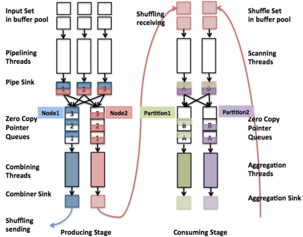
Figure 5: Distributed aggregation in PC.

1. The producing stage. In this stage, a sequence of TCAP operations that end in an AGGREGATE operation are used to create PipelineJobStage, which is realized as a list of pipelined stages, where each stage corresponds to a TCAP operation. A replica of the list of pipelined stages is created for each of the $N$ so-called pipelining threads dedicated to implementing the producing stage on each of the backend worker processes. The thread assigned to each of those pipelines begins by allocating a PC Vector <Handle <Map <Object, Object>>> on an output page. This page will serve as the pipe sink. The pipe sink is the location where the data produced by the pipeline are stored. In this way the PC object model is used to store the results from the producing stage, so that they can be sent over the network and used at the other side with no serialization/deserialization.

Once the pipe sinks have been allocated, the system begins assigning input pages to each of the pipelining threads. Each input page was itself produced as the result of a previous JobStage, or else created by users, both of which needs to be loaded from the storage. Hence all pages are themselves organized using the PC object model. Thus, each input page will itself contain a Vector <Handle <Object>>, or another standard PC container type. During the producing stage, vectors of PC Handles are repeatedly loaded from each input page, and each is used to create a vector list that is pushed through the list of pipeline stages.

Ultimately, pushing a vector list through the pipeline stages results in an output vector list that contains a vector of keys and a vector of values associated with those keys that need to be aggregated. For each (key, value) pair, first the key is hashed to a particular hash partition—the hash partition determines which of the Map objects in the Vector <Handle <Map <Object, Object>>> stored on the output page will receive the pair, and which machine will house the final aggregation for all instances of the key. Once the hash partition has been determined, the pair is added to the associated Map in the pipe sink (if a particular key is already there, the existing value is added to the new value, and the result is used to replace the existing value).

At the same time, $K$ different combining threads are running in each backend worker process. When a page containing a Vector <Handle <Map <Object, Object>>> becomes full, the thread running the associated PipelineJobStage allocates a new pipe sink, and the filled page is added to the queue of completed pages to be processed. There is one such queue associated with each of the $K$ combining threads. We call each such queue a zero copy pointer queue because the entire page of PC Objects is passed from a pipelining thread to each of the combining threads as a pointer, with no PC Object movement.

Each combining thread is assigned one or more hash partitions. When a combining thread is associated with a hash partition, it is responsible for aggregating all of the Maps produced by local pipelining threads that were associated with that hash partition. The result is a Map containing data for that one hash partition. Since each combining thread can be assigned more than one hash partition that will be sent to the same destination machine, the combining thread also produces a Vector <Handle <Map <Object, Object>>> that is referred to as a combining sink. Each Map in the Vector is associated with one hash partition. This object is stored on a thread-local combiner page whose size is automatically tuned by the system.

2. The consuming Stage. Once a combiner page becomes full, the page is directly sent to the worker node housing the backend worker processes tasked with processing the set of hash partitions on the page. This communication is referred to as a shuffle. Compression is used to reduce the shuffle data size and save on network cost. When a worker node receives a page during the shuffle, one of a pool of scanning threads will look at the Vector <Handle <Map <Object, Object>>> object contained in the page, and then add a pointer to the page to each of the queues associated with the $M$ aggregation threads. These are the threads that are tasked with final processing of all of the various hash partitions. Each aggregation thread is responsible for aggregating exactly one hash partition, and so $M$ is the total number of hash partitions processed by a given backend worker process. An aggregation thread has an output page housing its aggregation sink. The aggregation sink is a Map <Object, Object> that stores the portion of the data that it aggregates.

In PC, all of the “magic” parameters such as the number of hash partitions $M$, the number of pipelining threads $N$, the number of combining threads for each remote node $K$, the combiner page size, and the aggregation page size are all automatically determined at run-time to maximize memory utilization, network utilization and CPU utilization. The details are omitted here and will be discussed in a separate paper.

D.3 Hash Partition Join

We now briefly describe how PC implements a distributed equi-join of $n$ different sets using a hash-partition strategy. That is, imagine that $t$ = $\langle t_{1},t_{2},...,t_{n}\rangle$ is a tuple formed by taking one item from each of the $n$ sets. Let $key(t_{i})$ denote the join key of $t_{i}$. Then an $n$-way equi-join requires that in order for $t$ to be in the output set, it must be the case that $key(t_{i})=key(t_{j})$ forall $i,j$.

In PC, such an operation is broken into $2n$ JobStages. The first $n$ JobStages are PipelineJobStages hashing and repartitioning each of the $n$ sets, so that all of the data with the same join key value must be co-located on the same machine. The next $n-1$ JobStages are BuildHashTableJobStages that build hash tables for all of the entries in $n-1$ of those sets. The last JobStage is also a PipelineJobStage that scans the last set and probes the constructed hash tables.

In more detail, the three types of stages are:

1. The data repartition stages. This class of JobStages are PipelineJobStages. It is similar to the producing stage in distributed aggregation, with one key difference. Rather than using a Vector <Handle <Map <Object, Object>>> to store (key, value) pairs where the value is the result obtained by aggregating a set of data with the same key, the pipe sink used is instead a Vector <Handle <Map <unsigned_t, Vector <Object>>>> data structure. Here, the unsigned_t is a hash value produced by a TCAP HASH operation over the input object’s join key, and the Vector <Object> is a list of objects with the same hash value. When a new object with the same hash key is found during pipelined processing or during combining, rather than aggregating, the new object is instead inserted into the inner Vector <Object> data structure that contains a set of objects with the same hash key. Note that after the data repartition job stages completes, all of the data from all of the sets will have been repartitioned, so that all of the data with the same join key will be co-located on the same machine.

2. The hash table building stages. These JobStages are BuildHashTableJobStages, which are similar to the consuming job stage in aggregation, except that again, rather than aggregating, the goal is to build up Vectors of objects, stored in various Map data structures (one for each aggregation thread), where the Vector of objects associated with a particular unsigned_t contains all of the objects in a set whose join key hashes to that particular unsigned_t value. As a result of this class of JobStages, the contents of $n-1$ of the input sets will be stored precisely as required.

3. The hash join stage. This JobStage is also a PipelineJobStage. It runs over the last set (the one that was not hashed as part of join stage 2), and output results to the next JobStage (through shuffling) or an Output sink (e.g. write to storage as final results). Now imagine that we are processing the last dataset, after shuffling. At this point, all of the other sets have been stored in Map <unsigned_t, Vector <Object>> objects. As we process the final set, the hash value for each object is used to probe the Map associated with each of the other $n-1$ sets. If a match is found in each one of those other $n-1$ sets, then one or more entries in the output vector list are created to store the matches. The resulting vector sets are then pushed through a pipeline that post-processes the data in the vector list, likely checking to see if this was an actual match (and not just an accidental hash collision) and perhaps performing the processing necessary to prepare for the next join or aggregation. Note that if $m_{i}$ objects from the $i$th input set have the same unsigned_t hash value, then $\prod_{i}m_{i}$ entries in a vector set will be created as a result of these hash table probes.

References

- [1] Dl4j. https://deeplearning4j.org/. Accessed Sept 27, 2017.
- [2] Eigen. http://eigen.tuxfamily.org/index.php?title=Main_Page. Accessed Oct 22, 2016.
- [3] Gsl - gnu scientific library. https://www.gnu.org/software/gsl/. Accessed Oct 22, 2016.
- [4] Mahout. http://mahout.apache.org. Accessed Oct 22, 2016.
- [5] Mahout samsara. https://mahout.apache.org/users/environment/out-of-core-reference.html. Accessed Oct 22, 2016.
- [6] Project tungsten: Bringing spark closer to bare metal. https://databricks.com/blog/2015/04/28/project-tungsten-bringing-spark-closer-to-bare-metal.html. Accessed Nov 1, 2017.
- [7] Scidb’s supported os. http://www.paradigm4.com/HTMLmanual/14.8/scidb_ug/pr01s01.html. Accessed Nov 1, 2017.
- [8] D. J. Abadi, P. A. Boncz, and S. Harizopoulos. Column-oriented database systems. Proceedings of the VLDB Endowment, 2(2):1664–1665, 2009.
- [9] M. Abadi, A. Agarwal, P. Barham, E. Brevdo, Z. Chen, C. Citro, G. S. Corrado, A. Davis, J. Dean, M. Devin, et al. Tensorflow: Large-scale machine learning on heterogeneous distributed systems. arXiv preprint arXiv:1603.04467, 2016.
- [10] Y. Ahmad and C. Koch. Dbtoaster: A sql compiler for high-performance delta processing in main-memory databases. Proceedings of the VLDB Endowment, 2(2):1566–1569, 2009.
- [11] A. Alexandrov et al. The Stratosphere platform for big data analytics. VLDBJ, 23(6):939–964, 2014.
- [12] A. Alexandrov, A. Kunft, A. Katsifodimos, F. Schüler, L. Thamsen, O. Kao, T. Herb, and V. Markl. Implicit parallelism through deep language embedding. In Proceedings of the 2015 ACM SIGMOD International Conference on Management of Data, pages 47–61. ACM, 2015.
- [13] M. Armbrust, R. S. Xin, C. Lian, Y. Huai, D. Liu, J. K. Bradley, X. Meng, T. Kaftan, M. J. Franklin, A. Ghodsi, et al. Spark sql: Relational data processing in spark. In Proceedings of the 2015 ACM SIGMOD International Conference on Management of Data, pages 1383–1394. ACM, 2015.
- [14] D. F. Bacon, N. Bales, N. Bruno, B. F. Cooper, A. Dickinson, A. Fikes, C. Fraser, A. Gubarev, M. Joshi, E. Kogan, et al. Spanner: Becoming a sql system. In Proceedings of the 2017 ACM International Conference on Management of Data, pages 331–343. ACM, 2017.
- [15] H. P. Barendregt et al. The lambda calculus, volume 2. North-Holland Amsterdam, 1984.
- [16] M. Bittorf, T. Bobrovytsky, C. C. A. C. J. Erickson, M. G. D. Hecht, M. J. I. J. L. Kuff, D. K. A. Leblang, N. L. I. P. H. Robinson, D. R. S. Rus, J. R. D. T. S. Wanderman, and M. M. Yoder. Impala: A modern, open-source sql engine for hadoop. In Proceedings of the 7th Biennial Conference on Innovative Data Systems Research, 2015.
- [17] S. M. Blackburn, R. Garner, C. Hoffmann, A. M. Khang, K. S. McKinley, R. Bentzur, A. Diwan, D. Feinberg, D. Frampton, S. Z. Guyer, et al. The dacapo benchmarks: Java benchmarking development and analysis. In ACM Sigplan Notices, volume 41, pages 169–190. ACM, 2006.
- [18] D. M. Blei, A. Y. Ng, and M. I. Jordan. Latent dirichlet allocation. Journal of machine Learning research, 3(Jan):993–1022, 2003.
- [19] R. D. Blumofe, C. F. Joerg, B. C. Kuszmaul, C. E. Leiserson, K. H. Randall, and Y. Zhou. Cilk: An efficient multithreaded runtime system. Journal of parallel and distributed computing, 37(1):55–69, 1996.
- [20] M. Boehm, M. W. Dusenberry, D. Eriksson, A. V. Evfimievski, F. M. Manshadi, N. Pansare, B. Reinwald, F. R. Reiss, P. Sen, A. C. Surve, et al. Systemml: Declarative machine learning on spark. Proceedings of the VLDB Endowment, 9(13):1425–1436, 2016.
- [21] M. Boehm, S. Tatikonda, B. Reinwald, P. Sen, Y. Tian, D. R. Burdick, and S. Vaithyanathan. Hybrid parallelization strategies for large-scale machine learning in systemml. Proceedings of the VLDB Endowment, 7(7):553–564, 2014.
- [22] P. A. Boncz, M. Zukowski, and N. Nes. Monetdb/x100: Hyper-pipelining query execution. In Cidr, volume 5, pages 225–237, 2005.
- [23] D. Borthakur. Hdfs architecture guide. HADOOP APACHE PROJECT http://hadoop. apache. org/common/docs/current/hdfs design. pdf, 2008.
- [24] S. Breß, B. Köcher, H. Funke, T. Rabl, and V. Markl. Generating custom code for efficient query execution on heterogeneous processors. arXiv preprint arXiv:1709.00700, 2017.
- [25] P. G. Brown. Overview of scidb: large scale array storage, processing and analysis. In Proceedings of the 2010 ACM SIGMOD International Conference on Management of data, pages 963–968. ACM, 2010.
- [26] Z. Cai, Z. J. Gao, S. Luo, L. L. Perez, Z. Vagena, and C. Jermaine. A comparison of platforms for implementing and running very large scale machine learning algorithms. In Proceedings of the 2014 ACM SIGMOD international conference on Management of data, pages 1371–1382. ACM, 2014.
- [27] P. Carbone, A. Katsifodimos, S. Ewen, V. Markl, S. Haridi, and K. Tzoumas. Apache flink: Stream and batch processing in a single engine. Bulletin of the IEEE Computer Society Technical Committee on Data Engineering, 36(4), 2015.
- [28] S. Chaudhuri. An overview of query optimization in relational systems. In Proceedings of the seventeenth ACM SIGACT-SIGMOD-SIGART symposium on Principles of database systems, pages 34–43. ACM, 1998.
- [29] W. Chen, M. Kifer, and D. S. Warren. Hilog: A foundation for higher-order logic programming. The Journal of Logic Programming, 15(3):187–230, 1993.
- [30] E. F. Codd. A data base sublanguage founded on the relational calculus. In Proceedings of the 1971 ACM SIGFIDET (now SIGMOD) Workshop on Data Description, Access and Control, pages 35–68. ACM, 1971.
- [31] T. P. P. Council. Tpc-h benchmark specification. Published at http://www. tcp. org/hspec. html, 21:592–603, 2008.
- [32] A. Crotty, A. Galakatos, K. Dursun, T. Kraska, U. Cetintemel, and S. B. Zdonik. Tupleware:" big" data, big analytics, small clusters. In CIDR, 2015.
- [33] L. Dagum and R. Menon. Openmp: an industry standard api for shared-memory programming. IEEE computational science and engineering, 5(1):46–55, 1998.
- [34] A. Dave, A. Jindal, L. E. Li, R. Xin, J. Gonzalez, and M. Zaharia. Graphframes: an integrated api for mixing graph and relational queries. In Proceedings of the Fourth International Workshop on Graph Data Management Experiences and Systems, page 2. ACM, 2016.
- [35] J. Dean and S. Ghemawat. Mapreduce: Simplified data processing on large clusters. Communications of the ACM, 51(1):107–113, 2008.
- [36] A. Ghoting, R. Krishnamurthy, E. Pednault, B. Reinwald, V. Sindhwani, S. Tatikonda, Y. Tian, and S. Vaithyanathan. SystemML: Declarative machine learning on mapreduce. In ICDE, pages 231–242, 2011.
- [37] J. E. Gonzalez, R. S. Xin, A. Dave, D. Crankshaw, M. J. Franklin, and I. Stoica. Graphx: Graph processing in a distributed dataflow framework. In OSDI, volume 14, pages 599–613, 2014.
- [38] G. Graefe. Encapsulation of parallelism in the Volcano query processing system, volume 19. ACM, 1990.
- [39] G. Graefe. The cascades framework for query optimization. IEEE Data Eng. Bull., 18(3):19–29, 1995.
- [40] W. Gropp, E. Lusk, N. Doss, and A. Skjellum. A high-performance, portable implementation of the mpi message passing interface standard. Parallel computing, 22(6):789–828, 1996.
- [41] D. Grossman, G. Morrisett, T. Jim, M. Hicks, Y. Wang, and J. Cheney. Region-based memory management in cyclone. ACM Sigplan Notices, 37(5):282–293, 2002.
- [42] S. Idreos, F. Groffen, N. Nes, S. Manegold, S. Mullender, M. Kersten, et al. Monetdb: Two decades of research in column-oriented database architectures. A Quarterly Bulletin of the IEEE Computer Society Technical Committee on Database Engineering, 35(1):40–45, 2012.
- [43] M. Jarke and J. Koch. Query optimization in database systems. ACM Computing surveys (CsUR), 16(2):111–152, 1984.
- [44] N. M. Josuttis. The C++ standard library: a tutorial and reference. Addison-Wesley, 2012.
- [45] L. V. Kale and S. Krishnan. Charm++: a portable concurrent object oriented system based on c++. In ACM Sigplan Notices, volume 28, pages 91–108. ACM, 1993.
- [46] Y. Klonatos, C. Koch, T. Rompf, and H. Chafi. Building efficient query engines in a high-level language. Proceedings of the VLDB Endowment, 7(10):853–864, 2014.
- [47] C. Lattner and V. Adve. Llvm: A compilation framework for lifelong program analysis & transformation. In Proceedings of the international symposium on Code generation and optimization: feedback-directed and runtime optimization, page 75. IEEE Computer Society, 2004.
- [48] C. A. Lattner. LLVM: An infrastructure for multi-stage optimization. PhD thesis, University of Illinois at Urbana-Champaign, 2002.
- [49] G. Lebanon. Metric learning for text documents. IEEE Transactions on Pattern Analysis and Machine Intelligence, 28(4):497–508, 2006.
- [50] H. Li and et al. Tachyon: Reliable, memory speed storage for cluster computing frameworks. In SOCC, pages 1–15, 2014.
- [51] L. Lu and et al. Lifetime-based memory management for distributed data processing systems. VLDB, 9(12):936–947, 2016.
- [52] X. Meng, J. Bradley, B. Yavuz, E. Sparks, S. Venkataraman, D. Liu, J. Freeman, D. Tsai, M. Amde, S. Owen, et al. Mllib: Machine learning in apache spark. The Journal of Machine Learning Research, 17(1):1235–1241, 2016.
- [53] D. Miller. A logic programming language with lambda-abstraction, function variables, and simple unification. Journal of logic and computation, 1(4):497–536, 1991.
- [54] E. Moggi. Computational lambda-calculus and monads. In Logic in Computer Science, 1989. LICS’89, Proceedings., Fourth Annual Symposium on, pages 14–23. IEEE, 1989.
- [55] F. Nagel, G. Bierman, and S. D. Viglas. Code generation for efficient query processing in managed runtimes. Proceedings of the VLDB Endowment, 7(12):1095–1106, 2014.
- [56] T. Neumann. Efficiently compiling efficient query plans for modern hardware. Proceedings of the VLDB Endowment, 4(9):539–550, 2011.
- [57] C. J. Newburn, B. So, Z. Liu, M. McCool, A. Ghuloum, S. D. Toit, Z. G. Wang, Z. H. Du, Y. Chen, G. Wu, et al. Intel’s array building blocks: A retargetable, dynamic compiler and embedded language. In Proceedings of the 9th Annual IEEE/ACM International Symposium on Code Generation and Optimization, pages 224–235. IEEE Computer Society, 2011.
- [58] K. Ousterhout, R. Rasti, S. Ratnasamy, S. Shenker, B.-G. Chun, and V. ICSI. Making sense of performance in data analytics frameworks. In NSDI, volume 15, pages 293–307, 2015.
- [59] S. Palkar, J. J. Thomas, A. Shanbhag, D. Narayanan, H. Pirk, M. Schwarzkopf, S. Amarasinghe, M. Zaharia, and S. InfoLab. Weld: A common runtime for high performance data analytics. In Conference on Innovative Data Systems Research (CIDR), 2017.
- [60] H. Pirk, O. Moll, M. Zaharia, and S. Madden. Voodoo-a vector algebra for portable database performance on modern hardware. Proceedings of the VLDB Endowment, 9(14):1707–1718, 2016.
- [61] J. Reinders. Intel threading building blocks: outfitting C++ for multi-core processor parallelism. " O’Reilly Media, Inc.", 2007.
- [62] J. Shi, Y. Qiu, U. F. Minhas, L. Jiao, C. Wang, B. Reinwald, and F. Özcan. Clash of the titans: Mapreduce vs. spark for large scale data analytics. Proceedings of the VLDB Endowment, 8(13):2110–2121, 2015.
- [63] S. Sikdar, K. Teymourian, and C. Jermaine. An experimental comparison of complex object implementations for big data systems. In Proceedings of the 2017 Symposium on Cloud Computing, SoCC ’17, pages 432–444. ACM, 2017.
- [64] M. Stonebraker, D. J. Abadi, A. Batkin, X. Chen, M. Cherniack, M. Ferreira, E. Lau, A. Lin, S. Madden, E. O’Neil, et al. C-store: a column-oriented dbms. In Proceedings of the 31st international conference on Very large data bases, pages 553–564. VLDB Endowment, 2005.
- [65] M. Stonebraker, P. Brown, A. Poliakov, and S. Raman. The architecture of scidb. In Scientific and Statistical Database Management, pages 1–16. Springer, 2011.
- [66] M. Stonebraker, L. A. Rowe, B. G. Lindsay, J. Gray, M. J. Carey, M. L. Brodie, P. A. Bernstein, and D. Beech. Third-generation database system manifesto. ACM sIGMOD record, 19(3):31–44, 1990.
- [67] Y. Tian, S. Tatikonda, and B. Reinwald. Scalable and numerically stable descriptive statistics in systemml. In Data Engineering (ICDE), 2012 IEEE 28th International Conference on, pages 1351–1359. IEEE, 2012.
- [68] M. Tofte and J.-P. Talpin. Region-based memory management. Information and computation, 132(2):109–176, 1997.
- [69] Y. Yu et al. Dryadlinq: A system for general-purpose distributed data-parallel computing using a high-level language. In OSDI, volume 8, pages 1–14, 2008.
- [70] M. Zaharia, M. Chowdhury, M. J. Franklin, S. Shenker, and I. Stoica. Spark: cluster computing with working sets. In USENIX HotCloud, pages 1–10, 2010.
- [71] M. Zaharia and et al. Resilient distributed datasets: A fault-tolerant abstraction for in-memory cluster computing. In NSDI, pages 2–15. USENIX, 2012.
- [72] M. Zukowski, P. A. Boncz, N. Nes, and S. Héman. Monetdb/x100-a dbms in the cpu cache. IEEE Data Eng. Bull., 28(2):17–22, 2005.
- [73] M. Zukowski, M. van de Wiel, and P. Boncz. Vectorwise: A vectorized analytical dbms. In Data Engineering (ICDE), 2012 IEEE 28th International Conference on, pages 1349–1350. IEEE, 2012.