Local eigenvalue statistics of one dimensional random nonselfadjoint pseudodifferential operators

Abstract.

We consider a class of one-dimensional nonselfadjoint semiclassical pseudo-differential operators, subject to small random perturbations, and study the statistical properties of their (discrete) spectra, in the semiclassical limit $h\to 0$. We compare two types of random perturbation: a random potential vs. a random matrix. Hager and Sjöstrand had shown that, with high probability, the local spectral density of the perturbed operator follows a semiclassical form of Weyl’s law, depending on the value distribution of the principal symbol of our pseudodifferential operator.

Beyond the spectral density, we investigate the full local statistics of the perturbed spectrum, and show that it satisfies a form of universality: the statistical only depends on the local spectral density, and of the type of random perturbation, but it is independent of the precise law of the perturbation. This local statistics can be described in terms of the Gaussian Analytic Function, a classical ensemble of random entire functions.

1. Introduction

The spectral analysis of linear operators defined on a Hilbert space is much more developed in the case of selfadjoint operators: one can then use powerful tools, like the spectral theorem, or variational methods. This fact has been very useful in mathematical physics, for example in quantum mechanics, where the "natural" operators are selfadjoint. However, nonselfadjoint operators also appear in mathematical physics as well, and deserve to be investigated. For instance, in quantum mechanics, the study of scattering systems naturally leads to the concept of quantum resonances, which appear as the (complex valued) poles of the analytic continuation of the scattering matrix (or of the resolvent of the Hamiltonian) into the "nonphysical sheet" of the complex energy plane. These resonances may also be obtained as bona fide eigenvalues of a nonselfadjoint operator, obtained from the initial selfadjoint Hamiltonian through a complex deformation [1]. Still in quantum mechanics, when considering the evolution of a "small system" in contact with a "large environment", one can be lead to express the effective dynamics of the small system through a nonselfadjoint Lindblad operator [32]. in classical statistical physics, the linear operator generating the evolution of the system are often nonselfadjoint: the Fokker-Planck, or the linearized Boltzmann equation typically contain convective as well as dissipative terms, leading to nonselfadjoint operators. In hydrodynamics, the operators appearing when linearizing the Navier-Stokes equation in the vicinity of some specific solution are generally not selfadjoint.

When studying evolution problems generated by linear operators, one is naturally lead to analyze the spectrum of that operator, be it selfadjoint or not. Yet, in the nonselfadjoint case, establishing a connection between the long time evolution and a spectrum of complex eigenvalues is not so obvious as in the selfadjoint case, since eigenstates do not form an orthonormal family. This difficulty of connecting spectrum and dynamics is linked with a related characteristics of nonselfadjoint operators, namely the possible strong instability of their spectrum with respect to small perturbations, a phenomenon nowadays commonly called "pseudospectral effect". Traditionally this spectral instability was considered as a drawback, since it can be at the source of immense numerical errors, see [13]. However, as we will see below, analyzing this instability can also exhibit interesting phenomena. Numerical analysis studies, e.g. by L.N. Trefethen [43], somewhat changed the perspective of this instability problem: they showed that considering the pseudospectrum of the (nonselfadjoint) operator — that is the region where the resolvent operator is large — is often more relevant than considering its spectrum, and can reveal important dynamical informations. As an example, when studying a certain class of nonlinear diffusion equations, Sandsteede-Scheel [37], Raphael-Zworski [36] and Galkowski [17] showed that the pseudospectrum of the (nonselfadjoint) linearization of the equation can explain the finite time blow-up of the solutions to the full nonlinear equation.

In physical situations, perturbation of the "pure" nonselfadjoint operator can originate from many different sources, most of them uncontrolled. Hence, it seems natural to set up a model of perturbation by random operators, and to investigate how the spectrum of our operator reacts upon the addition of such perturbations. The spectrum of the full operator thereby becomes random; in case the spectrum is discrete, it forms a random point process on the complex plane, which can be investiaged by probabilistic methods. This is what we will do in this article, for a particular class of "pure" nonselfadjoint operators. Not all nonselfadjoint operators enjoy the same level spectral instability: some operators are very sensitive, others are less so. The operators we will consider in this work are semiclassical pseudodifferential operators with complex valued symbols, and with some ellipticity assumption ensuring that the spectrum is discrete (at least in some region of the complex plane). In the semiclassical regime, the spectrum of such an operator is very sensitive to perturbations; quite often, the spectrum of the "pure" operator is localized along 1-dimensional curves, while the perturbed spectrum fill up the classical spectrum, which is a domain of $\mathbb{C}$. This "filling up" of the classical spectrum has been precisely studied in a series of works by Hager [22, 21], Sjöstrand [40, 39, 23], Bordeaux-Montrieux [4] (see also [7] for a similar phenomenon in the framework of Toeplitz operators on the 2-torus). These authors show that the randomly perturbed spectrum satisfies, with high probability, a complex valued version of Weyl’s law: the density of eigenvalues near a point $z_{0}$ inside the classical spectrum, is approximately given by $(2\pi h)^{-1}\,D(z_{0})$, where $D(z_{0})$ is the classical density at the "energy" $z_{0}$, associated with the principal symbol of our operator.

This Weyl’s law counts the eigenvalues in any macroscopic region of $\mathbb{C}$, so it describes the spectrum at the macroscopic scale. Since the mean density is of order $h^{-1}$, it is reasonable to think that the typical distance between nearest eigenvalues should be of order $h^{1/2}$, which we will call the microscopic scale. Our aim in this article is to investigate the distribution of eigenvalues at this microscopic scale, from a statistical point of view; in other words, we aim at studying the local spectral statistics of this family of randomly perturbed operators, in particular the type of statistical interaction between nearby eigenvalues; as a first result on this spectral statistics has been obtained by the second named author, who computed the 2-point correlation between the eigenvalues of our randomly perturbed operator [44]. In this article we will give an essentially complete description of this local statistics in terms of the zeros of certain Gaussian analytic functions, and prove a partial form of universality.

Before stating our result more precisely, and to motivate them, let us recall some background on the topic of spectral statistics, from a mathematical physics perspective. In the 1950s Wigner had the idea, when studying the spectra of nuclear Hamiltonians, to replace these complicated operators by large random matrices [46]. The random matrix model could not reproduce the large scale density fluctuations of the nuclear spectra, which depend on specific features of the system, but they could (empirically) reproduce the local statistical properties of the spectra, at the scale of the mean spacing between eigenvalues. Wigner and Dyson understood that these local statistical properties only depend on global symmetries of the Hamiltonian, like time reversal invariance, but not on the fine details of the nuclear Hamiltonian: these statistical properties were thus said to be universal [12]. In the 1980s, this universality conjecture was extended to simpler Hamiltonians, namely Laplacians on Euclidean domains with specific shapes: Bohigas-Giannoni-Schmidt observed that if the geodesic flow in the domain is "chaotic", then the local spectral statistics of the corresponding Laplacian correspond to Dyson’s Gaussian Orthogonal ensemble [3]. In parallel, a large variety of non-Gaussian random Hermitian matrix ensembles were developed and studied, notably the Wigner random matrices (all entries are i.i.d. non-Gaussian, up to Hermitian symmetry), for which the local spectral statistics was recently shown to be identical with that of the Gaussian ensembles [14].

How about nonselfadjoint operators? Various random ensembles of nonhermitian matrices have also been introduced in the theoretical physics literature. The main objective has been to understand the distribution of quantum resonances for various types of scattering or dissipative systems, see for instance [16, 48, 30, 19] (a short recent review can be found in [15]). For most of these models, the focus has been to derive the mean spectral density, without investigating the correlation between the eigenvalues. The "historical" nonhermitian random matrix model, for which the full eigenvalue statistics has been derived in closed form, is the complex Ginibre ensemble [18], where all entries are i.i.d. complex Gaussian; the nearby eigenvalues then exhibit a statistical repulsion between the nearby eigenvalues, similar to the case of Dyson’s GUE ensemble of hermitian matrices. For certain non-Gaussian ensembles, recent results [6] have been obtained on the eigenvalue distribution at the microscopic scale, but they still fail to prove the universality of the local statistics. Before coming to our work, let us mention a model studied recently by Capitaine and Bordenave [5] (see also [9]), namely the case of a large Jordan block perturbed by a random Ginibre matrix: the authors prove that most eigenvalues of the perturbed matrix lie close to the unit circle, but they also prove that the "outliers" (the rare eigenvalues away from the unit circle) are distributed like the zeros of a "hyperbolic" Gaussian analytic function (GAF). Our results will involve instead a "Euclidean" Gaussian analytic function, yet the mechanisms through which GAFs appear in these two models are very similar.

1.1. Presentation of the results for a simple model case

Before stating our results in full generality, we will illustrate them by first focussing on a simple case. Call $h\in]0,1]$ the effective Planck’s "constant", and consider the nonselfadjoint semiclassical harmonic oscilator

$$P_{h}\stackrel{{\scriptstyle\mathrm{def}}}{{=}}-h^{2}\partial_{x}^{2}+ix^{2}\quad\text{ on }L^{2}(\mathds{R})\,.$$ (1.1)

The (semiclassical) principal symbol of $P_{h}$ is given by the function

$$p(x,\xi)=\xi^{2}+ix^{2}\quad\text{on the phase space $\in\mathds{R}^{2}\ni\rho=(x,\xi)$.}$$ (1.2)

We call the set

$$\Sigma\stackrel{{\scriptstyle\mathrm{def}}}{{=}}\overline{p(\mathds{R}^{2})}\subset\mathds{C}\quad\text{the classical spectrum of $P_{h}$}.$$ (1.3)

Here $\Sigma$ is obviously the upper right quadrant of $\mathds{C}$. The spectrum of $P_{h}$ is purely discrete, and is contained in $\Sigma$ (actually, it is explicitly given by $\{z_{n}=e^{i\pi/4}h(n+1/2);\ n\in\mathds{N}\}$). Take $\Omega\Subset\overset{\circ}{\Sigma}$ an open subset. Then, for any $z=X+iY\in\Omega$, an important data for our construction will be the structure of the "energy shell" $p^{-1}(z)\subset\mathds{R}^{2}$. Since $p:\mathds{R}^{2}\to\mathds{C}$ is a local diffeomorphism for $z\in\Omega$, this energy shell made of discrete points; in the case of the harmonic oscillator, $p^{-1}(z)$ consists of the 4 points:

$$\rho^{1}_{+}=(Y^{1/2},-X^{1/2}),\,\rho^{2}_{+}=(-Y^{1/2},X^{1/2}),\,\rho^{1}_{-}=(Y^{1/2},X^{1/2}),\,\rho^{2}_{+}=(-Y^{1/2},-X^{1/2})\,.$$ (1.4)

We have labelled those points according to the sign of the Poisson bracket $\{\mathrm{Re\,}p,\mathrm{Im\,}p\}(\rho)=4x\xi$: at the points $\rho^{j}_{+}$ the bracket is negative, while at the points $\rho^{j}_{-}$ it is positive. From this bracket condition, one can construct [8, 10], for each $j=1,2$ a semiclassical family of functions $(e_{+}^{j}(z,h)\in L^{2}(\mathds{R}))_{h\in]0,1]}$, $\|e_{+}^{j}(z,h)\|=1$, satisfying

$$\|(P_{h}-z)e_{+}^{j}(z,h)\|=\mathcal{O}(h^{\infty}),$$ (1.5)

and such that $e_{+}^{j}(z,h)$ is microlocalized at the point $\rho^{j}_{+}(z)$. (Here and in the entire text, all norms without index are either norms in $L^{2}$ or in $\mathcal{B}(L^{2})$, the set of bounded linear operators $L^{2}\to L^{2}$). We call each family $(e_{+}^{j}(z,h))$ an $h^{\infty}$-quasimode of $P-z$, or for short a quasimode of $P-z$. Similarly, there exists quasimodes $e_{-}^{j}(z,h)\in L^{2}(\mathds{R})$ for the adjoint operator $(P_{h}-z)^{*}$, microlocalized at the points $\rho^{j}_{-}(z)$. From the quasimode equation (1.5) it is easy to exhibit an operator $Q$ of norm unity and a parameter $\delta=\mathcal{O}(h^{\infty})$, such that the perturbed operator $P_{h}+\delta Q$ has an eigenvalue at $z$ (for instance, if we call the error $r_{+}^{j}=(P_{h}-z)e_{+}^{j}$, we may take the rank 1 operator $\delta Q=-r_{+}^{j}\otimes(e^{j}_{+})^{*}$). The set $\Omega$ (and hence the full interior of $\Sigma$, since $\Omega$ was chosen arbitrarily) is thus a zone of strong spectral instability for $P_{h}$. For this reason $\overset{\circ}{\Sigma}$ is called the ($h^{\infty}$-)pseudospectrum of $P_{h}$.

Let us now explain how we construct random perturbations, following [23]. Let $\{e_{k}\}_{k\in\mathds{N}}$ denote an orthonormal basis of $L^{2}(\mathds{R})$ comprised out of the eigenfunctions of the nonsemiclassical harmonic oscillator $H=-\partial_{x}^{2}+x^{2}$, and let $\{v_{j}\}_{j\in\mathds{N}}$, $\{q_{jk}\}_{j,k\in\mathds{N}}$ be independent and identically distributed (i.i.d.) complex Gaussian random variables with expectation $0$ and variance $1$ (that is, with distribution $\mathcal{N}_{\mathds{C}}(0,1)$). Let $N(h)=C_{1}/h^{2}$, with $C_{1}>0$ large enough. We define two types of random operators $Q$:

1. A random, Ginibre-type matrix

   $$Q=M_{\omega}=\frac{1}{N(h)}\sum_{0\leq j,k<N(h)}q_{j,k}e_{j}\otimes e_{k}^{*}$$ (1.6)

2. A random (complex valued) potential

   $$Q=V_{\omega}=\frac{1}{N(h)}\sum_{0\leq j<N(h)}v_{j}e_{j}.$$

The coupling variable $\delta=\delta(h)$ will be assumed to be in the range

$$h^{M}\leq\delta\leq h^{\kappa},$$ (1.7)

where $\kappa>3$, and $M>\kappa$ is an arbitrarily large but fixed constant. Although the random operator $Q$ and $\delta$ depend on $h$, we will skip the dependence in our notations. We are interested in the spectrum of the perturbed operator

$$P_{h}^{\delta}=P_{h}+\delta Q,$$

where the random operator $Q$ is either $M_{\omega}$ or $V_{\omega}$. With probability exponentially close to $1$, $\|M_{\omega}\|_{\mathrm{HS}},\|V_{\omega}\|_{\infty}\leq Ch^{-1}$ [21, 23].

Our objective will be to study the spectrum of $P_{h}^{\delta}$ in a microscopic neighbourhood of some given point $z_{0}\in\Omega$. As explained in the previous section, the probabilistic Weyl’s law proved in [21, 23] shows that the mean density of eigenvalues near $z_{0}$ is of order $h^{-1}$, so we expect nearby eigenvalues to be at distances $\sim h^{1/2}$ from one another. In order to test the statistical interaction between nearby eigenvalues, we zoom to this scale $h^{1/2}$ at the point $z_{0}$, and define the rescaled spectral point process:

$$\mathcal{Z}_{h,z_{0}}^{Q}\stackrel{{\scriptstyle\mathrm{def}}}{{=}}\sum_{z\in\mathrm{Spec}(P_{h}+\delta Q)}\delta_{(z-z_{0})h^{-1/2}}\,.$$

Our main result is to show that, in the semiclassical limit $h\to 0$, this rescaled point process converges in distribution the point process formed by the zeros of a certain random analytic function. In order to state our result, we need to define the building block of these random analytic functions, which is the (Euclidean) Gaussian analytic function (GAF).

1.2. The Gaussian analytic function

Let $(\alpha_{n})_{n\in\mathds{N}}$ be independent and identically distributed normal complex Gaussian random variables, i.e. $\alpha_{n}\sim\mathcal{N}_{\mathds{C}}(0,1)$ for every $n\in\mathds{N}$. For a given $\sigma>0$, we consider the random entire series

$$g_{\sigma}(w)\stackrel{{\scriptstyle\mathrm{def}}}{{=}}\sum_{n=0}^{\infty}\alpha_{n}\frac{\sigma^{n/2}w^{n}}{\sqrt{n!}},\quad z\in\mathds{C}\,.$$ (1.8)

With probability one, this series converges absolutely on the full plane, and defines a Gaussian analytic function (GAF) on $\mathds{C}$: $g_{\sigma}$ is a random entire function, so that for any $n\in\mathds{N}$ and any $w_{1},\dots,w_{n}\in\mathds{C}$ the random vector $(g(w_{1}),\dots,g(w_{n}))$ is a centred complex Gaussian

$$(g_{\sigma}(w_{1}),\ldots,g_{\sigma}(w_{n}))\sim\mathcal{N}_{\mathds{C}}(0,\Gamma),$$ (1.9)

where the covariance matrix $\Gamma\in GL_{n}(\mathds{C})$ has the entries

$$\Gamma_{i,j}=\mathds{E}\left[g_{\sigma}(w_{i})\overline{g_{\sigma}(w_{j})}\right]\overset{\mathrm{def}}{=}K_{\sigma}(w_{i},\overline{w}_{j})=\exp(\sigma w_{i}\overline{w}_{j})\,.$$ (1.10)

The function $\mathds{C}^{2}\ni(u,v)\mapsto K_{\sigma}(u,\overline{v})$ is called the covariance kernel of the GAF $g_{\sigma}$, it completely determines its distribution. As a result, $K_{\sigma}$ also completely determines the distribution of

$$\mathcal{Z}_{g_{\sigma}}\stackrel{{\scriptstyle\mathrm{def}}}{{=}}\sum_{w\in g^{-1}_{\sigma}(0)}\delta_{w},$$

the random point process given by zeros of the GAF $g_{\sigma}$, see for instance [28]. In Section 6, we will review basic notions and results concerning zero point processes of random analytic functions, making the above statements more precise.

The GAF zero process has interesting geometric properties. Indeed, its covariance kernel shows that for any $w_{0}\in\mathds{C}$, the translated function $g_{\sigma}(w+w_{0})$ is equal in distribution to the function $e^{\sigma(w\bar{w}_{0}+|w_{0}|^{2})}g_{\sigma}(w)$, which has the same zeros as $g_{\sigma}(w)$: this implies that the zero process $\mathcal{Z}_{g_{\sigma}}$ is invariant by translation. The average density (1-point function) of $\mathcal{Z}_{g_{\sigma}}$ is thus constant over the plane, it is equal to $\sigma/\pi$ (see section 2.5.3). The linear dependence in $\sigma$ is coherent with the scaling covariance $g_{\sigma}(w)\stackrel{{\scriptstyle d}}{{=}}g_{1}(\sqrt{\sigma}w)$: dilating the zero process $\mathcal{Z}_{g_{1}}$ by $1/\sqrt{\sigma}$ multiplies the average density by $\sigma$.

Let us give a short historical background of the GAF. It has appeared before in the context of holomorphic representations of quantum mechanics, when investigating the properties of random states. In the framework of Toeplitz quantization on a compact Kähler manifold $M$, one defines a positive line bundle $L$ over $M$, and for any integer $N\geq 1$ a "quantum" Hilbert space $\mathcal{H}_{N}$ is formed by the holomorphic sections on the bundle $L^{\otimes N}$; the limit $N\to\infty$ is then a form of semiclassical limit. In the case of the 1-dimensional projective space $M=\mathds{C}P^{1}$, which is the phase space of the quantum spin, Hannay [24] defined a natural ensemble of random holomorphic sections in $\mathcal{H}_{N}$, and studied the point process formed by their zeros (topological constraints impose that any section has exactly $N$ zeros). He explained how to compute the $k$-point correlation function of this process, and computed explicitly the limit (after microscopic rescaling) of the 2-point correlation function, which coincides with the 2-point function of the GAF. A few years later, Bleher-Schiffman-Zelditch [2] proved that, for a general Toeplitz quantization $(M,L)$, the zeros of random holomorphic sections converge, when $N\to\infty$, to a universal process depending only on the dimension of $M$. In dimension $1$, this process is given by the zero process of the GAF.

We are now equipped to state our Theorem concerning the spectrum of $P_{h}^{\delta}$.

Theorem 1 (Complex harmonic oscillator).

Fix $z_{0}=X_{0}+iY_{0}\in\Omega\Subset\mathring{\Sigma}$, and define the classical density for the symbol $p(x,\xi)=\xi^{2}+ix^{2}$ at the points $\rho^{j}_{\pm}\in p^{-1}(z_{0})$:

$$\sigma(z_{0})\stackrel{{\scriptstyle\mathrm{def}}}{{=}}\frac{1}{|\{\mathrm{Re\,}p,\mathrm{Im\,}p\}(\rho_{\pm}^{j}(z_{0}))|}=\frac{1}{4\sqrt{X_{0}Y_{0}}}\,.$$

Let the perturbation $Q$ be either $M_{\omega}$ or $V_{\omega}$, and take $\delta$ as in (1.7). Then, for any bounded domain $O\Subset\mathds{C}$, we have the convergence in distribution of the spectral point processes:

$$\mathcal{Z}_{h,z_{0}}^{Q}\stackrel{{\scriptstyle d}}{{\longrightarrow}}\mathcal{Z}_{G_{z_{0},Q}}\quad\text{ on }O,\quad\text{ as }h\to 0.$$

(This convergence of point processes is explained in Thm 6). Here $\mathcal{Z}_{G_{z_{0},Q}}$ is the zero point process for the random entire function $G_{z_{0},Q}$ described below:

1. if the perturbation $Q=V_{\omega}$ then

   $$G_{z_{0},V}(w)=g^{1}_{z_{0}}(w)g^{2}_{z_{0}}(w),\quad w\in\mathds{C},$$

   where $g^{1}_{z_{0}},g^{2}_{z_{0}}$ are two independent copies of the GAF $g_{\sigma(z_{0})}$.

2. if $Q=V_{\omega}$ then

   $$G_{z_{0},M}(w)=\det\big{(}g_{z_{0}}^{i,j}(w)\big{)}_{1\leq i,j\leq 2},\quad w\in\mathds{C},$$

   where $g_{z_{0}}^{i,j}$, $1\leq i,j\leq 2$, are 4 independent copies of the GAF $g_{\sigma(z_{0})}$.

As we will explain below (see section 2.5.2), the convergence of point processes implies that all $k$-point measures converge as well to the limiting ones.

2. Main results – general framework

The above theorem can be generalized to a large class of 1-dimensional nonselfadjoint $h$-pseudodifferential operators, and with random perturbations which are not necessarily Gaussian. We first present the class of operators we will be dealing with.

2.1. Semiclassical framework

We begin by recalling the definition of the pseudospectrum of an operator, an important notion which quantifies its spectral instability.

For $P:L^{2}\to L^{2}$, a densely defined closed linear operator with resolvent set $\rho(P)$ and spectrum $\mathrm{Spec}(P)=\mathds{C}\backslash\rho(P)$. For any $\varepsilon>0$, we define the $\varepsilon$-pseudospectrum of $P$ by

$$\mathrm{Spec}_{\varepsilon}(P)\stackrel{{\scriptstyle\mathrm{def}}}{{=}}\mathrm{Spec}(P)\cup\{z\in\rho(P);\|(P-z)^{-1}\|>\varepsilon^{-1}\}.$$ (2.1)

When $\varepsilon$ is small, the set (2.1) describes a region of spectral instability of the operator $P$, since any point in the $\varepsilon$-pseudospectrum of $P$ lies in the spectrum of a certain $\varepsilon$-perturbation of $P$ [13]. Indeed, $\mathrm{Spec}_{\varepsilon}(P)$ can also be defined by

$$\mathrm{Spec}_{\varepsilon}(P)=\bigcup_{\begin{subarray}{c}Q\in\mathcal{B}(L^{2})\\ \lVert Q\rVert<1\end{subarray}}\mathrm{Spec}(P+\varepsilon Q).$$ (2.2)

A third, equivalent definition of the $\varepsilon$-pseudospectrum of $P$ is via the existence of approximate solutions to the eigenvalue problem $P-z$:

$$z\in\mathrm{Spec}_{\varepsilon}(P)\Longleftrightarrow\exists u_{z}\in D(P)\text{ s.t. }\|(P-z)u_{z}\|<\varepsilon\|u_{z}\|,$$ (2.3)

where $D(P)$ denotes the domain of $P$. Such a state $u_{z}$ is called an $\varepsilon$-quasimode or simply a quasimode.

Next, let us fix the type of unperturbed operators we will consider in this paper. We will use the notation $\rho=(x,\xi)\in\mathds{R}^{2}$ for phase space points. We start by considering an order function $m\in\mathcal{C}^{\infty}(\mathds{R}^{2};[1,\infty[)$:

$$\exists C_{0}\geq 1,\leavevmode\nobreak\ \exists N_{0}>0:\quad m(\rho)\leq C_{0}\langle\rho-\mu\rangle^{N_{0}}m(\rho),\quad\forall\rho,\mu\in\mathds{R}^{2},$$ (2.4)

with the usual notation $\langle\rho-\mu\rangle\stackrel{{\scriptstyle\mathrm{def}}}{{=}}\sqrt{1+|\rho-\mu|^{2}}$. To this order function is associated a semiclassical symbol class (cf [11, 47]):

$$S(\mathds{R}^{2},m)=\left\{q\in\mathcal{C}^{\infty}(\mathds{R}^{2}_{\rho}\times]0,1]_{h});\leavevmode\nobreak\ \forall\alpha\in\mathds{N}^{2},\leavevmode\nobreak\ \exists C_{\alpha}:\right.\\ \left.|\partial^{\alpha}_{\rho}q(\rho;h)|\leq C_{\alpha}m(\rho),\leavevmode\nobreak\ \forall\rho\in\mathds{R}^{2},\ \forall h\in]0,1]\right\}.$$ (2.5)

We assume that the symbol $p\in S(\mathds{R}^{2},m)$ is "classical", namely it satisfies an asymptotic expansion in the limit $h\to 0$:

$$p(\rho;h)\sim p_{0}(\rho)+hp_{1}(\rho)+\dots\quad\text{in }S(\mathds{R}^{2},m),$$ (2.6)

where each $p_{j}\in S(\mathds{R}^{2},m)$ is independent of $h$. In this case we call $p_{0}$ the (semiclassical) principal symbol of $p$. We then define two subsets of $\mathds{C}$ associated with $p_{0}$:

$$\Sigma\stackrel{{\scriptstyle\mathrm{def}}}{{=}}\overline{p_{0}(\mathds{R}^{2})}\subset\mathds{C},\qquad\Sigma_{\infty}\stackrel{{\scriptstyle\mathrm{def}}}{{=}}\{z\in\Sigma;\leavevmode\nobreak\ \exists(\rho_{j})_{j\geq 1}\text{ s.t. }|\rho_{j}|\to\infty,\leavevmode\nobreak\ p_{0}(\rho_{j})\to z\}.$$ (2.7)

$\Sigma$ is the classical spectrum of the operator $P_{h}$ defined below. Furthermore, we suppose that the principal symbol $p_{0}$ is elliptic at some point $z_{out}\in\mathds{C}\backslash\Sigma$:

$$\exists C_{0}>0,\quad|p_{0}(\rho)-z_{out}|\geq m(\rho)/C_{0},\quad\forall\rho\in\mathds{R}^{2}.$$ (2.8)

For $h\in]0,1]$ we let $P_{h}$ denote the $h$-Weyl quantization of the symbol $p$,

$$P_{h}u(x)=p^{w}(x,hD_{x};h)u(x)=\frac{1}{2\pi h}\iint\mathrm{e}^{\frac{i}{h}(x-y)\cdot\xi}\,p\left(\frac{x+y}{2},\xi;h\right)u(y)dyd\xi,$$ (2.9)

which makes sense for $u\in\mathcal{S}(\mathds{R}^{d})$ the Schwartz space. The closure of $P_{h}$ as an unbounded operator on $L^{2}$, has domain $H(m)\stackrel{{\scriptstyle\mathrm{def}}}{{=}}(P_{h}-z_{out})^{-1}(L^{2}(\mathds{R}))\subset L^{2}(\mathds{R})$, we will still denote this closed operator by $P_{h}$. Moreover, we will denote by $\|u\|_{m}\stackrel{{\scriptstyle\mathrm{def}}}{{=}}\|(P_{h}-z_{out})u\|$ the associated norm on $H(m)$.

Let $\widetilde{\Omega}\subset\mathds{C}\backslash\Sigma_{\infty}$ be open simply connected, not entirely contained in $\Sigma$, and such that $\overline{\widetilde{\Omega}}\cap\Sigma_{\infty}=\emptyset$. Then, the spectrum of $P_{h}$ inside $\widetilde{\Omega}$ satisfies the following properties in the semiclassical limit [21, 23]:

• for $h>0$ small enough, $\mathrm{Spec}(P_{h})\cap\widetilde{\Omega}$ is discrete

• for all $\varepsilon>0$, $\exists h(\varepsilon)>0$ such that

  $$\mathrm{Spec}(P_{h})\cap\widetilde{\Omega}\subset\Sigma+D(0,\varepsilon),\quad\forall 0<h<h(\varepsilon).$$ (2.10)

Here, $D(0,\varepsilon)\subset\mathds{C}$ denotes the open disc of radius $\varepsilon>0$ centred at $0$. In this work we will study the spectrum of small random perturbations of $P_{h}$, in the semiclassical limit $h\to 0$, in the interior of $\Sigma$.

2.2. Pseudospectrum and the energy shell

Let $\widetilde{\Omega}$ be as above and let

$$\Omega\Subset\widetilde{\Omega}\cap\mathring{\Sigma}\text{ be open, simply connected.}$$ (2.11)

Recall that $p_{0}$ is the principal symbol of $p$, see (2.6). We also assume that:

$$\text{for every }\rho\in p_{0}^{-1}(\overline{\Omega}),\ \text{the $1$-forms }dp_{0},d\overline{p_{0}}\text{ are linearly independent.}$$ (2.12)

Since the dimension $d=1$, this condition is equivalent to:

$$\text{ for every }\rho\in p_{0}^{-1}(\overline{\Omega}),\ \{\mathrm{Re\,}p_{0},\mathrm{Im\,}p_{0}\}\neq 0,$$ (2.13)

where $\{\cdot,\cdot\}$ denotes the Poisson bracket of the two functions:

$$\{p,q\}(\rho)\stackrel{{\scriptstyle\mathrm{def}}}{{=}}\partial_{\xi}p(\rho)\,\partial_{x}q(\rho)-\partial_{\xi}q(\rho)\,\partial_{x}p(\rho),\qquad\rho=(x,\xi)\in\mathds{R}^{2}\,.$$

It was observed by Dencker, Sjöstrand and Zworski [10], and Sjöstrand [41] that since $\Omega$ is relatively compact and simply connected, (2.12), or equivalently (2.13), implies that there exists $J\in\mathds{N}^{*}$ depending only on $\Omega$, so that for any $z\in\Omega$, the "energy shell" $p_{0}^{-1}(z)$ consists of exactly $2J$ points:

$$\begin{split}p_{0}^{-1}(z)=\{\rho_{\pm}^{j}(z);j=1,\dots,J\},&\text{ with }\pm\{\mathrm{Re\,}p,\mathrm{Im\,}p\}(\rho_{\pm}^{j}(z))<0,\\ &\rho_{\pm}^{i}(z)\neq\rho_{\pm}^{j}(z)\ \text{ if }\ i\neq j,\end{split}$$ (HYP)

and the points $\rho_{\pm}^{j}(z)\in\mathds{R}^{2}$ depend smoothly on $z$.

We shall make the further (generic) assumption

$$\forall z\in\Omega,\quad x_{\pm}^{i}(z)\neq x_{\pm}^{j}(z)\ \text{ if }\ i\neq j\,,$$ (HYP-x)

which will play a role when studying the perturbation by a random potential.

It was shown by Davies [8] and Dencker, Sjöstrand and Zworski [10] that (HYP) implies, for each $z\in\Omega$ and each $j=1,\ldots,J$, the existence of an $h^{\infty}$-quasimode for the problem $P_{h}-z$ (resp. $(P_{h}-z)^{*}$), microlocalized on $\rho_{+}^{j}(z)$ (resp. $\rho_{-}^{j}(z)$): there exist $e_{\pm}^{j}=e_{\pm}^{j}(x,z;h)\in L^{2}(\mathds{R})$, $\|e_{\pm}^{j}\|=1$, such that

$$\|(P_{h}-z)e_{+}^{j}\|=\mathcal{O}(h^{\infty})\quad\text{and}\quad\mathrm{WF}_{h}(e_{+}^{j})=\{\rho_{+}^{j}(z)\},$$ (2.14)

respectively

$$\|(P_{h}-z)^{*}e_{-}^{j}\|=\mathcal{O}(h^{\infty})\quad\text{and}\quad\mathrm{WF}_{h}(e_{-}^{j})=\{\rho_{-}^{j}(z)\}.$$ (2.15)

Recall that, for $u=(u(h))_{h\in]0,1]}$ a bounded family in $L^{2}$, its semiclassical wavefront set $\mathrm{WF}_{h}(u)$ is defined by

$$\mathrm{WF}_{h}(u)\stackrel{{\scriptstyle\mathrm{def}}}{{=}}\complement\left\{(x,\xi)\in T^{*}\mathds{R};\leavevmode\nobreak\ \exists a\in\mathcal{C}_{c}^{\infty}(T^{*}\mathds{R}),\leavevmode\nobreak\ a(x,\xi)=1,\leavevmode\nobreak\ \lVert a^{w}(x,hD_{x})u(h)\rVert_{L^{2}}=\mathcal{O}(h^{\infty})\right\}$$

where $a^{w}$ denotes the Weyl quantization of $a$.

In view of the characterisation (2.3) of the pseudospectrum, we see that the assumption (2.12) implies that $\Omega$ is contained in the $h^{\infty}$-pseudospectrum of $P_{h}$, a spectrally highly unstable region.

2.3. Adding a random perturbation

We are interested in random perturbations of the operator $P_{h}$ which are given by either a random matrix or a random potential. We will construct those in the following way, which generalizes the construction made in section 1.1. We consider $\{e_{k}\}_{k\in\mathds{N}}$ the orthonormal eigenbasis of the (nonsemiclassical) harmonic oscillator $H=-\partial_{x}^{2}+x^{2}$ on $L^{2}(\mathds{R})$.

Remark 2.

The choice of this orthonormal basis is a convenient one for us. However, it will become clear later on in the text that what we need is a system of states (not necessarily orthonormal) such that the first $N(h)$ states microlocally cover a sufficiently large part of phase space, namely a neighbourhood of $p_{0}^{-1}(\Omega)$. We also need to avoid states which would have a large overlap with some of the quasimodes $e_{\pm}^{j}$, cf. (2.14), (2.15). We refer the reader in particular to the proofs of Propositions 47 and 54 below.

Let $\alpha$ be a complex valued random variable defined on some probability space $(\mathcal{M},\mathcal{F},\mathds{P})$, with the properties

$$\mathds{E}[\alpha]=0,\quad\mathds{E}[\alpha^{2}]=0,\quad\mathds{E}[|\alpha|^{2}]=1,\quad\mathds{E}[|\alpha|^{4+\epsilon_{0}}]<+\infty,$$ (2.16)

where $\varepsilon_{0}>0$ is an arbitrarily small but fixed constant. Here, $\mathds{E}[\cdot]$ denotes the expectation with respect to the probability measure $\mathds{P}$. The Markov inequality implies the following tail estimate: there exists a constant $\kappa_{\alpha}>0$ such that

$$\mathds{P}[|\alpha|\geq\gamma]\leq\kappa_{\alpha}\,\gamma^{-(4+\varepsilon_{0})},\quad\forall\gamma>0.$$ (2.17)

Remark 3.

For instance, a complex centred Gaussian random variable as in eq. (1.8) satisfies the above assumptions.

Random Matrix. Let $N(h)=C_{1}/h^{2}$, $C_{1}>0$ large enough (we’ll be more precise about this condition later). Let $q_{j,k}$, $0\leq j,k<N(h)$ be independent copies of the random variable $\alpha$ satisfying the conditions (2.16). We consider the "random matrix"

$$M_{\omega}=\frac{1}{N(h)}\sum_{0\leq j,k<N(h)}q_{j,k}\,e_{j}\otimes e_{k}^{*},$$ (RM)

where $e_{j}\otimes e_{k}^{*}u=(u|e_{k})e_{j}$ for $u\in L^{2}(\mathds{R})$. For some coupling parameter $0<\delta\ll 1$, we define the randomly perturbed perturbed operator

$$P^{\delta}_{M}=P_{h}+\delta M_{\omega}.$$ (2.18)

Random Potential. Take $N(h)=C_{1}/h^{2}$, $C_{1}>0$ as above. Let $v_{j}$, $0\leq j<N(h)$ be independent copies of the random variable $\alpha$. Still using the same orthonormal family $(e_{k})_{k\in\mathds{N}}$, we define the random function

$$V_{\omega}=\frac{1}{N(h)}\sum_{0\leq j<N(h)}v_{j}\,e_{j}.$$ (RP)

For $0<\delta\ll 1$, write the perturbed operator

$$P^{\delta}_{V}=P_{h}+\delta V_{\omega}.$$ (2.19)

We call this perturbation a "random potential", eventhough $V_{\omega}$ is complex valued. When we consider this type of perturbation, we will make the additional symmetry assumption:

$$p(x,\xi;h)=p(x,-\xi;h).$$ (SYM)

This hypothesis implies that we can group the points $\rho_{\pm}^{j}$ forming $p_{0}^{-1}(z)$, see (HYP), such that $\rho_{\pm}^{j}=(x^{j},\pm\xi^{j})$; as a result, the centres of microlocalization of the quasimodes $e_{+}^{j}$ and $e_{-}^{j}$ are located on the same fibre $T^{*}_{x^{j}}\mathds{R}=\{(x_{j},\xi),\,\xi\in\mathds{R}\}$.

Remark 4.

We could relax the assumption (SYM) into requiring this symmetry only at the level of the principal symbol, i.e. $p_{0}(x,\xi)=p_{0}(x,-\xi)$. However, for the simplicity of the presentation we prefer to make the above stronger hypothesis.

Restricting to bounded perturbations. For both types of perturbations, it will be easier for us to restrict the random variables to large discs $D(0,C/h)$, i.e. assume that

$$|v_{i}|,\leavevmode\nobreak\ |q_{i,j}|\leq C/h,\quad 0\leq i,j<N(h),\quad\text{for some $C>0$ sufficiently large}.$$ (2.20)

This restriction induces the boundedness of the perturbations $M_{\omega}$, $V_{\omega}$. Using (2.17) to estimate the probability of this restriction, we deduce that the boundedness of the perturbations occurs with high probability. Namely, there exists $C_{2}>0$ such that, for the random matrix,

$$\mathds{P}\big{[}\|M_{\omega}\|_{HS}\leq Ch^{-1}\big{]}\geq 1-C_{2}h^{\varepsilon_{0}},$$ (2.21)

where $\|M_{\omega}\|_{HS}$ denotes the Hilbert-Schmidt norm of $M_{\omega}$. Respectively, in the case of the random potential,

$$\mathds{P}\big{[}\|V_{\omega}\|_{\infty}\leq Ch^{-1}\big{]}\geq 1-C_{2}h^{2+\varepsilon_{0}}.$$ (2.22)

We will take the coupling parameter $\delta$ as in (1.7).

We will see in Section 5 that the spectra of $P^{\delta}_{M}$ and $P^{\delta}_{V}$ in $\Omega$ are purely discrete. The principal aim of this paper is to show that the statistical properties of these spectra, in a microscopic neighbourhood of any $z_{0}\in\Omega$, are universal, in a sense that we will specify later on.

Since $p_{0}-z$ is elliptic for every $z\in\mathds{C}\backslash\Sigma$, we have that the resolvent norm $\|(P_{h}-z)^{-1}\|=\mathcal{O}(1)$, uniformly as $h\to 0$. Therefore, in view of the characterisation (2.2) of the pseudospectrum, the spectra of $P^{\delta}_{M}$ and $P^{\delta}_{V}$ are contained in any neighbourhood $\Sigma+D(0,\epsilon)$, for any given $\epsilon>0$ and $h>0$ small enough. Moreover, since $\Omega\Subset\mathring{\Sigma}$, we will not feel the effects of the boundary of $\Sigma$; we will simply say that $\Omega$ lies in the bulk of the spectrum of the perturbed operator.

2.4. Probabilistic Weyl’s law and local statistics

In a series of works by Hager [22, 21, 23] and Sjöstrand [40, 39], the authors considered randomly perturbed operators $P^{\delta}$ as given in (2.18) and (2.19). Under more restrictive assumptions on the random variables than (2.16), they have shown the following result.

Theorem 5 (Probabilistic Weyl’s law).

Let $\Omega$ be as in (2.11), (2.12). Let $\Gamma\Subset\Omega$ be open with $\mathcal{C}^{2}$ boundary. Let $P^{\delta}$ be either of the randomly perturbed operators $P^{\delta}_{M}$ or $P^{\delta}_{V}$ with $\delta$ as in (1.7) with $\kappa>0$ sufficiently large. Then, in the limit $h\to 0$,

$$\#\big{(}\mathrm{Spec}(P^{\delta})\cap\Gamma\big{)}=\frac{1}{2\pi h}\left(\iint_{p_{0}^{-1}(\Gamma)}dxd\xi+o(1)\right)\quad\text{with probability $\geq 1-Ch^{\eta}$},$$ (2.23)

for some fixed $\eta>0$.

Furthermore the authors give an explicit control over both the error term in Weyl’s law, and the error term in the probability estimate.

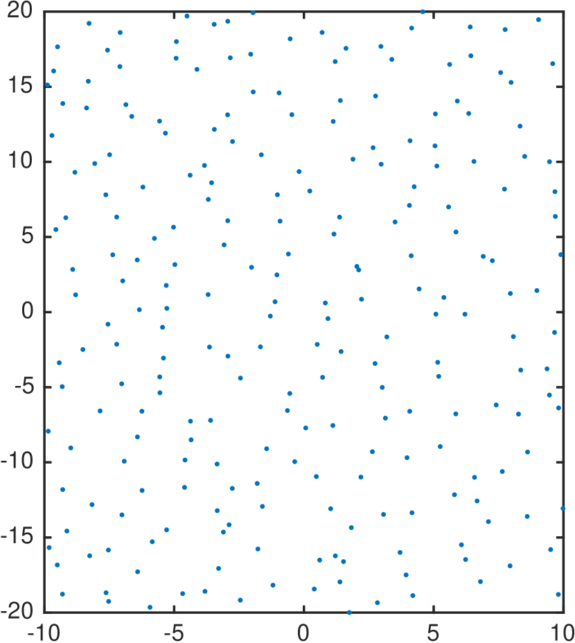
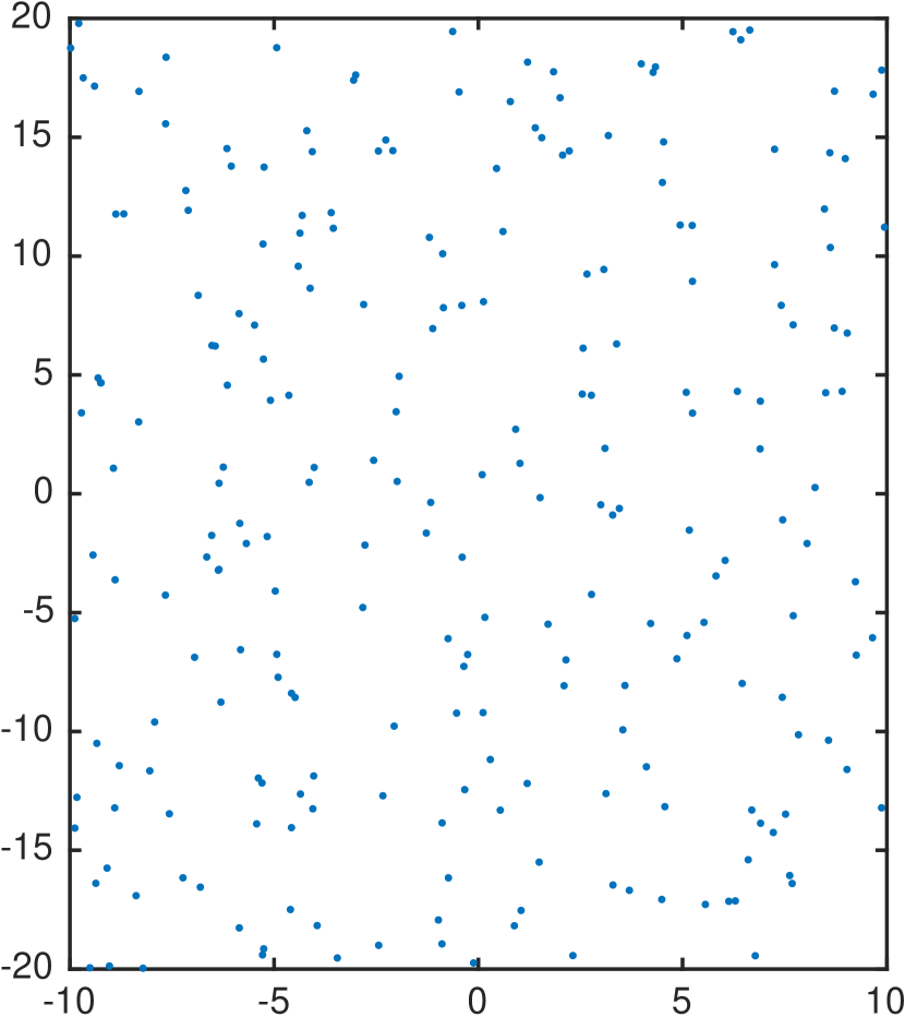
Figure 1. Numerically computed spectra of the operator $-h^{2}\partial_{x}^{2}+\mathrm{e}^{3ix}+\delta Q$ on $\mathbb{T}$, with $h=10^{-3}$ and $\delta=10^{-12}$. The left plot shows the case where $Q$ is given by a complex Gaussian random matrix and the right plot the case where $Q$ is given by a random potential as in (RP) with coefficients given by complex Gaussian random variables $\sim\mathcal{N}_{\mathds{C}}(0,1)$.

This probabilistic Weyl’s law shows that, with probability close $1$, the number of eigenvalues of the perturbed operator $P^{\delta}$ in any fixed compact subset of $\Omega$ is of order $\asymp h^{-1}$. Hence, the spectrum of $P^{\delta}$ will spread out across $\Omega$, with an average spacing between nearby eigenvalues of order $h^{1/2}$. Figure 1 illustrates this behaviour for some choice of perturbed operators $P^{\delta}_{M}$ and $P^{\delta}_{V}$. We observe in Figure 1 that in the case of $P^{\delta}_{V}$ (right plot), the distribution of the eigenvalues looks "less uniform" than in the case of $P^{\delta}_{M}$, including the presence of small clusters of eigenvalues.

To quantify this difference of "uniformity" between the spectra of $P^{\delta}_{M}$ and $P^{\delta}_{V}$, we study the local statistics of the eigenvalues, that is the statistics of the eigenvalues on the scale of their mean level spacing. For this purpose, we fix a point $z_{0}\in\Omega$. In both cases $Q=M_{\omega}$ and $Q=V_{\omega}$, we view the rescale the spectrum of the randomly perturbed operator $P^{\delta}_{Q}$ as a random point process

$$\mathcal{Z}_{h,z_{0}}^{Q}\stackrel{{\scriptstyle\mathrm{def}}}{{=}}\sum_{z\in\mathrm{Spec}(P^{\delta}_{Q})}\delta_{(z-z_{0})h^{-1/2}},\qquad Q=M_{\omega}\ \ \text{or}\ \ Q=V_{\omega},$$ (2.24)

where the eigenvalues are counted according to their algebraic multiplicities.

Notice that the rescaled eigenvalues $(z_{j}-z_{0})h^{-1/2}$ have a mean spacing of order $\asymp 1$. The principal aim of this paper is to show that, under the assumption (2.16) on the random coefficients, in the limit $h\to 0$ the correlation functions of the processes $\mathcal{Z}_{h,z_{0}}^{M}$ and $\mathcal{Z}_{h,z_{0}}^{V}$ are universal, in the sense that they

• depend only on the structure of the energy shell $p_{0}^{-1}(z)$ and on the type of random perturbation used, either $M_{\omega}$ or $V_{\omega}$;

• are independent of the random variables $q_{j,k}$ and $v_{j}$ used to define the random perturbations, as long as they satisfy (2.16).

Finally, let us stress once more that our results concern solely the eigenvalues in the bulk of the spectra of $P^{\delta}_{h}$, that is in the interior of the $h^{\infty}$-pseudospectrum of $P_{h}$. Near the boundary of the pseudospectrum, we expect the statistical properties of the eigenvalues to change drastically. It has been shown by the second author [45] in the case of a model operator, that the probabilistic Weyl’s law breaks down in the vicinity of $\partial\Sigma$, in fact, the density of eigenvalues explodes near that boundary.

2.5. Perturbation by a random potential

We begin with the case of the operator $P^{\delta}_{V}$, (2.19), perturbed by a random potential $V_{\omega}$. From the formula (HYP) defining the energy shell $p_{0}^{-1}(z)$, we find that the classical spectral density at the energy $z$ is given by

$$(p_{0})_{*}(|d\xi\wedge dx|)=\sum_{j=1}^{J}(\sigma_{+}^{j}(z)+\sigma_{-}^{j}(z))L(dz),\quad\sigma_{\pm}^{j}(z)=\frac{1}{\mp\{\mathrm{Re\,}p_{0},\mathrm{Im\,}p_{0}\}(\rho_{\pm}^{j}(z))}\,.$$ (2.25)

Here $|d\xi\wedge dx|$ denotes the measure induced by the symplectic volume form on $T^{*}\mathds{R}\cong\mathds{R}^{2}$. Each density $\sigma_{\pm}^{j}(z)>0$ is associated with the point $\rho^{j}_{\pm}$ of the energy shell. These densities depend smoothly on $z$.

If we additionally assume the symmetry hypothesis (SYM) and group the points such that $\rho_{\pm}^{j}=(x^{j},\pm\xi^{j})$, we find that $\sigma_{+}^{j}(z)=\sigma_{-}^{j}(z)$ for all $j=1,\ldots,J$.

2.5.1. Universal limiting point process

Let us now state our main theorem for the perturbed operators $P^{\delta}_{V}$. It provides the asymptotic behaviour of the rescaled spectral point processes $\mathcal{Z}^{V}_{h,z_{0}}$ in the semiclassical limit.

Theorem 6.

Let $\Omega\Subset\mathring{\Sigma}$ be as in (2.11), let $p$ be as in (2.6) satisfying (2.12) and (SYM). Fix $z_{0}\in\Omega$. Then, for any open, connected, relatively compact domain $O\Subset\mathds{C}$, we have that

$$\mathcal{Z}_{h,z_{0}}^{V}\stackrel{{\scriptstyle d}}{{\longrightarrow}}\mathcal{Z}_{G_{z_{0}}}\quad\text{ in }O,\quad\text{ as }h\to 0,$$

This convergence of point processes means that for any test function $\phi\in\mathcal{C}_{c}(O,\mathds{R})$,

$$\langle\mathcal{Z}_{h,z_{0}}^{V},\phi\rangle=\sum_{z\in\mathrm{Spec}(P^{\delta}_{h})}\phi((z-z_{0})h^{-1/2})\stackrel{{\scriptstyle d}}{{\longrightarrow}}\langle\mathcal{Z}_{G_{z_{0}}},\phi\rangle=\sum_{z\in G_{z_{0}}^{-1}(0)}\phi(z),\quad\text{ as }h\to 0\,.$$

Here $\mathcal{Z}_{G_{z_{0}}}$ is the zero point process for the random analytic function

$$G_{z_{0}}(z)=\prod_{j=1}^{J}g^{j}_{z_{0}}(z),\quad z\in\mathds{C},$$

where the $g^{j}_{z_{0}}$ are $J$ independent GAFs $g^{j}_{z_{0}}\sim g_{\sigma_{+}^{j}(z_{0})}$ (see section 1.2), with $\sigma_{+}^{i}(z_{0})$ the local spectral density computed in in (2.25).

For the reader’s convenience, in Section 6 we present a short review of the probabilistic notions used in this paper, such as convergence in distribution. The definition and basic properties of the GAFs have been presented in section 1.2.

This theorem tells us that at any given point $z_{0}\in\Omega$ in the bulk of the pseudospectrum, the local rescaled point process of eigenvalues is given, in the limit $h\to 0$, by the point process given by the zeros of the product of $J$ independent GAFs. Hence, this limiting point process is the superposition of $J$ independent point processes, each one generated by a GAF $g^{j}$. The latter only depends only on the part of the classical spectral density coming from the pair of points $\rho_{\pm}^{j}=(x^{j},\pm\xi^{j})$. In particular, this limiting process is independent of the specific probability distribution of the coefficients $(v_{j})$, or of the orthonormal family $(e_{j})$ used to generate the random potential $V_{\omega}$; this process only depends on cardinal $2J$ of the energy shell $p_{0}^{-1}(z)$ and of the local spectral densities $\{\sigma_{+}^{j}(z_{0}),\ j=1,\dots,J\}$.

It is known that the zero process of a single GAF exhibits a local repulsion between the nearby points (see the section 2.5.3). On the other hand, as a superposition of $J$ independent point processes, the limiting process $\mathcal{Z}_{G_{z_{0}}}$ authorizes the presence of clusters of at most $J$ points. In the next section we analyze this clustering by computing the correlations between the points of the process.

2.5.2. Scaling limit of the $k$-point measures

An explicit way to obtain information about the statistical interaction of $k$ nearby eigenvalues of $P^{\delta}_{V}$ is by analysing the $k$-point measures of the point process $\mathcal{Z}_{h,z_{0}}^{V}$, which quantify the correlations within $k$-point subsets of the point process. These are positive measures $\mu_{h}^{k,V,z_{0}}$ on $O^{k}\backslash\Delta$, where $O$ is as in Theorem 6 and $\Delta=\{z\in\mathds{C}^{k};\exists\leavevmode\nobreak\ i\neq j\leavevmode\nobreak\ \text{s.t. }z_{i}=z_{j}\}$ is a generalized diagonal set. These measures are defined through their action on an arbitrary test funtion $\phi\in\mathcal{C}_{c}(O^{k}\backslash\Delta,\mathds{R}_{+})$:

$$\begin{split}\mathds{E}\left[(\mathcal{Z}_{h,z_{0}}^{V})^{\otimes k}(\phi)\right]&=\mathds{E}\left[\sum_{z_{1},\dots,z_{k}\in\mathrm{Spec}(P^{\delta})}\phi\left((z_{1}-z_{0})h^{-1/2},\dots,(z_{k}-z_{0})h^{-1/2}\right)\right]\\ &\stackrel{{\scriptstyle\mathrm{def}}}{{=}}\int_{O^{k}\backslash\Delta}\phi(w)\,\mu_{h,z_{0}}^{k,V}(dw)\,.\end{split}$$ (2.26)

We have stamped out the diagonal $\Delta$ in order to avoid trivial self-correlations. When these $k$-point measures are absolutely continuous with respect to the Lebesgue measure on $\mathds{C}$, we call their densities the $k$-point functions.

Theorem 7.

Let $\mu_{h,z_{0}}^{k,V}$ be the $k$-point measure of $\mathcal{Z}_{h,z_{0}}^{V}$, defined in (2.26), and let $\mu^{k,V}_{z_{0}}$ be the $k$-point measure of the point process $\mathcal{Z}_{G_{z_{0}}}$, given in Theorem 6. Then, for any connected domain $O\Subset\mathds{C}$ and for all $\phi\in\mathcal{C}_{c}(O^{k}\backslash\Delta,\mathds{R}_{+})$,

$$\int_{O^{k}\backslash\Delta}\phi(w)\,\mu_{h,z_{0}}^{k,V}(dw)\longrightarrow\int_{O^{k}\backslash\Delta}\phi(w)\,\mu^{k,V}_{z_{0}}(dw),\quad h\to 0.$$

Moreover, $\mu^{k,V}_{z_{0}}$ is absolutely continuous with respect to the Lebesgue measure on $\mathds{C}$. Its density $d^{k,V}_{z_{0}}$ is given by the following formula:

$$d^{k,V}_{z_{0}}(w_{1},\ldots,w_{k})=\sum_{\begin{subarray}{c}\alpha\in\mathds{N}^{J},\\ \sum_{j}\alpha_{j}=k\end{subarray}}\sum_{\tau\in\mathfrak{S}_{k}}\frac{1}{\alpha!}\prod_{j=1}^{J}d^{\alpha_{j}}_{g_{j}}(w_{\tau(\alpha_{1}+\cdots+\alpha_{j-1}+1)},\dots,w_{\tau(\alpha_{1}+\cdots+\alpha_{j})})$$ (2.27)

where $\mathfrak{S}_{k}$ is the symmetric group of $k$ elements, and for all $1\leq j\leq J$ and all $r\in\mathds{N}^{*}$,

$$d_{g^{j}}^{r}(w)=\frac{\mathrm{perm}[C_{j}^{r}(w)-B_{j}^{r}(w)(A_{j}^{r})^{-1}(w)(B_{j}^{r})^{*}(w)]}{\det\pi A_{j}^{r}(w)},\ \ \text{while }d_{g^{j}}^{0}(w)\equiv 1\,.$$ (2.28)

Here, $\mathrm{perm}$ denotes the permanent of a matrix; $A_{j}^{r},B_{j}^{r},C_{j}^{r}$ are complex $r\times r$-matrices given by

$$(A_{j}^{r})_{n,m}=K^{j}(w_{n},\bar{w}_{m}),\quad(B_{j}^{r})_{n,m}=(\partial_{w}K^{j})(w_{n},\bar{w}_{m}),\quad(C_{j}^{r})_{n,m}=(\partial^{2}_{w\bar{w}}K^{j})(w_{n},\bar{w}_{m}),$$

where $K^{j}(w,\bar{w})=\exp(\sigma_{+}^{j}(z_{0})w\bar{w})$ is the covariance function of the GAFs $g^{j}_{z_{0}}$ appearing in Thm 6.

The function $d_{g^{j}}^{r}(z)$ in (2.28) is the $r$-point function for the zero process of the Gaussian analytic function $g^{j}$. Thm 7 tells us that the limiting $k$-point measures admit densities with respect to the Lebesgue measure, and that those can be determined by concatenating the $r$-point functions, for $1\leq r\leq k$, of each GAF $g^{j}$.

A result by Nazarov and Sodin [34, Theorem 1.1] implies the following estimate for the $r$-point densities of a single GAF.

Proposition 8.

[34] Let $O\Subset\mathds{C}$ be a compact set. Let $(g^{j}=g^{j}_{z_{0}})_{1\leq j\leq J}$ be the GAFs appearing in Thm 6, and let $d^{r}_{g^{j}}(w)$, $1\leq r\leq k$, be as in (2.28). Then there exists a constant $C=C(r,g^{j},O)>1$ such that, for any configuration of pairwise distinct points $w_{1},\ldots,w_{k}\in O$,

$$C^{-1}\prod_{i<j}|w_{i}-w_{j}|^{2}\leq d_{g^{j}}^{r}(w_{1},\dots,w_{k})\leq C\prod_{i<j}|w_{i}-w_{j}|^{2}.$$

In formula (2.27) we see that if $k>J$, then each summand has at least one factor $d^{\alpha_{j}}_{g^{j}}$ has $\alpha_{j}\geq 2$. Hence, we immediately conclude from Thm 7 and Prop. 8 the following

Corollary 9.

Let $O\Subset\mathds{C}$ be a compact set, let $k>J$ and let $d^{k,V}_{z_{0}}(w)$ be as in (2.27). Then there exists a positive constant $C=C(r,O)$ such that, for any configuration of pairwise distinct points $w_{1},\ldots,w_{k}\in O$,

$$d^{k,V}_{z_{0}}(w_{1},\ldots,w_{k})\leq C\sum_{i<j}|w_{i}-w_{j}|^{2}.$$

We have seen by Theorem 7 that the limiting point process of the rescaled eigenvalues is given by the superposition of $J$ independent processes given by the zeros of independent Gaussian analytic functions. Due to this independence, $k$ points, each originating from a different GAF process, may approach each other without any statistical repulsion: this authorizes the formation of clusters of a most $J$ points. As a result, for $k\leq J$ the limiting $k$-point functions do not decay to zero as the distances between the $k$ points gets smaller. This behaviour is made explicit in the next section in the case $k=2$.

On the opposite, if $k>J$ then at least two points must originate from the same GAF process, and therefore repel each other quadratically when approaching. This is exactly what Corollary 9 tells us: the probability to find more than $J$ points close together decays quadratically with the distance. Therefore, finding clusters of more than $J$ eigenvalues very close together is very unlikely.

2.5.3. $2$-point correlation function

The $2$-point correlation function of a point process is defined by the $2$-point function, renormalized by the local $1$-point functions (or local average densities):

$$K^{2,Q}_{z_{0}}(w_{1},w_{2})=\frac{d^{2,Q}_{z_{0}}(w_{1},w_{2})}{d^{1,Q}_{z_{0}}(w_{1})d^{1,Q}_{z_{0}}(w_{2})},\quad w_{1}\neq w_{2}\in O,\quad Q=V_{\omega},\ M_{\omega}\,.$$

By Theorem 7, the limiting local $1$-point function $d^{1,V}_{z_{0}}(w)$ is a constant function, given by

$$d^{1,V}_{z_{0}}(w)=\sum_{j=1}^{J}\frac{\sigma_{+}^{j}(z_{0})}{\pi},\quad\forall w\in O.$$

This average density of eigenvalues (at the microscopic scale near $z_{0}$) exactly corresponds to the macroscopic density predicted by the probabilistic Weyl’s law in Theorem 5, see also (2.25).

The limiting $1$-point and $2$-point functions of the zero process generated by a single GAF $g_{\sigma}$ (see section 1.2) are given by

$$d^{1}_{g_{\sigma}}(w_{1})=\frac{\sigma}{\pi},\quad\text{respectively}\quad d^{2}_{g_{\sigma}}(w_{1},w_{2})=\Big{(}\frac{\sigma}{\pi}\Big{)}^{2}\kappa\Big{(}\frac{\sigma|w_{1}-w_{2}|^{2}}{2}\Big{)},$$

with the universal scaling function

$$\kappa(t)\stackrel{{\scriptstyle\mathrm{def}}}{{=}}\frac{(\sinh^{2}t+t^{2})\cosh t-2t\sinh t}{\sinh^{3}t},\quad\forall t\geq 0.$$ (2.29)

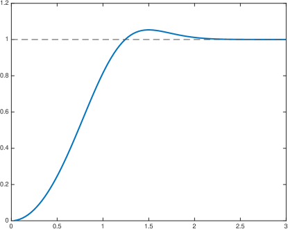
Figure 2. Plot of the scaling limit function $\kappa(t^{2})$, see (2.29).

The function $\kappa\left(\sigma|w_{1}-w_{2}|^{2}/2\right)$ describes the $2$-point correlation function of the zeros of the GAF $g_{\sigma}$. A remarkable property of this function is its isotropy: it only depends on the distance between the points $w_{1},w_{2}$. In Figure 2 we plot the function $t\mapsto\kappa(t^{2})$. This function behaves as $\kappa(t^{2})=t^{2}(1+\mathcal{O}(t^{4}))$ when $t\to 0$, which reflects the quadratic repulsion between the nearby zeros of $g_{\sigma}$. On the opposite, when $t\gg 1$ it converges exponentially fast to unity, showing a fast decorrelation between the zeros.

To our knowledge, the function $\kappa$ first appeared as the scaling limit $2$-point correlation function for the zeros of certain ensembles of random polynomials describing random spin states, see J.H. Hannay [24]. In the work by P. Bleher, B. Shiffman and S. Zelditch [2], $\kappa$ describes the scaling limit $2$-point correlation function for the zeros of random holomorphic sections of large powers of a positive Hermitian line bundle over a compact complex Kähler surface.

In the present work, $\kappa$ appears as a building block for the scaling limit $2$-point correlation function of the eigenvalues of $P_{V}^{\delta}$:

$$K^{2,V}_{z_{0}}(w_{1},w_{2})=1+\sum_{j=1}^{J}\frac{(\sigma_{+}^{j}(z_{0}))^{2}}{\left(\sum_{j=1}^{J}\sigma_{+}^{j}(z_{0})\right)^{2}}\left[\kappa\left(\frac{\sigma^{j}_{+}(z_{0})|w_{1}-w_{2}|^{2}}{2}\right)-1\right]$$ (2.30)

Let us study more closely this limiting $2$-point correlation function between the rescaled eigenvalues of $P^{\delta}_{V}$ near $z_{0}$:

Long range decorrelation: For $|w_{1}-w_{2}|\gg 1$, in the limit $h\to 0$, the $2$-point correlation function converges exponentially fast to unity

$$K^{2,V}_{z_{0}}(w_{1},w_{2})=1+\mathcal{O}\left(\mathrm{e}^{-\min\limits_{j}\sigma^{j}_{+}(z_{0})|w_{1}-w_{2}|^{2}}\right).$$

This shows that two points at distances $|w_{1}-w_{2}|\gg 1$ are statistically uncorrelated.

A weak form of repulsion: When $|w_{1}-w_{2}|\ll 1$, in the limit $h\to 0$, there is a weak form of repulsion between two nearby eigenvalues,

$$K^{2,V}_{z_{0}}(w_{1},w_{2})=1-\sum_{j=1}^{J}\frac{\sigma_{+}^{j}(z_{0})^{2}}{\big{(}\sum_{l=1}^{J}\sigma_{+}^{l}(z_{0})\big{)}^{2}}\Big{[}1-\frac{\sigma^{j}_{+}(z_{0})|w_{1}-w_{2}|^{2}}{2}+\mathcal{O}(|w_{1}-w_{2}|^{4})\Big{]}.$$ (2.31)

This formula shows that the probability to find two rescaled eigenvalues $w_{1},w_{2}$ at distance $\ll 1$ is smaller than the one to find them at large distances: pairs of rescaled eigenvalues show a weak repulsion at short distance. However, the correlation function does not converge zero when $|w_{1}-w_{2}|\to 0$, but to the positive value $1-\frac{\sum_{j=1}^{J}\sigma_{+}^{j}(z_{0})^{2}}{(\sum_{l=1}^{J}\sigma_{+}^{l}(z_{0}))^{2}}$. This weak repulsion can be explained by the fact that the random function $G_{z_{0}}$ is the product of $J$ independent GAFs: two zeros $w_{1},w_{2}$ will not repel each other if they originate from different GAFs, while they will repel quadratically if the come from the same GAF. The net result is this weaker form of repulsion. The larger the number of quasimodes $J$, the weaker this repulsion becomes, since two zeros $w_{1},w_{2}$ chosen at random will have a smaller chance to come from the same GAF.

In Figure 3 we compare the theoretical $2$-point correlation functions $K^{2,V}_{z_{0}}$ with the one obtained from numerical computations for two model operators on the torus $\mathbb{T}=\mathds{R}/(2\pi\mathds{Z})$:

$$P_{h,q}^{\delta}=-h^{2}\partial_{x}^{2}+\mathrm{e}^{-iqx}+\delta V_{\omega},\quad q=1,3,\quad x\in\mathbb{T}.$$ (2.32)

We took the parameters $h=10^{-3}$, $\delta=10^{-12}$, and the Gaussian random potential $V_{\omega}$ as in section 1.1. We use operators defined on $\mathbb{T}$ because they are numerically easier to diagonalize than operators defined on $\mathds{R}$. For each operator $P_{h,q}$, we computed 1000 realizations of the random potential to extract the correlation function.

The analysis of the principal symbols $p_{q,0}$ shows that the classical spectrum is, in both cases, given by $\Sigma=\mathds{R}_{+}+U(1)$. At the energy $z_{0}=1.6$ we selected, the operator $(P_{h,q}-z_{0})$ admits $J=2q$ quasimodes. Figure 3 compares the numerically obtained $2$-point correlation functions (shown as blue dots) of the operators $P_{h,1}^{\delta}$ (left) and $P_{h,3}^{\delta}$ (right), with the theoretical scaling limit $2$-point correlation described in (2.31). For the two operators, the theoretical curve fits quite well the numerical points, including in the short distance limit $|w_{1}-w_{2}|\ll 1$.

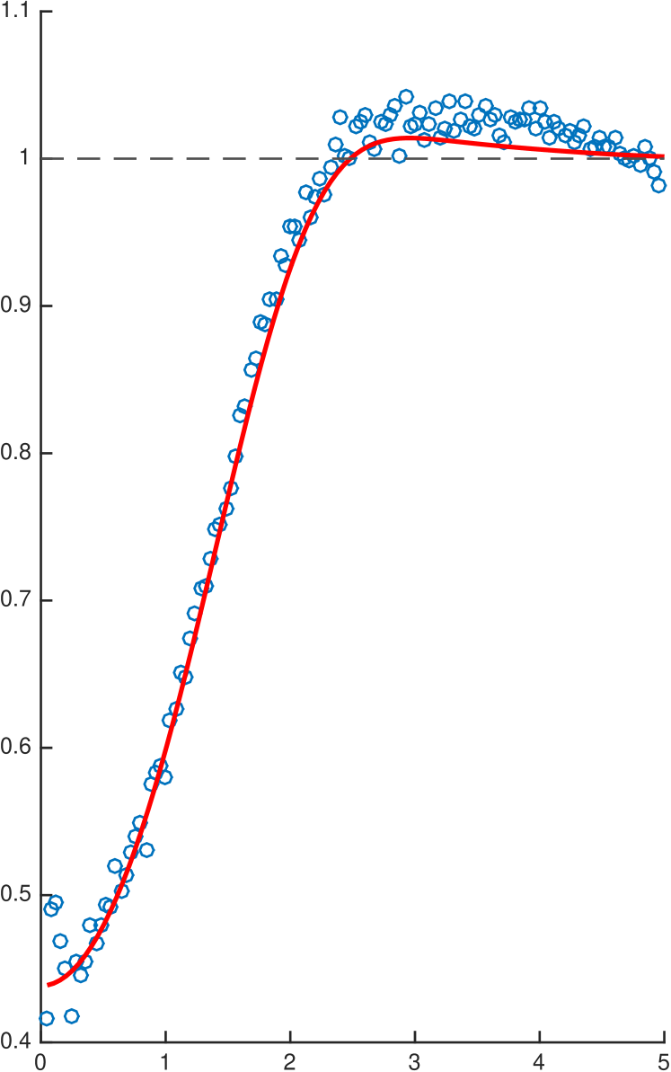
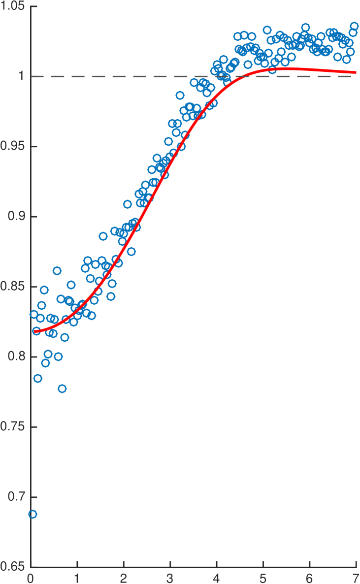
Figure 3. Blue points: values of the $2$-point correlation functions at the energy $z_{0}=1.6$, obtained by numerically computing the spectra of the two operators $P_{h,1}^{\delta}$ (left) and $P_{h,3}$ (right) perturbed by a Gaussian random potential $\delta V_{\omega}$. Red curves: scaling limit $2$-point correlation functions $K^{2,V}_{z_{0}}$ for both operators, as given in (2.30); the horizontal coordinate is the rescaled square distance $|w_{1}-w_{2}|^{2}$.

2.6. Perturbation by random matrix

We now describe the situation where the operator $P_{h}$ is perturbed by a small random matrix $\delta M_{\omega}$, as described in (RM,2.18). In this section we do not need to assume the symmetry property (SYM) for the symbol $p_{0}$. Here as well, we can prove a convergence of the rescaled spectral point process $\mathcal{Z}_{h,z_{0}}^{M}$ (see (2.24)) towards a limiting zero process when $h\to 0$.

2.6.1. Universal limiting point process

Theorem 10.

Let $\Omega\Subset\mathring{\Sigma}$ be as in (2.11). Let $p$ be as in (2.6) satisfying (2.12). Choose $z_{0}\in\Omega$. Then, for any $O\Subset\mathds{C}$ open connected domain, the rescaled spectral point process $\mathcal{Z}_{h,z_{0}}^{M}$ converges in distribution towards the zero point process associated with a random analytic function $\tilde{G}_{z_{0}}$ described below:

$$\mathcal{Z}_{h,z_{0}}^{M}\stackrel{{\scriptstyle d}}{{\longrightarrow}}\mathcal{Z}_{\tilde{G}_{z_{0}}}\text{ on }O\quad\text{ as }h\to 0.$$ (2.33)

The random function $\tilde{G}_{z_{0}}$ is defined as

$$\tilde{G}_{z_{0}}(w)\stackrel{{\scriptstyle\mathrm{def}}}{{=}}\det(g_{z_{0}}^{i,j}(w))_{1\leq i,j\leq J},\quad w\in\mathds{C},$$

where $g_{z_{0}}^{i,j}$, for $1\leq i,j\leq J$, are $J^{2}$ independent GAFs $g_{z_{0}}^{i,j}\sim g_{\sigma^{i,j}_{z_{0}}}$, for the parameters

$$\sigma^{i,j}_{z_{0}}=\frac{1}{2}(\sigma_{+}^{i}(z_{0})+\sigma_{-}^{j}(z_{0}))\,.$$ (2.34)

(we recall that the local classical densities $\sigma_{\pm}^{i}(z_{0})$ associated with the points $\rho_{\pm}^{i}(z_{0})\in p_{0}^{-1}(z_{0})$ are defined in (2.25)).

Theorem 10 tells us that at any given point $z_{0}\in\widetilde{\Omega}\cap\mathring{\Sigma}$ in the bulk of the pseudospectrum, the local rescaled point process of the eigenvalues of $P_{M}^{\delta}$ is given, in the limit $h\to 0$, by the zero process associated with the determinant of a $J\times J$ matrix whose entries are independent GAFs. The GAF situated at the position $i,j$ of the matrix only depends on the portion of the classical spectral densities due to the points $\rho_{+}^{i}(z_{0})$ and $\rho_{-}^{j}(z_{0})$.

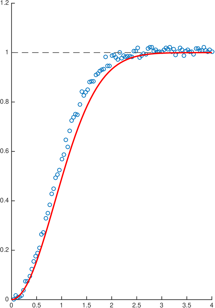
Figure 4. Blue points: values of the $2$-point correlation functions, obtained by numerically computing the spectra of the two operators $P_{h,1}$ (left) and $P_{h,3}$ (right) perturbed by a Gaussian random matrix $\delta M_{\omega}$. The parameters $z_{0},h,\delta$ are as in Figure 3. Red curves: the 2-point correlation function for the Ginibre ensemble, $K^{2,Gin}_{z_{0}}$, as given in (2.37). The horizontal coordinate is the rescaled square distance $|w_{1}-w_{2}|^{2}$.

The rescaled point process $\mathcal{Z}_{h,z_{0}}^{M}$ of the eigenvalues of the perturbed operator $P^{\delta}_{M}$ has a universal limit, which is independent of the specific probability distribution of the potential $M_{\omega}$ (2.16), but only depends on the cardinal $2J$ of the energy shell $p_{0}^{-1}(z)$ the local classical densities $\{\sigma^{j}_{\pm}(z_{0});j=1,\dots,J\}$ (we notice that without the assumption (SYM), the densities $\sigma^{j}_{+}(z_{0})$ and $\sigma^{j}_{-}(z_{0})$ are a priori unrelated).

This limiting process is of a different type from the universal limit of $\mathcal{Z}_{h}^{V}$ studied in the previous section. In particular the function $\tilde{G}_{z_{0}}$ is not given by a simple product of GAFs, but by a more complicated expression, namely a determinant. As we will see below, we conjecture that the zero process of $\tilde{G}_{z_{0}}$ exhibits a quadratic repulsion between the nearby points, as opposed to the zero process of the function $G_{z_{0}}$ in Thm 6.

2.6.2. Scaling limit $k$-point measures

A direct consequence of the convergence of the zero processes $\mathcal{Z}^{M}_{h,z_{0}}$ is the convergence of their $k$-point measures converge to those of the limiting point process.

Corollary 11.

Let $\mu_{h,z_{0}}^{k,M}$ be the $k$-point measure of $\mathcal{Z}_{h,z_{0}}^{M}$, defined as in (2.26), and let $\mu^{k,M}_{z_{0}}$ be the $k$-point measure of the point process $\mathcal{Z}_{\tilde{G}_{z_{0}}}$ described in Thm 10. Then, for any $O\Subset\mathds{C}$ open connected domain and for all $\phi\in\mathcal{C}_{c}(O^{k}\backslash\Delta,\mathds{R}_{+})$,

$$\int_{O^{k}\backslash\Delta}\phi(w)\,\mu_{h,z_{0}}^{k,M}(dw)\longrightarrow\int_{O^{k}\backslash\Delta}\phi(w)\,\mu_{z_{0}}^{k,M}(dw),\quad h\to 0.$$

One can calculate the Lebesgue densities of the limiting $1$-point measures $\mu_{z_{0}}^{1,M}$:

$$d^{1,M}_{z_{0}}(w)=\sum_{i=1}^{J}\frac{\sigma_{+}^{i}(z_{0})+\sigma_{-}^{i}(z_{0})}{2\pi},\quad\forall w\in O.$$ (2.35)

This microscopic density exactly coincides with the macroscopic density of eigenvalues at $z_{0}$ predicted by the probabilistic Weyl’s law in Thm 5, see also (2.25). In the case of an operator $P_{h}$ satisfying the symmetry assumption (SYM), this local density is equal to the one obtained for the operator perturbed by a random potential: for such symmetric symbols, the microscopic densities $d^{1,Q}_{z_{0}}$ therefore cannot distinguish between the type of perturbation imposed on $P_{h}$.

On the opposite, we believe that the $k$-point densities $d^{k,Q}_{z_{0}}$ (equivalently, the $k$-point correlation functions $K^{k,Q}_{z_{0}}$) for $k>1$ should distinguish between the two types of perturbation (still assuming the symmetry (SYM)). Unfortunately, we have not been able, so far, to compute in closed form the Lebesgue densities of the limiting $k$-point measures $d^{k,M}_{z_{0}}$ associated with the random function $\tilde{G}_{z_{0}}$ (the determinant of a matrix of independent GAFs). However, the numerical experiments presented in Figure 4, as well as the Proposition 8, lead us to the following

Conjecture 12.

The $k$-point densities $d^{k,M}_{z_{0}}(w)$ of the zero point process of the random function $\tilde{G}_{z_{0}}$ as in Theorem 10 exhibit a quadratic repulsion at short distance. Namely, for any compact set $O\Subset\mathds{C}$, there exists a constant $C>1$ depending only on $O$ and $k$ such that, for all pairwise distinct points $w_{1},\ldots,w_{k}\in O$,

$$C^{-1}\prod_{i<j}|w_{i}-w_{j}|^{2}\leq d^{k,M}_{z_{0}}(w_{1},\dots,w_{k})\leq C\prod_{i<j}|w_{i}-w_{j}|^{2}.$$

In Figure 4 we compare our experimental values of the $2$-point correlation function with the $2$-point correlation function of a well-known spectral point process on $\mathds{C}$, namely the one for the Ginibre ensemble of random matrices [18]. This ensemble corresponds to the spectra of the random matrices $M_{\omega}$ alone, in the case where their coefficients are Gaussian (see eq. (1.6)), in the limit $h\to 0$, or equivalently the limit or large matrices. It is known since the work of Ginibre [18] that the eigenvalues of these matrices repel each other quadratically at short distance. When the eigenvalues are rescaled such that the mean local density is given by $d^{1}(w)=\sigma/\pi$, the 2-point correlation function takes the simple form

$$K^{2,Gin}_{\sigma}(w_{1},w_{2})=1-\exp(-\sigma|w_{1}-w_{2}|^{2})\,.$$ (2.36)

Hence, for our local density (2.35), the 2-point function we draw on Fig. 4 is

$$K^{2,Gin}_{z_{0}}(w_{1},w_{2})=1-\exp\left[-\frac{1}{2}\big{(}\sum_{i=1}^{J}\sigma_{+}^{i}(z_{0})+\sigma_{-}^{i}(z_{0})\big{)}|w_{1}-w_{2}|^{2}\right].$$ (2.37)

This function is markedly different from the scaling function $\kappa(t^{2})$ corresponding to the zero GAF process (2.29). It seems rather close to the experimental data of Fig. 4, eventhough we observe a deviation for values $|w_{1}-w_{2}|\sim 1$. Is this deviation due to the finite value of $h$ used in the experiment? Or does the deviation persist when $h\to 0$, that is in the correlation function $K^{2,M}_{z_{0}}$? We conjecture that the limiting correlation functions $K^{2,M}_{z_{0}}$ are not strictly equal to the Ginibre function $K^{2,Gin}_{z_{0}}$, but that they are becoming closer and closer to them when the number of quasimodes $J$ gets larger and larger (a property which purely concerns the classical symbol $p_{0}$): in this regime $\tilde{G}_{z_{0}}$ is the determinant of a large matrix of independent GAFs. In any case, computing the $k$-point densities for the process $\mathcal{Z}_{G_{z_{0}}}$ seems to us to be an interesting open problem.

Translation invariance

One easy property of the limiting point processes obtained in Theorems 7 and 10, is that they are homogeneous and isotropic. This property is inherited from the similar invariance of the zero process of a single GAF [28].

Proposition 13.

The limiting point processes $\mathcal{Z}_{G_{z_{0}}}$, resp. $\mathcal{Z}_{\tilde{G}_{z_{0}}}$ obtained in Theorems 7 and 10 are invariant in distribution under the action of the group of translations and rotations on $\mathds{C}$. More precisely, for arbitray $\alpha,\beta\in\mathds{C}$ with $|\alpha|=1$ let us define the plane isometry $\tau(w)=\alpha w+\beta$, $w\in\mathds{C}$.

Then, the zero processes of $G_{z_{0}}$ and $\tilde{G}_{z_{0}}$ satisfy

$$\mathcal{Z}_{G_{z_{0}}}\stackrel{{\scriptstyle d}}{{=}}\mathcal{Z}_{G_{z_{0}}\circ\tau},\quad\text{resp.}\quad\mathcal{Z}_{\tilde{G}_{z_{0}}}\stackrel{{\scriptstyle d}}{{=}}\mathcal{Z}_{\tilde{G}_{z_{0}}\circ\tau}\,.$$

2.7. Outline of the proofs

The proof of the main results is built on two distinct parts. In the first part we will reduce the eigenvalue problem of the perturbed operator $P^{\delta}_{h}$ to studying the zeros of a certain random analytic function. To do this, we will start by constructing quasimodes for the unperturbed operator $P_{h}$ in Section 3, and study their interactions in Section 4. Next we will use these quasimodes in Section 5 to construct a well-posed Grushin problem for the perturbed operator $P^{\delta}$, which will yield an effective description of the eigenvalues of $P^{\delta}$ as the zeros of a random analytic function.

The second part has a more probabilistic flavour. We first provide in Section 6 an overview of the notions and results from the theory of random analytic functions used in this paper. The sections 7 and 8 then use these results to finish the proofs of our main theorems.

3. Quasimodes

The aim of this section is provide the ingredients for a well-posed Grushin problem of the unperturbed operator $P_{h}$, cf. (2.9). Our main objective in this section is the construction of the quasimodes $e^{j}_{\pm}(z_{0})$ for the operator $(P_{h}-z_{0})$ (resp. $(P_{h}-z_{0})^{*}$). For this aim we will first factorize our symbol $p$ into a "nice" form, using semiclassical analysis: this factorized form will allow very explicit expressions of our quasimodes.

3.1. Malgrange preparation theorem

We begin by giving an asymptotic factorization of the symbol $p$, (2.6) in a neighbourhood of each of the points $\rho_{\pm}^{j}=(x^{j}_{\pm},\xi_{\pm}^{j})\in p_{0}^{-1}(z_{0})$, see (HYP). The method presented here is an adaptation of [21].

Proposition 14.

Let $\Omega\Subset\mathds{C}$ be as in (2.11), let $z_{0}\in\Omega$ and let $p(h)\sim\sum_{k\geq 0}h^{k}\,p_{k}$ in $S(\mathds{R}^{2},m)$, satisfying (HYP). Let $j=1,\dots,J$ and let $U_{\pm}^{j}$ be open neighbourhoods of $\rho_{\pm}^{j}(z_{0})$. Then, there exists an open, relatively compact neighbourhood of $z_{0}$, denoted by $W(z_{0})$, open sets $V_{\pm}^{j}\subset U_{\pm}$ containing $\rho_{\pm}^{j}(\overline{W(z_{0})})$, and symbols in $S(V_{\pm}^{j},1)$:

$$q^{\pm,j}(x,\xi,z;h)\sim\sum_{k\geq 0}h^{k}q_{k}^{\pm,j}(x,\xi,z),\quad g^{\pm,j}(x,z;h)\sim\sum_{k\geq 0}h^{k}g_{k}^{\pm,j}(x,z)\,,$$ (3.1)

depending smoothly on $z\in W(z_{0})$, such that for all $z\in W(z_{0})$,

$$\begin{split}p(x,\xi;h)-z\sim q^{+,j}(x,\xi,z;h)\#(\xi+g^{+,j}(x,z;h))\quad\text{ in }S(V_{+}^{j},m),\\ p(x,\xi;h)-z\sim(\xi+g^{-,j}(x,z;h))\#q^{-,j}(x,\xi,z;h)\quad\text{ in }S(V_{-}^{j},m).\end{split}$$ (3.2)

Furthermore, the principal symbols $q_{0}^{\pm,j}(x_{\pm}^{j}(z),\xi_{\pm}^{j}(z),z)\neq 0$ and $g_{0}^{\pm,j}(x_{\pm}^{j}(z),z)=-\xi_{\pm}^{j}(z)$.

We recall that $\#$ indicates the Moyal product, which translates the operator composition to the symbolic level [11, Chapter 7]. For symbols $a_{j}\in S(\mathds{R}^{2},\widetilde{m}_{j})$, for $j=1,2$, then

$$a_{1}^{w}\circ a_{2}^{w}=(a_{1}\#a_{2})^{w}.$$

The Moyal product $\#:S(\mathds{R}^{2},\widetilde{m}_{1})\times S(\mathds{R}^{2},\widetilde{m}_{2})\to S(\mathds{R}^{2},\widetilde{m}_{1}\widetilde{m}_{2})$ is a bilinear and continuous map.

Proof.

We will focus on a single point $\rho^{j}_{+}(z)$, and will omit the $\pm$ and $j$ sub/superscripts in the proof. The case of the points $\rho^{j}_{-}$ can be treated identically.

The condition (HYP) implies that for any $z\in\Omega$ we have that $p(\rho(z))-z=0$ and that $\partial_{\xi}p(\rho(z))\neq 0$. Let $z_{0}\in\Omega$. By the Malgrange preparation theorem [27, Theorem 7.5.6], there exist open neighbourhoods $V\subset U$ of $\rho(z_{0})$ and $W(z_{0})\subset\mathds{C}$ of $z_{0}$, as well as smooth functions $q_{0}\in\mathcal{C}^{\infty}(V\times W(z_{0}))$ and $g_{0}\in\mathcal{C}^{\infty}(\pi_{x}(V)\times W(z_{0}))$, such that

$$p(x,\xi)-z=q_{0}(x,\xi,z)(\xi+g_{0}(x,z)),\quad\text{for all }(x,\xi,z)\in V\times W(z_{0}),$$ (3.3)

and $q_{0}(x(z_{0}),\xi(z_{0}),z_{0})\neq 0$, while $g_{0}(x(z_{0}),z_{0})=-\xi(z_{0})$. We can suppose that $q_{0}(x,\xi,z)\neq 0$ in $V\times W(z_{0})$ by potentially shrinking $V$ and $W(z_{0})$. Up to shrinking $W(z_{0})$ we may also assume that $\rho(W(z_{0}))\subset V$, so that $g_{0}(x(z),z)=-\xi(z)$ for all $z\in W(z_{0})$.

Next, we make the formal Ansatz

$$q(x,\xi,z;h)=\sum_{k\geq 0}h^{k}q_{k}(x,\xi,z),\quad g(x,z;h)=\sum_{k\geq 0}h^{k}g_{k}(x,z),$$

and group together the terms of the Moyal product

$$\left.q(x,\xi,z;h)\#(\xi+g(x,z;h))=\mathrm{e}^{\frac{ih}{2}(D_{\xi}D_{y}-D_{x}D_{\eta})}q(x,\xi,z;h)(\eta+g(y,z;h))\right|_{\begin{subarray}{c}y=x\\ \eta=\xi\end{subarray}}$$

with the same power of $h$. For any $N\geq 1$, equating the coefficient of $h^{N}$ of this asymptotic development with the symbol $p_{N}$, we obtain

$$G_{N}(x,\xi,z)=\frac{q_{N}(x,\xi,z)}{q_{0}(x,\xi,z)}\big{(}\xi+g_{0}(x,z)\big{)}+g_{N}(x,z),$$ (3.4)

where

$$\begin{split}&G_{N}(x,\xi,z)=\frac{1}{q_{0}(x,\xi,z)}\left(p_{N}(x,\xi)-\sum_{l=1}^{N-1}q_{N-l}(x,\xi,z)g_{l}(x,z)\right.\\ &\left.\left.+\sum_{k=0}^{N-1}\Big{(}\frac{i}{2}(D_{\xi}D_{y}-D_{x}D_{\eta})\Big{)}^{N-k}\Big{(}q_{k}(x,\xi,z)\eta+\sum_{r=0}^{k}q_{k-r}(x,\xi,z)g_{r}(y,z)\Big{)}\right)\right|_{\begin{subarray}{c}y=x\\ \eta=\xi\end{subarray}}\end{split}$$ (3.5)

Notice that $G_{N}$ only depends on $q_{k}$, $g_{k}$, for $k<N$, and on $p_{N}$. We can determine the functions $q_{k}$ and $g_{k}$ inductively: since

$$\xi(z)+g_{0}(x(z),z)=0,\quad\partial_{\xi}(\xi+g_{0}(x,z))=1,$$

the Malgrange preparation theorem implies the existence of smooth functions $q_{N}/q_{0}$ and $g_{N}$ in $V\times W(z_{0})$ satisfying (3.4). Iterating the procedure, we obtain functions $q_{k}\in\mathcal{C}^{\infty}(V\times W(z_{0}))$, $g_{k}\in\mathcal{C}^{\infty}(\pi_{x}(V)\times W(z_{0}))$, $k\geq 1$, which allow us to construct full symbols $q(x,\xi,h)$ and $g(x,h)$ by Borel summation, which satisfy (3.1) in $S(V,1)$. ∎

3.2. Almost holomorphic extensions

In general the symbol $p(x,\xi,h)$ is not real analytic in the variables $x,\xi$, so that the functions $q(\rho,z)$ and $g(x,z)$ constructed in Prop. 14 are, a priori, not holomorphic in $z$. Yet, we show below that they are almost holomorphic.

We begin by recalling the notion of an almost holomorphic extension of a smooth function. It has been introduced by Hörmander [26] and Nirenberg [35] in different contexts.

Definition 15.

Let $X\subset\mathds{C}^{n}$ be an open set and let $\Gamma\subset X$ be closed. If $f\in\mathcal{C}^{\infty}(X)$, we say that $f$ is almost holomorphic at $\Gamma$ if $\partial_{\overline{z}}f$ vanishes to infinite order there, i.e. for any $N\in\mathds{N}$ there exists a constant $C_{N}>0$ such that for all $z$ in a small neighbourhood of $\Gamma$ in $X$

$$|\partial_{\overline{z}}f(z)|\leq C_{N}\leavevmode\nobreak\ \mathrm{dist\,}(z,\Gamma)^{N}.$$

In this case we write $\partial_{\overline{z}}f(z)=\mathcal{O}(\mathrm{dist\,}(z,\Gamma)^{\infty})$. If $\Gamma=X\cap\mathds{R}^{n}$ then we simply say that $f$ is almost holomorphic.

If $f,g\in\mathcal{C}^{\infty}(X)$ are almost holomorphic at $\Gamma$ and if $f-g$ vanishes to infinite order there, then we say that that $f$ and $g$ are equivalent at $\Gamma$. If $\Gamma=X\cap\mathds{R}^{n}$, then we simply say that $f$ and $g$ are equivalent and we write $f\sim g$.

Any $f\in\mathcal{C}^{\infty}(X\cap\mathds{R}^{n})$ admits an almost holomorphic extension, uniquely determined up to equivalence, see e.g [26, 33]. Before we continue we recall parts of a technical lemma from [33, Lemma 1.5].

Lemma 16.

Let $\Omega\subset\mathds{R}^{d}$ be an open set and suppose that $u\in\mathcal{C}^{\infty}(\Omega)$. Let $v(x)$ be a Lipschitz continuous function on $\Omega$ so that $|v(x)-v(y)|\leq C_{\Omega^{\prime}}|x-y|$ when $x,y\in\Omega^{\prime}$ and $\Omega^{\prime}\Subset\Omega$. Suppose that for all $N\in\mathds{N}$, we have

$$|u(x)|\leq C_{N,\Omega^{\prime}}|v(x)|^{N},\quad x\in\Omega^{\prime}.$$

Then for all $\Omega^{\prime}\Subset\Omega$, $N\in\mathds{N}$ and any multi-index $\alpha$, there is a constant $C_{N,\Omega^{\prime},\alpha}$ such that

$$|v(x)|^{|\alpha|}\,|D_{x}^{\alpha}u(x)|\leq C_{N,\Omega^{\prime},\alpha}|v(x)|^{N},\quad x\in\Omega^{\prime}.$$

Applying this Lemma to our construction, we will obtain almost holomorphic extensions of the functions $g_{0}(x,z)$ appearing in our construction.

Lemma 17.

Under the hypotheses of Proposition 14, let $\widetilde{g}_{0}^{\pm,j}$ be an almost $x$-holomorphic extension of $g_{0}^{\pm,j}$, for $j=1,\dots,J$. Then, there exists an open relatively compact neighbourhood $W(z_{0})$ of $z_{0}$, open relatively compact sets $X_{\pm}^{j}\subset\mathds{R}$ and small complex neighbourhoods $\widetilde{X}_{\pm}^{j}$ of $X_{\pm}^{j}$ , such that $x_{\pm}^{j}(\overline{W(z_{0})})\subset X_{\pm}^{j}$, and such for any $N\in\mathds{N}$ and any $\alpha,\beta,\gamma\in\mathds{N}$, there exists a constant $C_{N}^{\alpha,\beta,\gamma}>0$ such that for all $z\in W(z_{0})$ and all $x\in\widetilde{X}_{\pm}^{j}$

$$|\partial^{\alpha}_{x}\partial^{\beta}_{z}\partial_{\bar{z}}^{\gamma+1}\widetilde{g}^{\pm,j}_{0}(x,z)|\leq C_{N}^{\alpha,\beta,\gamma}|x-x_{\pm}^{j}(z)|^{N},\qquad\forall z\in W(z_{0}),\quad\forall x\in\widetilde{X}_{\pm}^{j}.$$ (3.6)

Moreover, for any symbol $g_{k}^{\pm,j}$, $k\in\mathds{N}$ (see Proposition 14), for any $\alpha\in\mathds{N}$ and any $N\in\mathds{N}$, there exists a constant $C^{\pm}_{N,\alpha,k,j}>0$ such that

$$|\partial^{\alpha}_{x}\partial_{\bar{z}}\,g^{\pm,j}_{k}(x,z)|\leq C^{\pm}_{N,\alpha,k,j}|x-x_{\pm}^{j}(z)|^{N},\quad x\in X_{\pm}^{j},\ z\in W(z_{0}).$$ (3.7)

Notice in particular that for $x\in X^{j}_{\pm}$ (3.6) reads

$$|\partial_{\bar{z}}g^{\pm,j}_{0}(x,z)|\leq C_{N}|x-x_{\pm}^{j}(z)|^{N}.$$ (3.8)

Proof of Lemma 17.

Again, we focus only on the $+$ case and omit the superscripts $j$ and $+$.

Let $q_{0}(x,\xi,z)\in\mathcal{C}^{\infty}(V\times W(z_{0}))$ and $g_{0}(x,z)\in\mathcal{C}^{\infty}(\pi_{x}(V)\times W(z_{0}))$ be as in Prop. 14, with $V$ an open relatively compact set containing $\rho_{+}(\overline{W(z_{0})})$. As in the proof of that Proposition, we may suppose that $q_{0}(x,\xi,z)\neq 0$ in $V\times W(z_{0})$.

For $\widetilde{V}$ a small relatively compact complex neighbourhood of $V$, let $\widetilde{q}_{0}(x,\xi,z)$ denote an almost $(x,\xi)$-holomorphic extension of $q_{0}(x,\xi,z)$ defined on $\widetilde{V}\times W(z_{0})$, such that

$$\widetilde{q}_{0}(x,\xi,z)\neq 0,\quad(x,\xi,z)\in\widetilde{V}\times W(z_{0}).$$ (3.9)

Similarly, let $\widetilde{g}_{0}(x,z)$, for $x\in\pi_{x}(\widetilde{V})$, denote an almost $x$-holomorphic extension of $g_{0}(x,z)$. Using these two functions, we may extend (3.3) into an almost $(x,\xi)$-holomorphic extension of $p_{0}(x,\xi)-z$, by defining

$$\widetilde{p}_{0}(x,\xi)-z\stackrel{{\scriptstyle\mathrm{def}}}{{=}}\widetilde{q}_{0}(x,\xi,z)(\xi+\widetilde{g}_{0}(x,z)),\quad(x,\xi,z)\in\widetilde{V}\times W(z_{0}).$$ (3.10)

By (HYP), we have that $\partial_{\xi}p_{0}(\rho_{+}(z))\neq 0$ for all $z\in W(z_{0})$. By potentially shrinking $V$, $W(z_{0})$ and $\widetilde{V}$ we can arrange that $\rho_{+}(\overline{W(z_{0})})\subset V$ and that $\partial_{\xi}\widetilde{p}_{0}(x,\xi)\neq 0$ for all $(x,\xi)\in\widetilde{V}$.

Recall from Proposition 14 that $g_{0}(x_{+}(z),z)=-\xi_{+}(z)$ for all $z\in W(z_{0})$. Hence, by potentially shrinking $V$ and $W(z_{0})$ and by restricting $\widetilde{g}_{0}(\cdot,z)$ to an open relatively compact convex complex neighbourhood $\widetilde{X}$ of $X\stackrel{{\scriptstyle\mathrm{def}}}{{=}}\pi_{x}(V)\subset\mathds{R}$, with $\widetilde{X}\Subset\pi_{x}(\widetilde{V})$, we can arrange that $x_{+}(\overline{W(z_{0})})\subset X$ and $(x,-\widetilde{g}(x,z))\in\widetilde{V}$, for all $x\in\widetilde{X}$.

Taking $\xi=-\widetilde{g}_{0}(x,z)$ in (3.10) and then taking the $\partial_{\bar{z}}$ derivative of that equation, we get that for all $x\in\widetilde{X}$ and all $z\in W(z_{0})$,

$$\partial_{\xi}\widetilde{p}_{0}(x,-\widetilde{g}_{0}(x,z))\partial_{\bar{z}}\widetilde{g}_{0}(x,z)+\partial_{\bar{\xi}}\widetilde{p}_{0}(x,-\widetilde{g}_{0}(x,z))\overline{\partial_{z}\widetilde{g}_{0}(x,z)}=0.$$

Since $\widetilde{p}_{0}$ is almost $(x,\xi)$-holomorphic, we have that for any $N\in\mathds{N}$

$$|\partial_{\bar{z}}\widetilde{g}_{0}(x,z)|\leq C_{N}\big{(}\,|\mathrm{Im\,}\widetilde{g}_{0}(x,z)|^{N}+|\mathrm{Im\,}x|^{N}\big{)},\quad x\in\widetilde{X},\ z\in W(z_{0})\,.$$

Since $\mathrm{Im\,}\widetilde{g}_{0}(x_{+}(z),z)=0$, see Proposition 14, and since $\widetilde{g}_{0}$ is a bounded smooth function on $\overline{\widetilde{X}}\times\overline{W(z_{0})}$, it follows by Taylor expansion that

$$|\partial_{\bar{z}}\widetilde{g}_{0}(x,z)|\leq C_{N}^{\prime}|x-x_{+}(z)|^{N},\quad x\in\widetilde{X},\ z\in W(z_{0}).$$ (3.11)

This proves (3.6) in the case $\alpha=\beta=\gamma=0$. Now, observe that, since $(x-x_{+}(z))$ is a smooth function of $(x,z)$, it follows by Lemma 16 that after slightly shrinking $\widetilde{X}$ and $W(z_{0})$, for any $\alpha,\beta,\gamma\in\mathds{N}$,

$$|\partial^{\alpha}_{x}\partial^{\beta}_{z}\partial_{\bar{z}}^{\gamma+1}\widetilde{g}_{0}(x,z)|\leq C_{N}^{\alpha,\beta,\gamma}|x-x_{+}(z)|^{N}.$$ (3.12)

In particular, restricting $x$ to the value $x_{+}(z)\in X_{+}$, that

$$(\partial^{\alpha}_{x}\partial^{\beta}_{z}\partial_{\bar{z}}^{\gamma+1}g_{0})(x_{+}(z),z)=0.$$ (3.13)

Next, using (3.3) and that $g_{0}(x_{+}(z),z)=-\xi_{+}(z)$, see Proposition 14, we obtain by a direct computation of $\{\bar{p}_{0},p_{0}\}(\rho_{+}(z))$ that

$$\mathrm{Im\,}(\partial_{x}g_{0})(x_{+}(z),z)=\frac{\{\bar{p}_{0},p_{0}\}(\rho_{+}(z))}{2i|q_{0}(\rho_{+}(z),z)|^{2}}<0,$$ (3.14)

where the last inequality is a consequence of (HYP). By differentiating (3.10) with respect to $x$ and $\overline{z}$ and by evaluating it at the point $(x_{+}(z),\xi_{+}(z),z)$ we get that

$$(\partial_{\bar{z}}q_{0})(x_{+}(z),\xi_{+}(z),z)=0.$$

By repeated differentiation of (3.10) and induction using the Leibniz rule, we obtain

$$(\partial_{\rho}^{\eta}\partial_{\bar{z}}q_{0})(x_{+}(z),\xi_{+}(z),z)=0,\quad\forall\eta\in\mathds{N}^{2}.$$ (3.15)

Let us now consider the higher order symbols. For $k\geq 0$, taking $q_{k}\in\mathcal{C}^{\infty}(V\times W(z_{0}))$ and $g_{k}\in\mathcal{C}^{\infty}(\pi_{x}(V)\times W(z_{0}))$ as in Prop. 14, with the sets $V$, $W(z_{0})$ as above, let $\widetilde{q}_{k}$ (resp. $\widetilde{g}_{k}$) denote their respective almost $(x,\xi)$-holomorphic (resp. almost $x$-holomorphic) extensions.

Recall (2.6), and let $\widetilde{p}_{N}$ denote an almost $(x,\xi)$-holomorphic extension of $p_{N}$. The almost holomorphic extensions $\widetilde{g}_{k}$, $\widetilde{q}_{k}$ and $\widetilde{p}_{N}$ define an almost $(x,\xi)$-holomorphic extension of $G_{N}$ via (3.5). Set $f=\widetilde{G}_{N}-\frac{\widetilde{q}_{N}}{\widetilde{q}_{0}}(\xi+\widetilde{g}_{0})-\widetilde{g}_{N}$. Since $f$ vanishes at $V$ by (3.4) and since $\partial_{\overline{x}}f$ and $\partial_{\overline{\xi}}f$ vanish to infinite order at $V$, we see by induction and Taylor expansion that all derivatives of $f$ vanish at $V$, hence

$$\widetilde{G}_{N}(x,\xi,z)\sim\frac{\widetilde{q}_{N}(x,\xi,z)}{\widetilde{q}_{0}(x,\xi,z)}(\xi+\widetilde{g}_{0}(x,z))+\widetilde{g}_{N}(x,z),$$ (3.16)

in the sense of equivalence stated in Definition 15.

We are going to prove (3.7) by an induction argument. Suppose that (3.13), (3.15) hold for $g_{k}$, $q_{k}$ for $0\leq k<N$. Then, by (3.5), (3.9), (3.16) we see that for any $\alpha\in\mathds{N}$,

$$0=\partial_{x}^{\alpha}\partial_{\bar{z}}\widetilde{G}_{N}(x,-\widetilde{g}_{0}(x,z),z)\big{|}_{\begin{subarray}{c}x=x_{+}(z)\end{subarray}}=\partial_{x}^{\alpha}\partial_{\bar{z}}\widetilde{g}_{N}(x,z)\big{|}_{\begin{subarray}{c}x=x_{+}(z)\end{subarray}}=(\partial_{x}^{\alpha}\partial_{\bar{z}}g_{N})(x_{+}(z),z).$$ (3.17)

Similarly as for (3.15), we obtain by repeated differentiation of (3.5) and induction that

$$(\partial_{\rho}^{\eta}\partial_{\bar{z}}q_{N})(x_{+}(z),\xi_{+}(z),z)=0,\quad\forall\eta\in\mathds{N}^{2},$$ (3.18)

and we have shown that (3.13), (3.15) hold for $g_{k}$, $q_{k}$ with $0\leq k\leq N$. Since $X_{+}$ and $W(z_{0})$ are relatively compact, a Taylor expansion shows that for any $k\in\mathds{N}$, any $\alpha\in\mathds{N}$ and any $N\in\mathds{N}$ there exists a constant $C_{N,\alpha,k}>0$ such that

$$|\partial^{\alpha}_{x}\partial_{\bar{z}}g_{k}(x,z)|\leq C_{N,\alpha,k}|x-x_{+}(z)|^{N},\quad x\in X_{+},\ z\in W(z_{0}).\qed$$

3.3. Construction of the quasimodes

From now on we will always assume that the symbol $p_{0}$ satisfies the hypothesis (HYP). Using the decomposition given in Proposition 14 we will construct quasimodes for the operators $P_{h}-z$ and $(P_{h}-z)^{*}$, following the WKB method.

Proposition 18 (Quasimodes).

Let $\Omega\Subset\mathds{C}$ be as in (2.11), let $z_{0}\in\Omega$ and let $p(\cdot;h)\in S(\mathds{R}^{2},m)$ be as in (2.6) and satisfy (HYP). Let $W(z_{0})$ and $X_{\pm}^{j}$, $j=1,\dots,J$, be as in Proposition 14. Let $\chi_{\pm}^{j}\in\mathcal{C}^{\infty}_{0}(X_{\pm}^{j},[0,1])$, such that $\chi_{\pm}^{j}\equiv 1$ in a small neighbourhood of $x_{\pm}^{j}(\overline{W(z_{0})})$. Then, there exist functions

$$\begin{split}&e_{\pm}^{j,hol}(x,z;h)=a_{\pm}^{j}(x,z;h)\chi_{\pm}^{j}\mathrm{e}^{\frac{i}{h}\varphi_{\pm}(x,z)},\quad z\in W(z_{0})\\ &\varphi_{\pm}^{j}(x,z)=-\int_{x_{+}^{j}(z_{0})}^{x}g_{0}^{j,+}(y,z)dy,\quad\varphi_{-}^{j}(x,z)=-\int_{x_{-}^{j}(z_{0})}^{x}\overline{g_{0}^{j,-}(y,z)}dy,\end{split}$$ (3.19)

where $g_{0}^{\pm,j}$ are as in Proposition 14, which depend smoothly on $x\in X_{\pm}^{j}$ and $z\in W(z_{0})$, with $a_{\pm}^{j}(x,z;h)\sim(a_{0}^{\pm,j}(x,z)+ha_{1}^{\pm,j}(x,z)+\dots)$ depending smoothly on $x$ and $z$ such that all derivates are uniformly bounded as $h\to 0$.

Moreover, the states $e_{\pm}^{j,hol}$ have the following properties:

1. For all $z\in W(z_{0})$, and any $n\in\mathds{N}$

   $$\begin{split}&(\partial_{x}^{n}\partial_{\bar{z}}a_{+}^{j})(x_{+}^{j}(z),z;h)=\mathcal{O}(|z-z_{0}|^{\infty}+h^{\infty}),\\ &(\partial_{x}^{n}\partial_{z}a_{-}^{j})(x_{-}^{j}(z),z;h)=\mathcal{O}(|z-z_{0}|^{\infty}+h^{\infty})\end{split}$$

2. The $L^{2}$ norms of those states satisfy

   $$\begin{split}&\|e_{\pm}^{j,hol}(z;h)\|=\mathrm{e}^{\frac{1}{h}\Phi_{\pm}^{j}(z;h)},\\ &\Phi_{\pm}^{j}(z;h)=-\mathrm{Im\,}\varphi_{\pm}^{j}(x_{\pm}^{j}(z),z)+h\log\big{(}h^{\frac{1}{4}}A_{\pm}^{j}(z;h)\big{)},\end{split}$$ (3.20)

   with $\mathrm{Im\,}\varphi_{\pm}^{j}(x_{\pm}^{j}(z),z)\leq 0$, with equality iff $z=z_{0}$, and $A_{\pm}^{j}(z;h)\sim A_{0}^{j,\pm}(z)+hA_{1}^{j,\pm}(z)+\dots$ depending smoothly on $z$ such that all derivatives with respect to $z$ and $\bar{z}$ are bounded when $h\to 0$.

3. Normalizing those states,

   $$e_{\pm}^{j}(x,z;h)\stackrel{{\scriptstyle\mathrm{def}}}{{=}}e_{\pm}^{j,hol}(x,z;h)\mathrm{e}^{-\frac{1}{h}\Phi_{\pm}^{j}(z;h)},$$ (3.21)

   then we see that they are $h^{\infty}$-quasimodes:

   $$\|(P_{h}-z)e_{+}^{j}\|=\mathcal{O}(h^{\infty}),\quad\|(P_{h}-z)^{*}e_{-}^{j}\|=\mathcal{O}(h^{\infty}).$$ (3.22)

4. For all $\psi\in\mathcal{C}^{\infty}_{0}(\mathds{R}^{2},[0,1])$, such that $\psi\equiv 1$ near $\rho^{j}_{\pm}$, and any order function $m^{\prime}$,

   $$\|(1-\psi^{w})e_{+}^{j}\|_{H(m^{\prime})}=\mathcal{O}(h^{\infty}),\quad\|(1-\psi^{w})e_{-}^{j}\|_{H(m^{\prime})}=\mathcal{O}(h^{\infty}).$$ (3.23)

For future use, we voluntarily introduced two versions of the quasimodes: the normalized ones $e_{+}^{j}(z;h)$, and the almost holomorphic ones $e_{\pm}^{j,hol}(z;h)$.

Proof of Proposition 18.

We will give the proof of this Proposition only in the "+" case, since the "-" case is similar. To simplify notation, we will suppress the superscript $j$ until further notice. We begin with the following result:

Lemma 19.

Let $\Omega\Subset\mathds{C}$ be as in (2.11), let $z_{0}\in\Omega$ and let $p(\cdot;h)\in S^{2}(\mathds{R}^{2},m)$ be as in (2.6) and satisfy (HYP). Let $W(z_{0})$ and $X_{+}$ with $x_{+}(\overline{W(z_{0})})\subset X_{+}$ be as in Proposition 14. Let $g^{+}(x,z;h)$ be the symbol constructed in Proposition 14.

Then, the equation

$$(hD_{x}+g^{+}(x))f_{+}(x,z;h)=0,\quad(x,z)\in X_{+}\times W(z_{0})\,,$$ (3.24)

admits a solution $f_{+}^{hol}(x,z;h)$ of the form

$$\begin{split}f_{+}^{hol}(x,z;h)&=a_{+}(x,z;h)\,\mathrm{e}^{\frac{i}{h}\varphi_{+}(x,z)},\quad(x,z)\in X_{+}\times W(z_{0})\\ \text{with}\quad\varphi(x)&=-\int_{x_{+}(z_{0})}^{x}g_{0}^{+}(y,z)dy\,.\end{split}$$ (3.25)

The symbol $a_{+}(x,z;h)\sim a_{0}^{+}(x,z)+ha_{1}^{+}(x,z)+\cdots$ depends smoothly on $x$ and $z$, such that all derivates are bounded as $h\to 0$. Moreover, for all $z\in W(z_{0})$ and any $n\in\mathds{N}$,

$$(\partial_{x}^{n}\partial_{\bar{z}}a^{+})(x_{+}(z),z;h)=\mathcal{O}(|z-z_{0}|^{\infty}+h^{\infty}).$$

Proof.

For any $h\in(0,1]$ and $z\in W(z_{0})$, the first order equation (3.24) can be easily solved by the Ansatz

$$f_{+}^{hol}(x,z;h)\stackrel{{\scriptstyle\mathrm{def}}}{{=}}\exp\Big{(}-\frac{i}{h}\int_{x_{0}}^{x}g^{+}(y,z;h)\,dy\Big{)}\,,$$

where we choose to take the reference point $x_{0}=x_{+}(z_{0})$ independent of $z$. Taking into account the expansion (3.1) of the symbol $g^{+}$, its primitive may be expanded as

$$-\int_{x_{0}}^{x}g^{+}(y,z;h)\,dy\sim\varphi^{+}_{0}(x,z)+h\varphi_{1}^{+}(x,z)+\cdots,\qquad\varphi^{+}_{k}(x,z)\stackrel{{\scriptstyle\mathrm{def}}}{{=}}-\int_{x_{0}}^{x}g^{+}_{k}(y,z)\,dy\,.$$

Separating the first term $\varphi_{+}=\varphi^{+}_{0}$ from the subsequent ones, we may write

$$f_{+}^{hol}(x,z;h)=\mathrm{e}^{\frac{i}{h}\varphi_{+}(x,z)}\,a^{+}(x,z)\,,$$

with the symbol $a^{+}(x,z)\in C^{\infty}(X_{+}\times W(z_{0}))$ admitting an expansion

$$a^{+}(h)\sim a_{0}^{+}+ha_{1}^{+}+h^{2}a_{2}^{+}+\cdots\,,$$

where each term $a_{j}^{+}\in\mathcal{C}^{\infty}(X_{+}\times W(z_{0}))$ depends on the functions $\{\varphi^{+}_{k},k=1,\ldots,j+1\}$.

Alternatively, the expansion $\sum h^{j}a^{+}_{j}$ can be constructed order by order through a WKB construction (see e.g. [11]): one solves iteratively the transport equations

$$-i\partial_{x}a^{+}_{n}(x,z)+\sum_{k=0}^{n}g^{+}_{n+1-k}(x,z)a^{+}_{k}(x,z)=0,\quad n\geq 0\,,$$

by the expressions

$$\begin{split}a_{0}^{+}(x,z)&=\mathrm{e}^{-i\int_{x_{0}}^{x}g^{+}_{1}(y,z;h)\,dy}\,,\\ a_{n}^{+}(x,z)&=-i\,a_{0}^{+}(x,z)\int_{x_{0}}^{x}\sum_{k=0}^{n-1}\frac{g^{+}_{n+1-k}a^{+}_{k}}{a_{0}^{+}}\,(y,z)\,dy\,.\end{split}$$ (3.26)

Let us make some remarks about the phase function $\varphi_{+}$. It is the unique solution to the eikonal equation $\partial_{x}\varphi_{+}(x,z)+g_{0}^{+}(x,z)=0$, satisfying the boundary condition $\varphi_{+}(x_{0},z)=0$. By Proposition 14, $\partial_{x}\varphi_{+}(x_{+}(z);z)=\xi_{+}(z)\in\mathds{R}$, therefore $x_{+}(z)$ is a critical point of $\mathrm{Im\,}\varphi_{+}$. Furthermore, by (3.15),

$$\mathrm{Im\,}\partial^{2}_{x}\varphi_{+}(x_{+}(z),z)=-\mathrm{Im\,}(\partial_{x}g_{0}^{+})(x_{+}(z),z)>0,$$ (3.27)

hence $x_{+}(z)$ is a non-degenerate critical point of $\mathrm{Im\,}\varphi(\cdot,z)$. By potentially shrinking $W(z_{0})$ and $X_{+}$, we can arrange that $x_{+}(\overline{W(z_{0})})\subset X_{+}$ and that (3.27) holds for all $x\in X_{+}$, so that $x_{+}(z)$ is the unique critical point of $\mathrm{Im\,}\varphi_{+}(\cdot,z)$ in $X_{+}$.

By repeated differentiation of (3.26) we check by using (3.7) that for all $x\in X_{+}$, all $z\in W(z_{0})$, any $k\in\mathds{N}$ and any $n\in\mathds{N}$

$$(\partial_{x}^{n}\partial_{\bar{z}}a_{k}^{+})(x,z)=\mathcal{O}(|x-x_{+}(z)|^{\infty}+|x_{+}(z_{0})-x_{+}(z)|^{\infty}).$$

By Taylor expansion of $x_{+}(z)$ around $z_{0}$, we obtain at the critical point:

$$(\partial_{x}^{n}\partial_{\bar{z}}a_{k}^{+})(x_{+}(z),z)=\mathcal{O}(|z-z_{0}|^{\infty}).$$

Summing over all the symbols, we obtain for the full symbol:

$$\forall n\in\mathds{N},\ \forall z\in W(z_{0}),\quad(\partial_{x}^{n}\partial_{\bar{z}}a^{+})(x_{+}(z),z;h)=\mathcal{O}(|z-z_{0}|^{\infty}+h^{\infty}).$$

∎

Remark 20.

In the "$-$" case we construct a solution for $(hD_{x}+\overline{g^{-}(x,z)})f_{-}=0$. Hence, the phase function reads $\varphi_{-}(x;z)=-\int_{x_{-}(z_{0})}^{x}\overline{g_{0}^{-}(y,z)}dy$. Moreover, the transport equations depend on $\overline{g_{0}^{-}(y,z)}$, which is almost anti-holomorphic w.r.t. $z$ at the point $(x_{+}(z),z)$. Hence, for any $n\in\mathds{N}$ we obtain $(\partial_{x}^{n}\partial_{z}a^{-})(x_{-}(z),z;h)=\mathcal{O}(|z-z_{0}|^{\infty}+h^{\infty})$.

Let us proceed with the proof of the Proposition. Let $\chi_{+}\in\mathcal{C}^{\infty}_{0}(X_{+},[0,1])$, such that $\chi_{+}\equiv 1$ in a small neighbourhood of $x_{+}(W(z_{0}))$. We define the smooth function

$$e_{+}^{hol}(x,z)\stackrel{{\scriptstyle\mathrm{def}}}{{=}}\chi_{+}(x,z)\,f_{+}^{hol}(x,z;h),\quad(x,z)\in X_{+}\times W(z_{0})\,.$$

Recall from (3.27) and the discussion afterwards, that $x_{+}(z)$ is the unique critical point of $\mathrm{Im\,}\varphi(\cdot,z)$ in $X_{+}$, and that

$$\mathrm{Im\,}\partial^{2}_{x}\varphi(x_{+}(z),z)>0.$$ (3.28)

In particular we see that $\mathrm{Im\,}\varphi(x,z)-\mathrm{Im\,}\varphi(x_{+}(z),z)\geq 0$ for all $x\in X_{+}$, with a strict inequality for $x\neq x_{+}(z)$. Hence, applying the method of stationary phase, we find that

$$\|e_{+}^{hol}\|=h^{1/4}A_{+}(z;h)\,\mathrm{e}^{\frac{1}{h}\Phi_{+,0}(z)}\stackrel{{\scriptstyle\mathrm{def}}}{{=}}\mathrm{e}^{\frac{1}{h}\Phi_{+}(z;h)}$$ (3.29)

where

$$\Phi_{+,0}(z)=-\mathrm{Im\,}\varphi_{+}(x_{+}(z),z),$$

while the symbol $A_{+}(z;h)\sim A_{0}^{+}(z)+hA_{1}^{+}(z)+\dots$ depends smoothly on $z$, and all derivatives in $z,\bar{z}$ are bounded when $h\to 0$. The principal symbol

$$A_{0}^{+}(z)=\left(\frac{\pi|a_{0}^{+}(x_{+}(z),z)|^{2}}{\mathrm{Im\,}\partial^{2}_{x}\varphi_{+}(x_{+}(z),z)}\right)^{1/4}>0.$$ (3.30)

It follows from (3.27) and the property $\varphi^{+}(x_{+}(z_{0}),z)=0$ that $\Phi_{+,0}(z)\geq 0$ for any $z\in W(z_{0})$, with equality precisely when $z=z_{0}$. Hence, for points such that $|z-z_{0}|\geq 1/C$, the norms of the states $e_{+}^{hol}(\bullet,z)$ are exponentially large. Using Lemma 19, we have

$$(hD_{x}+g^{+})\chi_{+}f_{+}^{hol}=[hD_{x},\chi_{+}]f_{+}^{hol}.$$ (3.31)

Using that $x_{+}(z)\notin\mathrm{supp\,}\chi_{+}^{\prime}$ and the fact that $-\mathrm{Im\,}\varphi_{+}(x,z)$ reaches its maximum only at $x=x_{+}(z)$, we get

$$\|[hD_{x},\chi_{+}]f_{+}^{hol}\|=\mathcal{O}(\mathrm{e}^{-1/Ch})\mathrm{e}^{\frac{1}{h}\Phi_{+,0}(z)}\,,$$

which shows that

$$\|(hD_{x}+g^{+}(z))\,e_{+}^{hol}(z)\|=\mathcal{O}(e^{-C/h})\,\|e_{+}^{hol}(z)\|\,.$$

Next, using (3.29), we define the $L^{2}$-normalised state

$$e_{+}(x,z;h)\stackrel{{\scriptstyle\mathrm{def}}}{{=}}e_{+}^{hol}(x,z;h)\,\mathrm{e}^{-\frac{1}{h}\Phi_{+}(z;h)}$$ (3.32)

which is $\mathcal{C}^{\infty}_{0}(X_{+})$, and depends smoothly on $z\in W(z_{0})$. This normalized state enjoys precise microlocalization properties, as shown in the following

Lemma 21.

Under the assumptions of Lemma 19, if we take any order function $\widetilde{m}$, and for an arbitrary $z\in W(z_{0})$, take any cutoff $\psi\in\mathcal{C}^{\infty}_{0}(\mathds{R}^{2},[0,1])$ such that $\psi=1$ near $\rho_{+}(z)$, we have

$$\|(1-\psi)^{w}e_{+}(z;h)\|_{H(\widetilde{m})}=\mathcal{O}(h^{\infty}).$$ (3.33)

This shows that $e_{+}(z;h)$ is microlocalized on the point $\rho_{+}(z)$.

Proof.

We smoothly extend $g_{+}\in\mathcal{C}^{\infty}(X_{+})$ to $\widetilde{g}_{+}$ in $\mathcal{C}^{\infty}(\mathds{R})$, such that $\widetilde{g}_{+}(x,z;h)=-\frac{i}{C}(x-x_{+}(z))$, for $|x|\geq C$, $C>0$, and such that $\xi+\widetilde{g}_{+}\in S(\mathds{R}^{2},\langle\rho\rangle)$ is elliptic outside $\rho_{+}(z)$. This is possible due to (3.27). Thus, the operator $hD_{x}+\widetilde{g}_{+}=(\xi+\widetilde{g}_{+})^{w}$.

Since $\mathrm{supp\,}\chi_{+}\subset X_{+}$, we have that $\widetilde{g}_{+}=g_{+}$ on the support of $e_{+}$ with respect to $x$. Hence, by (3.31), (3.32),

$$(hD_{x}+\widetilde{g}^{+})^{*}(hD_{x}+\widetilde{g}^{+})e_{+}=\eta\,,\\ \eta=\mathrm{e}^{-\frac{1}{h}\Phi_{+}(z;h)}\Big{(}[hD_{x},[hD_{x},\chi_{+}]]f_{+}^{hol}-2i\mathrm{Im\,}\widetilde{g}^{+}[hD_{x},\chi_{+}]f_{+}^{hol}\Big{)}$$ (3.34)

Using that $x_{+}(z)\notin\mathrm{supp\,}\chi_{+}^{\prime}$, as well as (3.28), the norm $\|\eta\|=\mathcal{O}(\mathrm{e}^{-C/h})$.

Let $\widetilde{\chi}\in\mathcal{C}^{\infty}_{0}(\mathds{R}^{2},[0,1])$, $\widetilde{\chi}=1$ near $\rho_{+}(z)$, and define

$$q^{w}=(hD_{x}+\widetilde{g}^{+})^{*}(hD_{x}+\widetilde{g}^{+})+\widetilde{\chi}^{w}.$$ (3.35)

Notice that its symbol

$$q(x,\xi,z;h)=|\xi+\widetilde{g}_{0}^{+}(x,z)|^{2}+\widetilde{\chi}(x,\xi)+\mathcal{O}(h)_{S(\mathds{R}^{2},\langle\rho\rangle^{2})},$$

is elliptic. Hence, for $h>0$ small enough, $q^{w}$ admits a bounded inverse $b^{w}$, $b\in S(\mathds{R}^{2},\langle\rho\rangle^{-2})$. Notice that by (3.34), (3.35),

$$e_{+}=b^{w}\eta+(b\#\widetilde{\chi})^{w}e_{+}.$$

Let $\psi\in\mathcal{C}^{\infty}_{0}(\mathds{R}^{2},[0,1])$, $\psi=1$ near $\mathrm{supp\,}\widetilde{\chi}$, thus for every order function $\widetilde{m}$,

$$(1-\psi)\#b\#\widetilde{\chi}=\mathcal{O}(h^{\infty})_{S(\mathds{R}^{2},\widetilde{m}^{-1})}.$$

Let us consider the term $((1-\psi)\#b)^{w}\eta$. By repeated integration by parts from (3.34), one can show that $\|\eta\|_{H(\widetilde{m})}=\mathcal{O}(\mathrm{e}^{-C/h})$; since $b^{w}$ and $(1-\psi)^{w}$ are bounded on $H(\widetilde{m})$, it follows that $\|((1-\psi)\#b)^{w}\eta\|_{H(\widetilde{m})}=\mathcal{O}(\mathrm{e}^{-C/h})$. Adding the two contributions, we get the announced estimate $\|(1-\psi)^{w}e_{+}\|_{H(\widetilde{m})}=\mathcal{O}(h^{\infty})$. ∎

Combining Proposition 14 with the Lemmata 19-21, we get that for any $\psi\in\mathcal{C}^{\infty}_{0}(\mathds{R}^{2})$, $\psi=1$ near $\rho_{+}(z)$

$$\begin{split}(P_{h}-z)e_{+}&=(P_{h}-z)\psi^{w}e_{+}+(P_{h}-z)(1-\psi)^{w}e_{+}\\ &=(\psi\#q^{+}\#(\xi+g^{+}))^{w}e_{+}+[P_{h},\psi^{w}]e_{+}+\mathcal{O}(h^{\infty})\\ &=\mathcal{O}(h^{\infty}).\end{split}$$ (3.36)

Here the first term in the second line is $\mathcal{O}(h^{\infty})$ by construction of $e_{+}$. The second term is $\mathcal{O}(h^{\infty})$ by Lemma 21, since the support of the symbol of the commutator is (up to an $\mathcal{O}(h^{\infty})$ term) disjoint from a fixed neighbourhood of $\rho_{+}(z)$.

This concludes the proof of Proposition 18 in the "+" case. The "$-$" case can be obtained following the same steps to construct a quasimode for $(P_{h}-z)^{*}$, using the microlocal factorization of this operator into $(q^{-,w})^{*}(hD_{x}+\overline{g^{-}})$ by Proposition 14. ∎

3.4. Quasimodes for symmetric symbols

Let us now assume (SYM), i.e. that the symbol is symmetric:

$$p(x,\xi;h)=p(x,-\xi;h).$$

Then the formal adjoint $(P_{h}-z)^{*}$ satisfies

$$(P_{h}-z)^{*}=\Gamma(P_{h}-z)\Gamma,\quad\Gamma u\stackrel{{\scriptstyle\mathrm{def}}}{{=}}\overline{u}.$$ (3.37)

Moreover, (SYM) implies that if $\rho=(x,\xi)\in p_{0}^{-1}(z)$ with $\{\mathrm{Re\,}p,\mathrm{Im\,}p\}(\rho)<0$, as in (2.11), (HYP), then $(x,-\xi)\in p_{0}^{-1}(z)$ with $\{\mathrm{Re\,}p,\mathrm{Im\,}p\}(x,-\xi)>0$. Thus, the hypotheses (HYP), (HYP-x) write as

$$\begin{split}&p_{0}^{-1}(z)=\{\rho_{\pm}^{j}(z)=(x^{j}_{\pm}(z),\xi^{j}_{\pm}(z))=(x^{j}(z),\pm\xi^{j}(z));j=1,\dots,J\},\text{ with }\\ &\pm\{\mathrm{Re\,}p,\mathrm{Im\,}p\}(\rho_{\pm}^{j}(z))<0,\text{ and }x^{i}\neq x^{j},\text{if}\ i\neq j.\end{split}$$ (3.38)

For $j=1,\dots,J$ let $e_{+}^{j,hol}$, $\chi_{+}^{j}$, $\varphi_{+}^{j}$, $W(z_{0})$, and $\Phi_{+}^{j}$ be as in Proposition 18. Let us define the "-" quasimode as:

$$e_{-}^{j,hol}(z;h)=\Gamma e_{+}^{j,hol}(z;h).$$ (3.39)

It is then clear form Proposition 18 that for all $z\in W(z_{0})$

$$\|e_{-}^{j,hol}(z;h)\|=\mathrm{e}^{\frac{1}{h}\Phi_{+}^{j}(z;h)}.$$ (3.40)

Moreover, by (3.37), (3.22), we see that since

$$e_{-}^{j}(z;h)=e_{-}^{j,hol}(z;h)\,\mathrm{e}^{-\frac{1}{h}\Phi_{+}^{j}(z;h)}=\Gamma e_{+}^{j}(z;h)\,,$$ (3.41)

$e_{-}^{j}(z;h)$ is indeed a quasimode:

$$\|(P_{h}-z)^{*}e_{-}^{j}(z;h)\|=\mathcal{O}(h^{\infty}).$$

Transposing the proof of Proposition 18, we also obtain that for all $\psi\in\mathcal{C}^{\infty}_{0}(\mathds{R}^{2})$, $\psi=1$ near $\rho^{j}_{-}(z)$,

$$\|(1-\psi^{w})e_{-}^{j}(z;h)\|_{H(m^{\prime})}=\mathcal{O}(h^{\infty}),$$ (3.42)

and for all $\psi\in\mathcal{C}^{\infty}_{0}(\mathds{R}^{2},[0,1])$, $\chi=1$ near the point $(x_{-}^{j}(z),2\xi_{-}^{j}(z))$,

$$\|(1-\psi^{w})(e_{-}^{j}(z;h))^{2}\|_{H(m^{\prime})}=\mathcal{O}(h^{\infty}).$$ (3.43)

In the sequel we shall keep that $\pm$-notation to distinguish the quasimodes, even for symmetric symbols (SYM).

3.5. Relation with the symplectic volume

In this section we will study the functions $\Phi_{\pm}^{j}(z;h)$ governing the $L^{2}$ norm of the holomorphic quasimodes (see Prop. 18). We will strongly make use of the almost holomorphicity of Lemma 17. From the expression (3.20), let us write

$$\Phi_{\pm}^{j}(z;h)=\Phi_{\pm,0}^{j}(z)+h\log\big{(}h^{\frac{1}{4}}A{{}_{\pm}}^{j}(z;h)\big{)},\quad\Phi_{\pm,0}^{j}(z)\stackrel{{\scriptstyle\mathrm{def}}}{{=}}-\mathrm{Im\,}\varphi_{\pm}^{j}(x_{\pm}^{j}(z),z).$$ (3.44)

From now on, let us focus on the function $\Phi_{+}^{j}(z;h)$, and omit to indicate the super/subscript ${}_{+}^{j}$ on all quantities.

By (3.27) and the ensuing discussion, $x(z)=x_{+}^{j}(z)$ is the unique minimum of $x\mapsto\mathrm{Im\,}\varphi(x,z)$ on the support of $\chi_{+}^{j}$. Using the equations (3.8), (3.19) and a Taylor expansion of $x(z)$ at $z_{0}$, we easily obtain

$$(\partial_{\bar{z}}\varphi)(x(z),z)=\mathcal{O}(|x(z)-x(z_{0})|^{\infty})=\mathcal{O}(|z-z_{0}|^{\infty}),$$ (3.45)

which leads to

$$\frac{2}{i}\partial_{z}\Phi_{0}^{j}(z)=(\partial_{z}\varphi)(x(z),z)+\mathcal{O}(|z-z_{0}|^{\infty})\,.$$ (3.46)

Next, recall that by Proposition 14 and (3.19), we have

$$\partial_{x}\varphi(x,z)=-g_{0}(x,z),\quad\text{in particular}\quad\partial_{x}\varphi(x(z),z)=\xi(z).$$

Differentiating w.r.t. $z$ and $\bar{z}$, we get

$$(\partial_{xx}^{2}\varphi)(x(z),z)\partial_{z}x(z)+(\partial_{xz}^{2}\varphi)(x(z),z)=\partial_{z}\xi(z)$$ (3.47)

Differentiating w.r.t. $\bar{z}$ and using Lemma 17, we obtain

$$(\partial_{xx}^{2}\varphi)(x(z),z)\partial_{\bar{z}}x(z)+\mathcal{O}(|z-z_{0}|^{\infty})=\partial_{\bar{z}}\xi(z).$$

Eq. (3.45) is a form of almost holomorphy at the point $(x(z_{0}),z_{0})$. Using Eq. (3.13) one finds a natural extension of this property:

$$(\partial^{2}_{z\bar{z}}\varphi)(x(z),z)=\mathcal{O}(|z-z_{0}|^{\infty})\,.$$

Using this expression, we find

$$\partial^{2}_{z\bar{z}}\big{(}\varphi(x(z),z)\big{)}=\partial_{z}\xi(z)\partial_{\bar{z}}x(z)+\xi(z)\partial^{2}_{z\bar{z}}x(z)+\mathcal{O}(|z-z_{0}|^{\infty})\,.$$

Taking the imaginary part of this equation produces

$$\frac{2}{i}\partial^{2}_{z\bar{z}}\Phi_{0}(z)=\partial_{z}\xi(z)\partial_{\bar{z}}x(z)-\partial_{\bar{z}}\xi(z)\partial_{z}x(z)+\mathcal{O}(|z-z_{0}|^{\infty}).$$ (3.48)

We now restore the $+,j$ notations, and write this expression using 2-forms:

$$\begin{split}-d\xi_{+}^{j}\wedge dx_{+}^{j}(z)&=\big{(}\partial_{z}\xi_{+}^{j}(z)\partial_{\bar{z}}x_{+}^{j}(z)-\partial_{\bar{z}}\xi_{+}^{j}(z)\partial_{z}x_{+}^{j}(z)\big{)}\,d\overline{z}\wedge dz\\ &=\left(4\partial^{2}_{z\bar{z}}\Phi_{+,0}^{j}(z)+\mathcal{O}(|z-z_{0}|^{\infty})\right)\frac{d\overline{z}\wedge dz}{2i}.\\ \end{split}$$ (3.49)

This expressions provides the connection between the volume form in phase space $d\xi\wedge dx$, and the volume form in energy space $\frac{d\bar{z}\wedge dz}{2i}$.

One can perform the symmetric computations for the functions $\Phi_{-,0}^{j}(z)$, and obtain

$$\begin{split}d\xi_{-}^{j}\wedge dx_{-}^{j}(z)&=\big{(}\partial_{\bar{z}}\xi_{-}^{j}(z)\partial_{z}x_{-}^{j}(z)-\partial_{z}\xi_{-}^{j}(z)\partial_{\bar{z}}x_{-}^{j}(z)\big{)}\,d\overline{z}\wedge dz\\ &=\left(4\partial^{2}_{z\bar{z}}\Phi_{-,0}^{j}(z)+\mathcal{O}(|z-z_{0}|^{\infty})\right)\frac{d\overline{z}\wedge dz}{2i}\,.\end{split}$$ (3.50)

Let us now express the factor $4\partial^{2}_{z\bar{z}}\Phi_{+,0}^{j}(z)$ in terms of the symbol $p_{0}$. Differentiating the identity $p_{0}(\rho_{\pm}^{j}(z))=z$, cf. (HYP), we obtain the linear system

$$\begin{cases}&\partial_{\xi}p_{0}(\rho_{\pm}^{j})\partial_{z}\xi_{\pm}^{j}+\partial_{x}p_{0}(\rho_{\pm}^{j})\partial_{z}x_{\pm}^{j}=1\\ &\partial_{\xi}\overline{p}_{0}(\rho_{\pm}^{j})\partial_{z}\xi_{\pm}^{j}+\partial_{x}\overline{p}_{0}(\rho_{\pm}^{j})\partial_{z}x_{\pm}^{j}=0,\end{cases}$$

which can be solved by

$$\partial_{z}\xi_{\pm}^{j}(z)=\frac{-\partial_{x}\overline{p}_{0}}{\{\overline{p}_{0},p_{0}\}}(\rho_{\pm}^{j}(z)),\quad\partial_{z}x_{\pm}^{j}(z)=\frac{\partial_{\xi}\overline{p}_{0}}{\{\overline{p}_{0},p_{0}\}}(\rho_{\pm}^{j}(z)).$$

Using the fact that $x_{\pm}^{j}$, $\xi_{\pm}^{j}$ are real, we get by (3.48), and by a similar computation for $\Phi_{-,0}^{j}$, that

$$4\partial^{2}_{z\bar{z}}\Phi_{\pm,0}^{j}(z)=\left(\frac{\mp 1}{\frac{1}{2i}\{\overline{p}_{0},p_{0}\}(\rho^{j}_{\pm}(z))}+\mathcal{O}(|z-z_{0}|^{\infty})\right).$$

It follows from (HYP) that the first term on the RHS is positive, hence that the functions $\Phi_{\pm}^{j}$ are strictly subharmonic near $z_{0}$.

Identifying the Lebesgue measure $L(dz)$ on the energy plane with the volume form $\frac{d\overline{z}\wedge dz}{2i}$, and denoting by $|d\xi\wedge dx|$ the symplectic volume on $T^{*}\mathds{R}$, the expression (3.49) (resp. (3.50)) relates an infinitesimal volume in the energy space, with an infinitesimal volume near the phase space point $\rho^{j}_{+}$ (resp. $\rho^{j}_{-}$). Adding the contributions of all the $2J$ points in $p_{0}^{-1}(z)$, we obtain the following expression for the push-forward of the symplectic volume $|d\xi\wedge dx|$ through the principal symbol $p_{0}$:

$$\begin{split}&(p_{0})_{*}(|d\xi\wedge dx|)=\sum_{j=1}^{J}\big{(}\sigma_{+}^{j}(z)+\sigma_{-}^{j}(z)\big{)}L(dz),\\ &\text{with }\sigma_{\pm}^{j}(z)\stackrel{{\scriptstyle\mathrm{def}}}{{=}}4\partial^{2}_{z\bar{z}}\Phi_{\pm,0}^{j}(z)+\mathcal{O}(|z-z_{0}|^{\infty})\,.\end{split}$$ (3.51)

Observe that in case we assume the symmetry (SYM), we get $\sigma_{+}^{j}(z)=\sigma_{-}^{j}(z)$.

Remark 22.

The error term $\mathcal{O}(|z-z_{0}|^{\infty})$ will be very small in the following, because we will investigate values of $z$ in some $h^{1/2}$-neighbourhood of $z_{0}$.

4. Interaction between the quasimodes

In this section we study the overlaps (scalar products) between nearby quasimodes. In our notations, the $L^{2}$ scalar product $(u|v)$ is linear w.r.t. $u$ and antilinear w.r.t. $v$.

From the assumption (HYP), we may shrink implies that the neighbourhood $W(z_{0})$, (see Proposition 18) to ensure that

$$\rho_{\pm}^{j}(\overline{W(z_{0})})\cap\rho_{\pm}^{k}(\overline{W(z_{0})})=\emptyset\quad\text{for any }j\neq k.$$ (4.1)

Under the further assumption (HYP-x), we may even assume (up to shrinking $W(z_{0})$ that the cutoffs functions $\chi_{\pm}^{j}$ used to construct our quasimodes have disjoint supports:

$$\mathrm{supp\,}\chi_{\pm}^{j}\cap\mathrm{supp\,}\chi_{\pm}^{k}=\emptyset,\quad\text{for any }j\neq k.$$ (4.2)

Thus, from (4.1) and the microlocalization property (3.23), we have for all $z\in W(z_{0})$,

$$(e_{+}^{j}(z)|e_{+}^{k}(z))=\delta_{jk}+\mathcal{O}(h^{\infty}),\quad(e_{-}^{j}(z)|e_{-}^{k}(z))=\delta_{jk}+\mathcal{O}(h^{\infty}),$$ (4.3)

uniformly for all $z\in W(z_{0})$ (here $\delta_{jk}$ denotes the Kronecker symbol).

Similarly, one obtains by (3.23), (4.1) that for all $z,w\in W(z_{0})$

$$(e_{\pm}^{j}(z)|e_{\pm}^{k}(w))=\mathcal{O}(h^{\infty}),\quad\text{for }j\neq k$$ (4.4)

This quasi-orthogonality reflects the fact that for $j\neq k$, the points $\rho_{\pm}^{j}(z)$ and $\rho_{\pm}^{k}(w)$ remain at positive distance from each other, uniformly when $z,w\in W(z_{0})$.

4.1. Overlaps between nearby quasimodes

The scalar product between quasimodes localized on nearby points is given in the following Propositions, which will be crucial for us later. The first one deals with the overlaps between the "+" quasimodes.

Proposition 23.

Let $(e_{+}^{j,hol}(z)_{z\in W(z_{0})}$ be the quasimodes constructed in Proposition 18. Recall the notation $\Phi_{+,0}^{j}(z;h)$ from (3.44). Then, for $|z-w|\leq c$, with $c>0$ sufficiently small,

$$(e_{+}^{j,hol}(z)|e_{+}^{j,hol}(w))=\mathrm{e}^{\frac{2}{h}\Psi^{j}_{+}(z,w;h)}+\mathcal{O}(h^{\infty})\mathrm{e}^{\frac{1}{h}\Phi_{+,0}^{j}(z)+\frac{1}{h}\Phi_{+,0}^{j}(w)}$$ (4.5)

with

$$\Psi^{j}_{+}(z,w;h)=\Psi^{j}_{+,0}(z,w)+\frac{h}{2}\log\big{(}h^{\frac{1}{2}}b^{j}_{+}(z,w;h)\big{)}\,.$$ (4.6)

Here $\Psi^{j}_{+,0}(z,w)$ is almost $z$-holomorphic and almost $w$-antiholomorphic at $\{(z_{0},z_{0})\}$, and $b_{+}^{j}(z,w;h)\sim b^{+,j}_{0}(z,w)+hb^{+,j}_{1}(z,w)+\dots$ is smooth in $z$ and $w$, with any derivative with respect to $z,\bar{z},w,\bar{w}$ uniformly bounded as $h\to 0$. Moreover,

• $\overline{\Psi_{+}^{j}(z,w;h)}=\Psi_{+}^{j}(w,z;h)$,

• $\Psi^{j}_{+,0}(z,z)=\Phi_{+,0}^{j}(z)$,

• $b_{+}^{j}(z,z;h)=A_{+}^{j}(z,h)^{2}$, with $A_{+}^{j}(z,h)$ given in Proposition 18,

• for $|\zeta_{i}|\leq c$, $i=1,2$, $c>0$ sufficiently small, and for any $N\in\mathds{N}$,

  $$\Psi_{+,0}(z_{0}+\zeta_{1},z_{0}+\zeta_{2})=\sum_{|\alpha|\leq N}(\partial^{\alpha_{1}}_{z}\partial^{\alpha_{2}}_{\bar{z}}\Phi_{+,0})(z_{0})\frac{\zeta_{1}^{\alpha_{1}}\overline{\zeta}_{2}^{\alpha_{2}}}{\alpha!}+\mathcal{O}(|\zeta|^{N+1}).$$

The second proposition, symmetric to the previous one, deals with the overlaps between nearby "$-$" quasimodes.

Proposition 24.

Let $(e_{-}^{j,hol}(z)_{z\in W(z_{0})}$ be the quasimodes constructed in Proposition 18. Then, for $|z-w|\leq c$, with $c>0$ sufficiently small,

$$(e_{-}^{j,hol}(z)|e_{-}^{j,hol}(w))=\mathrm{e}^{\frac{2}{h}\Psi^{j}_{-}(z,w;h)}+\mathcal{O}(h^{\infty})\mathrm{e}^{\frac{1}{h}\Phi_{-,0}^{j}(z)+\frac{1}{h}\Phi_{-,0}^{j}(w)},$$ (4.7)

with

$$\Psi^{j}_{-}(z,w;h)=\Psi^{j}_{-,0}(z,w)+\frac{h}{2}\log\big{(}h^{\frac{1}{2}}b^{j}_{-}(z,w;h)\big{)},$$ (4.8)

Here $\Psi^{j}_{-,0}(z,w)$ is almost $z$-antiholomorphic and almost $w$-holomorphic at $\{(z_{0},z_{0})\}$, and $\Phi_{-,0}^{j}(z;h)$ is the function defined in (3.44). The symbol $b_{-}^{j}(z,w;h)\sim b^{-,j}_{0}(z,w)+hb^{-,j}_{1}(z,w)+\dots$ is smooth in $z$ and $w$, with any derivative with respect to $z,\bar{z},w,\bar{w}$ uniformly bounded as $h\to 0$. Moreover,

• $\overline{\Psi_{-}^{j}(z,w;h)}=\Psi_{-}^{j}(w,z;h)$,

• $\Psi^{j}_{-,0}(z,z)=\Phi_{-,0}^{j}(z)$,

• $b_{-}^{j}(z,z;h)=A_{-}^{j}(z,h)^{2}$ with $A_{-}^{j}(z,h)$ as in Proposition 18,

• for $|\zeta_{i}|\leq c$, $i=1,2$, $c>0$ small enough, and for any $N\in\mathds{N}$,

  $$\Psi_{-,0}(z_{0}+\zeta_{1},z_{0}+\zeta_{2})=\sum_{|\alpha|\leq N}(\partial^{\alpha_{1}}_{\bar{z}}\partial^{\alpha_{2}}_{{z}}\Phi_{-,0})(z_{0})\frac{\bar{\zeta}_{1}^{\alpha_{1}}\zeta_{2}^{\alpha_{2}}}{\alpha!}+\mathcal{O}(|\zeta|^{N+1}).$$

Proof of Proposition 23.

Until further notice we will suppress the superscript $j$. By Proposition 18 and (3.44) we have that for $z,w\in W(z_{0})$

$$\begin{split}&(e_{+}^{hol}(z)|e_{+}^{hol}(w))=\mathrm{e}^{\frac{1}{h}\Phi_{+,0}(z)+\frac{1}{h}\Phi_{+,0}(w)}I(z,w),\\ &I(z,w)=\int\chi_{+}(x)\,a_{+}(x,z;h)\,\overline{a_{+}(x,w;h)}\,\mathrm{e}^{\frac{i}{h}\Theta(x,z,w)}dx,\end{split}$$ (4.9)

with

$$\begin{split}\Theta(x,z,w)&=\varphi_{+}(x,z)-\overline{\varphi_{+}(x,w)}+i\Phi_{+,0}(z)+i\Phi_{+,0}(w)\\ &\stackrel{{\scriptstyle\mathrm{def}}}{{=}}2\psi(x,z,w)+i\Phi_{+,0}(z)+i\Phi_{+,0}(w)\end{split}$$ (4.10)

By (3.19), (3.44) and the ensuing discussion, we have that for all $x\in\mathrm{supp\,}\chi_{+}$ and $z,w\in W(z_{0})$

$$\mathrm{Im\,}\Theta(x,z,w)\geq 0,$$ (4.11)

with equality on the submanifold $\{(x_{+}(z),z,z)\}$. Here, we used (3.27) and the discussion afterwards, which implies that

$$\partial_{x}\psi(x_{+}(z),z,z)=0,\quad\mathrm{Im\,}\partial^{2}_{xx}\psi(x_{+}(z),z,z)>0.$$ (4.12)

We have in fact $\mathrm{Im\,}(\partial^{2}_{xx}\psi)(x,z,z)>0$ for all $x\in\mathrm{supp\,}\chi_{+}$. Hence, by the method of stationary phase for complex-valued phase functions [33, Theorem 2.3], we see that for $|z-w|<c$, $c>0$ sufficiently small, the integral $I(z,w)$ can be written as

$$I(z,w)=h^{\frac{1}{2}}b_{+}(z,w;h)\mathrm{e}^{\frac{1}{h}(2\Psi_{+,0}(z,w)-\Phi_{+,0}(z)-\Phi_{+,0}(w))}+\mathcal{O}(h^{\infty}),$$ (4.13)

where $b_{+}(z,w;h)\sim b_{+,0}(z,w)+hb_{+,1}(z,w)+\dots$ is smooth in $z$ and $w$, and all derivatives with respect to $z,\bar{z},w,\bar{w}$ are bounded as $h\to 0$. To compute the "off-diagonal" phase function $\Psi_{+,0}(z,w)$, we extend the function $\psi(\cdot,z,w)$ to an almost holomorphic extension $\widetilde{\psi}(\cdot,z,w)$ defined in a small convex complex neighbourhood $\widetilde{X}$ of $\mathrm{supp\,}\chi_{+}$, such that

$$\partial^{2}_{xx}\widetilde{\psi}(x,z,w)\neq 0,\quad\forall x\in\widetilde{X},\ \forall z,w\in W(z_{0})\,.$$

We can indeed find such a neighbourhood of $\mathrm{supp\,}\chi_{+}$, since $\partial^{2}_{xx}\psi(x,z,z)\neq 0$ for all $x\in\mathrm{supp\,}\chi_{+}$. From (4.10), (3.19), we see that $\widetilde{\psi}$ can be obtained by using an almost $x$-holomorphic extension $\widetilde{g}_{0}^{+}$ of $g_{0}^{+}$ in $\widetilde{X}$, and then defining $\widetilde{\varphi}_{+}(x,z)=-\int_{x_{0}}^{x}\tilde{g}_{0}(y,z)\,dy$ by taking as contour of integration the straight line connecting $x_{0}$ to $x\in\widetilde{X}$. The exact relation $\partial_{x}\varphi_{+}(x,z)=-g_{0}^{+}(x,z)$ is then replaced by the following approximate relations: for any $\alpha,\beta\in\mathds{N}$,

$$\partial^{\alpha}_{z}\partial^{\beta}_{\bar{z}}\partial_{x}\widetilde{\varphi}_{+}(x,z)=-\partial^{\alpha}_{z}\partial^{\beta}_{\bar{z}}\widetilde{g}_{0}^{+}(x,z)+\mathcal{O}_{\alpha,\beta}(|\mathrm{Im\,}x|^{\infty}),\quad z\in W(z_{0}),\ x\in\widetilde{X}\,,$$ (4.14)

with the implied constants uniform w.r.t. $z\in W(z_{0})$.

The extension $\widetilde{\psi}$ can then be defined through

$$\widetilde{\psi}(x,z,w)=\widetilde{\varphi}_{+}(x,z)-\overline{\widetilde{\varphi}_{+}(\bar{x},w)}\,.$$ (4.15)

Now, fixing $z,w\in W(z_{0})$, the function $\widetilde{\psi}(\cdot,z,w)$ admits a unique, nondegenerate critical point $x=x^{c}(z,w)\in\widetilde{X}$, namely a point satisfying

$$\partial_{x}\widetilde{\psi}(x^{c}(z,w),z,w)=0,\quad\partial^{2}_{xx}\widetilde{\psi}(x^{c}(z,w),z,w)\neq 0.$$ (4.16)

In particular, on the diagonal $(z,w)=(z,z)$ on finds that $x^{c}(z,z)=x(z)$ is real valued. The phase function appearing in (4.13) is now defined by

$$\Psi_{+,0}(z,w)=i\widetilde{\psi}(x^{c}(z,w),z,w).$$ (4.17)

Since there is an arbitrariness in the extension $\widetilde{\psi}$ of $\psi$, there is also an arbitrariness in the function $\Psi_{+,0}(z,w)$, especially in the regime $|z-w|\asymp 1$; however, in this regime the first term in (4.13) is exponentially small, and therefore absorbed by the $\mathcal{O}(h^{\infty})$ remainder.

Next, let us check that $x^{c}(z,w)$ is an almost $z$-holomorphic and almost $w$-antiholomorphic function at the diagonal $\{(z,z),\ z\in W(z_{0})\}$. Differentiating the first equation in (4.16) with respect to $z$ and $\bar{z}$, one obtains by (4.15) that

$$\begin{split}&\partial_{z}x^{c}(z,w)=\frac{-(\partial^{2}_{xz}\widetilde{\varphi}_{+})(x^{c}(z,w),z)+\mathcal{O}(|\mathrm{Im\,}x^{c}(z,w)|^{\infty})}{2\partial^{2}_{xx}\widetilde{\psi}(x^{c}(z,w),z,w)},\\ &\partial_{\bar{z}}x^{c}(z,w)=\frac{-(\partial^{2}_{x\bar{z}}\widetilde{\varphi}_{+})(x^{c}(z,w),z)+\mathcal{O}(|\mathrm{Im\,}x^{c}(z,w)|^{\infty})}{2\partial^{2}_{xx}\widetilde{\psi}(x^{c}(z,w),z,w)},\end{split}$$ (4.18)

where we used that $\widetilde{\psi}$ is almost $x$-holomorphic. Similar expressions can be obtained for the $w$ and $\bar{w}$ derivatives of $x^{c}$. Lemma 17 and (4.14) imply that

$$\partial_{x\bar{z}}\widetilde{\varphi}_{+}(x^{c}(z,w),z)=\mathcal{O}(|x^{c}(z,w)-x_{+}(z)|^{\infty}).$$

A similar computation as for (4.18) in the case of (4.12) shows that $(\partial_{z}x^{c})(z,z)=\partial_{z}x_{+}(z)=-(\partial_{\bar{w}}x^{c})(z,z)$. Since $x^{c}$ depends smoothly on $z$ and $w$, and since $x^{c}(z,z)=x_{+}(z)$, it follows by Taylor expansion that $|x^{c}(z,w)-x_{+}(z)|=\mathcal{O}(|z-w|)$ and by (4.16) that

$$\partial_{\bar{z}}x^{c}(z,w)=\mathcal{O}(|z-w|^{\infty}),\quad\partial_{w}x^{c}(z,w)=\mathcal{O}(|z-w|^{\infty}).$$

By (4.17), (4.15) and (3.6) in Lemma 17, we then see that $\Psi_{+,0}(z,w)$ is almost $z$-holomorphic at the point $z=w=z_{0}$:

$$\begin{split}-i\partial_{\bar{z}}\Psi_{+,0}(z,w)&=(\partial_{x}\widetilde{\psi})(x^{c}(z,w),z,w)\partial_{\bar{z}}x^{c}(z,w)+\\ &\quad+(\partial_{\bar{x}}{\widetilde{\psi}})(x^{c}(z,w),z,w)\overline{\partial_{z}x^{c}(z,w)}+\frac{1}{2}\partial_{\bar{z}}\widetilde{\varphi}_{+}(x^{c}(z,w),z)\\ &=\mathcal{O}(|z-w|^{\infty}+|z-z_{0}|^{\infty}).\end{split}$$

By (4.9), (3.20), we have the normalization $I(z,z)=1$. Hence $\Psi_{+,0}(z,z)=\Phi_{+,0}(z)$ and $b_{+}(z,z;h)\sim A_{+}(z;h)^{2}$ in $\mathcal{C}^{\infty}(W(z_{0}))$, with $A_{+}(z;h)$ as in Proposition 18. Thus, by Taylor expansion at $(z_{0},z_{0})$ we get for any $N\in\mathds{N}$ and $|\zeta|\ll 1$

$$\Psi_{+,0}(z_{0}+\zeta_{1},z_{0}+\zeta_{2})=\sum_{|\alpha|\leq N}(\partial^{\alpha_{1}}_{z}\partial^{\alpha_{2}}_{\bar{z}}\Phi_{+,0})(z_{0})\frac{\zeta_{1}^{\alpha_{1}}\overline{\zeta}_{2}^{\alpha_{2}}}{\alpha!}+\mathcal{O}(|\zeta|^{N+1}).$$

In particular

$$2\mathrm{Re\,}\Psi_{+,0}(z,w)-\Phi_{+,0}(z)-\Phi_{+,0}(w)=-\partial^{2}_{z\bar{z}}\Phi_{+,0}(z_{0})|z-w|^{2}+\mathcal{O}((|z-z_{0}|,|w-z_{0}|)^{3}).$$

Finally, (4.15) and (4.17) show that $x^{c}(z,w)=\overline{x^{c}(w,z)}$, and hence that $\Psi_{+,0}(w,z)=\overline{\Psi_{+,0}(z,w)}$, from which we draw that $\Psi_{+,0}(z,w)$ is almost $w$-antiholomorphic at the point $\{z=w=z_{0}\}$.

Actually, setting $\Psi_{+}^{j}(z,w;h)=\Psi_{+,0}^{j}(z,w)+\frac{h}{2}\log\big{(}h^{\frac{1}{2}}b_{+}^{j}(z,w;h)\big{)}$, we directly see by (4.9) and (4.13) that $\overline{\Psi_{+}^{j}(z,w;h)}=\Psi_{+}^{j}(w,z;h)$. ∎

The proof of Proposition 24 is totally symmetric to the one of Proposition 23 we have just given.

4.2. Symmetric symbols

Assume (SYM), the additional symmetry of the symbol $p(x,\xi;h)$, we will also need to compute the interaction between the squares of the quasimodes $e_{-}^{j}$, when considering perturbations by a random potential. The construction of these quasimodes was discussed in Section 3.4.

Notice that by (3.38), (3.43) and the assumption (4.2), we have for all $z,w\in W(z_{0})$

$$((e_{-}^{j}(z))^{2}|(e_{-}^{k}(w))^{2})=0,\quad\text{for }j\neq k.$$ (4.19)

Similarly as in the proof of Proposition 18, one obtains by the method of stationary phase that

$$\begin{split}&\|(e_{-}^{j,hol}(z))^{2}\|=\mathrm{e}^{\frac{1}{h}\Phi^{j}_{s}(z;h)},\\ &\Phi^{j}_{s}(z;h)\stackrel{{\scriptstyle\mathrm{def}}}{{=}}\Phi^{j}_{s,0}(z)+h\log\big{(}h^{\frac{1}{4}}A^{j}_{s}(z;h)\big{)},\quad\Phi^{j}_{s,0}(z)\stackrel{{\scriptstyle\mathrm{def}}}{{=}}2\Phi_{+,0}^{j}(z)\end{split}$$ (4.20)

where $\Phi_{+,0}^{j}(z)$ is as in (3.44) and, in view of (3.38), $x_{+}^{j}=x_{-}^{j}=x^{j}$. We remind that $\Phi_{+,0}^{j}(z)\geq 0$, with equality if and only if $z=z_{0}$, and $A^{j}_{s}(z;h)\sim A_{0}^{j,s}(z)+hA_{1}^{j,s}(z)+\dots$ depends smoothly on $z$ such that all derivatives with respect to $z$ and $\bar{z}$ are bounded when $h\to 0$. Moreover,

$$A_{0}^{j,s}(z)=\left(\frac{\pi|a_{0}^{+}(x_{+}(z);z)|^{4}}{2\mathrm{Im\,}\partial_{xx}^{2}\varphi_{+}(x_{+}(z),z)}\right)^{1/4}>0,$$ (4.21)

where $a_{0}^{+}$ is as in (3.26).

Proposition 25.

Suppose that (SYM) holds and that $W(z_{0})\Subset\mathds{C}$, as in Proposition 18 satisfies (4.1), (4.2). Let $\Phi^{j}_{s}(z;h)$, $z\in W(z_{0})$, be as in (4.20). Then, for $|z-w|\leq c$, with $c>0$ sufficiently small,

$$((e_{-}^{j,hol}(z))^{2}|(e_{-}^{j,hol}(w))^{2})=\mathrm{e}^{\frac{2}{h}\Psi^{j}_{s}(z,w;h)}+\mathcal{O}(h^{\infty})\mathrm{e}^{\frac{1}{h}\Phi^{j}_{s,0}(z)+\frac{1}{h}\Phi^{j}_{s,0}(w)},$$ (4.22)

with

$$\Psi^{j}_{s}(z,w;h)=\Psi^{j}_{s,0}(z,w)+\frac{h}{2}\log\big{(}h^{\frac{1}{2}}b^{j}_{s}(z,w;h)\big{)},$$ (4.23)

where $\Psi^{j}_{s,0}(z,w)$ is almost $z$-antiholomorphic and almost $w$-holomorphic at $\{(z_{0},z_{0})\}$ and $b_{s}^{j}(z,w;h)\sim b^{s,j}_{0}(z,w)+hb^{s,j}_{1}(z,w)+\dots$ is smooth in $z$ and $w$ and all derivatives with respect to $z,\bar{z},w,\bar{w}$ are bounded as $h\to 0$. Moreover,

• $\overline{\Psi_{s}^{j}(z,w;h)}=\Psi_{s}^{j}(w,z;h)$,

• $\Psi^{j}_{s,0}(z,z)=\Phi^{j}_{s,0}(z)=2\Phi_{+,0}^{j}(z)$,

• $b_{s}^{j}(z,z;h)\sim A_{s}^{j}(z,h)^{2}$ with $A_{s}^{j}(z,h)$ as in (4.20),

• for $|\zeta_{i}|\leq c$, $i=1,2$, $c>0$ small enough, and for any $N\in\mathds{N}$,

  $$\Psi_{s,0}^{j}(z_{0}+\zeta_{1},z_{0}+\zeta_{2})=2\sum_{|\alpha|\leq N}(\partial^{\alpha_{1}}_{\bar{z}}\partial^{\alpha_{2}}_{z}\Phi_{+,0})(z_{0})\frac{\overline{\zeta}_{1}^{\alpha_{1}}\zeta_{2}^{\alpha_{2}}}{\alpha!}+\mathcal{O}(|\zeta|^{N+1}).$$

Proof.

Similar to the proof of Proposition 23. ∎

4.3. Finite rank truncation of the quasimodes

In this section we show that the quasimodes $\{e_{\pm}^{j}(z)\}$ essentially live in a finite-dimensional subspace of $L^{2}(\mathds{R})$, which we build using the the orthonormal eigenbasis $\{e_{m}\}_{m\in\mathds{N}}$ of the harmonic oscillator $H=-\partial_{x}^{2}+x^{2}$, corresponding to the eigenvalues $\{\lambda_{m}=2m+1\}$.

For any $N\in\mathds{N}$, let us call $\Pi_{N}$ the orthogonal projector on the subspace of $L^{2}$ spanned by the states $\{e_{m}\}_{0\leq m\leq N}$. In the following Lemma we show that if $N$ is chosen large enough, this projection does essentially not modify our quasimodes.

Lemma 26.

Let $W(z_{0})\Subset\mathds{C}$ be as in Proposition 18, and satisfying (4.2). Let $\{e_{\pm}^{j}(z),z\in W(z_{0})\}$ be the normalized quasimodes constructed in Proposition 18. Then, if $C_{1}>0$ is chosen sufficiently large, taking $N(h)=C_{1}/h^{2}$, we have

$$\forall z\in W(z_{0}),\ \forall j=1,\ldots,J,\quad\|(1-\Pi_{N(h)})\,e_{\pm}^{j}(z)\|=\mathcal{O}(h^{\infty}).$$ (4.24)

In the case of a symmetric symbol (SYM), we will also need the estimate

$$\forall z\in W(z_{0}),\ \forall j=1,\ldots,J,\quad\|(1-\Pi_{N(h)})\,(e_{\pm}^{j}(w))^{2}\|=\mathcal{O}(h^{\infty}).$$ (4.25)

In both cases the $\mathcal{O}(h^{\infty})$ remainder is uniform w.r.t. $z\in W(z_{0})$ and $h\in(0,1]$.

Proof.

We will focus on proving the first estimate, the estimate for squared quasimodes being very similar.

Let $U\Subset\mathds{R}^{2}$ be a bounded open set, so that

$$\bigcup_{j=1}^{J}\rho_{\pm}^{j}\left(\overline{W(z_{0})}\right)\subset U.$$ (4.26)

Our proof will amount to show that the projector $\Pi_{N(h)}$ is microlocally equal to the identity in a neighbourhood of $U$.

Let $\psi\in\mathcal{C}^{\infty}_{c}(\mathds{R}^{2},[0,1])$ such that $\psi\equiv 1$ in a small neighbourhood of $\overline{U}$ and $\mathrm{supp\,}\psi\subset B(0,R)\subset\mathds{R}^{2}$ the ball of radius $R$ centered at $0$, for some sufficiently large $R>0$ . Then, by the microlocalization property (3.23), we have

$$\|(1-\psi^{w})e_{\pm}^{j}(z)\|=\mathcal{O}(h^{\infty}),\quad\text{uniformly in $z\in W(z_{0})$.}$$ (4.27)

It suffices to prove that there exists a constant $C_{1}>0$ such that

$$\forall z\in W(z_{0}),\forall m>N(h)=C_{1}/h^{2},\qquad\|\psi^{w}(x,hD_{x})e_{m}\|=\mathcal{O}(\lambda_{m}^{-\infty})\,,$$ (4.28)

where the implied constant is uniform w.r.t. $m>N(h)$, $h\in(0,1]$ and $z\in W(z_{0})$. Indeed, the above bounds imply that

$$\|(1-\Pi_{N(h)})\psi^{w}e_{\pm}^{i}(z)\|^{2}=\sum_{m>N(h)}|(\psi^{w}e_{\pm}^{i}(z)|e_{m})|^{2}=\mathcal{O}(h^{\infty})\,.$$

Together with (4.27), this shows the requested estimate (4.24).

Let us then prove (4.28). We recall the definition of "exotic" symbol classes. Let $\widetilde{m}$ be an order function as in (2.4). For any and let $0\leq\delta\leq 1/2$, we define a symbol class, generalizing the classes in (2.5):

$$S_{\delta}(\widetilde{m})=S_{\delta}(\mathds{R}^{2},\widetilde{m})\stackrel{{\scriptstyle\mathrm{def}}}{{=}}\{a\in\mathcal{C}^{\infty}(\mathds{R}^{2});\leavevmode\nobreak\ |\partial^{\alpha}_{\rho}a(\rho)|\leq C_{\alpha}h^{-\delta|\alpha|}\widetilde{m}(\rho),\leavevmode\nobreak\ \leavevmode\nobreak\ \forall\rho\in\mathds{R}^{2}\}.$$ (4.29)

For more details on the semiclassical calculus in such a class of symbols we refer the reader to [47, Chapter 4].

For $\lambda>0$, let $U_{\lambda}$ be the unitary transformation on $L^{2}(\mathds{R})$ given by $U_{\lambda}u(x)=\lambda^{1/4}u(\lambda^{1/2}x)$. The harmonic oscillator can be written $H=q^{w}(x,D_{x})$, where $q(x,\xi)=\xi^{2}+x^{2}$. A direct computation shows that

$$U_{\lambda_{m}}(H-\lambda_{m})U_{\lambda_{m}}^{-1}=\lambda_{m}(q^{w}(x,\lambda_{m}^{-1}D_{x})-1)\,,\quad\tilde{h}=\lambda_{m}^{-1}\,.$$ (4.30)

Let us insert the dilation $U_{\lambda_{m}}$ in the expression we want to estimate:

$$\|\psi^{w}(x,hD_{x})e_{m}=\|U_{\lambda_{m}}\psi^{w}(x,hD_{x})U_{\lambda_{m}}^{-1}\,\tilde{e}_{m})\|,\quad\tilde{e}_{m}=U_{\lambda_{m}}e_{m}.$$

We notice that

$$(q^{w}(x,\tilde{h}D_{x})-1)\tilde{e}_{m}=0\,.$$ (4.31)

We want to write $U_{\lambda_{m}}\psi^{w}(x,hD_{x})U_{\lambda_{m}}^{-1}$ as a pseudodifferential operator for the $\tilde{h}$-calculus. An easy computation shows that

$$U_{\lambda_{m}}\psi^{w}(x,hD_{x})U_{\lambda_{m}}^{-1}=\tilde{\chi}^{w}(x,\tilde{h}D_{x}),\quad\text{for the symbol }\tilde{\chi}(x,\xi)=\psi(\lambda_{m}^{1/2}x,\lambda_{m}^{1/2}h\xi)\,.$$

The symbol $\tilde{\chi}$ belongs to the exotic class $\widetilde{S}_{1/2}(1)$, the analogue of $S_{1/2}(1)$ (see (4.29)) for the semiclassical parameter $\tilde{h}$. Our task is thus to show that the norm

$$\|\psi^{w}(x,hD_{x})e_{m}\|=\|\tilde{\chi}^{w}(x,\tilde{h}D_{x})\tilde{e}_{m}\|$$ (4.32)

is very small when $\tilde{h}\to 0$. Since we are in the parameter range $m>N(h)$, we have $\lambda_{m}^{1/2}>\sqrt{2C_{1}}h^{-1}$, hence $\lambda_{m}^{1/2}h>\sqrt{2C_{1}}$. As a result, since $\psi$ was assumed to be supported in some compact neighbourhood of $\bar{U}$, by taking $C_{1}$ large enough we can ensure that $\tilde{\chi}$ is supported inside the ball $B(0,1/3)\subset\mathds{R}^{2}$.

On the other hand, (4.31) implies that the $\tilde{h}$-wavefront set of $\tilde{e}_{m}$ is contained in the unit circle $q^{-1}(1)$. As we show below, these two facts imply that $\tilde{\chi}(x,\tilde{h}D_{x})\tilde{e}_{m}=\mathcal{O}_{L^{2}}(\tilde{h}^{\infty})$.

Let $\eta\in\mathcal{C}^{\infty}_{0}(\mathds{R},[0,1])$ such that $\eta\equiv 1$ on $q(B(0,1/2))=[0,1/4]$, and $\mathrm{supp\,}\eta\subset[-2/3,2/3]$. By the functional calculus for semiclassical pseudodifferential operators [11, Chapter 8],

$$\eta(q^{w}(x,\widetilde{h}D_{x}))=g^{w}(x,\widetilde{h}D_{x}),\qquad\text{for a symbol }g\in S(\langle\rho\rangle^{-\infty})).$$ (4.33)

Here $S(\langle\rho\rangle^{-\infty})$ is the intersection of all symbol classes $S(\langle\rho\rangle^{-n})$, $n\geq 0$. Moreover, for any $\chi_{1}\in C^{\infty}_{c}(B(0,1/2))$, we have

$$g\chi_{1}=1+b,\quad\text{for some }b\in\widetilde{h}^{\infty}S(\langle\rho\rangle^{-\infty}).$$ (4.34)

Next, we recall from [11, Chapter 7] a basic fact about the composition of two pseudo differential operators: Let $a_{j}\in\tilde{S}_{\delta}(\mathds{R}^{2},\widetilde{m}_{j})$, for $j=1,2$, then

$$a_{1}^{w}(x,\widetilde{h}D_{x})\circ a_{2}^{w}(x,\widetilde{h}D_{x})=(a_{1}\#a_{2})^{w}(x,\widetilde{h}D_{x}),$$

where the Moyal product $\#:\tilde{S}_{\delta}(\widetilde{m}_{1})\times\tilde{S}_{\delta}(\widetilde{m}_{2})\to\tilde{S}_{\delta}(\widetilde{m}_{1}\widetilde{m}_{2})$ is bilinear and continuous.

Let us choose the cutoff $\chi_{1}\in\mathcal{C}_{c}^{\infty}(B(0,1/2),[0,1])$ such that $\chi\equiv 1$ on $B(0,5/12)$, and set $\chi_{2}=1-\chi_{1}$. By (4.34),

$$\begin{split}\widetilde{\chi}\#g&=\widetilde{\chi}\#g\chi_{1}+\widetilde{\chi}\#g\chi_{2}\\ &=\widetilde{\chi}\#\chi_{1}+\widetilde{\chi}\#b+\widetilde{\chi}\#g\chi_{2}\\ &=\widetilde{\chi}-\widetilde{\chi}\#\chi_{2}+\widetilde{\chi}\#b+\widetilde{\chi}\#g\chi_{2}.\end{split}$$

Since $\mathrm{dist\,}(\mathrm{supp\,}\chi_{2},\mathrm{supp\,}\widetilde{\chi})\geq 1/12$, it follows [47, Theorem 4.25] that

$$(\widetilde{\chi}\#g\chi_{2})^{w}(x,\widetilde{h}D_{x})=\mathcal{O}_{L^{2}\to L^{2}}(\widetilde{h}^{\infty}),\quad(\widetilde{\chi}\#\chi_{2})^{w}(x,\widetilde{h}D_{x})=\mathcal{O}_{L^{2}\to L^{2}}(\widetilde{h}^{\infty}).$$

The bilinearity of the Moyal product shows that $\widetilde{\chi}\#b\in\widetilde{h}^{\infty}\tilde{S}_{1/2}(\langle\rho\rangle^{-\infty})$, and from the Calderón-Vaillancourt theorem that $(\widetilde{\chi}\#b)^{w}(x,\widetilde{h}D_{x})=\mathcal{O}_{L^{2}\to L^{2}}(\widetilde{h}^{\infty}).$ We have obtained

$$\widetilde{\chi}^{w}(x,\widetilde{h}D_{x})=\widetilde{\chi}^{w}(x,\widetilde{h}D_{x})\#\eta(q^{w}(x,\widetilde{h}D_{x}))+\mathcal{O}_{L^{2}\to L^{2}}(\widetilde{h}^{\infty}).$$

Inserting this identify in (4.32) and using the fact that $\tilde{e}_{m}$ is a normalized null eigenstate of $\eta(q^{w}(x,\tilde{h}D_{x}))$ (since $\eta(1)=0$), we get the required estimate:

$$\|\psi^{w}e_{m}\|=\|\widetilde{\chi}^{w}(x,\widetilde{h}D_{x})\eta(q^{w}(x,\widetilde{h}D_{x}))\tilde{e}_{m}\|+\mathcal{O}(\widetilde{h}^{\infty})=\mathcal{O}(\widetilde{h}^{\infty})=\mathcal{O}(\lambda_{m}^{-\infty}).\qed$$

The following result is not of immediate importance, but will be relevant later on in the text.

Lemma 27.

Let $e_{\pm}^{j,hol}(z)$ be the quasimodes constructed in Proposition 18. Take as before $\{e_{k}\}_{k\in\mathds{N}}$ the orthonormal eigenbasis of the harmonic oscillator $H$, associated with the eigenvalues $\{\lambda_{k}=2k+1\}$. Then,

$$\forall m\geq 0,\qquad|(h^{-1/4}e_{\pm}^{j,hol}(z)|e_{m})|=\mathcal{O}(h^{1/4})\,\lambda_{m}^{-1/6}\,\mathrm{e}^{\frac{1}{h}\Phi_{\pm,0}^{j}(z)}\,,$$ (4.35)

where $\Phi_{\pm,0}^{j}(z)$ is given in (3.44). Similarly, the squared quasimodes satisfy

$$\forall m\geq 0,\qquad|(h^{-1/4}(e_{-}^{j,hol}(z))^{2}|e_{m})|=\mathcal{O}(h^{1/4})\,\lambda_{m}^{-1/6}\,\mathrm{e}^{\frac{2}{h}\Phi_{+,0}^{j}(z)}.$$

In both estimates the implied constant is uniform w.r.to $m\in\mathds{N}$, $h\in(0,1]$ and $z\in W(z_{0})$.

Proof.

We only show the case of the nonsquared quasimodes, the other case being similar. By the Hölder inequality,

$$|(h^{-1/4}e_{\pm}^{j,hol}(z)|e_{m})|\leq\|(h^{-1/4}e_{\pm}^{j,hol}(z)\|_{L^{1}}\,\|e_{m}\|_{L^{\infty}}.$$

Using (3.28), the method of stationary phase yields

$$\|h^{-1/4}e_{\pm}^{j,hol}(z)\|_{L^{1}}=\mathcal{O}(h^{\frac{1}{4}})\,\mathrm{e}^{\frac{1}{h}\Phi_{+,0}^{j}(z)},$$

where $\Phi_{+,0}^{j}(z)$ is as in (3.44). By [31, Corollary 3.2], there exists a constant $C>0$, such that for all $m\in\mathds{N}$,

$$\|e_{m}\|_{\infty}\leq C\lambda_{m}^{-1/6}\|e_{m}\|_{L^{2}}.$$ (4.36)

∎

Remark 28.

The choice of the orthonormal basis $(e_{m})_{m\geq 0}$ used to define the truncation operator is rather arbitrary, as explained in [21, 23]. What is needed is the fact that for $N=N(h)$ large enough, the projection $\Pi_{N(h)}$ on the subspace spanned by a collection of $N(h)$ of those states is microlocally equivalent to the identity in some given bounded region $U\subset\mathds{R}^{2}$. Any orthonormal basis of $L^{2}(\mathds{R})$ will have this property, but the number $N(h)$ of necessary state will depend on the choice of basis.

In [21] the author used the eigenbasis of the semiclassical harmoric oscillator $q^{w}(x,hD_{x})$, in which case it was sufficient to include only $\mathcal{O}(h^{-1})$ eigenstates. Our choice to use the nonsemiclassical harmonic oscillator $H$ requires to include a larger number $N(h)=\mathcal{O}(h^{-2})$ of states. This choice was guided by the extra requirement that each quasimode $e^{j}_{\pm}(z)$ should decomposes into many basis states $e_{m}$ (as shown by Lemma 27), a fact which will be important in Section 7.3 when applying the Central Limit Theorem.

5. Grushin Problem

We begin by giving a short refresher on Grushin problems. They have become an important tool in microlocal analysis and are employed in a vast number of works, especially when dealing with spectral studies of nonselfadjoint operators. As reviewed in [42], the central idea is to analyze the operator $P(z)=(P-z):\mathcal{H}_{1}\to\mathcal{H}_{2}$ by extending this operator into a larger operator of the form

$$\begin{pmatrix}P(z)&R_{-}\\ R_{+}&0\\ \end{pmatrix}:\mathcal{H}_{1}\oplus\mathcal{H}_{-}\longrightarrow\mathcal{H}_{2}\oplus\mathcal{H}_{+},$$

where $\mathcal{H}_{\pm}$ (resp. $R_{\pm}$) are well-chosen auxiliary spaces (resp. operators). The Grushin problem is said to be well-posed if this matrix of operators is bijective for the range of $z$ under study, with a good control on its inverse. In the cases where $\dim\mathcal{H}_{-}=\dim\mathcal{H}_{+}<\infty$, on writes this inverse blockwise as

$$\begin{pmatrix}P(z)&R_{-}\\ R_{+}&0\\ \end{pmatrix}^{-1}=\begin{pmatrix}E(z)&E_{+}(z)\\ E_{-}(z)&E_{-+}(z)\\ \end{pmatrix}.$$

The key observation, going back to Schur’s complement formula or, equivalently, the Lyapunov-Schmidt bifurcation method, is the following: the operator $P(z):\mathcal{H}_{1}\rightarrow\mathcal{H}_{2}$ is invertible if and only if the finite rank operator $E_{-+}(z):\mathcal{H}_{+}\to\mathcal{H}_{-}$ is invertible, in which case both inverses are related by:

$$P(z)^{-1}=E(z)-E_{+}(z)E_{-+}^{-1}(z)E_{-}(z).$$

The finite rank operator $E_{-+}(z)$ is often called an effective Hamiltonian for the original problem $P(z)$. As opposed to $P(z)$, it depends in a nonlinear way of the variable $z$, but it has the advantage to be finite dimensional. In a sense, $E_{-+}(z)$ encapsulates, in a compact way, the spectral properties of $P$.

5.1. Grushin problem for our unperturbed nonselfadjoint operator

Hager [21] showed how to construct an efficient Grushin problem for our nonselfadjoint operator $P_{h}$, using the quasimodes constructed in Proposition 18.

Proposition 29 (Unperturbed Grushin).

Let $p(\cdot;h)$ in $S(\mathds{R}^{2},m)$ be as in (2.6) and satisfy (2.8), (HYP). Let $W(z_{0})\Subset\mathds{C}$ and $\{e_{\pm}^{j}(z),z\in W(z_{0})\}$, $j=1,\dots,J$, be as in Proposition 18, with $W(z_{0})$ satisfying (4.1).

For $z\in W(z_{0})$ let

$$\mathcal{P}(z)=\begin{pmatrix}P_{h}-z&R_{-}(z)\\ R_{+}(z)&0\\ \end{pmatrix}:H(m)\times\mathds{C}^{J}\longrightarrow L^{2}\times\mathds{C}^{J}\,,$$

with

$$(R_{+}(z)u)_{j}\stackrel{{\scriptstyle\mathrm{def}}}{{=}}(u|e_{+}^{j}(z)),\ \ u\in H(m),\qquad R_{-}(z)u_{-}\stackrel{{\scriptstyle\mathrm{def}}}{{=}}\sum_{j=1}^{J}u_{-}^{j}e_{-}^{j}(z),\leavevmode\nobreak\ \leavevmode\nobreak\ u_{-}\in\mathds{C}^{J}.$$ (5.1)

Then, $\mathcal{P}(z)$ is bijective, with bounded inverse:

$$\mathcal{E}(z)=\begin{pmatrix}E(z)&E_{+}(z)\\ E_{-}(z)&E_{-+}(z)\\ \end{pmatrix}:L^{2}\times\mathds{C}^{J}\longrightarrow H(m)\times\mathds{C}^{J}.$$

The components $E_{\pm}(z)$ are given by

$$(E_{-}(z)v)_{j}=(v|e_{-}^{j}(z))+\mathcal{O}(h^{\infty}),\leavevmode\nobreak\ \leavevmode\nobreak\ v\in L^{2},\qquad E_{+}(z)v_{+}=\sum_{j=1}^{J}v_{+}^{j}e_{+}^{j}(z)+\mathcal{O}(h^{\infty}),\leavevmode\nobreak\ \leavevmode\nobreak\ v_{+}\in\mathds{C}^{J}\,.$$ (5.2)

Finally, the blocks of $\mathcal{E}(z)$ admit the following bounds in the semiclassical limit:

$$\begin{split}\|E(z)\|_{L^{2}\to H(m)}=\mathcal{O}(h^{-1/2}),&\quad\|E_{+}(z)\|_{\mathds{C}^{J}\to L^{2}}=\mathcal{O}(1),\\ \|E(z)\|_{L^{2}\to\mathds{C}^{J}}=\mathcal{O}(1),&\quad\|E_{-+}(z)\|_{\mathds{C}^{J}\to\mathds{C}^{J}}=\mathcal{O}(h^{\infty}),\end{split}$$

uniformly for $z\in W(z_{0})$.

Proof.

One can follow line by line, with the obvious changes, the proof of [21, Proposition 4.1]. ∎

5.2. Grushin problem for the perturbed operator

We wish to study the eigenvalues of

$$P^{\delta}=P_{h}+\delta Q,$$ (5.3)

where $\delta>0$ satisfies (1.7) and $Q$ is given by a random matrix $M_{\omega}$, as in (2.18), or by a random potential $V_{\omega}$, as in (2.19). Recall from (2.20) that we have restricted the random variables used to construct $M_{\omega}$ and $V_{\omega}$, to large discs of radius $C/h$. By the tail estimate (2.17) and by the fact that $N(h)=C_{1}/h^{2}$, this restriction holds with probability close to one, more precisely there exists a constant $C_{2}>0$ such that

$$\begin{split}&\mathds{P}\big{[}|q_{i,j}|\leq C/h,\leavevmode\nobreak\ \forall i,j<N(h)\big{]}\geq 1-\kappa N(h)^{2}h^{4+\varepsilon_{0}}=1-C_{2}h^{\varepsilon_{0}},\\ &\mathds{P}\big{[}|v_{i}|\leq C/h,\leavevmode\nobreak\ \forall i<N(h)\big{]}\geq 1-\kappa N(h)h^{4+\varepsilon_{0}}=1-C_{2}h^{2+\varepsilon_{0}}.\end{split}$$ (5.4)

Thus, by (5.4), we have with probability $\geq 1-C_{2}h^{\varepsilon_{0}}$, that

$$\|M_{\omega}\|_{HS}=N(h)^{-1}\Big{(}\sum_{i,j<N(h)}|q_{i,j}|^{2}\Big{)}^{1/2}\leq Ch^{-1}.$$ (5.5)

Similarly, using (5.4), (4.36), we have with probability $\geq 1-C_{2}h^{2+\varepsilon_{0}}$, for $h$ small enough,

$$\|V_{\omega}\|_{\infty}\leq N(h)^{-1}\sum_{n<N(h)}|v_{n}|\|e_{n}\|_{\infty}\leq Ch^{-1}.$$ (5.6)

This proves the estimates (2.21) and (2.22) on the size of the perturbations.

Until further notice we will work in the restricted probability space, where all $|q_{i,j}|\leq C/h$ respectively $|v_{j}|\leq C/h$. Then, (5.5) respectively (5.6) holds. Using Proposition 29, we obtain a well-posed Grushin Problem for the perturbed operator $P^{\delta}$.

Proposition 30 (Pertubed Grushin).

Let $p(\cdot;h)$ in $S(\mathds{R}^{2},m)$ be as in (2.6) and satisfy (2.8), (HYP). Let $P^{\delta}$ be as in (5.3) with $\delta>0$ satisfying (1.7). For $z\in W(z_{0})$ let

$$\mathcal{P}^{\delta}(z)=\begin{pmatrix}P^{\delta}-z&R_{-}(z)\\ R_{+}(z)&0\\ \end{pmatrix}:H(m)\times\mathds{C}^{J}\longrightarrow L^{2}\times\mathds{C}^{J}$$

with

$$(R_{+}(z)u)_{j}\stackrel{{\scriptstyle\mathrm{def}}}{{=}}(u|e_{+}^{j}(z)),\leavevmode\nobreak\ \leavevmode\nobreak\ u\in H(m),\qquad R_{-}(z)u_{-}\stackrel{{\scriptstyle\mathrm{def}}}{{=}}\sum_{j=1}^{J}u_{-}^{j}e_{-}^{j}(z),\leavevmode\nobreak\ \leavevmode\nobreak\ u_{-}\in\mathds{C}^{J}.$$ (5.7)

Then, $P^{\delta}(z)$ is bijective with bounded inverse

$$\mathcal{E}^{\delta}(z)=\begin{pmatrix}E^{\delta}(z)&E_{+}^{\delta}(z)\\ E_{-}^{\delta}(z)&E_{-+}^{\delta}(z)\\ \end{pmatrix}:L^{2}\times\mathds{C}^{J}\longrightarrow H(m)\times\mathds{C}^{J},$$

such that $\mathcal{P}^{\delta}\mathcal{E}^{\delta}=1_{L^{2}\times\mathds{C}^{J}}$ and $\mathcal{E}^{\delta}\mathcal{P}^{\delta}=1_{H(m)\times\mathds{C}^{J}}$.

Moreover, the perturbed blocks $E^{\delta}_{\pm}$, $E^{\delta}_{-+}$ are related as follows with the unperturbed blocks of Proposition 29:

$$E^{\delta}_{-}=E_{-}+\mathcal{O}(\delta h^{-3/2}),\quad E^{\delta}_{+}=E_{+}+\mathcal{O}(\delta h^{-3/2}),$$ (5.8)

and

$$E^{\delta}_{-+}=E_{-+}-\delta E_{-}QE_{+}+\mathcal{O}(\delta^{2}h^{-5/2}).$$ (5.9)

Proof.

The result follows from an application of the Neumann series. Let $\mathcal{E}$ be as in Proposition 29, then

$$\mathcal{P}^{\delta}\mathcal{E}=\mathcal{P}\mathcal{E}+\begin{pmatrix}\delta Q&0\\ 0&0\\ \end{pmatrix}\mathcal{E}=1+\begin{pmatrix}\delta QE&\delta QE_{+}\\ 0&0\\ \end{pmatrix}=1+K.$$

By Proposition 29 and (5.5), (1.7), $\|K\|\leq\delta\|Q\|\|E\|=\mathcal{O}(\delta h^{-3/2})\ll 1$. Thus, $\mathcal{P}^{\delta}$ has the inverse $\mathcal{E}(1+K)^{-1}$ and, by a Neumann series expansion, we get

$$\begin{split}\mathcal{E}^{\delta}&=\begin{pmatrix}E^{\delta}(z)&E_{+}^{\delta}(z)\\ E_{-}^{\delta}(z)&E_{-+}^{\delta}(z)\\ \end{pmatrix}\\ &=\begin{pmatrix}\sum_{n=0}^{\infty}(-1)^{n}E(\delta QE)^{n}&\sum_{n=0}^{\infty}(-1)^{n}(\delta QE)^{n}E_{+}\\ &\\ \sum_{n=0}^{\infty}(-1)^{n}E_{-}(\delta QE)^{n}&E_{-+}+\delta\sum_{n=1}^{\infty}(-1)^{n}E_{-}(\delta QE)^{n-1}QE_{+}\\ \end{pmatrix}.\end{split}$$ (5.10)

This, yields the claimed estimates and concludes the proof. ∎

Using Propositions 18, 29 and (5.9), we get

$$(E_{-+}^{\delta}(z))_{i,j}=-\delta(Qe_{+}^{j}|e_{-}^{i})+\mathcal{O}(\delta h^{\infty})+\mathcal{O}(h^{\infty})+\mathcal{O}(\delta^{2}h^{-5/2}).$$ (5.11)

Remark 31.

We will show below that, with high probability, the first term in the right hand side of (5.11) dominates the following ones: the matrix $E_{-+}^{\delta}$ is thus dominated by the perturbation term, eventhough the latter has a small norm. This effect comes from the fact that unperturbed matrix $E_{-+}$ is extremely small, a consequence of the strong pseudospectral effect.

Using the assumption (1.7) on the size of $\delta$ and taking the determinant, we get

$$\det\left[\delta^{-1}E_{-+}^{\delta}(z)\right]=(-1)^{J}\det\left[(Qe_{+}^{j}(z)|e_{-}^{i}(z))_{i,j\leq J}+\mathcal{O}(\delta h^{-5/2})\right].$$ (5.12)

Notice that $\det E_{-+}^{\delta}(z)$ depends smoothly on $z\in W(z_{0})$ since we have used the normalised quasimodes. However, we can make it holomorphic in $z$ since it satisfies a $\overline{\partial}$-equation in $z$. To see this, we take the derivative with respect to $\bar{z}$ of $\mathcal{P}^{\delta}\mathcal{E}^{\delta}=1_{L^{2}\times\mathds{C}^{J}}$, and we get

$$\partial_{\bar{z}}\mathcal{E}^{\delta}=-\mathcal{E}^{\delta}\partial_{\bar{z}}\mathcal{P}^{\delta}\mathcal{E}^{\delta}.$$

Hence,

$$\partial_{\bar{z}}{E}_{-+}^{\delta}=-{E}_{-+}^{\delta}(\partial_{\bar{z}}R_{+})E_{+}^{\delta}-E_{-}^{\delta}(\partial_{\bar{z}}R_{-}){E}_{-+}^{\delta}.$$

This, together with the identity $\partial_{\bar{z}}\log\det{E}_{-+}^{\delta}=\mathrm{tr\,}({E}_{-+}^{\delta})^{-1}\partial_{\bar{z}}{E}_{-+}^{\delta}$ then yields

$$\begin{split}\partial_{\bar{z}}\det{E}_{-+}^{\delta}&=-\mathrm{tr\,}[(\partial_{\bar{z}}R_{+})E_{+}^{\delta}+E_{-}^{\delta}(\partial_{\bar{z}}R_{-})]\det{E}_{-+}^{\delta}\\ &\stackrel{{\scriptstyle\mathrm{def}}}{{=}}-k^{\delta}\det{E}_{-+}^{\delta}\,.\end{split}$$ (5.13)

Let us study the factor $k^{\delta}(z)$. Using the expressions (5.1), (5.2), (5.8), we find

$$\big{(}(\partial_{\bar{z}}R_{+})E_{+}^{\delta}\big{)}_{jj}=(e_{+}^{j}(z)+\mathcal{O}(\delta h^{-3/2})|\partial_{z}e_{+}^{j}(z)),\quad\big{(}E_{-}^{\delta}\partial_{\bar{z}}R_{-})\big{)}_{jj}=(\partial_{\bar{z}}e_{-}^{j}(z)|e_{-}^{j}(z)+\mathcal{O}(\delta h^{-3/2})).$$

The expressions for the quasimodes in Prop. 18 show that $\|\partial_{z}e_{+}^{j}(z)\|=\mathcal{O}(h^{-1})$, $\|\partial_{\bar{z}}e_{-}^{j}(z)\|=\mathcal{O}(h^{-1})$. For instance,

$$\partial_{z}e_{+}^{j}=\mathrm{e}^{-\frac{1}{h}\Phi_{+}^{j}}\Big{(}\partial_{z}e_{+}^{j,hol}-h^{-1}(\partial_{z}\Phi_{+}^{j})e_{+}^{j,hol}\Big{)}=\mathcal{O}(h^{-1})_{L^{2}}.$$ (5.14)

so we have

$$k^{\delta}=\sum_{j=1}^{J}[(e_{+}^{j}|\partial_{z}e_{+}^{j})+(\partial_{\bar{z}}e_{-}^{j}|e_{-}^{j})]+\mathcal{O}(\delta h^{-5/2}),$$ (5.15)

uniformly in $z\in W(z_{0})$. Taking the $\partial_{z}$ derivative of $\|e_{+}^{j,hol}\|=\mathrm{e}^{\Phi_{+}^{j}/h}$, cf. (3.20), we get

$$h^{-1}\partial_{z}\Phi_{+}^{j}=\frac{1}{2}\mathrm{e}^{-\frac{2}{h}\Phi_{+}^{j}}\left((\partial_{z}e_{+}^{j,hol}|e_{+}^{j,hol})+(e_{+}^{j,hol}|\partial_{\bar{z}}e_{+}^{j,hol})\right).$$

Using these identities together with (3.20) and (5.14), we find

$$\begin{split}(e_{+}^{j}|\partial_{z}e_{+}^{j})&=\frac{1}{2}\mathrm{e}^{-\frac{2}{h}\Phi_{+}^{j}}(e_{+}^{j,hol}|\partial_{z}e_{+}^{j,hol})+\mathcal{O}(h^{-1}|z-z_{0}|^{\infty}+h^{\infty})\\ &=h^{-1}\partial_{\bar{z}}\Phi_{+}^{j}+\mathcal{O}(h^{-1}|z-z_{0}|^{\infty}+h^{\infty}).\end{split}$$ (5.16)

Similar computations show that

$$\begin{split}(\partial_{\bar{z}}e_{-}^{j}|e_{-}^{j})&=\frac{1}{2}\mathrm{e}^{-\frac{2}{h}\Phi_{-}^{j}}(\partial_{\bar{z}}e_{-}^{j,hol}|e_{-}^{j,hol})+\mathcal{O}(h^{-1}|z-z_{0}|^{\infty}+h^{\infty})\\ &=h^{-1}\partial_{\bar{z}}\Phi_{-}^{j}+\mathcal{O}(h^{-1}|z-z_{0}|^{\infty}+h^{\infty}),\end{split}$$ (5.17)

which finally results in

$$k^{\delta}=h^{-1}\sum_{j=1}^{J}\big{(}\partial_{\bar{z}}\Phi_{+}^{j}(z)+\partial_{\bar{z}}\Phi_{-}^{j}(z)\big{)}+\mathcal{O}(h^{-1}|z-z_{0}|^{\infty}+\delta h^{-5/2}).$$

Since $k^{\delta}(z)$ depends smoothly on $z\in W(z_{0})$, the equation $\partial_{\bar{z}}l^{\delta}=hk^{\delta}$ can be solved in $W(z_{0})$ (see e.g. [25, Theorem 1.4.4] or [20, page 6]) with a solution of the form

$$l^{\delta}(z)=-2Jh\log(h^{1/4})+\sum_{j=1}^{J}\big{(}\Phi_{+}^{j}(z;h)+\Phi_{-}^{j}(z;h)\big{)}+\mathcal{O}(|z-z_{0}|^{\infty}+\delta h^{-3/2}).$$ (5.18)

Here we added the constant term $-2Jh\log(h^{1/4})$ in order to balance the behaviour of $\Phi_{\pm}^{j}(z_{0};h)=h\log(h^{1/4})+\mathcal{O}(1)$. From (5.13), we conclude that the following function is holomorphic in $z\in W(z_{0})$:

$$\begin{split}G^{\delta}(z;h)&\stackrel{{\scriptstyle\mathrm{def}}}{{=}}(-\delta)^{-J}\mathrm{e}^{\frac{1}{h}l^{\delta}(z)}\det E_{-+}^{\delta}(z)\\ &=\mathrm{e}^{\frac{1}{h}l^{\delta}(z)}\det\left[(Qe_{+}^{j}(z)|e_{-}^{i}(z))_{i,j\leq J}+\mathcal{O}(\delta h^{-5/2})\right].\end{split}$$

Using (5.18) and (3.21), this holomorphic function can be written as

$$\begin{split}G^{\delta}(z;h)=\big{(}1+R_{1}\big{)}\det\left[(Qh^{-1/4}e_{+}^{j,hol}(z)|h^{-1/4}e_{-}^{i,hol}(z))_{i,j\leq J}+R_{2}\right],\end{split}$$ (5.19)

where (using (3.20))

$$\begin{split}&R_{1}\stackrel{{\scriptstyle\mathrm{def}}}{{=}}R_{1}(z;h)=\mathcal{O}(|z-z_{0}|^{\infty}+\delta h^{-3/2}),\\ &R_{2}\stackrel{{\scriptstyle\mathrm{def}}}{{=}}R_{2}(z;h)\stackrel{{\scriptstyle\mathrm{def}}}{{=}}\Lambda_{+}\mathcal{O}(\delta h^{-3})\Lambda_{-},\end{split}$$ (5.20)

where $\Lambda_{\pm}\stackrel{{\scriptstyle\mathrm{def}}}{{=}}\mathrm{diag}(\mathrm{e}^{\frac{1}{h}(\Phi_{\pm}^{j}(z)+\mathcal{O}(|z-z_{0}|^{\infty}+\delta h^{-3/2}))})_{j=1,\dots,J}$. The important fact is that the eigenvalues of $P^{\delta}$ in $W(z_{0})$ are given by the zeros of the holomorphic function $G^{\delta}(z;h)$.

6. Random analytic function

In this section we provide background material and references concerning the theory of random analytic functions, which are needed for the proofs in Sections 7 and 8. We begin by recalling some standard notions and facts about random analytic functions and stochastic processes, as discussed for instance in [28, 29].

Let $O\subset\mathds{C}$ be an open, simply connected domain, and let $\mathcal{H}(O)$ denote the space of holomorphic function on $O$. Giving ourselves an exhaustion by compact subsets $K_{j}\Subset O$ of the domain $O$, we endow $\mathcal{H}(O)$ with the metric

$$d(f,g)=\sum_{j=1}^{\infty}\frac{1}{2^{j}}\frac{\|f-g\|_{K_{j}}}{1+\|f-g\|_{K_{j}}},$$ (6.1)

where $\|f\|_{K_{j}}\stackrel{{\scriptstyle\mathrm{def}}}{{=}}\max_{z\in K_{j}}|f(z)|$. This metric induces the topology of uniform convergence of analytic functions on compact set. This makes $\mathcal{H}(O)$ a complete separable metric space, and we may equip it with its Borel $\sigma$-algebra $\mathcal{B}(\mathcal{H}(O))$. This makes $(\mathcal{H}(O),\mathcal{B}(\mathcal{H}(O)))$ a measurable space.

Definition 32.

Let $(\mathcal{M},\mathcal{A},\nu)$ be a probability space. Then, any measurable map

$$f:(\mathcal{M},\mathcal{A})\longrightarrow(\mathcal{H}(O),\mathcal{B}(\mathcal{H}(O)))$$

is called a $\mathds{C}$-valued stochastic process on $O$ with paths in $\mathcal{H}(O)$.

The Borel $\sigma$-algebra $\mathcal{B}(\mathcal{H}(O))$ is equal to the $\sigma$-algebra generated by the evolution maps

$$\pi_{z}:\leavevmode\nobreak\ \mathcal{H}(O)\longrightarrow\mathds{C},\quad\pi_{z}g\stackrel{{\scriptstyle\mathrm{def}}}{{=}}g(z),\quad z\in O,$$

namely it is the smallest $\sigma$-algebra in $\mathcal{H}(O)$ such that $\pi_{z}$ is measurable for every $z\in O$. It is then a standard fact that $f:(\mathcal{M},\mathcal{A})\to(\mathcal{H}(O),\mathcal{B}(\mathcal{H}(O)))$ is measurable if and only if $\pi_{z}f:(\mathcal{M},\mathcal{A})\to(\mathds{C},\mathcal{B}(\mathds{C}))$ is measurable for all $z\in O$, where $\mathcal{B}(\mathds{C})$ denotes the Borel $\sigma$-algebra in $\mathds{C}$.

Hence, for any $f:\mathcal{M}\longrightarrow\mathcal{H}(O)$ a $\mathds{C}$-valued stochastic process on $O$ with paths in $\mathcal{H}(O)$, we can regard $f$ as well as a function from $O\times\mathcal{M}$ to $\mathds{C}$:

$$f(z,\omega)=\pi_{z}f(\omega),\quad(z,\omega)\in O\times\mathcal{M}.$$

From now on we will call such an $f$ simply a random analytic function on $O$. Due to the above measurability property it is equivalent to consider $f$ as a collection of random elements $f(z)$ in $\mathds{C}$. The associated finite-dimensional distributions are given by direct images of the probability measure $\nu$ by the random vector $(f(z_{1}),\dots,f(z_{k}))\in\mathds{C}^{k}$, i.e.

$$\mu_{z_{1},\dots,z_{k}}=(f(z_{1}),\dots,f(z_{k}))_{*}(\nu),\quad z_{1},\dots,z_{k}\in O,\leavevmode\nobreak\ k\in\mathds{N}^{*}.$$

For all $(z_{1},\dots,z_{k})\in O^{k}$ we have that $\mu_{z_{1},\dots,z_{k}}$ is a probability measure on $\mathds{C}^{k}$ , called the joint distribution of $(f(z_{1}),\dots,f(z_{k}))$.

The next result tells us that the distribution of a random analytic function, i.e. the direct image measure $f_{*}\nu$, is determined by its finite-dimensional distributions, see e.g. [29, Proposition 2.2].

Theorem 33.

Let $f$ and $g$ be two random analytic functions, then

$$f\stackrel{{\scriptstyle d}}{{=}}g\quad\Longleftrightarrow\quad(f(z_{1}),\dots,f(z_{n}))\stackrel{{\scriptstyle d}}{{=}}(g(z_{1}),\dots,g(z_{n})),\leavevmode\nobreak\ \forall z_{1},\dots,z_{n}\in O,\leavevmode\nobreak\ \forall n\in\mathds{N},$$

where the symbol $\stackrel{{\scriptstyle d}}{{=}}$ means equality in distribution, i.e. that the respective direct image measures are equal.

Next, let us recall that a $\mathds{C}^{k}$-valued random variable $X$ is said to have a centred symmetric complex Gaussian distribution with a covariance matrix $\Sigma_{k}\in\mathrm{GL}_{k}(\mathds{C})$, in short $X\sim\mathcal{N}_{\mathds{C}}(0,\Sigma_{k})$, if its distribution is given by

$$X_{*}\nu=(\det\pi\Sigma_{k})^{-1}\mathrm{e}^{-X^{*}\Sigma_{k}^{-1}X}L(dX),$$

where $L(dX)$ denotes the Lebesgue measure on $\mathds{C}^{k}$. The covariance matrix $\Sigma_{k}$ is Hermitian definite positive. As usual, this Gaussian distribution is characterized by its variances:

$$\mathds{E}[X_{i}X_{j}]=0,\quad\mathds{E}[X_{i}\overline{X}_{j}]=(\Sigma_{k})_{ij},\qquad 1\leq i,j\leq k.$$

Definition 34.

(Gaussian analytic function - GAF) Let $O\subset\mathds{C}$ be an open simply connected complex domain. A random analytic function $f$ on $O$ is called a Gaussian analytic function on $O$ if its finite-dimensional distributions are centred symmetric complex Gaussian, namely if for all $k\in\mathds{N}^{*}$ and all $z_{1},\dots,z_{k}\in O$, the random vectors $(f(z_{1}),\dots,f(z_{k}))\sim\mathcal{N}_{\mathds{C}}(0,\Sigma_{k})$ for some covariance matrix $\Sigma_{k}$.

The matrix $\Sigma_{k}$ depends on $(z_{1},\dots,z_{k})$. Each of its entries $(\Sigma_{k})_{ij}$ is given by the covariance kernel

$$K(z_{i},\bar{z}_{j})\stackrel{{\scriptstyle\mathrm{def}}}{{=}}\mathds{E}[f(z_{i})\overline{f(z_{j})}],$$

which is a $z_{i}$-holomorphic and $z_{j}$-anti-holomorphic function on $O\times O$. Hence, the complete distribution of the GAF is fully characterized by the covariance kernel.

For more details on the theory of Gaussian analytic functions we refer the reader to [28].

6.1. Sequences of random analytic functions

For the reader’s convenience, we recall in this section some of the notions and results concerning the convergence of sequences of random analytic functions which we shall need in the sequel.

Definition 35.

Let $X_{n}$, $n\in\mathds{N}$, and $X$ be random variables taking values in a complete separable metric space $(S,d)$, these variables being defined on probability spaces $(\mathcal{M}_{n},\mathcal{F}_{n},\nu_{n})$, $n\in\mathds{N}$, respectively $(\mathcal{M},\mathcal{F},\nu)$. We say that $(X_{n})_{n}$ converges in distribution to $X$ if the induced probability measures on $S$ converge:

$$(X_{n})_{*}(\nu_{n})\stackrel{{\scriptstyle w^{*}}}{{\longrightarrow}}X_{*}(\nu),\leavevmode\nobreak\ n\to\infty,$$

or equivalently if for all bounded continuous functions on $S$, $\varphi\in\mathcal{C}_{b}(S,\mathds{R})$,

$$\int\phi(X_{n})d\nu_{n}\longrightarrow\int\phi(X)d\nu,\leavevmode\nobreak\ n\to\infty.$$

When this is the case we write $X_{n}\stackrel{{\scriptstyle d}}{{\to}}X$.

Definition 36.

Let $O\subset\mathds{C}$ be an open and simply connected domain. Let $f_{n}$, $n\in\mathds{N}$, and $f$ be random analytic functions on $O$ (not necessarily defined on the same probability space). We say that $f_{n}$ converges in the sense of finite dimensional distributions to $f$ if for all $k\geq 1$ and all $z_{1},\dots,z_{k}\in O$,

$$(f_{n}(z_{1}),\dots,f_{n}(z_{k}))\stackrel{{\scriptstyle d}}{{\longrightarrow}}(f(z_{1}),\dots,f(z_{k})),\leavevmode\nobreak\ n\to\infty.$$

When this is the case we write $f_{n}\stackrel{{\scriptstyle fd}}{{\to}}f$.

As discussed in Thm 33, the distribution of each random analytic function is uniquely determined by its finite dimensional distributions. However, the convergence of a sequence of random analytic functions in the sense of finite dimensional distributions does in general not imply the convergence in distribution. To achieve this implication, one needs to add a tightness condition, providing the relative compactness of the sequence.

Definition 37.

Let $(\mu_{n})_{n}$ be a sequence of probability measures on some complete separable metric space $(S,\mathcal{B}(S))$. The sequence $(\mu_{n})_{n}$ is said to be tight if

$$\sup\limits_{K\Subset S}\liminf\limits_{n\to\infty}\mu_{n}(K)=1,$$

where the supremum is taken over all compact sets $K\Subset S$.
Similarly, a sequence of random variables $(X_{n})_{n}$ taking values in $S$ is called tight if

$$\sup\limits_{K\Subset S}\liminf\limits_{n\to\infty}\mathds{P}[X_{n}\in K]=1,$$

where we use the standard notation that $\mathds{P}[X_{n}\in K]=\mu_{n}(K)$ is the probability measure induced by $X_{n}$ on $S$.

An important result due to Prohorov, see for instance [29, Theorem 14.3], is the following.

Theorem 38 (Prohorov).

For any sequence of random variables $(X_{n})_{n}$ taking values in a complete separable metric space, tightness is equivalent to relative compactness in distribution, i.e. the sequence of probability measures $(\mu_{n})_{n}$ induced by $(X_{n})_{n}$ is relatively compact in the weak-* topology.

Remark 39.

As a consequence of the above proposition, for a tight sequence of probability measures on a complete separable metric space $S$, convergence with respect to the $w^{*}$-topology of $\mathcal{C}_{b}(S)^{\prime}$, where $\mathcal{C}_{b}(S)$ denotes the space of bounded continuous functions on $S$, is equivalent to convergence with respect to the $w^{*}$-topology of $\mathcal{C}_{c}(S)^{\prime}$ where $\mathcal{C}_{c}(S)$ denotes the space of continuous functions on $S$ with compact support. The latter topology is sometimes referred to as the vague topology.

Shirai [38, Proposition 2.5] provides a useful criterion for tightness of sequences of random analytic functions:

Proposition 40.

[38] Let $f_{n}$, $n\in\mathds{N}$, and $f$ be random analytic functions on an open simply connected set $O\subset\mathds{C}$. Suppose that for all compact sets $K\Subset O$, the sequence of random real variables $(\|f_{n}\|_{L^{\infty}(K)})_{n}$ is tight , i.e.

$$\lim\limits_{r\to\infty}\limsup\limits_{n\to\infty}\mathds{P}[\|f_{n}\|_{L^{\infty}(K)}>r]=0.$$

Then, the sequence $(f_{n})_{n}$ is tight in the space of random analytic functions on $O$, and

$$f_{n}\stackrel{{\scriptstyle fd}}{{\longrightarrow}}f\leavevmode\nobreak\ \text{as}\leavevmode\nobreak\ n\to\infty\quad\implies\quad f_{n}\stackrel{{\scriptstyle d}}{{\longrightarrow}}f\leavevmode\nobreak\ \text{as}\leavevmode\nobreak\ n\to\infty.$$

These properties naturally extend to a family of functions $(f_{h})_{h}$ depending on a continuous parameter $h\in(0,h_{0}]$: it holds for any sequence $(f_{h_{n}})_{n}$ such that $h_{n}\to 0$ as $n\to\infty$.

6.2. Point processes given by the zeros of a random analytic function

Let $O\subset\mathds{C}$ be an open connected domain, and let $M(O)$ denote the space of complex valued, locally finite Borel measures on $O$, which we endow with the vague topology of $\mathcal{C}_{c}(O)^{\prime}$. This topology is metrisable, and it makes $M(O)$ a complete, separable metric space which we can equip with its Borel $\sigma$-algebra. The random elements in $M(O)$ are called random measures on $O$.

Inside $M(O)$ we distinguish the space $PM(O)$ of integer-valued measures in $M(O)$. It forms a closed subspace of $M(O)$. Any element $\mu\in PM(O)$ is a point measure: it can be expressed as

$$\mu=\sum_{z_{i}}\delta_{z_{i}}$$

where $\delta_{z_{i}}$ denotes the Dirac measure on the point $z_{i}\in O$. The points $\{z_{i}\}_{i}$ form a finite or countable set, which has no accumulation point (yet each $z_{i}$ can be repeated finitely many times). A $PM(O)$-valued random variable is called a point process on $O$.

Let $f\not\equiv 0$ be a nontrivial analytic function on $O$. Then, we call

$$\mathcal{Z}_{f}\stackrel{{\scriptstyle\mathrm{def}}}{{=}}\sum_{\lambda\in f^{-1}(0)}\delta_{\lambda}$$ (6.2)

the point measure defined by its set of zeros (counted with multiplicities). If $f$ is a random analytic function (with $f\not\equiv 0$ a.s.), then $\mathcal{Z}_{f}$ defines a point process on $O$, which we will call a zero point process. This is indeed a point process: $f$ is measurable and every functional $\pi_{\varphi}:\mathcal{H}(O)\setminus\{0\}\to\mathds{R}$, $\pi_{\varphi}(f)=\langle\mathcal{Z}_{f},\varphi\rangle$, $\varphi\in\mathcal{C}_{c}(O,\mathds{R})$, is continuous on $(\mathcal{H}(O)\backslash\{0\},d)$, with $d$ the metric as in (6.1). This was observed for instance by Shirai [38].

Remark 41.

An easy extension is that the mapping $\pi_{\varphi^{\otimes M}}:(\mathcal{H}(O)\backslash\{0\})^{M}\to\mathds{C}$,

$$\pi_{\varphi^{\otimes M}}(f_{1},\dots,f_{M})=\langle\mathcal{Z}_{f_{1}},\varphi_{1}\rangle\cdots\langle\mathcal{Z}_{f_{M}},\varphi_{M}\rangle,\quad\varphi^{\otimes M}\in\bigotimes_{j=1}^{M}\mathcal{C}_{c}(O,\mathds{R}),$$

is continuous with respect to the metric $\widetilde{d}(f,g)=\sum_{i=1}^{M}d(f^{i},g^{i})$ on $\mathcal{H}(O)^{M}$.

The following result is essentially due to Shirai [38, Proposition 2.3].

Proposition 42.

Let $O\subset\mathds{C}$ be an open, simply connected domain. Let $f_{n}$, $n\in\mathds{N}$, and $f$ be random analytic functions on $O$, not necessarily defined on the same probability space. Suppose that $f_{n},f\not\equiv 0$ almost surely, and suppose that $f_{n}$ converges in distribution to $f$.

Then the zero point processes $\mathcal{Z}_{f_{n}}$ converge in distribution to $\mathcal{Z}_{f}$. Moreover, for any $\varphi^{\otimes M}\in\bigotimes_{j=1}^{M}\mathcal{C}_{c}(O,\mathds{R})$, we have the following convergence of real random variables:

$$\langle\mathcal{Z}_{f_{n}},\varphi_{1}\rangle\cdots\langle\mathcal{Z}_{f_{n}},\varphi_{M}\rangle\stackrel{{\scriptstyle d}}{{\longrightarrow}}\langle\mathcal{Z}_{f},\varphi_{1}\rangle\cdots\langle\mathcal{Z}_{f},\varphi_{M}\rangle.$$

Proof.

The convergence in distribution of the point processes $\mathcal{Z}_{f_{n}}$ to $\mathcal{Z}_{f}$ is equivalent to

$$\langle\mathcal{Z}_{f_{n}},\varphi\rangle\stackrel{{\scriptstyle d}}{{\longrightarrow}}\langle\mathcal{Z}_{f},\varphi\rangle.$$

for all $\varphi\in\mathcal{C}_{c}(O,\mathds{R})$. As discussed in Remark 41, the mapping $\pi_{\varphi^{\otimes M}}$ is continuous. Hence, the continuous mapping theorem, stating that the convergence in distribution of random variables is preserved through continuous mappings between metric spaces, see e.g. [29, Theorem 3.27], implies the claimed results. ∎

6.3. A central limit theorem for complex valued random variables

We prove the following version of a central limit theorem for complex valued random variables.

Theorem 43.

Let $\sigma>0$ and let $\xi\sim\mathcal{N}_{\mathds{C}}(0,\sigma)$ be a complex Gaussian random variable with mean $0$ and variance $\sigma$. Let $\{\xi_{nj}\}_{n\in\mathds{N},1\leq j\leq N(n)}$ be a triangular array, with $N(n)\to+\infty$, as $n\to+\infty$, of row-wise independent complex-valued random variables satisfying

1. $\sum_{j=1}^{N(n)}|\mathds{E}[\xi_{nj}]|\longrightarrow 0,\text{ as }n\to+\infty$,

2. $\sum_{j=1}^{N(n)}\mathds{E}[\xi_{nj}^{2}]\longrightarrow 0,\text{ as }n\to+\infty$,

3. $\sum_{j=1}^{N(n)}\mathds{E}[|\xi_{nj}|^{2}]\longrightarrow\sigma,\text{ as }n\to+\infty$,

4. $\sum_{j=1}^{N(n)}\mathds{E}[|\xi_{nj}|^{2}\,\mathbf{1}_{\{|\xi_{nj}|>\varepsilon\}}]\longrightarrow 0,\text{ as }n\to+\infty$, for any $\varepsilon>0$.

Then, $\sum_{j=1}^{N(n)}\xi_{nj}\stackrel{{\scriptstyle d}}{{\longrightarrow}}\xi$ as $n\to+\infty$.

Remark 44.

Condition $(iv)$ is also known as the Lindeberg condition for a central limit theorem. A simpler version of the above Theorem was presented in [38, Proposition 4.2] supposing that all random variables $\xi_{nj}$ have expectation $0$ and satisfy that for all $n$ and $j$ the random variables $\mathrm{Re\,}\xi_{nj}$ and $\mathrm{Im\,}\xi_{nj}$ are independent and have the same variance. Notice that these assumptions imply conditions $(i)$ and $(ii)$.

Proof of Theorem 43.

The proof we present here is a modification of the proof of the well-known central limit theorem under the Lindeberg condition, see [29, Theorem 4.12].

1. Identifying $\mathds{C}\cong\mathds{R}^{2}$, it follows that $\sum_{j=1}^{N(n)}\xi_{nj}\stackrel{{\scriptstyle d}}{{\longrightarrow}}\xi$, as $n\to+\infty$, is equivalent to the following convergence of random vectors in $\mathds{R}^{2}$:

$$\sum_{j=1}^{N(n)}\begin{pmatrix}\mathrm{Re\,}\xi_{nj}\\ \mathrm{Im\,}\xi_{nj}\\ \end{pmatrix}\stackrel{{\scriptstyle d}}{{\longrightarrow}}\Xi\sim\mathcal{N}(0,\Sigma),\text{ as }n\to+\infty,$$ (6.3)

where $\Xi$ is a random vector in $\mathds{R}^{2}$ with $2$-dimensional real Gaussian distribution $\mathcal{N}(0,\Sigma)$ with mean $0$ and covariance matrix $\Sigma=\mathrm{diag}(\sigma/2,\sigma/2)$. More precisely,

$$\Xi_{*}(d\mathds{P})=(\det 2\pi\Sigma)^{-1/2}\mathrm{e}^{-\frac{1}{2}\Xi^{t}\Sigma^{-1}\Xi}d\Xi_{1}d\Xi_{2}.$$

By the Cramér-Wold Theorem [29, Corollary 4.5] it follows that (6.3) is equivalent to

$$\widetilde{\xi}_{n}(s,t)\stackrel{{\scriptstyle\mathrm{def}}}{{=}}\sum_{j=1}^{N(n)}(s\,\mathrm{Re\,}\xi_{nj}+t\,\mathrm{Im\,}\xi_{nj})\stackrel{{\scriptstyle d}}{{\longrightarrow}}(s\,\Xi_{1}+t\,\Xi_{2})\stackrel{{\scriptstyle\mathrm{def}}}{{=}}\widetilde{\xi}(s,t),\text{ as }n\to+\infty,$$ (6.4)

for any $s,t\in\mathds{R}$. Since $\Xi_{1}$ and $\Xi_{2}$ are independent and identically distributed real Gaussian random variables $\sim\mathcal{N}(0,\sigma/2)$, it follows that $\widetilde{\xi}(s,t)\sim\mathcal{N}(0,(s^{2}+t^{2})\sigma/2)$.

Write $\widetilde{\xi}_{nj}(s,t)=s\,\mathrm{Re\,}\xi_{nj}+t\,\mathrm{Im\,}\xi_{nj}$ and set $c_{nj}=\mathds{E}[\widetilde{\xi}_{nj}(s,t)^{2}]$. Let $\{\zeta_{nj}\}_{n\in\mathds{N}}$ be a triangular array of row-wise independent (real) Gaussian random variables with distribution $\zeta_{nj}\sim\mathcal{N}(0,c_{nj})$. Let $c_{n}=\sum_{j=1}^{N(n)}c_{nj}$, then

$$\zeta_{n}\stackrel{{\scriptstyle\mathrm{def}}}{{=}}\sum_{j=1}^{N(n)}\zeta_{nj}\sim\mathcal{N}(0,c_{n}).$$

Using that $(\mathrm{Re\,}z)^{2}=\frac{1}{4}(z^{2}+\bar{z}^{2}+2z\bar{z})$ and $(\mathrm{Im\,}z)^{2}=-\frac{1}{4}(z^{2}+\bar{z}^{2}-2z\bar{z})$, it follows by $(ii)$ that

$$\sum_{j=1}^{N(n)}\mathds{E}[(\mathrm{Re\,}\xi_{nj})^{2}]=\sum_{j=1}^{N(n)}\mathds{E}[(\mathrm{Im\,}\xi_{nj})^{2}]+o_{n}(1),$$ (6.5)

where $o_{n}(1)\to 0$ as $n\to\infty$. Similarly, we see by using (6.5), the identitiy $z^{2}=(\mathrm{Re\,}z)^{2}-(\mathrm{Im\,}z)^{2}+2i\mathrm{Re\,}z\mathrm{Im\,}z$ and $(ii)$, that

$$\sum_{j=1}^{N(n)}\mathds{E}[\mathrm{Re\,}\xi_{nj}\mathrm{Im\,}\xi_{nj}]=o_{n}(1).$$ (6.6)

Then,

$$\begin{split}c_{n}&=\sum_{j=1}^{N(n)}\mathds{E}[\widetilde{\xi}_{nj}(s,t)^{2}]\\ &=\frac{s^{2}+t^{2}}{2}\sum_{j=1}^{N(n)}\mathds{E}[(\mathrm{Re\,}\xi_{nj})^{2}+(\mathrm{Im\,}\xi_{nj})^{2}]+o_{n}(1)\\ &\to\frac{(s^{2}+t^{2})\sigma}{2},\quad\text{as }n\to\infty.\end{split}$$ (6.7)

Here, in the last line we used as well (iii). This implies that $\zeta_{n}\stackrel{{\scriptstyle d}}{{\to}}\widetilde{\xi}(s,t)$, as $n\to\infty$.

2. We show that $\widetilde{\xi}_{n}(s,t)$ and $\zeta_{n}$ converge to the same limit in distribution. Recall Definition 35.

Let $\mu_{n}=(\widetilde{\xi}_{n}(s,t))_{*}(d\mathds{P})$, $\mu=(\widetilde{\xi}(s,t))_{*}(d\mathds{P})$ and $\nu_{n}=(\zeta_{n})_{*}(d\mathds{P})$. We use a similar notation for the probability measures induced by the random variables $\widetilde{\xi}_{nj}(s,t)$ and $\zeta_{nj}$. Since all induced measures are probability measures it follows that $\mu_{n}\stackrel{{\scriptstyle w^{*}}}{{\to}}\mu$, as $n\to\infty$, if and only if the Fourier transforms of these measures converges pointwise for any point, i.e. $\widehat{\mu}_{n}(\tau)\to\widehat{\mu}(\tau)$, as $n\to\infty$, for any $\tau\in\mathds{R}$. Notice that $\widehat{\mu}_{n}(\tau)=\mathds{E}[\mathrm{e}^{i\tau\widetilde{\xi}_{n}}]$ and $\widehat{\nu}_{n}(\tau)=\mathds{E}[\mathrm{e}^{i\tau\zeta_{n}(s,t)}]$ . Similar statments hold for $\nu_{n}$. Hence, to prove the statment of the Theorem it is sufficient to show that $|\widehat{\mu}_{n}(\tau)-\widehat{\nu}_{n}(\tau)|\to 0$ for all $\tau\in\mathds{R}$.

We begin with two helpful identities: Let $z_{i},w_{i}\in\mathds{C}$, for $i=1,\dots,n$, with $|z_{i}|,|w_{i}|=1$. Then, $|z_{1}z_{2}-w_{1}w_{2}|\leq|z_{1}-w_{1}|+|z_{2}-w_{2}|$, and by induction

$$\left|\prod_{i=1}^{n}z_{i}-\prod_{i=1}^{n}w_{i}\right|\leq\sum_{i=1}^{n}|z_{i}-w_{i}|.$$ (6.8)

Moreover, by Taylor expansion we see that for all $\tau\in\mathds{R}$

$$\left|\mathrm{e}^{i\tau}-\sum_{k=1}^{n}\frac{(i\tau)^{k}}{k!}\right|\leq\min\left(\frac{2|\tau|^{n}}{n!},\frac{|\tau|^{n+1}}{(n+1)!}\right).$$ (6.9)

Write $a_{nj}=\mathds{E}[\widetilde{xi}_{nj}]$. Fix $\tau\in\mathds{R}$. Since $\xi_{nj}$ and $\zeta_{nj}$ are row-wise independent, it follows by (6.8), (6.9),

$$\begin{split}&|\widehat{\mu}_{n}(\tau)-\widehat{\nu}_{n}(\tau)|=\left|\prod_{j=1}^{N(n)}\widehat{\mu}_{nj}(\tau)-\prod_{j=1}^{N(n)}\widehat{\nu}_{nj}(\tau)\right|\\ &\leq\sum_{j=1}^{N(n)}\left|\widehat{\mu}_{nj}(\tau)-\widehat{\nu}_{nj}(\tau)\right|\\ &\leq\sum_{j=1}^{N(n)}\left|\mathds{E}[\mathrm{e}^{i\tau\widetilde{\xi}_{nj}(s,t)}]-1-i\tau a_{nj}+\frac{1}{2}\tau^{2}c_{nj}\right|+\sum_{j=1}^{N(n)}\left|\mathds{E}[\mathrm{e}^{i\tau\zeta_{nj}}]-1-i\tau a_{nj}+\frac{1}{2}\tau^{2}c_{nj}\right|\\ &\leq\mathcal{O}(1)\sum_{j=1}^{N(n)}\mathds{E}\left[\widetilde{\xi}_{nj}(s,t)^{2}\min(1,|\widetilde{\xi}_{nj}(s,t)|)\right]+\mathcal{O}(1)\sum_{j=1}^{N(n)}\left(\mathds{E}[\zeta_{nj}^{2}\min(1,|\zeta_{nj}|)]+|a_{nj}|\right)\\ &\stackrel{{\scriptstyle\mathrm{def}}}{{=}}I_{1}(n)+I_{2}(n).\end{split}$$

We are going to show that both terms in the last line converge to $0$ as $n\to\infty$. Notice that for any $\varepsilon>0$

$$\begin{split}\sum_{j=1}^{N(n)}\mathds{E}\left[\widetilde{\xi}_{nj}(s,t)^{2}\min(1,|\widetilde{\xi}_{nj}(s,t)|)\right]&\leq\mathcal{O}(1)\sum_{j=1}^{N(n)}\mathds{E}\left[|\xi_{nj}|^{2}\min(1,|\xi_{nj}|)\right]\\ &\leq\mathcal{O}(1)\varepsilon\sum_{j=1}^{N(n)}\mathds{E}\left[|\xi_{nj}|^{2}\right]+\mathcal{O}(1)\sum_{j=1}^{N(n)}\mathds{E}\left[|\xi_{nj}|^{2}\mathbf{1}_{|\xi_{nj}|>\varepsilon}\right]\\ &\leq\mathcal{O}(1)\varepsilon c_{n}+\mathcal{O}(1)\sum_{j=1}^{N(n)}\mathds{E}\left[|\xi_{nj}|^{2}\mathbf{1}_{|\xi_{nj}|>\varepsilon}\right].\end{split}$$

Taking the limit $n\to\infty$ and using (6.7) and assumption $(iv)$, it follows that $\lim_{n\to\infty}I_{1}(n)=\mathcal{O}(\varepsilon)$ for any $\varepsilon$. Since $I_{1}(n)$ does not depend on $\varepsilon$ it follows that $I_{1}(n)\to 0$, as $n\to\infty$.

Next, let us treat $I_{2}(n)$. First notice by assumption $(i)$ we have that $\sum_{j=1}^{N(n)}|a_{nj}|\to 0$, as $n\to\infty$. Since $\zeta_{nj}\sim\mathcal{N}(0,c_{nj})$, we have that

$$\mathds{E}[|\zeta_{nj}|^{4}]=\int x^{4}\mathrm{e}^{-\frac{x^{2}}{2c_{nj}}}\frac{dx}{\sqrt{2c_{nj}}}=\frac{3c_{nj}^{2}}{2}.$$

Hence,

$$\begin{split}\sum_{j=1}^{N(n)}\mathds{E}[\zeta_{nj}^{2}\min(1,|\zeta_{nj}|)]&\leq\sum_{j=1}^{N(n)}\mathds{E}[|\zeta_{nj}|^{3}]\leq\sum_{j=1}^{N(n)}\mathds{E}[|\zeta_{nj}|^{4}]^{1/2}\mathds{E}[|\zeta_{nj}|^{2}]^{1/2}\\ &\leq\frac{\sqrt{3}}{\sqrt{2}}\sup\limits_{j}c_{nj}^{1/2}\sum_{j=1}^{N(n)}c_{nj}=\frac{\sqrt{3}}{\sqrt{2}}c_{n}\sup\limits_{j}c_{nj}^{1/2}.\end{split}$$

Finally, notice that for any $\varepsilon>0$

$$\begin{split}\sup_{j}c_{nj}&=\sup_{j}\mathds{E}[|\widetilde{\xi}_{nj}(s,t)|^{2}]\leq\mathcal{O}(1)\sup_{j}\mathds{E}[|\xi_{nj}|^{2}]\\ &\leq\mathcal{O}(1)\sup_{j}\mathds{E}[|\xi_{nj}|^{2}\mathbf{1}_{|\xi_{nj}|\leq\varepsilon}]+\mathcal{O}(1)\sup_{j}\mathds{E}[|\xi_{nj}|^{2}\mathbf{1}_{|\xi_{nj}|>\varepsilon}]\\ &\leq\mathcal{O}(\varepsilon^{2})+\mathcal{O}(1)\sum_{j=1}^{N(n)}\mathds{E}[|\xi_{nj}|^{2}\mathbf{1}_{|\xi_{nj}|>\varepsilon}].\end{split}$$

In view of assumption $(iv)$, we see that $\sup_{j}c_{nj}\to 0$ as $n\to+\infty$. In conclusion it follows that $|\widehat{\mu}_{n}(\tau)-\widehat{\nu}_{n}(\tau)|\to 0$, as $n\to\infty$, which concludes the proof of the Theorem. ∎

7. Local Statistics of the eigenvalues of $P_{h}$ perturbed by a random matrix $M_{\omega}$

In this section we are interested in the local statistics of the eigenvalues of the perturbed operator

$$P^{\delta}=P_{h}+\delta M_{\omega},$$ (7.1)

see also (2.18), where the perturbation $M_{\omega}$ is the random matrix defined in (RM). Let $\mathrm{PD}_{N}(0,C/h)=D(0,C/h)^{N}\subset\mathds{C}^{N}$, $N\in\mathds{N}^{*}$, denote the polydisc of radius $C/h$ centred at $0$. Recall from (2.20) that we have restricted the random variables to large polydiscs:

$$q=(q_{j,k})_{j,k<N(h)}\in\mathrm{PD}_{N(h)^{2}}(0,C/h),$$ (7.2)

with as consequence the Hilbert-Schmidt estimate (5.5). Recall that the random variables $q_{j,k}$, $j,k<N(h)$, are independent and identically distributed. We denote by $(\mathcal{M}_{h},\mathcal{F}_{h},\mathds{P}_{h})$, the probability space $(\mathcal{M},\mathcal{F},\mathds{P})$ restricted to $\bigcap_{j,k<N(h)}q_{j,k}^{-1}(D(0,C/h))$. The random variables restricted to this space will be denoted by

$$q_{j,k}^{h},\quad j,k\leq N(h).$$ (7.3)

The restricted probability measure $\mathds{P}_{h}$ is given by the conditional probability

$$\mathds{P}_{h}[\leavevmode\nobreak\ \cdot\leavevmode\nobreak\ ]=\mathds{P}[\leavevmode\nobreak\ \cdot\leavevmode\nobreak\ |\leavevmode\nobreak\ |q_{j,k}|\leq C/h].$$ (7.4)

Like their unrestricted versions, the $q_{j,k}^{h}$ are independent and identically distributed. Moreover, by (2.17), (2.16), and by Fubini’s Theorem, we obtain the following estimates of their average and variance of these restricted variables:

$$\begin{split}\big{|}\mathds{E}[q_{j,k}^{h}]\big{|}&\leq\left(1+\mathcal{O}(h^{4+\varepsilon_{0}})\right)\mathds{E}\left[\int_{0}^{\infty}1_{\{|q_{j,k}|>t\}}dt\,1_{\{|q_{j,k}|\geq C/h\}}\right]\\ &=\left(1+\mathcal{O}(h^{4+\varepsilon_{0}})\right)\int_{0}^{\infty}\mathds{P}\left[\{|q_{j,k}|>t\}\cap\{|q_{j,k}|\geq C/h\}\right]dt\\ &=\mathcal{O}(h^{3+\varepsilon_{0}}).\end{split}$$ (7.5)

A similar computation shows that

$$\big{|}\mathds{E}[(q_{j,k}^{h})^{2}]\big{|}=\mathcal{O}(h^{2+\varepsilon_{0}})\,.$$ (7.6)

Finally,

$$\begin{split}\mathds{E}[|q_{j,k}^{h}|^{2}]&\leq\left(1+\mathcal{O}(h^{4+\varepsilon_{0}})\right)\left(\mathds{E}[|q_{j,k}|^{2}]+\int_{0}^{\infty}\mathds{P}\left[\{|q_{j,k}|^{2}>t\}\cap\{|q_{j,k}|\geq C/h\}\right]dt\right)\\ &=1+\mathcal{O}(h^{2+\varepsilon_{0}}).\end{split}$$ (7.7)

Next, let $\Omega\Subset\mathring{\Sigma}$ be as in (2.11) and pick a $z_{0}\in\Omega$. By the Grushin problem constructed in Proposition 30 and by (5.19), the eigenvalues of the perturbed operator $P^{\delta}$, in a small neighborhood $W(z_{0})$ of $z_{0}$, are precisely the zeros of the function

$$G^{\delta}(z;h)=\big{(}1+R_{1}(z;h)\big{)}\det\left[(M_{\omega}h^{-\frac{1}{4}}e_{+}^{j,hol}(z)|h^{-\frac{1}{4}}e_{-}^{i,hol}(z))_{i,j\leq J}+R_{2}(z;h)\right].$$ (7.8)

Since the spectrum of $P^{\delta}$ in $W(z_{0})$ is discrete, it follows that $G^{\delta}(\cdot;h)\not\equiv 0$ in $W(z_{0})$. To compute the local spectral statistics near the point $z_{0}$, we rescale the spectral parameter $z$ by the average distance between nearest neighbours, which is of order $\asymp h^{1/2}$, namely we write

$$z=z_{w}=z_{0}+h^{1/2}w\,,\quad w\in\mathds{C}.$$ (7.9)

For $z$ an eigenvalue of $P^{\delta}$ in $W(z_{0})$, we will call the corresponding $w$ a rescaled eigenvalue, which forms the rescaled spectrum. We will focus on the eigenvalues in a microscopic neighbourhood of $z_{0}$: we will consider an arbitrary open, simply connected and relatively compact set $O\Subset\mathds{C}$, and only consider the points such that $w\in O$. For $h>0$ small enough, the rescaled eigenvalues are precisely the zeros of the $w$-holomorphic function

$$\begin{split}F^{\delta}_{h}(w)&\stackrel{{\scriptstyle\mathrm{def}}}{{=}}G^{\delta}(z_{w};h)\\ &=(1+\widetilde{R}_{1}(w;h))\det\left[(f^{\delta,h}_{i,j}(w))_{i,j\leq J}+\widetilde{R}_{2}(w;h)\right],\quad w\in O.\end{split}$$ (7.10)

with

$$\begin{split}&f^{\delta,h}_{i,j}(w)\stackrel{{\scriptstyle\mathrm{def}}}{{=}}(M_{\omega}h^{-\frac{1}{4}}e_{+}^{j,hol}(z_{w})|h^{-\frac{1}{4}}e_{-}^{i,hol}(z_{w})),\quad 0\leq i,j\leq J,\\ &\widetilde{R}_{1}(w;h)\stackrel{{\scriptstyle\mathrm{def}}}{{=}}R_{1}(z_{w};h),\\ &\widetilde{R}_{2}(w;h)\stackrel{{\scriptstyle\mathrm{def}}}{{=}}R_{2}(z_{w};h).\end{split}$$ (7.11)

From now on we let

$$O\Subset\mathds{C}\text{ be an open, simply connected and relatively compact set }$$ (7.12)

and $h>0$ small enough such that (7.10) is well defined.

We have $F^{\delta}_{h}\not\equiv 0$ in $O$ hence, by the discussion in Section 6.1,

$$\mathcal{Z}_{h}\stackrel{{\scriptstyle\mathrm{def}}}{{=}}\sum_{w\in(F^{\delta}_{h})^{-1}(0)}\delta_{w}$$ (7.13)

is a well-defined point process on $O$ (the zeros are repeated according to their multiplicities). This is the rescaled spectral point process $\mathcal{Z}_{h,z_{0}}^{M}$ of (2.24), restricted to the set $O$.

7.1. Covariance

In this section we study the covariance of the random variables $f^{\delta,h}_{i,j}(w)$ defined over $O\Subset\mathds{C}$. This will be of fundamental importance to the main result of this paper.

Proposition 45.

Let $\sigma_{\pm}^{j}(z_{0})$ be as in (3.51) and let $f^{\delta,h}_{i,j}(\bullet)$, for $0\leq i,j\leq J$, be the rescaled functions as in (7.11).

Then, we have the following expression for the covariance of those functions, uniformly for $v,w\in O$:

$$\begin{split}\mathds{E}\big{[}f^{\delta,h}_{i,j}(v)&\overline{f^{\delta,h}_{l,k}(w)}\big{]}\mathrm{e}^{-F_{i,j}(v;h)-\overline{F_{l,k}(w;h)}}\\ &=\delta_{i,l}\delta_{j,k}K^{i,j}(v,\overline{w})(1+\mathcal{O}(h^{1/2}))+\mathcal{O}(h^{2}).\end{split}$$ (7.14)

Here $\delta_{i,j}$ denotes the Kronecker-delta and the most important part of the above formula is the kernel

$$K^{i,j}(v,\overline{w})=\exp\Big{(}\frac{1}{2}\big{(}\sigma_{+}^{j}(z_{0})+\sigma_{-}^{i}(z_{0})\big{)}\,v\overline{w}\Big{)}.$$ (7.15)

The other ingredients are the "gauge functions"

$$F_{i,j}(v;h)=\phi_{+}^{j}(v;h)+\phi_{-}^{i}(v;h),$$ (7.16)

where

$$\phi_{\pm}^{j}(v;h)=\frac{1}{2}\left[\log A_{\pm}^{j}(z_{0};h)+(\partial^{2}_{zz}\Phi_{{\pm},0}^{j})(z_{0})v^{2}\right],$$ (7.17)

with $A_{\pm}^{j}(z_{0};h)\sim A_{0}^{j,\pm}(z_{0})+hA_{1}^{j,\pm}(z_{0})+\dots$ as in Proposition 18 and $\Phi_{{\pm},0}^{j}(z)$ as in (3.44).

We already notice that the kernel $K^{i,j}(v,\overline{w})$ corresponds to the GAF in Theorem 10 (see (2.34)). We recall from (3.30) that $A_{0}^{j,\pm}(z_{0})>0$. The above proposition implies the limit

$$\mathds{E}\big{[}f^{\delta,h}_{i,j}(v)\overline{f^{\delta,h}_{l,k}(w)}\big{]}\mathrm{e}^{-F_{i,j}(v;h)-\overline{F_{l,k}(w;h)}}\xrightarrow{h\to 0}\delta_{i,l}\delta_{j,k}\,K^{i,j}(v,\overline{w}),$$ (7.18)

uniformly for $v,w\in O$. The exponentials $\mathrm{e}^{F_{i,j}(\bullet;h)}$ have no influence on the zeros of the random function $f^{\delta,h}_{i,j}(\bullet)$, we can therefore see them as irrelevant gauge functions, which we shall get rid of later.

Proof of Proposition 45.

For $v,w\in O$, we have by (7.11), (RM),

$$\begin{split}hK^{i,j,l,k}_{h}(v,\overline{w})&\stackrel{{\scriptstyle\mathrm{def}}}{{=}}h\mathds{E}\left[f^{\delta,h}_{i,j}(v)\overline{f^{\delta,h}_{l,k}(w)}\right]\\ &=\sum_{n,m,n^{\prime},m^{\prime}}\mathds{E}\left[q_{n,m}^{h}\,\overline{q_{n^{\prime},m^{\prime}}^{h}}\right]\zeta_{n,m}^{i,j}(v)\,\overline{\zeta_{n^{\prime},m^{\prime}}^{l,k}(w)},\end{split}$$ (7.19)

where all indices are summed in the range $[0,N(h))$, and we use the notation

$$\zeta_{n,m}^{i,j}(w)=(e_{+}^{j,hol}(z_{w})|e_{m})(e_{n}|e_{-}^{i,hol}(z_{w})),$$ (7.20)

where we the notation $z_{w}=z_{0}+h^{1/2}w$, $z_{v}=z_{0}+h^{1/2}v$ as in (7.9). By (7.5), (7.7) and the independence of the $q_{n,m}$, the expression (7.19) is equal to

$$\begin{split}&(1+\mathcal{O}(h^{2+\varepsilon_{0}}))\left(\sum_{m}(e_{+}^{j,hol}(z_{v})|e_{m})(e_{m}|e_{+}^{k,hol}(z_{w}))\right)\left(\sum_{n}(e_{-}^{l,hol}(z_{w})|e_{n})(e_{n}|e_{-}^{i,hol}(z_{v}))\right)\\ &+\mathcal{O}(h^{6+2\varepsilon_{0}})\sum_{n,m,n^{\prime},m^{\prime}}|(e_{+}^{j,hol}(z_{v})|e_{m})|\,|(e_{n}|e_{-}^{i,hol}(z_{v}))|\,|(e_{+}^{k,hol}(z_{w})|e_{m^{\prime}})|\,|(e_{n^{\prime}}|e_{-}^{l,hol}(z_{w}))|.\end{split}$$

From Lemma 26,

$$\sum_{n<N(h)}|(e_{+}^{j,hol}(z_{v})|e_{n})|\leq N(h)^{1/2}\|e_{+}^{j,hol}(z_{v})\|\left(1+\mathcal{O}(h^{\infty})\right).$$

Since $N(h)=\mathcal{O}(h^{-2})$, we obtain by another application of Lemma 26, that

$$\begin{split}hK^{i,j,l,k}_{h}(v,\overline{w})=&(e_{+}^{j,hol}(z_{v})|e_{+}^{k,hol}(z_{w}))\,(e_{-}^{l,hol}(z_{w})|e_{-}^{i,hol}(z_{v}))\\ &+\mathcal{O}(h^{2+\varepsilon_{0}})\|e_{+}^{j,hol}(z_{v})\|\,\|e_{-}^{i,hol}(z_{v})\|\,\|e_{+}^{k,hol}(z_{w})\|\,\|e_{-}^{l,hol}(z_{w})\|.\end{split}$$ (7.21)

Using Proposition 18, Proposition 23, (7.21) and (4.4), we get the following expression:

$$\begin{split}hK^{i,j,l,k}_{h}(v,\overline{w})=&\delta_{i,l}\delta_{j,k}\,\mathrm{e}^{\frac{2}{h}\big{(}\Psi^{j}_{+}(z_{v},z_{w};h)+\Psi^{i}_{-}(z_{w},z_{v};h)\big{)}}\\ &+\mathcal{O}(h^{2+\varepsilon_{0}})\mathrm{e}^{\frac{1}{h}(\Phi^{j}_{+}(z_{v};h)+\Phi^{k}_{+}(z_{w};h)+\Phi^{i}_{-}(z_{v};h)+\Phi^{l}_{-}(z_{w};h))}.\end{split}$$ (7.22)

Now, recall from (3.19), (3.44) that the phase functions $\Phi^{j}_{\pm,0}$ had been "centered" at the point $z_{0}$, so that

$$\Phi_{\pm,0}^{j}(z_{0})=0,\quad\partial_{z}\Phi_{\pm,0}^{j}(z_{0})=0,\quad(\partial_{\bar{z}}\Phi_{\pm,0}^{j})(z_{0})=0.$$

Taking into account that $\partial^{\alpha}\log A^{j}_{\pm}(\bullet;h)=\mathcal{O}(1)$ in $W(z_{0})$, the Taylor expansion of $\Phi_{\pm}^{j}(\bullet;h)$ around $z_{0}$ gives

$$\frac{1}{h}\Phi_{\pm}^{j}(z_{v};h)=\log(h^{1/4})+(\partial^{2}_{z\bar{z}}\Phi_{\pm,0}^{j})(z_{0})v\overline{v}+{\phi}_{\pm}^{j}(v;h)+\overline{{\phi}_{\pm}^{j}(v;h)}+\mathcal{O}(h^{1/2}),$$ (7.23)

where we used the notation (7.17).

Similarly, by Proposition (23), we have:

$$\frac{1}{h}\Psi_{+}^{j}(z_{v},z_{w};h) =\log(h^{1/4})+(\partial^{2}_{z\bar{z}}\Phi_{+,0}^{j})(z_{0})v\overline{w}+{\phi}_{\pm}^{j}(v;h)+\overline{{\phi}_{+}^{j}(w;h)}+\mathcal{O}(h^{1/2})$$

$$=\log(h^{1/4})+\frac{1}{4}\sigma_{+}^{j}(z_{0})v\overline{w}+{\phi}_{+}^{j}(v;h)+\overline{{\phi}_{+}^{j}(w;h)}+\mathcal{O}(h^{1/2}),$$ (7.24)

where in the second line we used (3.51). We also have

$$\frac{1}{h}\Psi_{-}^{j}(z_{w},z_{v};h) =\log(h^{1/4})+\frac{1}{4}\sigma_{-}^{j}(z_{0})\overline{w}v+\overline{{\phi}_{-}^{j}(w;h)}+{\phi}_{-}^{j}(v;h)+\mathcal{O}(h^{1/2}).$$ (7.25)

In all estimates the error terms are uniform in $z,w\in O$. Thus, combining (7.22) with (7.23-7.1) and using the notation (7.16), we obtain

$$K^{i,j,l,k}_{h}(v,\overline{w})=\delta_{i,l}\delta_{j,k}e^{\frac{1}{2}(\sigma_{+}^{j}(z_{0})+\sigma_{-}^{i}(z_{0}))v\overline{w}}\ e^{F_{i,j}(v;h)+\overline{F_{l,k}(w;h)}+\mathcal{O}(h^{1/2})}+\mathcal{O}(h^{2+\varepsilon_{0}}).$$

Notice that we used the factor $h$ on the left hand side of (7.22) was facing four factors $h^{1/4}$ on the right hand side, so removed them all. This estimate is equivalent with the equation (7.14) of the proposition. ∎

7.2. Tightness

In view of Proposition 40, we will now show that the family of random analytic functions $(F^{\delta}_{h}(\bullet))_{h\to 0}$ on $O$, defined in (7.10), is tight, namely the function $F^{\delta}_{h}$ has a small probability to be large on $O$, uniformly w.r.t. $h\to 0$.

Proposition 46.

There exists $h_{0}>0$ such that the family of random analytic functions $(F^{\delta}_{h}(\bullet))_{0<h\leq h_{0}}$ on the open set $O$, defined in (7.10), is tight, in the sense used in Prop. 40.

Proof.

Recall the estimates (5.20) for the remainders $R_{1}$, $R_{2}$; for $z\in O$, we get $|z-z_{0}|=\mathcal{O}(h^{1/2})$, so all terms $|z-z_{0}|^{\infty}$ are negligible. Besides, the expansion (7.23) for $\frac{1}{h}\Phi_{\pm}^{j}(z_{v};h)$ implies that

$$\widetilde{R}_{1}(v;h)=\mathcal{O}(\delta h^{-3/2}),\qquad\widetilde{R}_{2}(v;h)=\mathcal{O}(\delta h^{-5/2}),$$ (7.26)

uniformly in $v\in O$ and in $q\in\mathrm{PD}_{N(h)^{2}}(0,C/h)$.

Let $K\Subset O$ be some compact subset. For $\varepsilon>0$, let $K_{\varepsilon}=K+\overline{D(0,\varepsilon)}$ be the closure of an $\varepsilon$-neighbohood of $K$. Pick $\varepsilon>0$ small enough so that $K_{\varepsilon}\Subset O$. By Proposition 45, we have for $h_{0}>0$ small enough:

$$\sup\limits_{0<h\leq h_{0}}\mathds{E}\left[\|f_{i,j}^{h,\delta}\|^{2}_{L^{2}(K_{\varepsilon})}\right]\leq C(K_{\varepsilon})<+\infty.$$ (7.27)

Since $F_{h}^{\delta}$ is holomorphic, Hardy’s convexity theorem [38, Lemma 2.6] implies that there exists a positive constant $C_{K_{\varepsilon}}>0$ depending only on $K_{\varepsilon}$ so that for any $p>0$

$$\|F_{h}^{\delta}\|^{p}_{L^{\infty}(K)}\leq C_{K_{\varepsilon}}\int_{K_{\varepsilon}}|F_{h}^{\delta}(w)|^{p}L(dw).$$ (7.28)

Notice that

$$|\det((f_{i,j}^{h,\delta}(w))_{i,j}+\widetilde{R}_{2}(w;h))|^{2}\leq\|(f_{i,j}^{h,\delta}(w))_{i,j}+\widetilde{R}_{2}(w;h)\|_{HS}^{2J}.$$ (7.29)

Markov’s inequality, together with (7.26) and (7.10), then shows that for $h_{0}>$ small enough

$$\begin{split}\sup\limits_{0<h<h_{0}}&\mathds{P}\left[\|F_{h}^{\delta}\|^{2}_{L^{\infty}(K)}>r\right]\\ &=\sup\limits_{0<h<h_{0}}\mathds{P}\left[\|F_{h}^{\delta}\|^{2/J}_{L^{\infty}(K)}>r^{1/J}\right]\\ &\leq\sup\limits_{0<h<h_{0}}r^{-1/J}\mathds{E}\left[\|F_{h}^{\delta}\|^{2/J}_{L^{\infty}(K)}\right]\\ &\leq\frac{2C_{K_{\varepsilon}}}{r^{1/J}}\sup\limits_{0<h<h_{0}}\mathds{E}\left[\|1+\widetilde{R}_{1}\|^{2/J}_{L^{\infty}(K_{\varepsilon})}\int_{K_{\varepsilon}}\big{(}\|(f_{i,j}^{h,\delta}(w))_{i,j\leq J}\|_{HS}^{2}+\|\widetilde{R}_{2}(w;h)\|_{HS}^{2}\big{)}L(dw)\right]\\ &\leq\mathcal{O}(r^{-1/J}).\end{split}$$ (7.30)

This concludes the proof that the family $(F_{h}^{\delta})_{0<h\leq h_{0}}$ is tight.∎

For future use, let us remark that similarly to the above, we obtain that for any $w_{1},\dots,w_{k}\in O$, for any $t>0$ and $h>0$ small enough:

$$\begin{split}\mathds{P}\bigg{[}\sum_{r=1}^{k}|\det\big{(}(f_{i,j}^{h,\delta}(w_{r}))_{i,j}+\widetilde{R}_{2}(w_{r};h)\big{)}|^{2}>t\bigg{]}&\leq\mathcal{O}(t^{-1/J}k^{1/J})\mathds{E}\big{[}\|F_{h}^{\delta}\|^{2/J}_{L^{\infty}(O)}\big{]}\\ &\leq\mathcal{O}(t^{-1/J}k^{1/J}).\end{split}$$ (7.31)

Taking the $L^{\infty}$ norm over $O$ is justified since we can arrange that, for $h>0$ small enough, $F_{h}^{\delta}$ is well-defined and holomorphic in a slightly larger set.

7.3. Weak convergence to a Gaussian analytic function

Next we will show that the random analytic function $F_{h}^{\delta}$ converges in distribution to a Gaussian analytic function when $h\to 0$. By Prop. 40 and Section 7.2, it is sufficient to prove the convergence of the finite-dimensional distributions of $F_{h}^{\delta}$.

We begin with the following result.

Proposition 47.

Let $f_{i,j}^{h,\delta}$ be as in (7.11), and let $K^{i,j}(z,\overline{w})$ be as in (7.15). Then

$$(f_{i,j}^{h,\delta};1\leq i,j\leq J)\stackrel{{\scriptstyle fd}}{{\longrightarrow}}(f_{i,j}^{GAF};1\leq i,j\leq J),\quad h\to 0,$$ (7.32)

where $f_{i,j}^{GAF}$ are independent Gaussian analytic functions on $O$ with covariance kernel

$$K^{i,j}(v,\overline{w})\,\mathrm{e}^{F_{i,j}(v;0)+\overline{F_{i,j}(w;0)}},\quad z,w\in O.$$ (7.33)

Here $K^{i,j}$ was defined in (7.15), and the function $F_{i,j}(w;0)$ is the limit as $h\to 0$ of the function defined in (7.16), (7.17).

Before we give the proof of this Proposition, we draw an immediate consequence:

Corollary 48.

Let $\widetilde{R}_{2}$ be as in (7.11). Then, under the assumptions of Proposition 47, we have that

$$\det\left((f_{i,j}^{h,\delta})_{i,j}+\widetilde{R}_{2}\right)\stackrel{{\scriptstyle fd}}{{\longrightarrow}}\det\left((f_{i,j}^{GAF})_{i,j}\right),\quad h\to 0.$$ (7.34)

Proof.

From Definition 35 it is immediately clear that the notion of convergence in distribution is preserved by composition with a continuous function between complete separable metric spaces. This is otherwise known as the continuous mapping theorem, see e.g. [29]. The first statement is then an immediate consequence of

$$(f_{i,j}^{h,\delta}+(\widetilde{R}_{2})_{i,j};1\leq i,j\leq J)\stackrel{{\scriptstyle fd}}{{\longrightarrow}}(f_{i,j}^{GAF};1\leq i,j\leq J),\quad h\to 0.$$ (7.35)

This follows immediately from Proposition 47 and (7.26), and the following easy Lemma, which states that adding decaying perturbations to a converging sequence of random variables does not change the limit.

Lemma 49.

Let $(X_{n})_{n\in\mathds{N}}$ and $X$ be random vectors in $\mathds{C}^{N}$ such that $X_{n}\stackrel{{\scriptstyle d}}{{\to}}X$, and let $(R_{n})_{n\in\mathds{N}}$ be a sequence of random vectors in $\mathds{C}^{N}$ such that

$$\forall t>0\qquad\lim\limits_{n\to+\infty}\mathds{P}[|R_{n}|>t]=0.$$ (7.36)

Then $X_{n}+R_{n}\stackrel{{\scriptstyle d}}{{\to}}X$.

Proof.

We first check that $\{X_{n}\}_{n\in\mathds{N}}$ is a tight sequence of random vectors. Indeed, for $r>1$ consider the continuous function $\mathds{C}^{N}\ni x\mapsto g(x)\stackrel{{\scriptstyle\mathrm{def}}}{{=}}(1-(r-|x|)_{+})_{+}$. We then have

$$\begin{split}\limsup\limits_{n\to+\infty}\mathds{P}[|X_{n}|>r]&=\limsup\limits_{n\to+\infty}\mathds{E}[\mathbf{1}_{\{|X_{n}|>r\}}]\\ &\leq\limsup\limits_{n\to+\infty}\mathds{E}[g(|X_{n}|)]=\mathds{E}[g(|X|)]\leq\mathds{P}[|X|>r-1].\end{split}$$

Since $\mathds{P}[|X|>r]\to 0$ as $r\to+\infty$ it follows that $\{X_{n}\}_{n\in\mathds{N}}$ is tight. Next, notice that

$$\begin{split}\mathds{P}[|X_{n}+R_{n}|>r]&\leq\mathds{P}[|X_{n}|+|R_{n}|>r]\\ &\leq\mathds{P}[|X_{n}|+|R_{n}|>r\big{|}|R_{n}|>1]\times\mathds{P}[|R_{n}|>1]\\ &\ \ \ +\mathds{P}[|X_{n}|+|R_{n}|>r\big{|}|R_{n}|\leq 1]]\times\mathds{P}[|R_{n}|\leq 1]\\ &\leq\mathds{P}[|R_{n}|>1]+\mathds{P}[|X_{n}|>r-1]\end{split}$$

where $\mathds{P}[A\big{|}B]$ denotes the conditional probability of $A$ conditioned on $B$. Since $(X_{n})_{n}$ is tight, it follows by (7.36) that $(X_{n}+R_{n})_{n}$ is tight as well.

Let us show that $X_{n}+R_{n}\stackrel{{\scriptstyle d}}{{\rightarrow}}X$ as $n\to+\infty$. By Definition (35) and Remark (39) it is sufficient to show convergence of the induced probability measures in the $w^{*}$ topology of $\mathcal{C}_{c}(\mathds{C}^{N})^{\prime}$. So take $\phi\in\mathcal{C}_{c}(\mathds{C}^{N};\mathds{R})$, and choose $\varepsilon>0$. Since $\phi$ is uniformly continuous there exists a $t>0$ such that for any $|X-Y|<t$ we have $|\phi(X)-\phi(Y)|<\varepsilon/2$. Let $G_{n}$ denote the event that $|R_{n}|>t$ and let $G_{n}^{c}$ denote its complement. By (7.36) there exists $n_{\varepsilon}>0$ such that for any $n\geq n_{\varepsilon}$, $\mathds{P}[G_{n}]<\varepsilon/(2\|\phi\|_{\infty})$. Then, for $n\geq n_{\varepsilon}$,

$$\begin{split}\mathds{E}[|\phi(X_{n}+R_{n})-\phi(X_{n})|]&\leq\mathds{E}[|\phi(X_{n}+R_{n})-\phi(X_{n})|\mathbf{1}_{G_{n}}]\\ &\leavevmode\nobreak\ +\mathds{E}[|\phi(X_{n}+R_{n})-\phi(X_{n})|\mathbf{1}_{G_{n}^{c}}]\\ &\leq\varepsilon\end{split}$$

This shows that $X_{n}+R_{n}\stackrel{{\scriptstyle d}}{{\rightarrow}}X$ as $n\to+\infty$. ∎

If we consider $N$-tuples of random elements of the form $f_{i,j}^{h,\delta}(w_{k})+\widetilde{R}_{2}(w_{k})$, Proposition 47 and estimate (7.26), proves (7.35), hence the Corollary. ∎

Proof of Proposition 47.

The proof is an adaptation of the proof of [38, Theorem 4.4]. We want to show that for any $M\in\mathds{N}^{*}$ and all $w_{1},\dots,w_{M}\in O$

$$(f_{i,j}^{h,\delta}(w_{l});1\leq i,j\leq J,\leavevmode\nobreak\ 1\leq l\leq M)\stackrel{{\scriptstyle d}}{{\longrightarrow}}(f_{i,j}^{GAF}(w_{l});1\leq i,j\leq J,\leavevmode\nobreak\ 1\leq l\leq M),\quad h\to 0,$$ (7.37)

By the Cramér-Wold Theorem [29, Corollary 4.5], to prove (7.37) it suffices to show that for all $\lambda=(\lambda^{i,j}_{l};1\leq i,j\leq J,1\leq l\leq M)\in\mathds{C}^{J^{2}\cdot M}$, the complex valued random variable

$$S(\lambda)\stackrel{{\scriptstyle\mathrm{def}}}{{=}}\sum_{i,j,l}\lambda^{i,j}_{l}f_{i,j}^{h,\delta}(w_{l})$$

converges in distribution, as $h\to 0$, to the complex Gaussian random variable

$$S^{GAF}(\lambda)\stackrel{{\scriptstyle\mathrm{def}}}{{=}}\sum_{i,j,l}\lambda^{i,j}_{l}f_{i,j}^{GAF}(w_{l}).$$ (7.38)

Let us write $S(\lambda)$ in terms of our restricted complex random variables $q^{h}_{n,m}$:

$$S(\lambda)=\sum_{n,m<N(h)}q^{h}_{n,m}G_{n,m},\quad G_{n,m}=\sum_{i,j,l}\lambda^{i,j}_{l}h^{-1/2}\zeta_{n,m}^{i,j}(w_{l}),$$

where we used the notation of (7.20). To prove the limit $S(\lambda)\stackrel{{\scriptstyle d}}{{\to}}S^{GAF}(\lambda)$, we will use the central limit theorem expressed in Theorem 43. We thus need to check that the family of random variables $(S(\lambda))_{0<h\leq h_{0}}$ satisfies the four conditions stated in the theorem.

Let us first estimate the average of $S(\lambda)$: from (7.5), we get

$$\sum_{n,m<N(h)} |\mathds{E}[q^{h}_{n,m}G_{n,m}]|\leq\mathcal{O}(h^{3+\varepsilon_{0}})\sum_{n,m<N(h)}|G_{n,m}|$$ (7.39)

$$\leq\mathcal{O}(h^{3+\varepsilon_{0}})\sum_{i,j,l}\sum_{m<N(h)}\left|(h^{-1/4}e_{+}^{j,hol}(z_{w_{l}})|e_{m})\right|\sum_{n<N(h)}\left|(h^{-1/4}e_{-}^{i,hol}(z_{w_{l}})|e_{n})\right|$$ (7.40)

$$\leq\mathcal{O}(h^{3+\varepsilon_{0}})N(h)\sum_{i,j,l}\|h^{-1/4}e_{+}^{j,hol}(z_{w_{l}})\|\,\|(h^{-1/4}e_{-}^{i,hol}(z_{w_{l}})\|$$ (7.41)

$$\leq\mathcal{O}(h^{1+\varepsilon_{0}})\,.$$ (7.42)

In the third line we used two Cauchy-Schwarz inequalities, and in the last one the fact that the states $\|h^{-1/4}e_{\pm}^{j,hol}(z_{w})\|=\mathcal{O}(1)$ uniformly when $w\in O$. This proves the point $(i)$ in Theorem 43. Let us now check condition $(ii)$ of Theorem 43. Using (7.6), we draw the bound

$$\begin{split}\left|\sum_{n,m<N(h)}\mathds{E}[(q_{n,m}^{h})^{2}G_{n,m}^{2}]\right|&=\sum_{n,m<N(h)}\left|\mathds{E}[(q_{n,m}^{h})^{2}]G_{n,m}^{2}\right|\\ &\leq\mathcal{O}(h^{2+\varepsilon_{0}})\sum_{m,n}|G_{n,m}|^{2}\\ &\leq\mathcal{O}(h^{2+\varepsilon_{0}})\sum_{i,j,l}\sum_{m<N(h)}\left|(h^{-1/4}e_{+}^{j,hol}(z_{w_{l}})|e_{m})\right|^{2}\sum_{n<N(h)}\left|(h^{-1/4}e_{-}^{i,hol}(z_{w_{l}})|e_{n})\right|^{2}\\ &\leq\mathcal{O}(h^{2+\varepsilon_{0}})\,.\end{split}$$ (7.43)

The variance of $S(\lambda)$ needs more care. By (7.5) and (7.7),

$$\mathds{E}\bigg{[}\sum_{n,m<N(h)}|q^{h}_{n,m}G_{n,m}|^{2}\bigg{]}=(1+\mathcal{O}(h^{2+\varepsilon_{0}}))\sum_{i,j,l,r,s,t}\lambda^{i,j}_{l}\overline{\lambda^{r,s}_{t}}\sum_{n,m<N(h)}h^{-1}\zeta_{n,m}^{i,j}(w_{l})\overline{\zeta_{n,m}^{r,s}(w_{t})}$$

which, by (7.20) and Lemma 26 is equal to

$$\begin{split}(1+\mathcal{O}(h^{2+\varepsilon_{0}}))\sum_{i,j,l,r,s,t}\lambda^{i,j}_{l}\overline{\lambda^{r,s}_{t}}h^{-1}&\left(e_{+}^{j,hol}(z_{w_{l}})|e_{+}^{s,hol}(z_{w_{t}})\right)\\ &\times\left(e_{-}^{r,hol}(z_{w_{t}})|e_{-}^{i,hol}(z_{w_{l}})\right)+\mathcal{O}_{\lambda}(h^{\infty}).\end{split}$$ (7.44)

Here, we used as well $\|e_{\pm}^{k,hol}(z_{w})\|=\mathcal{O}(h^{1/4})$ uniformly for $w\in O$.

By (4.4) we see that the terms in (7.44) with $i\neq r$ and $j\neq s$ are $\mathcal{O}(h^{\infty})$. Similar to the proof of Proposition 45, we then obtain as $h\to 0$:

$$\mathds{E}\left[\sum_{n,m<N(h)}|q^{h}_{n,m}G_{n,m}|^{2}\right]\longrightarrow\sum_{i,j,l,t}\lambda^{i,j}_{l}\overline{\lambda^{i,j}_{t}}K^{i,j}(w_{l},w_{t})\,\mathrm{e}^{F_{i,j}(w_{l};0)+\overline{F_{i,j}(w_{t};0)}}\stackrel{{\scriptstyle\mathrm{def}}}{{=}}\sigma(\lambda,w).$$ (7.45)

In order to check the condition $(iv)$ of Thm 43, we compute the $(4+\varepsilon_{0})$-moment of $S(\lambda)$. From (2.16) and the Hölder inequality, we get

$$\begin{split}&\sum_{n,m<N(h)}\mathds{E}\left[|q^{h}_{n,m}G_{n,m}|^{4+\varepsilon_{0}}\right]\leq C_{\lambda}\sum_{i,j,l}\sum_{n,m<N(h)}|h^{-1/2}\zeta_{n,m}^{i,j}(w_{l})|^{4+\varepsilon_{0}}\\ &=C_{\lambda}\sum_{i,j,l}\left(\sum_{m<N(h)}\left|(h^{-1/4}e_{+}^{j,hol}(z_{w_{l}})|e_{m})\right|^{4+\varepsilon_{0}}\right)\left(\sum_{n<N(h)}\left|(h^{-1/4}e_{-}^{i,hol}(z_{w_{l}})|e_{n})\right|^{4+\varepsilon_{0}}\right).\end{split}$$

Splitting $|\bullet|^{4+\varepsilon_{0}}=|\bullet|^{2}|\bullet|^{2+\varepsilon_{0}}$, using the fact that $\{e_{m}\}$ forms an orthonormal basis of $L^{2}(\mathds{R})$ and the bound (4.35) of Lemma 27, one obtains

$$\begin{split}\sum_{n,m<N(h)}&\mathds{E}\big{[}|q^{h}_{n,m}G_{n,m}|^{4+\varepsilon_{0}}\big{]}\\ &=\mathcal{O}(h^{1+\varepsilon_{0}/2})\sum_{i,j,l}\left\|h^{-1/4}e_{+}^{j,hol}(z_{w_{l}}))\right\|^{2}\left\|h^{-1/4}e_{-}^{i,hol}(z_{w_{l}})\right\|^{2}\mathrm{e}^{\frac{2}{h}\Phi_{-,0}^{i}(z_{w_{l}})}\mathrm{e}^{\frac{2}{h}\Phi_{+,0}^{j}(z_{w_{l}})}\\ &=\mathcal{O}(h^{1+\varepsilon_{0}/2}).\end{split}$$

In the last line we used the fact that both the norms and the exponentials are $\mathcal{O}(1)$ uniformly for $w\in O$.

Remark 50.

It is especially for the smallness of this $(4+\varepsilon_{0})$-moment that we needed the overlaps $(h^{-1/4}e_{\pm}^{j,hol}(z_{w})|e_{m})$ to all be small, and for this very reason that we chose our auxiliary basis $(e_{m})_{m\in\mathds{N}}$ to be composed of nonsemiclassical states.

From this $(4+\varepsilon_{0})$-moment, we verify the condition $(iv)$ of Thm 43: for any $\varepsilon>0$

$$\sum_{n,m<N(h)}\mathds{E}\big{[}|q^{h}_{n,m}G_{n,m}|^{2}\mathds{1}_{\{|q^{h}_{n,m}G_{n,m}|>\varepsilon\}}\big{]}<\varepsilon^{-(2+\varepsilon_{0})}\sum_{n,m<N(h)}\mathds{E}\big{[}|q^{h}_{n,m}G_{n,m}|^{4+\varepsilon_{0}}\big{]}\longrightarrow 0,$$ (7.46)

as $h\to 0$. Equipped with the estimates (7.39), (7.43),(7.44), (7.45), (7.46), we may apply the version of the CLT given in Thm 43, to show that $S(\lambda)$ converges in distribution to the complex Gaussian random variable $\mathcal{N}_{\mathds{C}}(0,\sigma(\lambda,w)^{2})$, with variance given in (7.45).

On the other hand, since the $(f_{i,j}^{GAF})_{i,j\leq J}$ are independent Gaussian analytic functions with covariance kernel (7.33), it follows that

$$\sum_{i,j,l}\lambda^{i,j}_{l}f_{i,j}^{GAF}(w_{l})\sim\mathcal{N}_{\mathds{C}}(0,\widetilde{\sigma}(\lambda,w))$$ (7.47)

with

$$\begin{split}\widetilde{\sigma}(\lambda,w)&=\mathds{E}\left[\big{|}\sum_{i,j,l}\lambda^{i,j}_{l}f_{i,j}^{GAF}(w_{l})\big{|}^{2}\right]=\sum_{i,j,l,r,s,t}\lambda^{i,j}_{l}\overline{\lambda^{r,s}_{t}}\,\mathds{E}\left[f_{i,j}^{GAF}(w_{l})\overline{f_{r,s}^{GAF}(w_{t})}\right]\\ &=\sum_{i,j,l,t}\lambda^{i,j}_{l}\overline{\lambda^{i,j}_{t}}K^{i,j}(w_{l},w_{t})\,\mathrm{e}^{F_{i,j}(w_{l};0)+\overline{F_{i,j}(w_{t};0)}}\\ &=\sigma(\lambda,w),\end{split}$$ (7.48)

where the second line uses the independence of the different $f_{i,j}^{GAF}$. Since a complex Gaussian random variable is uniquely determined by its expectation and its variance, we conclude that $S(\lambda)\stackrel{{\scriptstyle d}}{{\to}}S^{GAF}(\lambda)$, hence the Proposition. ∎

Next, we show that the finite dimensional distributions of the random functions $\det((f_{i,j}^{h,\delta})_{i,j}+\widetilde{R}_{2})$ and $F^{\delta}_{h}$ (see (7.10)) converge in distribution to the same limit.

From (7.28), (7.30), it is clear that for any $n\in\mathds{N}^{*}$ and any $w=(w_{1},\dots,w_{n})\in O^{n}$, the family of random vectors in $\mathds{C}^{n}$:

$$\big{(}\widetilde{F}^{\delta}_{h}(w)\big{)}_{h\in(0,h_{0}]}\stackrel{{\scriptstyle\mathrm{def}}}{{=}}\big{(}F^{\delta}_{h}(w_{1}),\dots,F^{\delta}_{h}(w_{n})\big{)}_{h\in(0,h_{0}]},$$

is tight.

Next, let $n\in\mathds{N}^{*}$ and $\phi\in\mathcal{C}_{c}(\mathds{C}^{n},\mathds{R})$. Set for $w=(w_{1},\dots,w_{n})\in O^{n}$:

$$\widetilde{g}^{\delta}_{h}(w)\stackrel{{\scriptstyle\mathrm{def}}}{{=}}\big{(}g^{\delta}_{h}(w_{1}),\cdots,{g}^{\delta}_{h}(w_{n})\big{)},\qquad g^{\delta}_{h}(w_{l})=\det\big{(}(f_{i,j}^{h,\delta}(w_{l}))_{i,j}+\widetilde{R}_{2}(w_{l};h)\big{)}.$$

Let $G_{h}$ denote the event that $\|\widetilde{g}^{\delta}_{h}(w)\|_{\ell^{2}([1,n])}^{2}\leq Ch^{-1}$ and let $G_{h}^{c}$ denote its complement. Then,

$$\begin{split}\big{|}\mathds{E}[\phi(\widetilde{F}^{\delta}_{h}(w))]-\mathds{E}[\phi(\widetilde{g}^{\delta}_{h}(w))]\big{|}&\leq\mathds{E}[|\phi(\widetilde{F}^{\delta}_{h}(w))-\phi(\widetilde{g}^{\delta}_{h}(w))|{G_{h}}]\times\mathds{P}[G_{h}]\\ &\phantom{\leq}+\mathds{E}[|\phi(\widetilde{F}^{\delta}_{h}(w))-\phi(\widetilde{g}^{\delta}_{h}(w))|{G_{h}^{c}}]\times\mathds{P}[G_{h}^{c}].\end{split}$$

Since $\phi$ is bounded, it follows by (7.31) that the second term is of order $\mathcal{O}(h^{1/J})$. Suppose that $G_{h}$ holds. Then, by (7.26),

$$\begin{split}\|\widetilde{F}^{\delta}_{h}(w)-\widetilde{g}^{\delta}_{h}(w)\|_{\ell^{2}([1,n])}&\leq\left(\mathcal{O}(h^{\infty})+\mathcal{O}(\delta h^{-5/2})\right)\|\widetilde{g}^{\delta}_{h}(w)\|_{\ell^{2}([1,n])}\\ &\leq\mathcal{O}(\delta h^{-3})\end{split}$$

Since $\phi$ is uniformly continuous, we conclude that for any $\varepsilon>0$ there exists $h_{0}>0$ such that for all $0<h<h_{0}$

$$\big{|}\mathds{E}[\phi(\widetilde{F}^{\delta}_{h}(z))]-\mathds{E}[\phi(\widetilde{g}^{\delta}_{h}(z))]\big{|}\leq\varepsilon.$$ (7.49)

Since $(\widetilde{F}^{\delta}_{h}(z))_{h\leq h_{0}}$ is a tight family of random vectors, it follows from Remark 39, (7.49) and Corollary 48 that the random function

$$F^{\delta}_{h}(\bullet)\stackrel{{\scriptstyle fd}}{{\longrightarrow}}\det\big{(}(f_{i,j}^{GAF}(\bullet))_{1\leq i,j\leq J}\big{)}\quad\text{when }h\to 0.$$ (7.50)

Moreover, since $F^{\delta}_{h}(\bullet)$ is a tight sequence of random analytic functions, see Section 7.2, Prop. 40 and (7.50) imply that

$$F^{\delta}_{h}(\bullet)\stackrel{{\scriptstyle d}}{{\longrightarrow}}\det\big{(}(f_{i,j}^{GAF}(\bullet))_{1\leq i,j\leq J}\big{)}\quad\text{when }h\to 0.$$ (7.51)

We recall that the GAFs $f_{i,j}^{GAF}$ were defined in Proposition 47, their covariance kernel is given by

$$K^{i,j}(v,\overline{w})\,\mathrm{e}^{F_{i,j}(v;0)}\mathrm{e}^{\overline{F_{i,j}(w;0)}},\qquad F_{i,j}(v;0)=\phi_{-}^{i}(v;0)+\phi_{+}^{j}(v;0),$$

cf. (7.33). Since $\mathrm{e}^{F_{i,j}(\bullet;0)}$ is a nonvanishing deterministic holomorphic function on $O$, we define the random analytic function

$$g_{i,j}(\bullet)\stackrel{{\scriptstyle\mathrm{def}}}{{=}}f_{i,j}^{GAF}(\bullet)\,\mathrm{e}^{-F_{i,j}(\bullet;0)},\qquad i,j=1,\ldots,J.$$

Then $\{g_{i,j}(\bullet);i,j=1,\ldots,J\}$ are independent GAFs on $O$, with covariance kernels $K^{i,j}(v,\overline{w})$. If we define the diagonal matrices

$$\Lambda_{\pm}=\mathrm{diag}(\mathrm{e}^{-\phi_{\pm}^{i}(z;0)})_{1\leq i\leq J},\qquad\phi_{\pm}^{i}\quad\text{as in Prop. \ref{prop7.1}},$$

we get the equality between random analytic functions:

$$T\stackrel{{\scriptstyle\mathrm{def}}}{{=}}\det\big{(}(f_{i,j}^{GAF})_{i,j}\big{)}=\det(\Lambda_{-}\Lambda_{+})\det\big{(}(g_{i,j})_{i,j}\big{)}\stackrel{{\scriptstyle\mathrm{def}}}{{=}}\det(\Lambda_{-}\Lambda_{+})G.$$

Since, $\det(\Lambda_{-}\Lambda_{+})(\bullet)$ never vanishes and is deterministic, it follows by the continuous mapping theorem [29] and the discussion after (6.2), that the zero point processes

$$\mathcal{Z}_{T}\stackrel{{\scriptstyle\mathrm{def}}}{{=}}\sum_{\lambda\in T^{-1}(0)}\delta_{\lambda}=\mathcal{Z}_{G}.$$

Hence, by (7.51) and Proposition 42, we see that

$$\mathcal{Z}_{F^{\delta}_{h}}\stackrel{{\scriptstyle d}}{{\longrightarrow}}\mathcal{Z}_{T}=\mathcal{Z}_{G}\text{ when }h\to 0.$$ (7.52)

Together with the discussion at the beginning Section 7 and the fact that $\mathcal{Z}_{F^{\delta}_{h}}=\mathcal{Z}^{M}_{h,z_{0}}$ represents the set of rescaled eigenvalues of $P^{\delta}$, this concludes the proof of Theorem 10.

7.4. $k$-point measures

In this subsection we will show that the $k$-point measures $\mu_{k}$ of the point process $\mathcal{Z}_{h,z_{0}}^{M}$, defined in (2.26), converge to the $k$-point measures $\mu_{k}$ of the point process $\mathcal{Z}_{G_{z_{0}}}$ defined in Theorem 10. We begin with a technical

Lemma 51.

Let $F_{h}^{\delta}(w)$ be as in (7.10), and let $G_{z_{0}}(w)$ be as in Theorem 10, with $w\in O$. Then, for any compact $K\Subset O$ the numbers $n_{F}^{h}(K)$ (resp. $n_{G_{z_{0}}}(K)$) of zeros of $F_{h}^{\delta}$ (resp. $G_{z_{0}}$) in $K$ have exponential tail: there exist constants $C_{1},C_{2}>0$ so that for any $h\leq h_{0}$,

$$\begin{split}\forall h\leq h_{0},\qquad\mathds{P}[n_{F}^{h}(K)>\lambda]&\leq C_{1}\mathrm{e}^{-C_{2}\lambda},\\ \mathds{P}[n_{G_{z_{0}}}(K)>\lambda]&\leq C_{1}\mathrm{e}^{-C_{2}\lambda}.\end{split}$$ (7.53)

Proof.

From [28, Theorem 3.2.1], to prove the first part of the Lemma it suffices to show that, for some $c>0,\ b>0$, the random analytic function $F_{h}^{\delta}$ satisfies the bounds

$$\mathds{E}[|F_{h}^{\delta}(w)|^{\pm c}]\leq b,\qquad\text{uniformly for $w\in O$ and $h\leq h_{0}$.}\,,$$ (7.54)

and the second part requires a similar estimate for the random function $G_{z_{0}}(w)$.

Fix $w\in O$. Recall the bounds (7.26) on the matrices $\widetilde{R}_{1}(w)$, $\widetilde{R}_{2}(w)$. We start with the following uniform bound on the random variable $F^{\delta}_{h}(w)$:

$$\begin{split}\mathds{E}[|F_{h}^{\delta}(w)|^{2/J}]&\leq C_{1}\mathds{E}[|\det\big{(}(f_{i,j}^{\delta,h}(w))_{i,j}+\widetilde{R}_{2}(w)\big{)}|^{2/J}]\\ &\leq C_{1}\mathds{E}[\|(f_{i,j}^{\delta,h}(w))_{i,j}+\widetilde{R}_{2}(w)\|_{HS}^{2}]\\ &\leq 2C_{1}\mathds{E}[\|(f_{i,j}^{\delta,h}(w))_{i,j}\|_{HS}^{2}+\|\widetilde{R}_{2}(w)\|_{HS}^{2}]\\ &\leq 2C_{1}\sum_{i,j=1}^{J}\big{[}K^{i,j}(w,\bar{w})(1+\mathcal{O}(\sqrt{h})\mathrm{e}^{2\mathrm{Re\,}F_{i,j}(w;h)}+\mathcal{O}(h^{2})\big{]}+C_{2}\delta^{2}h^{-5}\\ &\leq\mathcal{O}(1),\end{split}$$ (7.55)

where on the second line we used the inequality (7.29), and in the two last inequalities we used Proposition 45. The implied constants are uniform in $w\in O$ and $h\leq h_{0}$.

We also need to check that the inverse function $F_{h}^{\delta}(w)^{-1}$ is not too large on average:

$$\begin{split}\mathds{E}[|F_{h}^{\delta}(w)|^{-1/J}]&=\int_{0}^{\infty}\mathds{P}[|F_{h}^{\delta}(w)|^{-1/J}\geq t]dt\\ &=\int_{0}^{\infty}\mathds{P}[|F_{h}^{\delta}(w)|^{1/J}\leq\tau]\tau^{-2}dt.\end{split}$$ (7.56)

From the convergence in distribution (7.51), the continuous mapping theorem [29, Theorem 3.27] and the Portmanteau Theorem [29, Theorem 3.25],

$$\limsup_{h\to 0}\mathds{P}\big{[}|F_{h}^{\delta}(w)|^{1/J}\leq\tau\big{]}\leq\mathds{P}\big{[}|\det(f_{i,j}^{GAF}(w))_{i,j}|^{1/J}\leq\tau\big{]},$$ (7.57)

for $h>0$ small enough. Recalling the definition of the functions $F_{ij}(w;0)$ appearing in Proposition 47, the $f_{i,j}^{GAF}(z)$ are independent centred complex Gaussian random variables with variances

$$\begin{split}K^{i,j}(w,\bar{w})\mathrm{e}^{2\mathrm{Re\,}F_{i,j}(w;h)}&=\left(\mathrm{e}^{\frac{1}{2}\sigma^{i}_{-}(z_{0})|w|^{2}+2\mathrm{Re\,}\phi_{-}^{i}(w;0)}\right)\left(\mathrm{e}^{\frac{1}{2}\sigma^{j}_{+}(z_{0})|w|^{2}+2\mathrm{Re\,}\phi_{+}^{j}(w;0)}\right)\\ &\stackrel{{\scriptstyle\mathrm{def}}}{{=}}\beta^{i}_{-}(w)\beta^{j}_{+}(w)\neq 0.\end{split}$$

Using this factorization of the variances, we set $\Lambda_{\pm}(w)=\mathrm{diag}(\beta_{\pm}^{i}(w);1\leq i\leq J)$, which allows to factorize the limiting random determinant as follows:

$$\det(f_{i,j}^{GAF}(w))=\det\Lambda_{+}(w)\det\Lambda_{-}(w)\,\det(v_{1}(w),\dots,v_{J}(w)),$$ (7.58)

where, for $j=1,\dots,J$, the column vector

$$v_{j}(w)=(v_{1j}(w),\dots,v_{Jj}(w))^{T},$$ (7.59)

and $\{v_{ij}(w),\ 1\leq i,j\leq J\}$ are i.i.d. complex Gaussian random variables with distribution $\mathcal{N}_{\mathds{C}}(0,1)$. Until further notice we suppress $w$ in the notation. We view $v_{j}$ as a Gaussian random vector in $\mathds{C}^{J}$ with the identity $\mathbf{1}$ as covariance matrix, i.e with distribution $\mathcal{N}_{\mathds{C}}(0,\mathbf{1})$. Hence, the real variable $r=|v_{ij}|^{2}$ has the exponential distribution $f(r)dr$ with

$$f(r)=\mathrm{e}^{-r}H(r),\quad H(r)=\mathds{1}_{[0,\infty[}(r).$$

The Fourier transform $\hat{f}(\rho)=\frac{1}{1+i\rho}$. Since the components $(v_{ij})_{i\leq J}$ are independent, the squared norm $|v_{j}|^{2}$ is distributed according to $f\ast\dots\ast f(r)dr=f^{\ast J}dr$ where $\ast$ is the convolution. A direct computation shows that

$$f^{\ast J}(r)=\frac{r^{J-1}\mathrm{e}^{-r}}{(J-1)!}H(r),$$

which is the $\chi^{2}_{2J}$ distribution in the variable $2r$. We now compute the law of $|\det(v_{1},\dots,v_{J})|$. For this, we perform $J-1$ linear operations on the matrix $(v_{1},\cdots,v_{J})$, setting $\widetilde{v}_{1}=v_{1}$, and for any $j\geq 2$, taking for $\widetilde{v}_{j}$ the orthogonal projection of $\widetilde{v}_{j}$ onto the orthogonal complement of the space $V_{j}\stackrel{{\scriptstyle\mathrm{def}}}{{=}}\mathrm{span}_{\mathds{C}}\{v_{1},\dots,v_{j-1}\}$. Elementary linear algebra allows to write

$$\begin{split}|\det(v_{1},\dots,v_{J})|&=|\det(\widetilde{v}_{1},\dots,\widetilde{v}_{J})|\\ &=\prod_{j=1}^{J}|\widetilde{v}_{j}|,\end{split}$$

Once $v_{1},\cdots,v_{j}$, hence $V_{j}$, are chosen, the vector $\widetilde{v}_{j}$ is distributed as a complex Gaussian random vector in $V_{j}^{\perp}\equiv\mathds{C}^{J-j+1}$, with distribution $\mathcal{N}_{\mathds{C}}(0,\mathbf{1})$ (this follows from the fact that the initial distribution $\mathcal{N}_{\mathds{C}}(0,\mathbf{1})$ is invariant under unitary transformations on $\mathds{C}^{J}$). As a result $\{|\widetilde{v}_{j}|^{2},\ 1\leq j\leq J\}$ are independent random variables with $\chi^{2}_{2(J-j+1)}$ distributions.

Setting $\eta=\eta(w)\stackrel{{\scriptstyle\mathrm{def}}}{{=}}(\det\Lambda_{+}(w)\Lambda_{-}(w))^{1/J}$ and using that the $|\widetilde{v}_{j}|^{2}$ are independent, we get by (7.58) and a straightforward computation that

$$\begin{split}\mathds{P}[|\det(f_{i,j}^{GAF}(w))|^{1/J}\leq\tau]&=\mathds{P}[|\det(v_{1},\dots,v_{J})|^{1/J}\leq\tau/\eta]\\ &=\mathds{P}\Big{[}\big{(}\prod_{j=1}^{J}|\widetilde{v}_{j}|^{2}\big{)}^{1/J}\leq(\tau/\eta)^{2}\Big{]}\\ &=1-\mathds{P}\Big{[}\big{(}\prod_{j=1}^{J}|\widetilde{v}_{j}|^{2})\big{)}^{1/J}>(\tau/\eta)^{2}\Big{]}\\ &\leq 1-\prod_{j=1}^{J}\mathds{P}\Big{[}|\widetilde{v}_{j}|^{2}>(\tau/\eta)^{2}\Big{]}\\ &=1-\mathrm{e}^{-\frac{\tau^{2}}{\eta^{2}}}\prod_{j=1}^{J-1}\mathrm{e}^{-\frac{\tau^{2}}{\eta^{2}}}\sum_{k=0}^{J-j}\frac{(\tau/\eta)^{2(J-j-k)}}{(J-j-k)!}.\end{split}$$

The sum on the right hand side is larger or equal to $1$, so we finally get:

$$\mathds{P}[|\det(f_{i,j}^{GAF}(w))|^{1/J}\leq\tau]\leq 1-\mathrm{e}^{-\frac{\tau^{2}}{\eta^{2}}J}\leq\frac{\tau^{2}}{\eta(w)^{2}}J.$$

Combining this with (7.56), (7.57) and splitting the integral into $[0,1]\cup[1,\infty[$, we obtain

$$\begin{split}\mathds{E}[|F_{h}^{\delta}(w)|^{-1/J}]=\mathcal{O}(1),\quad\text{uniformly in $w\in O$ and $h\leq h_{0}$.}\end{split}$$ (7.60)

Together with (7.55), this proves the bounds (7.54) with $c=1/J$, hence the first part of the Lemma. An easy adaptation of the above computations shows that the function $G_{z_{0}}(w)$ satisfies similar bounds, and hence the second part of the Lemma. ∎

Using Lemma 51, we see that for all $\varphi\in\mathcal{C}_{c}(O,\mathds{R}_{+})$ and any $p>0$

$$\begin{split}\mathds{E}[|\langle\mathcal{Z}_{F_{h}^{\delta}},\varphi\rangle|^{p}]&\leq\|\varphi\|_{\infty}^{p}\,\mathds{E}[(n_{F}^{h}(\mathrm{supp\,}\varphi))^{p}]\\ &\leq\int_{0}^{+\infty}\mathds{P}[(n_{F}^{h}(\mathrm{supp\,}\varphi))^{p}\geq t]\,dt\\ &\leq\,C_{1}\int_{0}^{1}\mathrm{e}^{-C_{2}t^{1/p}}\,dt+p\,C_{1}\int_{1}^{+\infty}\mathrm{e}^{-C_{2}\tau}\tau^{p-1}\,d\tau<+\infty\,.\end{split}$$

Hence, for all $\varphi_{l}\in\mathcal{C}_{c}(O,\mathds{R}_{+})$, $l=1,\dots,k$, the positive random variable $\langle\mathcal{Z}_{F_{h}^{\delta}},\varphi_{1}\rangle\cdots\langle\mathcal{Z}_{F_{h}^{\delta}},\varphi_{k}\rangle$ is integrable, uniformly w.r.t. $h\leq h_{0}$. By Proposition 42 and (7.52) it then follows that

$$\mathds{E}[\langle\mathcal{Z}_{F_{h}^{\delta}},\varphi_{1}\rangle\cdots\langle\mathcal{Z}_{F_{h}^{\delta}},\varphi_{k}\rangle]\longrightarrow\mathds{E}[\langle\mathcal{Z}_{G},\varphi_{1}\rangle\cdots\langle\mathcal{Z}_{G},\varphi_{k}\rangle],\quad\text{as }h\to 0.$$

Since $\bigotimes_{j=1}^{k}\mathcal{C}_{c}(O,\mathds{R}_{+})$ is dense in $\mathcal{C}_{c}(O^{k},\mathds{R}_{+})$, we have obtained the following

Theorem 52.

Let $\mu_{k}^{h}$ (resp. $\mu_{k}$) be the $k$-point density measure (see (2.26)) of the point process $\mathcal{Z}_{h,z_{0}}^{M}$ (resp. $\mathcal{Z}_{G_{z_{0}}}$) defined in Theorem 6. Then, for any $O\Subset\mathds{C}$ open, relatively compact connected domain and for any $\varphi\in\mathcal{C}_{c}(O^{k}\backslash\Delta,\mathds{R}_{+})$,

$$\int\varphi\,d\mu_{k}^{h}\longrightarrow\int\varphi\,d\mu_{k},\quad h\to 0.$$

To end this section on the matrix perturbations, let us check the formula (2.35) for the $1$-point density. The Lelong formula states that, in the sense of distributions,

$$\mathcal{Z}_{G_{z_{0}}}=\frac{1}{\pi}\partial_{\bar{w}}\partial_{w}\log|\det G_{z_{0}}|^{2}.$$

Hence, the 1-point measure is given by

$$\mu_{1}(dw)=\frac{1}{\pi}\partial_{\bar{w}}\partial_{w}\mathds{E}[\log|\det G_{z_{0}}(w)|^{2}]L(dw).$$ (7.61)

Recall from Theorem 7 that for any fixed $w\in O$, the matrix elements $g_{i,j}(w)$ of $G_{z_{0}}(w)$ are complex Gaussian variables with variance $\mathrm{e}^{\frac{1}{2}(\sigma_{+}^{j}(z_{0})+\sigma_{-}^{i}(z_{0}))|w|^{2}}$. If we consider the diagonal matrices

$$\widetilde{\Lambda}_{\pm}(w)=\mathrm{diag}(\mathrm{e}^{\frac{1}{4}\sigma_{\pm}^{i}(z_{0})|w|^{2}};1\leq i\leq J).$$

then the elements of the matrix $\widetilde{G}(w)\stackrel{{\scriptstyle\mathrm{def}}}{{=}}\widetilde{\Lambda}_{-}(w)^{-1}G_{z_{0}}(w)\widetilde{\Lambda}_{+}(w)^{-1}$ are i.i.d. $\sim\mathcal{N}_{\mathds{C}}(0,1)$. As a consequence, $\mathds{E}[\log|\det\widetilde{G}(w)|^{2}]$ is independent of $w$. As a result, when applying the Lelong formula (7.61), the derivatives will only act on $\log|\det\widetilde{\Lambda}_{-}(w)|^{2}|+\log|\det\widetilde{\Lambda}_{+}(w)|^{2}$, and yield the 1-point density

$$d^{1}(z)=\frac{1}{2\pi}\sum_{i=1}^{J}(\sigma_{+}^{j}(z_{0})+\sigma_{-}^{i}(z_{0})).$$

8. Local Statistics of the eigenvalues of $P_{h}$ perturbed by a random potential $V_{\omega}$

In this section where are interested in the local statistics of the eigenvalues of the operator

$$P^{\delta}=P_{h}+\delta V_{\omega},$$ (8.1)

where the random potential $V_{\omega}$ is defined in (RP). We impose that the symbol $p(x,\xi;h)$ of the operator $P_{h}$ satisfies the symmetry (SYM),

$$p(x,\xi;h)=p(x,-\xi;h).$$

As explained in (2.20), we restricted the random variables used in the construction of $V_{\omega}$ to large polydiscs:

$$v=(v_{k})_{k<N(h)}\in\mathrm{PD}_{N(h)}(0,C/h),$$ (8.2)

which implies the estimate (5.6). Like in section (7), we denote by $(\mathcal{M}_{h},\mathcal{F}_{h},\mathds{P}_{h})$ the probability space $(\mathcal{M},\mathcal{F},\mathds{P})$ restricted to $v_{j}^{-1}(D(0,C/h))$, $j,k<N(h)$. The restricted random variables will be denoted by

$$(v_{k}^{h})_{k<N(h)}.$$ (8.3)

The $v_{k}^{h}$ are distributed independently and identically. Similarly to (7.5), (7.6), (7.7), these restricted variables satisfy

$$\big{|}\mathds{E}[v_{k}^{h}]\big{|}=\mathcal{O}(h^{3+\varepsilon_{0}}),\quad\big{|}\mathds{E}[(v_{k}^{h})^{2}]\big{|}=\mathcal{O}(h^{2+\varepsilon_{0}}),$$ (8.4)

and

$$\mathds{E}[|v_{k}^{h}|^{2}]=1+\mathcal{O}(h^{2+\varepsilon_{0}}).$$ (8.5)

Like in section 7, we pick a $z_{0}\in\mathring{\Sigma}$; the Grushin problem constructed in Proposition 30, leading to (5.19), show that that the eigenvalues of the perturbed operator $P^{\delta}$ in $W(z_{0})$, a relatively compact neighbourhood of $z_{0}$, are given by the zeros of the holomorphic function

$$G^{\delta}(z;h)=\big{(}1+R_{1}(z;h)\big{)}\det\left[(V_{\omega}h^{-\frac{1}{4}}e_{+}^{j,hol}(z)|h^{-\frac{1}{4}}e_{-}^{i,hol}(z))_{i,j\leq J}+R_{2}(z;h)\right],$$ (8.6)

with the error terms $R_{1}$, $R_{2}$ satisfying the same bounds as in (5.20):

$$\begin{split}R_{1}(z;h)&=\mathcal{O}(|z-z_{0}|^{\infty}+\delta h^{-5/2})\\ (R_{2}(z;h))_{i,j}&=\mathrm{e}^{\frac{1}{h}(\Phi_{+,0}^{i}(z)+\Phi_{-,0}^{j}(z)+\mathcal{O}(|z-z_{0}|^{\infty}))}\mathcal{O}(\delta h^{-3}).\end{split}$$ (8.7)

uniformly in $z\in W(z_{0})$ and $v\in PD(0,C/h)$. Recall from (3.40), (3.39), that the assumption (SYM) implies that the $\pm$ quasimodes are symmetric

$$e_{-}^{i,hol}(z;h)=\overline{e_{+}^{i,hol}(z;h)},$$ (8.8)

The assumptions (HYP-x), (4.2) directly show that

$$\forall i\neq j,\ \forall z\in W(z_{0}),\qquad\big{(}V_{\omega}e_{+}^{i,hol}(z)\big{|}e_{-}^{j,hol}(z)\big{)}=0\,.$$ (8.9)

Since the spectrum of $P^{\delta}$ in $W(z_{0})$ is discrete, $G^{\delta}(\bullet;h)\not\equiv 0$ in $W(z_{0})$.

As in the previous section, to compute the local statistics of the eigenvalues we rescale the spectral parameter around $z_{0}$ by a factor $h^{1/2}$, namely we set

$$z=z_{w}=z_{0}+h^{1/2}w\,,\quad w\in\mathds{C}.$$ (8.10)

Thus, for any open, simply connected and relatively compact set $O\Subset\mathds{C}$, we have that, for $h>0$ small enough, the rescaled eigenvalues in $O$ are precisely the zeros of the holomorphic function

$$\begin{split}F^{\delta}_{h}(w)&\stackrel{{\scriptstyle\mathrm{def}}}{{=}}h^{J/4}G^{\delta}(z_{w};h)\\ &=(1+\widetilde{R}_{1}(w;h))\det\Big{[}\mathrm{diag}\big{(}f^{\delta,h}_{j}(z_{w});j=1,\dots,J\big{)}+\widetilde{R}_{2}(w;h)\Big{]},\end{split}$$ (8.11)

with

$$\begin{split}&f^{\delta,h}_{j}(w)\stackrel{{\scriptstyle\mathrm{def}}}{{=}}\big{(}V_{\omega}\big{|}h^{-1/4}\big{(}e_{-}^{j,hol}(z_{w})\big{)}^{2}\big{)},\quad 1\leq j\leq J,\\ &\widetilde{R}_{1}(w;h)\stackrel{{\scriptstyle\mathrm{def}}}{{=}}R_{1}(z_{w};h),\\ &\widetilde{R}_{2}(w;h)\stackrel{{\scriptstyle\mathrm{def}}}{{=}}h^{1/4}\,R_{2}(z_{w};h).\end{split}$$ (8.12)

The need for the normalisation by the factor of $h^{J/4}$ will become apparent later on. From now on we let

$$O\Subset\mathds{C}\text{ be an open, simply connected and relatively compact set }$$ (8.13)

and $h_{0}>0$ be small enough such that (8.11) is well defined for all $h\leq h_{0}$. From the above discussion, $F^{\delta}_{h}\not\equiv 0$ is a holomorphic function in $O$, so according to section 6.1

$$\mathcal{Z}_{h}\stackrel{{\scriptstyle\mathrm{def}}}{{=}}\sum_{\lambda\in(F^{\delta}_{h})^{-1}(0)}\delta_{\lambda}$$ (8.14)

is a well-defined point process on $O$. Our aim is to study the statistical properties of this process, in the limit $h\to 0$.

8.1. Covariance

In this section we study the covariance of the random functions $f^{\delta,h}_{j}(\bullet)$.

Proposition 53.

Let $\sigma_{+}(z)$ be as in (3.51). Let $O$ be as in (8.13) and let $f^{\delta,h}_{i}(w)$, for $w\in O$ and $1\leq i\leq J$, be the rescaled function as in (8.12). Then, for all $v,w\in O$

$$\begin{split}\mathds{E}\big{[}f^{\delta,h}_{j}(u)\overline{f^{\delta,h}_{k}(w)}\big{]}\mathrm{e}^{-2\phi_{s}^{j}(u;h)-2\overline{\phi_{s}^{k}(w;h)}}=\delta_{j,k}K^{j}(u,\overline{w})(1+\mathcal{O}(\sqrt{h}))+\mathcal{O}(h^{2}),\end{split}$$

where the error terms are uniform in $u,w\in O$,

$$K^{j}(u,\overline{w})=\mathrm{e}^{\sigma_{+}^{j}(z_{0})u\bar{w}},$$ (8.15)

and

$$\phi_{s}^{j}(u;h)=\frac{1}{2}\big{[}\log A_{s}^{j}(z_{0};h)+2(\partial^{2}_{zz}\Phi_{{+},0}^{j})(z_{0})u^{2}\big{]},$$ (8.16)

with $A_{s}^{j}(z_{0};h)\sim A_{0}^{j,s}(z_{0})+hA_{1}^{j,s}(z_{0})+\dots$ as defined in section 4.2.

Before we continue, recall from (4.21) that $A_{0}^{j,\pm}(z_{0})>0$, so this proposition implies that

$$\mathds{E}\big{[}f^{\delta,h}_{j}(u)\overline{f^{\delta,h}_{k}(w)}\big{]}\mathrm{e}^{-2\phi_{s}^{j}(u;h)-2\overline{\phi_{s}^{k}(w;h)}}\longrightarrow\delta_{j,k}\,K^{j}(u,\overline{w})$$ (8.17)

uniformly in $v,w\in O$ as $h\to 0$.

Proof of Proposition 53.

The proof parallels that of Prop. 45. We define the following function on $O\times O$:

$$\begin{split}h^{1/2}K^{j,k}_{h}(u,\overline{w})&\stackrel{{\scriptstyle\mathrm{def}}}{{=}}h^{1/2}\mathds{E}\left[f^{\delta,h}_{j}(u)\overline{f^{\delta,h}_{k}(w)}\leavevmode\nobreak\ \right]\\ &=\sum_{n,m}\mathds{E}\left[v_{n}^{h}\,\overline{v_{m}^{h}}\right]\zeta_{n}^{j}(u)\,\overline{\zeta_{m}^{k}(w)},\end{split}$$ (8.18)

where we sum over the index range $1\leq n,m<N(h)$ and where

$$\zeta_{n}^{j}(u)=\big{(}e_{n}\big{|}(e_{-}^{j,hol}(z_{u}))^{2}\big{)}$$ (8.19)

with $z_{u}$ as in (8.10). Using (8.4), (8.5), we see that (8.18) is equal to

$$\begin{split}&(1+\mathcal{O}(h^{2+\varepsilon_{0}}))\sum_{m}\big{(}(e_{-}^{k,hol}(z_{w})^{2}\big{|}e_{m}\big{)}\big{(}e_{m}\big{|}(e_{-}^{j,hol}(z_{u}))^{2}\big{)}\\ &+\mathcal{O}(h^{6+\varepsilon_{0}})\sum_{n,m}\Big{|}\big{(}(e_{-}^{j,hol}(z_{u}))^{2}\big{|}e_{n}\big{)}\Big{|}\,\Big{|}\big{(}(e_{-}^{k,hol}(z_{w}))^{2}\big{|}e_{m}\big{)}\Big{|}.\end{split}$$ (8.20)

By Lemma 26,

$$\sum_{n<N(h)}\Big{|}\big{(}(e_{-}^{j,hol}(z_{u}))^{2}\big{|}e_{n}\big{)}\Big{|}\leq N(h)^{1/2}\big{\|}(e_{-}^{j,hol}(z_{u}))^{2}\big{\|}(1+\mathcal{O}(h^{\infty})).$$

Here, we used as well that $h^{-1/4}\|(e_{-}^{j,hol}(z_{u}))^{2}\|\asymp 1$, which follows directly from (4.20) and (8.23) below. Using this to estimate the term of order $h^{6}$ and applying Lemma 26 to the first term in (8.20), one gets

$$\begin{split}h^{1/2}K^{j,k}_{h}(u,\overline{w})=&\big{(}(e_{-}^{k,hol}(z_{w}))^{2}\big{|}(e_{-}^{j,hol}(z_{u}))^{2}\big{)}\\ &+\mathcal{O}(h^{2})\big{\|}(e_{-}^{k,hol}(z_{w}))^{2}\big{\|}\,\big{\|}(e_{-}^{j,hol}(z_{u}))^{2}\big{\|}.\end{split}$$ (8.21)

Applying Proposition 25 and (4.19) to (8.21), we get that

$$\begin{split}h^{1/2}K^{j,k}_{h}(u,\overline{w})=&\delta_{j,k}\,\exp\Big{(}\frac{2}{h}\Psi^{j}_{s}(\overline{z_{w}},z_{u};h)\Big{)}\\ &+\mathcal{O}(h^{2})\exp\Big{(}\frac{1}{h}\big{(}\Phi^{k}_{s}(z_{w};h)+\Phi^{j}_{s}(z_{u};h)\big{)}\Big{)}.\end{split}$$ (8.22)

Next, recall (4.20) and write similar to (3.44)

$$\Phi_{s}^{j}(z)=2\Phi_{+,0}^{j}(z)+h\log A_{s}^{j}(z;h),\quad\Phi_{+,0}^{j}(z_{0})=-\mathrm{Im\,}\varphi_{+}^{j}(x_{+}^{j}(z),z).$$

Notice that by (3.19) and (3.46), we have that

$$\Phi_{+,0}^{j}(z_{0})=(\partial_{z}\Phi_{+,0}^{j})(z_{0})=(\partial_{\bar{z}}\Phi_{+,0}^{j})(z_{0})=0.$$

Moreover, by the discussion after (4.20) we see that $\partial^{\alpha}h\log\big{(}h^{1/4}A_{s}^{j}(z;h)\big{)}=\mathcal{O}(h)$, for all $\alpha\in\mathds{N}^{2}$, uniformly in $z\in W(z_{0})$. Thus, by Taylor expansion around $z_{0}$, we have for $h>0$ small enough and $u\in O$ that

$$\frac{1}{h}\Phi_{s}^{j}(z_{u};h)=\log h^{1/4}+2(\partial^{2}_{z\bar{z}}\Phi_{+,0}^{j})(z_{0})u\overline{u}+{\phi}_{s}^{j}(u;h)+{{\phi}_{s}^{j}(u;h)}+\mathcal{O}(h^{1/2}),$$ (8.23)

where the error term is uniform in $u\in O$ and ${\phi}_{s}^{j}(u;h)$ is as in the statement of the Proposition. Similarly, by Proposition (25) and (3.51), we have for $h>0$ small enough and $u,w\in O$ that

$$\begin{split}\frac{1}{h}\Psi_{s}^{j}(z_{u},\overline{z_{w}};h)&=\log h^{1/4}+2(\partial^{2}_{z\bar{z}}\Phi_{+,0}^{j})(z_{0})u\overline{w}+{\phi}_{s}^{j}(u;h)+\overline{{\phi}_{s}^{j}(w;h)}+\mathcal{O}(h^{1/2})\\ &=\log h^{1/4}+\frac{1}{2}\sigma_{+}^{j}(z_{0})u\overline{w}+{\phi}_{s}^{j}(u;h)+\overline{{\phi}_{s}^{j}(w;h)}+\mathcal{O}(h^{1/2}),\end{split}$$ (8.24)

where the error term is uniform in $u,w\in O$. Thus, combining (8.22) with (8.23 - 8.24), and using the fact that ${\phi}_{s}^{j}(u;h)$ is uniformly bounded for $u\in O$, we obtain that

$$\mathds{E}\big{[}f^{\delta,h}_{j}(u)\overline{f^{\delta,h}_{k}(w)}\big{]}\mathrm{e}^{-2\phi_{s}^{j}(u;h)-2\overline{\phi_{s}^{k}(w;h)}}=\delta_{j,k}\,\mathrm{e}^{\sigma_{+}^{j}(z_{0})u\overline{w}}(1+\mathcal{O}(h^{1/2}))+\mathcal{O}(h^{2}).$$

∎

8.2. Tightness

We will follow the same arguments as in section 7.2, to show the tightness of the sequence of random analytic functions $f_{j}^{h,\delta}$ on $O$ defined in (8.12).

Recall (5.20) and that the error estimates are uniform in $z\in W(z_{0})$ and in $v\in\mathrm{PD}_{N(h)}(0,C/h)$, see (7.2), (5.3). For $j=1,\dots,J$, let $\Phi_{\pm}^{j}$ be as in (3.20). Similar as in (7.23), it follows by Proposition 18 and Taylor expansion that $\mathrm{e}^{\frac{1}{h}(\Phi_{+,0}^{j}(z_{w})+\Phi_{-,0}^{j}(z_{w}))}=\mathcal{O}(1)$, uniformly in $w\in O$. By (5.20), (8.12) we have

$$\begin{split}&\widetilde{R}_{1}(w;h)=\mathcal{O}(\delta h^{-3/2}),\\ &\widetilde{R}_{2}(w;h)=\mathcal{O}(\delta h^{-11/4}),\end{split}$$ (8.25)

uniformly in $w\in O$ and in $v\in\mathrm{PD}_{N(h)}(0,C/h)$.

Let $K\Subset O$ be some compact subset. For $\varepsilon>0$ and let $K_{\varepsilon}=K+\overline{D(0,\varepsilon)}$ be the closure of an $\varepsilon$-neighbohood of $K$. Pick $\varepsilon>0$ small enough so that $K_{\varepsilon}\Subset O$.Thus, by Proposition 53, we have for $h_{0}>0$ small enough that

$$\sup\limits_{0<h<h_{0}}\mathds{E}\left[\|f_{j}^{h,\delta}\|^{2}_{L^{2}(K_{\varepsilon})}\right]<C(K_{\varepsilon})<+\infty.$$ (8.26)

Since $F_{h}^{\delta}$ is holomorphic, Hardy’s convexity theorem [38, Lemma 2.6] implies that for any $p>0$ there exists a positive constant $C_{K_{\varepsilon}}>0$ depending only on $K_{\varepsilon}$ so that

$$\|F_{h}^{\delta}\|^{p}_{L^{\infty}(K)}\leq C_{K_{\varepsilon}}\int_{K_{\varepsilon}}|F_{h}^{\delta}(w)|^{p}L(dw).$$ (8.27)

Using Markov’s inequality, (8.25) and (8.11) in combination with (8.27) for $p=2/J$, one obtains that for $h_{0}>$ small enough

$$\begin{split}\sup\limits_{0<h<h_{0}}\mathds{P}&\big{[}\|F_{h}^{\delta}\|^{2}_{L^{\infty}(K)}>r\big{]}\\ &\leq r^{-1/J}C_{K_{\varepsilon}}\sup\limits_{0<h<h_{0}}\mathds{E}\big{[}\int_{K_{\varepsilon}}|F_{h}^{\delta}(w)|^{2/J}L(dw)\big{]}\\ &\leq r^{-1/J}\Big{(}C_{1}C_{K_{\varepsilon}}\sup\limits_{0<h<h_{0}}\sum_{j=1}^{J}\mathds{E}\big{[}|f_{j}^{h,\delta}(w)|^{2}\big{]}L(dw)+C_{2}\Big{)}\\ &\leq\mathcal{O}(r^{-1/J}),\end{split}$$ (8.28)

where all the constants are independent of $r>0$. In the above we also used that

$$\begin{split}\Big{|}\det\Big{[}\mathrm{diag}(f^{\delta,h}_{j}(w);j=1,\dots,J)&+\widetilde{R}_{2}(w;h)\Big{]}\Big{|}^{2/J}\\ &\leq 2\|\mathrm{diag}(f^{\delta,h}_{j}(w);j=1,\dots,J)\|_{HS}^{2}+2\|\widetilde{R}_{2}(w;h)\|_{HS}^{2}\\ &\leq 2\sum_{j=1}^{J}|f_{j}^{h,\delta}(w)|^{2}+2\|\widetilde{R}_{2}(w;h)\|_{HS}^{2}.\end{split}$$

Hence, in view of Proposition 40, we conclude that $F_{h}^{\delta}$ is a tight sequence of random analytic functions.

For future use, let us remark that similarly to the above, we obtain that for any $w_{1},\dots,w_{n}\in O$ and for any $\varepsilon>0$

$$\begin{split}\mathds{P}\Big{[}\sum_{r=1}^{n}|\det(\mathrm{diag}(f^{\delta,h}_{j}(w_{r});j=1,\dots,J)&+\widetilde{R}_{2}(w_{r};h))|^{2}>t\Big{]}\\ &\leq\mathcal{O}(t^{-1/J}n^{1/J})\mathds{E}\big{[}\|F_{h}^{\delta}\|^{2/J}_{L^{\infty}(O)}\big{]}\\ &\leq\mathcal{O}(t^{-1/J}n^{1/J}).\end{split}$$ (8.29)

8.3. Weak convergence to a Gaussian analytic function

In this section we will show that the random analytic functions $F_{h}^{\delta}$, cf. (8.11), converges in distribution, when $h\to 0$, to a product of independent Gaussian analytic functions. We start by the following result, analogue of Prop.  47:

Proposition 54.

Let $f_{j}^{h,\delta}$ be as in (8.12), and let $K^{j}(u,\overline{w})$ be as in (8.15). Then

$$(f_{j}^{h,\delta};1\leq j\leq J)\stackrel{{\scriptstyle fd}}{{\longrightarrow}}(f_{j}^{GAF};1\leq j\leq J),\quad h\to 0,$$ (8.30)

where $f_{j}^{GAF}$ are independent Gaussian analytic functions on $O$ with covariance kernel

$$K^{j}(u,\overline{w})\,\mathrm{e}^{2\phi_{s}^{j}(u;0)+2\overline{\phi_{s}^{j}(w;0)}},\quad u,w\in O,$$ (8.31)

where $\phi_{s}^{j}(u;0)$ is the quadratic polynomial described in (8.16).

We have the following immediate consequence.

Corollary 55.

Under the assumptions of Proposition 54, we have that

$$\det\big{(}\mathrm{diag}(f^{\delta,h}_{j};j=1,\dots,J)+\widetilde{R}_{2}\big{)}\stackrel{{\scriptstyle fd}}{{\longrightarrow}}\prod_{j=1}^{J}f_{j}^{GAF},\quad h\to 0.$$ (8.32)

Proof.

The proof is similar to that of Corollary 48. ∎

Proof of Proposition 54.

The proof is similar to that of Proposition 47. For $M\in\mathds{N}^{*}$ let $w_{1},\dots,w_{M}\in O$ and $\lambda=(\lambda^{j}_{l};1\leq j\leq J,1\leq l\leq M)\in\mathds{C}^{J\cdot M}$. Consider the following complex valued random variable

$$S(\lambda)\stackrel{{\scriptstyle\mathrm{def}}}{{=}}\sum_{j,l}\lambda^{j}_{l}f_{j}^{h,\delta}(w_{l})=\sum_{n<N(h)}v^{h}_{n}G_{n},\quad G_{n}=\sum_{j,l}\lambda^{j}_{l}h^{-1/4}\zeta_{n}^{j}(z_{w_{l}}),$$

where $\zeta_{n}^{j}$ is as in (8.19). We are going to show that $S(\lambda)$ converges in distribution to the complex valued random variable

$$S^{GAF}(\lambda)\stackrel{{\scriptstyle\mathrm{def}}}{{=}}\sum_{j,l}\lambda^{j}_{l}f_{j}^{GAF}(w_{l}),$$

for all $M\in\mathds{N}$, let $w_{1},\dots,w_{M}\in O$ and all $\lambda=(\lambda^{i,j}_{l};1\leq i,j\leq J,1\leq l\leq M)\in\mathds{C}^{J^{2}\cdot M}$. By the Cramér-Wold Theorem this implies (8.30). To prove the limit $S(\lambda)\stackrel{{\scriptstyle d}}{{\to}}S^{GAF}(\lambda)$, we will use the central limit theorem expressed in Theorem 43. We thus need to check that the family of random variables $(S(\lambda))_{0<h\leq h_{0}}$ satisfies the four conditions stated in the theorem.

We begin by estimating the average of $S(\lambda)$: from (8.4), we get

$$\begin{split}\sum_{n<N(h)}|\mathds{E}[v^{h}_{n}G_{n}]|&\leq\mathcal{O}(h^{3+\varepsilon_{0}})\sum_{n<N(h)}|G_{n}|\\ &\leq\mathcal{O}(h^{3+\varepsilon_{0}})\sum_{j,l}\sum_{n<N(h)}\left|\left(h^{-1/4}(e_{-}^{j,hol}(z_{w_{l}})^{2}|e_{n}\right)\right|\\ &\leq\mathcal{O}(h^{3+\varepsilon_{0}})N(h)\sum_{j,l}\|h^{-1/4}(e_{-}^{j,hol}(z_{w_{l}}))^{2}\|\\ &\leq\mathcal{O}(h^{1+\varepsilon_{0}})\,.\end{split}$$ (8.33)

In the third line we used two Cauchy-Schwarz inequalities, and in the last one the fact that the states $\|h^{-1/4}(e_{-}^{j,hol}(z_{w}))^{2}\|=\mathcal{O}(1)$ uniformly when $w\in O$. This proves the point $(i)$ in Theorem 43. Let us now check condition $(ii)$ of Theorem 43. Using (8.4), we draw the bound

$$\begin{split}\Big{|}\sum_{n<N(h)}\mathds{E}[(v_{n}^{h})^{2}G_{n}^{2}]\Big{|}&=\sum_{n<N(h)}\Big{|}\mathds{E}[(v_{n}^{h})^{2}]G_{n}^{2}\Big{|}\\ &\leq\mathcal{O}(h^{2+\varepsilon_{0}})\sum_{n}|G_{n}|^{2}\\ &\leq\mathcal{O}(h^{2+\varepsilon_{0}})\sum_{j,l}\sum_{n<N(h)}\Big{|}\big{(}h^{-1/4}(e_{-}^{j,hol}(z_{w_{l}})^{2}|e_{n}\big{)}\Big{|}^{2}\\ &\leq\mathcal{O}(h^{2+\varepsilon_{0}})\,.\end{split}$$ (8.34)

Next, we compute the variance of $S(\lambda)$. By (8.4), (8.5)

$$\mathds{E}\Big{[}\sum_{n<N(h)}|v^{h}_{n}G_{n}|^{2}\Big{]}=(1+\mathcal{O}(h^{2+\varepsilon_{0}}))\sum_{j,l,s,t}\lambda^{j}_{l}\overline{\lambda^{s}_{t}}\sum_{n<N(h)}h^{-1}\zeta_{n}^{j}(z_{w_{l}})\overline{\zeta_{n}^{s}(z_{w_{t}})},$$

which, by (8.19) and Lemma 26 is equal to

$$(1+\mathcal{O}(h^{2+\varepsilon_{0}}))\sum_{j,l,s,t}\lambda^{j}_{l}\overline{\lambda^{s}_{t}}h^{-1/2}\big{(}(e_{-}^{j,hol}(z_{w_{t}}))^{2}|(e_{-}^{s,hol}(z_{w_{l}}))^{2}\big{)}+\mathcal{O}(h^{\infty}).$$ (8.35)

Here, we used as well $h^{-1/4}\|e_{\pm}^{k,hol}(z_{w_{l}})\|=\mathcal{O}(1)$, as $h\to 0$, which follows by (4.20) and (8.23).

By (4.19) we see that the terms in (8.35) with $j\neq s$ are $\mathcal{O}(h^{\infty})$. Similar to the proof of Proposition 53, we then obtain that

$$\mathds{E}\Big{[}\sum_{n<N(h)}|v^{h}_{n}G_{n}|^{2}\Big{]}\longrightarrow\sum_{j,l,t}\lambda^{j}_{l}\overline{\lambda^{j}_{t}}K^{j}(w_{l},\overline{w}_{t})\,\mathrm{e}^{2\phi_{s}^{j}(w_{l};0)+\overline{2\phi_{s}^{j}(w_{t};0)}}\stackrel{{\scriptstyle\mathrm{def}}}{{=}}\sigma(\lambda,w)$$ (8.36)

as $h\to 0$.

Continuing, we obtain by (2.16) and the Hölder inequality that

$$\begin{split}\sum_{n<N(h)}\mathds{E}\Big{[}|v^{h}_{n}G_{n}|^{4+\varepsilon_{0}}\Big{]}&\leq C_{\lambda}\sum_{j,l}\sum_{n<N(h)}|h^{-1/4}\zeta_{n}^{j}(z_{w_{l}})|^{4+\varepsilon_{0}}\\ &=C_{\lambda}\sum_{j,l}\sum_{m<N(h)}\big{|}\big{(}h^{-1/4}(e_{-}^{j,hol}(z_{w_{l}}))^{2}|e_{m}\big{)}\big{|}^{4+\varepsilon_{0}}.\end{split}$$

Using that $\{e_{m}\}$ is an orthonormal basis of $L^{2}(\mathds{R})$, as well as the uniform estimates $\mathcal{O}(h^{1/4})$ for the overlaps (see Lemma 27), one obtains that

$$\begin{split}\sum_{n<N(h)}\mathds{E}\big{[}|v^{h}_{n}G_{n}|^{4+\varepsilon_{0}}\big{]}&=\mathcal{O}(h^{(2+\varepsilon_{0})/4})\sum_{j,l}\big{\|}(h^{-1/4}(e_{-}^{j,hol}(z_{w_{l}}))^{2}\big{\|}^{2}\mathrm{e}^{\frac{4}{h}\Phi_{+,0}^{j}(z_{w_{l}})}\\ &=\mathcal{O}(h^{(2+\varepsilon_{0})/4}).\end{split}$$

In the last line we used as well Taylor expansion around $z_{0}$ and the fact that $O$ is relatively compact, as in (8.23), to see that the exponentials are of order $\mathcal{O}(1)$.

We observe that for any $\varepsilon>0$

$$\sum_{n<N(h)}\mathds{E}\big{[}|v^{h}_{n}G_{n}|^{2}\mathds{1}_{\{|v^{h}_{n}G_{n}|>\varepsilon\}}\big{]}<\varepsilon^{-(2+\varepsilon_{0})}\sum_{n<N(h)}\mathds{E}\big{[}|v^{h}_{n}G_{n}|^{4+\varepsilon_{0}}\big{]}\longrightarrow 0,$$ (8.37)

as $h\to 0$. In view of (8.33), (8.34), (8.35), (8.36), (8.37), we may apply the central limit theorem given in Theorem 43, to show that $S(\lambda)$ converges in distribution to the random Gaussian variable $\sim\mathcal{N}_{\mathds{C}}(0,\sigma(\lambda,w))$, with variance given in (8.36).

On the other side, since $(f_{j}^{GAF})_{j\leq J}$ are independent Gaussian analytic functions with covariance kernel (8.31), it follows that

$$\sum_{j,l}\lambda^{j}_{l}f_{j}^{GAF}(w_{l})\sim\mathcal{N}_{\mathds{C}}(0,\widetilde{\sigma}(\lambda,w))\,,$$ (8.38)

with

$$\begin{split}\widetilde{\sigma}(\lambda,w)&=\mathds{E}\Big{[}\big{|}\sum_{j,l}\lambda^{j}_{l}f_{j}^{GAF}(w_{l})\big{|}^{2}\Big{]}=\sum_{j,l,s,t}\lambda^{j}_{l}\overline{\lambda^{s}_{t}}\,\mathds{E}\left[f_{j}^{GAF}(w_{l})\overline{f_{s}^{GAF}(w_{t})}\right]\\ &=\sum_{j,l,t}\lambda^{j}_{l}\overline{\lambda^{j}_{t}}K^{j}(w_{l},\overline{w}_{t})\,\mathrm{e}^{2\phi_{s}^{j}(w_{l};0)+\overline{2\phi_{s}^{j}(w_{t};0)}}\\ &=\sigma(\lambda,w),\end{split}$$ (8.39)

where in the last line we also used (8.36). Since a complex Gaussian random variable is uniquely determined by its expectation and its variance, we conclude that $S(\lambda)\stackrel{{\scriptstyle d}}{{\to}}S^{GAF}(\lambda)$ and, equivalently, (8.30). ∎

Next, we show that the finite dimensional distributions of $F^{\delta}_{h}$ and $\det\big{(}\mathrm{diag}(f^{\delta,h}_{j})+\widetilde{R}_{2}\big{)}$ converge in distribution to the same limit.

By (8.27), (8.28), it follows that the sequence of random vectors

$$\widetilde{F}^{\delta}_{h}(w)\stackrel{{\scriptstyle\mathrm{def}}}{{=}}(F^{\delta}_{h}(w_{1}),\dots,F^{\delta}_{h}(w_{n})),\quad w=(w_{1},\dots,w_{n})\in O^{n},$$

is tight for any $n\in\mathds{N}$.

Let $n\in\mathds{N}$ and $\phi\in\mathcal{C}_{c}(\mathds{C}^{n},\mathds{R})$, let $w=(w_{1},\dots,w_{n})\in O^{n}$, and set:

$$\widetilde{g}^{\delta}_{h}(w)\stackrel{{\scriptstyle\mathrm{def}}}{{=}}\big{(}g^{\delta}_{h}(w_{1}),\cdots,g^{\delta}_{h}(w_{n})\big{)},\quad g^{\delta}_{h}(w_{l})=\det\big{(}\mathrm{diag}(f^{\delta,h}_{j}(w_{l}))+\widetilde{R}_{2}(w_{l})\big{)}.$$

Similar to (7.49), one can then show that for any $\varepsilon>0$ there exists $h_{0}>0$ such that for all $0<h<h_{0}$,

$$\big{|}\mathds{E}[\phi(\widetilde{F}^{\delta}_{h}(w))]-\mathds{E}[\phi(\widetilde{g}^{\delta}_{h}(w))]\big{|}\leq\varepsilon.$$ (8.40)

Moreover, since $\widetilde{F}^{\delta}_{h}(w)$ is a tight sequence of random vectors, it follows from Remark 39 and Corollary 55 that

$$F^{\delta}_{h}\stackrel{{\scriptstyle fd}}{{\longrightarrow}}\prod_{j=1}^{J}f_{j}^{GAF},\quad\text{as }h\to 0.$$ (8.41)

Since $F^{\delta}_{h}(\bullet)$ is a tight sequence of random analytic functions, see Section 8.2, it then follows by Theorem 38 and (8.41) that

$$F^{\delta}_{h}\stackrel{{\scriptstyle d}}{{\longrightarrow}}\prod_{j=1}^{J}f_{j}^{GAF},\quad\text{as }h\to 0,$$ (8.42)

where $f_{j}^{GAF}$ are as in Proposition 54, with covariance kernel given by $K^{j}(u,\bar{w})\,\mathrm{e}^{2\phi_{s}^{j}(u;0)}\mathrm{e}^{2\overline{\phi_{s}^{j}(w;0)}}$. Since $\mathrm{e}^{2\phi_{s}^{j}(u;0)}$ is a nonvanishing deterministic holomorphic function on $O$,

$$g_{j}(w)\stackrel{{\scriptstyle\mathrm{def}}}{{=}}f_{j}^{GAF}(w)\mathrm{e}^{-2\phi_{s}^{j}(w;0)}$$

is a Gaussian analytic function on $O$, with covariance kernel $K^{j}(u,\bar{w})$. Moreover, setting

$$\widetilde{G}(w)\prod_{j=1}^{J}\mathrm{e}^{2\phi_{s}^{j}(w;0)}\stackrel{{\scriptstyle\mathrm{def}}}{{=}}\prod_{j=1}^{J}g_{j}(w)\prod_{j=1}^{J}\mathrm{e}^{2\phi_{s}^{j}(w;0)}=\prod_{j=1}^{J}f_{j}^{GAF}(w)\stackrel{{\scriptstyle\mathrm{def}}}{{=}}G(w),$$

we see that $\widetilde{G}(w)\prod_{j=1}^{J}\mathrm{e}^{2\phi_{s}^{j}(w;0)}$ and $G(w)$, as random analytic functions, have the same distribution. Since, $\prod_{j=1}^{J}\mathrm{e}^{2\phi_{s}^{j}(w;0)}$ never vanishes, it follows by the continuous mapping theorem [29] and the discussion after (6.2) that for all $\phi\in\mathcal{C}_{c}(O,\mathds{R})$,

$$\sum_{\lambda\in G^{-1}(0)}\phi(\lambda)\stackrel{{\scriptstyle d}}{{=}}\sum_{\lambda\in\widetilde{G}^{-1}(0)}\phi(\lambda).$$

Hence, by (8.42) and Proposition 42, we see that for all $\phi\in\mathcal{C}_{c}(O,\mathds{R})$

$$\sum_{\lambda\in(F^{\delta}_{h})^{-1}(0)}\phi(\lambda)\stackrel{{\scriptstyle d}}{{\longrightarrow}}\sum_{\lambda\in G^{-1}(0)}\phi(\lambda)\stackrel{{\scriptstyle d}}{{=}}\sum_{\lambda\in\widetilde{G}^{-1}(0)}\phi(\lambda),\quad\text{ as }h\to 0.$$ (8.43)

We notice that the random function $\widetilde{G}$ is identical with $G_{z_{0}}$ in the Theorem 6. Together with the discussion at the beginning of Section 7 and with Proposition 45, this ends the proof of that Theorem.

8.4. Correlation functions

Let $\mu_{k}^{h}$ be the $k$-point density measure of $\mathcal{Z}_{h}^{M}$, defined in Theorem 7, and let $\mu_{k}$ be the $k$-point density measure of the point process $\mathcal{Z}_{G_{z_{0}}}$, given in Theorem 7. Following the exact same arguments as in Section 7.4, we obtain the first part of Theorem 7: for any $O\Subset\mathds{C}$ open, relatively compact connected domain and for all $\varphi\in\mathcal{C}_{c}(O^{k}\backslash\Delta,\mathds{R}_{+})$,

$$\int\varphi\,d\mu_{k}^{h}\longrightarrow\int\varphi\,d\mu_{k}\quad\text{as }h\to 0.$$

Recall from Theorem 6 that $G_{z_{0}}(z)=\prod_{j=1}^{J}g_{j}(z)$ where the $g_{j}$ are independent Gaussian analytic functions. To complete the proof of Theorem 7, we will show, using the simple product structure of $G_{z_{0}}(z)$, that the $k$-point measure $\mu_{k}$ of $G_{z_{0}}$ has a continuous Lebesgue density $d_{G}^{k}$, called the $k$-point density, which can be explicitly computed, using the expressions of the $k^{\prime}$-point densities of the GAFs $g_{j}$. This is not surprising, remembering that the process $\mathcal{Z}_{G_{z_{0}}}$ is the superposition of the $J$ independent processes $\mathcal{Z}_{g_{j}}$. This contrasts with the case of the point process associated with random matrix perturbations of $P_{h}$ (see Thm 10), for which the computation of the limiting $k$-densities remains an open problem.

Denoting $\Delta_{w}=\partial_{\bar{w}}\partial_{w}$ and $w=(w_{1},\ldots,w_{k})$, the generalization of (7.61) reads:

$$\begin{split}\mu_{k}(dw)&=(2\pi)^{-k}\big{(}\prod_{i=1}^{k}\Delta_{w_{i}}\big{)}\mathds{E}[\log|G_{z_{0}}(w_{1})|\cdots\log|G_{z_{0}}(w_{k})|]L(dw)\\ &\stackrel{{\scriptstyle\mathrm{def}}}{{=}}d^{k}(w)\,L(dw),\end{split}$$ (8.44)

in the sense of distributions. This follows from the Poincaré Lelong formula and Fubini’s theorem, see e.g. [28]. Applying the product structure of $G_{z_{0}}$, we obtain

$$d^{k}(w)=\sum_{\beta_{1},\ldots,\beta_{k}=1}^{J}\big{(}\prod_{i=1}^{k}\Delta_{w_{i}}\big{)}\mathds{E}[\log|g_{\beta_{1}}(w_{1})|\cdots\log|g_{\beta_{k}}(w_{k})|].$$ (8.45)

Since the $g_{j}$ are mutually independent, for each term $\beta=(\beta_{1},\ldots,\beta_{k})$ the expectation in (8.45) factorizes, each factor grouping together the identical GAF $g_{\beta_{i}}=g_{j}$. Upon applying the relevant derivatives $\Delta_{w_{i}}$, each such factor yields a certain density associated with the GAF $g_{j}$.

According to [28, Cor.3.4.2], for a Gaussian analytic function $f$ on an open set $U\subset\mathds{C}$ with covariance kernel $K_{f}(u,\overline{w})$, if $\det K_{f}(w_{i},\overline{w}_{j})_{1\leq i,j\leq k}$ does not vanish anywhere on $U^{k}\setminus\Delta$, then the $k$-point measure of $\mathcal{Z}_{f}$ has a continuous Lebesgue density $d_{f}(w)$ given by

$$\begin{split}d_{f}^{k}(w)=\frac{1}{(2\pi)^{k}}\big{(}\prod_{i=1}^{k}\Delta_{w_{i}}\big{)}\mathds{E}[\log|f(w_{1})|\cdots\log|f(w_{k})|]\\ =\frac{\mathrm{perm}\big{(}C(w)-B(w)A^{-1}(w)B^{*}(w)\big{)}}{\pi^{k}\det A(w)},\end{split}$$ (8.46)

where $\mathrm{perm}(\cdot)$ denotes the Permanent of a matrix and $A,B,C$ are complex $k\times k$-matrices defined by

$$A_{i,j}(w)=K(w_{i},\overline{w_{j}}),\quad B_{i,j}(w)=(\partial_{w}K)(w_{i},\overline{w_{j}}),\quad C_{i,j}(w)=(\partial_{w\overline{w}}K)(w_{i},\overline{w_{j}}).$$

In our case, Theorem 6 shows that for any of $j=1,\ldots,J$ and any $k\geq 1$,

$$\det\big{(}K^{j}(w_{n},\overline{w}_{m})\big{)}_{1\leq n,m\leq k}=\det(\mathrm{e}^{\sigma_{+}^{j}(z_{0})w_{n}\overline{w}_{m}})_{1\leq n,m\leq k}.$$

This determinant vanishes if and only if $w_{i}=w_{j}$ for some $i\neq j$, that is if $w$ is in the diagonal $\Delta$. Therefore, the $k$-point density functions $d^{k}_{g_{j}}$ of the $g_{j}$ exist, and can be expressed in the form (8.46). Let $\mathfrak{S}_{k}$ be the permutation group of $k$ elements. Any $k$-density is symmetric with respect to permutations, hence

$$d^{k}_{f}(w)=\frac{1}{k!}\sum_{\tau\in\mathfrak{S}_{k}}d^{k}_{f}(w_{\tau(1)},\dots,w_{\tau(k)}).$$ (8.47)

Simple combinatorics shows that we can decompose the index set in the following disjoint way

$$\begin{split}&\{1\leq\beta_{1},\ldots,\beta_{k}\leq J\}=\bigsqcup_{\alpha\in\mathds{N}^{J},|\alpha|=k}A_{\alpha},\\ A_{\alpha}&=\{\beta\in\mathds{N}^{k};\text{for each $j=1,\ldots,J$, there are $\alpha_{j}$ components $\beta_{i}$ equal to $j$}\}.\end{split}$$ (8.48)

Here we used the notation $|\alpha|=\alpha_{1}+\cdots+\alpha_{J}$ for a multiindex $\alpha\in\mathds{N}^{J}$. Using (8.45), (8.48), (8.47) we write

$$d^{k}(w)=\sum_{\alpha\in\mathds{N}^{J},|\alpha|=k}\sum_{\beta\in A_{\alpha}}\frac{1}{k!}\sum_{\tau\in\mathfrak{S}_{k}}\big{(}\prod_{i=1}^{k}\Delta_{w_{i}}\big{)}\mathds{E}[\log|g_{\beta_{1}}(w_{\tau(1)})|\cdots\log|g_{\beta_{k}}(w_{\tau(k)})|].$$

Since we sum over all possible permutations $\tau$ and since the sum over $\beta\in A_{\alpha}$ is just a sum over all possible orderings for a fixed configuration $\alpha$, it follows together with (8.46) that

$$d^{k}(w)=\sum_{\alpha\in\mathds{N}^{J},|\alpha|=k}\frac{1}{k!}\binom{k}{\alpha}\sum_{\tau\in\mathfrak{S}_{k}}\prod_{j=1}^{J}d_{g_{j}}^{\alpha_{j}}(w_{\tau(\alpha_{1}+\cdots+\alpha_{j-1}+1)},\dots,w_{\tau(\alpha_{1}+\cdots+\alpha_{j})}),$$

where $\binom{k}{\alpha}=\frac{k!}{\alpha!}\stackrel{{\scriptstyle\mathrm{def}}}{{=}}\frac{k!}{\alpha_{1}!\alpha_{2}!\cdots\alpha_{J}!}$ is the multinomial coefficient. This is the expression (2.27) in Theorem 7.

To end this presentation, we provide the explicit formula for the $2$-point correlation function of the limiting point process $\mathcal{Z}_{G_{z_{0}}}$. Notice first that

$$d^{1}(w)=\sum_{j=1}^{J}d^{1}_{g_{j}}(w).$$

From (8.46) one calculates directly that

$$d^{1}_{g_{j}}(w)=\frac{1}{\pi}\partial_{w}\partial_{\bar{w}}\log K^{j}(w,\overline{w})=\frac{\sigma_{+}^{j}(z_{0})}{\pi}.$$

Hence,

$$d^{1}(w)=\frac{1}{\pi}\sum_{j=1}^{J}\sigma_{+}^{j}(z_{0}),\quad\text{for all $w\in\mathds{C}$}.$$

Next, we have that

$$d^{2}(z_{1},z_{2})=\sum_{j=1}^{J}d^{2}_{g_{j}}(z_{1},z_{2})+\sum_{\begin{subarray}{c}i,j=1\\ i\neq j\end{subarray}}^{J}d^{1}_{g_{i}}(z_{1})d^{1}_{g_{j}}(z_{2}).$$

A cumbersome but straightforward calculation, using (8.46), shows that for any $w_{1}\neq w_{2}$,

$$d^{2}_{g_{j}}(w_{1},w_{2})=\big{(}\frac{\sigma_{+}^{j}(z_{0})}{\pi}\big{)}^{2}\kappa\big{(}\frac{\sigma^{j}_{+}(z_{0})}{2}|w_{1}-w_{2}|^{2}\big{)},$$

where

$$\kappa(t)=\frac{(\sinh^{2}t+t)\cosh t-2t\sinh t}{\sinh^{3}t},\quad t\geq 0.$$

A Taylor expansion shows that $\kappa(t)=t(1+\mathcal{O}(t^{2}))$, as $t\to 0^{+}$, and $\kappa(t)=1+\mathcal{O}(t^{2}\mathrm{e}^{-2t})$, as $t\to+\infty$. This expression has been obtained before by [24, 2]. We then obtain the following formula for the $2$-point correlation function of $\mathcal{Z}_{G_{z_{0}}}$:

$$\begin{split}K^{2}(w_{1},w_{2})&\stackrel{{\scriptstyle\mathrm{def}}}{{=}}\frac{d^{2}(w_{1},w_{2})}{d^{1}(w_{1})d^{1}(w_{1})}\\ &=1+\sum_{j=1}^{J}\frac{(\sigma_{+}^{j}(z_{0}))^{2}}{\big{(}\sum_{j=1}^{J}\sigma_{+}^{j}(z_{0})\big{)}^{2}}\Big{[}\kappa\big{(}\frac{\sigma^{j}_{+}(z_{0})}{2}|w_{1}-w_{2}|^{2}\big{)}-1\Big{]}.\end{split}$$

For $|w_{1}-w_{2}|\gg 1$, we have the asymptotics

$$K^{2}(w_{1},w_{2})=1+\mathcal{O}\Big{(}\big{(}\sigma^{j}_{+}(z_{0})|w_{1}-w_{2}|^{2}\big{)}^{2}\mathrm{e}^{-\min\limits_{j}\sigma^{j}_{+}(z_{0})|w_{1}-w_{2}|^{2}}\Big{)},$$

while for $|w_{1}-w_{2}|\ll 1$,

$$K^{2}(w_{1},w_{2})=1-\sum_{j=1}^{J}\frac{(\sigma_{+}^{j}(z_{0}))^{2}}{\big{(}\sum_{j=1}^{J}\sigma_{+}^{j}(z_{0})\big{)}^{2}}\Big{[}1-\frac{\sigma^{j}_{+}(z_{0})}{2}|z_{1}-z_{2}|^{2}\big{(}1+\mathcal{O}\big{(}|z_{1}-z_{2}|^{4})\big{)}\Big{]}.$$

In particular, this 2-point correlation does not vanish when $|w_{1}-w_{2}|\to 0$.

Let us finally prove Proposition 13, which expresses the invariance of our limiting processes with respect to the direct isometries of $\mathds{C}$.

Proof of Proposition 13.

We will show the result in case of $G_{z_{0}}$ as in Theorem 6, since the case of Theorem 10 is similar. Let $\alpha,\beta\in\mathds{C}$ with $|\alpha|=1$ and let $\varphi(w)=\alpha w+\beta$. By the continuous mapping theorem [29] and the discussion after (6.2), it is sufficient to show that there exists a deterministic function holomorphic function $\Phi(w)$ such that

$$G_{z_{0}}(\varphi(w))\stackrel{{\scriptstyle d}}{{=}}G_{z_{0}}(w)\mathrm{e}^{\Phi(w)},\quad w\in\mathds{C}.$$ (8.49)

Recall that

$$G_{z_{0}}(w)=\det(g_{j}(w))$$

where $g_{j}$, for $1\leq j\leq J$, are independent Gaussian analytic functions on $\mathds{C}$ with covariance kernel

$$K^{j}(v,\overline{w})=\mathrm{e}^{\sigma_{+}^{j}(z_{0})v\overline{w}}.$$ (8.50)

Then, $g_{j}\circ\varphi$ is also an independent Gaussian analytic function on $\mathds{C}$ with covariance kernel

$$K^{j}_{\varphi}(v,\overline{w})=\mathrm{e}^{\sigma_{+}^{j}(z_{0})v\overline{w}}\mathrm{e}^{\phi_{+}^{i}(v)+\overline{\phi_{+}^{i}(w)}}$$ (8.51)

with

$$\phi_{+}^{j}(w)=\sigma_{\pm}^{i}(z_{0})\big{(}\alpha\overline{\beta}w+\frac{1}{2}|\beta|^{2}\big{)}.$$

Hence, the GAFs $g_{j}\circ\varphi$ and $g_{j}\mathrm{e}^{\phi_{+}^{j}}$ are equal in distribution, since they have the same covariance kernel. By the continuous mapping theorem, the random analytic functions $G_{z_{0}}\circ\varphi$ and $G_{z_{0}}\mathrm{e}^{\Phi}$ are equal in distribution, provided we take $\Phi(w)=\sum_{j=1}^{J}\phi_{+}^{j}(w)$. ∎

Acknowledgements. Both authors acknowledge the support of the grant Gerasic-ANR-13-BS01-0007-02 awarded by the Agence Nationale de la Recherche. The second author was also supported by the Erwin Schrödinger Fellowship J4039-N35 and by the National Science Foundation grant DMS-1500852 and he is grateful to the Laboratoire de Mathématiques d’Orsay for providing a stimulating environment in which most of this paper has been written.

References

- [1] J. Aguilar and J.-M. Combes, A class of analytic perturbations for one-body Schrödinger Hamiltonians, Commun. Math. Phys. 22 (1971) 269–279
- [2] P. Bleher, B. Shiffman, and S. Zelditch, Universality and scaling of correlations between zeros on complex manifolds, Invent. Math. 142 (2000), 351–395
- [3] O. Bohigas, M.-J. Giannoni and C. Schmit, Characterization of chaotic quantum spectra and universality of level fluctuation laws, Phys. Rev. Lett. 52 (1984), 1–4
- [4] W. Bordeaux-Montrieux, Loi de Weyl presque sûre et résolvante pour des opérateurs différentiels non-autoadjoints, Thése, pastel.archives-ouvertes.fr/docs/00/50/12/81/PDF/manuscrit.pdf (2008).
- [5] Ch.Bordenave and M.Capitaine, Outlier eigenvalues for deformed i.i.d. random matrices, Comm. Pure Appl. Math. 69 (2016), 2131–2194
- [6] P.Bourgade, H.-T. Yau and J. Yin, Local Circular Law for Random Matrices, Prob. Th. Rel. Fields 159 (2014), 545–595
- [7] T.J. Christiansen and M. Zworski, Probabilistic Weyl Laws for Quantized Tori, Commun. Math. Phys. 299 (2010).
- [8] E.B. Davies, Pseudo–spectra, the harmonic oscillator and complex resonances, Proc. of the Royal Soc.of London A 455 (1999), no. 1982, 585–599.
- [9] E.B. Davies and M. Hager, Perturbations of Jordan matrices, J. Approx. Theory 156 (2009), no. 1, 82–94.
- [10] N. Dencker, J. Sjöstrand, and M. Zworski, Pseudospectra of semiclassical (pseudo-) differential operators, Commun. Pure Appl. Math. 57 (2004), no. 3, 384–415.
- [11] M. Dimassi and J. Sjöstrand, Spectral Asymptotics in the Semi-Classical Limit, London Mathematical Society Lecture Note Series 268, Cambridge University Press, 1999.
- [12] F.J. Dyson, Statistical Theory of the energy levels of complex systems, I, II, III, J. Math. Phys. 3 (1962), 140–175
- [13] M. Embree and L. N. Trefethen, Spectra and Pseudospectra: The Behavior of Nonnormal Matrices and Operators, Princeton University Press, 2005.
- [14] L. Erdős, J. Ramírez, B. Schlein, T. Tao, V. Vu and H.-T. Yau, Bulk universality for Wigner Hermitian matrices with subexponential decay, Int. Math. Res. Not. 2010 (2010) 436–479
- [15] Y.V. Fyodorov, Random Matrix Theory of resonances: An overview, 2016 URSI International Symposium on Electromagnetic Theory, EMTS 2016, 666–669
- [16] Y.V. Fyodorov and H.-J. Sommers, Statistics of resonance poles phase shifts and time delays in quantum chaotic scattering: Random matrix approach for systems with broken time reversal invariance, J. Math. Phys. 38 (1997) 1918–1981
- [17] J. Galkowski, Pseudospectra of semiclassical boundary value problems, J. Inst. Math. Jussieu (2014), no. 2, 405–449.
- [18] J. Ginibre, Statistical Ensembles of Complex, Quaternion, and Real Matrices, J. Math. Phys 6 (1965), 440–449
- [19] A. Goetschy and S.E. Skipetrov, Non-Hermitian Euclidean random matrix theory, Phys. Rev. E 84 (2011), 011150
- [20] P. Griffiths and J. Harris, Principles of algebraic geometry, Wiley, 1978.
- [21] M. Hager, Instabilité Spectrale Semiclassique d’Opérateurs Non-Autoadjoints II, Ann. H. Poincaré 7 (2006), 1035–1064.
- [22] by same author, Instabilité spectrale semiclassique pour des opérateurs non-autoadjoints I: un modèle, Ann. Fac. Sci. Toulouse Sé. 6 15 (2006), no. 2, 243–280.
- [23] M. Hager and J. Sjöstrand, Eigenvalue asymptotics for randomly perturbed nonselfadjoint operators, Math. Ann. 342 (2008), 177–243.
- [24] J. H. Hannay, Chaotic analytic zero points: exact statistics for those of a random spin state, J. Phys. A: Math. Gen. (1996), no. 29, 101–105.
- [25] L. Hörmander, An introduction to complex analysis in several variables, Elsevier, 1966.
- [26] by same author, Lecture notes at the nordic summer school of mathematics, (1969).
- [27] by same author, The Analysis of Linear Partial Differential Operators I, Grundlehren der mathematischen Wissenschaften, vol. 256, Springer, 1983.
- [28] J.B. Hough, M. Krishnapur, Y. Peres, and B. Virág, Zeros of Gaussian Analytic Functions and Determinantal Point Processes, AMS, 2009.
- [29] O. Kallenberg, Foundations of modern probability, Probability and its Applications, Springer, 1997.
- [30] J.P. Keating M. Novaes and H. Schomerus, Model for chaotic dielectric microresonators, Phys. Rev. A 77 (2008) 013834
- [31] H. Koch and D. Tataru, eigenfunction bounds for the hermite operator, Duke Math. J. 128 (2005), no. 2.
- [32] G. Lindblad, On the generators of quantum dynamical semigroups, Commun. Math. Phys. 48 (1976) 119–130
- [33] A. Melin and J. Sjöstrand, Fourier integral operators with complex-valued phase functions, Fourier Integral Operators and Partial Differential Equations (Jacques Chazarain, ed.), Lecture Notes in Mathematics, vol. 459, Springer Berlin / Heidelberg, 1975, pp. 120–223.
- [34] F. Nazarov and M. Sodin, Correlation functions for random complex zeroes: Strong clustering and local universality, Commun. Math. Phys 310 (2012), no. 1, 75–98.
- [35] L. Nirenberg, A proof of the malgrange preparation theorem, Proc. Liverpool Singularities Symp. l,Dept.pure Math. Univ. Liverpool (1971).
- [36] A. Raphael and M. Zworski, Pseudospectral effects and basins of attraction, unpublished notes (2005).
- [37] B. Sandstede and A. Scheel, Basin boundaries and bifurcations near convective instabilities: a case study, J. Diff. Equ. (2005), no. 208, 176–193.
- [38] T. Shirai, Limit theorems for random analytic functions and their zeros, RIMS Kôkyûroku Bessatsu B34 (2012), 335–359.
- [39] J. Sjöstrand, Eigenvalue distribution for non-self-adjoint operators with small multiplicative random perturbations, Annales Fac. Sci. Toulouse 18 (2009), no. 4, 739–795.
- [40] by same author, Eigenvalue distribution for non-self-adjoint operators on compact manifolds with small multiplicative random perturbations, Ann. Fac. Sci. Toulouse 19 (2010), no. 2, 277–301.
- [41] by same author, Non-self-adjoint differential operators, spectral asymptotics and random perturbations , 2016, Book in preparation, http://sjostrand.perso.math.cnrs.fr/.
- [42] J. Sjöstrand and M. Zworski, Elementary linear algebra for advanced spectral problems, Ann. Inst. Fourier 57 (2007), 2095–2141.
- [43] L.N. Trefethen, Pseudospectra of linear operators, SIAM Rev. 39 (1997), no. 3, 383–406.
- [44] M. Vogel,Two Point Eigenvalue Correlation for a Class of Non-Selfadjoint Operators Under Random Perturbations, Commun. Math. Phys. 350 (2017) 31–78
- [45] M. Vogel, The precise shape of the eigenvalue intensity for a class of nonselfadjoint operators under random perturbations, Ann. H. Poincaré 18 (2017), 435–517, (DOI) 10.1007/s00023-016-0528-z.
- [46] E. Wigner, Characteristic vectors of bordered matrices with infinite dimensions, Ann. of Math. 62 (1955), 548–564
- [47] M. Zworski, Semiclassical Analysis, Graduate Studies in Mathematics 138, AMS, 2012.
- [48] K. Życzkowski and H.-J Sommers, Truncations of random unitary matrices, J. Phys. A: Math. Gen 33 (2000) 2045–2057