Hidden Markov Random Field Iterative Closest Point

Abstract

When registering point clouds resolved from an underlying 2-D pixel structure, such as those resulting from structured light and flash LiDAR sensors, or stereo reconstruction, it is expected that some points in one cloud do not have corresponding points in the other cloud, and that these would occur together, such as along an edge of the depth map. In this work, a hidden Markov random field model is used to capture this prior within the framework of the iterative closest point algorithm. The EM algorithm is used to estimate the distribution parameters and the hidden component memberships. Experiments are presented demonstrating that this method outperforms several other outlier rejection methods when the point clouds have low or moderate overlap.

1 Introduction

Depth sensing is an increasingly ubiquitous technique for robotics, 3-D modeling and mapping applications. For indoor scenes, structured light depth sensors are very popular and LiDAR is frequently used for robotics applications outdoors, including for autonomous vehicles. Both of these sensors output point clouds, or points on surfaces in 3-D space. An algorithm to register point clouds is essential to making use of the resulting data from these popular mobile sensors. Iterative closest point (ICP) [1] is commonly used for this purpose, although this time-tested approach has its drawbacks, including failure when joining and transforming non-overlapping clouds [2] [3]. In fact, many applications of point cloud registration are specifically intended to have non-overlapping point clouds, such as combining several partial scans into a complete 3-D model. To address this gap, we present a probabilistic model using a hidden Markov random field (HMRF) for inferring which points in a cloud lie in the overlap, and use the EM algorithm to carry out this inference.

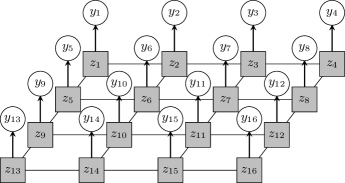
Figure 1: Graphical model for nearest fixed point distance, shown for a $4\times 4$ grid of pixels in the free depth map. At pixel $i$, the $Z_{i}\in\{\pm 1\}$ value is the unobserved inlier/outlier state, and $Y_{i}\in\operatorname{\mathbb{R}}_{\geq 0}$ is the observed distance to the closest fixed point.

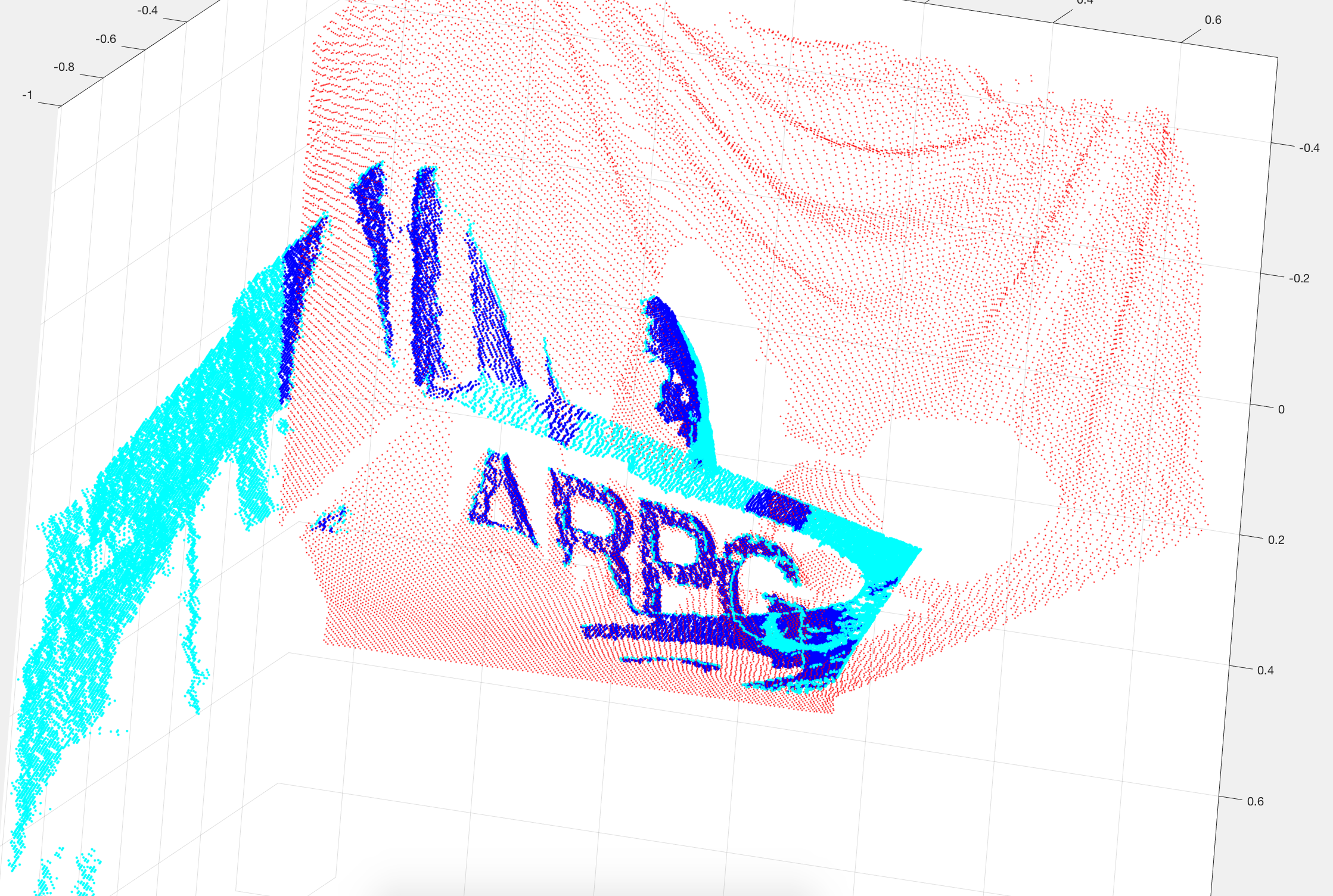
Figure 2: A successful registration with only 36% overlap. The red points are the fixed cloud (which have been downsampled in this view), to which the blue points have been aligned. The dark blue points are inliers and the light blue are outliers.

ICP attempts to determine the optimal transformation to align two point clouds. The algorithm recovers the transformation that moves the “free” point cloud onto the “fixed” point cloud. ICP proceeds by iteratively:

1. finding the closest point in the fixed cloud to each point in the free cloud;

2. discarding some of these matches as outliers; and

3. computing and applying the Euclidean transform that optimally aligns the remaining points, minimizing some measure of the distances to the nearest point found in step 1

until convergence. The present work focuses on step 2 of the above sequence.

Variations on step 3, depending on specifically what error metric is minimized [4], are explored further in Section 2. There are closed-form solutions [5] that minimize the point-to-point distance, including using the singular value decomposition [6] and the dual number quaternion method [7]. The present work minimizes the sum of squared point-to-point distances, for simplicity, although it is fundamentally independent of choice of error metric.

A crucial step in ICP is the rejection of outliers, generally resulting from non-overlapping volumes of space between two measurements. The original ICP formulation [1] did not discard any points and simply incurred error for each outlier. A proliferation of strategies have been proposed for discarding outliers [8, 9, 3, 10, 11, 12]. In the present work we propose an alternative method where the distribution of distances is modeled as a mixture of two Gaussians, one for inliers and one for outliers. Using a technique from image segmentation, a point’s inlier or outlier state is influenced by the state of its neighbors through a hidden Markov random field. The EM algorithm, with the use of a mean field approximation, allows for inference of the hidden state.

2 Related Work

Several attempts have been made to improve registration performance in the low-overlap regime. The hybrid genetic/hill-climbing algorithm of [13, 14] shows success with overlaps down to 55%. Good low-overlap performance is claimed in [15], which defines a “direction angle” on points and then aligns clouds in rotation using a histogram of these, and in translation using correlations of 2-D projections. Rotational alignment is recovered using extended Gaussian images in [2], and refined with ICP, showing success with overlap as low as 45%.

Use of robust statistics or error metrics besides sum of squared point-to-point distance has made ICP more robust to outliers. The point-to-plane [16] metric, where the distance is measured as it is projected onto the surfance normal of the fixed point, is frequently used and has been shown to be more robust in the case of limited overlap [17]. Color information can also be exploited [18, 19]. Sparse norms are used within ICP in [20], which can be sped up using simulated annealing [21].

Improvements to ICP have been achieved through better rejection of outlier correspondences. [8] applies a user-defined distance threshold, where matches beyond this threshold are discarded. Trimmed ICP uses fixed fraction of point correspondences (typically 90%) with smallest residuals [3]. Another approach uses a distance threshold of the mean distance plus 2.5 times the standard deviation of the distances [9]. The X84 criterion is similar, but uses the more robust median absolute deviation (MAD) in place of the standard deviation, and so rejects residuals more than 5.2 MADs above the median [10]. [11] presents an adaptive threshold which is tuned with a distance parameter which does not have direct physical significance. Yet another method [12] leverages the fact that distances between corresponding points within a cloud will be invariant under rigid motion and finds the largest set of consistent correspondences to identify inliers. Fractional ICP dynamically adapts the fraction of point correspondences to be used [22], although this method explicitly assumes a large fraction of overlap, with a penalty for smaller overlap fractions. In [23], points are classified as inliers or one of three classes of outliers: occluded, unpaired (outside the frame), or outliers (sensor noise). EM-ICP [24, 25] treats correspondence as a hidden variable and then computes assignment probabilities in the E-step, and the implied rigid transformation in the M-step, however, it is still assumed that every point in the free cloud corresponds to some point in the fixed cloud.

Since ICP requires good initialization, a significant body of work has been devoted to achieving global registration or finding an approximate alignment from any initial state, which is then refined with ICP. In [26, 27], an initial alignment is found by matching sets of 4 coplanar points, using ratios invariant to match sets; good performance with low overlap is claimed. Fast global registration between two or more point clouds is achieved in [28] by finding correspondences once based on point features, and then using robust estimators to ignore spurious correspondences. Kernel correlation [29] registers point clouds by minimizing the entropy of the resulting joint cloud. [30] minimizes the Hausdorff distance of several descriptors using particle swarm optimization to find the globally optimal alignment. LM-ICP [31] uses Levenberg-Marquardt to directly minimize the registration error over transformations and closest-point distances; derivatives for closest-point distances are precomputed with finite differences of a discretized distance transform.

Branch-and-bound algorithms can guarantee global optimality, and several variations have been applied to the registration problem [32, 33]. A branch-and-bound search for an initial alignment can be executed over rotations assuming the translation is known [34, 35], or over both rotations and translations [36]. Similarly, branch-and-bound has been employed for point or feature correspondences, such as [37], based on curvature features. Calculating bounds can be computationally intensive, and so finding bounds that are easily calculated offers appreciable speed-ups. For instance, [38] uses distributions of surface normals for rotation and Gaussian mixtures for translation.

Good feature descriptors for points in point clouds can help achieve global registration efficiently by finding corresponding points independent of their initial positions. Several feature descriptors are reviewed in [39]. Deep neural network auto-encoders also have been used to provide descriptors [40].

Finally, a variety of algorithms seek to register point clouds or shapes by representing them as probability densities. Several methods for generating and aligning these densities have been presented. NDT [41, 42, 43] uses a grid of normal distributions to describe the probability of observing a point at each possible location. Gaussian mixture models are frequently used to represent point clouds [44, 45]. Similarly, in [46] a depth image is registered to a truncated signed distance function representation of the target geometry. Non-rigid transforms are estimated in [47], using a GMM model for one cloud and selecting the transformation that maximizes the likelihood of observing the other cloud in that model.

Few of the above methods specifically address the problem of aligning clouds with little overlap—more often, it is assumed that only a small portion of the cloud will comprise unmatched points. By using an appropriate probabilistic model, this assumption need not be made, and the resulting method works equally well with high and low overlap.

3 Methodology

Let $i$ be a pixel position in the depth map generating the free cloud, and $B_{i}\in\operatorname{\mathbb{R}}^{4}$ be a point in the free cloud in homogenous coordinates. Let the fixed points be $C_{j}\in\operatorname{\mathbb{R}}^{4}$, again in homogenous coordinates. Note that the number of fixed points need not equal the number of free points.

In the first step of the ICP iteration we find,

$$I_{i}=\operatorname*{arg\,min}_{j}\lVert B_{i}-C_{j}\rVert.$$

We also save the associated distance,

$$Y_{i}=\min_{j}\lVert B_{i}-C_{j}\rVert=\lVert B_{i}-C_{I_{i}}\rVert.$$

The collected $Y_{i}$ random variables will be denoted $\bm{Y}$, with specific realizations denoted $y_{i}$ and $\bm{y}$, respectively.

The second step in the iteration makes use of these distance values to determine which point correspondences to consider inliers for the localization step,

$$S=\{i|\phi(i,Y_{i})\},$$

with some decision algorithm $\phi$.

Finally, the third step calculates the transformation,

$$T^{*}=\operatorname*{arg\,min}_{T}\sum_{i\in S}f(TB_{i},C_{I_{i}})$$

with $T\in\mathbb{SE}(3)$ and $f$ an error metric. For the point-to-point least-squares metric, which is used in this work, $f(TB_{i},C_{I_{i}})={\lVert TB_{i}-C_{I_{i}}\rVert}_{2}^{2}$.

For many sources of depth data, such as depth cameras or stereo matching, the points have an underlying 2-D lattice structure—the pixel grid. The pixel grid can be used to define neighbor relationships, so that a pixel not on the border of an image has four neighbors: up, down, left, and right. This method exploits these neighbor relations to model the distribution of the closest point distances $\bm{Y}$.

Given observed distances $\bm{y}$, we wish to decide which points are inliers. Our prior beliefs are:

• inliers will, on average, lie closer to their respective closest point than outliers; and

• pixel neighbors of inliers are likely inliers, and pixel neighbors of outliers are likely outliers.

To capture these priors, we model the distribution of $\bm{Y}$ as a mixture of two Gaussians, one for inliers and one for outliers, where a point’s mixture membership is dependent on its four nearest pixel neighbors. That is, we capture the second prior using a hidden Markov random field on the inlier/outlier state of a point. The graphical model is shown in Fig. 1. The distribution of $\bm{Y}$ is conditionally dependent on the hidden distribution $\bm{Z}$ which is Gibbs distributed. The maximum likelihood model parameters and hidden state can be estimated using the EM algorithm, with a mean field approximation for $\bm{Z}$, which does not require any Monte Carlo methods. This method is very similar to the image segmentation model presented in [48, 49, 50], which we follow closely, specializing its derivation to this application.

3.1 Hidden Markov random field model

Let $Z_{i}\in\{\pm 1\}$ represent the inlier/outlier state of the point generated from pixel $i$, with $-1$ indicating an outlier, and $+1$ indicating an inlier. Let $\bm{Z}$ represent the collection of all $Z_{i}$ states, and $\bm{z}$ represent a realization of $\bm{Z}$. Let $i\sim i^{\prime}$ indicate that two pixels $i$ and $i^{\prime}$ are neighbors. $\bm{Z}$ is a Markov random field, and is Gibbs distributed.

A Bayesian network can be factored into conditional distributions, which can be calculated directly. However, a Markov random field has undirected edges and so the distribution is calculated based on an energy function, $H(\bm{Z})$, from which the relative probability of different configurations can be calculated.

The Gibbs distribution is calculated based on the energy of a given configuration $\bm{z}$, appropriately normalized,

$$P_{G}(\bm{Z})=W^{-1}\exp(-H(\bm{Z})),$$

where $W$ is a normalization term called the “partition function”,

$$W=\sum_{\mathbf{z}}\exp(-H(\bm{z})).$$

We use the energy function, $H(\bm{z})=-\beta\sum_{i\sim i^{\prime}}z_{i}z_{i^{\prime}}$, where $\beta\geq 0$ is a parameter controlling the interaction strength ($\beta<0$ represents systems where we expect neighbors to be dissimilar, and when $\beta=0$ there is no interaction). Note that calculation of $W$, and therefore exact calculation of $P_{G}(\bm{z})$, requires a sum over all possible configurations $\bm{z}$, so is exponential in the number of pixels. For any nontrivial point cloud this is intractable. We avoid this issue with the mean field approximation, described below.

We assume $Y_{i}|Z_{i}\sim N(y_{i};\mu_{z_{i}},\sigma_{z_{i}})$, so the complete distribution, then, is

$$f(\bm{Y},\bm{Z}|\beta,\theta)=P_{G}(\bm{Z}|\beta)\prod_{i}N(y_{i}|\mu_{z_{i}},\sigma_{z_{i}})$$

with parameters $\{\beta,\mu_{-1},\sigma_{-1},\mu_{+1},\sigma_{+1}\}$. We will use $\theta$ to represent all Gaussian component parameters, that is, $\theta=\{\mu_{-1},\sigma_{-1},\mu_{+1},\sigma_{+1}\}$.

The mean field approximation assumes a fixed configuration $\bm{\tilde{z}}=\operatorname{\mathbb{E}}[P_{G}(\bm{Z}|\beta)]$, and approximates the Gibbs distribution with independent components conditioned on this fixed configuration,

$$P_{G}(\bm{Z}|\beta)\approx\prod_{i}P(Z_{i}|\beta,\bm{\tilde{z}}).$$

As the components are independent, it is no longer necessary to exhaust over all possible $\bm{z}$ configurations. Note that while $z_{i}\in\{-1,+1\}$, the mean field can take intermediate values, $\tilde{z}_{i}\in[-1,+1]$. The components also depend only on local information,

$$P(z_{i}|\beta,\bm{\tilde{z}})=\frac{\exp\left(\beta\sum_{i\sim i^{\prime}}z_{i}\tilde{z}_{i^{\prime}}\right)}{\exp\left(\beta\sum_{i\sim i^{\prime}}(+1)\tilde{z}_{i^{\prime}}\right)+\exp\left(\beta\sum_{i\sim i^{\prime}}(-1)\tilde{z}_{i^{\prime}}\right)}.$$

The final complete likelihood with the mean field approximation is then,

$$f(\bm{Y},\bm{Z}|\beta,\theta)=P(z_{i}|\beta,\bm{\tilde{z}})N(y_{i}|\mu_{z_{i}},\sigma_{z_{i}}),$$

and the log likelihood is,

$$\log f(\bm{Y},\bm{Z}|\beta,\theta)=\\ \sum_{i}\left(\beta\sum_{i\sim i^{\prime}}z_{i}\tilde{z}_{i^{\prime}}-\right.\log\left(\exp\left(\beta\sum_{i\sim i^{\prime}}(+1)\tilde{z}_{i^{\prime}}\right)+\exp\left(\beta\sum_{i\sim i^{\prime}}(-1)\tilde{z}_{i^{\prime}}\right)\right)\\ \left.-\frac{1}{2}\sigma_{z_{i}}-\frac{{(y_{i}-\mu_{z_{i}})}^{2}}{2\sigma_{z_{i}}^{2}}\right)+\text{const}.$$

3.2 Applying the EM algorithm

With this approximation, the EM algorithm [51] can be adapted to find the maximum likelihood estimate of the parameters $\theta$ and the hidden field. The $\beta$ value could be estimated as well, but we simply use the value 2, which gives satisfying results. Initially, we assume that the 10% of points with the greatest distance to their corresponding closest point are outliers and so set $\bm{\tilde{z}}^{(0)}$ accordingly. Similarly, $\theta^{(0)}$ is initialized with the means and standard deviations of the two sets. The EM iteration then proceeds as follows,

• E-step:

  $$\bm{\tilde{z}}^{(q+1)}\coloneqq\operatorname{\mathbb{E}}_{\text{mf}}[\bm{Z}|\bm{y},\bm{\tilde{z}}^{(q)},\theta^{(q)}];$$

• M-step:

  $$\theta^{(q+1)}\coloneqq\operatorname*{arg\,max}_{\theta}f(\bm{Y},\bm{Z}|\beta,\theta)|\bm{y},\bm{\tilde{z}}^{(q+1)}.$$

We integrate this into the ICP algorithm by using the resulting $\bm{\tilde{z}}^{(q+1)}$ values to select inliers. We consider EM to have converged when all corresponding values in $\bm{\tilde{z}}^{(q+1)}$ and $\bm{\tilde{z}}^{(q)}$ have the same sign. Due to the potential for oscillatory behavior, we also compare $\bm{\tilde{z}}^{(q+1)}$ and $\bm{\tilde{z}}^{(q-1)}$.

Ideally, we would run EM to convergence within each ICP step. However, we limit the number of EM iterations to ensure adequate performance. Since the initial assumptions may be poor, we allow more EM iterations before calculating and applying the first transformation. Within each ICP step, EM is limited to 20 iterations, but initially it is allowed to run up to 600 steps, which allowed for convergence in most cases. The full procedure is shown in Algorithm 1.

3.2.1 The E-step

With the mean field approximation, this step is similar to the E-step of a simple Gaussian mixture model, although each point has its own prior distribution on component membership. The update is independent for each point, and is calculated

$$\tilde{z}_{i}^{(q+1)}=\frac{\sum_{z_{i}}z_{i}\exp\left(\beta\sum_{i\sim i^{\prime}}z_{i}\tilde{z}_{i^{\prime}}^{(q)}-\log\sigma_{z_{i}}-0.5\sigma_{z_{i}}^{-2}{(y_{i}-\mu_{z_{i}})}^{2}\right)}{\sum_{z_{i}}\exp\left(\beta\sum_{i\sim i^{\prime}}z_{i}\tilde{z}_{i^{\prime}}^{(q)}-\log\sigma_{z_{i}}-0.5\sigma_{z_{i}}^{-2}{(y_{i}-\mu_{z_{i}})}^{2}\right)}.$$

Note that [50] recommends a sequential update, but this is simultaneous, which is both embarrassingly parallel and easier to implement.

3.2.2 The M-step

The $\tilde{z}_{i}^{(q+1)}$ values calculated in the E-step are simply linear transformations of the current estimate of $P(Z_{i}=z_{i})$,

$$P^{(q+1)}(Z_{i}=z_{i})=\frac{1+z_{i}\tilde{z}_{i}^{(q+1)}}{2},$$

so the M-step update is simply,

$$\mu_{z_{i}}^{(q+1)} =\frac{\sum_{i}P^{(q+1)}(Z_{i}=z_{i})Y_{i}}{\sum_{i}P^{(q+1)}(Z_{i}=z_{i})}$$

$$\sigma_{z_{i}}^{(q+1)} =\frac{\sum_{i}P^{(q+1)}(Z_{i}=z_{i}){(Y_{i}-\mu_{z_{i}}^{(q+1)})}^{2}}{\sum_{i}P^{(q+1)}(Z_{i}=z_{i})}.$$

Input: $T_{\text{init}}$, $\bm{B}$, $\bm{C}$, $\beta$, thresholds

KDtree = BuildKdTree$(\bm{C})$

$T=T_{\text{init}}$

$\bm{B}=T\times\bm{B}$

$\bm{I},\bm{Y}$ = KDtree.NearestNeighbors$(\bm{B})$

Initialize $\bm{z}$ to 1 except for highest 10% of $\bm{Y}$, which are initialized to -1.

do

       $\theta$ = M-step$(\bm{Y},\bm{z})$

      $\bm{z}$ = E-step$(\bm{Y},\theta,\beta)$

while some $\bm{z}$ value changed sign and iters $<$ 600;

do

      

      do

             $\theta$ = M-step$(\bm{Y},\bm{z})$

            $\bm{z}$ = E-step$(\bm{Y},\theta,\beta)$

      while some $\bm{z}$ value changed sign and iters $<$ 20;

      $T_{\text{step}}$ = localize$(\bm{B},\bm{C},\bm{z})$

      $T=T_{\text{step}}\times T$

      $\bm{B}=T_{\text{step}}\times\bm{B}$

      $\bm{I},\bm{Y}$ = KDtree.NearestNeighbors$(\bm{B})$

while convergence thresholds not met and iters $<$ 50;

return T

Algorithm 1 The full HMRF ICP algorithm

4 Experiments

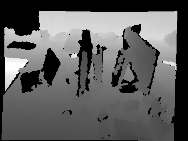
Figure 3: Fixed frames, RGB (not used in alignment) and depth maps.

The method is compared with five other outlier rejection methods: no outlier rejection, keeping 90% of the points with smallest residuals, keeping points whose residuals were less than 2.5 standard deviations above the mean, keeping points whose residuals were less than 5.2 median absolute deviations above the median (the so-called “X84” criterion), and the dynamic threshold from [11]. These are referred to as “all”, “percent”, “sigma”, “X84”, and “dynamic”, respectively.

The method is applied to two datasets: the shark sequence is a tabletop scene, taken by an Asus Xtion Pro; the desk sequence is a publicly available RGB-D SLAM dataset [52]. Ground truth poses are known for both sequences. The sensor in the desk sequence is tracked using an external motion tracking system, operating at 100Hz, from which poses at shutter timestamps are interpolated. The poses in the shark sequence are those estimated in the tracking stage of InfiniTAM[53] during the reconstruction of the scene. The intrinsic camera calibration for the desk sequence is provided with the data and the Xtion Pro was calibrated so that the depth maps could be unprojected appropriately and converted to point clouds.

In each case, one frame is chosen as the reference frame, shown in Fig. 3, and then a number of other frames with varying fractions of overlap are aligned to it. The remaining frames are a random sample stratified to include a variety of overlap ratios the with fixed frame. The overlap with the fixed frame is estimated using the ground truth poses and the distance to each point’s nearest neighbor in its own cloud versus in the fixed cloud.

In the full shark sequence, the smallest overlap is about 35%, and the largest nearly 100%. The sample of 40 frames is selected with 5 frames from each decile (30% to 40%, 40% to 50%, etc.), and 5 frames selected at random from all the frames.

The desk sequence includes frames that do not overlap at all with the reference frame; these frames are discarded. However, the sample includes frames with less than 1% overlap. The sample is again a stratified random sample, with 5 frames selected from each decile, for a total of 50 frame.

5 Results

For each free frame, 16 initializations were tested. These were generated by aligning each frame to the fixed frame using the ground truth poses, and then perturbing this alignment by a rotation of $\pi/30$ around each of 16 random axes, centered at the cloud centroid. The same 16 axes were used for all frames. All experiments were executed in MATLAB on a workstation with 8 Intel^® Xeon^® E5620 CPUs at 2.40GHz, and with 48 Gb RAM. All code can be found at https://github.com/JStech/ICP.

Figs. 4 and 5 show the results, plotted against overlap fraction. The translation error is the norm of the error vector (measured in meters). The rotation error is the angle in radians. Finally, the number of ICP iterations until convergence, as well as total elapsed time are also shown. A small amount of jitter has been added to the x-axis in all plots, to allow for better visual inspection of the data. The plot of iterations also has y-axis jitter.

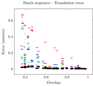
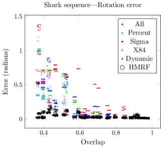
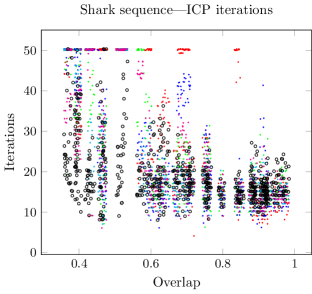
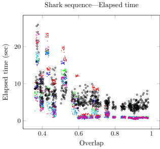
Figure 4: Shark sequence results

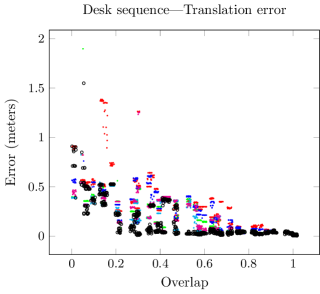
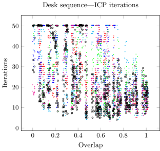
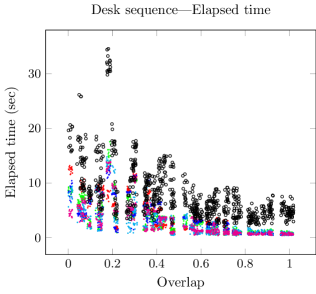
Figure 5: Desk sequence results

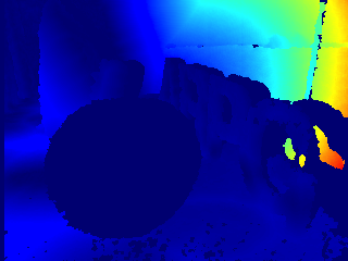
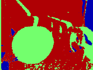
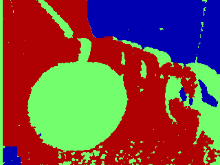
Figure 6: Example $\bm{Y}$, $\bm{\tilde{z}}^{(1)}$, and $\bm{\tilde{z}}^{(370)}$ (at convergence). This frame has 36% overlap with the fixed frame. The left image shows the observed distance to the nearest fixed point in the initial configuration; red is farther, blue is nearer, and the darkest blue areas are unobserved. In the right two images, blue pixels are outliers and red pixels are inliers, green pixels are unobserved.

At moderate to low overlaps, the HMRF method recovers a more accurate transformation and does so in fewer iterations. To see why, consider the example frame with 36% overlap shown in Fig. 6. The three images all represent values before the first transformation is applied to the free cloud: the first is the residual distance to the nearest fixed point, the second is the initial setting of the $\bm{\tilde{z}}$ field, and the third is the converged $\bm{\tilde{z}}$ field before the first iteration of ICP. The HMRF model flexibly adapts to the small proportion of inlier points, in particular it eliminates outliers across the top of the image. The unobserved pixels occupy 31% of the image. In the initial $\bm{\tilde{z}}$ field, 62% of pixels are considered inliers, and the remaining 7% are considered outliers. After 370 initial EM iterations, the $\bm{\tilde{z}}$ field has converged, and now has only 49% inliers and 20% outliers. By eliminating these outliers before the first transformation is calculated, divergence from the nearby optimum is avoided. The point clouds after final registration for this frame can be seen in Fig. 2.

HMRF ICP performs well for all frames in the shark sequence, with a maximum of 0.017 m translation error and 0.0776 radians rotation error for clouds with 60% or more overlap; the maximum error for all shark frames is 0.036 m and 0.196 radians. Furthermore, although HMRF ICP is slower than the other methods at high overlap, it shows very little slowing as overlap decreases, so these low errors were achieved faster than the poor results of the other methods.

The performance is not as good with the desk sequence. Three regimes are evident in the results: above 50% overlap, between 20% and 50%, and below 20%. The maximum error on frames with 50% or more overlap is 0.077 m and 0.109 radians, and 0.386 m and 0.317 radians with 20% or more overlap. Below 20% overlap, performance degrades severely, with maximum errors of 1.55 m and 1.97 radians.

An example alignment is shown at https://youtu.be/w4eVOgd7Zes.

6 Conclusion

The HMRF model for inliers and outliers in a depth map being aligned via ICP has demonstrated advantages in the low overlap regime without sacrificing performance at high overlap. The HMRF model describes observed inlier/outlier behavior well, and so can adapt to the situation. This proves particularly useful in the construction of models from 3-D scanner data, as fewer scans would be required. There are numerous improvements that could be pursued for future research. The Gaussian distribution was chosen for convenience, but it is unlikely that residuals of either inliers or outliers are distributed normally. It would be straightforward to use different distributions, which could be selected by investigating the empirical inlier and outlier residual distributions. This method also assumes an underlying grid topology for the free cloud, which precludes it from use with a variety of sensors, such as rotating LiDAR sensors. It could be extended to general, unstructured point clouds by defining appropriate neighbor relations and energy function, $H(\bm{z})$. Finally, many of the improvements to ICP detailed in Section 2 could be incorporated to expand the basin of convergence or otherwise improve performance.

7 Acknowledgements

The authors thank Nisar Ahmed for his helpful insight. JS was supported by the U.S. Department of Defense (DoD) through the National Defense Science & Engineering Graduate Fellowship (NDSEG) program while conducting this work. CH was supported by DARPA award no. N65236–16–1–1000.

References

- [1] P. J. Besl, N. D. McKay, et al., “A method for registration of 3-d shapes,” IEEE Transactions on Pattern Analysis and Machine Intelligence, vol. 14, no. 2, pp. 239–256, 1992.
- [2] A. Makadia, A. Patterson, and K. Daniilidis, “Fully automatic registration of 3d point clouds,” in Computer Vision and Pattern Recognition, 2006 IEEE Computer Society Conference on, vol. 1, pp. 1297–1304, IEEE, 2006.
- [3] D. Chetverikov, D. Svirko, D. Stepanov, and P. Krsek, “The trimmed iterative closest point algorithm,” in Pattern Recognition, 2002. Proceedings. 16th International Conference on, vol. 3, pp. 545–548, IEEE, 2002.
- [4] S. Rusinkiewicz and M. Levoy, “Efficient variants of the ICP algorithm,” in 3-D Digital Imaging and Modeling, 2001. Proceedings. Third International Conference on, pp. 145–152, IEEE, 2001.
- [5] D. W. Eggert, A. Lorusso, and R. B. Fisher, “Estimating 3-d rigid body transformations: a comparison of four major algorithms,” Machine vision and applications, vol. 9, no. 5-6, pp. 272–290, 1997.
- [6] K. S. Arun, T. S. Huang, and S. D. Blostein, “Least-squares fitting of two 3-d point sets,” IEEE Transactions on Pattern Analysis and Machine Intelligence, no. 5, pp. 698–700, 1987.
- [7] M. W. Walker, L. Shao, and R. A. Volz, “Estimating 3-d location parameters using dual number quaternions,” CVGIP: Image Understanding, vol. 54, no. 3, pp. 358–367, 1991.
- [8] G. Turk and M. Levoy, “Zippered polygon meshes from range images,” in Proceedings of the 21st Annual Conference on Computer Graphics and Interactive Techniques, pp. 311–318, ACM, 1994.
- [9] T. Masuda, K. Sakaue, and N. Yokoya, “Registration and integration of multiple range images for 3-d model construction,” in Pattern Recognition, 1996., Proceedings of the 13th International Conference on, vol. 1, pp. 879–883, IEEE, 1996.
- [10] A. Fusiello, U. Castellani, L. Ronchetti, and V. Murino, “Model acquisition by registration of multiple acoustic range views,” Computer Vision—ECCV 2002, pp. 558–559, 2002.
- [11] Z. Zhang, “Iterative point matching for registration of free-form curves and surfaces,” International Journal of Computer Vision, vol. 13, no. 2, pp. 119–152, 1994.
- [12] O. Enqvist, K. Josephson, and F. Kahl, “Optimal correspondences from pairwise constraints,” in Computer Vision, 2009 IEEE 12th International Conference on, pp. 1295–1302, IEEE, 2009.
- [13] L. Silva, O. R. Bellon, K. L. Boyer, and P. F. Gotardo, “Low-overlap range image registration for archaeological applications,” in Computer Vision and Pattern Recognition Workshop, 2003. CVPRW’03. Conference on, vol. 1, pp. 9–9, IEEE, 2003.
- [14] L. Silva, O. R. P. Bellon, and K. L. Boyer, “Precision range image registration using a robust surface interpenetration measure and enhanced genetic algorithms,” IEEE transactions on pattern analysis and machine intelligence, vol. 27, no. 5, pp. 762–776, 2005.
- [15] Y. Ma, Y. Guo, J. Zhao, M. Lu, J. Zhang, and J. Wan, “Fast and accurate registration of structured point clouds with small overlaps,” in The IEEE Conference on Computer Vision and Pattern Recognition (CVPR) Workshops, June 2016.
- [16] Y. Chen and G. Medioni, “Object modeling by registration of multiple range images,” in Robotics and Automation, 1991. Proceedings., 1991 IEEE International Conference on, pp. 2724–2729, IEEE, 1991.
- [17] J. Salvi, C. Matabosch, D. Fofi, and J. Forest, “A review of recent range image registration methods with accuracy evaluation,” Image and Vision computing, vol. 25, no. 5, pp. 578–596, 2007.
- [18] A. E. Johnson and S. B. Kang, “Registration and integration of textured 3d data,” Image and Vision Computing, vol. 17, no. 2, pp. 135–147, 1999.
- [19] H. Men, B. Gebre, and K. Pochiraju, “Color point cloud registration with 4D ICP algorithm,” in Robotics and Automation (ICRA), 2011 IEEE International Conference on, pp. 1511–1516, IEEE, 2011.
- [20] S. Bouaziz, A. Tagliasacchi, and M. Pauly, “Sparse iterative closest point,” in Computer graphics forum, vol. 32, pp. 113–123, Wiley Online Library, 2013.
- [21] P. Mavridis, A. Andreadis, and G. Papaioannou, “Efficient sparse icp,” Computer Aided Geometric Design, vol. 35, pp. 16–26, 2015.
- [22] J. M. Phillips, R. Liu, and C. Tomasi, “Outlier robust icp for minimizing fractional rmsd,” in 3-D Digital Imaging and Modeling, 2007. 3DIM’07. Sixth International Conference on, pp. 427–434, IEEE, 2007.
- [23] T. Masuda and N. Yokoya, “A robust method for registration and segmentation of multiple range images,” Computer vision and image understanding, vol. 61, no. 3, pp. 295–307, 1995.
- [24] S. Granger and X. Pennec, “Multi-scale em-icp: A fast and robust approach for surface registration,” in European Conference on Computer Vision, pp. 418–432, Springer, 2002.
- [25] J. Hermans, D. Smeets, D. Vandermeulen, and P. Suetens, “Robust point set registration using em-icp with information-theoretically optimal outlier handling,” in Computer Vision and Pattern Recognition (CVPR), 2011 IEEE Conference on, pp. 2465–2472, IEEE, 2011.
- [26] D. Aiger, N. J. Mitra, and D. Cohen-Or, “4-points congruent sets for robust pairwise surface registration,” ACM Transactions on Graphics (TOG), vol. 27, no. 3, p. 85, 2008.
- [27] N. Mellado, D. Aiger, and N. J. Mitra, “Super 4pcs fast global pointcloud registration via smart indexing,” in Computer Graphics Forum, vol. 33, pp. 205–215, Wiley Online Library, 2014.
- [28] Q.-Y. Zhou, J. Park, and V. Koltun, “Fast global registration,” in European Conference on Computer Vision, pp. 766–782, Springer, 2016.
- [29] Y. Tsin and T. Kanade, “A correlation-based approach to robust point set registration,” in European conference on computer vision, pp. 558–569, Springer, 2004.
- [30] M. Yousrya, B. A. Youssef, M. A. El Azizc, and F. I. Sidkyc, “3d point cloud registration using particle swarm optimization based on different descriptors,”
- [31] A. W. Fitzgibbon, “Robust registration of 2D and 3D point sets,” Image and Vision Computing, vol. 21, no. 13, pp. 1145–1153, 2003.
- [32] C. Olsson, F. Kahl, and M. Oskarsson, “Branch-and-bound methods for euclidean registration problems,” IEEE Transactions on Pattern Analysis and Machine Intelligence, vol. 31, no. 5, pp. 783–794, 2009.
- [33] C. Papazov and D. Burschka, “Stochastic global optimization for robust point set registration,” Computer Vision and Image Understanding, vol. 115, no. 12, pp. 1598–1609, 2011.
- [34] A. Parra Bustos, T.-J. Chin, and D. Suter, “Fast rotation search with stereographic projections for 3d registration,” in Proceedings of the IEEE Conference on Computer Vision and Pattern Recognition, pp. 3930–3937, 2014.
- [35] H. Li and R. Hartley, “The 3d-3d registration problem revisited,” in Computer Vision, 2007. ICCV 2007. IEEE 11th International Conference on, pp. 1–8, IEEE, 2007.
- [36] J. Yang, H. Li, D. Campbell, and Y. Jia, “Go-icp: a globally optimal solution to 3d icp point-set registration,” IEEE transactions on pattern analysis and machine intelligence, vol. 38, no. 11, pp. 2241–2254, 2016.
- [37] N. Gelfand, N. J. Mitra, L. J. Guibas, and H. Pottmann, “Robust global registration,” in Symposium on geometry processing, vol. 2, p. 5, 2005.
- [38] J. Straub, T. Campbell, J. P. How, and J. W. Fisher III, “Efficient global point cloud alignment using bayesian nonparametric mixtures,”
- [39] Y. Guo, M. Bennamoun, F. Sohel, M. Lu, J. Wan, and N. M. Kwok, “A comprehensive performance evaluation of 3d local feature descriptors,” International Journal of Computer Vision, vol. 116, no. 1, pp. 66–89, 2016.
- [40] G. Elbaz, T. Avraham, and A. Fischer, “3d point cloud registration for localization using a deep neural network auto-encoder,” in The IEEE Conference on Computer Vision and Pattern Recognition (CVPR), July 2017.
- [41] P. Biber and W. Straßer, “The normal distributions transform: A new approach to laser scan matching,” in Intelligent Robots and Systems, 2003.(IROS 2003). Proceedings. 2003 IEEE/RSJ International Conference on, vol. 3, pp. 2743–2748, IEEE, 2003.
- [42] M. Magnusson, A. Lilienthal, and T. Duckett, “Scan registration for autonomous mining vehicles using 3d-ndt,” Journal of Field Robotics, vol. 24, no. 10, pp. 803–827, 2007.
- [43] M. Magnusson, A. Nuchter, C. Lorken, A. J. Lilienthal, and J. Hertzberg, “Evaluation of 3d registration reliability and speed-a comparison of icp and ndt,” in Robotics and Automation, 2009. ICRA’09. IEEE International Conference on, pp. 3907–3912, IEEE, 2009.
- [44] B. Jian and B. C. Vemuri, “A robust algorithm for point set registration using mixture of gaussians,” in Computer Vision, 2005. ICCV 2005. Tenth IEEE International Conference on, vol. 2, pp. 1246–1251, IEEE, 2005.
- [45] D. Campbell and L. Petersson, “An adaptive data representation for robust point-set registration and merging,” in Proceedings of the IEEE International Conference on Computer Vision, pp. 4292–4300, 2015.
- [46] E. Bylow, J. Sturm, C. Kerl, F. Kahl, and D. Cremers, “Real-time camera tracking and 3d reconstruction using signed distance functions.,” in Robotics: Science and Systems, vol. 2, 2013.
- [47] A. Myronenko and X. Song, “Point set registration: Coherent point drift,” IEEE transactions on pattern analysis and machine intelligence, vol. 32, no. 12, pp. 2262–2275, 2010.
- [48] Z. Kato and T.-C. Pong, “A markov random field image segmentation model for color textured images,” Image and Vision Computing, vol. 24, no. 10, pp. 1103–1114, 2006.
- [49] J. Besag, “On the statistical analysis of dirty pictures,” Journal of the Royal Statistical Society. Series B (Methodological), pp. 259–302, 1986.
- [50] G. Celeux, F. Forbes, and N. Peyrard, “EM procedures using mean field-like approximations for Markov model-based image segmentation,” Pattern recognition, vol. 36, no. 1, pp. 131–144, 2003.
- [51] A. P. Dempster, N. M. Laird, and D. B. Rubin, “Maximum likelihood from incomplete data via the EM algorithm,” Journal of the Royal Statistical Society. Series B (Methodological), pp. 1–38, 1977.
- [52] J. Sturm, N. Engelhard, F. Endres, W. Burgard, and D. Cremers, “A benchmark for the evaluation of rgb-d slam systems,” in Proc. of the International Conference on Intelligent Robot Systems (IROS), Oct. 2012.
- [53] O. Kähler, V. A. Prisacariu, C. Y. Ren, X. Sun, P. Torr, and D. Murray, “Very high frame rate volumetric integration of depth images on mobile devices,” IEEE transactions on visualization and computer graphics, vol. 21, no. 11, pp. 1241–1250, 2015.