Efficient D-optimal design of experiments for infinite-dimensional Bayesian linear inverse problems

Abstract

We develop a computational framework for D-optimal experimental design for PDE-based Bayesian linear inverse problems with infinite-dimensional parameters. We follow a formulation of the experimental design problem that remains valid in the infinite-dimensional limit. The optimal design is obtained by solving an optimization problem that involves repeated evaluation of the log-determinant of high-dimensional operators along with their derivatives. Forming and manipulating these operators is computationally prohibitive for large-scale problems. Our methods exploit the low-rank structure in the inverse problem in three different ways, yielding efficient algorithms. Our main approach is to use randomized estimators for computing the D-optimal criterion, its derivative, as well as the Kullback–Leibler divergence from posterior to prior. Two other alternatives are proposed based on low-rank approximation of the prior-preconditioned data misfit Hessian, and a fixed low-rank approximation of the prior-preconditioned forward operator. Detailed error analysis is provided for each of the methods, and their effectiveness is demonstrated on a model sensor placement problem for initial state reconstruction in a time-dependent advection-diffusion equation in two space dimensions.

35R30; 62K05; 68W20; 35Q62; 65C60; 62F15.

1 Introduction

Mathematical models of physical systems enable predictions of future outcomes. These mathematical models—typically described by a system of partial differential equations (PDEs)—often contain parameters such as initial conditions, boundary data, or coefficient functions that are unspecified and have to be estimated. This estimation requires solving inverse problems where one uses experimental data and the model to infer unknown model parameters. Experimental design is the process of specifying how measurement data, used in parameter inversion, are collected. On the one hand, the quantity and quality of data can critically impact the accuracy of parameter reconstruction. On the other hand, acquisition of experimental data is an expensive process that requires the deployment of scarce resources. Hence, it is of great practical importance to optimize the design of experiments so as to maximize the information gained in the parameter estimation or reconstruction.

Optimal experimental design (OED) controls experimental conditions by optimizing certain design criteria subject to physical or budgetary constraints. In large-scale applications, using commonly used experimental design criteria requires repeated evaluations of functionals (e.g., trace or determinant) of high dimensional and expensive-to-apply operators—applications of these operators to vectors involve expensive PDE solves. This is a fundamental challenge in OED for large-scale PDE-based Bayesian inverse problems for which we develop novel algorithms.

In our target applications, the Bayesian inverse problem seeks to infer an infinite-dimensional parameter using experimental measurements, which are collected at a set of sensor locations. The OED problem aims to find an optimal placement of sensors that optimize the statistical quality of the inferred parameter. We focus on D-optimal design of sensor networks at which observational data are collected. That is, we seek sensor placements that maximize the expected information gain in parameter inversion. Our approach, however, is general in that it is applicable to D-optimal experimental design for a broad class of linear inverse problems.

Related Work

OED is a thriving area of research [45, 6, 36, 34, 13, 9, 29, 21, 24, 16, 26, 32, 27, 3, 31, 46, 5, 2, 11, 17, 49, 47, 37]. In particular, A-optimal experimental design for large-scale applications has been addressed in [20, 21, 24, 22, 43, 3, 4, 17]. Computing A-optimal designs for large-scale applications faces similar challenges to the D-optimal designs. The use of Monte-Carlo trace estimators [7] has been instrumental in making A-optimal design computationally feasible for such applications.

Fast algorithms for computing expected information gain, i.e., the D-optimal criterion, for nonlinear inverse problems, via Laplace approximations, were proposed in [31, 32]. The focus of the aforementioned works was efficient computation of the D-optimal criterion. The optimal design was then computed by an exhaustive search over prespecified sets of experimental scenarios. We also mention [26, 27, 28] that use polynomial chaos (PC) expansions to build easy-to-evaluate surrogates of the forward model. The expected information gain is then evaluated using an appropriate Monte Carlo procedure. In [27, 28], the authors use a gradient based approach to obtain the optimal design. In [44], the authors propose an alternate design criterion given by a lower bound of the expected information gain, and use PC representation of the forward model to accelerate objective function evaluations. However, the approaches based on PC representations remain limited in scope to problems with low to moderate parameter dimensions (e.g., parameter dimensions in order of tens).

Efficient estimators for the evaluation of D-optimal criterion were developed in [39, 38]; however, these works do not discuss the problem of computing D-optimal designs. The mathematical formulation of Bayesian D-optimality for infinite-dimensional Bayesian linear inverse problems was established in [2]. A scalable solver for D-optimal designs for infinite-dimensional Bayesian inverse problems, however, is currently not available to the best of our knowledge. Here by scalable we mean methods whose computational complexity, in terms of the number of required PDE solves, do not scale with the dimension of the discretized inversion parameter.

Contributions

We propose a general computational framework for D-optimal experimental design for infinite-dimensional Bayesian linear inverse problems governed by PDEs, with Gaussian prior and noise models. Specifically, we propose three approaches for approximately computing the D-optimal criterion, its gradient, and the Kullback–Leibler (KL) divergence from the posterior to prior: (i) truncated spectral decomposition approach; (ii) randomized approach; and (iii) an approach based on fixed low-rank approximation of the prior-preconditioned forward operator. We compare and contrast the different approaches and perform a detailed error analysis for each case. The effectiveness of the algorithms is illustrated on a model problem involving initial state inversion in a time-dependent advection-diffusion equation. Besides the computational framework, we show the relationship between the expected KL divergence and the D-optimal design criterion; while this is addressed in [2], in the infinite-dimensional Hilbert space setting, we present a simple derivation within the context of the discretized problem, which leads to the D-optimal criterion that is meaningful in the infinite-dimensional limit.

Paper overview

In section 2, we review the Bayesian formulation of the inverse problem in infinite dimensions, with special attention to discretization and finite dimensional representation. We also review our recent work [38] on randomized estimators for determinants. In section 3, we provide a simple derivation of the Bayesian D-optimal criterion for infinite-dimensional problems and present the formulation of the sensor placement problem as a D-optimal design problem. Section 4 is devoted to developing efficient algorithms for computing the KL divergence from posterior to prior, and for evaluating the D-optimal objective function and its gradient; also, in that section, we formulate the optimization problem for finding D-optimal sensor placements. In section 5, we outline our model sensor placement problem for initial state inversion in a time-dependent advection-diffusion equation. Section 6 contains our numerical results, where we illustrate effectiveness of our methods. Finally, in section 7, we provide some concluding remarks.

2 Background

In this section, we provide the requisite background material required for the formulation and numerical computation of optimal experimental designs for infinite-dimensional Bayesian inverse problems.

2.1 Bayesian linear inverse problems

Here, we describe the main ingredients of a Bayesian linear inverse problem, and our assumptions about them. The inference parameter is denoted by $\theta$ and is an element of an infinite-dimensional real separable Hilbert space $\mathcal{V}$. We consider a Gaussian measure $\mu_{\text{pr}}=\mathcal{N}\!\left({\theta_{\mathup{pr}}},{\mathcal{C}_{\mathup{pr}}}\right)$ as the prior distribution law of $\theta$. The prior mean $\theta_{\mathup{pr}}$ is assumed to be a sufficiently regular element of $\mathcal{V}$, and $\mathcal{C}_{\mathup{pr}}:\mathcal{V}\to\mathcal{V}$ a strictly positive self-adjoint trace-class operator. Following [12, 40, 18], we consider prior covariance operators of the form $\mathcal{C}=\mathcal{A}^{-2}$, where $\mathcal{A}$ is a Laplacian-like operator (in the sense defined in [40]). This ensures that, in two and three space dimensions, $\mathcal{C}$ is trace-class.

We consider observations taken at ${n_{s}}$ measurement points, which henceforth we refer to as sensor locations, and at ${n_{t}}$ discrete points in time. We denote the vector of experimental (sensor) data by ${\mathchoice{\mbox{\boldmath$\displaystyle{y}$}}{\mbox{\boldmath$\textstyle{y}$}}{\mbox{\boldmath$\scriptstyle{y}$}}{\mbox{\boldmath$\scriptscriptstyle{y}$}}}\in\mathbb{R}^{n_{y}}$, where ${n_{y}}={n_{s}}{n_{t}}$. We assume an additive Gaussian noise model,

$${\mathchoice{\mbox{\boldmath$\displaystyle{y}$}}{\mbox{\boldmath$\textstyle{y}$}}{\mbox{\boldmath$\scriptstyle{y}$}}{\mbox{\boldmath$\scriptscriptstyle{y}$}}}=F\theta+{\mathchoice{\mbox{\boldmath$\displaystyle{\eta}$}}{\mbox{\boldmath$\textstyle{\eta}$}}{\mbox{\boldmath$\scriptstyle{\eta}$}}{\mbox{\boldmath$\scriptscriptstyle{\eta}$}}},\quad{\mathchoice{\mbox{\boldmath$\displaystyle{\eta}$}}{\mbox{\boldmath$\textstyle{\eta}$}}{\mbox{\boldmath$\scriptstyle{\eta}$}}{\mbox{\boldmath$\scriptscriptstyle{\eta}$}}}\sim\mathcal{N}\!\left({{\mathchoice{\mbox{\boldmath$\displaystyle{0}$}}{\mbox{\boldmath$\textstyle{0}$}}{\mbox{\boldmath$\scriptstyle{0}$}}{\mbox{\boldmath$\scriptscriptstyle{0}$}}}},{{\mathchoice{\mbox{\boldmath$\displaystyle{\Gamma}$}}{\mbox{\boldmath$\textstyle{\Gamma}$}}{\mbox{\boldmath$\scriptstyle{\Gamma}$}}{\mbox{\boldmath$\scriptscriptstyle{\Gamma}$}}}_{\!\mathup{noise}}}\right).$$

Here ${\mathchoice{\mbox{\boldmath$\displaystyle{\Gamma}$}}{\mbox{\boldmath$\textstyle{\Gamma}$}}{\mbox{\boldmath$\scriptstyle{\Gamma}$}}{\mbox{\boldmath$\scriptscriptstyle{\Gamma}$}}}_{\!\mathup{noise}}\in\mathbb{R}^{{n_{y}}\times{n_{y}}}$ is the noise covariance matrix, and $F:\mathcal{V}\to\mathbb{R}^{n_{y}}$ is a linear parameter-to-observable map, whose evaluation involves solving the governing PDEs, and applying an observation operator that extracts solution values at the sensor locations and at observation times. Due to our choice of the noise model, the likelihood probability density function (pdf), $\pi_{\mathup{like}}({\mathchoice{\mbox{\boldmath$\displaystyle{y}$}}{\mbox{\boldmath$\textstyle{y}$}}{\mbox{\boldmath$\scriptstyle{y}$}}{\mbox{\boldmath$\scriptscriptstyle{y}$}}}|\theta)$, is given by

$$\pi_{\mathup{like}}({\mathchoice{\mbox{\boldmath$\displaystyle{y}$}}{\mbox{\boldmath$\textstyle{y}$}}{\mbox{\boldmath$\scriptstyle{y}$}}{\mbox{\boldmath$\scriptscriptstyle{y}$}}}\mid\theta)\propto\exp\left\{-\frac{1}{2}\big{(}F\theta-{\mathchoice{\mbox{\boldmath$\displaystyle{y}$}}{\mbox{\boldmath$\textstyle{y}$}}{\mbox{\boldmath$\scriptstyle{y}$}}{\mbox{\boldmath$\scriptscriptstyle{y}$}}}\big{)}^{\mkern-1.5mu\mathsf{T}}{\mathchoice{\mbox{\boldmath$\displaystyle{\Gamma}$}}{\mbox{\boldmath$\textstyle{\Gamma}$}}{\mbox{\boldmath$\scriptstyle{\Gamma}$}}{\mbox{\boldmath$\scriptscriptstyle{\Gamma}$}}}_{\!\mathup{noise}}^{-1}\big{(}F\theta-{\mathchoice{\mbox{\boldmath$\displaystyle{y}$}}{\mbox{\boldmath$\textstyle{y}$}}{\mbox{\boldmath$\scriptstyle{y}$}}{\mbox{\boldmath$\scriptscriptstyle{y}$}}}\big{)}\right\}.$$

The solution of a Bayesian inverse problem is the posterior measure, $\mu_{\text{post}}^{{{\mathchoice{\mbox{\boldmath$\displaystyle{y}$}}{\mbox{\boldmath$\textstyle{y}$}}{\mbox{\boldmath$\scriptstyle{y}$}}{\mbox{\boldmath$\scriptscriptstyle{y}$}}}}}$, which describes the distribution law of the inference parameter $\theta$ conditioned on the observed data. The Bayes Theorem describes the relation between the prior measure, the data likelihood, and the posterior measure. In the infinite-dimensional Hilbert space settings, the Bayes Formula is given by [40],

$$\frac{d\mu_{\text{post}}^{{{\mathchoice{\mbox{\boldmath$\displaystyle{y}$}}{\mbox{\boldmath$\textstyle{y}$}}{\mbox{\boldmath$\scriptstyle{y}$}}{\mbox{\boldmath$\scriptscriptstyle{y}$}}}}}}{d\mu_{\text{pr}}}\propto\pi_{\mathup{like}}({\mathchoice{\mbox{\boldmath$\displaystyle{y}$}}{\mbox{\boldmath$\textstyle{y}$}}{\mbox{\boldmath$\scriptstyle{y}$}}{\mbox{\boldmath$\scriptscriptstyle{y}$}}}\mid\theta).$$

Here, $\frac{d\mu_{\text{post}}^{{{\mathchoice{\mbox{\boldmath$\displaystyle{y}$}}{\mbox{\boldmath$\textstyle{y}$}}{\mbox{\boldmath$\scriptstyle{y}$}}{\mbox{\boldmath$\scriptscriptstyle{y}$}}}}}}{d\mu_{\text{pr}}}$ is the Radon-Nikodym derivative [48] of $\mu_{\text{post}}^{{{\mathchoice{\mbox{\boldmath$\displaystyle{y}$}}{\mbox{\boldmath$\textstyle{y}$}}{\mbox{\boldmath$\scriptstyle{y}$}}{\mbox{\boldmath$\scriptscriptstyle{y}$}}}}}$ with respect to the $\mu_{\text{pr}}$. In the present work, the parameter-to-observable map is linear and is assumed to be continuous. Under these assumptions on the parameter-to-observable map, the noise model, and the prior, it is known [40, Section 6.4] that the solution $\mu_{\text{post}}^{{{\mathchoice{\mbox{\boldmath$\displaystyle{y}$}}{\mbox{\boldmath$\textstyle{y}$}}{\mbox{\boldmath$\scriptstyle{y}$}}{\mbox{\boldmath$\scriptscriptstyle{y}$}}}}}$ of the Bayesian linear inverse problem is a Gaussian measure $\mu_{\text{post}}^{{{\mathchoice{\mbox{\boldmath$\displaystyle{y}$}}{\mbox{\boldmath$\textstyle{y}$}}{\mbox{\boldmath$\scriptstyle{y}$}}{\mbox{\boldmath$\scriptscriptstyle{y}$}}}}}=\mathcal{N}\!\left({\theta_{\scriptscriptstyle\mathup{MAP}}},{\mathcal{C}_{\mathup{post}}}\right)$ whose mean and covariance operator are given by

(1a) $$\theta_{\scriptscriptstyle\mathup{MAP}} =\mathcal{C}_{\mathup{post}}(F^{*}{\mathchoice{\mbox{\boldmath$\displaystyle{\Gamma}$}}{\mbox{\boldmath$\textstyle{\Gamma}$}}{\mbox{\boldmath$\scriptstyle{\Gamma}$}}{\mbox{\boldmath$\scriptscriptstyle{\Gamma}$}}}_{\!\mathup{noise}}^{-1}{\mathchoice{\mbox{\boldmath$\displaystyle{y}$}}{\mbox{\boldmath$\textstyle{y}$}}{\mbox{\boldmath$\scriptstyle{y}$}}{\mbox{\boldmath$\scriptscriptstyle{y}$}}}+\mathcal{C}_{\mathup{pr}}^{-1}\theta_{\mathup{pr}}),$$

(1b) $$\mathcal{C}_{\mathup{post}} =(F^{*}{\mathchoice{\mbox{\boldmath$\displaystyle{\Gamma}$}}{\mbox{\boldmath$\textstyle{\Gamma}$}}{\mbox{\boldmath$\scriptstyle{\Gamma}$}}{\mbox{\boldmath$\scriptscriptstyle{\Gamma}$}}}_{\!\mathup{noise}}^{-1}F+\mathcal{C}_{\mathup{pr}}^{-1})^{-1}.$$

Note that in this case the posterior mean coincides with the MAP estimator.

2.2 Discretization of the Bayesian inverse problems

Following the setup in [12, 3], we state the finite-dimensional Bayesian inverse problem so that it is consistent with the underlying inference problem with $\mathcal{V}=L^{2}(\mathcal{D})$ as its parameter space.

Finite-dimensional Hilbert space setup

We use a finite-element discretization of the Bayesian inverse problem, and hence work in the $n$-dimensional inner product space $\mathcal{V}_{n}$, which is $\mathbb{R}^{n}$ equipped the mass-weighted inner product, $\left\langle{{\mathchoice{\mbox{\boldmath$\displaystyle{x}$}}{\mbox{\boldmath$\textstyle{x}$}}{\mbox{\boldmath$\scriptstyle{x}$}}{\mbox{\boldmath$\scriptscriptstyle{x}$}}}},{{\mathchoice{\mbox{\boldmath$\displaystyle{y}$}}{\mbox{\boldmath$\textstyle{y}$}}{\mbox{\boldmath$\scriptstyle{y}$}}{\mbox{\boldmath$\scriptscriptstyle{y}$}}}}\right\rangle_{\!\scriptscriptstyle{\bm{M}}}={\left\langle{\bm{\mathrm{M}}{\mathchoice{\mbox{\boldmath$\displaystyle{x}$}}{\mbox{\boldmath$\textstyle{x}$}}{\mbox{\boldmath$\scriptstyle{x}$}}{\mbox{\boldmath$\scriptscriptstyle{x}$}}}},{{\mathchoice{\mbox{\boldmath$\displaystyle{y}$}}{\mbox{\boldmath$\textstyle{y}$}}{\mbox{\boldmath$\scriptstyle{y}$}}{\mbox{\boldmath$\scriptscriptstyle{y}$}}}}\right\rangle}$; here ${\left\langle{\cdot},{\cdot}\right\rangle}$ denotes the Euclidean inner product, $\bm{\mathrm{M}}$ is the finite-element mass matrix, and ${n}$ is the dimension of the discretized inversion parameter; see [12, 3].

We denote by $\mathup{L}(\mathcal{V}_{n})$, and $\mathup{L}(\mathbb{R}^{k})$ the spaces of linear operators on $\mathcal{V}_{n}$, and $\mathbb{R}^{k}$, respectively. We also define the spaces of the linear transformations from $\mathcal{V}_{n}$ to $\mathbb{R}^{k}$, and from $\mathbb{R}^{k}$ to $\mathcal{V}_{n}$ by $\mathup{L}(\mathcal{V}_{n},\mathbb{R}^{k})$, and $\mathup{L}(\mathbb{R}^{k},\mathcal{V}_{n})$, respectively. Here $\mathbb{R}^{k}$ is assumed to be equipped with the Euclidean inner product. Next, we give explicit formulas for the adjoints of elements of these spaces, which will be useful in the rest of the paper:

(2) $$\text{for }\bm{\mathrm{A}}\in\mathup{L}(\mathcal{V}_{n}), \quad\bm{\mathrm{A}}^{*}=\bm{\mathrm{M}}^{-1}\bm{\mathrm{A}}^{\mkern-1.5mu\mathsf{T}}\bm{\mathrm{M}},$$

(3) $$\text{for }\bm{\mathrm{A}}\in\mathup{L}(\mathcal{V}_{n},\mathbb{R}^{k}), \quad\bm{\mathrm{A}}^{*}=\bm{\mathrm{M}}^{-1}\bm{\mathrm{A}}^{\mkern-1.5mu\mathsf{T}},\text{ and}$$

(4) $$\text{for }\bm{\mathrm{A}}\in\mathup{L}(\mathbb{R}^{k},\mathcal{V}_{n}), \quad\bm{\mathrm{A}}^{*}=\bm{\mathrm{A}}^{\mkern-1.5mu\mathsf{T}}\bm{\mathrm{M}}.$$

The superscript ${}^{\mkern-1.5mu\mathsf{T}}$ denotes matrix transpose. Also, we use the notations $\mathup{L}{sym}(\mathbb{R}^{n})$ and $\mathup{L}{sym}(\mathcal{V}_{n})$ for the subspaces of self-adjoint operators in $\mathup{L}(\mathbb{R}^{n})$ and $\mathup{L}(\mathcal{V}_{n})$, respectively.

Remark 2.1.

It is straightforward to note that for $\bm{\mathrm{A}}\in\mathup{L}{sym}(\mathcal{V}_{n})$,

$$\bm{\mathrm{B}}=\bm{\mathrm{M}}^{1/2}\bm{\mathrm{A}}\bm{\mathrm{M}}^{-1/2}\in\mathup{L}{sym}(\mathbb{R}^{n}).$$

Thus, the similarity transform $\bm{\mathrm{A}}\mapsto\bm{\mathrm{M}}^{1/2}\bm{\mathrm{A}}\bm{\mathrm{M}}^{-1/2}$ gives a matrix that is self-adjoint with respect to the Euclidean inner product; this is useful in practical computations.

The discretized inverse problem

We denote by $\bm{\theta}\in\mathcal{V}_{n}$ the discretized parameter that we wish to infer, and as before, let ${\mathchoice{\mbox{\boldmath$\displaystyle{y}$}}{\mbox{\boldmath$\textstyle{y}$}}{\mbox{\boldmath$\scriptstyle{y}$}}{\mbox{\boldmath$\scriptscriptstyle{y}$}}}\in\mathbb{R}^{n_{y}}$ be a vector containing sensor measurements, i.e., the experimental data. As discussed in [12], the discretized inverse problem is stated on the space $\mathcal{V}_{n}$. The prior density is given by

(5) $$\pi_{\text{prior}}(\bm{\theta})\>\propto\>\exp\left\{-\frac{1}{2}\left\|\bm{\mathrm{A}}(\bm{\theta}-\bm{\theta}_{\mathup{pr}})\right\|^{2}_{\bm{\mathrm{M}}}\right\}.$$

Following [12], we define $\bm{\mathrm{A}}=\bm{\mathrm{M}}^{-1}\bm{\mathrm{L}}$, with

(6) $$\bm{\mathrm{L}}=\alpha\bm{\mathrm{K}}+\beta\bm{\mathrm{M}},$$

where $\bm{\mathrm{K}}$ is the finite-element stiffness matrix, and $\alpha$ and $\beta$ are positive constants. Note that $\bm{\mathrm{A}}\in\mathup{L}{sym}(\mathcal{V}_{n})$ and $\bm{\Gamma}_{\mathup{prior}}=\bm{\mathrm{A}}^{-2}$. The posterior measure is also Gaussian with mean and covariance operator given by [12, 40],

(7a) $$\bm{\theta}_{\text{post}}^{\mathchoice{\mbox{\boldmath$\displaystyle{y}$}}{\mbox{\boldmath$\textstyle{y}$}}{\mbox{\boldmath$\scriptstyle{y}$}}{\mbox{\boldmath$\scriptscriptstyle{y}$}}} =\bm{\mathrm{\Gamma}}_{\text{post}}\left(\bm{\mathrm{F}}^{*}{\mathchoice{\mbox{\boldmath$\displaystyle{\Gamma}$}}{\mbox{\boldmath$\textstyle{\Gamma}$}}{\mbox{\boldmath$\scriptstyle{\Gamma}$}}{\mbox{\boldmath$\scriptscriptstyle{\Gamma}$}}}_{\!\mathup{noise}}^{-1}{\mathchoice{\mbox{\boldmath$\displaystyle{y}$}}{\mbox{\boldmath$\textstyle{y}$}}{\mbox{\boldmath$\scriptstyle{y}$}}{\mbox{\boldmath$\scriptscriptstyle{y}$}}}+\bm{\Gamma}_{\mathup{prior}}^{-1}\bm{\theta}_{\mathup{pr}}\right),$$

(7b) $$\bm{\mathrm{\Gamma}}_{\text{post}} =\left(\bm{\mathrm{F}}^{*}{\mathchoice{\mbox{\boldmath$\displaystyle{\Gamma}$}}{\mbox{\boldmath$\textstyle{\Gamma}$}}{\mbox{\boldmath$\scriptstyle{\Gamma}$}}{\mbox{\boldmath$\scriptscriptstyle{\Gamma}$}}}_{\!\mathup{noise}}^{-1}\bm{\mathrm{F}}+\bm{\Gamma}_{\mathup{prior}}^{-1}\right)^{-1},$$

where $\bm{\mathrm{F}}\in\mathup{L}(\mathcal{V}_{n},\mathbb{R}^{n_{y}})$ is the discretized parameter-to-observable map (forward operator). Note that (7) is the discretized version of (1). As is well known, the posterior mean $\bm{\theta}_{\text{post}}^{\mathchoice{\mbox{\boldmath$\displaystyle{y}$}}{\mbox{\boldmath$\textstyle{y}$}}{\mbox{\boldmath$\scriptstyle{y}$}}{\mbox{\boldmath$\scriptscriptstyle{y}$}}}$ is the unique global minimizer of the regularized data misfit functional

$$\mathcal{J}(\bm{\theta}):=\frac{1}{2}{\left\langle{\bm{\mathrm{F}}\bm{\theta}-{\mathchoice{\mbox{\boldmath$\displaystyle{y}$}}{\mbox{\boldmath$\textstyle{y}$}}{\mbox{\boldmath$\scriptstyle{y}$}}{\mbox{\boldmath$\scriptscriptstyle{y}$}}}},{{\mathchoice{\mbox{\boldmath$\displaystyle{\Gamma}$}}{\mbox{\boldmath$\textstyle{\Gamma}$}}{\mbox{\boldmath$\scriptstyle{\Gamma}$}}{\mbox{\boldmath$\scriptscriptstyle{\Gamma}$}}}_{\!\mathup{noise}}^{-1}(\bm{\mathrm{F}}\bm{\theta}-{\mathchoice{\mbox{\boldmath$\displaystyle{y}$}}{\mbox{\boldmath$\textstyle{y}$}}{\mbox{\boldmath$\scriptstyle{y}$}}{\mbox{\boldmath$\scriptscriptstyle{y}$}}})}\right\rangle}+\frac{1}{2}\left\langle{\bm{\theta}-\bm{\theta}_{\mathup{pr}}},{\bm{\Gamma}_{\mathup{prior}}^{-1}(\bm{\theta}-\bm{\theta}_{\mathup{pr}})}\right\rangle_{\!\scriptscriptstyle{\bm{M}}}.$$

The Hessian operator of this functional is $\bm{\mathrm{H}}=\bm{\mathrm{H}}_{\mathup{m}}+\bm{\Gamma}_{\mathup{prior}}^{-1}$, where $\bm{\mathrm{H}}_{\mathup{m}}=\bm{\mathrm{F}}^{*}{\mathchoice{\mbox{\boldmath$\displaystyle{\Gamma}$}}{\mbox{\boldmath$\textstyle{\Gamma}$}}{\mbox{\boldmath$\scriptstyle{\Gamma}$}}{\mbox{\boldmath$\scriptscriptstyle{\Gamma}$}}}_{\!\mathup{noise}}^{-1}\bm{\mathrm{F}}$ is the data misfit Hessian [42, 12]. Note also that

$$\bm{\mathrm{\Gamma}}_{\text{post}}=(\bm{\mathrm{H}}_{\mathup{m}}+\bm{\Gamma}_{\mathup{prior}}^{-1})^{-1}=\bm{\Gamma}_{\mathup{prior}}^{1/2}(\bm{\Gamma}_{\mathup{prior}}^{1/2}\bm{\mathrm{H}}_{\mathup{m}}\bm{\Gamma}_{\mathup{prior}}^{1/2}+\bm{\mathrm{I}})^{-1}\bm{\Gamma}_{\mathup{prior}}^{1/2}.$$

The operator

$$\boldsymbol{\mathcal{H}}{m}=\bm{\Gamma}_{\mathup{prior}}^{1/2}\bm{\mathrm{H}}_{\mathup{m}}\bm{\Gamma}_{\mathup{prior}}^{1/2}\in\mathup{L}{sym}(\mathcal{V}_{n})$$

is referred to as the prior-preconditioned data misfit Hessian [12] and will be of relevance in the sequel. Following Remark 2.1, we also define

(8) $$\boldsymbol{\mathbb{H}}{m}=\bm{\mathrm{M}}^{1/2}\boldsymbol{\mathcal{H}}{m}\bm{\mathrm{M}}^{-1/2},$$

which is a symmetric matrix and is convenient to use in computations. The rank of $\boldsymbol{\mathbb{H}}{m}$ is $\min\{{n_{y}},n\}$. For some applications, even though the rank can be large, the eigenvalues of $\boldsymbol{\mathbb{H}}{m}$ decay rapidly. This is further discussed in [19]. We also define the prior-preconditioned forward operator

(9) $$\boldsymbol{\mathcal{F}}=\bm{\mathrm{F}}\bm{\Gamma}_{\mathup{prior}}^{1/2}.$$

Remark 2.2.

Preconditioning the forward operator by the prior covariance operator is expected to lead to faster decay of singular values of the preconditioned operator, when using a smoothing $\bm{\Gamma}_{\mathup{prior}}$. This can be explained using the multiplicative singular value inequalities [10, page 188],

$$\sigma_{i}(\bm{\mathrm{F}}\bm{\Gamma}_{\mathup{prior}}^{1/2})\leq\sigma_{1}(\bm{\Gamma}_{\mathup{prior}}^{1/2})\sigma_{i}(\bm{\mathrm{F}}),\quad\text{and}\quad\sigma_{i}(\bm{\mathrm{F}}\bm{\Gamma}_{\mathup{prior}}^{1/2})\leq\sigma_{i}(\bm{\Gamma}_{\mathup{prior}}^{1/2})\sigma_{1}(\bm{\mathrm{F}}).$$

The first inequality shows that preconditioning by $\bm{\Gamma}_{\mathup{prior}}^{1/2}$ does not degrade the decay of singular values of $\bm{\mathrm{F}}$, and the second one shows that a smoothing $\bm{\Gamma}_{\mathup{prior}}$ for which singular values $\sigma_{i}(\bm{\Gamma}_{\mathup{prior}}^{1/2})$ decay faster than that of $\bm{\mathrm{F}}$ can improve the spectral decay of $\bm{\mathrm{F}}$. The latter was observed numerically in many cases; see e.g. [19, 3].

Remark 2.3.

The expression for $\boldsymbol{\mathbb{H}}{m}$ given above involves square root of $\bm{\mathrm{M}}$. While this can be computed for some problems, a numerically viable alternative is to compute a Cholesky factorization $\bm{\mathrm{M}}=\bm{\mathrm{L}}\bm{\mathrm{L}}^{\mkern-1.5mu\mathsf{T}}$, where $\bm{\mathrm{L}}$ is lower triangular with positive diagonal entries. Then, it is simple to show that the transformation $\bm{\mathrm{A}}\mapsto\bm{\mathrm{L}}^{\mkern-1.5mu\mathsf{T}}\bm{\mathrm{A}}\bm{\mathrm{L}}^{-\mkern-1.5mu\mathsf{T}}$, maps elements of $\mathup{L}{sym}(\mathcal{V}_{n})$ to $\mathup{L}{sym}(\mathbb{R}^{n})$. This alternate formulation can be used to redefine $\boldsymbol{\mathbb{H}}{m}$ as an element of $\mathup{L}{sym}(\mathbb{R}^{n})$. Computing explicit factorizations may be prohibitively expensive for large-scale problems in three-dimensional physical domains. In this case, the action of $\bm{\mathrm{M}}^{1/2}$ (and its inverse) on vectors can be computed using polynomial approaches [14, 15] or rational approaches [23, 8].

2.3 Randomized log-determinant estimators

Here we describe the randomized log-determinant estimator developed in our previous work [38]. These estimators will be used for efficient estimation of $\log\det(\bm{\mathrm{I}}+\boldsymbol{\mathbb{H}}{m})$. Recall that $\boldsymbol{\mathbb{H}}{m}$ is symmetric positive semidefinite and has rapidly decaying eigenvalues—a problem structure that is exploited by the randomized algorithms discussed here. Moreover, $\boldsymbol{\mathbb{H}}{m}$ is a dense operator that is too computationally expensive to build elementwise, but matrix-vector products involving $\boldsymbol{\mathbb{H}}{m}$ can be efficiently computed. To compute the log-determinant of $\bm{\mathrm{I}}+\boldsymbol{\mathbb{H}}{m}$, we first use randomized subspace iteration to estimate the dominant subspace. Algorithm 1 is an idealized version of randomized subspace iteration used for this purpose. As the starting guess, we sample random matrix $\bm{\mathrm{\Omega}}$ with $\ell\geq k$ columns, with i.i.d. entries from the standard normal distribution. In practice, $\ell=k+p$, with $p$ a small (e.g., $p=10$) oversampling parameter. We then apply $q$ steps of the power iterations to this random matrix using $\boldsymbol{\mathbb{H}}{m}$ to obtain $\bm{\mathrm{Y}}$. A thin QR decomposition of $\bm{\mathrm{Y}}$ produces a matrix $\bm{\mathrm{Q}}$ with orthonormal columns. The output of Algorithm 1 is the $\ell\times\ell$ restriction of $\boldsymbol{\mathbb{H}}{m}$ to $\text{Span}(\bm{\mathrm{Q}})$, i.e., $\bm{\mathrm{T}}=\bm{\mathrm{Q}}^{\mkern-1.5mu\mathsf{T}}\boldsymbol{\mathbb{H}}{m}\bm{\mathrm{Q}}$. In practice, the number of power iterations is taken to be $q=1$, or $q=2$. Specifically, for all the numerical tests in the present work, $q=1$ was found to be sufficient.

Remark 2.4.

Throughout this paper, we assume that the random starting guess $\bm{\mathrm{\Omega}}$ is a standard Gaussian random matrix. An extension to other random starting guesses, such as Rademacher, can be readily derived, following the approach in [38].

0:  Hermitian positive semi-definite matrix $\boldsymbol{\mathbb{H}}{m}\in\mathbb{R}^{n\times n}$ with target rank $k$,       number of subspace iterations $q\geq 1$,       starting guess $\bm{\mathrm{\Omega}}\in\mathbb{R}^{n\times\ell}$ with $k\leq\ell\leq n$ columns.

0:  Matrix $\bm{\mathrm{T}}\in\mathbb{R}^{\ell\times\ell}$.

1:  Multiply $\bm{\mathrm{Y}}=(\boldsymbol{\mathbb{H}}{m})^{q}\bm{\mathrm{\Omega}}$.

2:  Thin QR factorization $\bm{\mathrm{Y}}=\bm{\mathrm{Q}}\bm{\mathrm{R}}$.

3:  Compute $\bm{\mathrm{T}}=\bm{\mathrm{Q}}^{\mkern-1.5mu\mathsf{T}}\boldsymbol{\mathbb{H}}{m}\bm{\mathrm{Q}}$.

Algorithm 1 Randomized subspace iteration (idealized version)

With the output of Algorithm 1, we can approximate the objective function as

$$\log\det(\bm{\mathrm{I}}+\boldsymbol{\mathbb{H}}{m})\approx\log\det(\bm{\mathrm{I}}+\bm{\mathrm{T}}).$$

We also mention that this algorithm can be used to compute an (approximate) low-rank approximation of $\boldsymbol{\mathbb{H}}{m}$ as follws: compute the eigenvalue decomposition of $\bm{\mathrm{T}}=\bm{\mathrm{U}}_{T}\bm{\mathrm{\Lambda}}_{T}\bm{\mathrm{U}}_{T}^{\mkern-1.5mu\mathsf{T}}$, and compute $\widehat{\bm{\mathrm{U}}}=\bm{\mathrm{QU}}_{T}$. Then we have the low-rank approximation

$$\boldsymbol{\mathbb{H}}{m}\approx\widehat{\bm{\mathrm{U}}}\widehat{\bm{\mathrm{\Lambda}}}\widehat{\bm{\mathrm{U}}}^{\mkern-1.5mu\mathsf{T}},\quad\text{with }\widehat{\bm{\mathrm{\Lambda}}}=\bm{\mathrm{\Lambda}}_{T}.$$

For the error analysis, we will need the following definitions. Since $\boldsymbol{\mathbb{H}}{m}$ is symmetric positive semidefinite, its eigenvalues are nonnegative and can be arranged in descending order. Consider the eigendecomposition $\boldsymbol{\mathbb{H}}{m}=\bm{\mathrm{U}}\bm{\mathrm{\Lambda}}\bm{\mathrm{U}}^{\mkern-1.5mu\mathsf{T}}$; let us suppose that $\bm{\mathrm{\Lambda}}_{1}\in\mathbb{R}^{k\times k}$ contains the dominant eigenvalues and $\bm{\mathrm{\Lambda}}_{2}\in\mathbb{R}^{(n-k)\times(n-k)}$, where $k$ is the target rank. Partition the eigendecomposition as

(10) $$\boldsymbol{\mathbb{H}}{m}=\begin{bmatrix}\bm{\mathrm{U}}_{1}&\bm{\mathrm{U}}_{2}\end{bmatrix}\begin{bmatrix}\bm{\mathrm{\Lambda}}_{1}\\ &\bm{\mathrm{\Lambda_{2}}}\end{bmatrix}\begin{bmatrix}\bm{\mathrm{U}}_{1}^{\mkern-1.5mu\mathsf{T}}\\ \bm{\mathrm{U}}_{2}^{\mkern-1.5mu\mathsf{T}}\end{bmatrix}.$$

We assume that $\bm{\mathrm{\Lambda}}_{1}$ is nonsingular, and that there is a gap between the eigenvalues $\lambda_{k}$ and $\lambda_{k+1}$. The size of the gap is inversely proportional to

$$\gamma\equiv\lambda_{k+1}/\lambda_{k}=\|\bm{\mathrm{\Lambda}}_{2}\|_{2}\,\|\bm{\mathrm{\Lambda}}_{1}^{-1}\|_{2}<1.$$

As noted before, the rank of $\boldsymbol{\mathbb{H}}{m}$, which we denote by $K$, satisfies $K=\min\{{n_{y}},n\}$.

3 D-optimal design of experiments for PDE based inverse problems

In this section we examine the information theoretic connections of the D-optimality criterion, and formulate the sensor placement problem as an OED problem.

3.1 Kullback-Leibler divergence

The Kullback-Liebler (KL) divergence [30] is a “measure” of how one probability distribution deviates from another. It is important to note that it is not a true metric on the set of probability measures, since it is not symmetric and does not satisfy the triangle inequality [41]. Despite these shortcomings, the KL divergence is widely used since it has many favorable properties. In the context of Bayesian inference, the KL divergence measures the information gain between the prior and the posterior distributions. We motivate the discussion by recalling the form of the KL divergence from posterior to prior distributions in the finite-dimensional case. To avoid introducing new notation, we continue to denote the (finite-dimensional) posterior and prior measures by

(11) $$\mu_{\text{pr}}=\mathcal{N}\!\left({{\mathchoice{\mbox{\boldmath$\displaystyle{0}$}}{\mbox{\boldmath$\textstyle{0}$}}{\mbox{\boldmath$\scriptstyle{0}$}}{\mbox{\boldmath$\scriptscriptstyle{0}$}}}},{\bm{\Gamma}_{\mathup{prior}}}\right),\qquad\mu_{\text{post}}^{{{\mathchoice{\mbox{\boldmath$\displaystyle{y}$}}{\mbox{\boldmath$\textstyle{y}$}}{\mbox{\boldmath$\scriptstyle{y}$}}{\mbox{\boldmath$\scriptscriptstyle{y}$}}}}}=\mathcal{N}\!\left({\bm{\theta}_{\text{post}}^{\mathchoice{\mbox{\boldmath$\displaystyle{y}$}}{\mbox{\boldmath$\textstyle{y}$}}{\mbox{\boldmath$\scriptstyle{y}$}}{\mbox{\boldmath$\scriptscriptstyle{y}$}}}},{\bm{\mathrm{\Gamma}}_{\text{post}}}\right),$$

respectively. Here, for convenience, and without loss of generality, we assumed the prior mean is zero. The following expression for $D{KL}\left({\mu_{\text{post}}^{{{\mathchoice{\mbox{\boldmath$\displaystyle{y}$}}{\mbox{\boldmath$\textstyle{y}$}}{\mbox{\boldmath$\scriptstyle{y}$}}{\mbox{\boldmath$\scriptscriptstyle{y}$}}}}}}\|{\mu_{\text{pr}}}\right)$ is well known [41, Exercise 5.2].

(12) $$D{KL}\left({\mu_{\text{post}}^{{{\mathchoice{\mbox{\boldmath$\displaystyle{y}$}}{\mbox{\boldmath$\textstyle{y}$}}{\mbox{\boldmath$\scriptstyle{y}$}}{\mbox{\boldmath$\scriptscriptstyle{y}$}}}}}}\|{\mu_{\text{pr}}}\right)=\frac{1}{2}\,\left[-\log\left(\frac{\det\bm{\mathrm{\Gamma}}_{\text{post}}}{\det\bm{\Gamma}_{\mathup{prior}}}\right)-n+\mathsf{tr}\,(\bm{\Gamma}_{\mathup{prior}}^{-1}\bm{\mathrm{\Gamma}}_{\text{post}})\right.\\ \left.+\displaystyle\left\langle{\bm{\theta}_{\text{post}}^{\mathchoice{\mbox{\boldmath$\displaystyle{y}$}}{\mbox{\boldmath$\textstyle{y}$}}{\mbox{\boldmath$\scriptstyle{y}$}}{\mbox{\boldmath$\scriptscriptstyle{y}$}}}},{\bm{\theta}_{\text{post}}^{\mathchoice{\mbox{\boldmath$\displaystyle{y}$}}{\mbox{\boldmath$\textstyle{y}$}}{\mbox{\boldmath$\scriptstyle{y}$}}{\mbox{\boldmath$\scriptscriptstyle{y}$}}}}\right\rangle_{\!\bm{\Gamma}_{\mathup{prior}}^{-1}}\right],$$

where we have used the notation,

$$\left\langle{{\mathchoice{\mbox{\boldmath$\displaystyle{x}$}}{\mbox{\boldmath$\textstyle{x}$}}{\mbox{\boldmath$\scriptstyle{x}$}}{\mbox{\boldmath$\scriptscriptstyle{x}$}}}},{{\mathchoice{\mbox{\boldmath$\displaystyle{y}$}}{\mbox{\boldmath$\textstyle{y}$}}{\mbox{\boldmath$\scriptstyle{y}$}}{\mbox{\boldmath$\scriptscriptstyle{y}$}}}}\right\rangle_{\!\bm{\Gamma}_{\mathup{prior}}^{-1}}=\left\langle{\bm{\Gamma}_{\mathup{prior}}^{-1/2}{\mathchoice{\mbox{\boldmath$\displaystyle{x}$}}{\mbox{\boldmath$\textstyle{x}$}}{\mbox{\boldmath$\scriptstyle{x}$}}{\mbox{\boldmath$\scriptscriptstyle{x}$}}}},{\bm{\Gamma}_{\mathup{prior}}^{-1/2}{\mathchoice{\mbox{\boldmath$\displaystyle{y}$}}{\mbox{\boldmath$\textstyle{y}$}}{\mbox{\boldmath$\scriptstyle{y}$}}{\mbox{\boldmath$\scriptscriptstyle{y}$}}}}\right\rangle_{\!\scriptscriptstyle{\bm{M}}},\quad{\mathchoice{\mbox{\boldmath$\displaystyle{x}$}}{\mbox{\boldmath$\textstyle{x}$}}{\mbox{\boldmath$\scriptstyle{x}$}}{\mbox{\boldmath$\scriptscriptstyle{x}$}}},{\mathchoice{\mbox{\boldmath$\displaystyle{y}$}}{\mbox{\boldmath$\textstyle{y}$}}{\mbox{\boldmath$\scriptstyle{y}$}}{\mbox{\boldmath$\scriptscriptstyle{y}$}}}\in\mathcal{V}_{n}.$$

We note that the expression (12) is not meaningful in the infinite-dimensional case, and it is not immediately clear what the infinite-dimensional limit will be. In [2], this issue is investigated in detail in the infinite-dimensional Hilbert space setting. Here we provide a derivation of an expression for the KL divergence, within the context of the discretized problem, that remains meaningful in infinite dimensions. The $\log\det$ term in (12) may be simplified as:

(13) $$-\log\left(\frac{\det\bm{\mathrm{\Gamma}}_{\text{post}}}{\det\bm{\Gamma}_{\mathup{prior}}}\right) =\log\det\left(\bm{\Gamma}_{\mathup{prior}}^{1/2}(\bm{\mathrm{H}}_{\mathup{m}}+\bm{\Gamma}_{\mathup{prior}}^{-1})\bm{\Gamma}_{\mathup{prior}}^{1/2}\right)$$

$$=\log\det(\boldsymbol{\mathcal{H}}{m}+\bm{\mathrm{I}}).$$

Since $\boldsymbol{\mathcal{H}}{m}$ is the discretization of a trace-class operator, $\det(\boldsymbol{\mathcal{H}}{m}+\bm{\mathrm{I}})$ is the Fredholm determinant, and is well-defined. Next, we consider the term $-n+\mathsf{tr}\,(\bm{\Gamma}_{\mathup{prior}}^{-1}\bm{\mathrm{\Gamma}}_{\text{post}})$. Since $n=\mathsf{tr}\,(\bm{\mathrm{I}})$ and the trace operator is linear,

$$-n+\mathsf{tr}\,(\bm{\Gamma}_{\mathup{prior}}^{-1}\bm{\mathrm{\Gamma}}_{\text{post}})= \>\mathsf{tr}\,\big{(}(\bm{\Gamma}_{\mathup{prior}}^{-1}-\bm{\mathrm{\Gamma}}_{\text{post}}^{-1})\bm{\mathrm{\Gamma}}_{\text{post}}\big{)}$$

(14) $$= \>-\mathsf{tr}\,(\bm{\mathrm{H}}_{\mathup{m}}\bm{\mathrm{\Gamma}}_{\text{post}})=-\mathsf{tr}\,(\boldsymbol{\mathcal{H}}{m}(\bm{\mathrm{I}}+\boldsymbol{\mathcal{H}}{m})^{-1}),$$

where in the penultimate step we used the relation $\bm{\mathrm{\Gamma}}_{\text{post}}^{-1}=\bm{\mathrm{H}}_{\mathup{m}}+\bm{\Gamma}_{\mathup{prior}}^{-1}$. Notice that the argument of the trace in the final expression is in fact a trace-class operator in the infinite-dimensional case and has a well-defined trace. Combining (13) and (14) we rewrite (12) as follows:

(15) $$D{KL}\left({\mu_{\text{post}}^{{{\mathchoice{\mbox{\boldmath$\displaystyle{y}$}}{\mbox{\boldmath$\textstyle{y}$}}{\mbox{\boldmath$\scriptstyle{y}$}}{\mbox{\boldmath$\scriptscriptstyle{y}$}}}}}}\|{\mu_{\text{pr}}}\right)=\frac{1}{2}\Big{[}\log\det(\boldsymbol{\mathcal{H}}{m}+\bm{\mathrm{I}})-\mathsf{tr}\,(\boldsymbol{\mathcal{H}}{m}(\bm{\mathrm{I}}+\boldsymbol{\mathcal{H}}{m})^{-1})+\displaystyle\left\langle{\bm{\theta}_{\text{post}}^{\mathchoice{\mbox{\boldmath$\displaystyle{y}$}}{\mbox{\boldmath$\textstyle{y}$}}{\mbox{\boldmath$\scriptstyle{y}$}}{\mbox{\boldmath$\scriptscriptstyle{y}$}}}},{\bm{\theta}_{\text{post}}^{\mathchoice{\mbox{\boldmath$\displaystyle{y}$}}{\mbox{\boldmath$\textstyle{y}$}}{\mbox{\boldmath$\scriptstyle{y}$}}{\mbox{\boldmath$\scriptscriptstyle{y}$}}}}\right\rangle_{\!\bm{\Gamma}_{\mathup{prior}}^{-1}}\Big{]}.$$

While this equation is equivalent to (12) in finite dimensions, it will be used henceforth, because it is well defined in the infinite dimensional limit.

3.2 Expected information gain and the D-optimal criterion

The following result provides an explicit expression for the expected information gain leading to the D-optimal criterion.

Theorem 3.1.

Let $\mu_{\text{pr}}=\mathcal{N}\!\left({{\mathchoice{\mbox{\boldmath$\displaystyle{0}$}}{\mbox{\boldmath$\textstyle{0}$}}{\mbox{\boldmath$\scriptstyle{0}$}}{\mbox{\boldmath$\scriptscriptstyle{0}$}}}},{\bm{\Gamma}_{\mathup{prior}}}\right)$ and $\mu_{\text{post}}^{{{\mathchoice{\mbox{\boldmath$\displaystyle{y}$}}{\mbox{\boldmath$\textstyle{y}$}}{\mbox{\boldmath$\scriptstyle{y}$}}{\mbox{\boldmath$\scriptscriptstyle{y}$}}}}}=\mathcal{N}\!\left({\bm{\theta}_{\text{post}}^{\mathchoice{\mbox{\boldmath$\displaystyle{y}$}}{\mbox{\boldmath$\textstyle{y}$}}{\mbox{\boldmath$\scriptstyle{y}$}}{\mbox{\boldmath$\scriptscriptstyle{y}$}}}},{\bm{\mathrm{\Gamma}}_{\text{post}}}\right)$ be the prior and posterior measures corresponding to a Bayesian linear inverse problem with additive Gaussian noise model. Then,

(16) $$\operatorname{E}_{\mu_{\text{pr}}}\left\{{\operatorname{E}_{{{\mathchoice{\mbox{\boldmath$\displaystyle{y}$}}{\mbox{\boldmath$\textstyle{y}$}}{\mbox{\boldmath$\scriptstyle{y}$}}{\mbox{\boldmath$\scriptscriptstyle{y}$}}}|\bm{\theta}}}\left\{{D{KL}\left({\mu_{\text{post}}^{{{\mathchoice{\mbox{\boldmath$\displaystyle{y}$}}{\mbox{\boldmath$\textstyle{y}$}}{\mbox{\boldmath$\scriptstyle{y}$}}{\mbox{\boldmath$\scriptscriptstyle{y}$}}}}}}\|{\mu_{\text{pr}}}\right)}\right\}}\right\}=\displaystyle\frac{1}{2}\log\det(\boldsymbol{\mathcal{H}}{m}+\bm{\mathrm{I}}).$$

Proof 3.2.

See Appendix A.1.

Several important observations are worth mentioning here. First, this theorem provides the expression for the D-optimal criterion in terms of the expected KL divergence from the posterior to the prior distribution; this expression remains meaningful in the infinite-dimensional setting. Moreover, (16) reveals an important problem structure in the D-optimal criterion: the operator $\boldsymbol{\mathcal{H}}{m}$ admits a low-rank representation in a wide class of inverse problems. This low-rank structure is exploited in our algorithms for numerical solution of the D-optimal experimental design problem. Finally, the KL divergence (15) depends on the data, through the term $\bm{\theta}_{\text{post}}^{\mathchoice{\mbox{\boldmath$\displaystyle{y}$}}{\mbox{\boldmath$\textstyle{y}$}}{\mbox{\boldmath$\scriptstyle{y}$}}{\mbox{\boldmath$\scriptscriptstyle{y}$}}}$. For the linear-Gaussian problem, which we consider in this paper, the D-optimality criterion is independent of the data since the expectation of the KL divergence is taken over the data and the prior.

In the context of this paper, an optimal experimental design is one that maximizes the D-optimal criterion, or alternatively, maximizes the expected information gain. Moreover, in practical computations, we can use $\boldsymbol{\mathbb{H}}{m}$ in replace of $\boldsymbol{\mathcal{H}}{m}$ in the D-optimal criterion (16) and the expression for the KL divergence (15).

3.3 The D-optimal criterion for sensor placement problems

For the sensor placement problem, we consider the following setup [45, 20, 22, 3, 5]. A set of points ${\mathchoice{\mbox{\boldmath$\displaystyle{x}$}}{\mbox{\boldmath$\textstyle{x}$}}{\mbox{\boldmath$\scriptstyle{x}$}}{\mbox{\boldmath$\scriptscriptstyle{x}$}}}_{i}$, $i=1,\ldots,{n_{s}}$, representing the candidate sensor locations, is identified. Each sensor location is associated with a non-negative weight $w_{i}\in\mathbb{R}$ encoding its relative importance. The experimental design is then fully specified by the vector ${\mathchoice{\mbox{\boldmath$\displaystyle{w}$}}{\mbox{\boldmath$\textstyle{w}$}}{\mbox{\boldmath$\scriptstyle{w}$}}{\mbox{\boldmath$\scriptscriptstyle{w}$}}}=[w_{1},w_{2},\ldots,w_{n_{s}}]^{\mkern-1.5mu\mathsf{T}}$.

For sensor placemement, binary weight vectors are desired. If $w_{i}$ equals one, then a sensor will be placed at ${\mathchoice{\mbox{\boldmath$\displaystyle{x}$}}{\mbox{\boldmath$\textstyle{x}$}}{\mbox{\boldmath$\scriptstyle{x}$}}{\mbox{\boldmath$\scriptscriptstyle{x}$}}}_{i}$; otherwise, no sensors will be placed at that location. In this context, nonbinary weights are difficult to interpret and implement. From a computational standpoint, however, the experimental design problem with binary weights is a combinatorial problem and intractable even for a modest number of sensors. Therefore, as in [3, 5], we consider a relaxation of the problem with weights $w_{i}\in[0,1]$, $i=1,\ldots,{n_{s}}$. Subsequently, binary weights are obtained using sparsifying penalty functions; see section 4.3.

We next describe how the design $\textstyle{w}$ is incorporated in the D-optimal criterion. The weight vector $\textstyle{w}$ enters the Bayesian inverse problem through the data likelihood. Subsequently, following the setup in [3], the data misfit Hessian takes the form, $\bm{\mathrm{H}}_{\mathup{m}}=\bm{\mathrm{F}}^{*}\bm{\mathrm{W}}^{1/2}{\mathchoice{\mbox{\boldmath$\displaystyle{\Gamma}$}}{\mbox{\boldmath$\textstyle{\Gamma}$}}{\mbox{\boldmath$\scriptstyle{\Gamma}$}}{\mbox{\boldmath$\scriptscriptstyle{\Gamma}$}}}_{\!\mathup{noise}}^{-1}\bm{\mathrm{W}}^{1/2}\bm{\mathrm{F}}$, where $\bm{\mathrm{W}}$ is an ${n_{s}}{n_{t}}\times{n_{s}}{n_{t}}$ diagonal matrix given by

(17) $$\bm{\mathrm{W}}=\sum_{j=1}^{n_{s}}w_{j}\bm{\mathrm{E}}_{j},\qquad\bm{\mathrm{E}}_{j}=\bm{\mathrm{I}}_{n_{t}}\otimes{\mathchoice{\mbox{\boldmath$\displaystyle{e}$}}{\mbox{\boldmath$\textstyle{e}$}}{\mbox{\boldmath$\scriptstyle{e}$}}{\mbox{\boldmath$\scriptscriptstyle{e}$}}}_{j}{\mathchoice{\mbox{\boldmath$\displaystyle{e}$}}{\mbox{\boldmath$\textstyle{e}$}}{\mbox{\boldmath$\scriptstyle{e}$}}{\mbox{\boldmath$\scriptscriptstyle{e}$}}}_{j}^{T},$$

with ${\mathchoice{\mbox{\boldmath$\displaystyle{e}$}}{\mbox{\boldmath$\textstyle{e}$}}{\mbox{\boldmath$\scriptstyle{e}$}}{\mbox{\boldmath$\scriptscriptstyle{e}$}}}_{j}$ the $j$th unit vector in $\mathbb{R}^{n_{s}}$. We consider the case of uncorrelated observations, and hence, ${\mathchoice{\mbox{\boldmath$\displaystyle{\Gamma}$}}{\mbox{\boldmath$\textstyle{\Gamma}$}}{\mbox{\boldmath$\scriptstyle{\Gamma}$}}{\mbox{\boldmath$\scriptscriptstyle{\Gamma}$}}}_{\!\mathup{noise}}$ is a diagonal matrix, ${\mathchoice{\mbox{\boldmath$\displaystyle{\Gamma}$}}{\mbox{\boldmath$\textstyle{\Gamma}$}}{\mbox{\boldmath$\scriptstyle{\Gamma}$}}{\mbox{\boldmath$\scriptscriptstyle{\Gamma}$}}}_{\!\mathup{noise}}=\mathsf{diag}\,(\sigma^{2}_{1},\sigma^{2}_{2},\ldots,\sigma^{2}_{n_{s}})$, where $\sigma^{2}_{j}$ indicates the noise level at each sensor. For convenience, we introduce the notation, $\bm{\mathrm{W}}^{\sigma}=\sum_{j=1}^{n_{s}}w_{j}\bm{\mathrm{E}}^{\sigma}_{j},\quad\bm{\mathrm{E}}_{j}^{\sigma}=\sigma_{j}^{-2}\bm{\mathrm{E}}_{j}$. In this case, we have, $\bm{\mathrm{H}}_{\mathup{m}}=\bm{\mathrm{H}}_{\mathup{m}}({\mathchoice{\mbox{\boldmath$\displaystyle{w}$}}{\mbox{\boldmath$\textstyle{w}$}}{\mbox{\boldmath$\scriptstyle{w}$}}{\mbox{\boldmath$\scriptscriptstyle{w}$}}})=\bm{\mathrm{F}}^{*}\bm{\mathrm{W}}^{\sigma}\bm{\mathrm{F}}$.

With the above definitions in place, the D-optimal objective becomes

(18) $$J({\mathchoice{\mbox{\boldmath$\displaystyle{w}$}}{\mbox{\boldmath$\textstyle{w}$}}{\mbox{\boldmath$\scriptstyle{w}$}}{\mbox{\boldmath$\scriptscriptstyle{w}$}}})=\log\det(\bm{\mathrm{I}}+\boldsymbol{\mathbb{H}}{m}({\mathchoice{\mbox{\boldmath$\displaystyle{w}$}}{\mbox{\boldmath$\textstyle{w}$}}{\mbox{\boldmath$\scriptstyle{w}$}}{\mbox{\boldmath$\scriptscriptstyle{w}$}}})),$$

with $\boldsymbol{\mathbb{H}}{m}({\mathchoice{\mbox{\boldmath$\displaystyle{w}$}}{\mbox{\boldmath$\textstyle{w}$}}{\mbox{\boldmath$\scriptstyle{w}$}}{\mbox{\boldmath$\scriptscriptstyle{w}$}}})$ defined according to (8), $\boldsymbol{\mathbb{H}}{m}({\mathchoice{\mbox{\boldmath$\displaystyle{w}$}}{\mbox{\boldmath$\textstyle{w}$}}{\mbox{\boldmath$\scriptstyle{w}$}}{\mbox{\boldmath$\scriptscriptstyle{w}$}}})=\bm{\mathrm{M}}^{1/2}\bm{\Gamma}_{\mathup{prior}}^{1/2}\bm{\mathrm{H}}_{\mathup{m}}({\mathchoice{\mbox{\boldmath$\displaystyle{w}$}}{\mbox{\boldmath$\textstyle{w}$}}{\mbox{\boldmath$\scriptstyle{w}$}}{\mbox{\boldmath$\scriptscriptstyle{w}$}}})\bm{\Gamma}_{\mathup{prior}}^{1/2}\bm{\mathrm{M}}^{-1/2}$. Using the expression for derivative of log-determinant of matrix-valued functions [45, Theorem B.17], and letting $\partial_{j}$ be shorthand for $\frac{\partial}{\partial w_{j}}$, the derivative of the above function is given by,

(19) $$\partial_{j}J({\mathchoice{\mbox{\boldmath$\displaystyle{w}$}}{\mbox{\boldmath$\textstyle{w}$}}{\mbox{\boldmath$\scriptstyle{w}$}}{\mbox{\boldmath$\scriptscriptstyle{w}$}}})=\mathsf{tr}\,((\bm{\mathrm{I}}+\boldsymbol{\mathbb{H}}{m}({\mathchoice{\mbox{\boldmath$\displaystyle{w}$}}{\mbox{\boldmath$\textstyle{w}$}}{\mbox{\boldmath$\scriptstyle{w}$}}{\mbox{\boldmath$\scriptscriptstyle{w}$}}}))^{-1}\bm{\mathrm{Z}}_{j}),$$

where the matrix $\bm{\mathrm{Z}}_{j}$ is

(20) $$\bm{\mathrm{Z}}_{j}\equiv\partial_{j}\boldsymbol{\mathbb{H}}{m}({\mathchoice{\mbox{\boldmath$\displaystyle{w}$}}{\mbox{\boldmath$\textstyle{w}$}}{\mbox{\boldmath$\scriptstyle{w}$}}{\mbox{\boldmath$\scriptscriptstyle{w}$}}})=\bm{\mathrm{M}}^{1/2}\boldsymbol{\mathcal{F}}^{*}\bm{\mathrm{E}}^{\sigma}_{j}\boldsymbol{\mathcal{F}}\bm{\mathrm{M}}^{-1/2}.$$

The matrix $\boldsymbol{\mathcal{F}}$ was defined in (9). The last expression follows since $\partial_{j}\bm{\mathrm{W}}^{\sigma}=\bm{\mathrm{E}}_{j}^{\sigma}$.

4 Numerical algorithms

In this section, we present our proposed numerical algorithms for efficient computation of KL divergence (section 4.1), and the D-optimal criterion and its derivative (section 4.2). The optimization problem for D-optimal sensor placements is formulated in section 4.3.

4.1 Fast estimation of KL divergence

To estimate the KL-divergence, we propose two methods—based on the the truncated spectral representation of $\boldsymbol{\mathbb{H}}{m}$ or using a randomized estimator.

Truncated spectral decomposition

We can estimate the KL divergence, using only the first $k$ exact eigenvalues of $\boldsymbol{\mathbb{H}}{m}$. Let $\bm{\mathrm{\Lambda}}_{1}$ and $\bm{\mathrm{\Lambda_{2}}}$ be as in (10). We propose the following estimator:

(21) $$\widehat{D}{KL}\left({\mu_{\text{post}}^{{{\mathchoice{\mbox{\boldmath$\displaystyle{y}$}}{\mbox{\boldmath$\textstyle{y}$}}{\mbox{\boldmath$\scriptstyle{y}$}}{\mbox{\boldmath$\scriptscriptstyle{y}$}}}}}}\|{\mu_{\text{pr}}}\right)=\frac{1}{2}\Big{[}\log\det(\bm{\mathrm{I}}+\bm{\mathrm{\Lambda}}_{1})-\mathsf{tr}\,(\bm{\mathrm{\Lambda}}_{1}(\bm{\mathrm{I}}+\bm{\mathrm{\Lambda}}_{1})^{-1})+\displaystyle\left\langle{\bm{\theta}_{\text{post}}^{\mathchoice{\mbox{\boldmath$\displaystyle{y}$}}{\mbox{\boldmath$\textstyle{y}$}}{\mbox{\boldmath$\scriptstyle{y}$}}{\mbox{\boldmath$\scriptscriptstyle{y}$}}}},{\bm{\theta}_{\text{post}}^{\mathchoice{\mbox{\boldmath$\displaystyle{y}$}}{\mbox{\boldmath$\textstyle{y}$}}{\mbox{\boldmath$\scriptstyle{y}$}}{\mbox{\boldmath$\scriptscriptstyle{y}$}}}}\right\rangle_{\!\bm{\Gamma}_{\mathup{prior}}^{-1}}\Big{]}.$$

Since the posterior is Gaussian, the MAP estimator coincides with the conditional mean, and $\bm{\theta}_{\text{post}}^{\mathchoice{\mbox{\boldmath$\displaystyle{y}$}}{\mbox{\boldmath$\textstyle{y}$}}{\mbox{\boldmath$\scriptstyle{y}$}}{\mbox{\boldmath$\scriptscriptstyle{y}$}}}$ is obtained by solving (7a). Therefore, $\displaystyle\left\langle{\bm{\theta}_{\text{post}}^{\mathchoice{\mbox{\boldmath$\displaystyle{y}$}}{\mbox{\boldmath$\textstyle{y}$}}{\mbox{\boldmath$\scriptstyle{y}$}}{\mbox{\boldmath$\scriptscriptstyle{y}$}}}},{\bm{\theta}_{\text{post}}^{\mathchoice{\mbox{\boldmath$\displaystyle{y}$}}{\mbox{\boldmath$\textstyle{y}$}}{\mbox{\boldmath$\scriptstyle{y}$}}{\mbox{\boldmath$\scriptscriptstyle{y}$}}}}\right\rangle_{\!\bm{\Gamma}_{\mathup{prior}}^{-1}}$ is assumed to be available and need not be estimated using the eigenvalue decomposition.

The error in the KL-divergence, defined as follows

(22) $$E_{\text{KL}}\equiv|D{KL}\left({\mu_{\text{post}}^{{{\mathchoice{\mbox{\boldmath$\displaystyle{y}$}}{\mbox{\boldmath$\textstyle{y}$}}{\mbox{\boldmath$\scriptstyle{y}$}}{\mbox{\boldmath$\scriptscriptstyle{y}$}}}}}}\|{\mu_{\text{pr}}}\right)-\widehat{D}{KL}\left({\mu_{\text{post}}^{{{\mathchoice{\mbox{\boldmath$\displaystyle{y}$}}{\mbox{\boldmath$\textstyle{y}$}}{\mbox{\boldmath$\scriptstyle{y}$}}{\mbox{\boldmath$\scriptscriptstyle{y}$}}}}}}\|{\mu_{\text{pr}}}\right)|,$$

can be bounded as

(23) $$E_{\text{KL}}\leq\frac{1}{2}\Big{[}\log\det(\bm{\mathrm{I}}+\bm{\mathrm{\Lambda}}_{2})+\mathsf{tr}\,(\bm{\mathrm{\Lambda}}_{2})\Big{]}.$$

The proof is a straightforward consequence of the properties of the trace and the determinant and is omitted.

Randomized approach

Computing the exact eigenvalues of $\boldsymbol{\mathbb{H}}{m}$ can be computationally challenging. Based on the approach in section 2.3, we propose a randomized estimator for the KL divergence, which is cheaper to compute. Given the output $\bm{\mathrm{T}}$ of Algorithm 1, our estimator for the KL divergence is

(24) $$\widehat{D}{KL}\left({\mu_{\text{post}}^{{{\mathchoice{\mbox{\boldmath$\displaystyle{y}$}}{\mbox{\boldmath$\textstyle{y}$}}{\mbox{\boldmath$\scriptstyle{y}$}}{\mbox{\boldmath$\scriptscriptstyle{y}$}}}}}}\|{\mu_{\text{pr}}}\right)=\frac{1}{2}\Big{[}\log\det(\bm{\mathrm{I}}+\bm{\mathrm{T}})-\mathsf{tr}\,(\bm{\mathrm{T}}(\bm{\mathrm{I}}+\bm{\mathrm{T}})^{-1})+\displaystyle\left\langle{\bm{\theta}_{\text{post}}^{\mathchoice{\mbox{\boldmath$\displaystyle{y}$}}{\mbox{\boldmath$\textstyle{y}$}}{\mbox{\boldmath$\scriptstyle{y}$}}{\mbox{\boldmath$\scriptscriptstyle{y}$}}}},{\bm{\theta}_{\text{post}}^{\mathchoice{\mbox{\boldmath$\displaystyle{y}$}}{\mbox{\boldmath$\textstyle{y}$}}{\mbox{\boldmath$\scriptstyle{y}$}}{\mbox{\boldmath$\scriptscriptstyle{y}$}}}}\right\rangle_{\!\bm{\Gamma}_{\mathup{prior}}^{-1}}\Big{]}.$$

It is clear that we only need to compute the determinant and the trace of an $\ell\times\ell$ matrix instead of an $n\times n$ matrix. This has significant computational benefits when $\ell\ll n$. Theorem 4.1 presents the error of the KL decomposition with the expectation taken over the random starting guess $\bm{\mathrm{\Omega}}$. A similar result can be derived for concentration, or tail bounds of the distribution, but is omitted.

Theorem 4.1.

Let $\bm{\mathrm{T}}$ be computed using Algorithm 1 with Gaussian starting guess $\bm{\mathrm{\Omega}}\in\mathbb{R}^{n\times(k+p)}$ with $p\geq 2$ and $\widehat{D}{KL}\left({\mu_{\text{post}}^{{{\mathchoice{\mbox{\boldmath$\displaystyle{y}$}}{\mbox{\boldmath$\textstyle{y}$}}{\mbox{\boldmath$\scriptstyle{y}$}}{\mbox{\boldmath$\scriptscriptstyle{y}$}}}}}}\|{\mu_{\text{pr}}}\right)$ be computed using (24). Then, we have the following estimate for the expected value of the error

(25) $$\mathbb{E}_{\bm{\mathrm{\Omega}}}\!\left[E_{\text{KL}}\right]\leq \>\frac{1}{2}\left[(1+\gamma^{2q-1}C_{\rm ge})\mathsf{tr}\,(\bm{\mathrm{\Lambda}}_{2})+\right.$$

$$\qquad\left.\log\det(\bm{\mathrm{I}}+\bm{\mathrm{\Lambda}}_{2})+\log\det(\bm{\mathrm{I}}+\gamma^{2q-1}C_{\rm ge}\bm{\mathrm{\Lambda}}_{2})\right],$$

and with $\mu=\sqrt{n-k}+\sqrt{k+p}$, the constant $C_{\rm ge}$ is given by

$$C_{ge}\equiv\frac{e^{2}\,(k+p)}{(p+1)^{2}}\>\left(\frac{1}{2\pi(p+1)}\right)^{\frac{2}{p+1}}\>\left(\mu+\sqrt{2}\right)^{2}\left(\frac{p+1}{p-1}\right).$$

Proof 4.2.

See Appendix A.2.

The result can be further simplified with the observation that for $x\geq 0$, $\log(1+x)\leq x$. Therefore, the upper bound in Theorem 4.1 can be simplified to

$$\mathbb{E}_{\bm{\mathrm{\Omega}}}\!\left[E_{\text{KL}}\right]\leq\>(1+\gamma^{2q-1}C_{\rm ge})\mathsf{tr}\,(\bm{\mathrm{\Lambda}}_{2}).$$

The importance of this result is that the expected error incurred in the KL divergence is no worse than the error in the approximation of $\mathsf{tr}\,(\boldsymbol{\mathbb{H}}{m})$. However, it is worth comparing the result of (23) with Theorem 4.1. The error in Theorem 4.1 is higher; however, the estimator (24) is much easier to compute.

4.2 Efficient computation of OED objective and gradient

To efficiently estimate the OED objective function and gradient, we propose three different methods: truncated spectral decomposition approach (section 4.2.1); randomized approach (section 4.2.2); and fixed (frozen) low-rank approximation of $\boldsymbol{\mathcal{F}}$ (section 4.2.3); then, in section 4.2.4, we discuss the computational costs and pros and cons of each approach.

4.2.1 Spectral decomposition approach

We show how to compute the objective function $J({\mathchoice{\mbox{\boldmath$\displaystyle{w}$}}{\mbox{\boldmath$\textstyle{w}$}}{\mbox{\boldmath$\scriptstyle{w}$}}{\mbox{\boldmath$\scriptscriptstyle{w}$}}})$ and its derivatives $\partial_{j}J({\mathchoice{\mbox{\boldmath$\displaystyle{w}$}}{\mbox{\boldmath$\textstyle{w}$}}{\mbox{\boldmath$\scriptstyle{w}$}}{\mbox{\boldmath$\scriptscriptstyle{w}$}}})$ using the dominant eigenpairs of $\boldsymbol{\mathbb{H}}{m}$. Using the spectral decomposition of $\boldsymbol{\mathbb{H}}{m}$ in section 2.3, we can compute

$$J({\mathchoice{\mbox{\boldmath$\displaystyle{w}$}}{\mbox{\boldmath$\textstyle{w}$}}{\mbox{\boldmath$\scriptstyle{w}$}}{\mbox{\boldmath$\scriptscriptstyle{w}$}}})=\log\det(\bm{\mathrm{I}}+\boldsymbol{\mathbb{H}}{m})=\sum_{i=1}^{K}\log(1+\lambda_{i}).$$

By Sherman-Morrison-Woodbury formula, we have $(\bm{\mathrm{I}}+\boldsymbol{\mathbb{H}}{m})^{-1}=\bm{\mathrm{I}}-\bm{\mathrm{UDU}}^{\mkern-1.5mu\mathsf{T}}$, where

$$\bm{\mathrm{D}}=\mathsf{diag}\,(\lambda_{1}/(1+\lambda_{1}),\ldots,\lambda_{K}/(1+\lambda_{K})).$$

Substituting this expression into the gradient (19), we have, for $j=1,\dots,{n_{s}}$

$$\partial_{j}J({\mathchoice{\mbox{\boldmath$\displaystyle{w}$}}{\mbox{\boldmath$\textstyle{w}$}}{\mbox{\boldmath$\scriptstyle{w}$}}{\mbox{\boldmath$\scriptscriptstyle{w}$}}}) =\mathsf{tr}\,((\bm{\mathrm{I}}-\bm{\mathrm{UDU}}^{\mkern-1.5mu\mathsf{T}})\bm{\mathrm{Z}}_{j})$$

(26) $$=\mathsf{tr}\,(\bm{\mathrm{Z}}_{j})-\sum_{i=1}^{K}\left[\frac{\lambda_{i}}{1+\lambda_{i}}\left({\mathchoice{\mbox{\boldmath$\displaystyle{u}$}}{\mbox{\boldmath$\textstyle{u}$}}{\mbox{\boldmath$\scriptstyle{u}$}}{\mbox{\boldmath$\scriptscriptstyle{u}$}}}_{i}^{\mkern-1.5mu\mathsf{T}}\bm{\mathrm{Z}}_{j}{\mathchoice{\mbox{\boldmath$\displaystyle{u}$}}{\mbox{\boldmath$\textstyle{u}$}}{\mbox{\boldmath$\scriptstyle{u}$}}{\mbox{\boldmath$\scriptscriptstyle{u}$}}}_{i}\right)\right],$$

where $\bm{\mathrm{Z}}_{j}$ is as in (20). Recall that $\boldsymbol{\mathcal{F}}^{*}=\bm{\mathrm{M}}^{-1}\boldsymbol{\mathcal{F}}^{\mkern-1.5mu\mathsf{T}}$, therefore,

$${\mathchoice{\mbox{\boldmath$\displaystyle{u}$}}{\mbox{\boldmath$\textstyle{u}$}}{\mbox{\boldmath$\scriptstyle{u}$}}{\mbox{\boldmath$\scriptscriptstyle{u}$}}}_{i}^{\mkern-1.5mu\mathsf{T}}\bm{\mathrm{Z}}_{j}{\mathchoice{\mbox{\boldmath$\displaystyle{u}$}}{\mbox{\boldmath$\textstyle{u}$}}{\mbox{\boldmath$\scriptstyle{u}$}}{\mbox{\boldmath$\scriptscriptstyle{u}$}}}_{i}={\left\langle{{\mathchoice{\mbox{\boldmath$\displaystyle{q}$}}{\mbox{\boldmath$\textstyle{q}$}}{\mbox{\boldmath$\scriptstyle{q}$}}{\mbox{\boldmath$\scriptscriptstyle{q}$}}}_{i}},{\bm{\mathrm{E}}_{j}^{\sigma}{\mathchoice{\mbox{\boldmath$\displaystyle{q}$}}{\mbox{\boldmath$\textstyle{q}$}}{\mbox{\boldmath$\scriptstyle{q}$}}{\mbox{\boldmath$\scriptscriptstyle{q}$}}}_{i}}\right\rangle}\qquad i=1,\dots,K,$$

where ${\mathchoice{\mbox{\boldmath$\displaystyle{q}$}}{\mbox{\boldmath$\textstyle{q}$}}{\mbox{\boldmath$\scriptstyle{q}$}}{\mbox{\boldmath$\scriptscriptstyle{q}$}}}_{i}=\boldsymbol{\mathcal{F}}\bm{\mathrm{M}}^{-1/2}{\mathchoice{\mbox{\boldmath$\displaystyle{u}$}}{\mbox{\boldmath$\textstyle{u}$}}{\mbox{\boldmath$\scriptstyle{u}$}}{\mbox{\boldmath$\scriptscriptstyle{u}$}}}_{i}$. Moreover, we denote

(27) $$z_{j}\equiv\mathsf{tr}\,(\bm{\mathrm{Z}}_{j})\qquad j=1,\dots,{n_{s}};$$

the constants $\{z_{j}\}_{j=1}^{n_{s}}$ are independent of the weights and can be precomputed; see section 4.2.4 for more details. To summarize, the gradient can be computed as

(28) $$\partial_{j}J({\mathchoice{\mbox{\boldmath$\displaystyle{w}$}}{\mbox{\boldmath$\textstyle{w}$}}{\mbox{\boldmath$\scriptstyle{w}$}}{\mbox{\boldmath$\scriptscriptstyle{w}$}}})=z_{j}-\sum_{i=1}^{K}\frac{\lambda_{i}}{1+\lambda_{i}}{\left\langle{{\mathchoice{\mbox{\boldmath$\displaystyle{q}$}}{\mbox{\boldmath$\textstyle{q}$}}{\mbox{\boldmath$\scriptstyle{q}$}}{\mbox{\boldmath$\scriptscriptstyle{q}$}}}_{i}},{\bm{\mathrm{E}}_{j}^{\sigma}{\mathchoice{\mbox{\boldmath$\displaystyle{q}$}}{\mbox{\boldmath$\textstyle{q}$}}{\mbox{\boldmath$\scriptstyle{q}$}}{\mbox{\boldmath$\scriptscriptstyle{q}$}}}_{i}}\right\rangle},\quad j=1,\dots,{n_{s}}.$$

The estimators for the D-optimal objective and its gradient, denoted, respectively, by $\widehat{J}_{\text{eig}}({\mathchoice{\mbox{\boldmath$\displaystyle{w}$}}{\mbox{\boldmath$\textstyle{w}$}}{\mbox{\boldmath$\scriptstyle{w}$}}{\mbox{\boldmath$\scriptscriptstyle{w}$}}})$ and $\widehat{\partial J}_{\text{eig}}({\mathchoice{\mbox{\boldmath$\displaystyle{w}$}}{\mbox{\boldmath$\textstyle{w}$}}{\mbox{\boldmath$\scriptstyle{w}$}}{\mbox{\boldmath$\scriptscriptstyle{w}$}}})$ only retain $k\leq K$ eigenpairs. In what follows, we refer to this as the Eig-$k$ approach, where $k$ is the target rank of the approximation. The steps for the computation of the D-optimal objective and gradient using the Eig-$k$ approach are detailed in Algorithm 2.

Algorithm 2 Eig-$k$: Truncated spectral decomposition for approximating ${J}({\mathchoice{\mbox{\boldmath$\displaystyle{w}$}}{\mbox{\boldmath$\textstyle{w}$}}{\mbox{\boldmath$\scriptstyle{w}$}}{\mbox{\boldmath$\scriptscriptstyle{w}$}}})$ and $\nabla{J}({\mathchoice{\mbox{\boldmath$\displaystyle{w}$}}{\mbox{\boldmath$\textstyle{w}$}}{\mbox{\boldmath$\scriptstyle{w}$}}{\mbox{\boldmath$\scriptscriptstyle{w}$}}})$.

0:  Constants $\{z_{j}\}_{j=1}^{n_{s}}$, target rank $k$, and design $\textstyle{w}$.

0:  OED objective $\widehat{J}_{\text{eig}}({\mathchoice{\mbox{\boldmath$\displaystyle{w}$}}{\mbox{\boldmath$\textstyle{w}$}}{\mbox{\boldmath$\scriptstyle{w}$}}{\mbox{\boldmath$\scriptscriptstyle{w}$}}})$ and gradient $\widehat{\nabla J}_{\text{eig}}({\mathchoice{\mbox{\boldmath$\displaystyle{w}$}}{\mbox{\boldmath$\textstyle{w}$}}{\mbox{\boldmath$\scriptstyle{w}$}}{\mbox{\boldmath$\scriptscriptstyle{w}$}}})$.

1:  Solve an eigenvalue problem for eigenpairs $\{(\lambda_{i},{\mathchoice{\mbox{\boldmath$\displaystyle{u}$}}{\mbox{\boldmath$\textstyle{u}$}}{\mbox{\boldmath$\scriptstyle{u}$}}{\mbox{\boldmath$\scriptscriptstyle{u}$}}}_{i})\}_{i=1}^{k}$ of $\boldsymbol{\mathbb{H}}{m}({\mathchoice{\mbox{\boldmath$\displaystyle{w}$}}{\mbox{\boldmath$\textstyle{w}$}}{\mbox{\boldmath$\scriptstyle{w}$}}{\mbox{\boldmath$\scriptscriptstyle{w}$}}})$.

2:  Evaluate $\widehat{J}_{\text{eig}}({\mathchoice{\mbox{\boldmath$\displaystyle{w}$}}{\mbox{\boldmath$\textstyle{w}$}}{\mbox{\boldmath$\scriptstyle{w}$}}{\mbox{\boldmath$\scriptscriptstyle{w}$}}})=\sum_{i=1}^{k}\log(1+\lambda_{i})$.

3:  for $i=1$ to $k$ do

4:     Compute ${\mathchoice{\mbox{\boldmath$\displaystyle{q}$}}{\mbox{\boldmath$\textstyle{q}$}}{\mbox{\boldmath$\scriptstyle{q}$}}{\mbox{\boldmath$\scriptscriptstyle{q}$}}}_{i}=\boldsymbol{\mathcal{F}}\bm{\mathrm{M}}^{-1/2}{\mathchoice{\mbox{\boldmath$\displaystyle{u}$}}{\mbox{\boldmath$\textstyle{u}$}}{\mbox{\boldmath$\scriptstyle{u}$}}{\mbox{\boldmath$\scriptscriptstyle{u}$}}}_{i}$

5:  end for

6:  $\widehat{\partial_{j}J}_{\text{eig}}({\mathchoice{\mbox{\boldmath$\displaystyle{w}$}}{\mbox{\boldmath$\textstyle{w}$}}{\mbox{\boldmath$\scriptstyle{w}$}}{\mbox{\boldmath$\scriptscriptstyle{w}$}}})=z_{j}-\sum_{i=1}^{k}\frac{\lambda_{i}}{1+\lambda_{i}}{\left\langle{{\mathchoice{\mbox{\boldmath$\displaystyle{q}$}}{\mbox{\boldmath$\textstyle{q}$}}{\mbox{\boldmath$\scriptstyle{q}$}}{\mbox{\boldmath$\scriptscriptstyle{q}$}}}_{i}},{\bm{\mathrm{E}}^{\sigma}_{j}{\mathchoice{\mbox{\boldmath$\displaystyle{q}$}}{\mbox{\boldmath$\textstyle{q}$}}{\mbox{\boldmath$\scriptstyle{q}$}}{\mbox{\boldmath$\scriptscriptstyle{q}$}}}_{i}}\right\rangle},\quad j=1,\ldots,{n_{s}}$.

Error analysis

It should be clear that if $k=K$, the objective function and gradient evaluation is exact. For the case of $k<K$, we record the following result summarizing the approximation errors in objective function and gradient.

Theorem 4.3.

Let $\widehat{J}_{\text{eig}}$ and $\widehat{\nabla J}_{\text{eig}}({\mathchoice{\mbox{\boldmath$\displaystyle{w}$}}{\mbox{\boldmath$\textstyle{w}$}}{\mbox{\boldmath$\scriptstyle{w}$}}{\mbox{\boldmath$\scriptscriptstyle{w}$}}})$ respectively be the approximation to the OED objective and gradient computed by Algorithm 2, with a rank $k$ truncation. Then, for every ${\mathchoice{\mbox{\boldmath$\displaystyle{w}$}}{\mbox{\boldmath$\textstyle{w}$}}{\mbox{\boldmath$\scriptstyle{w}$}}{\mbox{\boldmath$\scriptscriptstyle{w}$}}}\in\mathbb{R}^{n_{s}}_{+}$, with $\bm{\mathrm{Z}}_{j}$ defined in (20), and for $j=1,\ldots,{n_{s}}$

(29) $$|J({\mathchoice{\mbox{\boldmath$\displaystyle{w}$}}{\mbox{\boldmath$\textstyle{w}$}}{\mbox{\boldmath$\scriptstyle{w}$}}{\mbox{\boldmath$\scriptscriptstyle{w}$}}})-\widehat{J}_{\text{eig}}({\mathchoice{\mbox{\boldmath$\displaystyle{w}$}}{\mbox{\boldmath$\textstyle{w}$}}{\mbox{\boldmath$\scriptstyle{w}$}}{\mbox{\boldmath$\scriptscriptstyle{w}$}}})|= \>\log\det(\bm{\mathrm{I}}+\bm{\mathrm{\Lambda_{2}}}({\mathchoice{\mbox{\boldmath$\displaystyle{w}$}}{\mbox{\boldmath$\textstyle{w}$}}{\mbox{\boldmath$\scriptstyle{w}$}}{\mbox{\boldmath$\scriptscriptstyle{w}$}}}))\leq\sum_{i=k+1}^{K}{\lambda_{i}}$$

(30) $$|\partial_{j}J({\mathchoice{\mbox{\boldmath$\displaystyle{w}$}}{\mbox{\boldmath$\textstyle{w}$}}{\mbox{\boldmath$\scriptstyle{w}$}}{\mbox{\boldmath$\scriptscriptstyle{w}$}}})-\widehat{\partial_{j}J}_{\text{eig}}({\mathchoice{\mbox{\boldmath$\displaystyle{w}$}}{\mbox{\boldmath$\textstyle{w}$}}{\mbox{\boldmath$\scriptstyle{w}$}}{\mbox{\boldmath$\scriptscriptstyle{w}$}}})|\leq \>\|\bm{\mathrm{Z}}_{j}\|_{2}\sum_{i=k+1}^{K}\frac{\lambda_{i}}{1+\lambda_{i}}.$$

Here $\lambda_{i}$ are eigenvalues of $\boldsymbol{\mathbb{H}}{m}$ and $\bm{\mathrm{\Lambda}}_{2}$ is defined in (10).

Proof 4.4.

See Appendix A.3.

The interpretation of this theorem is as follows: if the truncated eigenvalues, $\{\lambda_{j}\}_{j=k+1}^{K}$ are very small the errors are negligible. In practical computations, we choose an appropriate target rank $k$ based on the spectral decay of $\boldsymbol{\mathbb{H}}{m}$.

Theorem 4.3 gives the elementwise error in the gradient. If the error in the $2-$norm of the gradient is desired, it can be obtained from

(31) $$\|\nabla J({\mathchoice{\mbox{\boldmath$\displaystyle{w}$}}{\mbox{\boldmath$\textstyle{w}$}}{\mbox{\boldmath$\scriptstyle{w}$}}{\mbox{\boldmath$\scriptscriptstyle{w}$}}})-\widehat{\nabla J}_{\text{eig}}({\mathchoice{\mbox{\boldmath$\displaystyle{w}$}}{\mbox{\boldmath$\textstyle{w}$}}{\mbox{\boldmath$\scriptstyle{w}$}}{\mbox{\boldmath$\scriptscriptstyle{w}$}}})\|_{2}\leq\left(\sum_{j=1}^{{n_{s}}}\left\|{\bm{\mathrm{Z}}_{j}}\right\|^{2}\right)^{1/2}\sum_{i=k+1}^{K}\frac{\lambda_{i}}{1+\lambda_{i}}.$$

Note also that, due to boundedness of the prior-preconditioned forward operator, {$\left\|{\bm{\mathrm{Z}}_{j}}\right\|\}_{j=1}^{n_{s}}$ remain bounded with respect to mesh refinements.

4.2.2 Randomized approach

The matrix $\boldsymbol{\mathbb{H}}{m}$ is symmetric positive semidefinite and has rapidly decaying eigenvalues (and is exactly of rank $K=\min\{n,n_{s}n_{t}\}$). Under these conditions, the randomized estimator described in section 2.3 is likely to be accurate. Hence, we use it to compute estimate the log-determinant $\log\det(\bm{\mathrm{I}}+\boldsymbol{\mathbb{H}}{m})$.

Let $\bm{\mathrm{T}}$ be the output of of Algorithm 1 applied to $\boldsymbol{\mathbb{H}}{m}$. The objective function can be approximated as

(32) $$J({\mathchoice{\mbox{\boldmath$\displaystyle{w}$}}{\mbox{\boldmath$\textstyle{w}$}}{\mbox{\boldmath$\scriptstyle{w}$}}{\mbox{\boldmath$\scriptscriptstyle{w}$}}})\approx\widehat{J}_{\text{rand}}({\mathchoice{\mbox{\boldmath$\displaystyle{w}$}}{\mbox{\boldmath$\textstyle{w}$}}{\mbox{\boldmath$\scriptstyle{w}$}}{\mbox{\boldmath$\scriptscriptstyle{w}$}}})\equiv\log\det(\bm{\mathrm{I}}+\bm{\mathrm{T}}).$$

Next, we consider approximation of the derivative. Following the approach in section 2.3, we can approximate $\boldsymbol{\mathbb{H}}{m}\approx\bm{\mathrm{QTQ}}^{\mkern-1.5mu\mathsf{T}}=\widehat{\bm{\mathrm{U}}}\widehat{\bm{\mathrm{\Lambda}}}\widehat{\bm{\mathrm{U}}}^{\mkern-1.5mu\mathsf{T}}$. Then, using the Woodbury matrix identity, we have

(33) $$(\bm{\mathrm{I}}+\boldsymbol{\mathbb{H}}{m})^{-1}\approx(\bm{\mathrm{I}}+\widehat{\bm{\mathrm{U}}}\widehat{\bm{\mathrm{\Lambda}}}\widehat{\bm{\mathrm{U}}}^{\mkern-1.5mu\mathsf{T}})^{-1}=\bm{\mathrm{I}}-\widehat{\bm{\mathrm{U}}}\widehat{\bm{\mathrm{D}}}\widehat{\bm{\mathrm{U}}}^{\mkern-1.5mu\mathsf{T}},$$

with

$$\widehat{\bm{\mathrm{D}}}\equiv\mathsf{diag}\,(\hat{\lambda}_{1}/(1+\hat{\lambda}_{1}),\ldots,\hat{\lambda}_{\ell}/(1+\hat{\lambda}_{\ell}))\in\mathbb{R}^{\ell\times\ell},$$

where $\hat{\lambda}_{i}$ are the eigenvalues of $\bm{\mathrm{T}}$. This approximation can be used to estimate the gradient $\partial_{j}J({\mathchoice{\mbox{\boldmath$\displaystyle{w}$}}{\mbox{\boldmath$\textstyle{w}$}}{\mbox{\boldmath$\scriptstyle{w}$}}{\mbox{\boldmath$\scriptscriptstyle{w}$}}})$ as follows. Write

(34) $$\partial_{j}J({\mathchoice{\mbox{\boldmath$\displaystyle{w}$}}{\mbox{\boldmath$\textstyle{w}$}}{\mbox{\boldmath$\scriptstyle{w}$}}{\mbox{\boldmath$\scriptscriptstyle{w}$}}})\approx\widehat{\partial_{j}J}_{\text{rand}}({\mathchoice{\mbox{\boldmath$\displaystyle{w}$}}{\mbox{\boldmath$\textstyle{w}$}}{\mbox{\boldmath$\scriptstyle{w}$}}{\mbox{\boldmath$\scriptscriptstyle{w}$}}})=z_{j}-\sum_{i=1}^{\ell}\left[\frac{\hat{\lambda}_{i}}{1+\hat{\lambda}_{i}}{\left\langle{\widehat{{\mathchoice{\mbox{\boldmath$\displaystyle{q}$}}{\mbox{\boldmath$\textstyle{q}$}}{\mbox{\boldmath$\scriptstyle{q}$}}{\mbox{\boldmath$\scriptscriptstyle{q}$}}}}_{i}},{\bm{\mathrm{E}}_{j}^{\sigma}\widehat{{\mathchoice{\mbox{\boldmath$\displaystyle{q}$}}{\mbox{\boldmath$\textstyle{q}$}}{\mbox{\boldmath$\scriptstyle{q}$}}{\mbox{\boldmath$\scriptscriptstyle{q}$}}}}_{i}}\right\rangle}\right],$$

where $\widehat{{\mathchoice{\mbox{\boldmath$\displaystyle{q}$}}{\mbox{\boldmath$\textstyle{q}$}}{\mbox{\boldmath$\scriptstyle{q}$}}{\mbox{\boldmath$\scriptscriptstyle{q}$}}}}_{i}=\boldsymbol{\mathcal{F}}\bm{\mathrm{M}}^{-1/2}\widehat{{\mathchoice{\mbox{\boldmath$\displaystyle{u}$}}{\mbox{\boldmath$\textstyle{u}$}}{\mbox{\boldmath$\scriptstyle{u}$}}{\mbox{\boldmath$\scriptscriptstyle{u}$}}}}_{i}$ for $i=1,\dots,\ell$. The constants $z_{j}$ are as before and can be precomputed in the same manner. The steps for the computation of the D-optimal objective and gradient using the randomized approach are detailed in Algorithm 3.

Algorithm 3 Randomized method for estimating ${J}({\mathchoice{\mbox{\boldmath$\displaystyle{w}$}}{\mbox{\boldmath$\textstyle{w}$}}{\mbox{\boldmath$\scriptstyle{w}$}}{\mbox{\boldmath$\scriptscriptstyle{w}$}}})$ and $\nabla{J}({\mathchoice{\mbox{\boldmath$\displaystyle{w}$}}{\mbox{\boldmath$\textstyle{w}$}}{\mbox{\boldmath$\scriptstyle{w}$}}{\mbox{\boldmath$\scriptscriptstyle{w}$}}})$.

0:  Constants $\{z_{j}\}_{j=1}^{n_{s}}$, target rank $k$, oversampling parameter $p\geq 0$, iteration count $q\geq 1$ and design $\textstyle{w}$.

0:  OED objective $\widehat{J}_{\text{rand}}({\mathchoice{\mbox{\boldmath$\displaystyle{w}$}}{\mbox{\boldmath$\textstyle{w}$}}{\mbox{\boldmath$\scriptstyle{w}$}}{\mbox{\boldmath$\scriptscriptstyle{w}$}}})$ and gradient $\widehat{\nabla J}_{\text{rand}}({\mathchoice{\mbox{\boldmath$\displaystyle{w}$}}{\mbox{\boldmath$\textstyle{w}$}}{\mbox{\boldmath$\scriptstyle{w}$}}{\mbox{\boldmath$\scriptscriptstyle{w}$}}})$.

1:  Apply Algorithm 1 with $\ell=k+p$ and $q$ to obtain $\bm{\mathrm{T}}\in\mathbb{R}^{\ell\times\ell}$ and $\bm{\mathrm{Q}}\in\mathbb{R}^{n\times\ell}$.

2:  Evaluate $\widehat{J}_{\text{rand}}({\mathchoice{\mbox{\boldmath$\displaystyle{w}$}}{\mbox{\boldmath$\textstyle{w}$}}{\mbox{\boldmath$\scriptstyle{w}$}}{\mbox{\boldmath$\scriptscriptstyle{w}$}}})=\log\det(\bm{\mathrm{I}}+\bm{\mathrm{T}})$.

3:  Compute spectral decomposition $[\bm{\mathrm{U}}_{T},\bm{\mathrm{\Lambda}}_{T}]\!\!=\!\text{eig}(\bm{\mathrm{T}})$ and let $\widehat{\bm{\mathrm{U}}}\!=\!\bm{\mathrm{QU}}_{T}$, $\widehat{\bm{\mathrm{\Lambda}}}\!=\!\bm{\mathrm{\Lambda}}_{T}$.

4:  for $i=1$ to $\ell$ do

5:     Compute $\widehat{{\mathchoice{\mbox{\boldmath$\displaystyle{q}$}}{\mbox{\boldmath$\textstyle{q}$}}{\mbox{\boldmath$\scriptstyle{q}$}}{\mbox{\boldmath$\scriptscriptstyle{q}$}}}}_{i}=\boldsymbol{\mathcal{F}}\bm{\mathrm{M}}^{-1/2}\widehat{{\mathchoice{\mbox{\boldmath$\displaystyle{u}$}}{\mbox{\boldmath$\textstyle{u}$}}{\mbox{\boldmath$\scriptstyle{u}$}}{\mbox{\boldmath$\scriptscriptstyle{u}$}}}}_{i}$.

6:  end for

7:  $\widehat{\partial_{j}J}_{\text{rand}}({\mathchoice{\mbox{\boldmath$\displaystyle{w}$}}{\mbox{\boldmath$\textstyle{w}$}}{\mbox{\boldmath$\scriptstyle{w}$}}{\mbox{\boldmath$\scriptscriptstyle{w}$}}})=z_{j}-\sum_{i=1}^{\ell}\frac{\hat{\lambda}_{i}}{1+\hat{\lambda}_{i}}{\left\langle{\widehat{{\mathchoice{\mbox{\boldmath$\displaystyle{q}$}}{\mbox{\boldmath$\textstyle{q}$}}{\mbox{\boldmath$\scriptstyle{q}$}}{\mbox{\boldmath$\scriptscriptstyle{q}$}}}}_{i}},{\bm{\mathrm{E}}^{\sigma}_{j}\widehat{{\mathchoice{\mbox{\boldmath$\displaystyle{q}$}}{\mbox{\boldmath$\textstyle{q}$}}{\mbox{\boldmath$\scriptstyle{q}$}}{\mbox{\boldmath$\scriptscriptstyle{q}$}}}}_{i}}\right\rangle},\quad j=1,\ldots,{n_{s}}$.

Error analysis

The error in the objective function approximation, when using the randomized approach, is quantified by the following result:

Theorem 4.5.

Let $\bm{\mathrm{T}}$ be computed using Algorithm 1 with Gaussian random starting guess $\bm{\mathrm{\Omega}}\in\mathbb{R}^{n\times(k+p)}$ with $p\geq 2$ and $\hat{J}({\mathchoice{\mbox{\boldmath$\displaystyle{w}$}}{\mbox{\boldmath$\textstyle{w}$}}{\mbox{\boldmath$\scriptstyle{w}$}}{\mbox{\boldmath$\scriptscriptstyle{w}$}}})$ be computed using (32). Then, we have the following estimate for the expected value of the error

(35) $$\mathbb{E}_{\bm{\mathrm{\Omega}}}\!\left[|{J}({\mathchoice{\mbox{\boldmath$\displaystyle{w}$}}{\mbox{\boldmath$\textstyle{w}$}}{\mbox{\boldmath$\scriptstyle{w}$}}{\mbox{\boldmath$\scriptscriptstyle{w}$}}})-\widehat{J}_{\text{rand}}({\mathchoice{\mbox{\boldmath$\displaystyle{w}$}}{\mbox{\boldmath$\textstyle{w}$}}{\mbox{\boldmath$\scriptstyle{w}$}}{\mbox{\boldmath$\scriptscriptstyle{w}$}}})|\right]\leq\>\log\det(\bm{\mathrm{I}}+\bm{\mathrm{\Lambda}}_{2})+\log\det(\bm{\mathrm{I}}+\gamma^{2q-1}C_{\rm ge}\bm{\mathrm{\Lambda}}_{2}),$$

where $C_{\rm ge}$ is defined in Theorem 4.1.

Proof 4.6.

This is a restatement of [38, Theorem 1].

Next, we present a result that quantifies the error in the gradient using the randomized approach.

Theorem 4.7.

Let $\bm{\mathrm{T}}$ be computed using Algorithm 1 with starting guess $\bm{\mathrm{\Omega}}\in\mathbb{R}^{n\times(k+p)}$ with $p\geq 2$ and the approximate derivative $\widehat{\partial_{j}J}_{\text{rand}}({\mathchoice{\mbox{\boldmath$\displaystyle{w}$}}{\mbox{\boldmath$\textstyle{w}$}}{\mbox{\boldmath$\scriptstyle{w}$}}{\mbox{\boldmath$\scriptscriptstyle{w}$}}})$ defined as (34). The expected error in the approximation to $\partial_{j}J({\mathchoice{\mbox{\boldmath$\displaystyle{w}$}}{\mbox{\boldmath$\textstyle{w}$}}{\mbox{\boldmath$\scriptstyle{w}$}}{\mbox{\boldmath$\scriptscriptstyle{w}$}}})$ is

$$\mathbb{E}_{\bm{\Omega}}\!\left[|\partial_{j}J({\mathchoice{\mbox{\boldmath$\displaystyle{w}$}}{\mbox{\boldmath$\textstyle{w}$}}{\mbox{\boldmath$\scriptstyle{w}$}}{\mbox{\boldmath$\scriptscriptstyle{w}$}}})-\widehat{\partial_{j}J}_{\text{rand}}({\mathchoice{\mbox{\boldmath$\displaystyle{w}$}}{\mbox{\boldmath$\textstyle{w}$}}{\mbox{\boldmath$\scriptstyle{w}$}}{\mbox{\boldmath$\scriptscriptstyle{w}$}}})|\right]\>\leq\>\|\bm{\mathrm{Z}}_{j}\|_{2}\left(1+\gamma^{2q-1}C_{\rm ge}\right)\mathsf{tr}\,(\bm{\mathrm{\Lambda}}_{2}),$$

where $C_{\rm ge}$ is defined in Theorem 4.1, $\bm{\mathrm{Z}}_{j}$ is defined in (20) and $j=1,\dots,{n_{s}}$.

Proof 4.8.

See Appendix A.3.

The interpretation of Theorem 4.7 is similar to Theorems 4.1 and 4.5. The estimator is accurate if the eigenvalues contained in $\bm{\mathrm{\Lambda}}_{2}$ are small relative to $\bm{\mathrm{\Lambda}}_{1}$. It is worth mentioning that $\widehat{\nabla J}_{\text{rand}}({\mathchoice{\mbox{\boldmath$\displaystyle{w}$}}{\mbox{\boldmath$\textstyle{w}$}}{\mbox{\boldmath$\scriptstyle{w}$}}{\mbox{\boldmath$\scriptscriptstyle{w}$}}})$ is not the exact derivative of the approximate objective function $\widehat{J}_{\text{rand}}({\mathchoice{\mbox{\boldmath$\displaystyle{w}$}}{\mbox{\boldmath$\textstyle{w}$}}{\mbox{\boldmath$\scriptstyle{w}$}}{\mbox{\boldmath$\scriptscriptstyle{w}$}}})$ but its accuracy is comparable to the exact gradient. This is also illustrated numerically in section 6.1.

Theorem 4.7 gives the component-wise error in the gradient. Under the same assumptions, it can be shown that

(36) $$\mathbb{E}_{\bm{\Omega}}\!\left[\|\nabla J({\mathchoice{\mbox{\boldmath$\displaystyle{w}$}}{\mbox{\boldmath$\textstyle{w}$}}{\mbox{\boldmath$\scriptstyle{w}$}}{\mbox{\boldmath$\scriptscriptstyle{w}$}}})-\widehat{\nabla J}_{\text{rand}}({\mathchoice{\mbox{\boldmath$\displaystyle{w}$}}{\mbox{\boldmath$\textstyle{w}$}}{\mbox{\boldmath$\scriptstyle{w}$}}{\mbox{\boldmath$\scriptscriptstyle{w}$}}})\|_{2}\right]\leq\left(\sum_{j=1}^{{n_{s}}}\|\bm{\mathrm{Z}}_{j}\|_{2}\right)\left(1+\gamma^{2q-1}C_{\rm ge}\right)\mathsf{tr}\,(\bm{\mathrm{\Lambda}}_{2}).$$

This follows from the vector norm inequality $\|\cdot\|_{2}\leq\|\cdot\|_{1}$ and the linearity of expectations. Compared to (31), this result is clearly suboptimal. It is not clear, if the bounds can be further tightened.

4.2.3 Frozen low-rank approximation of $\boldsymbol{\mathcal{F}}$

The dominant cost in the evaluation of the objective function and the derivative is the applications of $\boldsymbol{\mathcal{F}}$ to vectors. This operator is typically low-rank for many applications. Since the operator $\boldsymbol{\mathcal{F}}$ is independent of the weights $\textstyle{w}$, a low-rank approximation to $\boldsymbol{\mathcal{F}}$ can be precomputed at the start of the optimization routine. We refer to this as the “Frozen low-rank approach.” The idea of precomputing a low-rank SVD was used in [22, 3], for computing A-optimal designs. Here we show how this can be used efficiently for D-optimal experimental design, and provide a result quantifying the approximation error.

The matrix $\boldsymbol{\mathcal{F}}$ is approximated by the rank-k thin SVD $\widehat{\boldsymbol{\mathcal{F}}}\equiv\widehat{\bm{\mathrm{U}}}\widehat{\bm{\mathrm{\Sigma}}}\widehat{\bm{\mathrm{V}}}^{*}$, where $\widehat{\bm{\mathrm{U}}}\in\mathbb{R}^{{n_{s}}{n_{t}}\times k}$ has orthonormal columns, $\widehat{\bm{\mathrm{\Sigma}}}\in\mathbb{R}^{k\times k}$ and $\widehat{\bm{\mathrm{V}}}\in\mathbb{R}^{n\times k}$ has columns that are orthonormal with respect to the mass-weighted inner product. With this low-rank approximation, the approximate objective function is defined to be

$$\widehat{J}_{\text{froz}}({\mathchoice{\mbox{\boldmath$\displaystyle{w}$}}{\mbox{\boldmath$\textstyle{w}$}}{\mbox{\boldmath$\scriptstyle{w}$}}{\mbox{\boldmath$\scriptscriptstyle{w}$}}})=\log\det(\bm{\mathrm{I}}+\widehat{\boldsymbol{\mathcal{F}}}^{*}\bm{\mathrm{W}}\widehat{\boldsymbol{\mathcal{F}}}).$$

Evaluating $\widehat{J}_{\text{froz}}({\mathchoice{\mbox{\boldmath$\displaystyle{w}$}}{\mbox{\boldmath$\textstyle{w}$}}{\mbox{\boldmath$\scriptstyle{w}$}}{\mbox{\boldmath$\scriptscriptstyle{w}$}}})$ still requires computation of the log-determinant. Fortunately, the low-rank approximation can be used to evaluate this function efficiently.

Proposition 4.9.

The objective function can be computed as

$$\widehat{J}_{\text{froz}}({\mathchoice{\mbox{\boldmath$\displaystyle{w}$}}{\mbox{\boldmath$\textstyle{w}$}}{\mbox{\boldmath$\scriptstyle{w}$}}{\mbox{\boldmath$\scriptscriptstyle{w}$}}})=\log\det(\bm{\mathrm{I}}+\widehat{\bm{\mathrm{\Sigma}}}^{\mkern-1.5mu\mathsf{T}}\widehat{\bm{\mathrm{U}}}^{\mkern-1.5mu\mathsf{T}}\bm{\mathrm{W}}\widehat{\bm{\mathrm{U}}}\widehat{\bm{\mathrm{\Sigma}}}).$$

Proof 4.10.

The formulas $\widehat{\bm{\mathrm{V}}}^{*}=\bm{\mathrm{V}}^{\mkern-1.5mu\mathsf{T}}\bm{\mathrm{M}}$ and $\widehat{\boldsymbol{\mathcal{F}}}^{*}=\widehat{\bm{\mathrm{V}}}\widehat{\bm{\mathrm{\Sigma}}}^{\mkern-1.5mu\mathsf{T}}\widehat{\bm{\mathrm{U}}}^{\mkern-1.5mu\mathsf{T}}$ combined with the determinant identity [33, Corollary 2.1] give the desired result.

Note that computing the objective function using the Frozen low-rank approach only requires the evaluation of the determinant of an $\ell\times\ell$ matrix, instead of an $n\times n$ matrix. The computation of the derivative, denoted by $\widehat{\nabla{J}}_{\text{froz}}({\mathchoice{\mbox{\boldmath$\displaystyle{w}$}}{\mbox{\boldmath$\textstyle{w}$}}{\mbox{\boldmath$\scriptstyle{w}$}}{\mbox{\boldmath$\scriptscriptstyle{w}$}}})$, is similar to the discussion in the exact (and randomized) case and is omitted. We derive the error in the Frozen low-rank approximation when $\widehat{\boldsymbol{\mathcal{F}}}$ is the best rank$-k$ approximation to $\boldsymbol{\mathcal{F}}$.

Theorem 4.11.

Let $\widehat{\boldsymbol{\mathcal{F}}}=\boldsymbol{\mathcal{F}}_{k}$ be the rank$-k$ truncated singular value decomposition to $\boldsymbol{\mathcal{F}}$. Then, assuming $w_{i}\in[0,1]$, $i=1,\ldots,{n_{s}}$,

$$|{J}({\mathchoice{\mbox{\boldmath$\displaystyle{w}$}}{\mbox{\boldmath$\textstyle{w}$}}{\mbox{\boldmath$\scriptstyle{w}$}}{\mbox{\boldmath$\scriptscriptstyle{w}$}}})-\widehat{J}_{\text{froz}}({\mathchoice{\mbox{\boldmath$\displaystyle{w}$}}{\mbox{\boldmath$\textstyle{w}$}}{\mbox{\boldmath$\scriptstyle{w}$}}{\mbox{\boldmath$\scriptscriptstyle{w}$}}})|\leq\log\det(\bm{\mathrm{I}}+\bm{\mathrm{\Sigma}}_{2}^{2}),$$

with $\bm{\mathrm{\Sigma}}_{2}$ the diagonal matrix that contains the singular values of $\boldsymbol{\mathcal{F}}$ discarded from $\boldsymbol{\mathcal{F}}_{k}$.

Proof 4.12.

See Appendix A.4.

The interpretation of this theorem is that the Frozen low-rank approach is accurate so long as the discarded singular values of $\boldsymbol{\mathcal{F}}$ are small. Moreover, this result is notable in the sense that the error is independent of the weight vector.

The precomputation of $\widehat{\boldsymbol{\mathcal{F}}}$ is the dominant cost of this algorithm and requires $\mathcal{O}(2k)$ PDE solves. The main computational benefit of this approach is that during the optimization iterations no PDE solves are necessary, making this algorithm very fast in practice. The disadvantages are that the errors in the objective function and gradient computation cannot be controlled since $\widehat{\boldsymbol{\mathcal{F}}}$ is fixed; moreover, storing the low-rank approximation can be expensive. The other major disadvantage is that this approach is specific to our formulation of the optimal sensor placement problem. The assumption that $\boldsymbol{\mathcal{F}}$ is independent of the design parameters may not hold in general. The Eig-$k$ and the randomized approaches do not make this assumption and are thus more generally applicable. Despite its shortcomings, the Frozen low-rank approach can be viable and very efficient for some problems. Finally, we note that a low-rank approximation of $\boldsymbol{\mathcal{F}}$ can also be used for fast computation of the KL divergence (15).

4.2.4 Computational costs

Here we discuss precomputation of the constants $\{z_{j}\}_{j=1}^{{n_{s}}}$ defined in (27), and the overall computational cost of our proposed methods.

Precomputing $\{z_{j}\}$

The identity matrix can be expressed as the sum of outer products of vectors $\{{\mathchoice{\mbox{\boldmath$\displaystyle{v}$}}{\mbox{\boldmath$\textstyle{v}$}}{\mbox{\boldmath$\scriptstyle{v}$}}{\mbox{\boldmath$\scriptscriptstyle{v}$}}}_{m}\}_{m=1}^{{n_{t}}}$ which form the standard canonical basis for $\mathbb{R}^{{n_{t}}}$, i.e., $\bm{\mathrm{I}}_{{n_{t}}}=\sum_{m=1}^{{n_{t}}}{\mathchoice{\mbox{\boldmath$\displaystyle{v}$}}{\mbox{\boldmath$\textstyle{v}$}}{\mbox{\boldmath$\scriptstyle{v}$}}{\mbox{\boldmath$\scriptscriptstyle{v}$}}}_{m}{\mathchoice{\mbox{\boldmath$\displaystyle{v}$}}{\mbox{\boldmath$\textstyle{v}$}}{\mbox{\boldmath$\scriptstyle{v}$}}{\mbox{\boldmath$\scriptscriptstyle{v}$}}}_{m}^{\mkern-1.5mu\mathsf{T}}$. Then with ${\mathchoice{\mbox{\boldmath$\displaystyle{e}$}}{\mbox{\boldmath$\textstyle{e}$}}{\mbox{\boldmath$\scriptstyle{e}$}}{\mbox{\boldmath$\scriptscriptstyle{e}$}}}_{j}$ and $\bm{\mathrm{E}}_{j}$ defined in (17)

$$\bm{\mathrm{E}}_{j}=\sum_{m=1}^{n_{t}}({\mathchoice{\mbox{\boldmath$\displaystyle{v}$}}{\mbox{\boldmath$\textstyle{v}$}}{\mbox{\boldmath$\scriptstyle{v}$}}{\mbox{\boldmath$\scriptscriptstyle{v}$}}}_{m}\otimes{\mathchoice{\mbox{\boldmath$\displaystyle{e}$}}{\mbox{\boldmath$\textstyle{e}$}}{\mbox{\boldmath$\scriptstyle{e}$}}{\mbox{\boldmath$\scriptscriptstyle{e}$}}}_{j})({\mathchoice{\mbox{\boldmath$\displaystyle{v}$}}{\mbox{\boldmath$\textstyle{v}$}}{\mbox{\boldmath$\scriptstyle{v}$}}{\mbox{\boldmath$\scriptscriptstyle{v}$}}}_{m}\otimes{\mathchoice{\mbox{\boldmath$\displaystyle{e}$}}{\mbox{\boldmath$\textstyle{e}$}}{\mbox{\boldmath$\scriptstyle{e}$}}{\mbox{\boldmath$\scriptscriptstyle{e}$}}}_{j})^{\mkern-1.5mu\mathsf{T}}\in\mathbb{R}^{{n_{y}}\times{n_{y}}}.$$

Using the cyclic property of the trace and with $\bm{\mathrm{f}}_{jm}\equiv\boldsymbol{\mathcal{F}}\bm{\mathrm{M}}^{-1/2}({\mathchoice{\mbox{\boldmath$\displaystyle{v}$}}{\mbox{\boldmath$\textstyle{v}$}}{\mbox{\boldmath$\scriptstyle{v}$}}{\mbox{\boldmath$\scriptscriptstyle{v}$}}}_{m}\otimes{\mathchoice{\mbox{\boldmath$\displaystyle{e}$}}{\mbox{\boldmath$\textstyle{e}$}}{\mbox{\boldmath$\scriptstyle{e}$}}{\mbox{\boldmath$\scriptscriptstyle{e}$}}}_{j})$

(37) $$z_{j}=\sigma_{j}^{-2}\sum_{m=1}^{n_{t}}({\mathchoice{\mbox{\boldmath$\displaystyle{v}$}}{\mbox{\boldmath$\textstyle{v}$}}{\mbox{\boldmath$\scriptstyle{v}$}}{\mbox{\boldmath$\scriptscriptstyle{v}$}}}_{m}\otimes{\mathchoice{\mbox{\boldmath$\displaystyle{e}$}}{\mbox{\boldmath$\textstyle{e}$}}{\mbox{\boldmath$\scriptstyle{e}$}}{\mbox{\boldmath$\scriptscriptstyle{e}$}}}_{j})^{\mkern-1.5mu\mathsf{T}}(\boldsymbol{\mathcal{F}}\bm{\mathrm{M}}^{-1/2})^{\mkern-1.5mu\mathsf{T}}\boldsymbol{\mathcal{F}}\bm{\mathrm{M}}^{-1/2}({\mathchoice{\mbox{\boldmath$\displaystyle{v}$}}{\mbox{\boldmath$\textstyle{v}$}}{\mbox{\boldmath$\scriptstyle{v}$}}{\mbox{\boldmath$\scriptscriptstyle{v}$}}}_{m}\otimes{\mathchoice{\mbox{\boldmath$\displaystyle{e}$}}{\mbox{\boldmath$\textstyle{e}$}}{\mbox{\boldmath$\scriptstyle{e}$}}{\mbox{\boldmath$\scriptscriptstyle{e}$}}}_{j})=\sum_{m=1}^{{n_{t}}}\bm{\mathrm{f}}_{jm}^{\mkern-1.5mu\mathsf{T}}\bm{\mathrm{f}}_{jm}.$$

Computing each $z_{j}$ requires applying $\boldsymbol{\mathcal{F}}\bm{\mathrm{M}}^{-1/2}$ to ${n_{t}}$ matrices ${\mathchoice{\mbox{\boldmath$\displaystyle{v}$}}{\mbox{\boldmath$\textstyle{v}$}}{\mbox{\boldmath$\scriptstyle{v}$}}{\mbox{\boldmath$\scriptscriptstyle{v}$}}}_{m}\otimes{\mathchoice{\mbox{\boldmath$\displaystyle{e}$}}{\mbox{\boldmath$\textstyle{e}$}}{\mbox{\boldmath$\scriptstyle{e}$}}{\mbox{\boldmath$\scriptscriptstyle{e}$}}}_{j}$; however, since ${\mathchoice{\mbox{\boldmath$\displaystyle{v}$}}{\mbox{\boldmath$\textstyle{v}$}}{\mbox{\boldmath$\scriptstyle{v}$}}{\mbox{\boldmath$\scriptscriptstyle{v}$}}}_{m}\otimes{\mathchoice{\mbox{\boldmath$\displaystyle{e}$}}{\mbox{\boldmath$\textstyle{e}$}}{\mbox{\boldmath$\scriptstyle{e}$}}{\mbox{\boldmath$\scriptscriptstyle{e}$}}}_{j}$ only has ${n_{t}}$ nonzero columns, precomputing $\{z_{j}\}_{j=1}^{{n_{s}}}$ costs ${n_{s}}{n_{t}}$ PDE solves.

Summary of Computational Costs

Here we discuss the computational cost of objective and gradient evaluation using our proposed approaches. For the spectral approach, the objective function evaluation requires $\mathcal{O}(k)$ matrix-vector products (matvecs) involving the transformed forward operator $\boldsymbol{\mathcal{F}}$, $\mathcal{O}(k)$ matvecs involving its adjoint $\boldsymbol{\mathcal{F}}^{*}$; derivative evaluation requires $k$ PDE solves and an additional computational cost of $\mathcal{O}(k^{2}n)$ flops. The computational cost of the randomized approach is similar. The computational cost of our proposed methods is summarized in Table 1.

Method/Component	Forward solves	Adjoint solves	Precomputation
Naive	$n$	$n$	-
Eig-$K$	$K$	$K$	-
Eig-$k$	$\mathcal{O}(k)$	$\mathcal{O}(k)$	$K$
Randomized	$\ell(q+2)$	$\ell(q+1)$	$K$
Frozen	-	-	$\mathcal{O}(k)$

Table 1: Summary of computational costs measured in terms of PDE solves. Here $K=\min\{{n_{s}}{n_{t}},n\}$ and $k\leq K$ is the target rank. Furthermore, $\ell=k+p$, where $p\geq 0$ is an oversampling parameter and $q$ is the number of subspace iterations (see Algorithm 1).

Discussion

A few remarks regarding Table 1:

1. The first two methods, “Naive” and Eig-$K$ involve no approximations. In the “Naive” method, the matrix $\boldsymbol{\mathbb{H}}{m}$ is constructed explicitly, using which the objective function and the gradient are computed. By contrast, the Eig-$K$ approach only computes the nonzero eigenpairs of the matrix. The remaining three methods have some approximation built into them.

2. The three approximate methods require some form of precomputation. The Frozen approach requires $\mathcal{O}(k)$ PDE solves, whereas the Eig-$k$ and Randomized methods require $K$ PDE solves (to precompute $\{z_{j}\}$); these costs can be lowered to $\mathcal{O}(k)$ by using a low-rank approximation $\widehat{\boldsymbol{\mathcal{F}}}$ instead of $\boldsymbol{\mathcal{F}}$.

3. It was mentioned earlier that the derivative computations require an additional $\mathcal{O}(k)$ PDE solves. However, if the approximate truncated spectral representation is computed using either a Krylov subspace method, or the randomized approach, then the information content in the intermediate steps can be reutilized to avoid the additional PDE solves.

4. In the Eig-$k$ approach, the $k$ eigenpairs are computed using an iterative matrix-free method such as a Krylov subspace solver. The asymptotic computational cost of the randomized approach is comparable with that of Eig-$k$ approach. However, in the randomized subspace iteration, the matvecs involving $\boldsymbol{\mathbb{H}}{m}$ are readily parallelizable. In contrast, Krylov subspace methods are inherently sequential.

5. Based on the overall number of PDE solves, the Frozen approach is very attractive provided the low-rank approximation $\widehat{\boldsymbol{\mathcal{F}}}$ remains sufficiently accurate throughout the optimization iterations.

6. The computational costs in Table 1 assume that the target rank is the same for all the three approaches, but does not say anything about the accuracy of each approach. The Frozen approach may overestimate the rank $k$ needed to accurately approximate $\boldsymbol{\mathcal{F}}$. To illustrate this, suppose during the iteration history (or at the optimal point), only one sensor is active. This means that the formal rank of $\boldsymbol{\mathcal{F}}$ is exactly $K$, but the rank of $\boldsymbol{\mathbb{H}}{m}$ is ${n_{t}}$. The Eig-$k$ and randomized approaches, on the other hand, target the rank of $\boldsymbol{\mathbb{H}}{m}$ rather than $\boldsymbol{\mathcal{F}}$ and therefore, can be much more accurate with a lower computational cost.

7. In the spectral and randomized methods, the target rank $k$ remains fixed throughout the optimization iterations. Development of variations of these approaches, in which the rank is adaptively adjusted during the optimization iterations, is subject of our future work.

Each of the proposed methods have their own advantages and disadvantages. The choice of the method used would depend on the context and the specific application under consideration. We advocate the randomized approach since it provides an excellent balance of accuracy, flexibility, efficiency, and ease of implementation.

4.3 The optimization problem for finding D-optimal designs

The previous subsections were concerned with efficient methods for computation of the D-optimal criterion and its derivatives with respect to the design weights. Here we formulate the optimization problem to be solved for finding D-optimal designs. Let $J({\mathchoice{\mbox{\boldmath$\displaystyle{w}$}}{\mbox{\boldmath$\textstyle{w}$}}{\mbox{\boldmath$\scriptstyle{w}$}}{\mbox{\boldmath$\scriptscriptstyle{w}$}}})$ be as in (18). We formulate the optimization problem for finding a D-optimal experimental design as follows:

(38) $$\min_{{\mathchoice{\mbox{\boldmath$\displaystyle{w}$}}{\mbox{\boldmath$\textstyle{w}$}}{\mbox{\boldmath$\scriptstyle{w}$}}{\mbox{\boldmath$\scriptscriptstyle{w}$}}}\in\mathcal{W}}-J({\mathchoice{\mbox{\boldmath$\displaystyle{w}$}}{\mbox{\boldmath$\textstyle{w}$}}{\mbox{\boldmath$\scriptstyle{w}$}}{\mbox{\boldmath$\scriptscriptstyle{w}$}}})+\gamma P({\mathchoice{\mbox{\boldmath$\displaystyle{w}$}}{\mbox{\boldmath$\textstyle{w}$}}{\mbox{\boldmath$\scriptstyle{w}$}}{\mbox{\boldmath$\scriptscriptstyle{w}$}}}),$$

where $\mathcal{W}=[0,1]^{n_{s}}$, $\gamma>0$, and $P({\mathchoice{\mbox{\boldmath$\displaystyle{w}$}}{\mbox{\boldmath$\textstyle{w}$}}{\mbox{\boldmath$\scriptstyle{w}$}}{\mbox{\boldmath$\scriptscriptstyle{w}$}}})$ is a sparsifying penalty function. A typical approach is to to use an $\ell_{1}$-norm penalty; in this case, since components of $\textstyle{w}$ are non-negative, an $\ell_{1}$-penalty simplifies to $\mathcal{P}({\mathchoice{\mbox{\boldmath$\displaystyle{w}$}}{\mbox{\boldmath$\textstyle{w}$}}{\mbox{\boldmath$\scriptstyle{w}$}}{\mbox{\boldmath$\scriptscriptstyle{w}$}}})=\sum_{j=1}^{n_{s}}w_{j}$.

To explicitly enforce binary designs we adopt two strategies. The first strategy is to use an $\ell_{1}$-norm penalty function, and then threshold the computed optimal weights based on a heuristic; that is, we place sensors only in locations whose corresponding weight is above a given threshold. The second strategy is to solve a sequence of optimization problems with penalty functions $\{P_{\varepsilon}\}_{i=1}^{n_{\text{cont}}}$ that successively approximate the $\ell_{0}$-“norm” as done in [3]. In the continuation approach, each successive optimization problem uses the result of the preceding problem as initial guess—a process commonly referred to as “warm starting.”

In our computations, we solve the OED optimization problem using Matlab’s interior-point solver provided by the fmincon function; the objective function and its gradient, computed using our algorithms, are supplied to the optimization solver, and BFGS approximation to the Hessian is used.

5 Model problem

In this section, we describe the model problem used to illustrate our proposed OED methods. The forward problem is a time-dependent advection-diffusion equation, and the inverse problem is the inference of the initial state from sensor measurements of the state variable at discrete points in time; see also, [1, 19, 35, 3]. The setup of the model problem below is mainly based on [3].

The governing PDE and the parameter-to-observable map

Let $\mathcal{D}\subset\mathbb{R}^{2}$, be a two-dimensional domain depicted in Figure 1(left). The domain boundaries $\partial\mathcal{D}$ include the outer edges as well as the internal boundaries of the rectangles that model buildings/obstacles. Given an initial state $\theta$, we solve a time-dependent advection-diffusion equation for the state variable $u({\mathchoice{\mbox{\boldmath$\displaystyle{x}$}}{\mbox{\boldmath$\textstyle{x}$}}{\mbox{\boldmath$\scriptstyle{x}$}}{\mbox{\boldmath$\scriptscriptstyle{x}$}}},t)$:

(39) $$u_{t}-\kappa\Delta u+\mathbf{v}\cdot\nabla u =0 \text{in }\mathcal{D}\times(0,T),$$

$$u(\cdot,0) =\theta \text{in }\mathcal{D},$$

$$\kappa\nabla u\cdot{\mathchoice{\mbox{\boldmath$\displaystyle{n}$}}{\mbox{\boldmath$\textstyle{n}$}}{\mbox{\boldmath$\scriptstyle{n}$}}{\mbox{\boldmath$\scriptscriptstyle{n}$}}} =0 \text{on }\partial\mathcal{D}\times(0,T),$$

where, $\kappa>0$ denotes the diffusion coefficient, and $T>0$ is the final time. We use $\kappa=0.001$ and $T=5$ in the numerical experiments below. The velocity field $\textstyle{v}$, shown in Figure 1(left), is computed by solving a steady Navier-Stokes equation as in [3, 35].

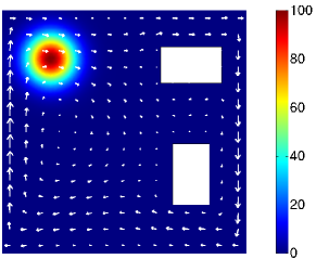
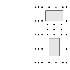
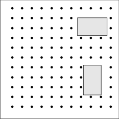
Figure 1: The domain $\mathcal{D}$ for the model problem is $[0,1]^{2}$ with the two rectangular regions removed (left); we show the “true” initial state and the arrows indicate the velocity field. Two possible grid of candidate sensor locations (middle, right).

The observation operator denoted by $\mathcal{B}$, returns the values of the state variable $u$ at a set of sensor locations $\{{\mathchoice{\mbox{\boldmath$\displaystyle{x}$}}{\mbox{\boldmath$\textstyle{x}$}}{\mbox{\boldmath$\scriptstyle{x}$}}{\mbox{\boldmath$\scriptscriptstyle{x}$}}}_{1},\ldots,{\mathchoice{\mbox{\boldmath$\displaystyle{x}$}}{\mbox{\boldmath$\textstyle{x}$}}{\mbox{\boldmath$\scriptstyle{x}$}}{\mbox{\boldmath$\scriptscriptstyle{x}$}}}_{n_{s}}\}\subset\mathcal{D}$ at observation times $\{t_{1},\ldots,t_{n_{t}}\}\subset[0,T]$. Hence, an evaluation of the parameter-to-observable map, denoted by $F$ in the infinite dimensions, involves, first solving the time-dependent advection-diffusion equation (39) to obtain $u=u(\theta)$, and then applying the observation operator that returns value of $u$ at the measurement locations and times. That is, ${F}\theta={\mathchoice{\mbox{\boldmath$\displaystyle{y}$}}{\mbox{\boldmath$\textstyle{y}$}}{\mbox{\boldmath$\scriptstyle{y}$}}{\mbox{\boldmath$\scriptscriptstyle{y}$}}}$, where ${\mathchoice{\mbox{\boldmath$\displaystyle{y}$}}{\mbox{\boldmath$\textstyle{y}$}}{\mbox{\boldmath$\scriptstyle{y}$}}{\mbox{\boldmath$\scriptscriptstyle{y}$}}}\in\mathbb{R}^{n_{y}}$ is given by, ${\mathchoice{\mbox{\boldmath$\displaystyle{y}$}}{\mbox{\boldmath$\textstyle{y}$}}{\mbox{\boldmath$\scriptstyle{y}$}}{\mbox{\boldmath$\scriptscriptstyle{y}$}}}=[{\mathchoice{\mbox{\boldmath$\displaystyle{y}$}}{\mbox{\boldmath$\textstyle{y}$}}{\mbox{\boldmath$\scriptstyle{y}$}}{\mbox{\boldmath$\scriptscriptstyle{y}$}}}_{1}^{\mkern-1.5mu\mathsf{T}},{\mathchoice{\mbox{\boldmath$\displaystyle{y}$}}{\mbox{\boldmath$\textstyle{y}$}}{\mbox{\boldmath$\scriptstyle{y}$}}{\mbox{\boldmath$\scriptscriptstyle{y}$}}}_{2}^{\mkern-1.5mu\mathsf{T}},\ldots,{\mathchoice{\mbox{\boldmath$\displaystyle{y}$}}{\mbox{\boldmath$\textstyle{y}$}}{\mbox{\boldmath$\scriptstyle{y}$}}{\mbox{\boldmath$\scriptscriptstyle{y}$}}}_{n_{t}}^{\mkern-1.5mu\mathsf{T}}]^{\mkern-1.5mu\mathsf{T}}$, where $y_{j}^{i}$ is the value of $u$ at ${\mathchoice{\mbox{\boldmath$\displaystyle{x}$}}{\mbox{\boldmath$\textstyle{x}$}}{\mbox{\boldmath$\scriptstyle{x}$}}{\mbox{\boldmath$\scriptscriptstyle{x}$}}}_{i}$ and at observation time $t_{j}$.

In what follows, we also need the action of the adjoint ${F}^{*}$ of the parameter-to-observable map ${F}$ to vectors. For a given observation vector $\bar{{\mathchoice{\mbox{\boldmath$\displaystyle{y}$}}{\mbox{\boldmath$\textstyle{y}$}}{\mbox{\boldmath$\scriptstyle{y}$}}{\mbox{\boldmath$\scriptscriptstyle{y}$}}}}\in\mathbb{R}^{n_{y}}$, ${F}^{*}\bar{{\mathchoice{\mbox{\boldmath$\displaystyle{y}$}}{\mbox{\boldmath$\textstyle{y}$}}{\mbox{\boldmath$\scriptstyle{y}$}}{\mbox{\boldmath$\scriptscriptstyle{y}$}}}}$ is computed by solving the adjoint equation (see [1, 19, 35]) for the adjoint variable $p=p({\mathchoice{\mbox{\boldmath$\displaystyle{x}$}}{\mbox{\boldmath$\textstyle{x}$}}{\mbox{\boldmath$\scriptstyle{x}$}}{\mbox{\boldmath$\scriptscriptstyle{x}$}}},t)$,

(40) $$-p_{t}-\nabla\cdot(p{\mathchoice{\mbox{\boldmath$\displaystyle{v}$}}{\mbox{\boldmath$\textstyle{v}$}}{\mbox{\boldmath$\scriptstyle{v}$}}{\mbox{\boldmath$\scriptscriptstyle{v}$}}})-\kappa\Delta p =-\mathcal{B}^{*}\bar{{\mathchoice{\mbox{\boldmath$\displaystyle{y}$}}{\mbox{\boldmath$\textstyle{y}$}}{\mbox{\boldmath$\scriptstyle{y}$}}{\mbox{\boldmath$\scriptscriptstyle{y}$}}}} \text{ in }\mathcal{D}\times(0,T),$$

$$p(\cdot,T) =0 \text{ in }\mathcal{D},$$

$$({\mathchoice{\mbox{\boldmath$\displaystyle{v}$}}{\mbox{\boldmath$\textstyle{v}$}}{\mbox{\boldmath$\scriptstyle{v}$}}{\mbox{\boldmath$\scriptscriptstyle{v}$}}}p+\kappa\nabla p)\cdot{\mathchoice{\mbox{\boldmath$\displaystyle{n}$}}{\mbox{\boldmath$\textstyle{n}$}}{\mbox{\boldmath$\scriptstyle{n}$}}{\mbox{\boldmath$\scriptscriptstyle{n}$}}} =0 \text{ on }\partial\mathcal{D}\times(0,T),$$

and setting ${F}^{*}\bar{{\mathchoice{\mbox{\boldmath$\displaystyle{y}$}}{\mbox{\boldmath$\textstyle{y}$}}{\mbox{\boldmath$\scriptstyle{y}$}}{\mbox{\boldmath$\scriptscriptstyle{y}$}}}}=-p(\cdot,0)$. Note that this equation is a final value problem that is solved backwards in time.

Bayesian inverse problem formulation

The Bayesian inverse problem seeks to infer the initial state $\theta$ from point measurements of $u$. Following the setup outlined in section 2, we utilize a Gaussian prior measure $\mu_{\text{pr}}=\mathcal{N}\!\left({\theta_{\mathup{pr}}},{\mathcal{C}_{\mathup{pr}}}\right)$, with $\mathcal{C}_{\mathup{pr}}$ as described before, and use an additive Gaussian noise model. Specifically, we use $\alpha=2\times 10^{-3}$ and $\beta=10^{-1}$ in (6). The “true” initial state shown in Figure 1(left) is used to synthesize data, and the noise level is set as follows. We solve the forward model using the true initial state and record measurements of the state at the candidate sensor locations and at the observation times (see numerical results section for specifics), and define the noise level as two percent of the maximum of the recorded measurements.

Discretization

We discretize the forward and adjoint problems via linear triangular continuous Galerkin finite elements in the two-dimensional spatial domain, and use the implicit Euler method for time integration. As in [35, 3], we follow a discretize-then-optimize approach, where the discrete adjoint equation is obtained as the adjoint of the discretized forward equation.

6 Numerical results

In this section, we test various aspects of our proposed numerical methods for D-optimal sensor placement. Section 6.1 is devoted to testing accuracy of our randomized estimators, and a simple illustration of D-optimal sensor placements using the randomized approach. In section 6.2 we consider a more realistic example in which we allow a denser grid of candidate sensor locations, and the unknown parameters are discretized on a grid of higher resolution. The D-optimal sensor placement methods are illustrated on this application.

6.1 Test of accuracy and basic illustrations

In this subsection, we use the following parameters that specify the test problem: we pick the grid of $n_{s}=35$ candidate sensor locations, depicted in Figure 1 (middle), with $n_{t}=3$ observation times given by $t=1$, $t=2$, $t=3.5$, for a total of $105$ observations. The discretized parameter dimension for this example is ${n}=1018$.

Accuracy of KL-divergence estimator

Here we demonstrate the accuracy of the estimators for the computation of the Kullback-Liebler divergence. We take $\textstyle{w}$ to be a $35\times 1$ vector of all ones; i.e., all the sensors are active.

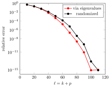
Figure 2: Accuracy of KL divergence estimators  (21) (exact eigenvalues) and  (24) (randomized).

We estimate the KL divergence using two different methods proposed in section 4.1. In the first method the KL divergence is computed using “exact” eigenvalues (21); the approximation is because only $k\leq K$ eigenvalues are used for estimating the KL divergence. The “exact” eigenvalues were computed using eigs function in MATLAB. In the second method we compute the KL divergence using the randomized estimator (24). The oversampling parameter was fixed to be $p=5$, we increase the total number of random samples $\ell=k+p$ between $20$ and $105$; since the oversampling parameter is fixed, this amounts to increasing the target rank $k$. The error in the KL divergence is plotted in Figure 2. As we see, the error decays rapidly as the number of computed eigenvalue increases, and the randomized estimators is nearly as accurate as using the “exact” eigenvalues, but is, in general, considerably more efficient to compute.

Accuracy of D-optimal criterion and its derivative

The setup is the same as the previous experiment; now, we consider the accuracy of the D-optimal objective function and the gradient. We use Eig-$k$ and randomized estimators and the results are plotted in Figure 3 (left, middle). Similar conclusions are drawn here as well: the error decreases with increasing target rank $k$ and the accuracy of the randomized estimators is comparable with that of Eig-$k$. Note that since we used $\bm{\mathrm{W}}=\bm{\mathrm{I}}$, the frozen and Eig-$k$ approaches are essentially equivalent, for the present test. In our next experiment, we plot the accuracy of the objective function as a function of mesh refinement in Figure 3 (right). The accuracy of the estimators does not degrade with increasing mesh refinement. This desirable property is also a numerical illustration of the fact that our formulation remains valid in the infinite-dimensional limit.

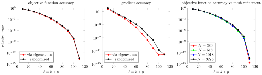
Figure 3: The relative error in the D-optimal objective function (left) and relative error in the $2$-norm of the gradient (center). Performance of randomized estimator with mesh refinement (right).

Computing D-optimal designs

We have demonstrated that our estimators are accurate; we now show how the corresponding designs look like. As a first illustration, we use the randomized approach in section 4.2.2, where OED objective and gradient are computed according Algorithm 3, to compute a D-optimal sensor placement. The $\ell_{1}$-norm is chosen as the penalty function to ensure sparsification (see section 4.3). The resulting design has weights between $0$ and $1$. To enforce binary weights, the following thresholding criterion was used: if the sensor weight $w_{i}$ satisfies $w_{i}/\sum_{j}w_{j}\geq 3\times 10^{-2}$ then it is set to be $1$ else $0$. The resulting designs are plotted in Figure 4 (left). We also plot the relative errors in objective and gradient computations during the course of the optimization iteration history in Figure 4 (right). The latter shows that the randomized estimators remain accurate over the course of the iterations.

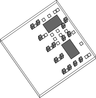
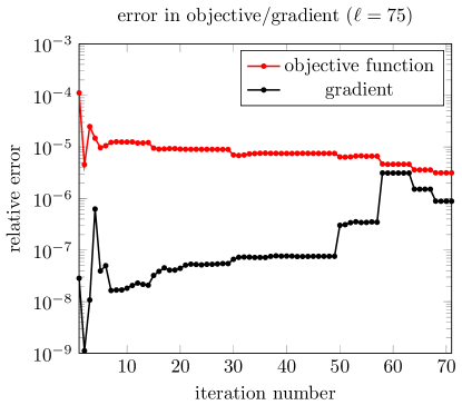
Figure 4: Left: D-optimal design with $15$ active sensors; the sensor placement was obtained using an $\ell_{1}$-norm penalty approach, with penalty parameter $\gamma=9$. Sensors are placed at locations whose corresponding sensor weight exceeded $w_{i}/\sum_{j}w_{j}\geq 3\times 10^{-2}$. Right: relative error in OED objective and gradient over optimization iterations.

To compare the different methods proposed in the present work, we compute optimal design weights using spectral, randomized, and frozen low-rank approaches; see Figure 5. To remain consistent across methods, for each method we use rank $k=70$ approximations with an oversampling parameter of $p=5$. We use a log-scale on the vertical axis, and plot the computed weights in descending order; reported also are the respective optimal objective values. As expected, the randomized and spectral approaches lead to nearly identical optimal weights; on the other hand, the solution obtained via the frozen approach, agree with that of the randomized and spectral approach only for the larger weights.

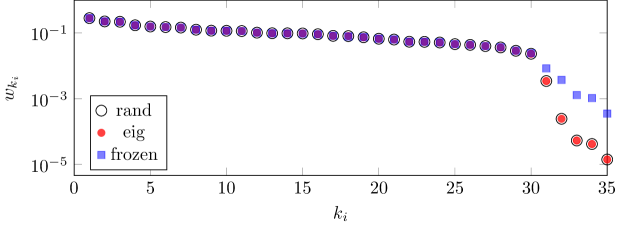
Figure 5: Comparing the optimal design weights obtained using the randomized, spectral, and frozen low-rank approaches; the objective value at the respective solutions were $-72.5847$, $-72.5848$, $-72.5786$. The problems were solved with an $\ell_{1}$-norm penalty and a penalty parameter of $\gamma=9$.

6.2 A higher resolution example

Here we illustrate computing a D-optimal sensor placement on a problem with parameter dimension $n=2605$, and a grid of ${n_{s}}=109$ candidate sensor locations; see Figure 1(right). To enforce binary weights, we used the continuation approach described in section 4.3. We picked the penalty parameter $\gamma=1.8$ and the penalty functions $P_{\varepsilon}$ is as in [3, Section 4.5]. We use six continuation steps with $\{P_{\varepsilon_{i}}\}_{i=1}^{n_{\text{cont}}}$, $\varepsilon_{i}=1/2^{i}$. The resulting D-optimal sensor placement is shown in Figure 6 (left) and the convergence of the successive design vectors to a binary weight vector is shown in Figure 6 (right).

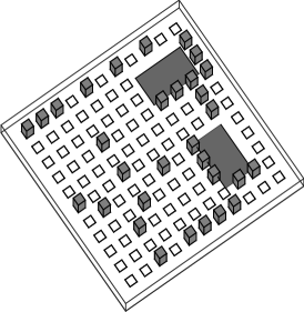
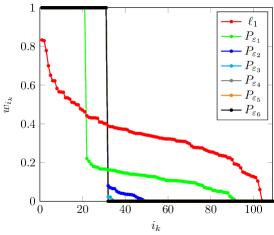
Figure 6: Left: a D-optimal design computed on the resolution model problem; right: the design weights, sorted in descending order, during the continuation.

Testing the effectiveness of the computed D-optimal design

We illustrate the effectiveness of the computed D-optimal sensor placement by comparing it with an ensemble of randomly generated sensor placements. Since the continuation approach yielded $31$ active sensors, the random sensor placements had the same number of sensors. For each design (random ones and the optimal one), we compute the objective value ${J}({\mathchoice{\mbox{\boldmath$\displaystyle{w}$}}{\mbox{\boldmath$\textstyle{w}$}}{\mbox{\boldmath$\scriptstyle{w}$}}{\mbox{\boldmath$\scriptscriptstyle{w}$}}})$, as well as the KL divergence from the posterior to prior. To compute the KL divergence, the inverse problem was solved for each of the sensor placements and the randomized estimator (24) was used.

In the first place, it is expected that the computed optimal design outperform random designs in terms of smaller OED objective value. Moreover, Theorem 3.1 indicates that maximizing ${J}({\mathchoice{\mbox{\boldmath$\displaystyle{w}$}}{\mbox{\boldmath$\textstyle{w}$}}{\mbox{\boldmath$\scriptstyle{w}$}}{\mbox{\boldmath$\scriptscriptstyle{w}$}}})$ results in maximizing the expected information gain. Both of these issues are illustrated in Figure 7. The red dots in that figure correspond to $500$ randomly generated sensor configurations with $31$ sensors and the black dot to the computed optimal design. That the black dot falls below all the red dots is to be expected, because the quantity in the vertical axis, $-J({\mathchoice{\mbox{\boldmath$\displaystyle{w}$}}{\mbox{\boldmath$\textstyle{w}$}}{\mbox{\boldmath$\scriptstyle{w}$}}{\mbox{\boldmath$\scriptscriptstyle{w}$}}})=-\log\det(\bm{\mathrm{I}}+\boldsymbol{\mathcal{H}}{m}({\mathchoice{\mbox{\boldmath$\displaystyle{w}$}}{\mbox{\boldmath$\textstyle{w}$}}{\mbox{\boldmath$\scriptstyle{w}$}}{\mbox{\boldmath$\scriptscriptstyle{w}$}}}))$, is what we sought to minimize. On the other hand, the computed D-optimal sensor placement maximizes the information gain in the average sense specified in Theorem 3.1; this explains the location of the black dot in the horizontal axis.

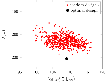
Figure 7: Comparing $-J({\mathchoice{\mbox{\boldmath$\displaystyle{w}$}}{\mbox{\boldmath$\textstyle{w}$}}{\mbox{\boldmath$\scriptstyle{w}$}}{\mbox{\boldmath$\scriptscriptstyle{w}$}}})=-\log\det(\bm{\mathrm{I}}+\boldsymbol{\mathcal{H}}{m}({\mathchoice{\mbox{\boldmath$\displaystyle{w}$}}{\mbox{\boldmath$\textstyle{w}$}}{\mbox{\boldmath$\scriptstyle{w}$}}{\mbox{\boldmath$\scriptscriptstyle{w}$}}}))$ and the information gain, computed at the optimal design (black dot) with $500$ randomly generated designs (red dots).

Solving the inverse problem using the computed optimal design

Finally, we report the results of solving the Bayesian inverse problem via the computed D-optimal sensor placement. Figure 8 shows the “true” parameter (initial state) and the computed MAP estimator. Figure 9 (top) compares the prior and posterior standard deviation fields, showing reduction in uncertainty and the information gain by using an optimal sensor placement. Figure 9 (bottom) shows three samples drawn from the posterior distribution.

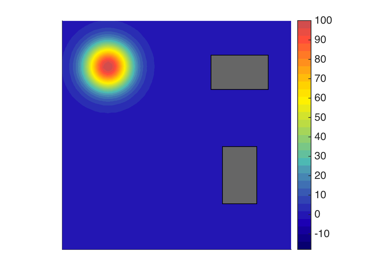
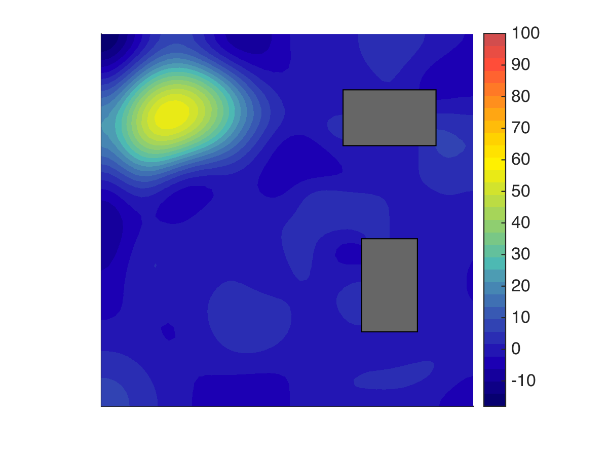
Figure 8: The true parameter (left) and the MAP estimator (right).

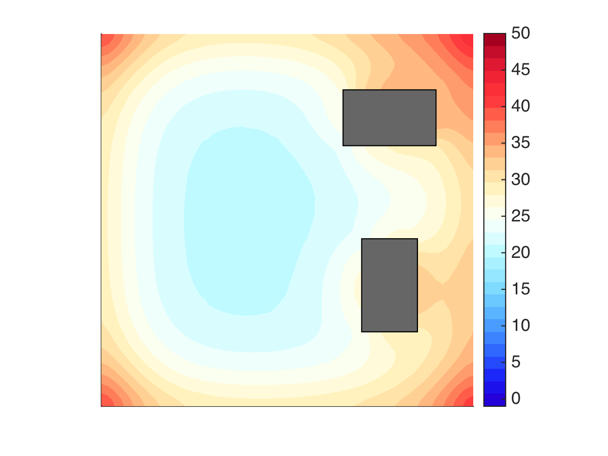
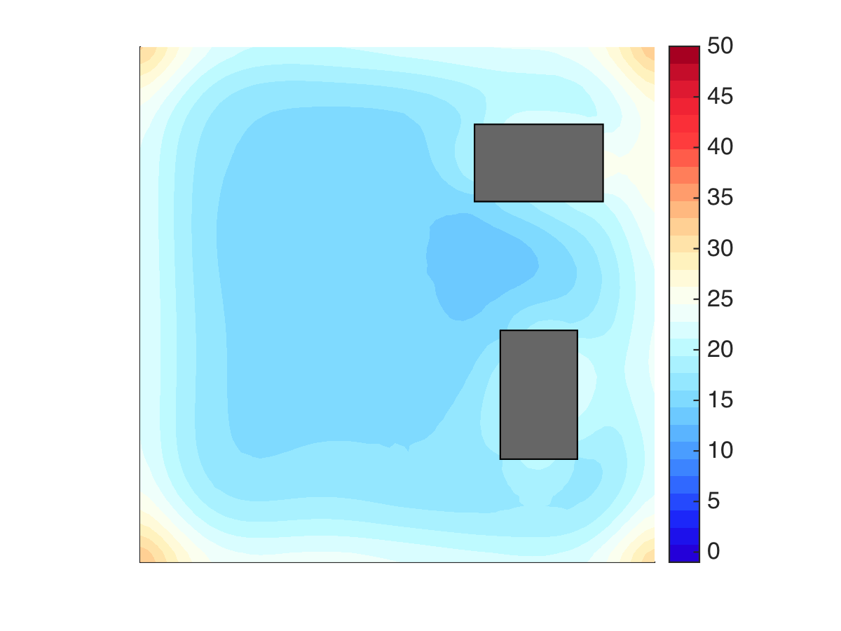
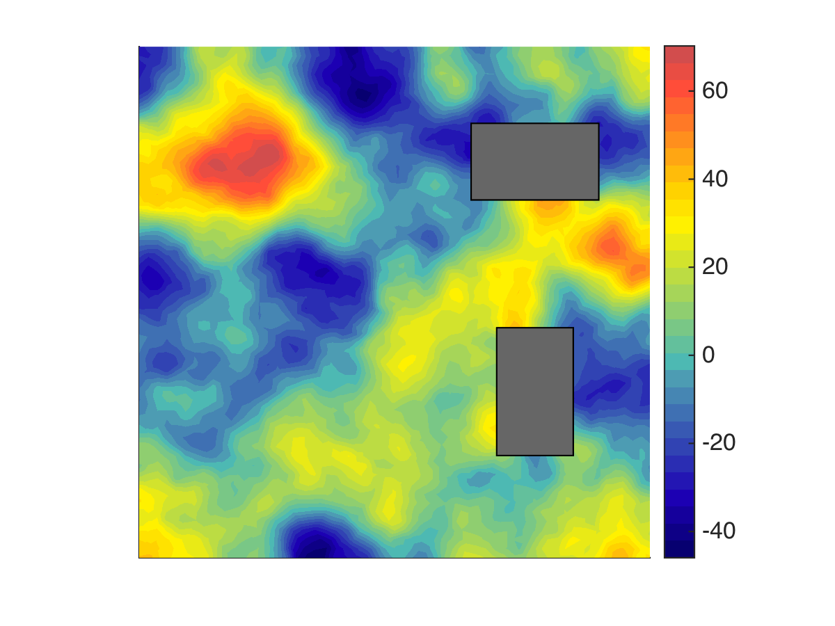
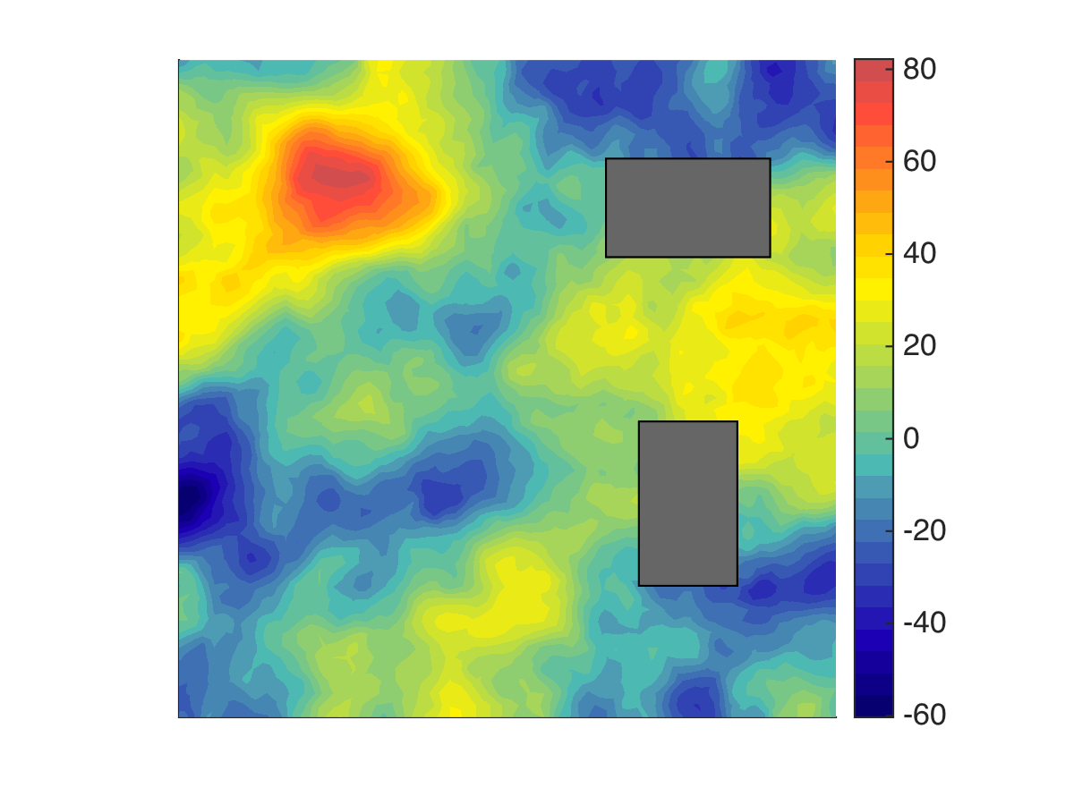
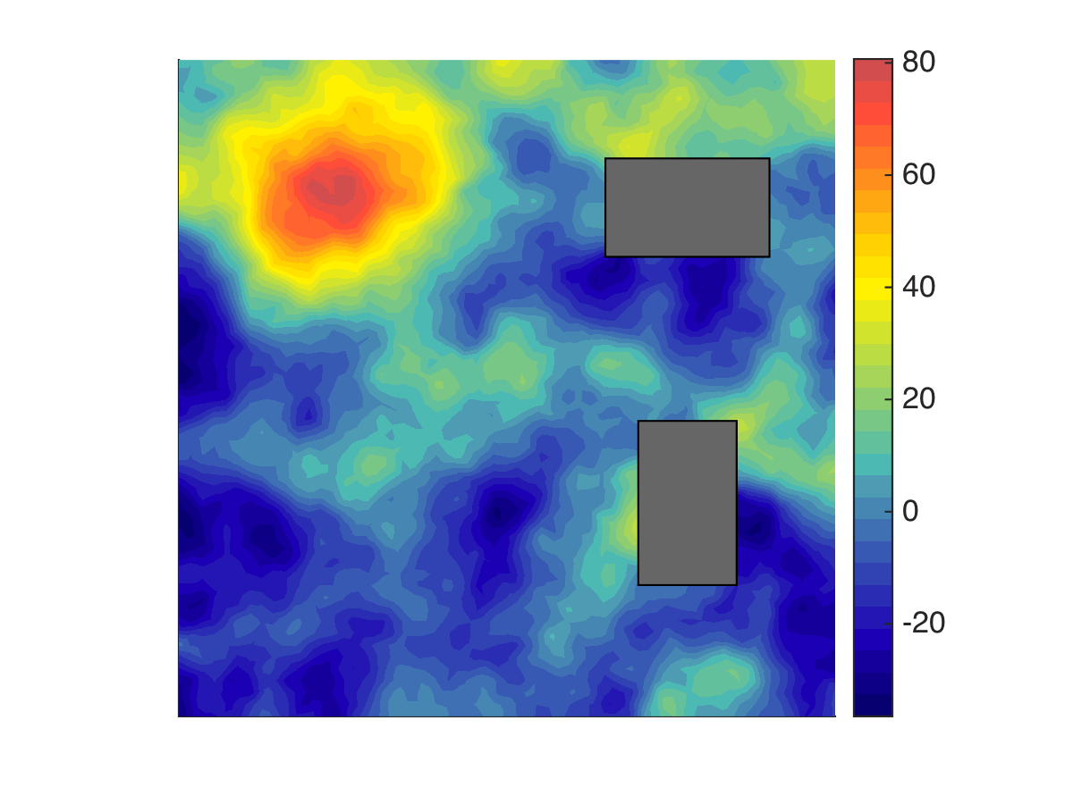
Figure 9: The prior (left) and posterior (right) standard deviation fields.

7 Conclusion

We have developed a computational framework for D-optimal experimental design for PDE-based Bayesian linear inverse problems with infinite-dimensional parameters. Our methods exploit low-rank structure of the prior-preconditioned data misfit Hessian, and the prior-preconditioned forward operator for fast estimation of OED objective and its gradient, as well as the KL divergence from posterior to prior. Our developments resulted in three different approaches: the low-rank spectral decomposition approach, the randomized approach, and the approach based on fixed low-rank SVD of the prior-preconditioned forward operator. Our numerical results, aiming at D-optimal sensor placement for initial state inversion in a time-dependent advection-diffusion equation, demonstrate the effectiveness of our methods.

The randomized and spectral approaches provide accurate and efficient estimators of the OED objective and gradient; the accuracy is controlled by setting the target rank $k$, which is specified a priori. Some open questions remain: can we adaptively determine the target rank $k$ during the optimization iterations so as to ensure the objective function and the gradient are accurate to a given tolerance, with as few PDE solves as necessary? Can suitable error estimators be incorporated into an optimization routine with theoretical guarantees of convergence? Can the presented strategy be extended to OED for nonlinear inverse problems? Addressing these questions is subject of our future work.

Appendix A Proofs

A.1 Proof of Theorem 3.1

We define the operator $\bm{\mathrm{S}}=(\boldsymbol{\mathcal{H}}{m}+\bm{\mathrm{I}})^{-1}$. Using the definition of $\bm{\theta}_{\text{post}}^{\mathchoice{\mbox{\boldmath$\displaystyle{y}$}}{\mbox{\boldmath$\textstyle{y}$}}{\mbox{\boldmath$\scriptstyle{y}$}}{\mbox{\boldmath$\scriptscriptstyle{y}$}}}$ we have,

$$\operatorname{E}_{{{\mathchoice{\mbox{\boldmath$\displaystyle{y}$}}{\mbox{\boldmath$\textstyle{y}$}}{\mbox{\boldmath$\scriptstyle{y}$}}{\mbox{\boldmath$\scriptscriptstyle{y}$}}}|\bm{\theta}}}\left\{{\left\langle{\bm{\theta}_{\text{post}}^{\mathchoice{\mbox{\boldmath$\displaystyle{y}$}}{\mbox{\boldmath$\textstyle{y}$}}{\mbox{\boldmath$\scriptstyle{y}$}}{\mbox{\boldmath$\scriptscriptstyle{y}$}}}},{\bm{\theta}_{\text{post}}^{\mathchoice{\mbox{\boldmath$\displaystyle{y}$}}{\mbox{\boldmath$\textstyle{y}$}}{\mbox{\boldmath$\scriptstyle{y}$}}{\mbox{\boldmath$\scriptscriptstyle{y}$}}}}\right\rangle_{\!\bm{\Gamma}_{\mathup{prior}}^{-1}}}\right\} =\operatorname{E}_{{{\mathchoice{\mbox{\boldmath$\displaystyle{y}$}}{\mbox{\boldmath$\textstyle{y}$}}{\mbox{\boldmath$\scriptstyle{y}$}}{\mbox{\boldmath$\scriptscriptstyle{y}$}}}|\bm{\theta}}}\left\{{\left\langle{\bm{\mathrm{\Gamma}}_{\text{post}}\bm{\mathrm{F}}^{*}{\mathchoice{\mbox{\boldmath$\displaystyle{\Gamma}$}}{\mbox{\boldmath$\textstyle{\Gamma}$}}{\mbox{\boldmath$\scriptstyle{\Gamma}$}}{\mbox{\boldmath$\scriptscriptstyle{\Gamma}$}}}_{\!\mathup{noise}}^{-1}{\mathchoice{\mbox{\boldmath$\displaystyle{y}$}}{\mbox{\boldmath$\textstyle{y}$}}{\mbox{\boldmath$\scriptstyle{y}$}}{\mbox{\boldmath$\scriptscriptstyle{y}$}}}},{\bm{\Gamma}_{\mathup{prior}}^{-1}(\bm{\mathrm{\Gamma}}_{\text{post}}\bm{\mathrm{F}}^{*}{\mathchoice{\mbox{\boldmath$\displaystyle{\Gamma}$}}{\mbox{\boldmath$\textstyle{\Gamma}$}}{\mbox{\boldmath$\scriptstyle{\Gamma}$}}{\mbox{\boldmath$\scriptscriptstyle{\Gamma}$}}}_{\!\mathup{noise}}^{-1}{\mathchoice{\mbox{\boldmath$\displaystyle{y}$}}{\mbox{\boldmath$\textstyle{y}$}}{\mbox{\boldmath$\scriptstyle{y}$}}{\mbox{\boldmath$\scriptscriptstyle{y}$}}})}\right\rangle_{\!\scriptscriptstyle{\bm{M}}}}\right\}$$

$$=\operatorname{E}_{{{\mathchoice{\mbox{\boldmath$\displaystyle{y}$}}{\mbox{\boldmath$\textstyle{y}$}}{\mbox{\boldmath$\scriptstyle{y}$}}{\mbox{\boldmath$\scriptscriptstyle{y}$}}}|\bm{\theta}}}\left\{{\left\langle{{\mathchoice{\mbox{\boldmath$\displaystyle{y}$}}{\mbox{\boldmath$\textstyle{y}$}}{\mbox{\boldmath$\scriptstyle{y}$}}{\mbox{\boldmath$\scriptscriptstyle{y}$}}}},{{\mathchoice{\mbox{\boldmath$\displaystyle{\Gamma}$}}{\mbox{\boldmath$\textstyle{\Gamma}$}}{\mbox{\boldmath$\scriptstyle{\Gamma}$}}{\mbox{\boldmath$\scriptscriptstyle{\Gamma}$}}}_{\!\mathup{noise}}^{-1}\bm{\mathrm{F}}\bm{\mathrm{\Gamma}}_{\text{post}}\bm{\Gamma}_{\mathup{prior}}^{-1}\bm{\mathrm{\Gamma}}_{\text{post}}\bm{\mathrm{F}}^{*}{\mathchoice{\mbox{\boldmath$\displaystyle{\Gamma}$}}{\mbox{\boldmath$\textstyle{\Gamma}$}}{\mbox{\boldmath$\scriptstyle{\Gamma}$}}{\mbox{\boldmath$\scriptscriptstyle{\Gamma}$}}}_{\!\mathup{noise}}^{-1}{\mathchoice{\mbox{\boldmath$\displaystyle{y}$}}{\mbox{\boldmath$\textstyle{y}$}}{\mbox{\boldmath$\scriptstyle{y}$}}{\mbox{\boldmath$\scriptscriptstyle{y}$}}}}\right\rangle}\right\}$$

$$=\operatorname{E}_{{{\mathchoice{\mbox{\boldmath$\displaystyle{y}$}}{\mbox{\boldmath$\textstyle{y}$}}{\mbox{\boldmath$\scriptstyle{y}$}}{\mbox{\boldmath$\scriptscriptstyle{y}$}}}|\bm{\theta}}}\left\{{\left\langle{{\mathchoice{\mbox{\boldmath$\displaystyle{y}$}}{\mbox{\boldmath$\textstyle{y}$}}{\mbox{\boldmath$\scriptstyle{y}$}}{\mbox{\boldmath$\scriptscriptstyle{y}$}}}},{{\mathchoice{\mbox{\boldmath$\displaystyle{\Gamma}$}}{\mbox{\boldmath$\textstyle{\Gamma}$}}{\mbox{\boldmath$\scriptstyle{\Gamma}$}}{\mbox{\boldmath$\scriptscriptstyle{\Gamma}$}}}_{\!\mathup{noise}}^{-1}\bm{\mathrm{F}}\bm{\Gamma}_{\mathup{prior}}^{1/2}\bm{\mathrm{S}}^{2}\bm{\Gamma}_{\mathup{prior}}^{1/2}\bm{\mathrm{F}}^{*}{\mathchoice{\mbox{\boldmath$\displaystyle{\Gamma}$}}{\mbox{\boldmath$\textstyle{\Gamma}$}}{\mbox{\boldmath$\scriptstyle{\Gamma}$}}{\mbox{\boldmath$\scriptscriptstyle{\Gamma}$}}}_{\!\mathup{noise}}^{-1}{\mathchoice{\mbox{\boldmath$\displaystyle{y}$}}{\mbox{\boldmath$\textstyle{y}$}}{\mbox{\boldmath$\scriptstyle{y}$}}{\mbox{\boldmath$\scriptscriptstyle{y}$}}}}\right\rangle}\right\},$$

where we have used that $\bm{\mathrm{\Gamma}}_{\text{post}}=\bm{\Gamma}_{\mathup{prior}}^{1/2}\bm{\mathrm{S}}\bm{\Gamma}_{\mathup{prior}}^{1/2}$ in the last step. Due to our choice of the noise model, ${\mathchoice{\mbox{\boldmath$\displaystyle{y}$}}{\mbox{\boldmath$\textstyle{y}$}}{\mbox{\boldmath$\scriptstyle{y}$}}{\mbox{\boldmath$\scriptscriptstyle{y}$}}}|\bm{\theta}\sim\mathcal{N}\!\left({\bm{\mathrm{F}}\bm{\theta}},{{\mathchoice{\mbox{\boldmath$\displaystyle{\Gamma}$}}{\mbox{\boldmath$\textstyle{\Gamma}$}}{\mbox{\boldmath$\scriptstyle{\Gamma}$}}{\mbox{\boldmath$\scriptscriptstyle{\Gamma}$}}}_{\!\mathup{noise}}}\right)$, therefore, by the formula for the expectation of a quadratic form we have,

(41) $$\operatorname{E}_{{{\mathchoice{\mbox{\boldmath$\displaystyle{y}$}}{\mbox{\boldmath$\textstyle{y}$}}{\mbox{\boldmath$\scriptstyle{y}$}}{\mbox{\boldmath$\scriptscriptstyle{y}$}}}|\bm{\theta}}}\left\{{\left\langle{\bm{\theta}_{\text{post}}^{\mathchoice{\mbox{\boldmath$\displaystyle{y}$}}{\mbox{\boldmath$\textstyle{y}$}}{\mbox{\boldmath$\scriptstyle{y}$}}{\mbox{\boldmath$\scriptscriptstyle{y}$}}}},{\bm{\theta}_{\text{post}}^{\mathchoice{\mbox{\boldmath$\displaystyle{y}$}}{\mbox{\boldmath$\textstyle{y}$}}{\mbox{\boldmath$\scriptstyle{y}$}}{\mbox{\boldmath$\scriptscriptstyle{y}$}}}}\right\rangle_{\!\bm{\Gamma}_{\mathup{prior}}^{-1}}}\right\}=$$

$$\quad\mathsf{tr}\,({\mathchoice{\mbox{\boldmath$\displaystyle{\Gamma}$}}{\mbox{\boldmath$\textstyle{\Gamma}$}}{\mbox{\boldmath$\scriptstyle{\Gamma}$}}{\mbox{\boldmath$\scriptscriptstyle{\Gamma}$}}}_{\!\mathup{noise}}^{-1}\bm{\mathrm{F}}\bm{\Gamma}_{\mathup{prior}}^{1/2}\bm{\mathrm{S}}^{2}\bm{\Gamma}_{\mathup{prior}}^{1/2}\bm{\mathrm{F}}^{*})+\left\langle{\bm{\mathrm{F}}\bm{\theta}},{{\mathchoice{\mbox{\boldmath$\displaystyle{\Gamma}$}}{\mbox{\boldmath$\textstyle{\Gamma}$}}{\mbox{\boldmath$\scriptstyle{\Gamma}$}}{\mbox{\boldmath$\scriptscriptstyle{\Gamma}$}}}_{\!\mathup{noise}}^{-1}\bm{\mathrm{F}}\bm{\Gamma}_{\mathup{prior}}^{1/2}\bm{\mathrm{S}}^{2}\bm{\Gamma}_{\mathup{prior}}^{1/2}\bm{\mathrm{F}}^{*}{\mathchoice{\mbox{\boldmath$\displaystyle{\Gamma}$}}{\mbox{\boldmath$\textstyle{\Gamma}$}}{\mbox{\boldmath$\scriptstyle{\Gamma}$}}{\mbox{\boldmath$\scriptscriptstyle{\Gamma}$}}}_{\!\mathup{noise}}^{-1}\bm{\mathrm{F}}\bm{\theta}}\right\rangle.$$

Now, the first term, involving the trace, simplifies as follows,

(42) $$\mathsf{tr}\,({\mathchoice{\mbox{\boldmath$\displaystyle{\Gamma}$}}{\mbox{\boldmath$\textstyle{\Gamma}$}}{\mbox{\boldmath$\scriptstyle{\Gamma}$}}{\mbox{\boldmath$\scriptscriptstyle{\Gamma}$}}}_{\!\mathup{noise}}^{-1}\bm{\mathrm{F}}\bm{\Gamma}_{\mathup{prior}}^{1/2}\bm{\mathrm{S}}^{2}\bm{\Gamma}_{\mathup{prior}}^{1/2}\bm{\mathrm{F}}^{*})=\mathsf{tr}\,(\bm{\Gamma}_{\mathup{prior}}^{1/2}\bm{\mathrm{S}}^{2}\bm{\Gamma}_{\mathup{prior}}^{1/2}\bm{\mathrm{F}}^{*}{\mathchoice{\mbox{\boldmath$\displaystyle{\Gamma}$}}{\mbox{\boldmath$\textstyle{\Gamma}$}}{\mbox{\boldmath$\scriptstyle{\Gamma}$}}{\mbox{\boldmath$\scriptscriptstyle{\Gamma}$}}}_{\!\mathup{noise}}^{-1}\bm{\mathrm{F}})=\mathsf{tr}\,(\bm{\mathrm{S}}^{2}\boldsymbol{\mathcal{H}}{m}).$$

Next, we consider the second term in (41), which we average over the prior measure:

$$\operatorname{E}_{\mu_{\text{pr}}}\left\{{\left\langle{\bm{\mathrm{F}}\bm{\theta}},{{\mathchoice{\mbox{\boldmath$\displaystyle{\Gamma}$}}{\mbox{\boldmath$\textstyle{\Gamma}$}}{\mbox{\boldmath$\scriptstyle{\Gamma}$}}{\mbox{\boldmath$\scriptscriptstyle{\Gamma}$}}}_{\!\mathup{noise}}^{-1}\bm{\mathrm{F}}\bm{\Gamma}_{\mathup{prior}}^{1/2}\bm{\mathrm{S}}^{2}\bm{\Gamma}_{\mathup{prior}}^{1/2}\bm{\mathrm{F}}^{*}{\mathchoice{\mbox{\boldmath$\displaystyle{\Gamma}$}}{\mbox{\boldmath$\textstyle{\Gamma}$}}{\mbox{\boldmath$\scriptstyle{\Gamma}$}}{\mbox{\boldmath$\scriptscriptstyle{\Gamma}$}}}_{\!\mathup{noise}}^{-1}\bm{\mathrm{F}}\bm{\theta}}\right\rangle}\right\} =\operatorname{E}_{\mu_{\text{pr}}}\left\{{\left\langle{\bm{\theta}},{\bm{\mathrm{F}}{\mathchoice{\mbox{\boldmath$\displaystyle{\Gamma}$}}{\mbox{\boldmath$\textstyle{\Gamma}$}}{\mbox{\boldmath$\scriptstyle{\Gamma}$}}{\mbox{\boldmath$\scriptscriptstyle{\Gamma}$}}}_{\!\mathup{noise}}^{-1}\bm{\mathrm{F}}\bm{\Gamma}_{\mathup{prior}}^{1/2}\bm{\mathrm{S}}^{2}\bm{\Gamma}_{\mathup{prior}}^{1/2}\bm{\mathrm{F}}^{*}{\mathchoice{\mbox{\boldmath$\displaystyle{\Gamma}$}}{\mbox{\boldmath$\textstyle{\Gamma}$}}{\mbox{\boldmath$\scriptstyle{\Gamma}$}}{\mbox{\boldmath$\scriptscriptstyle{\Gamma}$}}}_{\!\mathup{noise}}^{-1}\bm{\mathrm{F}}\bm{\theta}}\right\rangle_{\!\scriptscriptstyle{\bm{M}}}}\right\}$$

$$=\operatorname{E}_{\mu_{\text{pr}}}\left\{{\left\langle{\bm{\theta}},{\bm{\mathrm{H}}_{\mathup{m}}\bm{\Gamma}_{\mathup{prior}}^{1/2}\bm{\mathrm{S}}^{2}\bm{\Gamma}_{\mathup{prior}}^{1/2}\bm{\mathrm{H}}_{\mathup{m}}\bm{\theta}}\right\rangle_{\!\scriptscriptstyle{\bm{M}}}}\right\}$$

$$=\mathsf{tr}\,(\bm{\mathrm{H}}_{\mathup{m}}\bm{\Gamma}_{\mathup{prior}}^{1/2}\bm{\mathrm{S}}^{2}\bm{\Gamma}_{\mathup{prior}}^{1/2}\bm{\mathrm{H}}_{\mathup{m}}\bm{\Gamma}_{\mathup{prior}})$$

$$=\mathsf{tr}\,(\boldsymbol{\mathcal{H}}{m}\bm{\mathrm{S}}^{2}\boldsymbol{\mathcal{H}}{m})=\mathsf{tr}\,(\bm{\mathrm{S}}^{2}\boldsymbol{\mathcal{H}}{m}^{2}).$$

This, along with (42) and (41), lead to

(43) $$\operatorname{E}_{\mu_{\text{pr}}}\left\{{\operatorname{E}_{{{\mathchoice{\mbox{\boldmath$\displaystyle{y}$}}{\mbox{\boldmath$\textstyle{y}$}}{\mbox{\boldmath$\scriptstyle{y}$}}{\mbox{\boldmath$\scriptscriptstyle{y}$}}}|\bm{\theta}}}\left\{{\displaystyle\left\langle{\bm{\theta}_{\text{post}}^{\mathchoice{\mbox{\boldmath$\displaystyle{y}$}}{\mbox{\boldmath$\textstyle{y}$}}{\mbox{\boldmath$\scriptstyle{y}$}}{\mbox{\boldmath$\scriptscriptstyle{y}$}}}},{\bm{\theta}_{\text{post}}^{\mathchoice{\mbox{\boldmath$\displaystyle{y}$}}{\mbox{\boldmath$\textstyle{y}$}}{\mbox{\boldmath$\scriptstyle{y}$}}{\mbox{\boldmath$\scriptscriptstyle{y}$}}}}\right\rangle_{\!\bm{\Gamma}_{\mathup{prior}}^{-1}}}\right\}}\right\} =\mathsf{tr}\,(\bm{\mathrm{S}}^{2}\boldsymbol{\mathcal{H}}{m}+\bm{\mathrm{S}}^{2}\boldsymbol{\mathcal{H}}{m}^{2})$$

$$=\mathsf{tr}\,\big{(}\bm{\mathrm{S}}^{2}\boldsymbol{\mathcal{H}}{m}(\bm{\mathrm{I}}+\boldsymbol{\mathcal{H}}{m})\big{)}=\mathsf{tr}\,(\bm{\mathrm{S}}^{2}\boldsymbol{\mathcal{H}}{m}\bm{\mathrm{S}}^{-1})$$

$$=\mathsf{tr}\,(\bm{\mathrm{S}}\boldsymbol{\mathcal{H}}{m})=\mathsf{tr}\,(\boldsymbol{\mathcal{H}}{m}(\boldsymbol{\mathcal{H}}{m}+\bm{\mathrm{I}})^{-1}).$$

The stated result follows by averaging (15) over the prior and noise, as in the statement of the theorem, and using (43).

A.2 Proof of Theorem 4.1

Subtracting (24) from (12), and applying the triangle inequality, we obtain

(44) $$E_{\text{KL}}\leq\>\frac{1}{2}\left[|\log\det(\bm{\mathrm{I}}+\boldsymbol{\mathbb{H}}{m})-\log\det(\bm{\mathrm{I}}+\bm{\mathrm{T}})|+|\mathsf{tr}\,(\boldsymbol{\mathbb{H}}{m}(\bm{\mathrm{I}}+\boldsymbol{\mathbb{H}}{m})^{-1})-\mathsf{tr}\,(\bm{\mathrm{T}}(\bm{\mathrm{I}}+\bm{\mathrm{T}})^{-1})|\right].$$

By linearity of expectation, we tackle each term individually. Applying [38, Theorem 1], we obtain

(45) $$\mathbb{E}_{\bm{\mathrm{\Omega}}}\!\left[|\log\det(\bm{\mathrm{I}}+\boldsymbol{\mathbb{H}}{m})-\log\det(\bm{\mathrm{I}}+\bm{\mathrm{T}})|\right]\leq\>\log\det(\bm{\mathrm{I}}+\bm{\mathrm{\Lambda}}_{2})+\log\det(\bm{\mathrm{I}}+\gamma^{2q-1}C_{\rm ge}\bm{\mathrm{\Lambda}}_{2}).$$

For the second term, label all the eigenvalues of $\boldsymbol{\mathbb{H}}{m}$ as $\{\lambda_{i}\}_{i=1}^{n}$ and all the eigenvalues of $\bm{\mathrm{T}}$ as $\{\tilde{\lambda}_{i}\}_{i=1}^{\ell}$. Then

$$\mathsf{tr}\,(\boldsymbol{\mathbb{H}}{m}(\bm{\mathrm{I}}+\boldsymbol{\mathbb{H}}{m})^{-1})-\mathsf{tr}\,(\bm{\mathrm{T}}(\bm{\mathrm{I}}+\bm{\mathrm{T}})^{-1})= \>\sum_{i=1}^{n}\frac{\lambda_{i}}{1+\lambda_{i}}-\sum_{i=1}^{\ell}\frac{\tilde{\lambda}_{i}}{1+\tilde{\lambda}_{i}}$$

$$= \>\sum_{i=1}^{\ell}\frac{\lambda_{i}-\tilde{\lambda}_{i}}{(1+\lambda_{i})(1+\tilde{\lambda}_{i})}+\sum_{i=\ell+1}^{n}\frac{\lambda_{i}}{1+\lambda_{i}}.$$

From Cauchy interlacing theorem, $\lambda_{i}\geq\tilde{\lambda}_{i}\geq 0$ (see [38, Lemma 1]) so this expression is non-negative. We have the following inequalities

(46) $$\frac{\lambda_{i}-\tilde{\lambda}_{i}}{(1+\lambda_{i})(1+\tilde{\lambda}_{i})}\leq \>\lambda_{i}-\tilde{\lambda}_{i} i=1,\dots,\ell$$

(47) $$\frac{\lambda_{i}}{1+\lambda_{i}}\leq \>\lambda_{i} i=\ell+1,\dots,n.$$

With these relations, then

$$\mathsf{tr}\,(\boldsymbol{\mathbb{H}}{m}(\bm{\mathrm{I}}+\boldsymbol{\mathbb{H}}{m})^{-1})-\mathsf{tr}\,(\bm{\mathrm{T}}(\bm{\mathrm{I}}+\bm{\mathrm{T}})^{-1})\leq\>\sum_{i=1}^{n}\lambda_{i}-\sum_{i=1}^{\ell}\tilde{\lambda}_{i}=\mathsf{tr}\,(\boldsymbol{\mathbb{H}}{m})-\mathsf{tr}\,(\bm{\mathrm{T}}).$$

Since both sides of the inequality are nonnegative, we can take absolute values. Then apply [38, Theorem 1] to obtain

(48) $$\mathbb{E}_{\bm{\mathrm{\Omega}}}\!\left[|\mathsf{tr}\,(\boldsymbol{\mathbb{H}}{m}(\bm{\mathrm{I}}+\boldsymbol{\mathbb{H}}{m})^{-1})-\mathsf{tr}\,(\bm{\mathrm{T}}(\bm{\mathrm{I}}+\bm{\mathrm{T}})^{-1})|\right]\leq\>(1+C_{\rm ge}\gamma^{2q-1})\mathsf{tr}\,(\bm{\mathrm{\Lambda}}_{2}).$$

Substitute (45) and (48) into (44) to complete the proof.

A.3 Proof of Theorems 4.3 and 4.7

First, we record the following basic lemma:

Lemma A.1.

Let $\bm{\mathrm{A}}$ be an $n\times n$ matrix and suppose $\bm{\mathrm{B}}$ is a symmetric positive semidefinite matrix. Then, we have $|\mathsf{tr}\,(\bm{\mathrm{A}}\bm{\mathrm{B}})|\leq\left\|{\bm{\mathrm{A}}}\right\|_{2}\mathsf{tr}\,(\bm{\mathrm{B}})$.

Proof A.2.

Let $\{{\mathchoice{\mbox{\boldmath$\displaystyle{e}$}}{\mbox{\boldmath$\textstyle{e}$}}{\mbox{\boldmath$\scriptstyle{e}$}}{\mbox{\boldmath$\scriptscriptstyle{e}$}}}_{j}\}_{j=1}^{n}$ be the orthonormal basis of eigenvectors of $\bm{\mathrm{B}}$ with corresponding (real, non-negative) eigenvalues) $\{\lambda_{j}\}_{j=1}^{n}$. By Cauchy-Schwartz inequality,

$$|\mathsf{tr}\,(\bm{\mathrm{A}}\bm{\mathrm{B}})|=|\sum_{j}{\left\langle{{\mathchoice{\mbox{\boldmath$\displaystyle{e}$}}{\mbox{\boldmath$\textstyle{e}$}}{\mbox{\boldmath$\scriptstyle{e}$}}{\mbox{\boldmath$\scriptscriptstyle{e}$}}}_{j}},{\bm{\mathrm{A}}\bm{\mathrm{B}}{\mathchoice{\mbox{\boldmath$\displaystyle{e}$}}{\mbox{\boldmath$\textstyle{e}$}}{\mbox{\boldmath$\scriptstyle{e}$}}{\mbox{\boldmath$\scriptscriptstyle{e}$}}}_{j}}\right\rangle}|\leq\sum_{j}\left\|{{\mathchoice{\mbox{\boldmath$\displaystyle{e}$}}{\mbox{\boldmath$\textstyle{e}$}}{\mbox{\boldmath$\scriptstyle{e}$}}{\mbox{\boldmath$\scriptscriptstyle{e}$}}}_{j}}\right\|_{2}\left\|{\bm{\mathrm{A}}}\right\|_{2}\left\|{\bm{\mathrm{B}}{\mathchoice{\mbox{\boldmath$\displaystyle{e}$}}{\mbox{\boldmath$\textstyle{e}$}}{\mbox{\boldmath$\scriptstyle{e}$}}{\mbox{\boldmath$\scriptscriptstyle{e}$}}}_{j}}\right\|_{2}=\left\|{\bm{\mathrm{A}}}\right\|_{2}\sum_{j}\lambda_{j}=\left\|{\bm{\mathrm{A}}}\right\|_{2}\mathsf{tr}\,(\bm{\mathrm{B}}).$$

Proof A.3 (Theorem 4.3).

The first statement is immediate; the second one follows from

$$|\mathsf{tr}\,((\bm{\mathrm{UDU}}^{\mkern-1.5mu\mathsf{T}})\bm{\mathrm{Z}}_{j})-\mathsf{tr}\,((\bm{\mathrm{U}}_{k}\bm{\mathrm{D}}_{k}\bm{\mathrm{U}}_{k}^{\mkern-1.5mu\mathsf{T}})\bm{\mathrm{Z}}_{j})|\leq\left\|{\bm{\mathrm{Z}}_{j}}\right\|\sum_{j=k+1}^{K}\frac{\lambda_{i}}{1+\lambda_{i}},$$

where we have abbreviated $\bm{\mathrm{Z}}_{j}\equiv\bm{\mathrm{M}}^{1/2}\boldsymbol{\mathcal{F}}^{*}\bm{\mathrm{E}}^{\sigma}_{j}\boldsymbol{\mathcal{F}}\bm{\mathrm{M}}^{-1/2}$. The inequality is justified in Lemma (A.1) in the Appendix.

Proof A.4 (Theorem 4.7).

From Lemma A.1

$$|\partial_{j}J({\mathchoice{\mbox{\boldmath$\displaystyle{w}$}}{\mbox{\boldmath$\textstyle{w}$}}{\mbox{\boldmath$\scriptstyle{w}$}}{\mbox{\boldmath$\scriptscriptstyle{w}$}}})-\widehat{\partial_{j}J}_{\text{rand}}({\mathchoice{\mbox{\boldmath$\displaystyle{w}$}}{\mbox{\boldmath$\textstyle{w}$}}{\mbox{\boldmath$\scriptstyle{w}$}}{\mbox{\boldmath$\scriptscriptstyle{w}$}}})|\>\leq\>\|\bm{\mathrm{Z}}_{j}\|_{2}|\mathsf{tr}\,(\boldsymbol{\mathbb{H}}{m}(\bm{\mathrm{I}}+\boldsymbol{\mathbb{H}}{m})^{-1})-\mathsf{tr}\,(\bm{\mathrm{T}}(\bm{\mathrm{I}}+\bm{\mathrm{T}})^{-1})|.$$

Taking expectations and use (48) to obtain the desired bound.

A.4 Proof of Theorem 4.11

Before we turn to the proof of Theorem 4.11, we present the following Lemma.

Lemma A.5.

Let $\bm{\mathrm{M}},\bm{\mathrm{N}}\in\mathbb{C}^{n\times n}$ be Hermitian positive semidefinite with $\bm{\mathrm{M}}\geq\bm{\mathrm{N}}$. Then

$$0\leq\log\det(\bm{\mathrm{I}}+\bm{\mathrm{M}})-\log\det(\bm{\mathrm{I}}+\bm{\mathrm{N}})\leq\log\det(\bm{\mathrm{I}}+\bm{\mathrm{M}}-\bm{\mathrm{N}}).$$

Proof A.6.

The inequality $\bm{\mathrm{M}}\geq\bm{\mathrm{N}}$ is to be interpreted as $\bm{\mathrm{M}}-\bm{\mathrm{N}}$ is Hermitian positive semidefinite. Write $\bm{\mathrm{X}}=(\bm{\mathrm{I}}+\bm{\mathrm{N}})^{-1/2}$. Then, by multiplicativity of determinants,

$$\log\det(\bm{\mathrm{I}}+\bm{\mathrm{M}})-\log\det(\bm{\mathrm{I}}+\bm{\mathrm{N}})=\log\det\bm{\mathrm{X}}(\bm{\mathrm{I}}+\bm{\mathrm{M}})\bm{\mathrm{X}}.$$

Write $\bm{\mathrm{M}}=\bm{\mathrm{E}}+\bm{\mathrm{N}}$, with $\bm{\mathrm{E}}=\bm{\mathrm{M}}-\bm{\mathrm{N}}$ and

$$\bm{\mathrm{X}}(\bm{\mathrm{I}}+\bm{\mathrm{M}})\bm{\mathrm{X}}=\bm{\mathrm{X}}(\bm{\mathrm{I}}+\bm{\mathrm{N}})\bm{\mathrm{X}}+\bm{\mathrm{XEX}}=\bm{\mathrm{I}}+\bm{\mathrm{XEX}}.$$

Since $\bm{\mathrm{E}}$ is hpsd, it has a well-defined square root. Note that $\bm{\mathrm{X}}$ has singular values at most $1$, and is a contraction matrix. Furthermore, the multiplicative singular value inequalities [10, page 188] imply

$$\lambda_{j}(\bm{\mathrm{XEX}})=\sigma_{j}^{2}(\bm{\mathrm{E}}^{1/2}\bm{\mathrm{X}})\leq\sigma_{j}^{2}(\bm{\mathrm{E}}^{1/2})=\lambda_{j}(\bm{\mathrm{E}})\qquad j=1,\dots,n.$$

Writing the determinant as the product of the eigenvalues

$$\det(\bm{\mathrm{I}}+\bm{\mathrm{XEX}})=\prod_{i=1}^{n}(1+\lambda_{i}(\bm{\mathrm{XEX}}))\leq\prod_{i=1}^{n}(1+\lambda_{i}(\bm{\mathrm{E}}))=\det(\bm{\mathrm{I}}+\bm{\mathrm{E}}).$$

Taking logarithms delivers the desired upper bound. The lower bound follows from the fact that since $\bm{\mathrm{E}}$ is positive semidefinite, and $\bm{\mathrm{X}}$ is Hermitian, $\bm{\mathrm{I}}+\bm{\mathrm{XEX}}\geq\bm{\mathrm{I}}$. Therefore, $\log\det(\bm{\mathrm{I}}+\bm{\mathrm{XEX}})\geq\log\det\bm{\mathrm{I}}=0$.

Proof A.7 (Theorem 4.11).

Partition the singular value decomposition as $\boldsymbol{\mathcal{F}}=\boldsymbol{\mathcal{F}}_{k}+\boldsymbol{\mathcal{F}}_{k,\perp}$, and observe

$$\boldsymbol{\mathcal{F}}\boldsymbol{\mathcal{F}}^{*}=\boldsymbol{\mathcal{F}}_{k}\boldsymbol{\mathcal{F}}_{k}^{*}+\boldsymbol{\mathcal{F}}_{k,\perp}\boldsymbol{\mathcal{F}}_{k,\perp}^{*}.$$

The determinant identity [33, Corollary 2.1] gives

(49) $$\log\det(\bm{\mathrm{I}}+\boldsymbol{\mathcal{F}}^{*}\bm{\mathrm{W}}\boldsymbol{\mathcal{F}})=\log\det(\bm{\mathrm{I}}+\bm{\mathrm{W}}^{1/2}\boldsymbol{\mathcal{F}}\boldsymbol{\mathcal{F}}^{*}\bm{\mathrm{W}}^{1/2}).$$

It can be readily verified that $\boldsymbol{\mathcal{F}}\boldsymbol{\mathcal{F}}^{*}\geq\boldsymbol{\mathcal{F}}_{k}\boldsymbol{\mathcal{F}}_{k}^{*}$; therefore, by the lower bound in Lemma A.5

$$|J({\mathchoice{\mbox{\boldmath$\displaystyle{w}$}}{\mbox{\boldmath$\textstyle{w}$}}{\mbox{\boldmath$\scriptstyle{w}$}}{\mbox{\boldmath$\scriptscriptstyle{w}$}}})-\widehat{J}_{\text{froz}}({\mathchoice{\mbox{\boldmath$\displaystyle{w}$}}{\mbox{\boldmath$\textstyle{w}$}}{\mbox{\boldmath$\scriptstyle{w}$}}{\mbox{\boldmath$\scriptscriptstyle{w}$}}})|=\log\det(\bm{\mathrm{I}}+\boldsymbol{\mathcal{F}}^{*}\bm{\mathrm{W}}\boldsymbol{\mathcal{F}})-\log\det(\bm{\mathrm{I}}+\boldsymbol{\mathcal{F}}_{k}^{*}\bm{\mathrm{W}}\boldsymbol{\mathcal{F}}_{k}).$$

Use (49) along with the upper bound of Lemma A.5

$$\log\det(\bm{\mathrm{I}}+\boldsymbol{\mathcal{F}}^{*}\bm{\mathrm{W}}\boldsymbol{\mathcal{F}})-\log\det(\bm{\mathrm{I}}+\boldsymbol{\mathcal{F}}_{k}^{*}\bm{\mathrm{W}}\boldsymbol{\mathcal{F}}_{k})\leq \>\log\det(\bm{\mathrm{I}}+\bm{\mathrm{W}}^{1/2}\boldsymbol{\mathcal{F}}_{k,\perp}\boldsymbol{\mathcal{F}}_{k,\perp}^{*}\bm{\mathrm{W}}^{1/2})$$

$$= \>\log\det(\bm{\mathrm{I}}+\boldsymbol{\mathcal{F}}_{k,\perp}^{*}\bm{\mathrm{W}}\boldsymbol{\mathcal{F}}_{k,\perp}).$$

Since the weights are at most $1$, then $\bm{\mathrm{W}}\leq\bm{\mathrm{I}}$ and

$$\log\det(\bm{\mathrm{I}}+\boldsymbol{\mathcal{F}}_{k,\perp}^{*}\bm{\mathrm{W}}\boldsymbol{\mathcal{F}}_{k,\perp})\leq\log\det(\bm{\mathrm{I}}+\boldsymbol{\mathcal{F}}_{k,\perp}^{*}\boldsymbol{\mathcal{F}}_{k,\perp})=\log\det(\bm{\mathrm{I}}+\bm{\mathrm{\Sigma}}_{2}^{2}).$$

The inequality is due to the properties of Loewner partial ordering of Hermitian matrices [25, Corollary 7.7.4]. The final equality employs the determinant identity.

References

• [1] V. Akçelik, G. Biros, A. Drăgănescu, O. Ghattas, J. Hill, and B. van Bloeman Waanders, Dynamic data-driven inversion for terascale simulations: Real-time identification of airborne contaminants, in Proceedings of SC2005, Seattle, 2005.
• [2] A. Alexanderian, P. J. Gloor, and O. Ghattas, On Bayesian A-and D-optimal experimental designs in infinite dimensions, Bayesian Analysis, 11 (2016), pp. 671–695. arXiv preprint arXiv:1408.6323.
• [3] A. Alexanderian, N. Petra, G. Stadler, and O. Ghattas, A-optimal design of experiments for infinite-dimensional Bayesian linear inverse problems with regularized $\ell_{0}$-sparsification, SIAM Journal on Scientific Computing, 36 (2014), pp. A2122–A2148.
• [4] A. Alexanderian, N. Petra, G. Stadler, and O. Ghattas, A fast and scalable method for A-optimal design of experiments for infinite-dimensional Bayesian nonlinear inverse problems, SIAM Journal on Scientific Computing, 38 (2016), pp. A243–A272.
• [5]  , Mean-variance risk-averse optimal control of systems governed by pdes with random parameter fields using quadratic approximations, SIAM/ASA Journal on Uncertainty Quantification, to appear, (2017).
• [6] A. C. Atkinson and A. N. Donev, Optimum Experimental Designs, Oxford, 1992.
• [7] H. Avron and S. Toledo, Randomized algorithms for estimating the trace of an implicit symmetric positive semi-definite matrix, Journal of the ACM (JACM), 58 (2011), p. 17.
• [8] T. Bakhos, P. K. Kitanidis, S. Ladenheim, A. K. Saibaba, and D. B. Szyld, Multipreconditioned gmres for shifted systems, SIAM Journal on Scientific Computing, 39 (2017), pp. S222–S247.
• [9] I. Bauer, H. G. Bock, S. Körkel, and J. P. Schlöder, Numerical methods for optimum experimental design in DAE systems, Journal of Computational and Applied Mathematics, 120 (2000), pp. 1–25. SQP-based direct discretization methods for practical optimal control problems.
• [10] R. Bhatia, Notes on functional analysis, vol. 50 of Texts and Readings in Mathematics, Hindustan Book Agency, New Delhi, 2009.
• [11] F. Bisetti, D. Kim, O. Knio, Q. Long, and R. Tempone, Optimal Bayesian experimental design for priors of compact support with application to shock-tube experiments for combustion kinetics, International Journal for Numerical Methods in Engineering, 108 (2016), pp. 136–155.
• [12] T. Bui-Thanh, O. Ghattas, J. Martin, and G. Stadler, A computational framework for infinite-dimensional Bayesian inverse problems Part I: The linearized case, with application to global seismic inversion, SIAM Journal on Scientific Computing, 35 (2013), pp. A2494–A2523.
• [13] K. Chaloner and I. Verdinelli, Bayesian experimental design: A review, Statistical Science, 10 (1995), pp. 273–304.
• [14] J. Chen, M. Anitescu, and Y. Saad, Computing f(a)b via least squares polynomial approximations, SIAM Journal on Scientific Computing, 33 (2011), pp. 195–222.
• [15] E. Chow and Y. Saad, Preconditioned krylov subspace methods for sampling multivariate gaussian distributions, SIAM Journal on Scientific Computing, 36 (2014), pp. A588–A608.
• [16] M. Chung and E. Haber, Experimental design for biological systems, SIAM Journal on Control and Optimization, 50 (2012), pp. 471–489.
• [17] B. Crestel, A. Alexanderian, G. Stadler, and O. Ghattas, A-optimal encoding weights for nonlinear inverse problems, with application to the Helmholtz inverse problem, Inverse problems, (2017).
• [18] M. Dashti and A. M. Stuart, The Bayesian approach to inverse problems, in Handbook of Uncertainty Quantification, R. Ghanem, D. Higdon, and H. Owhadi, eds., Spinger, 2015.
• [19] P. H. Flath, L. C. Wilcox, V. Akçelik, J. Hill, B. van Bloemen Waanders, and O. Ghattas, Fast algorithms for Bayesian uncertainty quantification in large-scale linear inverse problems based on low-rank partial Hessian approximations, SIAM Journal on Scientific Computing, 33 (2011), pp. 407–432.
• [20] E. Haber, L. Horesh, and L. Tenorio, Numerical methods for experimental design of large-scale linear ill-posed inverse problems, Inverse Problems, 24 (2008), pp. 125–137.
• [21] E. Haber, L. Horesh, and L. Tenorio, Numerical methods for the design of large-scale nonlinear discrete ill-posed inverse problems, Inverse Problems, 26 (2010), p. 025002.
• [22] E. Haber, Z. Magnant, C. Lucero, and L. Tenorio, Numerical methods for A-optimal designs with a sparsity constraint for ill-posed inverse problems, Computational Optimization and Applications, (2012), pp. 1–22.
• [23] N. Hale, N. J. Higham, and L. N. Trefethen, Computing a^$\alpha$,$\backslash$log(a), and related matrix functions by contour integrals, SIAM Journal on Numerical Analysis, 46 (2008), pp. 2505–2523.
• [24] L. Horesh, E. Haber, and L. Tenorio, Optimal Experimental Design for the Large-Scale Nonlinear Ill-Posed Problem of Impedance Imaging, Wiley, 2010, pp. 273–290.
• [25] R. A. Horn and C. R. Johnson, Matrix Analysis, Cambridge University Press, Cambridge, second ed., 2013.
• [26] X. Huan and Y. M. Marzouk, Simulation-based optimal Bayesian experimental design for nonlinear systems, Journal of Computational Physics, 232 (2013), pp. 288–317.
• [27]  , Gradient-based stochastic optimization methods in Bayesian experimental design, International Journal for Uncertainty Quantification, 4 (2014), pp. 479–510.
• [28] X. Huan and Y. M. Marzouk, Sequential Bayesian optimal experimental design via approximate dynamic programming, arXiv preprint arXiv:1604.08320, (2016).
• [29] S. Körkel, E. Kostina, H. G. Bock, and J. P. Schlöder, Numerical methods for optimal control problems in design of robust optimal experiments for nonlinear dynamic processes, Optimization Methods & Software, 19 (2004), pp. 327–338. The First International Conference on Optimization Methods and Software. Part II.
• [30] S. Kullback and R. A. Leibler, On information and sufficiency, Ann. Math. Stat., 22 (1951), pp. 79–86.
• [31] Q. Long, M. Motamed, and R. Tempone, Fast Bayesian optimal experimental design for seismic source inversion, Computer Methods in Applied Mechanics and Engineering, 291 (2015), pp. 123–145.
• [32] Q. Long, M. Scavino, R. Tempone, and S. Wang, Fast estimation of expected information gains for Bayesian experimental designs based on Laplace approximations, Computer Methods in Applied Mechanics and Engineering, 259 (2013), pp. 24–39.
• [33] D. V. Ouellette, Schur complements and statistics, Linear Algebra Appl., 36 (1981), pp. 187–295.
• [34] A. Pázman, Foundations of Optimum Experimental Design, D. Reidel Publishing Co., 1986.
• [35] N. Petra and G. Stadler, Model variational inverse problems governed by partial differential equations, Tech. Rep. 11-05, The Institute for Computational Engineering and Sciences, The University of Texas at Austin, 2011.
• [36] F. Pukelsheim, Optimal Design of Experiments, John Wiley & Sons, New-York, 1993.
• [37] L. Ruthotto, J. Chung, and M. Chung, Optimal experimental design for constrained inverse problems, arXiv preprint arXiv:1708.04740, (2017).
• [38] A. K. Saibaba, A. Alexanderian, and I. C. F. Ipsen, Randomized matrix-free trace and log-determinant estimators, Numerische Mathematik, (2017), pp. 1–43.
• [39] A. K. Saibaba and P. K. Kitanidis, Fast computation of uncertainty quantification measures in the geostatistical approach to solve inverse problems, Advances in Water Resources, 82 (2015), pp. 124–138.
• [40] A. M. Stuart, Inverse problems: A Bayesian perspective, Acta Numerica, 19 (2010), pp. 451–559.
• [41] T. J. Sullivan, Introduction to uncertainty quantification, vol. 63, Springer, 2015.
• [42] A. Tarantola, Inverse Problem Theory and Methods for Model Parameter Estimation, SIAM, Philadelphia, PA, 2005.
• [43] L. Tenorio, C. Lucero, V. Ball, and L. Horesh, Experimental design in the context of Tikhonov regularized inverse problems, Statistical Modelling, 13 (2013), pp. 481–507.
• [44] P. Tsilifis, R. G. Ghanem, and P. Hajali, Efficient Bayesian experimentation using an expected information gain lower bound, SIAM/ASA Journal on Uncertainty Quantification, 5 (2017), pp. 30–62.
• [45] D. Uciński, Optimal measurement methods for distributed parameter system identification, CRC Press, Boca Raton, 2005.
• [46]  , An algorithm for construction of constrained D-optimum designs, in Stochastic Models, Statistics and Their Applications, Springer, 2015, pp. 461–468.
• [47] S. Walsh, T. Wildey, and J. D. Jakeman, Optimal experimental design using a consistent Bayesian approach, ASCE-ASME Journal of Risk and Uncertainty in Engineering Systems, Part B: Mechanical Engineering, (2017).
• [48] D. Williams, Probability with Martingales, Cambridge University Press, 1991.
• [49] J. Yu, V. M. Zavala, and M. Anitescu, A scalable design of experiments framework for optimal sensor placement, Journal of Process Control, (2017).